Regularized meshless method for solving the Cauchy

problem

Speaker: Kuo-Lun WuCoworker : Kue-Hong Chen 、 Jeng-Tzong Chen a

nd Jeng-Hong Kao

以正規化無網格法求解柯西問題

2006/12/16

2

Outlines Motivation Statement of problem Method of fundamental solutions Desingularized meshless method Formulation for Cauchy problem Regularization techniques Numerical example Conclusions

3

Outlines Motivation Statement of problem Method of fundamental solutions Desingularized meshless method Formulation for Cauchy problem Regularization techniques Numerical example Conclusions

4

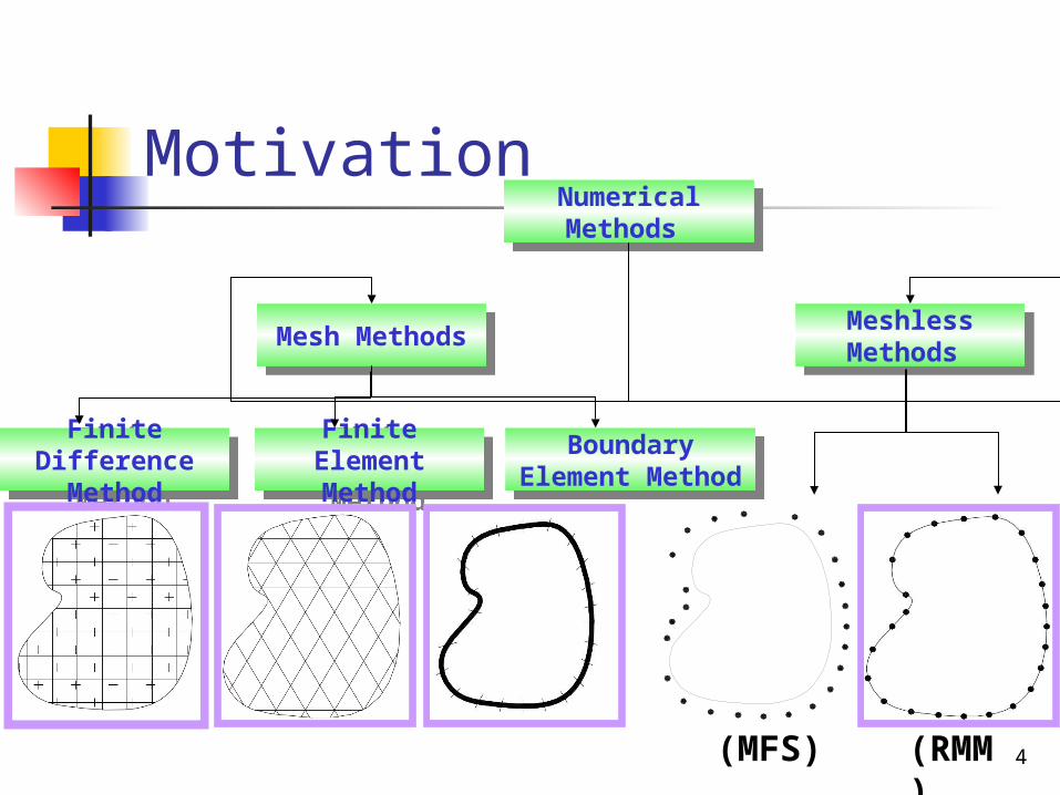
MotivationNumerical Methods Numerical Methods

Mesh MethodsMesh Methods

Finite Difference Method

Finite Difference Method

Meshless Methods Meshless Methods

Finite Element Method

Finite Element Method

Boundary Element Method

Boundary Element Method

(MFS) (RMM)

5

Outlines Motivation Statement of problem Method of fundamental solutions Desingularized meshless method Formulation for Cauchy problem Regularization techniques Numerical example Conclusions

6

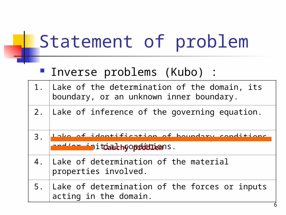
Statement of problem Inverse problems (Kubo) :

1. Lake of the determination of the domain, its boundary, or an unknown inner boundary.

2. Lake of inference of the governing equation.

3. Lake of identification of boundary conditions and/or initial conditions.

4. Lake of determination of the material properties involved.

5. Lake of determination of the forces or inputs acting in the domain.

Cauchy problem

7

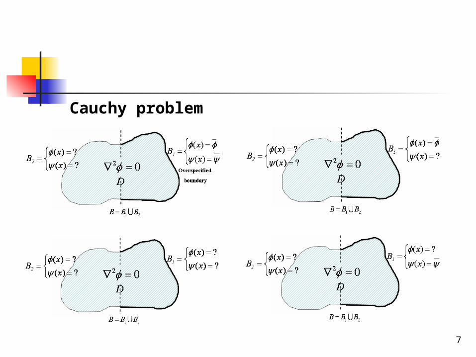
Cauchy problem

8

Outlines Motivation Statement of problem Method of fundamental solutions Desingularized meshless method Formulation for multiple holes Regularization techniques Numerical example Conclusions

9

Method of fundamental solutions (MFS)

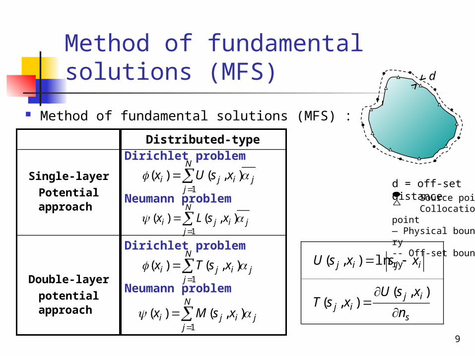
Method of fundamental solutions (MFS) :

Source point Collocation point— Physical boundary-- Off-set boundary

d = off-set distance

d

Double-layer

potential approach

Single-layer

Potential approach

Dirichlet problem

Neumann problem

Dirichlet problem

Neumann problem

Distributed-type

N

jjiji xsUx

1

),()(

N

jjiji xsLx

1

),()(

ijij xsxsU ln),(

s

ijij n

xsUxsT

),(),(

N

jjiji xsTx

1

),()(

N

jjiji xsMx

1

),()(

10

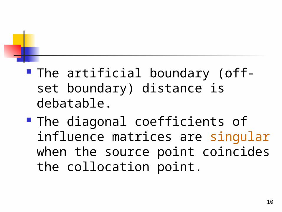
The artificial boundary (off-set boundary) distance is debatable.

The diagonal coefficients of influence matrices are singular when the source point coincides the collocation point.

11

Outlines Motivation Statement of problem Method of fundamental solutions Desingularized meshless method Formulation for Cauchy problem Regularization techniques Numerical example Conclusions

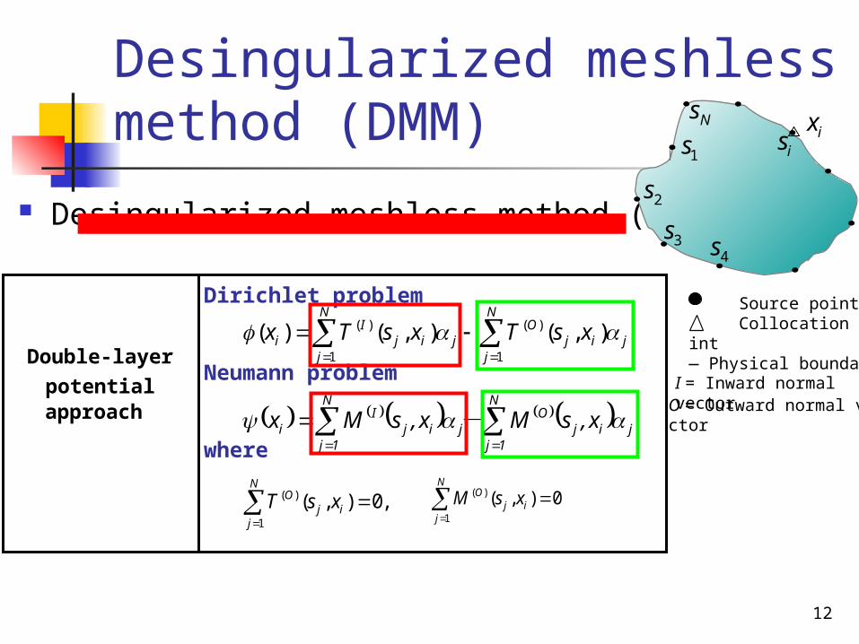
12

N

1jjij

ON

1jjij

Ii x,sMx,sMx －

Dirichlet problem

Neumann problem

where

N

jjij

ON

jjij

Ii xsTxsTx

1

)(

1

)( ),(),()(

Desingularized meshless method (DMM)

Source point Collocation point— Physical boundary

Desingularized meshless method (DMM)

Double-layer

potential approach

( )

1

( , ) 0,N

Oj i

j

T s x

( )

1

( , ) 0N

Oj i

j

M s x

ixis

1s

2s

3s4s

Ns

I = Inward normal vectorO = Outward normal vector

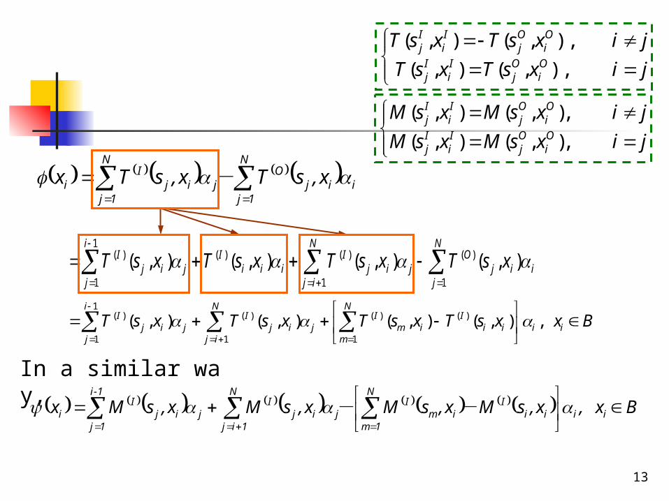
13

1( ) ( ) ( ) ( )

1 1 1

( , ) ( , ) ( , ) ( , ) ,i N N

I I I Ij i j j i j m i i i i i

j j i m

T s x T s x T s x T s x x B

N

1jiij

ON

1jjij

Ii x,sTx,sTx －

1( ) ( ) ( ) ( )

1 1 1

( , ) ( , ) ( , ) ( , )i N N

I I I Oj i j i i i j i j j i i

j j i j

T s x T s x T s x T s x

In a similar way,

jixsTxsT

jixsTxsTOi

Oj

Ii

Ij

Oi

Oj

Ii

Ij

),,(),(

),,(),(

( , ) ( , ),

( , ) ( , ),

I I O Oj i j iI I O Oj i j i

M s x M s x i j

M s x M s x i j

Bx,x,sMx,sMx,sMx,sMx ii

N

1mii

Iim

IN

1ijjij

I1-i

1jjij

Ii

－－

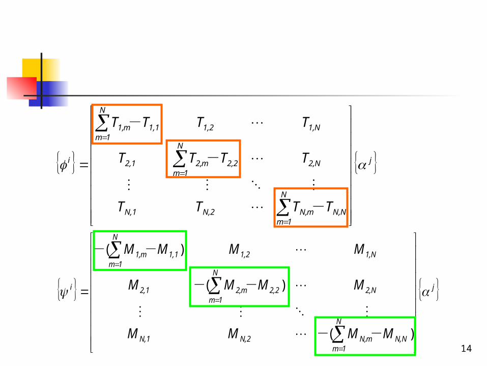
14

jN

1mNN,mN,N,2N,1

N2,

N

1m2,2m2,2,1

N1,1,2

N

1m1,1m1,

i

MMMM

MMMM

MMMM

)(

)(

)(

－－

－－

－－

j

N

1mNN,mN,N,2N,1

N2,

N

1m2,2m2,2,1

N1,1,2

N

1m1,1m1,

i

TTTT

TTTT

TTTT

－

－

－

15

Outlines Motivation Statement of problem Method of fundamental solutions Desingularized meshless method Formulation with Cauchy problem Regularization techniques Numerical example Conclusions

16

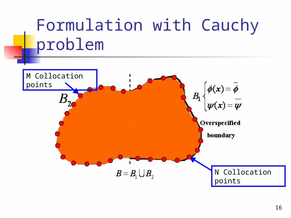
Formulation with Cauchy problem

N Collocation points

M Collocation points

17

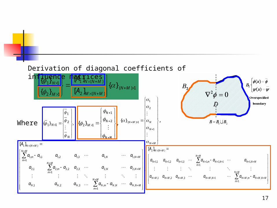
Derivation of diagonal coefficients of influence matrices.

1)()(2

)(1

12

11 }{][

][

}{

}{

MNMNM

MNN

M

N

A

A

Where ,

N

N

2

1

11}{ ,}{

MN

2N

1N

12

M

,

][

,1

,,3,2,1,

,2,23,21

2,2,21,2

,1,13,12,11

1,1,1

)(1

MNN

MN

mNNmNNNN

MNN

MN

mm

MNN

MN

mm

MNN

aaaaaa

aaaaaa

aaaaaa

A

MN

mMNMNmMNNMNMNMNMN

MNN

MN

mNNmNNNN

MNM

aaaaaa

aaaaaa

A

1,,1,3,2,1,

,11

1,1,13,12,11,1

)(2 ][

,}{

1

2

1

1)(

MN

N

NMN

18

1)()(2

)(1

12

11

][

][

}{

}{

MNMNM

MNN

M

N

B

B

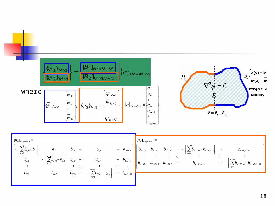
where

,

N

N

2

1

11}{ ,}{ 2

1

12

MN

N

N

M

,

1

2

1

1)(

MN

N

NMN

,

][

,1

,,3,2,1,

,2,23,21

2,2,21,2

,1,13,12,11

1,1,1

)(1

MNN

MN

mNNmNNNN

MNN

MN

mm

MNN

MN

mm

MNN

bbbbbb

bbbbbb

bbbbbb

B

MN

mMNMNmMNNMNMNMNMN

MNN

MN

mNNmNNNN

MNM

bbbbbb

bbbbbb

B

1,,1,3,2,1,

,11

1,1,13,12,11,1

)(2 ][

19

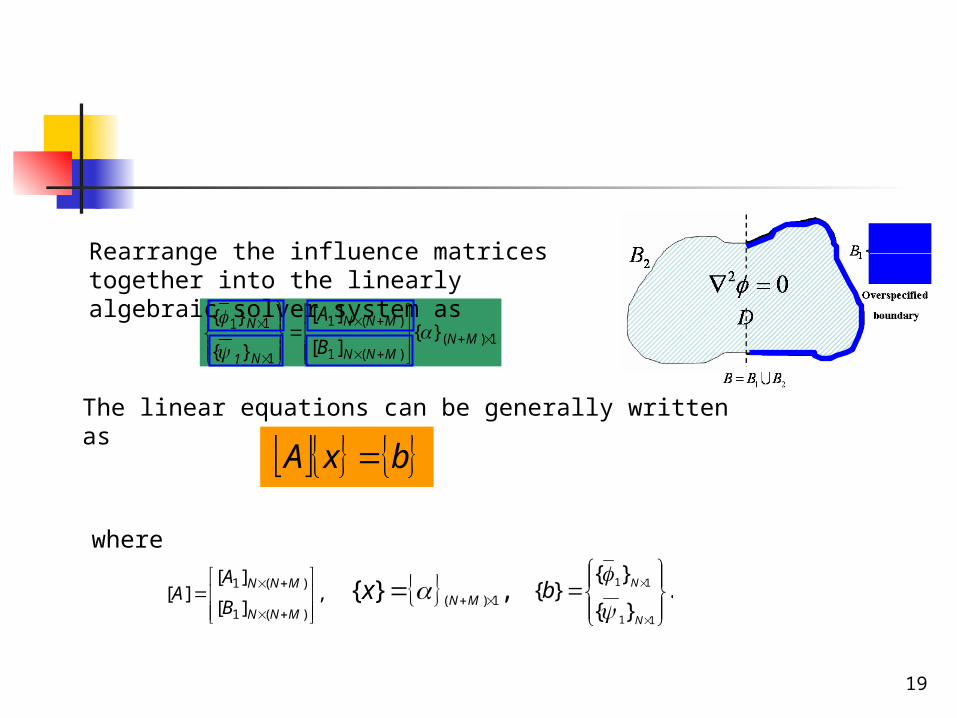
Rearrange the influence matrices together into the linearly algebraic solver system as

1)()(1

)(1

1

11 }{][

][

}{

}{

MNMNN

MNN

N1

N

B

A

The linear equations can be generally written as

bxA

where

,][

][][

)(1

)(1

MNN

MNN

B

AA ,}{ 1)( MNx .

}{

}{}{

11

11

N

Nb

20

Motivation Statement of problem Method of fundamental solutions Desingularized meshless method Formulation with Cauchy problem Regularization techniques Numerical example Conclusions

Outlines

21

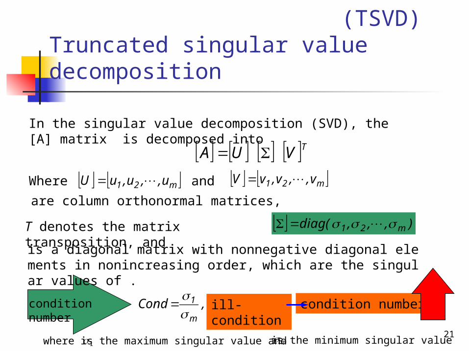
(TSVD)Truncated singular value decomposition

In the singular value decomposition (SVD), the [A] matrix is decomposed into

TVUA

Where m21 u,,u,uU m21 v,,v,v V and

are column orthonormal matrices,

T denotes the matrix transposition, and

),,,( diag m21

is a diagonal matrix with nonnegative diagonal elements in nonincreasing order, which are the singular values of .

condition number

, Condm

1

1 mwhere is the maximum singular value and is the minimum singular value

ill-condition condition number

22

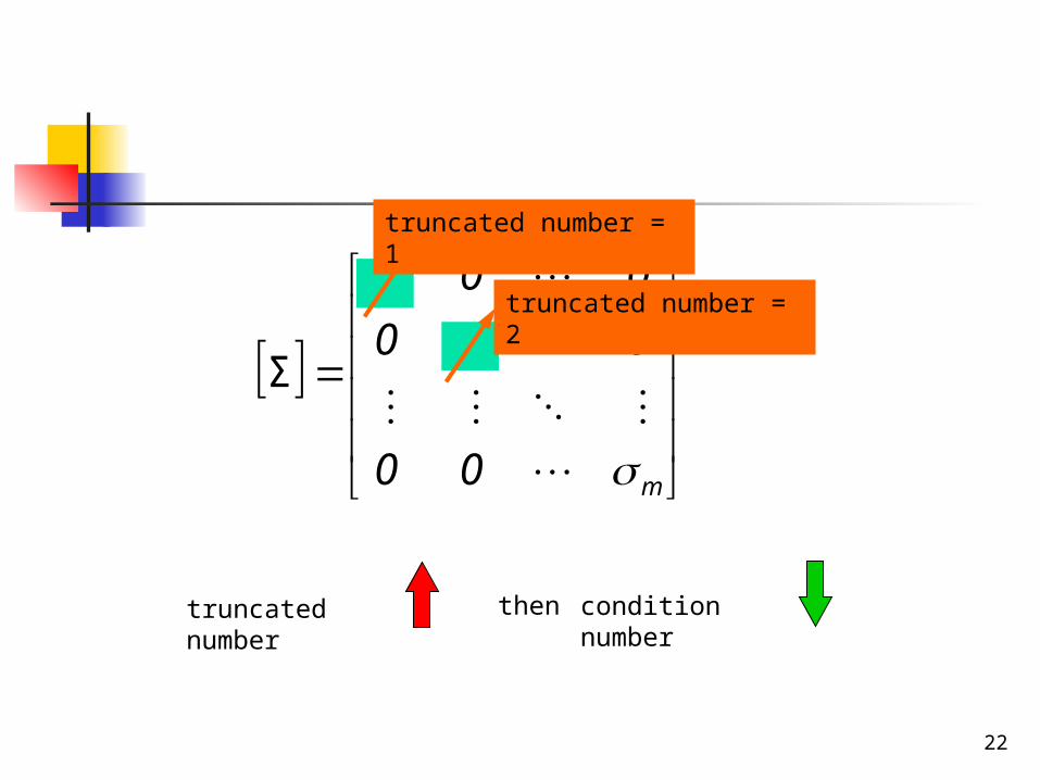
m

2

1

00

00

00

Σ

truncated number

then condition number

truncated number = 1

truncated number = 2

23

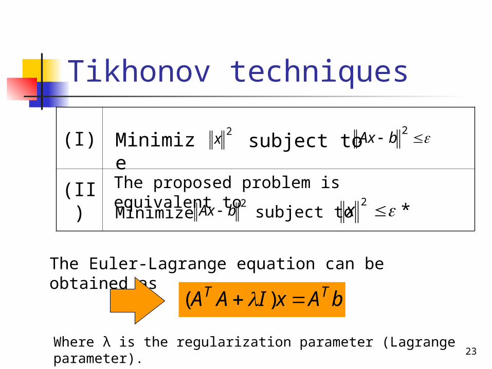
Tikhonov techniques

(I)

(II)

2x 2

bAxMinimize

subject to

The proposed problem is equivalent to Minimize

2bAx subject to *

2 x

The Euler-Lagrange equation can be obtained as

bAxIAA TT )(

Where λ is the regularization parameter (Lagrange parameter).

24

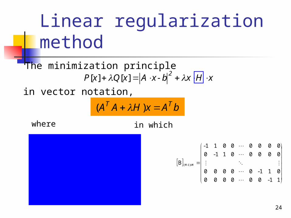
Linear regularization methodThe minimization principle

xHxb-xAxQxP2 ][][

in vector notation,

bAxHAA TT )( where

11-000000

1-21-00000

01-21-0000

00001-21-0

000001-21-

0000001-1

BBH M1)-(M1)-(MMT

MM

in which

11-000000

011-00000

0000011-0

00000011-

B M1)-(M

25

Outlines Motivation Statement of problem Method of fundamental solutions Desingularized meshless method Formulation for Cauchy problem Regularization techniques Numerical example Conclusions

26

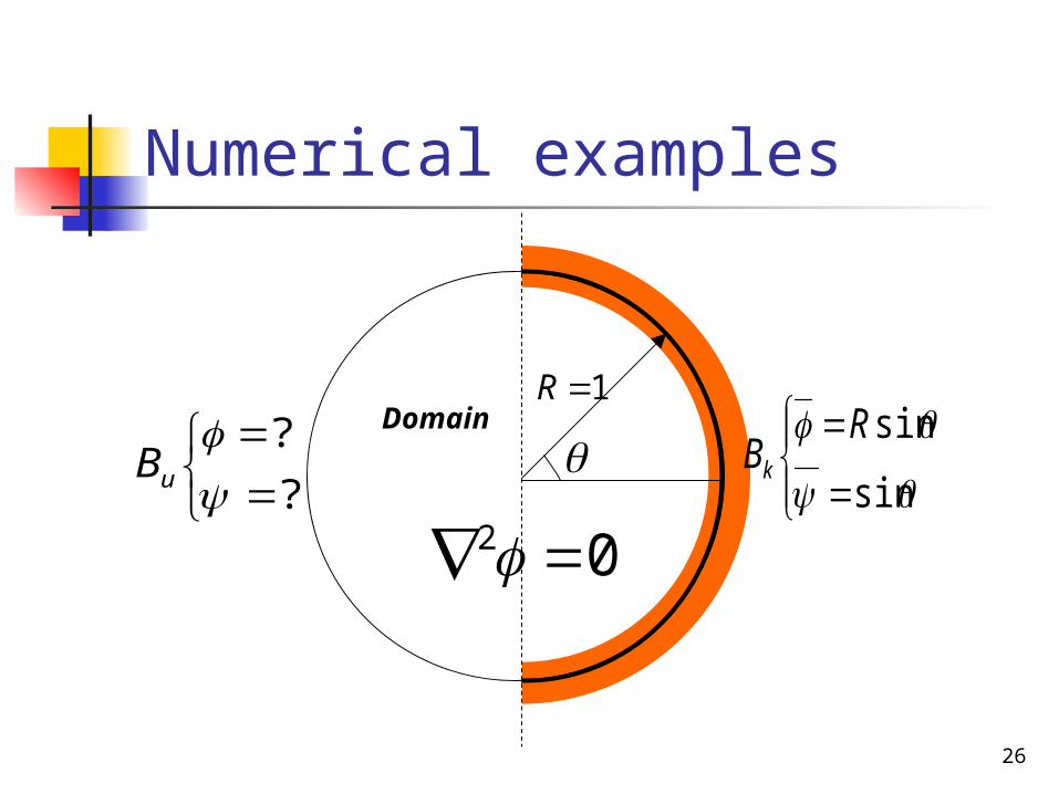
Numerical examples

1R

Domain

02

sin

sinRBk

?

?

uB

27

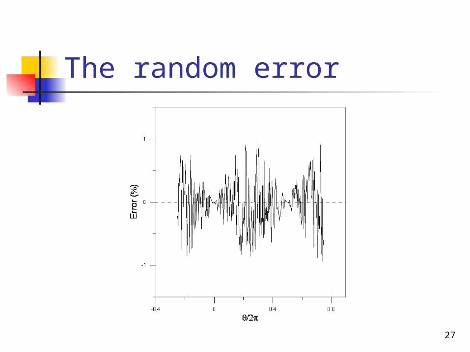
The random error

28

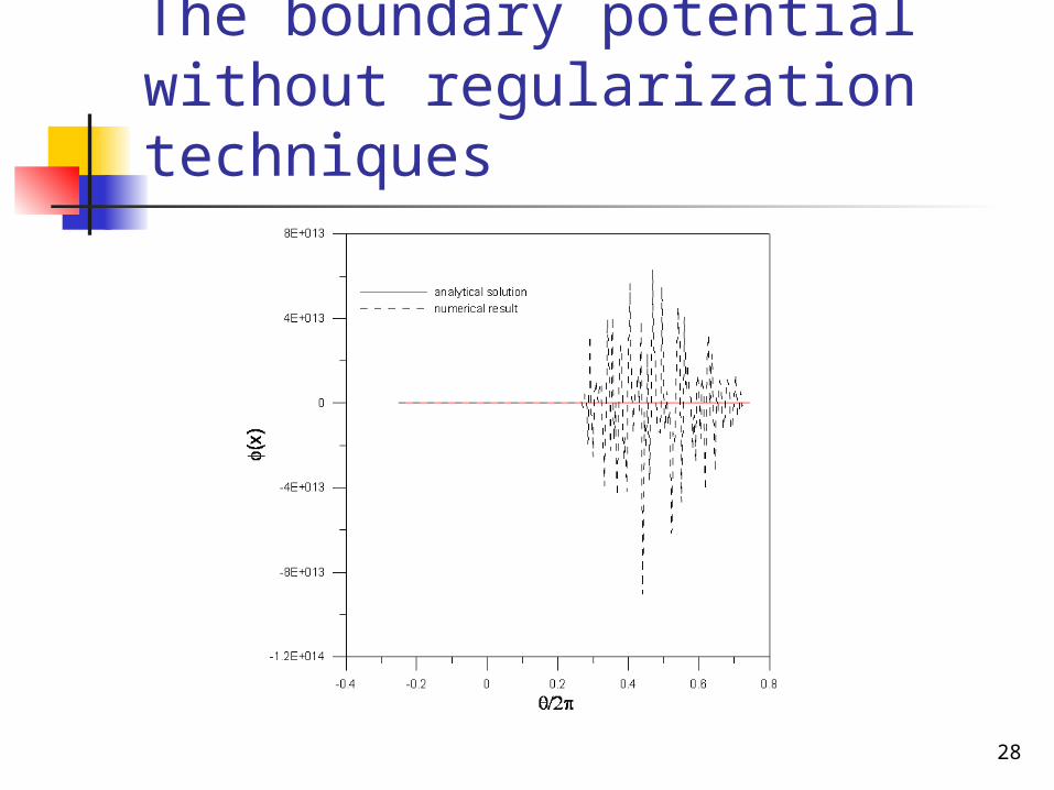
The boundary potential without regularization techniques

29

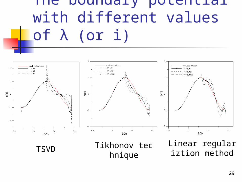
The boundary potential with different values of λ (or i)

TSVD Tikhonov technique

Linear regulariztion method

30

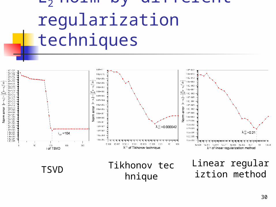
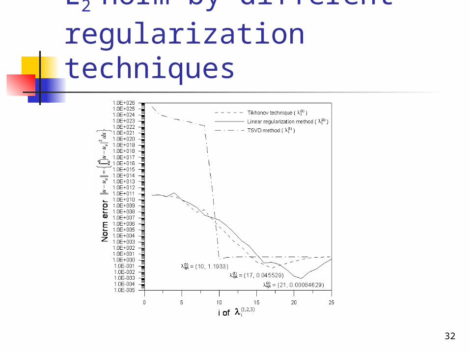
L2 norm by different regularization techniques

TSVD Tikhonov technique

Linear regulariztion method

31

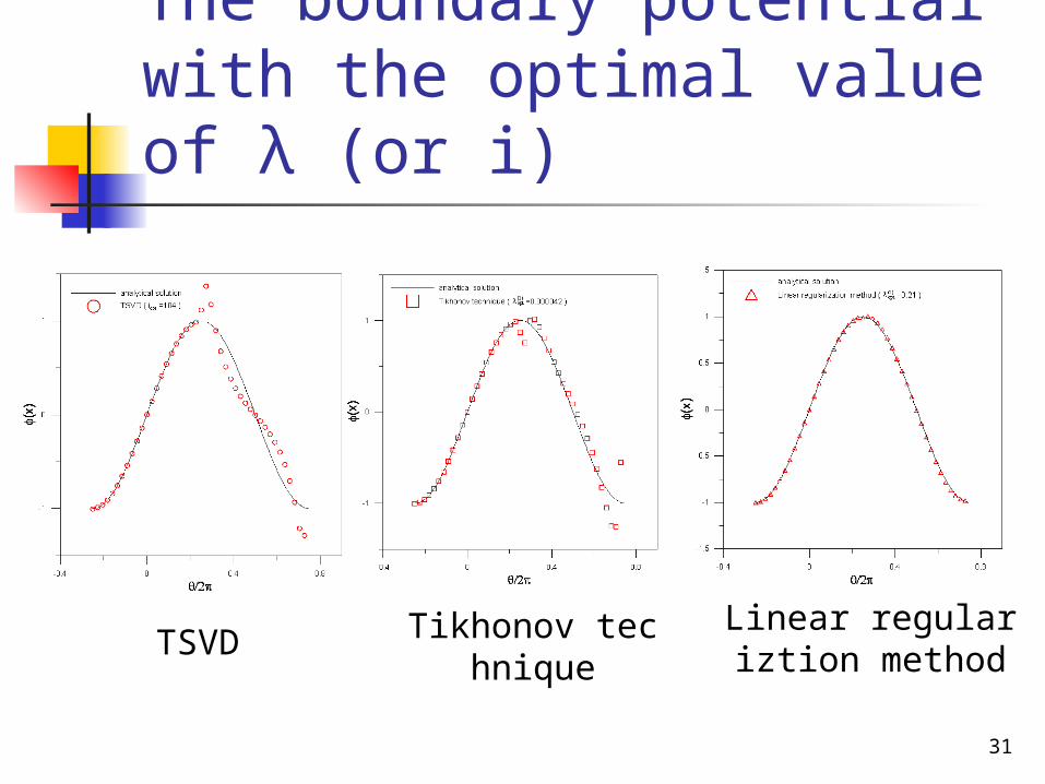
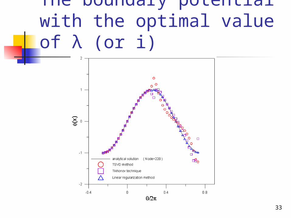
The boundary potential with the optimal value of λ (or i)

TSVD Tikhonov technique

Linear regulariztion method

32

L2 norm by different regularization techniques

33

The boundary potential with the optimal value of λ (or i)

34

Outlines Motivation Statement of problem Method of fundamental solutions Desingularized meshless method Formulation for Cauchy problem Regularization techniques Numerical examples Conclusions

35

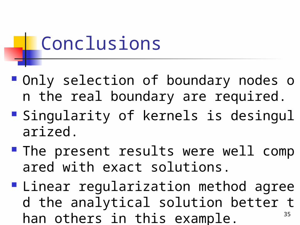
Conclusions

Only selection of boundary nodes on the real boundary are required.

Singularity of kernels is desingularized. The present results were well compared wit

h exact solutions. Linear regularization method agreed the an

alytical solution better than others in this example.

36

The end

Thanks for your attentions.

Your comment is much appreciated.