Embed Size (px)
Citation preview
Research Method
School of Economic Information EngineeringDr. Xu Yun ( 徐赟 )Office :Phone : Email : [email protected]
04/18/23 2
“Factor Analysis” A statistical technique used to
(1) estimate factors or latent variables (2) reduce the dimensionality of a large
number of variables to a fewer number of factors.
History: Idea first introduced by Karl Pearson (1901) First applied by Charles Spearman to study
human abilities (“general intelligence”) Thurstone (1931) developed “common-factor
theory”
04/18/23 3
Suppose we have some survey item-indicators of “job satisfaction”
Item 1: I am satisfied with my pay.
Item 2: I get along well with my peers at work.
Item 3: I am happy with my boss at work.
As part of scale development or evaluation: is my scales/measure unidimensional?
04/18/23 4
Variance of an Item or Indicator Factor analysis assumes that a variable's
variance is composed of three components: Common variance
variance in a variable shared with common factors Specific variance
component of unique variance which is reliable but not explained by common factors
Error variance unreliable and inexplicable variation in a variable
04/18/23 5
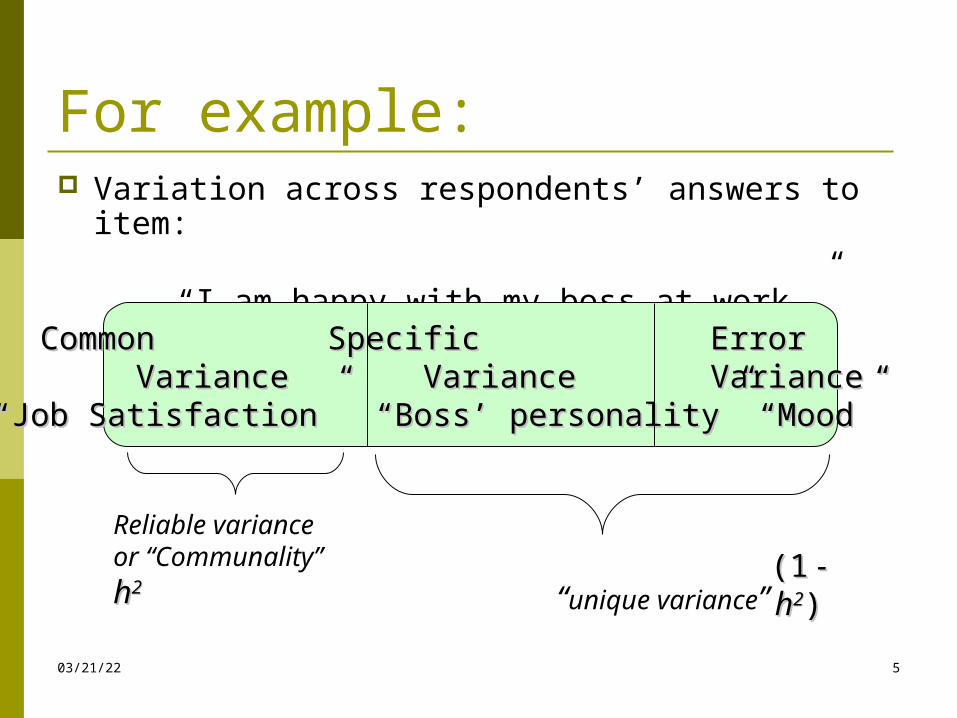
For example: Variation across respondents’ answers to item:
“I am happy with my boss at work.”
“unique variance”
Common Common SpecificSpecific ErrorErrorVarianceVariance VarianceVariance VarianceVariance““Job Satisfaction”Job Satisfaction” “Boss’ personality”“Boss’ personality” “Mood”“Mood”
Reliable variance or
“Communality” hh22 (1(1 - h - h22))
04/18/23 6
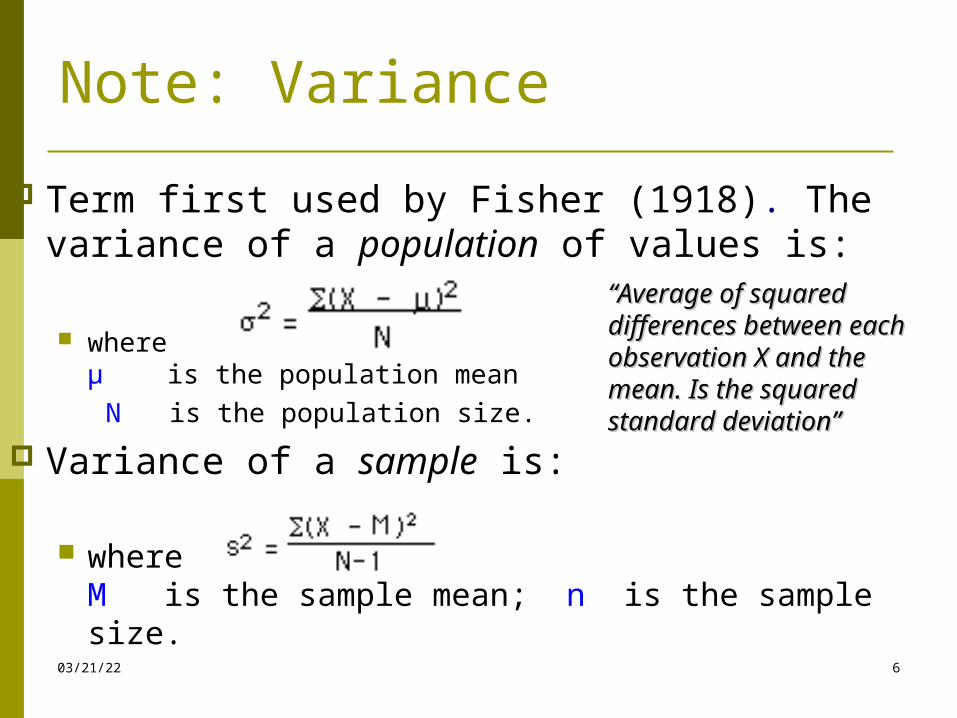
Note: Variance
Term first used by Fisher (1918). The variance of a population of values is:
where
µ is the population mean N is the population size.
Variance of a sample is:
whereM is the sample mean; n is the sample size.
““Average of squared Average of squared differences between each differences between each observation X and the observation X and the mean. Is the squared mean. Is the squared standard deviation”standard deviation”
04/18/23 7
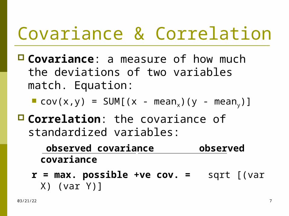
Covariance & Correlation Covariance: a measure of how much the
deviations of two variables match. Equation: cov(x,y) = SUM[(x - meanx)(y - meany)]
Correlation: the covariance of standardized variables:
observed covariance observed covariance
r = max. possible +ve cov. = sqrt [(var X) (var Y)]
04/18/23 8
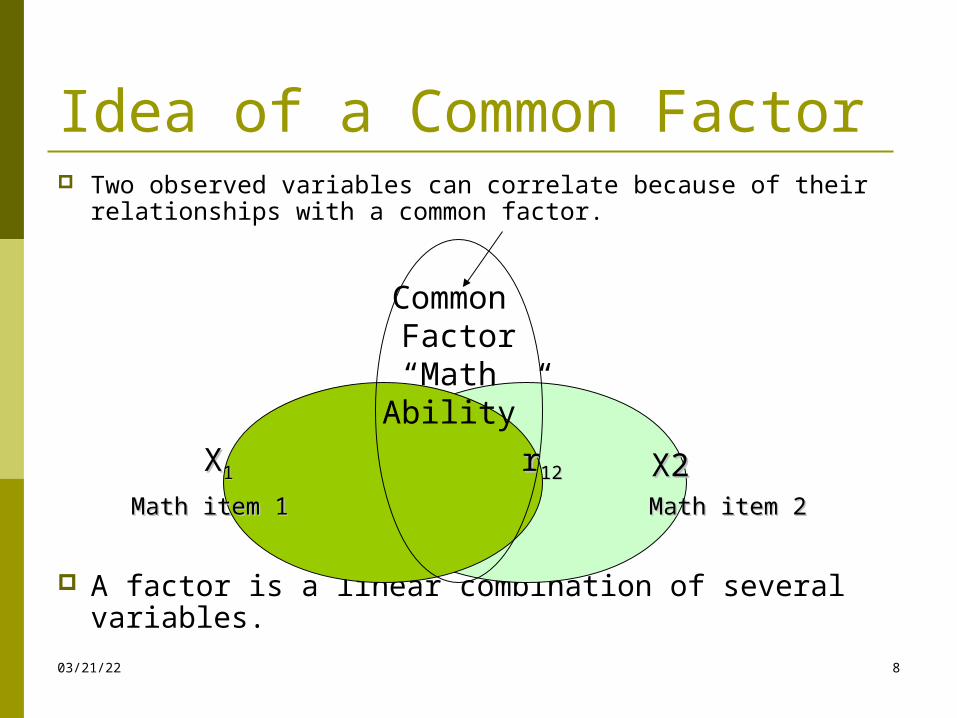
Idea of a Common Factor Two observed variables can correlate because of their
relationships with a common factor.
A factor is a linear combination of several variables.
X2X2 Math item 2Math item 2
XX11 r r1212
Math item 1Math item 1
Common Factor“Math Ability”
04/18/23 9
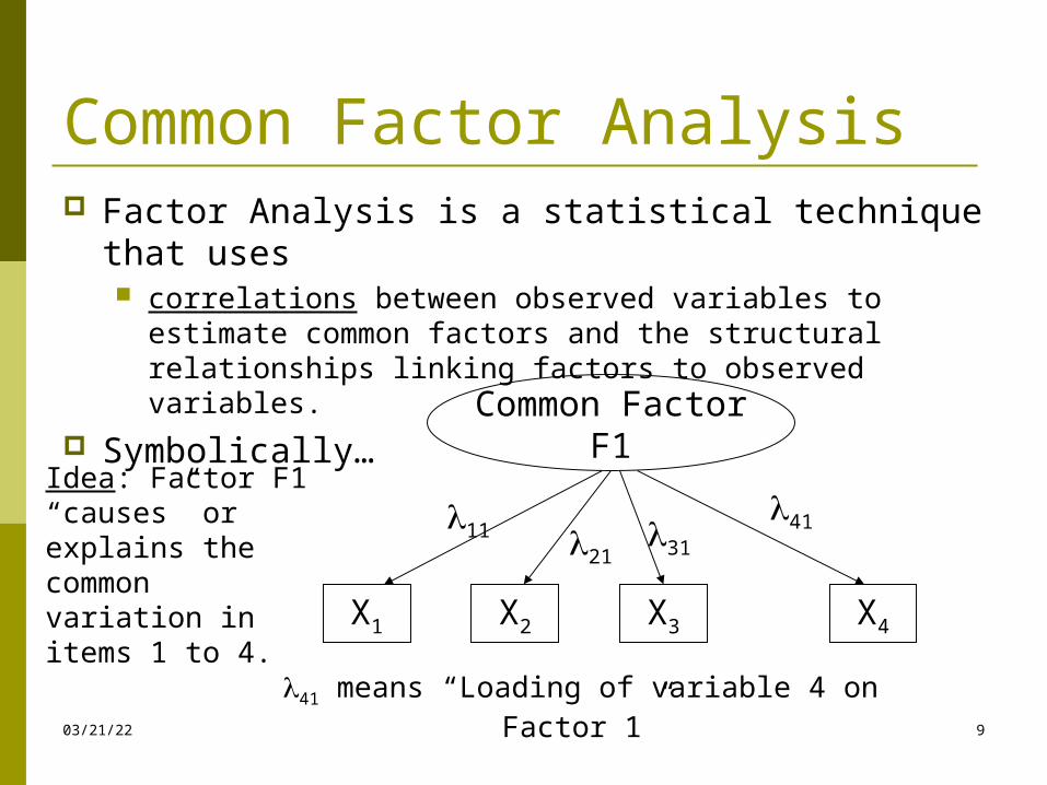
Common Factor Analysis Factor Analysis is a statistical technique that uses
correlations between observed variables to estimate common factors and the structural relationships linking factors to observed variables.
Symbolically…Common Factor
F1
X1 X2 X3 X4
413121
11
41 means “Loading of variable 4 on Factor 1”
Idea: Factor F1 “causes” or explains the common variation in items 1 to 4.
04/18/23 10
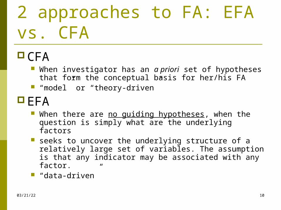
2 approaches to FA: EFA vs. CFA CFA
When investigator has an a priori set of hypotheses that form the conceptual basis for her/his FA
“model” or “theory-driven”
EFA When there are no guiding hypotheses, when the
question is simply what are the underlying factors seeks to uncover the underlying structure of a relatively
large set of variables. The assumption is that any indicator may be associated with any factor.
“data-driven”
04/18/23 11
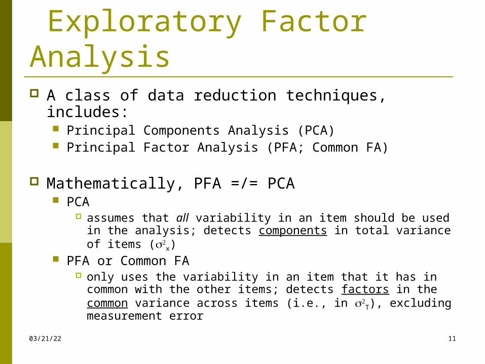
Exploratory Factor Analysis A class of data reduction techniques, includes:
Principal Components Analysis (PCA) Principal Factor Analysis (PFA; Common FA)
Mathematically, PFA =/= PCA PCA
assumes that all variability in an item should be used in the analysis; detects components in total variance of items (
x) PFA or Common FA
only uses the variability in an item that it has in common with the other items; detects factors in the common variance across items (i.e., in
T), excluding measurement error
04/18/23 12
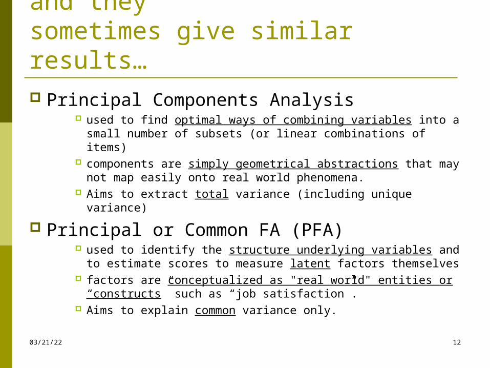
Although steps are similar and they sometimes give similar results…
Principal Components Analysis used to find optimal ways of combining variables into a
small number of subsets (or linear combinations of items) components are simply geometrical abstractions that may
not map easily onto real world phenomena. Aims to extract total variance (including unique variance)
Principal or Common FA (PFA) used to identify the structure underlying variables and to
estimate scores to measure latent factors themselves factors are conceptualized as "real world" entities or
“constructs” such as “job satisfaction”. Aims to explain common variance only.
04/18/23 13
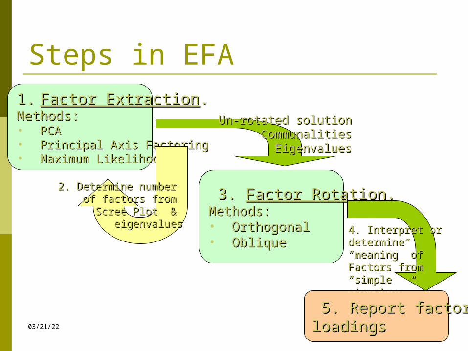
Steps in EFA1.1. Factor ExtractionFactor Extraction..Methods:Methods:• PCAPCA• Principal Axis FactoringPrincipal Axis Factoring• Maximum LikelihoodMaximum Likelihood
3. 3. Factor RotationFactor Rotation..Methods:Methods:• OrthogonalOrthogonal• ObliqueOblique
Un-rotated solutionUn-rotated solutionCommunalitiesCommunalities
EigenvaluesEigenvalues
2. Determine number 2. Determine number of factors from of factors from
Scree Plot & Scree Plot & eigenvalueseigenvalues
4. Interpret or 4. Interpret or determine “meaning” determine “meaning” of Factors from of Factors from “simple structure”“simple structure”
5. Report factor 5. Report factor loadingsloadings
04/18/23 14
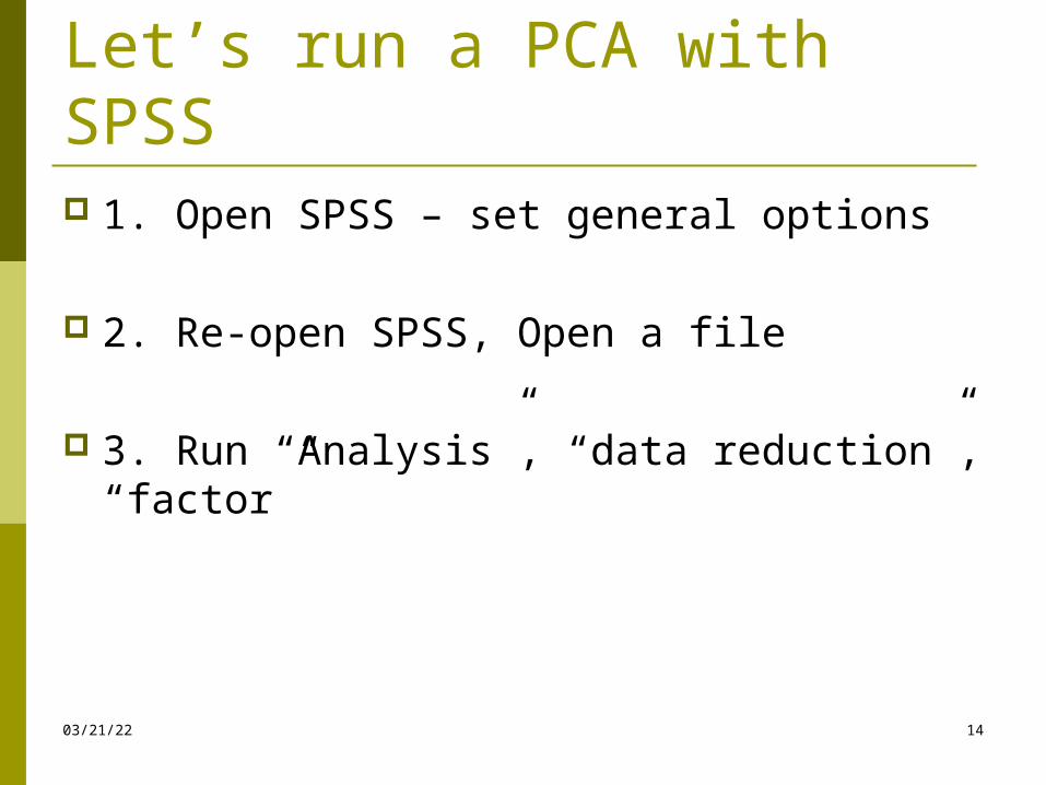
Let’s run a PCA with SPSS 1. Open SPSS – set general options
2. Re-open SPSS, Open a file
3. Run “Analysis”, “data reduction”, “factor”
04/18/23 15
Limitation of EFA EFA was designed to fit the data
will find you some “factors” whether you expected these factors or not…
interpretation of factors measured by a few variables can be quite complicated because the researcher lacks prior knowledge
and therefore has no basis on which to make an interpretation.
Mulaik (1972): EFA at best suggests hypotheses for further research; does not justify knowledge.
04/18/23 16
Confirmatory Factor Analysis Seeks to determine if the number of factors and
the loadings of measured (indicator) variables on them conform to what is expected on the basis of pre-established theory.
A priori assumption is that each factor (the number and labels of which may be specified à priori) is associated with a specified subset of indicator variables.
Minimum requirement for CFA: hypothesize beforehand the number of factors in the model also expectations about which variables will
load on which factors (Kim and Mueller, 1978b: 55).
04/18/23 17
Confirmatory factor analysis A theory-testing model as opposed to a
theory-generating method like EFA: researcher begins with a hypothesis prior to
the analysis. The model or hypothesis specifies
which variables will be correlated with which factors which factors are correlated.
The hypothesis should be based on a strong theoretical and/or empirical foundation (Stevens, 1996).
04/18/23 18
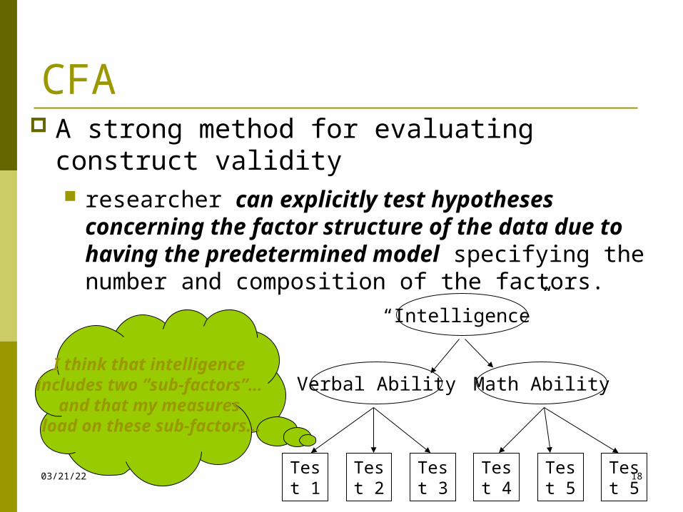
CFA A strong method for evaluating construct
validity researcher can explicitly test hypotheses
concerning the factor structure of the data due to having the predetermined model specifying the number and composition of the factors.
Test 1
Verbal Ability Math Ability
“Intelligence”
Test 2
Test 3
Test 4
Test 5
Test 5
I think that intelligence includes two “sub-factors”…
and that my measures load on these sub-factors...
04/18/23 19
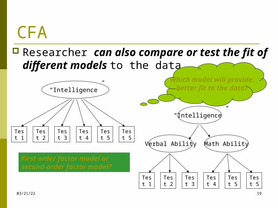
CFA Researcher can also compare or test the
fit of different models to the data
Test 1
“Intelligence”
Test 2
Test 3
Test 4
Test 5
Test 5
Test 1
Verbal Ability Math Ability
“Intelligence”
Test 2
Test 3
Test 4
Test 5
Test 5
Which model will provide better fit to the data?
First order factor model or second-order factor model?
04/18/23 20
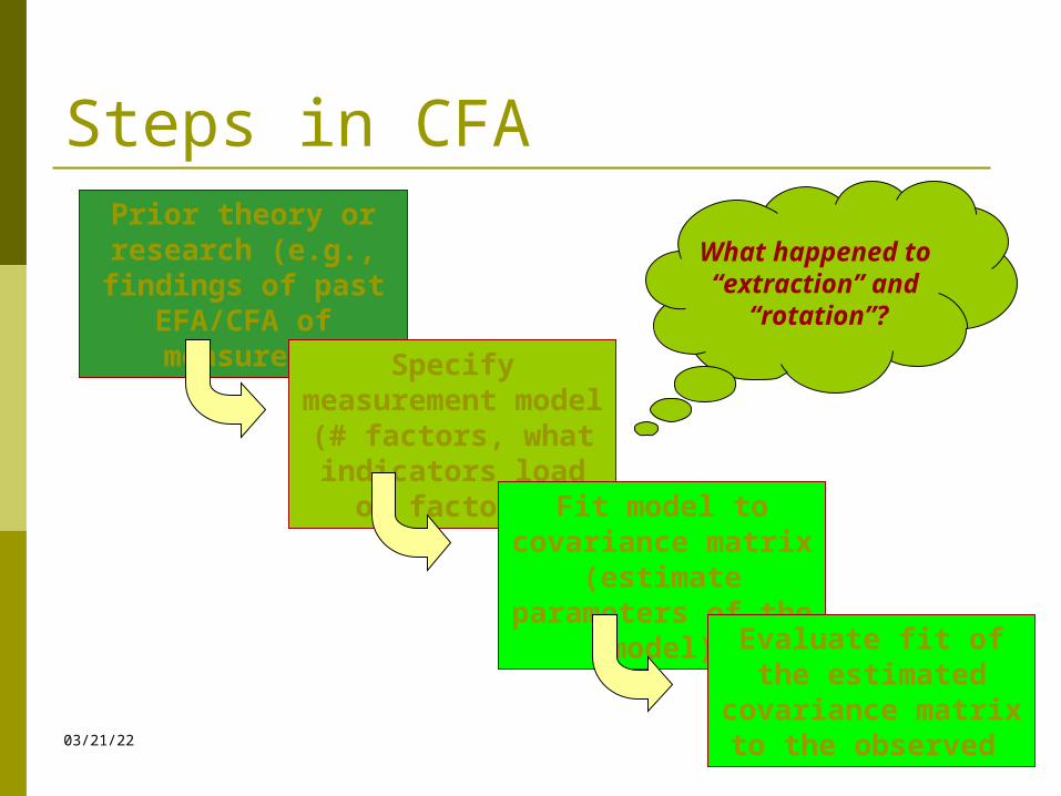
Steps in CFAPrior theory or research
(e.g., findings of past EFA/CFA of measure)
Specify measurement model (# factors, what
indicators load on factors)
Fit model to covariance matrix (estimate
parameters of the model)
Evaluate fit of the estimated covariance
matrix to the observed
What happened to “extraction” and
“rotation”?
04/18/23 21
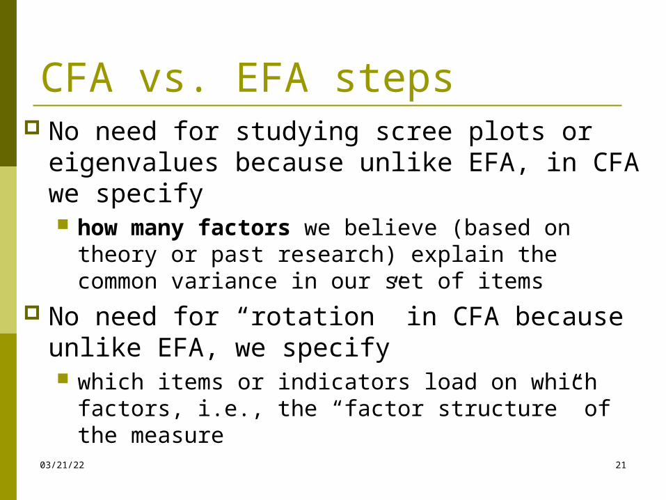
CFA vs. EFA steps No need for studying scree plots or
eigenvalues because unlike EFA, in CFA we specify how many factors we believe (based on theory
or past research) explain the common variance in our set of items
No need for “rotation” in CFA because unlike EFA, we specify which items or indicators load on which factors,
i.e., the “factor structure” of the measure
04/18/23 22
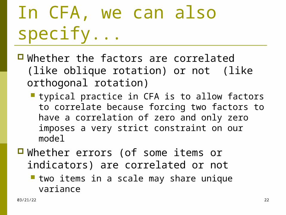
In CFA, we can also specify... Whether the factors are correlated (like
oblique rotation) or not (like orthogonal rotation) typical practice in CFA is to allow factors to
correlate because forcing two factors to have a correlation of zero and only zero imposes a very strict constraint on our model
Whether errors (of some items or indicators) are correlated or not two items in a scale may share unique
variance
04/18/23 23
To perform a CFA... You must know…
The LISREL framework or language for Structural Equation Modeling
Path diagrams LISREL syntax programming How to read a LISREL output
04/18/23 24
Method of Extraction #1:
Principal Components Analysis PCA seeks
a linear combination of variables such that maximum variance is extracted from the variables then removes this variance and seeks a second linear
combination which explains the maximum proportion of the remaining variance, and so on.
a set of factors that account for all the common and unique variance in a set of variables
applies it to a correlation matrix in which the diagonal elements are 1's
04/18/23 25
Principal Components Analysis The extraction of principal components
amounts to a variance maximizing (varimax) rotation of the original variable space.
For example, in a scatterplot we can think of the regression line as the original X axis, rotated so that it approximates the regression line.
In variance maximizing, the goal of the rotation is to maximize the variance variability of the "new" variable (factor), while minimizing the variance around the new variable.
04/18/23 26
PFA Method of Extraction #2
Principal Axis Factoring (PFA) Seeks the least number of factors that can
account for the common variance of a set of variables (minus unique variances or errors)
Applies to a correlation matrix in which the diagonal elements are not 1's, but estimates of the communalities are usually the squared multiple correlations of
each variable with the remainder of variables in the matrix
04/18/23 27
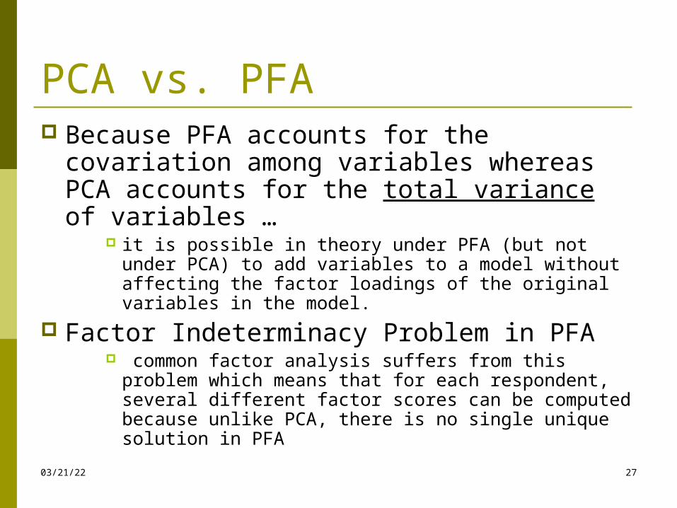
PCA vs. PFA Because PFA accounts for the covariation
among variables whereas PCA accounts for the total variance of variables …
it is possible in theory under PFA (but not under PCA) to add variables to a model without affecting the factor loadings of the original variables in the model.
Factor Indeterminacy Problem in PFA common factor analysis suffers from this problem
which means that for each respondent, several different factor scores can be computed because unlike PCA, there is no single unique solution in PFA
04/18/23 28
Important terms in EFA Communality (of an item or variable)
Eigenvalue (of a factor)
Factor loading (of an item to a factor)
Factor score
04/18/23 29
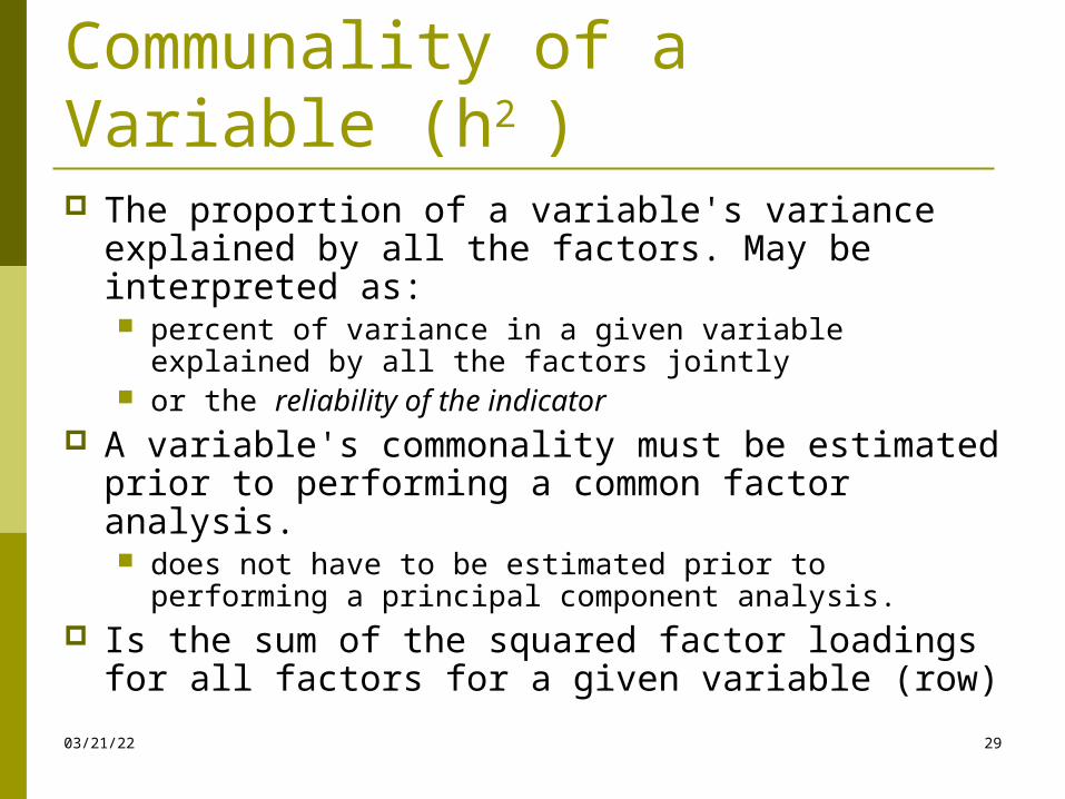
Communality of a Variable (h2 ) The proportion of a variable's variance explained
by all the factors. May be interpreted as: percent of variance in a given variable explained by all
the factors jointly or the reliability of the indicator
A variable's commonality must be estimated prior to performing a common factor analysis. does not have to be estimated prior to performing a
principal component analysis. Is the sum of the squared factor loadings for all
factors for a given variable (row)
04/18/23 30
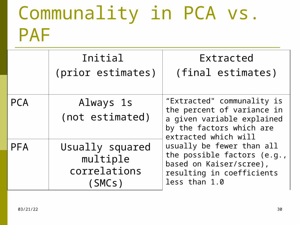
Communality in PCA vs. PAF
Initial (prior estimates)
Extracted(final estimates)
PCA Always 1s(not estimated)
“Extracted" communality is the percent of variance in a given variable explained by the factors which are extracted which will usually be fewer than all the possible factors (e.g., based on Kaiser/scree), resulting in coefficients less than 1.0
PFA Usually squared multiple correlations
(SMCs)
04/18/23 31
Communality Estimates for PFA Prior communality estimates are estimated prior to
the factor analysis. Common methods are to use: (1) an independent reliability estimate (2) the squared multiple correlation between each
variable and the other variables (3) the highest off-diagonal correlation for each variable, (4) iterate by performing a sequence of factor analyses
using the final communality estimates from one analysis as prior communality estimates for the next analysis.
Final communality estimates are the sum of squared loadings for a variable in an orthogonal factor matrix.
04/18/23 32
Interpreting Communality Communalities must be interpreted in relation to
the interpretability of the factors. A communality of .75 seems high but is meaningless
unless the factor on which the variable is loaded is interpretable, which it usually will be.
A communality of .25 seems low but may be meaningful if the item is contributing to a well-defined factor.
What is critical is not the communality coefficient per se, but rather the extent to which the item plays a role in the interpretation of the factor, though often this role is greater when communality is high.
04/18/23 33
Eigenvalue of a Factor Definition
The eigenvalue for a given factor reflects the variance in all the variables accounted for by that factor.
If a factor has a low eigenvalue, it is contributing little to the explanation of variances in the variables and may be ignored as redundant with more important factors.
Computation A factor's eigenvalue may be computed as the sum of its
squared factor loadings for all the variables. Note that the eigenvalues associated with the unrotated
and rotated solution will differ, though their total will be the same.
04/18/23 34
Important points -- Eigenvalues Refer to variances extracted by the
factors.
Sum of the eigenvalues is equal to the number of variables
Used to indicate the “percent of the total or common variance” accounted for by a factor.
04/18/23 35
How many Factors to Extract? As we extract consecutive factors, they
account for less and less variability. The decision of when to stop extracting
factors basically depends on when there is only very little "random" variability left.
The nature of this decision is arbitrary; but various guidelines have been developed: Kaiser criterion Scree test
04/18/23 36
Kaiser criterion Proposed by Kaiser (1960)
Retain only factors with eigenvalues >1 Idea
Unless a factor extracts at least as much as the equivalent of one original variable, we drop it.
Note: Kaiser criterion sometimes retains too many
factors

04/18/23 37
Scree test First proposed by Cattell (1966):
plot the eigenvalues in a simple line plot find the place where the smooth decrease of
eigenvalues appears to the right of the plot Note:
"scree" is a geological term referring to the debris which collects on the lower part of a rocky slope.
scree test sometimes retains too few factors both Kaiser & scree tests do quite well under normal
conditions, that is, when there are relatively few factors and many cases
04/18/23 38
Other Considerations Variance explained criteria:
Some researchers simply use the rule of keeping enough factors to account for 90% (sometimes 80%) of the variation.
Joliffe criterion: Less used, more liberal rule of thumb that may result in
twice as many factors as the Kaiser criterion. The Joliffe rule is to crop all components with eigenvalues under .7.
Comprehensibility. Though not a strictly mathematical criterion, there is
much to be said for limiting the number of factors to those whose dimension of meaning is readily comprehensible. Often this is the first two or three.
04/18/23 39
Rotation The step in factor analysis that allows you
to identify meaningful factor names or descriptions like these.
Goal: To obtain a clear pattern of loadings
sometimes referred to as simple structure where factors that are marked by high loadings for some variables and low loadings for others.
To make the output more understandable and is usually necessary to facilitate the interpretation of factors.
04/18/23 40
“Simple Structure” Louis Thurstone's interpretability criteria for
factor structures. A factor matrix for k factors exhibits simple structure if: Each variable has at least one zero loading. Each factor in a factor matrix with k columns should
have k zero loadings. Each pair of columns in a factor matrix should have
several variables loading on one factor but not the other. Each pair of columns should have a large proportion of
variables with zero loadings in both columns. Each pair of columns should only have a small
proportion of variable with non zero loadings in both columns.
04/18/23 41
Methods of Rotation Orthogonal vs. oblique
Orthogonal rotation requires factors to remain uncorrelated; others are oblique rotations.
a simple rule is that if there is any ability to print out a matrix of factor correlations, then the rotation is oblique.
Oblique rotations often achieve greater simple structure, though at a cost:
tend to produce correlated factors with many cross-loadings are often not easily interpreted.
04/18/23 42
Methods of Rotation in SPSS No rotation
The original, unrotated principal components solution maximizes the sum of squared factor loadings, efficiently creating a set of factors which explain as much of the variance in the original variables as possible.
Hard to interpret because variables tend to load on multiple factors.
Varimax rotation Orthogonal rotation of the factor axes to maximize the variance of the
squared loadings of a factor (column) on all the variables (rows) in a factor matrix
Has the effect of differentiating the original variables by extracted factor. That is, it minimizes the number of variables which have high loadings on any one given factor. Each factor will tend to have either large or small loadings of particular variables on it.
Yields results that make it as easy as possible to identify each variable with a single factor. This is the most common rotation option.
04/18/23 43
Method of Rotation in SPSS Quartimax (Orthogonal)
an orthogonal alternative which minimizes the number of factors needed to explain each variable.
Equimax (Orthogonal) a compromise between Varimax and Quartimax criteria.
Direct oblimin (Oblique) the standard method when one wishes a non-orthogonal
solution -- that is, one in which the factors are allowed to be correlated. Results in higher eigenvalues but diminished interpretability of the factors.
Promax (oblique) an alternative non-orthogonal rotation method which is
computationally faster than the direct oblimin method and therefore is sometimes used for very large datasets.
04/18/23 44
Communalities & Eigenvaluesafter Rotation
Communality does not change when rotation is carried out hence in SPSS there is only one communalities
table.
Eigenvalues of particular factors change after rotation … but the sum of eigenvalues is not affected by
rotation.
04/18/23 45
Factor loadings Called component loadings in PCA Refer to correlation coefficients between
the variables (rows) and factors (columns). Like with Pearson's r, the squared factor
loading is the percent of variance in that variable explained by the factor. A .30 loading means that the factor accounts
for about 10% of the variance in that variable A loading must exceed .70 for the factor to
explain 50% of the variance in that variable
04/18/23 46
Magnitude of Factor Loadings How high does a factor loading have to be to
consider that variable as a defining part of that factor? This is purely arbitrary, but common social science
practice uses a minimum cut-off of .3 or .35. Another arbitrary rule-of-thumb terms loadings as
"weak" if less than .4 "strong" if more than .6, and otherwise as
"moderate." Bottom-line: The meaning of the factor loading
magnitudes varies by research context. For instance, loadings of .45 might be considered
"high" for dichotomous items but for Likert scales a .6 might be required to be considered "high."
04/18/23 47
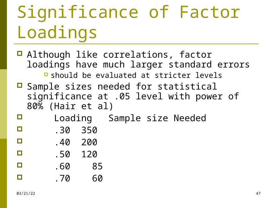
Significance of Factor Loadings Although like correlations, factor loadings have
much larger standard errors should be evaluated at stricter levels
Sample sizes needed for statistical significance at .05 level with power of 80% (Hair et al)
Loading Sample size Needed .30 350 .40 200 .50 120 .60 85 .70 60
04/18/23 48
Significance of Factor Loadings Small factor loadings can be significant when:
sample size is large a large number of variables is analysed the lesser the number of factors
04/18/23 49
Two Matrices produced by Oblique Rotation
Factor pattern matrix analogous to standardised regression coefficients each element indicates the importance of that
variable to the factor given other variables
Factor structure matrix elements are simple correlations of the variables with
the factors They are factor loadings
Note: Both matrices are identical with orthogonal rotation
04/18/23 50
Pattern vs. Structure matrix Most researchers report factor
pattern matrix because as the correlation correlation between
factors becomes greater, it becomes more difficult to distinguish which variables load uniquely on which factor
because “loadings” in factor structure matrix contain both the unique variance between variables and factors, and the correlation among the factors
04/18/23 51
EFA & Scale/Item analysis What variables should we consider deleting
after performing an EFA? Loadings:
Variables with several high loadings on different factors are not telling us anything unique
Variables that load on the unexpected factor(s) Communalities: Variables with very low
communalities below .25
04/18/23 52
Factor analysis and Validity In confirmatory factor analysis (CFA), a
finding that indicators have high loadings on the predicted factors indicates convergent validity.
In an oblique rotation, discriminant validity is demonstrated if the correlation between factors is not so high (ex., > .85) as to lead one to think the two factors overlap conceptually.
04/18/23 53
Factor Scores Description
Also called component scores in PCA, factor scores are the scores of each case (row) on each factor (column).
Computation To compute the factor score for a given case
for a given factor, one takes the case's standardized score on each variable, multiplies by the corresponding factor loading of the variable for the given factor, and sums these products.
04/18/23 54
Factor Scores The SPSS FACTOR procedure saves standardized
factor scores as variables in your working data file. By default it will name them FAC1_1,FAC2_1, FAC3_1,
etc., for the corresponding factors (factor 1, 2 and 3) of analysis 1; and FAC1_2, FAC2_2, FAC3_2 for a second set of factor scores, if any, within the same procedure, and so on. Although
SPSS adds these variables to the right of your working data set automatically, they will be lost when you close the dataset unless you re-save your data.
04/18/23 55
“Products” of FA for data reduction Select Surrogate measures
select the variable with the highest loading to represent that factor
Create summated (Likert) scales by using the sum or average response to a set of
variables, we reduce the measurement error relative to true score
Compute factor scores unlike summated scale scores, factor scores give
more weight to variables with higher loadings not preferred due to factor indeterminacy problem
04/18/23 56
What Sample size for EFA? No scientific answer, and methodologists differ.
New view is emerging (to challenge old view) Old view: Arbitrary Subject-to-Variables (STV) "rules of
thumb," in descending order of popularity, include:1. Rule of 10. There should be at least 10 cases for each item in
the instrument being used. 2. STV ratio. The subjects-to-variables (STV) ratio should be no
lower than 5 (Bryant and Yarnold, 1995) 3. Rule of 100: The number of subjects should be the larger of 5
times the number of variables, or 100. Even more subjects are needed when communalities are low and/or few variables load on each factor. (Hatcher, 1994)
4. Rule of 200. There should be at least 200 cases, regardless of STV (Gorsuch, 1983)
From Garson
04/18/23 57
“New” (non-STV ratio) view The clearer the true factor structure, the smaller
the sample size needed to discover it. But it would be very difficult to discover even a very
clear and simple factor structure with fewer than about 50 cases, and 100 or more cases would be much preferable for a less clear structure.
The rules about number of variables are very different for factor analysis than for regression. In factor analysis it is perfectly okay to have many more variables than cases.
In fact, generally speaking the more variables the better, so long as the variables remain relevant to the underlying factors.
From Garson
04/18/23 58
Sample size for Reliable factors Guadagnoli & Velicer (1988) Monte Carlo study concluded that
three considerations are: Component or factor saturation (absolute size of
loadings) Absolute sample size Number of variables per component or factor
They recommended: Components or factors with four or more loadings
above .60 are reliable, regardless of sample size Components or factors with 10 or more low loadings
(below .40) are reliable if sample size is greater than 150 Components with only a few low loadings should not be
interpreted unless sample size is at least 300. Any component with at least 3 loadings above .80 will be
reliable.
From Stevens (1996)
04/18/23 59
How many variables do I need in factor analysis? The more, the better? For confirmatory factor analysis, there is no specific limit on
the number of variables to input. For exploratory factory analysis, Thurstone recommended
at least three variables per factor (Kim and Mueller, 1978b: 77). “The more, the better" is not true due to the possibility of
suboptimal factor solutions ("bloated factors"): Too many too similar items will mask true underlying factors,
leading to suboptimal solutions. To avoid suboptimization
start with a small set of the most defensible (highest face validity) items which represent the range of the factor. Assuming these load on the same factor, the researcher then should add one additional variable at a time, adding only items which continue to load on the factor, and noting when the factor begins to break down. This stepwise strategy results in the most defensible final factors.
04/18/23 60
Lab Exercise: Goldberg's 50-item Big Five Personality Factor scale
Session #2: Exploratory Factor Analyses PCA, kaiser, varimax PCA, 5 factor, varimax PCA, 5 factor, promax PCA, 5 factor, oblimin PAF, 5 factor, varimax PAF, 5 factor, promax PAF, 5 factor, oblimin
04/18/23 61
Assumptions of EFA No selection bias (i.e., proper specification)
The exclusion of relevant variables and the inclusion of irrelevant variables in the correlation matrix being factored will affect, often substantially, the factors which are uncovered.
Also, if one deletes variables arbitrarily in order to have a "cleaner" factorial solution, erroneous conclusions about the factor structure will result.
Interval data are assumed. However, Kim and Mueller (1978b 74-5) note that
ordinal data may be used if it is thought that the assignment of ordinal categories to the data do not seriously distort the underlying metric scaling.
04/18/23 62
Assumptions of EFA Linearity
Principal components factor analysis is a linear procedure. Of course, as with multiple linear regression, nonlinear transformation of selected variables may be a pre-processing step, but this is not common.
The smaller the sample size, the more important it is to screen data for linearity.
Multivariate normality of data required for related significance tests. Principal components factor analysis, significance
testing apart, has no distributional assumptions. The smaller the sample size, the more important it is to
screen data for normality.
04/18/23 63
Assumptions of EFA Orthogonality (for PFA but not PCA)
the unique factors should be uncorrelated with each other or with the common factors. Recall that PFA factors only the common variance, ignoring the unique variance. This is not an issue for PCA, which factors the total variance.
Underlying dimensions shared by clusters of variables are assumed. If this assumption is not met, the "garbage in, garbage
out" (GIGO) principle applies. Factor analysis cannot create valid dimensions (factors)
if none exist in the input data. In such cases, factors generated by the factor analysis algorithm will not be comprehensible.
04/18/23 64
Assumptions of EFA Moderate to moderate-high intercorrelations are
not mathematically required but applying factor analysis to a correlation matrix with
only low intercorrelations will require for solution nearly as many principal components as there are original variables, thereby defeating the data reduction purposes of factor analysis.
too high intercorrelations may indicate a multicollinearity problem and colinear terms should be combined or otherwise eliminated prior to factor analysis.
KMO statistics may be used to address multicollinearity in a factor analysis, or data may first be screened using VIF or tolerance in regression.
04/18/23 65
Assumptions of EFA Factor interpretations and labels must
have face validity and/or be rooted in theory. It is notoriously difficult to assign valid
meanings to factors. A recommended practice is to have a panel not
otherwise part of the research project assign one's items to one's factor labels.
A rule of thumb is that at least 80% of the assignments should be correct.