Embed Size (px)
Citation preview

Reservoir Computingwith Applications to Time Series Forecasting
Lyudmila Grigoryeva
University of Konstanz, Germany
Summer SchoolUniversity of Vienna
Vienna, 2020
Lyudmila Grigoryeva ( University of Konstanz, Germany )Reservoir Computing for Forecasting Vienna, 2020 1

Outline
1 Universal reservoir system: Echo State Network (ESN)
2 Applications to stochastic processes
3 Conventional tools
4 Forecasting with ESN
5 Empirical study
Lyudmila Grigoryeva ( University of Konstanz, Germany )Reservoir Computing for Forecasting Vienna, 2020 2

Universal reservoir system: Echo State Network (ESN)
Universal reservoir system: Echo State Network (ESN)
Echo State Network is given by:xt = σ (Axt−1 + γCzt + sζ)
yt = W>xt
(1)
(2)
The reservoir map F : RN × Rd → RN is prescribed by:
the activation function σ : RN −→ RN
reservoir matrix A ∈MN
input mask C ∈MN,d
input scaling γ ∈ R+
input shift ζ ∈ RN
input shift scaling s ∈ R+
Architecture choice: number of neurons N, the law for the elements of A, C , ζ.Only the reservoir readout is W ∈MN,m is subject to training.In some cases hyperparameters θ := (ρ(A), γ, s) need to be tuned.
Lyudmila Grigoryeva ( University of Konstanz, Germany )Reservoir Computing for Forecasting Vienna, 2020 3

Universal reservoir system: Echo State Network (ESN)
Architecture choice for ESNs
Approaches to the choice of ESN architecture
hyperparameters θ given by the solution of the ERM optimization problemconstructed using some loss function of interest or randomly sampled
A is taken as a sparse matrix with the connectivity degree often set up asc = min10/N, 1
A ∈MN and C ∈MN,d (γ ∈ RN) are randomly drawn (Gaussian, uniform).
Lyudmila Grigoryeva ( University of Konstanz, Germany )Reservoir Computing for Forecasting Vienna, 2020 4
Universal reservoir system: Echo State Network (ESN)
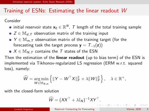
Training of ESNs: Estimating the linear readout W
Consider
initial reservoir state x0 ∈ RN , T length of the total training sample
Z ∈Md ,T observation matrix of the training input
Y ∈Mm,T observation matrix of the training target (for theforecasting task the target process y = T−1(z))
X ∈MN,T contains the T states of the ESN
Then the estimation of the linear readout (up to bias term) of the ESN isimplemented via Tikhonov-regularized LS regression (ERM w.r.t. squaredloss), namely:
W = argminW∈MN,m
‖Y −W>X‖2
F + λ‖W ‖2F
, λ ∈ R+,
with the closed-form solution
W = (XX> + λIN)−1XY>.
Lyudmila Grigoryeva ( University of Konstanz, Germany )Reservoir Computing for Forecasting Vienna, 2020 5
Universal reservoir system: Echo State Network (ESN)
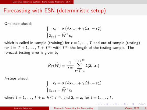
Forecasting with ESN (deterministic setup)
One step ahead: xt = σ (Axt−1 + γCzt + sζ)
zt+1 = W>xt ,
which is called in-sample (training) for t = 1, . . . ,T and out-of-sample (testing)for t = T + 1, . . . ,T + T tst with T tst the length of the testing sample. Theforecast testing error is given by
RT (W ) =1
T tst
T+T tst∑t=T+1
L(zt , zt)
h-steps ahead: xt = σ (Axt−1 + γC zt + sζ)
zt+1 = W>xt
where t = 1, . . . ,T + h, h ≤ T tst , and zt = zt for t = 1, . . . ,T .
Lyudmila Grigoryeva ( University of Konstanz, Germany )Reservoir Computing for Forecasting Vienna, 2020 6

Applications to stochastic processes
Stochastic setup
See [GO20] for the universal approximation properties of the ESNs and [GGO19]for their generalization error bounds for weakly dependent processes (non-sharp).Empirical question: how difficult is to find ESN which outperforms benchmarkcompetitors in the forecasting exercise.
Lyudmila Grigoryeva ( University of Konstanz, Germany )Reservoir Computing for Forecasting Vienna, 2020 7

Applications to stochastic processes
Application to stochastic processes
Task: forecasting realized (co)variances of intradaily (multiple) asset returns
Application of interest for financial mathematicians and financialeconometricians
Realized (co)variances exhibit the stylized features of financial time seriesalong with the features of long memory processes
Existing parametric models suffer from the curse of dimensionality whenapplied to high number of financial assets
Only short sample of historical observations is available (poor statisticalinference guarantees)
Time series show signs of extreme behaviour and regime changing (crisisevents)
Lyudmila Grigoryeva ( University of Konstanz, Germany )Reservoir Computing for Forecasting Vienna, 2020 8

Applications to stochastic processes
Realized variance of financial asset returns
Lyudmila Grigoryeva ( University of Konstanz, Germany )Reservoir Computing for Forecasting Vienna, 2020 9

Standard tools available
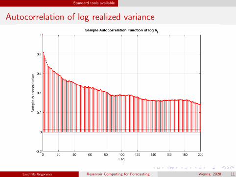
Signs of long memory behavior
Realized volatility time series exhibit long memory behavior features:
(i) Slow decay in lag k in sample auto-correlations
ρ(k) =1
n
n−|k|∑t=1
(zt − zn)(zt+|k| − zn) with zn =n∑
t=1
zt .
The decay of ρ(k) is hyperbolic with a rate k−α, 0 < α < 1 =⇒ non-summability.
(ii) Var(zn)→ 0 at a slower rate than n−1. Define
S2m = 1/(nm − 1)
nm∑i=1
(z (i−1)m,im − zn
)2, z t,m =
1
m
m∑j=1
zt+j , nm =⌈ nm
⌉.
Plot S2m against logm where m is the number of observations in the block.
(iii) R/S statistic [?]: Let yi =∑j
i=1 zi and define the adjusted range
R(t, k) := max0≤i≤k
yt+i − yt −i
k(yt+k − yt) − min
0≤i≤kyt+i − yt −
i
k(yt+k − yt).
Let z t,k = k−1∑t+ki=t+1 zi and define S(t, k) :=
√k−1
∑t+ki=t+1(zi − z t,k)2. The ratio
R(t,k)S(t,k)
is called the R/S statistic. As k →∞, log E [R/S ] ≈ a + H log k with H > 12
for short-range processes R/S behaves as√k, that is as k →∞, logR/S slope
1/2.Lyudmila Grigoryeva ( University of Konstanz, Germany )Reservoir Computing for Forecasting Vienna, 2020 10
Standard tools available
Autocorrelation of log realized variance
Lyudmila Grigoryeva ( University of Konstanz, Germany )Reservoir Computing for Forecasting Vienna, 2020 11
Standard tools available
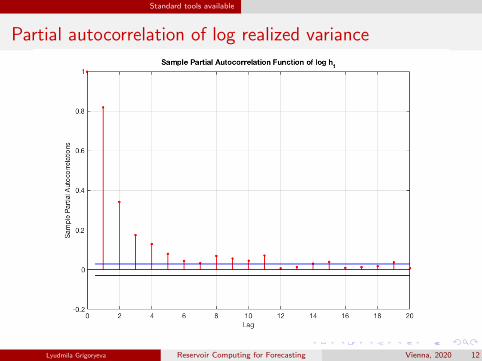
Partial autocorrelation of log realized variance
Lyudmila Grigoryeva ( University of Konstanz, Germany )Reservoir Computing for Forecasting Vienna, 2020 12

Standard tools available
Long memory processes
Standard characterisation of memory for time series process, which are second-orderstationary, builds upon properties of autocovariance functions γz(h), h ∈ Z or spectraldensity functions
fz(ω) =1
2n
∞∑h=−∞
γz(h) exp(−ihω), ω ∈ [−π, π]. (3)
Definition ([Ber94])
We say that a second-order stationary process zt , t ∈ Zhas long memory, if as |ω| → 0 fz(ω)→∞ or
∑h∈Z γz(h) =∞
has short memory, if as |ω| → 0 fz(ω)→ c or 0 <∑
h∈Z γz(h) <∞shows antipersistence, if as |ω| → 0 fz(ω)→ 0 or
∑h∈Z γz(h) = 0.
Using the equiv. characterization of processes [Ber94], one can define memory of a givenprocess using the behavior of γz(h), h ∈ Z and use in practice heuristics given above.
Definition
Let xt be a stationary process. xt is called a process with long memory, long rangedependence or strong dependence if there exists a constant cγ > 0 such that
lim|h|→∞
γz(h) = cγh−α, with α < 1. (4)
Lyudmila Grigoryeva ( University of Konstanz, Germany )Reservoir Computing for Forecasting Vienna, 2020 13

Standard tools available
ARFIMA process
An ARFIMA(p, d , q) (Granger and Joyeux [1980], Hosking [1981]) process isgiven by
Φ(L)(1− L)d(zt − ν) = Θ(L)εt , ε ∼ IID(0, σ2ε )
with
Φ(L) = 1− ϕ1L− ϕ2L− . . .− ϕpLp
Θ(L) = 1 + θ1L + θ2L + . . .+ θqLq
and the fractional difference operator (1− L)d defined by
(1− L)d =∞∑k=0
Γ(k − d)Lk
Γ(−d)Γ(k + 1)(5)
zt is invertible and stationary if all roots of Φ and Θ are outside the unit circleand |d | < 0.5. A stationary ARFIMA(p, d, q) process with d ∈ (0, 1
2 ) is a longmemory process. It is easy to verify that it that case, the condition (4) holds withα = 2d − 1.
Lyudmila Grigoryeva ( University of Konstanz, Germany )Reservoir Computing for Forecasting Vienna, 2020 14

Standard tools available
HAR [Cor09]
The daily return process rtt∈Z is given by
rt = σ(d)t εt , εt
IID∼ N(0, 1), t ∈ Z, (6)
with σ(d)t the daily integrated volatility. Idea: the hierarchical model for σ
(d)t using
a cascade of models for the partial latent volatilities at lower frequencies.
Introduce the daily partial realized volatilities σ(d)t such that σ
(d)t = σ
(d)t , the
weekly σ(w)t and monthly σ
(m)t latent partial volatilities. Assume they follow for all
t ∈ Z hold
σ(m)t+1m = α(m) + φ(m)RV
(m)t + ε
(m)t+1m, (7)
σ(w)t+1w = α(w) + φ(w)RV
(w)t + γ(w)Et [σ
(m)t+1m] + ε
(w)t+1w , (8)
σ(d)t+1d = α(d) + φ(d)RV
(d)t + γ(w)Et [σ
(w)t+1w ] + ε
(d)t+1d , (9)
where RV(d)t is the observed daily realized volatility, RV
(w)t = 1
5
∑4j=0 RV
(d)t−jd and
RV(m)t = 1
22
∑21j=0 RV
(d)t−jd , ε
(m)t+1m, ε
(w)t+1w , and ε
(d)t+1d are contemp. and serially
independent zero-mean innovations, which are left tail truncated.Lyudmila Grigoryeva ( University of Konstanz, Germany )Reservoir Computing for Forecasting Vienna, 2020 15

Standard tools available
HAR
The hierarchical approach yields
σ(d)t+1d = α + β(d)RV
(d)t + β(w)RV
(w)t + β(m)RV
(m)t + ε
(d)t+1d , t ∈ Z, (10)
where α = α(d) + γ(d)α(w) + γ(d)γ(w)α(m), β(d) = φ(d), β(w) = γ(d)φ(w), andβ(m) = γ(d)γ(w)φ(m). With
σ(d)t+1d = RV
(d)t+1d + ε
(d)t+1d , (11)
results in HAR model
RV(d)t+1 = α + β(d)RV
(d)t + β(w)RV
(w)t + β(m)RV
(m)t + εt+1, t ∈ Z, (12)
with εt+1 = ε(d)t+1d − ε
(d)t+1d with the temporal increments taken in the daily time
scale.HAR is a AR(22) model parametrized in a parsimonious way.Other versions of HAR model [AK16, AHO19]; produce superior quality forecastsin the calm market periods; suffer from losses of performance in periods of highvolatile market behavior; remain very strong competitors in the univariate andmultivariate setups [SSKM18].
Lyudmila Grigoryeva ( University of Konstanz, Germany )Reservoir Computing for Forecasting Vienna, 2020 16

Standard tools available
Pitfalls and tools
transforms preserving positivity (positive definiteness) of(co)volatilities - Box-Cox
choice of a particular loss function and regularization at the time oftraining which leads to good performance in terms of other evaluationcriteria used in the literature
residual (block) bootstrapping
changing the architecture as a response to regime switching
random ESNs with the Hedge boosting algorithm
Lyudmila Grigoryeva ( University of Konstanz, Germany )Reservoir Computing for Forecasting Vienna, 2020 17

Standard tools available
Box-Cox
Consider the original time series yt , t ∈ 1, . . . ,T of realized variances. Since ytis a non-negative process and its realizations often exhibit non-Gaussian behavior,one applies the Box-Cox transformation, namely for all t ∈ 1, . . . ,T
zt = fBC(yt ;λ) =
yλt − 1
λ, λ 6= 0,
ln yt , λ = 0(13)
and whose inverse we denote by gBC(zt , λ) = f −1BC (zt , λ) = yt . Based on zt ,
t ∈ 1, . . . ,T for each h ∈ 1, . . . , hmax construct the forecastzt+h := E[zt+h|Ft ]. The ultimate goal of the forecaster however is to obtain theforecast in the original representation yt+h := E[yt+h|Ft ]. The naıve approach ofobtaining a forecast as evaluation of the inverse function gBC(zt+h, λ) for convexfunctions by Jensen’s inequality leads to under-predictions asgBC(E[zt+h|Ft ], λ) ≤ E[gBC(zt+h;λ)|Ft ] and may result in incorrect rankings ofmodels.
Lyudmila Grigoryeva ( University of Konstanz, Germany )Reservoir Computing for Forecasting Vienna, 2020 18

Standard tools available
Forecast adjustment
Adjustment in [Tay17] based on the conditional expectation of a Taylor series
expansion of gBC(zt+h;λ) at zt+h. Denote by µ(k)t+h|t , k ∈ N, the k-th conditional
central moments of zt+h that is µ(1)t+h|t = E[zt+h|Ft ] and
µ(k)t+h|t = E[zkt+h|Ft ]− (µ
(1)t+h|t)
k for k > 1 and the full adjustment expression is
given by
E[gBC(zt+h;λ)|Ft ] = gBC(µt+h|t ;λ)
(1 +
∞∑k=1
g (k)(µt+h|t ;λ)µ(k)t+h|t
)(14)
where
g (k)(µt+h|t ;λ) =1− λ(k − 1)
k(1 + λµt+h|t)g (k−1)(µt+h|t ;λ), with g (0)(µt+h|t ;λ) = 0.
In particular, in the case of the logarithmic transformation (λ = 0 in (13)) the fulladjustment has the form
yt+h ≈ eµt+h|t
(1 +
∞∑k=1
1
k!µ
(k)t+h|t
)(15)
and for power transforms with λ = 1/n with n ∈ N, it is given by
yt+h ≈(
1 +µt+h|t
n
)n1 +n∑
k=1
(n − 1)!µ(k)t+h|t
k!(n − k)!nk−1(
1 + 1nµ
(k)t+h|t
) .
Lyudmila Grigoryeva ( University of Konstanz, Germany )Reservoir Computing for Forecasting Vienna, 2020 19
Standard tools available
Doob decomposition implications for forecasting
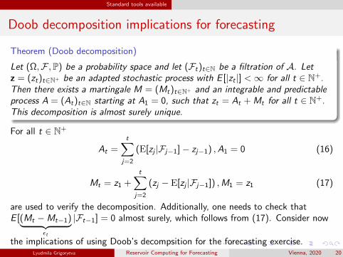
Theorem (Doob decomposition)
Let (Ω,F ,P) be a probability space and let (Ft)t∈N be a filtration of A. Letz = (zt)t∈N+ be an adapted stochastic process with E [|zt |] <∞ for all t ∈ N+.Then there exists a martingale M = (Mt)t∈N+ and an integrable and predictableprocess A = (At)t∈N starting at A1 = 0, such that zt = At + Mt for all t ∈ N+.This decomposition is almost surely unique.
For all t ∈ N+
At =t∑
j=2
(E[zj |Fj−1]− zj−1) ,A1 = 0 (16)
Mt = z1 +t∑
j=2
(zj − E[zj |Fj−1]) ,M1 = z1 (17)
are used to verify the decomposition. Additionally, one needs to check thatE [(Mt −Mt−1)︸ ︷︷ ︸
εt
|Ft−1] = 0 almost surely, which follows from (17). Consider now
the implications of using Doob’s decompsition for the forecasting exercise.Lyudmila Grigoryeva ( University of Konstanz, Germany )Reservoir Computing for Forecasting Vienna, 2020 20
Forecasting with ESN
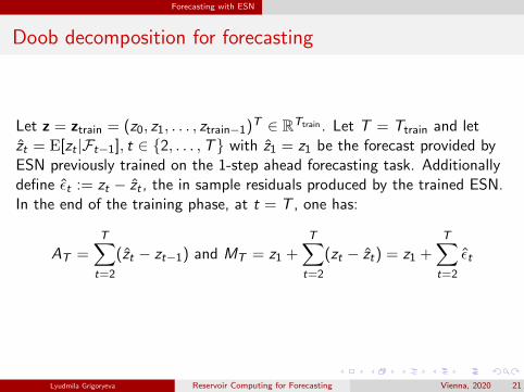
Doob decomposition for forecasting
Let z = ztrain = (z0, z1, . . . , ztrain−1)T ∈ RTtrain . Let T = Ttrain and letzt = E[zt |Ft−1], t ∈ 2, . . . ,T with z1 = z1 be the forecast provided byESN previously trained on the 1-step ahead forecasting task. Additionallydefine εt := zt − zt , the in sample residuals produced by the trained ESN.In the end of the training phase, at t = T , one has:
AT =T∑t=2
(zt − zt−1) and MT = z1 +T∑t=2
(zt − zt) = z1 +T∑t=2
εt
Lyudmila Grigoryeva ( University of Konstanz, Germany )Reservoir Computing for Forecasting Vienna, 2020 21

Forecasting with ESN
Implementation
Let Nr be the number of bootstrap replications. We construct Nr random subsamples ofresiduals at the time of training, each of length hmax, namely
E (j) =(ε
(j)1 , ε
(j)2 , . . . , ε
(j)hmax
), j = 1, . . . ,Nr.
h = 1:
z(j)T+1 = AT+1 + M
(j)T+1, j = 1, . . . ,Nr ,with
AT+1 =T∑t=2
(zt − zt−1)︸ ︷︷ ︸AT
+(zT+1 − zT )
M(j)T+1 = z1 +
T∑t=2
(zt − zt)︸ ︷︷ ︸MT
+ (zT+1 − zT+1)︸ ︷︷ ︸not available εT+1
=: MT + ε(j)1
with zT+1 provided by the ESN.
Lyudmila Grigoryeva ( University of Konstanz, Germany )Reservoir Computing for Forecasting Vienna, 2020 22

Forecasting with ESN
h = 2:
z(j)T+2 = A
(j)T+2 + M
(j)T+2, j = 1, . . . ,Nr ,with
A(j)T+2 = AT+1 + (zT+2 − zT+1)
M(j)T+2 = M
(j)T+1 + ε
(j)2
until h = hmax:
z(j)T+hmax
= A(j)T+hmax
+ M(j)T+hmax
, j = 1, . . . ,Nr ,with
A(j)T+hmax
= AT+hmax−1 + (zT+hmax − zT+hmax−1)
M(j)T+hmax
= M(j)T+hmax−1 + ε
(j)hmax
Finally construct forecasts as:
zesnt+h =
1
Nr
Nr∑j=1
z(j)t+h, h = 1, . . . , hmax, j = 1, . . . ,Nr .
z(j)T+1 = zesn
T+1 + ε(j)1
...
z(j)T+hmax
= zesnT+hmax
+ ε(j)hmax
Lyudmila Grigoryeva ( University of Konstanz, Germany )Reservoir Computing for Forecasting Vienna, 2020 23
Forecasting with ESN Forecasting with ESNs
Forecasting with ESNs
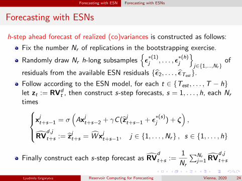
h-step ahead forecast of realized (co)variances is constructed as follows:
Fix the number Nr of replications in the bootstrapping exercise.
Randomly draw Nr h-long subsamplesε∗(1)j , . . . , ε
∗(h)j
j∈1,...,Nr
of
residuals from the available ESN residuals ε2, . . . , εTest.Follow according to the ESN model, for each t ∈ Test , . . . ,T − hlet zt := RVd
t , then construct s-step forecasts, s = 1, . . . , h, each Nr
timesxjt+s−1 = σ
(Axjt+s−2 + γC (zjt+s−1 + ε
∗(s)j ) + ζ
),
RVd ,j
t+s := zjt+s = W xjt+s−1, j ∈ 1, . . . ,Nr , s ∈ 1, . . . , h
Finally construct each s-step forecast as RVd
t+s :=1
Nr
∑Nrj=1 RV
d ,j
t+s
Lyudmila Grigoryeva ( University of Konstanz, Germany )Reservoir Computing for Forecasting Vienna, 2020 24
Forecasting with ESN Forecasting with ESNs
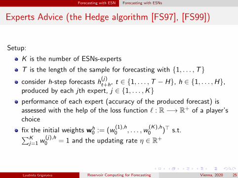
Experts Advice (the Hedge algorithm [FS97], [FS99])
Setup:
K is the number of ESNs-experts
T is the length of the sample for forecasting with 1, . . . ,Tconsider h-step forecasts h
(j)t+h, t ∈ 1, . . . ,T − H, h ∈ 1, . . . ,H,
produced by each jth expert, j ∈ 1, . . . ,Kperformance of each expert (accuracy of the produced forecast) isassessed with the help of the loss function ` : R −→ R+ of a player’schoice
fix the initial weights wh0 := (w
(1),h0 , . . . ,w
(K),h0 )> s.t.∑K
j=1 w(j),h0 = 1 and the updating rate η ∈ R+
Lyudmila Grigoryeva ( University of Konstanz, Germany )Reservoir Computing for Forecasting Vienna, 2020 25
Forecasting with ESN Forecasting with ESNs
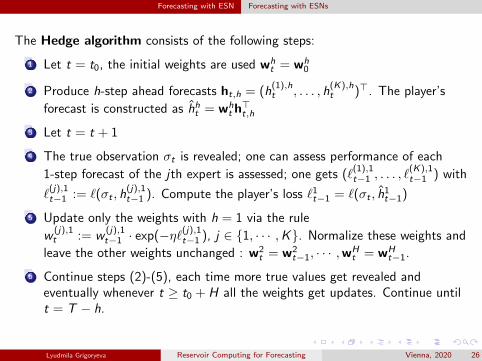
The Hedge algorithm consists of the following steps:
1 Let t = t0, the initial weights are used wht = wh
0
2 Produce h-step ahead forecasts ht,h = (h(1),ht , . . . , h
(K),ht )>. The player’s
forecast is constructed as hht = wht h>t,h
3 Let t = t + 1
4 The true observation σt is revealed; one can assess performance of each
1-step forecast of the jth expert is assessed; one gets (`(1),1t−1 , . . . , `
(K),1t−1 ) with
`(j),1t−1 := `(σt , h
(j),1t−1 ). Compute the player’s loss `1
t−1 = `(σt , h1t−1)
5 Update only the weights with h = 1 via the rule
w(j),1t := w
(j),1t−1 · exp(−η`(j),1
t−1 ), j ∈ 1, · · · ,K. Normalize these weights and
leave the other weights unchanged : w2t = w2
t−1, · · · ,wHt = wH
t−1.
6 Continue steps (2)-(5), each time more true values get revealed andeventually whenever t ≥ t0 + H all the weights get updates. Continue untilt = T − h.
Lyudmila Grigoryeva ( University of Konstanz, Germany )Reservoir Computing for Forecasting Vienna, 2020 26
Empirical study Data
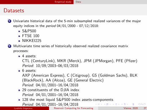
Datasets
1 Univariate historical data of the 5-min subsampled realized variances of the major
equity indices in the period 04/01/2000 - 07/12/2018:
S&P500FTSE 100NIKKEI225
2 Multivariate time series of historically observed realized covariance matrix
processes:
4 assets:CTL (CenturyLink), MKR (Merck), JPM (JPMorgan), PFE (Pfizer)Period: 10/09/2003–06/03/20186 assets:AXP (American Express), C (Citigroup), GS (Goldman Sachs), BLK(BlackRock), AA (Alcoa), GE (General Electric)Period: 04/01/2001–16/04/201829 constituents of the DJIA indexPeriod: 04/01/2001–16/04/2018128 the most liquid S&P500 index assets-componentsPeriod: 04/01/2001–16/04/2018
Lyudmila Grigoryeva ( University of Konstanz, Germany )Reservoir Computing for Forecasting Vienna, 2020 27
Empirical study Forecast performance evaluation
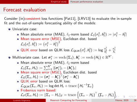
Forecast evaluation
Consider (in)consistent loss functions [Pat11], [LRV13] to evaluate the in-samplefit and the out-of-sample forecasting ability of the models:
Univariate case:
Mean absolute error (MAE), `1-norm based L1(σ2t , h
2t ) := |σ2
t − h2t |
Mean square error (MSE), Euclidean dist. based
L2(σ2t , h
2t ) :=
(σ2t − h2
t
)2
QLIK error based on QLIK loss LQLIK (σ2t , h
2t ) := log
σ2t
h2t
+σ2t
ht
Multivariate case. Let σvt := vech (Σt) ,hv
t := vech (Ht) ∈ RN∗ :
Mean absolute error (MAE), `1-norm based
L1(Σt ,Ht) :=∑N∗
i=1 |(σvt )i − (hv
t )i |Mean square error (MSE), Euclidean dist. basedLE (Σt ,Ht) := (σv
t − hvt )>(σv
t − hvt )
QLIK error based on QLIK loss:LQLIK (Σt ,Ht) := log detHt + trace
Ht−1Σt
Frobenius norm based:LF (Σt ,Ht) := ‖Σt − Ht‖F = trace
(Σt − Ht)
> (Σt − Ht)
Lyudmila Grigoryeva ( University of Konstanz, Germany )Reservoir Computing for Forecasting Vienna, 2020 28
Empirical study Forecast performance evaluation
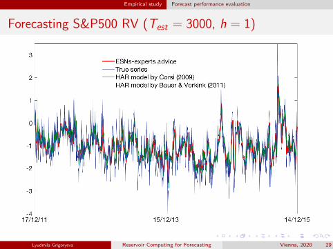
Forecasting S&P500 RV (Test = 3000, h = 1)
Lyudmila Grigoryeva ( University of Konstanz, Germany )Reservoir Computing for Forecasting Vienna, 2020 29

Empirical study Forecast performance evaluation
Forecasting S&P500 RV (Test = 3000, h = 30)
Lyudmila Grigoryeva ( University of Konstanz, Germany )Reservoir Computing for Forecasting Vienna, 2020 30
Empirical study Forecast performance evaluation
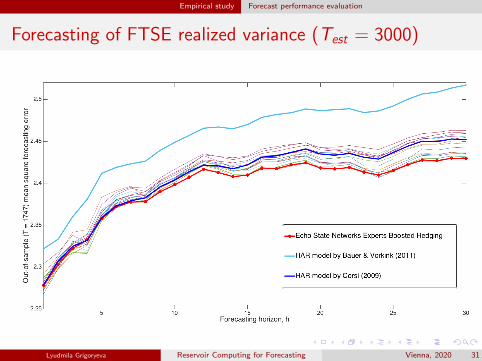
Forecasting of FTSE realized variance (Test = 3000)
Lyudmila Grigoryeva ( University of Konstanz, Germany )Reservoir Computing for Forecasting Vienna, 2020 31
Empirical study Forecast performance evaluation
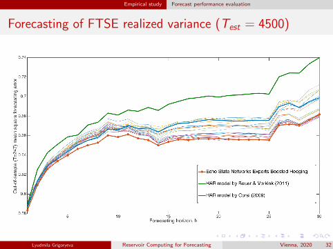
Forecasting of FTSE realized variance (Test = 4500)
Lyudmila Grigoryeva ( University of Konstanz, Germany )Reservoir Computing for Forecasting Vienna, 2020 32
Empirical study Forecast performance evaluation
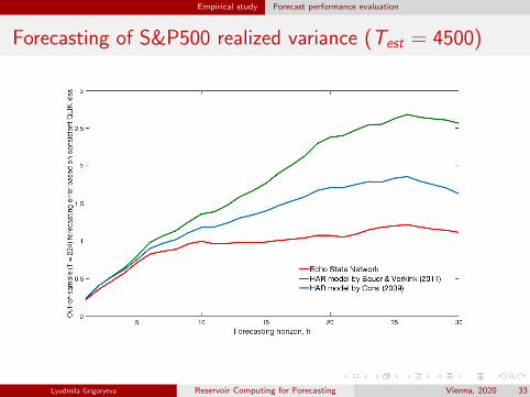
Forecasting of S&P500 realized variance (Test = 4500)
Lyudmila Grigoryeva ( University of Konstanz, Germany )Reservoir Computing for Forecasting Vienna, 2020 33

Empirical study Forecast performance evaluation
Forecasting of NIKKEI realized variance (Test = 4500)
Lyudmila Grigoryeva ( University of Konstanz, Germany )Reservoir Computing for Forecasting Vienna, 2020 34

Empirical study Forecast performance evaluation
Forecasting of NIKKEI realized variance (Test = 4500)
Lyudmila Grigoryeva ( University of Konstanz, Germany )Reservoir Computing for Forecasting Vienna, 2020 35
Empirical study Forecast performance evaluation
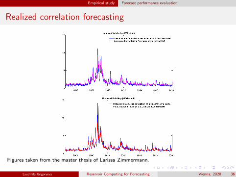
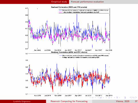
Realized correlation forecasting
Figures taken from the master thesis of Larissa Zimmermann.
Lyudmila Grigoryeva ( University of Konstanz, Germany )Reservoir Computing for Forecasting Vienna, 2020 36
Empirical study Forecast performance evaluation
Lyudmila Grigoryeva ( University of Konstanz, Germany )Reservoir Computing for Forecasting Vienna, 2020 37
Empirical study Forecast performance evaluation
Empirical results
ESN outperforms state-of-the-art models for realized volatility inforecasting tasks
ESN trained on a given training dataset of one given index is showedto perform well in forecasting of a number of other indices
Lyudmila Grigoryeva ( University of Konstanz, Germany )Reservoir Computing for Forecasting Vienna, 2020 38

References
References I
Francesco Audrino, Chen Huang, and Okhrin Ostap.
Flexible HAR model for realized volatility.Studies in Nonlinear Dynamics and Econometrics, 23(3), 2019.
F. Audrino and S.D. Knaus.
Lassoing the HAR model: A model selection perspective on realized volatility dynamics.Econometric Reviews, 35(8-10):1485–1521, 2016.
George E. P. Box and D. R. Cox.
An analysis of transformations (with discussion).Journal of the Royal Statistical Society. Series B, 26:211–246, 1964.
Jan Beran.
Statistics for Long-Memory Processes.CRC Press, 1994.
Nicolo Cesa-Bianchi and Gabor Lugosi.
Prediction, Learning, and Games.Cambridge University Press, 2006.
F. Corsi.
A simple approximate long-memory model of realized volatility.Journal of Financial Econometrics, 7(2):174–196, 2009.
Yoav Freund and Robert E. Schapire.
A decision-theoretic generalization of online learning and an application to boosting.Journal of Computer and System Sciences, 55(1):119–139, 1997.
Lyudmila Grigoryeva ( University of Konstanz, Germany )Reservoir Computing for Forecasting Vienna, 2020 39

References
References II
Yoav Freund and Robert E. Schapire.
Adaptive game playing using multiplicative weights.Games and Economic Behavior, 29:79–103, 1999.
Lukas Gonon, Lyudmila Grigoryeva, and Juan-Pablo Ortega.
Risk bounds for reservoir computing.Preprint, 2019.
Sılvia Goncalves and Nour Meddahi.
Box–Cox transforms for realized volatility.Journal of Econometrics, 160:129–144, 2011.
Lukas Gonon and Juan-Pablo Ortega.
Reservoir computing universality with stochastic inputs.IEEE Transactions on Neural Networks and Learning Systems, 31(1):100–112, 2020.
Sebastien Laurent, J. Rombouts, and Francesco Violante.
On loss functions and ranking forecasting performances of multivariate volatility models.Journal of Econometrics, 173(1):1–10, 2013.
A. J. Patton.
Volatility forecast comparison using imperfect volatility proxies.Journal of Econometrics, 160(1):246–256, 2011.
Tommaso Proietti and Helmut Lutkepohl.
Does the Box-Cox transformation help in forecasting macroeconomic time series?2011.
Lyudmila Grigoryeva ( University of Konstanz, Germany )Reservoir Computing for Forecasting Vienna, 2020 40

References
References III
Efthymia Symitsi, Lazaros Symeonidis, Apostolos Kourtis, and Raphael Markellos.
Covariance forecasting in equity markets.Journal of Banking & Finance2, 96:153–168, 2018.
Nick Taylor.
Realised variance forecasting under Box-Cox transformations.International Journal of Forecasting, 33:770–785, 2017.
Lyudmila Grigoryeva ( University of Konstanz, Germany )Reservoir Computing for Forecasting Vienna, 2020 41