Embed Size (px)
Citation preview
Stability Region Based Robust ControllerSynthesis
Robuste Reglersynthese auf Grundlage von stabilisierendenParameterräumen
Von der Fakultät für Maschinenwesen der Rheinisch-WestfälischenTechnischen Hochschule Aachen zur Erlangung des akademischen
Grades eines Doktors der Ingenieurwissenschaften genehmigteDissertation
vorgelegt vonFrank Schrödel
Berichter: Univ.-Prof. Dr.-Ing. Dirk AbelUniv.-Prof. Dr. med. Dr.-Ing. Klaus Steffen Leonhardt
Tag der mündlichen Prüfung: 09. Februar 2016
Diese Dissertation ist auf den Internetseiten der Universitätsbibliothekonline verfügbar.

II
III
Erfahrung heißt, seine Grenzen kennen;Weisheit heißt, seine Grenzen respektieren.
—Experience means, knowing your boundaries.Wisdom means, respecting your boundaries.
Hans-Jürgen Quadbeck-Seeger

IV
Preface V
PrefaceFirst, I would like to thank Prof. Dr.-Ing. D. Abel for his supportand confidence during my work at the institute. Moreover, I wouldlike to thank Prof. Dr. med. Dr.-Ing. Klaus Steffen Leonhardt forco-supervising the dissertation and his valuable feedback. Furthermore,I would like to thank my colleges at the IRT for their friendship, helpand support. Especially, the discussions with J. Maschuw and L. Pytawere really inspiring. I also would like to thank all my students for theirsupport during this fascinating project. With regard to the practicalexperiments, I would like to thank B. Alrifaee, M. Brüderlin, T. Engel-hardt, M. Reiter, D. Rüschen and D. Zöller.Special thanks goes to Dr.-Ing. W. Sienel and Dr.-Ing. T. Bünte, whohave supported my work by sharing their research results during thelast years. The main important external supporters were Dr.-Ing. N.Bajcinca, R. Vosswinkel and Prof. Dr.-Ing. M. T. Söylemez - thanksfor the great discussions! Additionally, I would like to thank my for-mer professors from the O.v.G. University Magdeburg, who showed andshared with me the beauty of control engineering science.Moreover, I would like to thank my former fellow students Nadine, René,Sebastian and Tobias for their continued support and friendship. I alsowould like to thank Katharina, Carl and all my other friends from Jenafor their friendship and support enabling me to survive the time spentworking on my PhD. Thank you for the amazing trips over the last fewyears! Last but not least, I would like to give many heartfelt thanksto Carina, my sister and my parents. Without them, this work wouldnever have been possible.The present dissertation is an outcome of my research work at the In-stitute of Automatic Control at the RWTH Aachen University. In thiscontext, the contribution from the German Research Foundation (DFG)in terms of financial support for the project (AB 65/2-3) is acknowl-edged.
Aachen, October 2015 Frank Schrödel
VI Contents
Contents
Symbols and Abbreviations VIII
1 Introduction 1
2 Stability region calculation 52.1 Root locus-based preliminaries . . . . . . . . . . . . . . 52.2 General problem statement . . . . . . . . . . . . . . . . 152.3 Parameter space approach . . . . . . . . . . . . . . . . . 17
2.3.1 Single-loop PID control for delay-free systems . . 182.3.2 Single-loop PID control for delay systems . . . . 292.3.3 MIMO and mesh-loop PID control . . . . . . . . 392.3.4 State space representation-based control . . . . . 49
2.4 Hermite-Biehler theorem-based approach . . . . . . . . . 542.4.1 Single-loop PID control for delay-free systems . . 552.4.2 Single-loop PID control for delay systems . . . . 60
2.5 Alternative Approaches . . . . . . . . . . . . . . . . . . 642.5.1 Dual locus approach . . . . . . . . . . . . . . . . 642.5.2 Θ- and B-stability-based approach . . . . . . . . 672.5.3 Describing function-based approach . . . . . . . 722.5.4 Routh-Hurwitz-based approach . . . . . . . . . . 74
2.6 Lyapunov stability-based approach . . . . . . . . . . . . 752.6.1 Continuous LTI systems . . . . . . . . . . . . . . 762.6.2 Continuous LTI systems with delay . . . . . . . . 832.6.3 Discrete-Time LTI systems . . . . . . . . . . . . 872.6.4 Advanced system classes . . . . . . . . . . . . . . 922.6.5 Controllability and observability mapping . . . . 96
2.7 Probabilistic-based approach . . . . . . . . . . . . . . . 97
3 Robustness-based synthesis 1003.1 Analysis step . . . . . . . . . . . . . . . . . . . . . . . . 101
3.1.1 Delay parameter region charts . . . . . . . . . . 1013.1.2 System parameter region charts . . . . . . . . . . 106
Contents VII
3.1.3 Advanced system classes . . . . . . . . . . . . . . 1143.2 Test set-based robust controller synthesis . . . . . . . . 115
3.2.1 Interval polynomials . . . . . . . . . . . . . . . . 1153.2.2 Polynomials with affine dependencies . . . . . . . 1203.2.3 Polynomials with multilinear dependencies . . . 1293.2.4 Quasi-polynomials with uncertainties . . . . . . . 1363.2.5 Outlook . . . . . . . . . . . . . . . . . . . . . . . 140
3.3 LTV system stability-based approach . . . . . . . . . . . 1433.4 Robustness verification techniques . . . . . . . . . . . . 148
4 Performance-based synthesis 1504.1 Parameter space shrinking . . . . . . . . . . . . . . . . . 1514.2 Start point calculation . . . . . . . . . . . . . . . . . . . 1574.3 Time domain-based optimization . . . . . . . . . . . . . 162
4.3.1 Performance maps . . . . . . . . . . . . . . . . . 1624.3.2 Automatic optimization . . . . . . . . . . . . . . 164
4.4 Frequency domain-based optimization . . . . . . . . . . 1704.4.1 Performance maps . . . . . . . . . . . . . . . . . 1704.4.2 Loop shaping . . . . . . . . . . . . . . . . . . . . 176
4.5 Eigenvalue-based analysis and optimization . . . . . . . 1824.6 Performance verification techniques . . . . . . . . . . . . 187
5 Implementation & Application 1885.1 Vacuum thermal evaporation process . . . . . . . . . . . 1915.2 Rijke tube . . . . . . . . . . . . . . . . . . . . . . . . . . 1965.3 Ventricular assist device . . . . . . . . . . . . . . . . . . 1985.4 Aeroelastic flight application . . . . . . . . . . . . . . . 2015.5 Pendulum . . . . . . . . . . . . . . . . . . . . . . . . . . 2075.6 Advanced drive assistant systems . . . . . . . . . . . . . 2125.7 Multicopter control . . . . . . . . . . . . . . . . . . . . . 220
6 Conclusion and outlook 224
Bibliography 226
7 Involved Students 257
8 Personal Publications 262
VIII Symbols and Abbreviations
Symbols and Abbreviations
Latin letters
a0, a1, . . . , am Real coefficients of the polynomial A(s, . . . )ac,0, ac,1, . . . , ac,m Real coefficients of the polynomial AC(s, . . . )az� Highest real coefficient of the A polynomialaz� Highest imaginary coefficient of the A polynomiala0
0, a01, . . . , a0
m Real coefficients of the polynomial A0(s, . . . )aΔ
0 , aΔ1 , . . . , aΔ
m Real coefficients of the polynomial AΔ(s, . . . )a0, a1, . . . , am Real coefficients of the characteristic polynomial δ(s, . . . )a0, a1, . . . , am Real coefficients of the system matrix AA(s, . . . ) Numerator polynomial of the plant GP (s, . . . )A Auxiliary polynomial A = A(s, . . . )A0 Real certain coefficients of the polynomial A(s, . . . )AΔ Real uncertain coefficients of the polynomial A(s, . . . )AC(s, . . . ) Real coefficients of the numerator of the controller GC(s)A(s, . . . ) Real coefficients of the open-loop polynomial by using a
ideal PID controllerAM Amplitude marginA AreaA System matrixAk Closed-loop system matrixAτ System matrix of the delayed statesAk(k) Closed-loop discrete-time system matrixAσ Closed-loop system matrix for switching systemsA(t) Time-varying system matrixA Nominal system matrixA Set of polynomial coefficientsA� Set of polynomial coefficients in form of a boxb0, b1, . . . Real coefficients of the polynomial B(s, . . . )bc,0, bc,1, . . . , bc,m Real coefficients of the polynomial BC(s, . . . )bz� Highest real coefficient of the B polynomialbz� Highest imaginary coefficient of the B polynomialb0
0, b01, . . . , b0,m Real coefficients of the polynomial B0(s, . . . )
bΔ0 , bΔ
1 , . . . , bΔm Real coefficients of the polynomial BΔ(s, . . . )
Symbols and Abbreviations IX
b Release constantb Input vectorB(s, . . . ) Open-loop numerator (using an ideal PID sB(s, . . . ))B0 Real certain coefficients of the polynomial B(s, . . . )BΔ Real uncertain coefficients of the polynomial B(s, . . . )B(s, . . . ) Real coefficients in the denominator of GP (s, . . . )BC(s, . . . ) Real coefficients in the denominator of GC(s, . . . )B(U) Describing function∂B = |B(jω)| Bound of the desired amplitude responseB Desired amplitude responseB Real coefficients in the denominator of the plant in the
case of mesh-loop controlc CRB auxiliary variable by using a real PID controllerc Heat capacitycp Specific heat at constant pressurecv Specific heat at constant volumecW Air resistancec Output vectorc(k) Equality boundary conditionsC Heat capacity ratiod Disturbance signald0, d1, . . . , dnD Real coefficients of the polynomial D(s, . . . )d�� Element of the diagonal matrix Dd Number of linear combinations of independent interval
polynomialsd Search directionD Damping factorD(s, . . . ) Auxiliary polynomial in the case of mesh-loop controlD(s, . . . ) Polynomial for mesh-loop control (D(s) = D(s)eτs)D Diagonal matrixe Control derivationE Control derivation in the frequency domainE Coupling matrix of a descriptor systemf� Auxiliary polynomials for the CRB calculationf�
i Right eigenvectorf�
i Left eigenvectorf FrictionFi(s) Fixed polynomialFkP Set which contains all possible stringsF ∗
kPSet which contains the feasible string
F∂Θ Bounding function of the Θ-area
X Symbols and Abbreviations
F ForceF Matrix for the CRB calculationF k Delay type matrixg Gravity constantg Heat release gainG0(s, . . . ) Transfer function of the open-loop systemGC(s, . . . ) Transfer function of the controllerGCA (s, . . . ) Auxiliary controllerGd(s, . . . ) Denominator of the transfer function G(s, . . . )GP (s, . . . ) Transfer function of the plant (GP (s) = A(s)/B(s))Gn(s, . . . ) Numerator of the transfer function G(s, . . . )G Auxiliary matrixh Number of uncertain plant parametersh(ω,q) Function for singular frequency calculation in delay caseh Enthalpyh(k) Inequality boundary conditionsH�� Transfer function of a pre-compensatorH1−n HeaterH Hurwitz matrixi Control variableit Sequence of signum valuesi CurrentIi(s) Interval polynomials��, �(�) Imaginary part of a complex numberIp CRB intersection pointI Interlacing property stringIi(s) Line segmentI Identity matrixj Control variablej Imaginary unitJ Cost functionJIAE Cost function of integral absolute errorsJISE Cost function of integral square errorsJIT EA Cost function of integral time errorsJLQR Cost function of a linear quadratic regulatorJ Moment of inertiaJ Jacobian matrixJ Matrix for the matrix multiplication methodkP , kI , kD Proportional, integral, differential gain for PID controllerkPA , kIA , kDA Gains for PID auxiliary controllerk0
I,� Intersection point of the CRB
Symbols and Abbreviations XI
k Actual time step in a difference equationk Vector of the controller parameterskk Vector of the controller parameters at each iteration stepk State feedback gain vectorK System gainK Heat flow constantKi Kharitonov polynomial iK Controller parameter setKδi Controller parameter set which stabilizes the system δi(s)KQ Controller parameter set which stabilizes the whole op-
erating domain Ql Control variable for the CRB calculationl(δ) Number of roots in the OLHPl Number of uncertain parametersL(s, . . . ) Magnitude condition for the HBT in the delay caseL LengthL Regular matrixL(k,s,λ) Optimization problemm Degree of the numerator polynomial A(s, . . . )m0 Number of roots of A(s, . . . ) in the originmD Degree of polynomial D(s, . . . )mI Number of roots s = jω of A(s, . . . ) with ωj �= 0mR Number of roots of A(s, . . . ) in the ORHPmI Number of mI roots with an additional specificationm MassMa Mach numberM Highest power of s in δ(ω, k, q)MS Maximum sensitivityM Auxiliary matrix for the Lyapunov stability mappingn Degree of B(s, . . . ), δ(s, . . . ) and dimension of A(s, . . . )n′ Max. degree for zmin calculation (n′ = max(n,m + 2))N Highest power of es in δ(ω, k, q)NU Number of unstable rootso Number of delaysO Calculation complexityp Number of zeros of A(s) in the ORHPp�,� Element of the Lyapunov matrix Pp1−3 Auxiliary polynomial for the Θ- and B-stability mappingp(ω) Polynomial for the CRB calculation for the Dual locusp PressurePel Electrical power
XII Symbols and Abbreviations
P r Projector matrixPS Heating powerP Lyapunov matrixP Nominal Lyapunov matrixP C Controllability gramianP O Observability gramianP Plant parameter spaceq�,� Element of the matrix Qqi Plant parameterq Vector of plant parametersQ CrucibleQi(s) A polynomial with only odd or even power of sQB B-stable region in the parameter domainQΘ Θ-stable region in the parameter domainQ HeatQ Heat flowQ Solution of the general Lyapunov equationQC Controllability matrixQO Observability matrixQ Weighting matrix of the statesQ Operating domain of the plant parametersQki Edges in the test set QT
QT Worst case set of system parametersr Control variabler(δ) Number of roots in the ORHPr(ω) Variable for the CRB calculation for the dual locusr Stability radiusri Residuum iri Residuum vectorR Upper bound of singular frequency intervalR� Entry in the Routh-Hurwiz arrayR(jω) Inverse weighting function W3��, �(�) Real part of a complex number�∞
� Real part of a complex number for s → ∞Rd Acoustic reflection coefficients - downstreamRu Acoustic reflection coefficients - upstreamR Real coefficient matrixR Weighting matrix of the manipulated variableR Resolvent matrixR Set of Kharitonov segmentsR Set of real numbers
Symbols and Abbreviations XIII
R+ Set of positive real numbers
R+0 Set of positive real numbers inclusive zero
s Complex Laplace variablesi Polesi Approximated poles Perpetuated eigenvalueS(jω) Sensitivity functionS(jω) Inverse weighting function of the sensitivity functionS Kharitonov segments Slag variableS Diagonal matrix of slag variablest Time in secondsti Control variableT Time constantT (jω) Complementary sensitivity functionT (jω) Inverse weighting for complementary sensitivity functionTK Trust regionTn Time constant of a PI controllerTP Filter constant of the differential part for real PIDTS Sampling timeTz,w(jω) Transfer function matrix for the H-Infinity controllerTτ Stability critical time constantT TemperatureTS,1−n Temperature sensorT Transformation matrixT Test setTE Test set build by the edges of the operating domainTS Worst case test setu Manipulated variableu EigenvectorUi(s) Anti-Hurwitz polynomial only with poles in the ORHPv Velocityv EigenvectorV Lyapunov functionV Volume flowV Optimal velocity functionw Set pointW (ω) Auxiliary polynomial for the direct methodWKS Weighting matrix for the H-Infinity controller synthesisWS Weighting matrix of the sensitivity functionWT Weighting matrix for complementary sensitivity function
XIV Symbols and Abbreviations
x Positionx State vectorx Approximated state vectorX Real coefficient matrixy Plant outputY Real coefficient matrixz Auxiliary matrix for the CRB calculationzmin Minimum number of singular frequenciesz Point in the Nyquist domainzω Imaginary part of a point in the Nyquist domainzσ Real part of a point in the Nyquist domainz Complex variable in the z-domainZ Signal for the H-Infinity controller synthesisZ Hamiltonian matrix
Greek letters
αε ε-pseudo spectrumα Control variableβ Auxiliary variableχ Driver sensitivityδ(s, . . . ) Characteristic polynomialδ(s, . . . ) Polynomial familyδ(s, . . . ) Auxiliary polynomial for the IRB calculationΔ Distanceε Auxiliary variableε Emissivityη Auxiliary variableγ RRB asymptoteΓ Slop of the streetι Thrust coefficientκ Auxiliary variableλ Parametrization of a line segment and a matrix coverλh Lagrange multiplier (inequality constrains)λc Lagrange multiplier (equality constrains)μ Leading principle minors∇k Nabla operator∇2
kkL Hessian matrixν Real constants for CRB study in the delay caseω Angular frequency
Symbols and Abbreviations XV
ωc Crossover frequencyωs,t Singular frequency number tωτ Crossing frequencyωs Vector of singular frequenciesΩ Set of critical frequencies∂ Small variationφ Real constants for CRB study in the delay caseΦ CRB calculation matrixΦ State transition matrixϕM Phase marginϕ Pendulum angular� DiameterΨ Part of a cost functionρ Density� Acoustic velocityσ Real part of a variableσ0 Largest real part of all polesσi Imaginary signatureσr Real signatureς Stefan-Boltzmann constantτ Time delayτM Delay marginττ Crossing delayΘ Θ-stability area in the Nyquist domain∂Θ Θ-stability bound in the Nyquist domainϑ Angle of attackυ Complex Laplace variableΥ Heat flow on the thermal conductivityξ Auxiliary variable for the B-stable mappingξd Denominator of the auxiliary variable control setup ξΞ(ω) Angle of Nyquist intersection points and neg. real axisζ Auxiliary variable
Operators
�e Even polynomial�M Marginally stable candidate point on α�o Odd polynomial�� Over-approximation of the operating domain in form of
a hyper rectangle
XVI Symbols and Abbreviations
�α Candidate point α�β Candidate point β�′ Transformed Parameter�− Minimum value of the variable ��+ Minimum value of the variable ��∗ Fixed value of the variable �(�)ᵀ Transposed value�H Conjugate transposed value� First derivative with respect to time� Second derivative with respect to time� Arithmetic mean value� Set of edges of the operating domain|�| Magnitude||�||2 H-2 norm||�||F Frobenius norm�� Floor function�� Ceiling function〈�〉 Scalar product⊗ Kronecker product∠(�) Phase� ≺ 0 Negative definiteness� � 0 Positive semi-definitenessatan(�) Arctangentco� Convex matrix coverconv� Convex hullcos(�) Cosine functiondet(�) Determinate∈ � Element in set �/∈ � Element not in set �ev� Eigenvalue of �mod � Modulus functionRes� Resultant functionsin(�) Sinus functionsup� Supremum functionTr� Trace functiontrig(�) Either sin(�) or cos(�)vec(�) Vector which rearranges the matrix entries column-wise0 Zero vector∅ Empty set∀ For all∞ Infinity
Symbols and Abbreviations XVII
Abbreviations
CATS Chair for computational analysis of technical systems, RWTHAachen University
CFD Computational fluid dynamicCRB Complex root boundaryCTCR Cluster treatment of characteristic rootsFPV Four property validationFTE Frozen time eigenvaluesHBT Hermite-Biehler theoremHODS High order delay systemHOS High order systemi.c.r Instantaneous center of rotationIMC Internal model controlIQC Internal quality controlIRB Infinite root boundaryIRT Institute of automatic control, RWTH Aachen UniversityISE Integral square errorLARC PETW tests for loads, aeroelastics and robust active controlLMI Linear matrix inequalityLPV Linear parameter variantLQR Linear quadratic controllerLTI Linear time-invariantOLHP Open left half-planeOP Operating pointORHP Open right half-planePETW Pilot European transonic wind tunnelPID Controller with proportion, integral and derivative behaviorPSA Parameter space approachROM Reduced order modelRRB Real root boundaryRT Root tendencySISO Single input single outputSODS Second order delay systemSOS Second order systemSQP Sequential quadratic programmingTAI Thermo-acoustic instabilitiesTITO Two input two outputVAD Ventricular assist device
XVIII Abstract
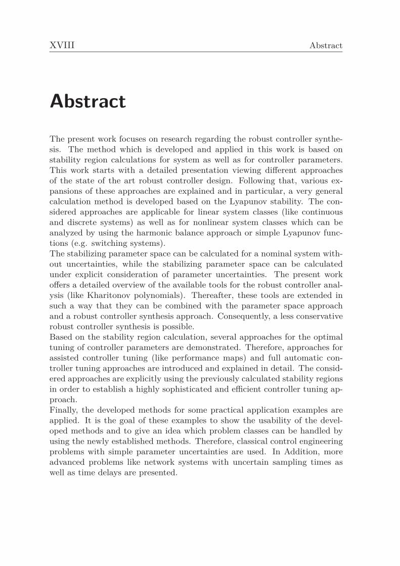
AbstractThe present work focuses on research regarding the robust controller synthe-sis. The method which is developed and applied in this work is based onstability region calculations for system as well as for controller parameters.This work starts with a detailed presentation viewing different approachesof the state of the art robust controller design. Following that, various ex-pansions of these approaches are explained and in particular, a very generalcalculation method is developed based on the Lyapunov stability. The con-sidered approaches are applicable for linear system classes (like continuousand discrete systems) as well as for nonlinear system classes which can beanalyzed by using the harmonic balance approach or simple Lyapunov func-tions (e.g. switching systems).The stabilizing parameter space can be calculated for a nominal system with-out uncertainties, while the stabilizing parameter space can be calculatedunder explicit consideration of parameter uncertainties. The present workoffers a detailed overview of the available tools for the robust controller anal-ysis (like Kharitonov polynomials). Thereafter, these tools are extended insuch a way that they can be combined with the parameter space approachand a robust controller synthesis approach. Consequently, a less conservativerobust controller synthesis is possible.Based on the stability region calculation, several approaches for the optimaltuning of controller parameters are demonstrated. Therefore, approaches forassisted controller tuning (like performance maps) and full automatic con-troller tuning approaches are introduced and explained in detail. The consid-ered approaches are explicitly using the previously calculated stability regionsin order to establish a highly sophisticated and efficient controller tuning ap-proach.Finally, the developed methods for some practical application examples areapplied. It is the goal of these examples to show the usability of the devel-oped methods and to give an idea which problem classes can be handled byusing the newly established methods. Therefore, classical control engineeringproblems with simple parameter uncertainties are used. In Addition, moreadvanced problems like network systems with uncertain sampling times aswell as time delays are presented.
Abstract XIX
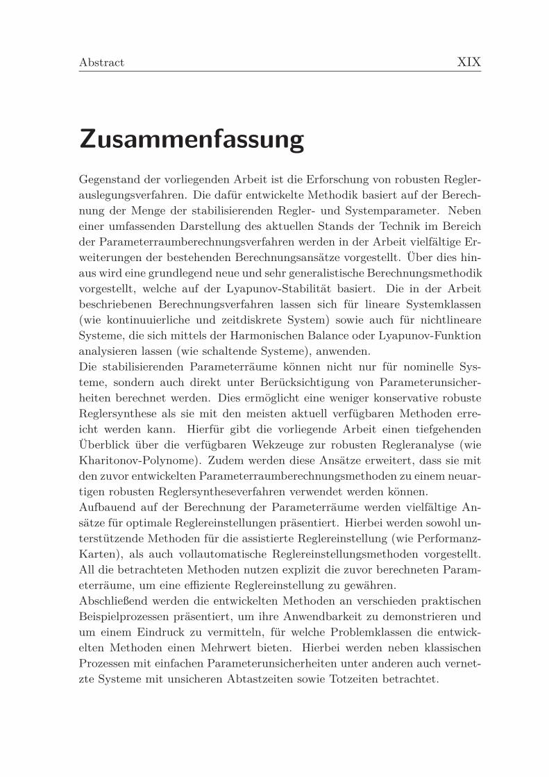
ZusammenfassungGegenstand der vorliegenden Arbeit ist die Erforschung von robusten Regler-auslegungsverfahren. Die dafür entwickelte Methodik basiert auf der Berech-nung der Menge der stabilisierenden Regler- und Systemparameter. Nebeneiner umfassenden Darstellung des aktuellen Stands der Technik im Bereichder Parameterraumberechnungsverfahren werden in der Arbeit vielfältige Er-weiterungen der bestehenden Berechnungsansätze vorgestellt. Über dies hin-aus wird eine grundlegend neue und sehr generalistische Berechnungsmethodikvorgestellt, welche auf der Lyapunov-Stabilität basiert. Die in der Arbeitbeschriebenen Berechnungsverfahren lassen sich für lineare Systemklassen(wie kontinuuierliche und zeitdiskrete System) sowie auch für nichtlineareSysteme, die sich mittels der Harmonischen Balance oder Lyapunov-Funktionanalysieren lassen (wie schaltende Systeme), anwenden.Die stabilisierenden Parameterräume können nicht nur für nominelle Sys-teme, sondern auch direkt unter Berücksichtigung von Parameterunsicher-heiten berechnet werden. Dies ermöglicht eine weniger konservative robusteReglersynthese als sie mit den meisten aktuell verfügbaren Methoden erre-icht werden kann. Hierfür gibt die vorliegende Arbeit einen tiefgehendenÜberblick über die verfügbaren Wekzeuge zur robusten Regleranalyse (wieKharitonov-Polynome). Zudem werden diese Ansätze erweitert, dass sie mitden zuvor entwickelten Parameterraumberechnungsmethoden zu einem neuar-tigen robusten Reglersyntheseverfahren verwendet werden können.Aufbauend auf der Berechnung der Parameterräume werden vielfältige An-sätze für optimale Reglereinstellungen präsentiert. Hierbei werden sowohl un-terstützende Methoden für die assistierte Reglereinstellung (wie Performanz-Karten), als auch vollautomatische Reglereinstellungsmethoden vorgestellt.All die betrachteten Methoden nutzen explizit die zuvor berechneten Param-eterräume, um eine effiziente Reglereinstellung zu gewähren.Abschließend werden die entwickelten Methoden an verschieden praktischenBeispielprozessen präsentiert, um ihre Anwendbarkeit zu demonstrieren undum einem Eindruck zu vermitteln, für welche Problemklassen die entwick-elten Methoden einen Mehrwert bieten. Hierbei werden neben klassischenProzessen mit einfachen Parameterunsicherheiten unter anderen auch vernet-zte Systeme mit unsicheren Abtastzeiten sowie Totzeiten betrachtet.

XX Abstract
1 Introduction 1
1 Introduction
Since 1600 BC or as far back as then at the least, the idea of feedbackcontrol was used for ship dynamic stabilization in Polynesia. Also note-worthy is the feedback mechanism in order to improve the accuracy ofwater clocks developed by Ktesibios in 285-222 BC. An additional con-siderable milestone was J. Watt’s centrifugal governor feedback controlsystem for steam engines. This was a key for the industrial revolu-tion. At the beginning of the 19th century common control engineeringand system theoretical basics were built up based on the work by J. C.Maxwell, I. Vyshnegradsky, E. J. Routh and A. Hurwitz. [22]Worldwide there were few universities offering classes in control engi-neering at the same time. Germany, for example, had a strong traditionin teaching control engineering and M. Tolle’s text book was alreadyavailable in 1905. His analysis was based on linearisation and examina-tion of the roots of the characteristic equation [314]. Since then, auto-matic control has emerged as a key enabler for many different modernengineering application systems of the 19th and 20th century. In themiddle of the 20th century the system theoretical research went througha renaissance based on the work of N. Wiener [336] who was stronglyinfluenced by the Russian neurophysiology scientists like P. K. Anochin[14]. This displays the fascinating interdisciplinary nature of this sci-entific discipline. The system theory is quite multidisciplinary, devel-oped mainly by engineers, mathematicians, economists and physicists.Today, control technology is found everywhere in daily life. Theoryand applications of control are growing rapidly in many different areas.Sometimes these developments are so fast paced that important linksbetween individual theoretical results are lost or not recognized.In this dissertation a variety of methods which were developed in theearly days of control engineering history are used and combined withlatest system theoretical results. The goal is to present ideas whichexpand the classical stability region calculation approaches with a newmethod for systematic controller synthesis and analysis with focus ontwo main challenges during the controller tuning: performance and ro-
2
bustness. Furthermore, the developed results will enrich the currentcontrol engineering education by demonstrating new relations betweenthe different classical system theoretical results in a new content.
Challenge one: Performance Let’s focus on the PID controller first.Developed in 1901 and commercially available since 1940, the PIDcontroller still is one of the most important controller types [13, 139].Around 95% of all controllers in process technology are PID controllers[18, 20, 143, 203, 339]. Also in the case of modern advanced controllers,the PID controller is often used as an underling stabilizing controller[20,87,347]. The reason for this is due to its simplicity and robustness.Even in the case of such simple controller types, a high percentage ofthese controllers is poorly tuned [97]. Studies like [48, 87] demonstratethat in practical applications, a poor controller tuning is found veryoften. A study of thousands of control loops in a few hundred processplants showed that 30% of the controllers are operating in the manualmode and another 30% are working worse than in manual mode basedwith regard to the poor controller tuning [97]. However, for simple LTIsystems a number of tuning rules exist which have been published since1942. Overviews of existing tuning methods can be found for examplein [20, 81, 308]. In [229], an impressive number of about 207 differenttuning rules is collected. A number of 143 new rules was published inthe period from 1993 to 2002. According to [297], the tuning of thethree PID parameters is not an easy task, nowadays. Hence, in the lastyears new PID tuning rules were published [122]. A major reason forpoor controller tuning is that common tuning methods are limited tovery restricted conditions in the plant, e.g. the concerned system orderor the pole and zero location [230]. General tuning methods for timedelay, unstable or non-minimum phase LTI systems of arbitrary orderwhich perform successfully independent of the design criteria do notexist [21,145,188].
Challenge two: Robustness At present, the most famous classicalcontroller tuning rule is the Ziegler-Nichols method [356]. Besides theadvantage of the simplicity of this tuning rule it also has some dis-advantages. The method is heuristically motivated and doesn’t con-sider model mismatches and uncertainties directly. Controller design
1 Introduction 3
approaches which take this into account are named robust control meth-ods. After the development of the negative feedback amplifier by H.Black in 1927, it took around 45 years until the term robust control ap-peared in literature. In 1945, a first robustness quantification methodwas introduced by H. W. Bode based on the phase margin and theamplitude margin. In the early days of robust control, there was a biggap between the mathematical control theory and the application whichlimited the dissemination of the developed methods. The military re-search in aviation was the first area in which robust control was applied.This lead to a push up effect regarding the development of robust con-trol design methods. At the beginning of 1970, the focus in the controlengineering community changed increasingly from optimal control torobust control. In 1968 I. Horowitz developed the first direct mathe-matical formulation of robust control. Since the early development ofrobust control, serious problems of optimal control were detected andafterwards robust control has been a central point in control engineering[263]. Accordingly, a variety of robust controller synthesis approachesexist today. The two most often used approaches are the frequency andthe parametric domain methods. The first one deals with frequencybased controller tuning methods like H∞ and μ synthesis [193]. Thesecond is based on the calculation of the space of all stabilizing con-troller parameters, mainly to handle parametric uncertainties. Today,general applicable robust design methods which are non-conservativeare still lacking [44, 142]. An inspiring survey of classical results andrecent developments in robust control is given in [244]. Currently, thefocus of the control engineering community goes back to optimal controldue to powerful optimal control concepts like model predictive controlwhich is inherently relatively robust [68].
Chosen method: Stability region calculation The original concept ofthe stability region calculation has a long history which can be tracedback to I. Vyshnegradsky [125, 326] who defined the stable region fora cubic polynomial in 1876. However, the first person who coined thename D-Decomposition for methods to calculate the stability region wasY. Neimark [218,219]. He proposed an algorithm for the calculation ofstable areas in the parameter space by the end of the 1940s. The algo-rithm is based on the computation of a particular decomposition of the
4
parameter space. In each region of the parameter space the number ofunstable characteristic roots is invariant with respect to all points of theparameter space inside the region. For each point on the boundaries thecorresponding characteristic equation has at least one root on the imag-inary axis. Inspired by the idea of Y. Neimark a lot of researchers haveexpanded on his ideas in various directions, like [4,44,124,286]. At theend of the last millennium several researchers were focused on findingall stabilizing controller parameters rather than finding an optimal setof controller parameters inside this region, like [27,149,292,301]. There-fore, a large number of calculation methods especially for the evaluationof the all stabilizing PID controller parameter space does exist. Despitethe fundamental importance of the stability region calculation most ofthe methods are rarely used in research and control engineering edu-cation today. Moreover, general applicable stability region calculationmethods are still being researched.
Proposed solution The structure of the present dissertation is as fol-lows. In section 2, a detailed analysis and comparison of the availablestability region calculation approaches will be presented. A systematicsummary of the stability region based controller tuning methods will beshown first. Furthermore, new interpretations and several expansionsto increase the applicability of the methods will be pointed out. In sec-tion 3 a less conservative integration of robustness requirements into thestability region calculation will be discussed. In this section new resultsregarding the less conservative direct consideration of the parameteruncertainties will be introduced. In section 4 an analysis and expansionof the stability region calculation methods for a performance require-ment based automatic controller tuning will be introduced. Finally insection 5, the implementation as well as the validation and the usabilityof the proposed methods will be discussed using practical applications.It is the final goal of this dissertation to increase the popularity of sta-bility region calculation techniques to a more frequently used methodfor controller synthesis and analysis. Therefore, the potential of themethod will be presented and critically discussed based on the under-ling theory as well as on different application examples. In addition,some further research topics will be outlined in order to show possiblefuture directions for this classical field of control engineering.
2 Stability region calculation 5
2 Stability region calculation
The basic requirement for controller design is asymptotic stability of theclosed-loop system. Therefore, it is intuitive to start with the controllertuning based on the stability region calculation. There are various ap-proaches in order to find the stabilizing regions in the space of thecontroller parameters. In the following a systematic summary and sev-eral expansions of the stability region-based controller tuning methodsare presented. For a detailed understanding of the problem, the rootlocus method is reviewed in the next section.
2.1 Root locus-based preliminaries
The root locus method was developed by W. Evans in 1948 [100, 101].It is a calculation approach for computing the closed-loop eigenvaluesas a function of the open-loop gain. It offers a possibility to studythe stability as well as the performance of a system. Today, it is aclassical tool for system synthesis and analysis of LTI systems [277].However, time delay systems are disregarded [91, 191, 231] or directlyexcluded [348] from the root locus study. Accordingly, the followingsection focuses on the root locus method for LTI time delay systems.In practice, time delay systems are often used to model the behavior ofsystems in the field of biology, chemistry, economics, physics, populationdynamic and engineering science [254, 293, 294]. The first analyses oftime delay systems were performed by the Bernoulli brothers and L.Euler in the 18th century [109]. With the systematic studies by A.Myshkis and R. Bellman, a deeper understanding of these systems began[109] and since 1960 many publications have been produced in this fieldof study [128]. The topic of robust control for time delay systems led tothe time delay boom of the middle 1990s [109]. Since then the numberof publications regarding time delay systems has been growing fromyear to year [229].
6 2.1 Root locus-based preliminaries
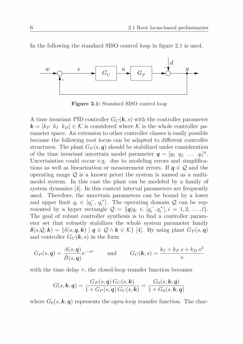
In the following the standard SISO control loop in figure 2.1 is used.
Figure 2.1: Standard SISO control loop
A time invariant PID controller GC(k, s) with the controller parameterk = [kP kI kD] ∈ K is considered where K is the whole controller pa-rameter space. An extension to other controller classes is easily possiblebecause the following root locus can be adapted to different controllerstructures. The plant GP (s, q) should be stabilized under considerationof the time invariant uncertain model parameter q = [q1 q2 . . . ql]ᵀ.Uncertainties could occur e.g. due to modeling errors and simplifica-tions as well as linearization or measurement errors. If q ∈ Q and theoperating range Q is a known priori the system is named as a multi-model system. In this case the plant can be modeled by a family ofsystem dynamics [4]. In this context interval parameters are frequentlyused. Therefore, the uncertain parameters can be bound by a lowerand upper limit qi ∈ [q−
i , q+i ]. The operating domain Q can be rep-
resented by a hyper rectangle Q = {q|qi ∈ [q−i , q+
i ], i = 1, 2, . . . , l}.The goal of robust controller synthesis is to find a controller param-eter set that robustly stabilizes the whole system parameter familyδ(s,Q, k) = {δ(s, q, k) | q ∈ Q ∧ k ∈ K} [4]. By using plant GP (s, q)and controller GC(k, s) in the form
GP (s, q) =A(s, q)B(s, q)
e−sτ and GC(k, s) =kI + kP s + kD s2
s
with the time delay τ , the closed-loop transfer function becomes
G(s, k, q) =GP (s, q) GC(s, k)
1 + GP (s, q) GC(s, k)=
G0(s, k, q)1 + G0(s, k, q)
where G0(s, k, q) represents the open-loop transfer function. The char-
2 Stability region calculation 7
acteristic polynomial can be calculated by computing the poles of theclosed-loop transfer function. It is given by
δ(s, kI , kP , kD, q) = A(s, q) (kI + kP s + kD s2) + s B(s, q) esτ .
with A(s, q) = a0 + a1 s + . . . + am sm am �= 0,
and B(s, q) = b0 + b1 s + . . . + bn sn = s B(s, q), bn �= 0, (2.1)
n→ Degree of B(s, q) = Degree of B(s, q) + 1,
m→ Degree of A(s, q).
Analytical root locus description 1 The open-loop gain k(k, q) shallbe the only varying parameter in this section. The location of the zerossi of δ(s, k, q) is a function of the open-loop gain k(k, q). The family ofall zeros si for a given interval of the open-loop gain k(k, q) is namedthe root locus. For k(k, q) > 0 it is the primary and for k(k, q) < 0 thecomplementary root locus. Starting point for the root locus calculationis the modified characteristic equation
A(s, q)(kI + kP s + kD s2)B(s, q∗) s esτ
= k(k, q)A(s, k∗, q∗)B(s, q∗) esτ
= −1
with fixed parameters denoted by ∗. After substituting s = σ + jω,the equation can be split into a magnitude and a phase equation. Itholds for the magnitude |e−(σ+jω) τ | = |e−σ τ e−jω τ | = e−σ τ because|e jω τ | = | cos ωτ − j sin ωτ | = 1. Therefore the magnitude condition isresulting:
|k(k, q∗)| = 1e−σ τ
|B(s, q∗)||A(s, k∗, q∗)|
(2.2)
The magnitude condition is used to parametrize the root locus curvewith the varying parameter k(k, q∗). The phase condition is
∠(k, q) + ∠A(s, k∗, q∗) − ∠B(s, q∗) + ∠e−sτ = ∠ (−1) . (2.3)
1A first implementation and discussion of the proposed ideas has been presented in[S02, S29]. The following section is based on this. The key ideas of this sectionwere published during the DFG project AB 65/2-3 in [271,273].
8 2.1 Root locus-based preliminaries
Based on the relation ∠e−τ s = ∠e−σ τ + ∠e−jω τ = 0◦ + ∠(cos(ω τ)−j sin(ω τ)) = −ω τ a positive feedback k(kP ,q) > 0 is the result:
∠A(s, k∗, q∗) − ∠B(s, q∗) = n 180◦ + ω τ with n = ±1,±3,±5, . . .
A negative feedback k(kP ,q) > 0 results in:
∠A(s, k∗, q∗) − ∠B(s, q∗) = n 360◦ + ω τ with n = 0,±1,±2,±3, . . .
The phase condition is used to find the points in the complex domainwhich belong to the root locus. W. J. Palm [239] developed construc-tion rules for the root locus for time delay systems, similar to the wellknown delay-free case. Unfortunately, the construction rules becomevery complex in the delay case. In order to construct root locus di-agrams accurate analytical approaches are developed. Therefore thecharacteristic polynomial is reformulated in a form that the resultingequation maps the root locus with algebraic equations. In 1966, V.Krishnan developed a semi-analytical approach for low order delay-freesystems [184] based on the idea of K. Steiglitz [302]. This approachwas first implemented as a computer-aided program by Z. Klagsbrunn[176] in 1968 and was later extended to delay systems by K. S. Yeung[345] in 1982. Parallel to this C. Chang developed an analytical methodwhich considers delay systems in 1965 [70]. He used the fact that aclosed-loop pole does exist when the real and the imaginary part of thecharacteristic polynomial are equal to zero. Based on this he stated theroot locus equation as a function of the real (�) and imaginary (�) partof the polynomial:
�A(s, k, q)�B(s, q) − �B(s, q)�A(s, k, q) = 0 (2.4)
Unfortunately the evaluating effort is growing disproportionately forhigh order systems. The analogy to the potential field theory offersa better understanding of the analytical root locus equations whichwas first presented by W. Evens [100]. By using the analogy to theelectrostatic field, G. Grübel and L. Schmieder presented generalizedproperties of root loci in 1967 [123]. T. Becker used the idea of potentialflows to study delay systems in 1988 [38]. An illustrative study for delay-free systems was presented by P. Tsiotras in 2005. He used a 3D bodeplot to show the analogy between poles and springs in mountains aswell as zeros and sinks. The root loci represent rivers [315].
2 Stability region calculation 9
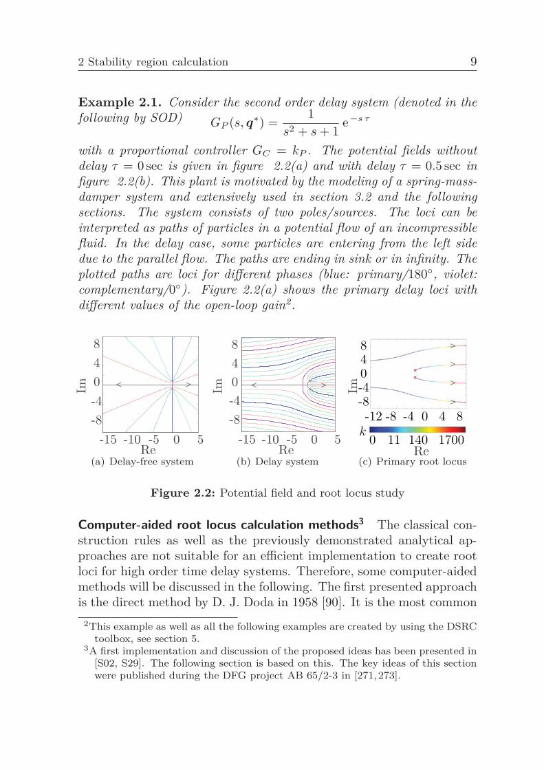
Example 2.1. Consider the second order delay system (denoted in thefollowing by SOD) GP (s, q∗) =
1s2 + s + 1
e−s τ
with a proportional controller GC = kP . The potential fields withoutdelay τ = 0 sec is given in figure 2.2(a) and with delay τ = 0.5 sec infigure 2.2(b). This plant is motivated by the modeling of a spring-mass-damper system and extensively used in section 3.2 and the followingsections. The system consists of two poles/sources. The loci can beinterpreted as paths of particles in a potential flow of an incompressiblefluid. In the delay case, some particles are entering from the left sidedue to the parallel flow. The paths are ending in sink or in infinity. Theplotted paths are loci for different phases (blue: primary/180◦, violet:complementary/0◦). Figure 2.2(a) shows the primary delay loci withdifferent values of the open-loop gain2.
-15 -10 -5 0 5-8-4048
Re
Im < >
(a) Delay-free system
-15 -10 -5 0 5-8-4048
Re
Im < >
(b) Delay system
-12 -8 -4 0 4 8-8-4048
0 11 140 1700Re
Im>
>
>
>
k
(c) Primary root locus
Figure 2.2: Potential field and root locus study
Computer-aided root locus calculation methods3 The classical con-struction rules as well as the previously demonstrated analytical ap-proaches are not suitable for an efficient implementation to create rootloci for high order time delay systems. Therefore, some computer-aidedmethods will be discussed in the following. The first presented approachis the direct method by D. J. Doda in 1958 [90]. It is the most common
2This example as well as all the following examples are created by using the DSRCtoolbox, see section 5.
3A first implementation and discussion of the proposed ideas has been presented in[S02, S29]. The following section is based on this. The key ideas of this sectionwere published during the DFG project AB 65/2-3 in [271,273].
10 2.1 Root locus-based preliminaries
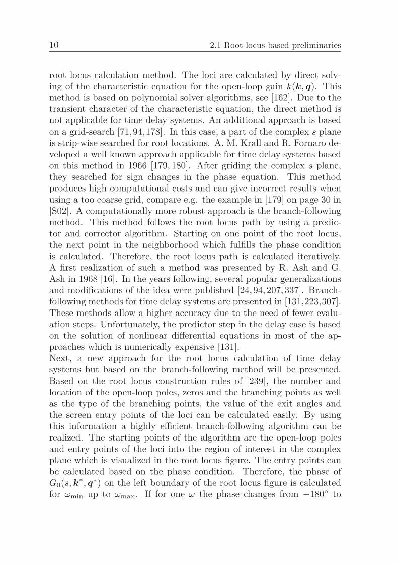
root locus calculation method. The loci are calculated by direct solv-ing of the characteristic equation for the open-loop gain k(k, q). Thismethod is based on polynomial solver algorithms, see [162]. Due to thetransient character of the characteristic equation, the direct method isnot applicable for time delay systems. An additional approach is basedon a grid-search [71,94,178]. In this case, a part of the complex s planeis strip-wise searched for root locations. A. M. Krall and R. Fornaro de-veloped a well known approach applicable for time delay systems basedon this method in 1966 [179, 180]. After griding the complex s plane,they searched for sign changes in the phase equation. This methodproduces high computational costs and can give incorrect results whenusing a too coarse grid, compare e.g. the example in [179] on page 30 in[S02]. A computationally more robust approach is the branch-followingmethod. This method follows the root locus path by using a predic-tor and corrector algorithm. Starting on one point of the root locus,the next point in the neighborhood which fulfills the phase conditionis calculated. Therefore, the root locus path is calculated iteratively.A first realization of such a method was presented by R. Ash and G.Ash in 1968 [16]. In the years following, several popular generalizationsand modifications of the idea were published [24, 94, 207, 337]. Branch-following methods for time delay systems are presented in [131,223,307].These methods allow a higher accuracy due to the need of fewer evalu-ation steps. Unfortunately, the predictor step in the delay case is basedon the solution of nonlinear differential equations in most of the ap-proaches which is numerically expensive [131].Next, a new approach for the root locus calculation of time delaysystems but based on the branch-following method will be presented.Based on the root locus construction rules of [239], the number andlocation of the open-loop poles, zeros and the branching points as wellas the type of the branching points, the value of the exit angles andthe screen entry points of the loci can be calculated easily. By usingthis information a highly efficient branch-following algorithm can berealized. The starting points of the algorithm are the open-loop polesand entry points of the loci into the region of interest in the complexplane which is visualized in the root locus figure. The entry points canbe calculated based on the phase condition. Therefore, the phase ofG0(s, k∗, q∗) on the left boundary of the root locus figure is calculatedfor ωmin up to ωmax. If for one ω the phase changes from −180◦ to
2 Stability region calculation 11
Figure 2.3: Root locus searching algorithm
180◦, a primary root locus enters the figure at this position. Figure2.3 illustrates the procedure of the branch-following method. Duringthe procedure, the angle criterion is evaluated for all candidate pointssk+1(j) of the searching area. At each starting point, the neighboringpoint is searched which satisfies the angle criterion best (e.g. sk+1(2)in figure 2.3). The searching grid can be adapted dynamically untila desired accuracy in the evaluation of the angle criterion is achieved.After the best candidate point sk+1 in the searching area is found, thispoint will be set as a start point for the next searching area and thesearching algorithm continues iteratively. The orientation of the search-ing area depends on the pole exit angle. In case of branching points,the searching area is deflected into a new direction depending on thetype of branching point (e.g. by 90◦ in the case of a double branchingpoint, see figure 2.3). For more information about the handling of highorder branching points, see [94,240]. When the locus has reached a zeroor the edge of the screen, the algorithm ends. The branch-followingalgorithm of all loci can be performed in parallel to reduce calculationtime. The values of the controller gain can be calculated by using themagnitude criterion and be plotted in form of contour maps, similar to[32]. This algorithm is used in the present dissertation to produce allthe depicted root loci.
4A first implementation and discussion of the proposed ideas has been presentedin [S02, S29]. The following section is based on this.
12 2.1 Root locus-based preliminaries
Results of the system approximation4 Time delay systems can be ap-proximated by systems which only consist of the two rightmost eigen-values of the delay system. There is a rule of thumb which states: ifa pole of a system without zeros has a three times smaller distance tothe imaginary axis than the other poles this dominant pole will mainlyinfluence the system behavior [276]. Some more advanced model reduc-tion techniques of time delay systems are discussed e.g. in [192,255,335].In general the differences between delay and delay-free systems regard-ing the settling time as well as the natural frequency become larger forincreasing values of τ . Therefore, the quality of the approximation be-comes worse for increasing delays.This can be explained by the study of R. Bellman and K. L. Cooke [39].They stated that the roots for systems with increasing delays are tend-ing to ±∞ fast. This can also be seen by using the phase condition inequation (2.3). After checking the phase condition along the imaginaryaxis, the intersection points of the root locus and the imaginary axiscan be calculated. It turns out that the distance of poles in real direc-tions is increasing for increasing delays. Moreover, based on the phasecondition it can be seen that an increasing τ leads to a decreasing ω forthe nth intersection point. Consequently, for an increasing τ the poledistance in the imaginary direction decreases. Based on the previouslystated rule of thumb, it is obvious that for increasing delays the notconsidered effect of high order poles leads to a decreasing quality of thesystem approximation.The problem of the fragility of the system approximation can be solvedby using approximations with higher order rational fractional functionslike in the Taylor approximation. In 1979 some fundamental problemsregarding the Taylor approximation of time delay systems were alreadyshown [138,199]. One problem is that the Taylor approximation of timedelay systems with an Taylor polynomial of an order equal and biggersix may lead to unstable systems [138]. Today, the most popular delayapproximation method is the Padé approximation developed by H. Padéin 1892. By using this technique the time delay system is approximatedby a finite number of pairs of poles and zeros. This method is unre-stricted concerning the system order. However, numerical problems canoccur by high dimensional Padé approximations (in Matlab greater orequal order of ten). In the following example, the effect of increasingdelays and system approximations will be illustrated.
2 Stability region calculation 13
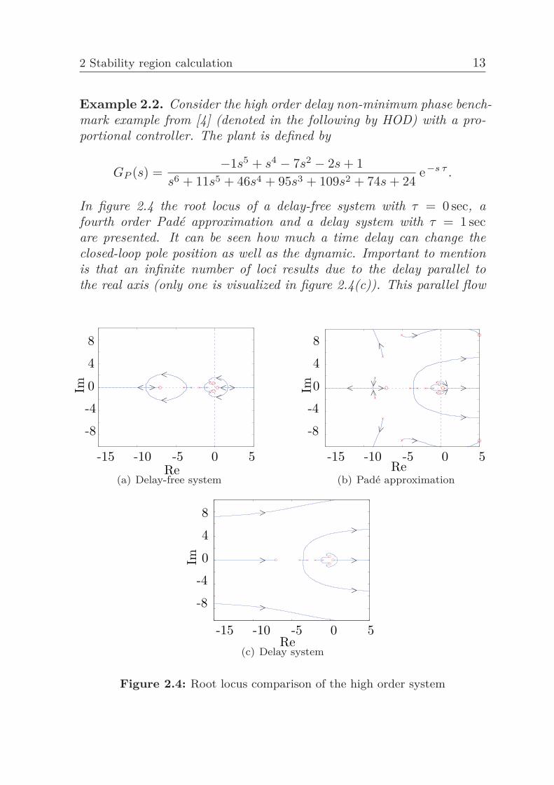
Example 2.2. Consider the high order delay non-minimum phase bench-mark example from [4] (denoted in the following by HOD) with a pro-portional controller. The plant is defined by
GP (s) =−1s5 + s4 − 7s2 − 2s + 1
s6 + 11s5 + 46s4 + 95s3 + 109s2 + 74s + 24e−s τ .
In figure 2.4 the root locus of a delay-free system with τ = 0 sec, afourth order Padé approximation and a delay system with τ = 1 secare presented. It can be seen how much a time delay can change theclosed-loop pole position as well as the dynamic. Important to mentionis that an infinite number of loci results due to the delay parallel tothe real axis (only one is visualized in figure 2.4(c)). This parallel flow
-15 -10 -5 0 5
-8
-4
0
4
8
Im
Re(a) Delay-free system
-15 -10 -5 0 5
-8
-4
0
4
8
Im
Re(b) Padé approximation
-15 -10 -5 0 5
-8
-4
0
4
8
Im
Re(c) Delay system
Figure 2.4: Root locus comparison of the high order system
14 2.1 Root locus-based preliminaries
(a) Pole location (b) Step response
Figure 2.5: Effect of varying delay values for the SOD system
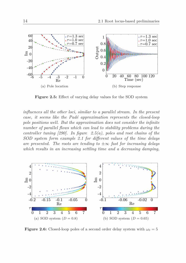
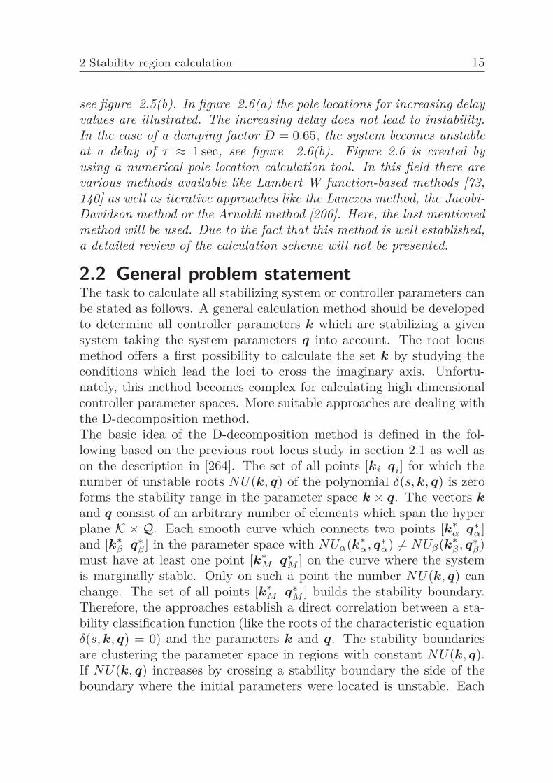
influences all the other loci, similar to a parallel stream. In the presentcase, it seems like the Padé approximation represents the closed-looppole positions well. But the approximation does not consider the infinitenumber of parallel flows which can lead to stability problems during thecontroller tuning [290]. In figure 2.5(a), poles and root chains of theSOD system form example 2.1 for different values of the time delaysare presented. The roots are tending to ±∞ fast for increasing delayswhich results in an increasing settling time and a decreasing damping,
(a) SOD system (D = 0.8) (b) SOD system (D = 0.65)
Figure 2.6: Closed-loop poles of a second order delay system with ω0 = 5
2 Stability region calculation 15
see figure 2.5(b). In figure 2.6(a) the pole locations for increasing delayvalues are illustrated. The increasing delay does not lead to instability.In the case of a damping factor D = 0.65, the system becomes unstableat a delay of τ ≈ 1 sec, see figure 2.6(b). Figure 2.6 is created byusing a numerical pole location calculation tool. In this field there arevarious methods available like Lambert W function-based methods [73,140] as well as iterative approaches like the Lanczos method, the Jacobi-Davidson method or the Arnoldi method [206]. Here, the last mentionedmethod will be used. Due to the fact that this method is well established,a detailed review of the calculation scheme will not be presented.
2.2 General problem statementThe task to calculate all stabilizing system or controller parameters canbe stated as follows. A general calculation method should be developedto determine all controller parameters k which are stabilizing a givensystem taking the system parameters q into account. The root locusmethod offers a first possibility to calculate the set k by studying theconditions which lead the loci to cross the imaginary axis. Unfortu-nately, this method becomes complex for calculating high dimensionalcontroller parameter spaces. More suitable approaches are dealing withthe D-decomposition method.The basic idea of the D-decomposition method is defined in the fol-lowing based on the previous root locus study in section 2.1 as well ason the description in [264]. The set of all points [ki qi] for which thenumber of unstable roots NU(k, q) of the polynomial δ(s, k, q) is zeroforms the stability range in the parameter space k × q. The vectors kand q consist of an arbitrary number of elements which span the hyperplane K × Q. Each smooth curve which connects two points [k∗
α q∗α]
and [k∗β q∗
β ] in the parameter space with NUα(k∗α, q∗
α) �= NUβ(k∗β , q∗
β)must have at least one point [k∗
M q∗M ] on the curve where the system
is marginally stable. Only on such a point the number NU(k, q) canchange. The set of all points [k∗
M q∗M ] builds the stability boundary.
Therefore, the approaches establish a direct correlation between a sta-bility classification function (like the roots of the characteristic equationδ(s, k, q) = 0) and the parameters k and q. The stability boundariesare clustering the parameter space in regions with constant NU(k, q).If NU(k, q) increases by crossing a stability boundary the side of theboundary where the initial parameters were located is unstable. Each
16 2.2 General problem statement
(a) Finite crossing (b) Infinite crossing
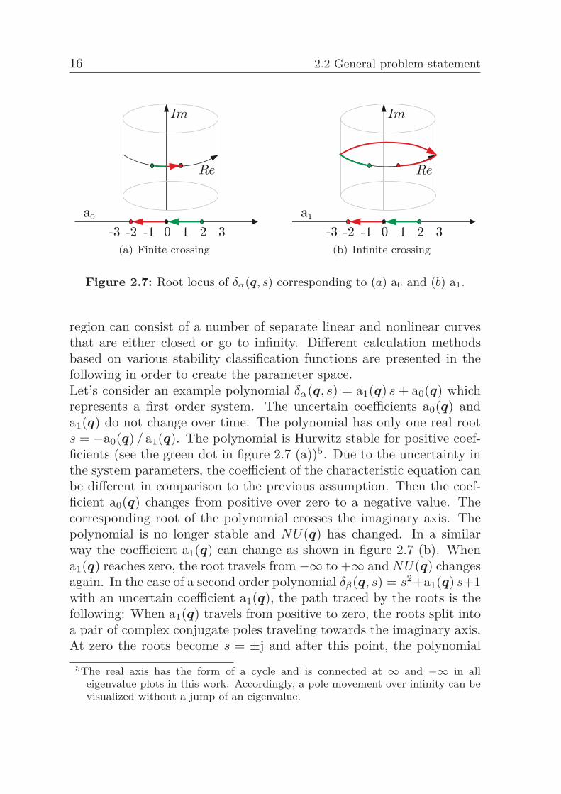
Figure 2.7: Root locus of δα(q, s) corresponding to (a) a0 and (b) a1.
region can consist of a number of separate linear and nonlinear curvesthat are either closed or go to infinity. Different calculation methodsbased on various stability classification functions are presented in thefollowing in order to create the parameter space.Let’s consider an example polynomial δα(q, s) = a1(q) s + a0(q) whichrepresents a first order system. The uncertain coefficients a0(q) anda1(q) do not change over time. The polynomial has only one real roots = −a0(q) / a1(q). The polynomial is Hurwitz stable for positive coef-ficients (see the green dot in figure 2.7 (a))5. Due to the uncertainty inthe system parameters, the coefficient of the characteristic equation canbe different in comparison to the previous assumption. Then the coef-ficient a0(q) changes from positive over zero to a negative value. Thecorresponding root of the polynomial crosses the imaginary axis. Thepolynomial is no longer stable and NU(q) has changed. In a similarway the coefficient a1(q) can change as shown in figure 2.7 (b). Whena1(q) reaches zero, the root travels from −∞ to +∞ and NU(q) changesagain. In the case of a second order polynomial δβ(q, s) = s2+a1(q) s+1with an uncertain coefficient a1(q), the path traced by the roots is thefollowing: When a1(q) travels from positive to zero, the roots split intoa pair of complex conjugate poles traveling towards the imaginary axis.At zero the roots become s = ±j and after this point, the polynomial
5The real axis has the form of a cycle and is connected at ∞ and −∞ in alleigenvalue plots in this work. Accordingly, a pole movement over infinity can bevisualized without a jump of an eigenvalue.
2 Stability region calculation 17
loses its stability and NU(q) changes. In general the roots of a systemmove along a continuous curve caused by a continuous change of thecoefficients of the characteristic polynomial. This shows (based on thecontinuous pole movement) that a polynomial becomes unstable whenthe roots are crossing the imaginary axis or infinity. In the following,the stability boundaries can be created directly by calculating only thecoefficients of the polynomial for which such a change in NU(q) occurs.This is much more efficient in comparison to a brute force search ofstabilizing parameter combinations inside the parameter space becausein this case problems, like those mentioned in section 2.1 regarding theroot locus grid-search, could occur.
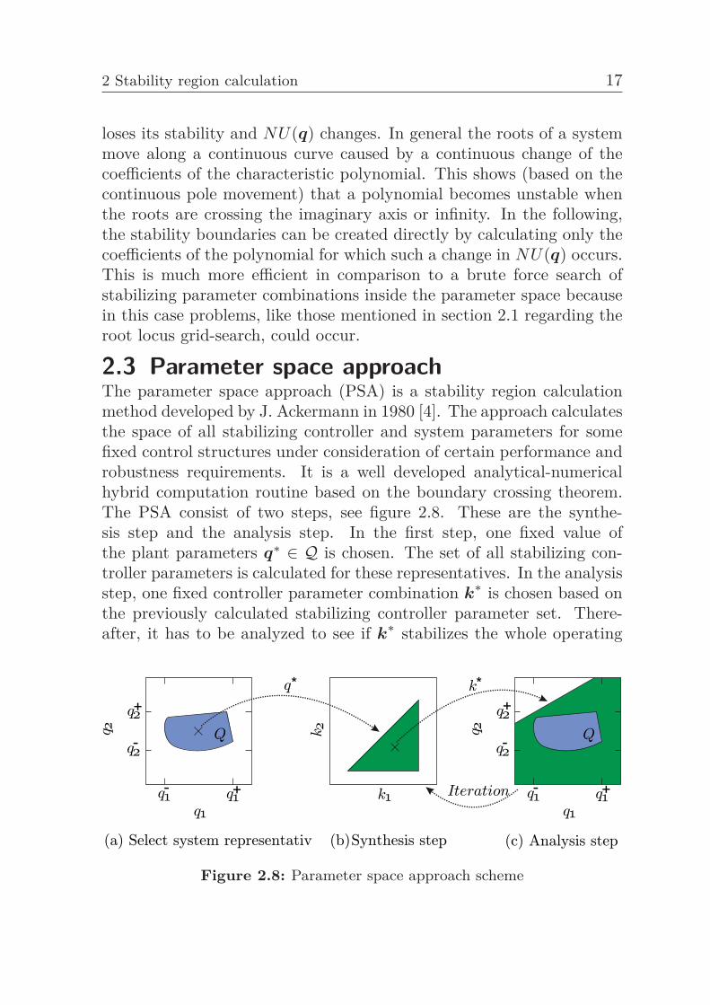
2.3 Parameter space approachThe parameter space approach (PSA) is a stability region calculationmethod developed by J. Ackermann in 1980 [4]. The approach calculatesthe space of all stabilizing controller and system parameters for somefixed control structures under consideration of certain performance androbustness requirements. It is a well developed analytical-numericalhybrid computation routine based on the boundary crossing theorem.The PSA consist of two steps, see figure 2.8. These are the synthe-sis step and the analysis step. In the first step, one fixed value ofthe plant parameters q∗ ∈ Q is chosen. The set of all stabilizing con-troller parameters is calculated for these representatives. In the analysisstep, one fixed controller parameter combination k∗ is chosen based onthe previously calculated stabilizing controller parameter set. There-after, it has to be analyzed to see if k∗ stabilizes the whole operating
Figure 2.8: Parameter space approach scheme
18 2.3 Parameter space approach
domain Q. The classical approach uses the characteristic polynomialδ(s, k, q) = 0 from equation (2.1) as stability decision function. Accord-ingly, the boundary crossing theorem stated that a polynomial familyδ(s, k∗,Q) = {δ(s, k∗, q)|q ∈ Q} is robust stable if:
1. a stable polynomial δ(s, k∗, q) ∈ δ(s, k∗,Q) exists and2. jω /∈ roots
[δ(s, k∗,Q)
],∀ ω ≥ 0.
Based on this and similar to the previous section, three cases of imagi-nary axis boundary crossings are studied:
1. Real root boundary (RRB)A root of the polynomial crosses the imaginary axis on the real axisthrough the origin. The stability changes at δ(s = 0, k, q) = 0.
2. Complex root boundary (CRB)A root of the polynomial crosses the imaginary axis with complexconjugated pole pairs. The stability changes at δ(s = jω,k,q) = 0.
3. Infinite root boundary (IRB)A root of the polynomial leaves the right or left half plane atinfinity. The stability changes at δ(|s| → ∞, k, q) = 0.
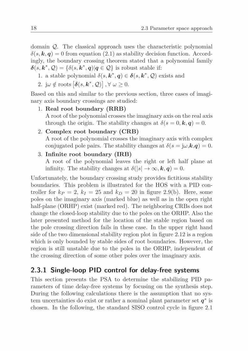
Unfortunately, the boundary crossing study provides fictitious stabilityboundaries. This problem is illustrated for the HOS with a PID con-troller for kP = 2, kI = 25 and kD = 20 in figure 2.9(b). Here, somepoles on the imaginary axis (marked blue) as well as in the open righthalf-plane (ORHP) exist (marked red). The neighboring CRBs does notchange the closed-loop stability due to the poles on the ORHP. Also thelater presented method for the location of the stable region based onthe pole crossing direction fails in these case. In the upper right handside of the two dimensional stability region plot in figure 2.12 is a regionwhich is only bounded by stable sides of root boundaries. However, theregion is still unstable due to the poles in the ORHP, independent ofthe crossing direction of some other poles over the imaginary axis.
2.3.1 Single-loop PID control for delay-free systemsThis section presents the PSA to determine the stabilizing PID pa-rameters of time delay-free systems by focusing on the synthesis step.During the following calculations there is the assumption that no sys-tem uncertainties do exist or rather a nominal plant parameter set q∗ ischosen. In the following, the standard SISO control cycle in figure 2.1
2 Stability region calculation 19
with τ = 0 sec is used. Based on the characteristic equation (2.1) thecalculation rules for the three stability boundary types are presented.
Real root boundary6
In the case of a RRB the roots cross the imaginary axis at the origin.Therefore, substituting s = 0 in the characteristic polynomial gives:δ(s = 0, kI , kP , kD, q∗) = 0 ⇒ A(s = 0, q∗) kI + B(s = 0, q∗) = 0
⇒ a0 kI + (b0 = 0) = 0 ⇒ kI = 0
Differentiating systems which have a polynomial A(s, q∗) with a0 = 0are building a special case which is not studied in the classical literature.In such a case a single s can be factorized and eliminated from thecharacteristic equation δ(s = 0, kI , kP , kD, q∗) = 0 ⇒ a1 kI + b1 =0 ⇒ kI = b1/a1. Based on the previous equation sets the RRB is:
kI =
{− b0
a0= 0
a0= 0, if a0 �= 0
− b1a1
, if a0 = 0(2.5)
Consider a system of the form A(s) = a1 s + a0 and B(s) = b1 s + b0.The closed-loop poles can be calculated as
s1 = −b0/(a1kD s2 + (b2 + a1kP )s + b1 + a1 kI)
s2,3 = − b2 + a1 kP
2 a1 kD︸ ︷︷ ︸γ
±
√(b2 + a1 kP
2 a1 kD
)2−(
b1 + a1 kI
a1 kD
).
Due to the integrative part of the controller (b0 = 0) s1 = 0 holds,independent of the controller gains, see figure 2.9 (a). The other twopoles s2,3 are sensitive to the controller gains. These roots are followingan asymptote parallel to the imaginary axis by varying kI . The distancebetween the asymptote and the imaginary axis is γ/2. After a certainvalue of kI , the poles s1,2 reach the real axis and are deflected by 90 ◦.Next, at the stability-critical value of kI (see RRB), one pole crossesthe imaginary axis.
6A first implementation and discussion of the proposed ideas has been presentedin [S30]. The following section is based on this.
20 2.3 Parameter space approach
(a) Example of RRB pole movement (b) Stab. uncritical pole distribution
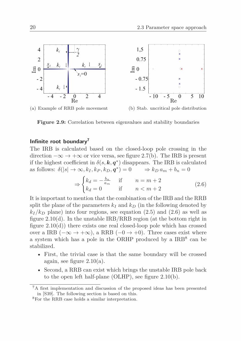
Figure 2.9: Correlation between eigenvalues and stability boundaries
Infinite root boundary7
The IRB is calculated based on the closed-loop pole crossing in thedirection −∞→ +∞ or vice versa, see figure 2.7(b). The IRB is presentif the highest coefficient in δ(s, k, q∗) disappears. The IRB is calculatedas follows: δ(|s| → ∞, kI , kP , kD, q∗) = 0 ⇒ kD am + bn = 0
⇒{
kd = − bn
amif n = m + 2
kd = 0 if n < m + 2(2.6)
It is important to mention that the combination of the IRB and the RRBsplit the plane of the parameters kI and kD (in the following denoted bykI/kD plane) into four regions, see equation (2.5) and (2.6) as well asfigure 2.10(d). In the unstable IRB/RRB region (at the bottom right infigure 2.10(d)) there exists one real closed-loop pole which has crossedover a IRB (−∞→ +∞), a RRB (−0→ +0). Three cases exist wherea system which has a pole in the ORHP produced by a IRB8 can bestabilized.
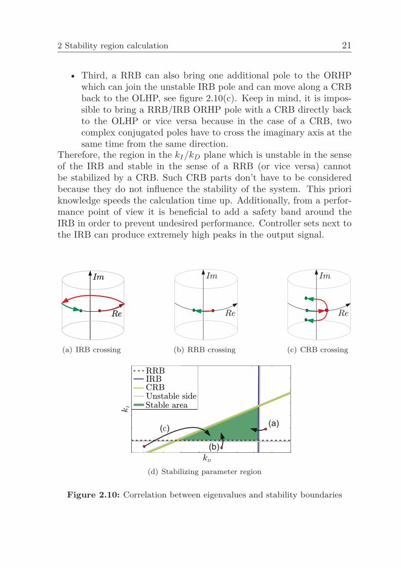
• First, the trivial case is that the same boundary will be crossedagain, see figure 2.10(a).
• Second, a RRB can exist which brings the unstable IRB pole backto the open left half-plane (OLHP), see figure 2.10(b).
7A first implementation and discussion of the proposed ideas has been presentedin [S39]. The following section is based on this.
8For the RRB case holds a similar interpretation.
2 Stability region calculation 21
• Third, a RRB can also bring one additional pole to the ORHPwhich can join the unstable IRB pole and can move along a CRBback to the OLHP, see figure 2.10(c). Keep in mind, it is impos-sible to bring a RRB/IRB ORHP pole with a CRB directly backto the OLHP or vice versa because in the case of a CRB, twocomplex conjugated poles have to cross the imaginary axis at thesame time from the same direction.
Therefore, the region in the kI/kD plane which is unstable in the senseof the IRB and stable in the sense of a RRB (or vice versa) cannotbe stabilized by a CRB. Such CRB parts don’t have to be consideredbecause they do not influence the stability of the system. This prioriknowledge speeds the calculation time up. Additionally, from a perfor-mance point of view it is beneficial to add a safety band around theIRB in order to prevent undesired performance. Controller sets next tothe IRB can produce extremely high peaks in the output signal.
(a) IRB crossing (b) RRB crossing (c) CRB crossing
(d) Stabilizing parameter region
Figure 2.10: Correlation between eigenvalues and stability boundaries
22 2.3 Parameter space approach
Complex root boundary9
Based on the substitution δ(s = jω, k, q∗) = 0 the CRBs can be calcu-lated. The resulting equation is now depending on ω and k. Hence, itis not easily possible to extract the stability boundary equations as inthe two previous cases. In the following, a calculation scheme is pre-sented to get stability boundary equations only as a function of k. Thefirst step is to split the characteristic equation δ(jω, k, q∗) into its realpart �δ(ω, k, q∗) and imaginary part �δ(ω, k, q∗) which is similar tothe proposed idea has been equation (2.4):
δ(jω, k, q∗) = �δ(ω, k, q∗) + j�δ(ω, k, q∗)
with
A(jω, q∗) =�A(ω, q∗) + j�A(ω, q∗), B(jω, q∗) = �B(ω, q∗) + j�B(ω, q∗).
This can be reformulated in the following equation set:(�δ(ω, k,q∗)�δ(ω, k,q∗)
)=(�A − ω2�A
�A − ω2�A
)(kI
kD
)+(�B − kP ω�A
�B + kP ω�A
)= 0
Next, the short notation with scripted arguments �A|B|δ = �A|B|δ(ω, q∗)and �A|B|δ = �A|B|δ(ω, q∗) is used for the real and imaginary part of thepolynomial A(jω, q) and B(jω, q). Then, the substitution z = kI−kD ω2
in the equation for the imaginary part of the char. equation �δ gives:
�δ = �B + ω kP �A + �A (kI − kD ω2)︸ ︷︷ ︸z
= 0⇒ z = −�B + ω kP �A
�A
Applying the same substitution to �δ results in:
�δ = �B − ω kP �A + �A (kI − kD ω2)︸ ︷︷ ︸z
= 0
⇒�δ = �B − ωkP�A + �A
(−�B + ωkP�A
�A
)= 0
9A first implementation and discussion of the proposed ideas has been presentedin [S28, S30, S31, S39]. The following section is based on this.
2 Stability region calculation 23
Solving this equation for kP gives
kP (ω, q∗) =�B(ω, q∗)�A(ω, q∗)−�A(ω, q∗)�B(ω, q∗)
ω(�2A(ω, q∗) + �2
A(ω, q∗)). (2.7)
Every value pair which fulfills equation (2.7) is denoted as (k∗p, ωS,t)
with t = 1, 2, .... The variable ωS,t represents the crossing frequency.Similar to the root locus study this frequency corresponds to the inter-section point of the closed-loop pole and the imaginary axis. Substitut-ing equation (2.7) into �δ or �δ gives:
�δ =�B + ωS,t�A
(�B �A −�A �B
ωS,t (�2A + �2
A)
)︸ ︷︷ ︸
k∗P
−kD ω2S,t�A + kI �A = 0 or
�δ =�B − ωS,t�A
(�B �A −�A �B
ωS,t (�2A + �2
A)
)︸ ︷︷ ︸
k∗P
−kD ω2S,t�A + kI�A = 0
These equations can be solved for kI and results in
kI(ωS,t, k∗P , kD, kI , q∗) = ωS,t
2kD + k0I,�|�(ωS,t, k∗
P ) with (2.8)
k0I,�(ωS,t, k∗
P , q∗) =
(−ωS,t k∗
P �A(ωS,t)−�B(ωS,t)�A(ωS,t)
)or
k0I,�(ωS,t, k∗
P , q∗) =
(ωS,t k∗
P �A(ωS,t)−�B(ωS,t)�A(ωS,t)
),
where k0I,�(ωS,t, k∗
P , q∗) belongs to �δ(ω, k, q∗) and k0I,�(ωS,t, k∗
P , q∗)to �δ(ω, k, q∗). Both equations are similar. Only for the special case�A(ω, q∗) = 0 or �A(ω, q∗) = 0, the k0
I,�|�(ωS,t, k∗P , q∗) equation has to
be chosen carefully to prevent the denominator going to zero. Based onthis calculation, the CRB calculation scheme works as follows. First,a fixed value k∗
P has to be substituted in equation (2.7). Thereafter,this equation can be solved for ωS,t because this equation is no longera function of kI or kD. The solutions are named singular frequencies.In a second step, ωS,t can be substituted into equation (2.8). After
24 2.3 Parameter space approach
the substitution, this equation is a linear affine equation in kI/kD. Foreach singular frequency, one CRB results. The singular frequencies canbe interpreted as the slope and the intersection points of the resultinglinear stability boundaries in the kI/kD plane. It is obvious that theslope of the CRBs must be positive, see equation (2.8).RRB and CRBs can be summarized as finite root boundaries (FRB).Theoretically, the RBB is already included in the CRB case with ωS = 0.However, it makes sense to study it separately due to the different cal-culation scheme.
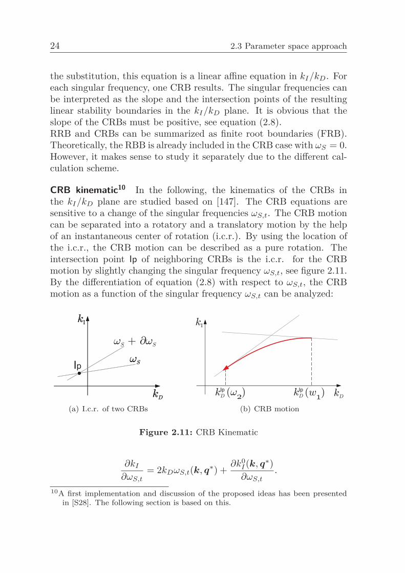
CRB kinematic10 In the following, the kinematics of the CRBs inthe kI/kD plane are studied based on [147]. The CRB equations aresensitive to a change of the singular frequencies ωS,t. The CRB motioncan be separated into a rotatory and a translatory motion by the helpof an instantaneous center of rotation (i.c.r.). By using the location ofthe i.c.r., the CRB motion can be described as a pure rotation. Theintersection point Ip of neighboring CRBs is the i.c.r. for the CRBmotion by slightly changing the singular frequency ωS,t, see figure 2.11.By the differentiation of equation (2.8) with respect to ωS,t, the CRBmotion as a function of the singular frequency ωS,t can be analyzed:
(a) I.c.r. of two CRBs (b) CRB motion
Figure 2.11: CRB Kinematic
∂kI
∂ωS,t= 2kDωS,t(k, q∗) +
∂k0I (k, q∗)∂ωS,t
.
10A first implementation and discussion of the proposed ideas has been presentedin [S28]. The following section is based on this.
2 Stability region calculation 25
Next, only the rotatory motion is studied ∂kI/∂ωS,t = 0. Based on thetwo previously mentioned equations, the coordinates of the i.c.r. canbe expressed as a curve in the kI/kD plane parametrized by ωS,t:(
kIpD(ωS,t)
kIpI (ωS,t)
)=
⎛⎝ − ∂k0I
∂ωS,t
12ωS,t
− ∂k0I
∂ωS,t
ωS,t
2 + k0I
⎞⎠ , ωS,t ∈ [ω−S,t, ω+
S,t] (2.9)
The slope of the tangent on this curve is:
∂kIpI
∂kIpD
=∂kIp
I /∂ωS,t
∂kIpD/∂ωS,t
=
−∂2k0
I
∂ω2S,t
−∂k0
I
2∂ωS,t+
∂k0I
∂ωS,t
−∂2k0
I
∂ω2S,t
12ωS,t
+∂k0
I
∂ωS,t
12ω2
S,t
= ω2S,t
−∂2k0
I
∂ω2S,t
ωS,t
2+
∂k0I
2∂ωS,t
−∂2k0
I
∂ω2S,t
ωS,t
2+
∂k0I
2∂ωS,t
The slope results to ω2S,t due to the fact that the last term of the product
in the previous equation is equal to one. The i.c.r. trajectory representsthe curve which describes the CRB movement as a function of the sin-gular frequency ωS,t, see figure 2.11. The i.c.r tends to the left side forincreasing values of ωS,t and has a turning point on each local extremumof kIp
D, see [147].
Calculation of stable kP interval11 For each fixed k∗P a set of CRBs
results. Accordingly, there is a need to find a finite stabilizing kP inter-val. An intuitive method for this is based on the following equations
kP = �B �A − �A �B
ω(�2A + �2
A)=
ω �B �A − ω �A �B
ω(�2A + �2
A)=
�B �A − �A �B
|A|2
=�B �A − �A �B
|A||A| = 〈A, B〉|A||A|
|B||B|
= 〈A, B〉|A||B|
|B||A| = 〈A, B〉
|A||B||GP |−1
= − cos∠(A, B) |GP (ω, q∗)|−1.
Consequently, a bound for the absolute value of kP can be calculated.The stabilizing kp interval depends only on the plant GP (ω, q∗):
kP (ω, q∗) ≤ |GP (ω, q∗)|−1 ≤ supω∈R+ |GP (ω, q∗)|−1
11A first implementation and discussion of the proposed ideas have been presentedin [S30, S31]. The following section is based on this.
26 2.3 Parameter space approach
No stability-critical boundary can be found outside this bound. ForkP values outside this bound, there isn’t any controller parameter setexisting which causes a stability change (imaginary axis crossing) of theclosed-loop system. Compared to the following advanced kP -intervalstudy, this bound is quite imprecise but much more intuitive. Assumethat A(s) has no zeros on the imaginary axis. Based on [29,147,301] thestability condition for a kp can be expressed by the minimum numberof singular frequencies
zmin ≥⌊
n′ −m + 2p− 12
⌋, (2.10)
where n′ = max(n,m+2) is the degree of the characteristic polynomial,p is the number of zeros of A(s) in the right half plane and �.� denotesthe floor function. The proof and the extension in the case of A(s)where the zeros are located on the imaginary axis, is given in [29]. Byanalyzing equation (2.7) it is obvious that a different number of singularfrequencies results for different values of kp.
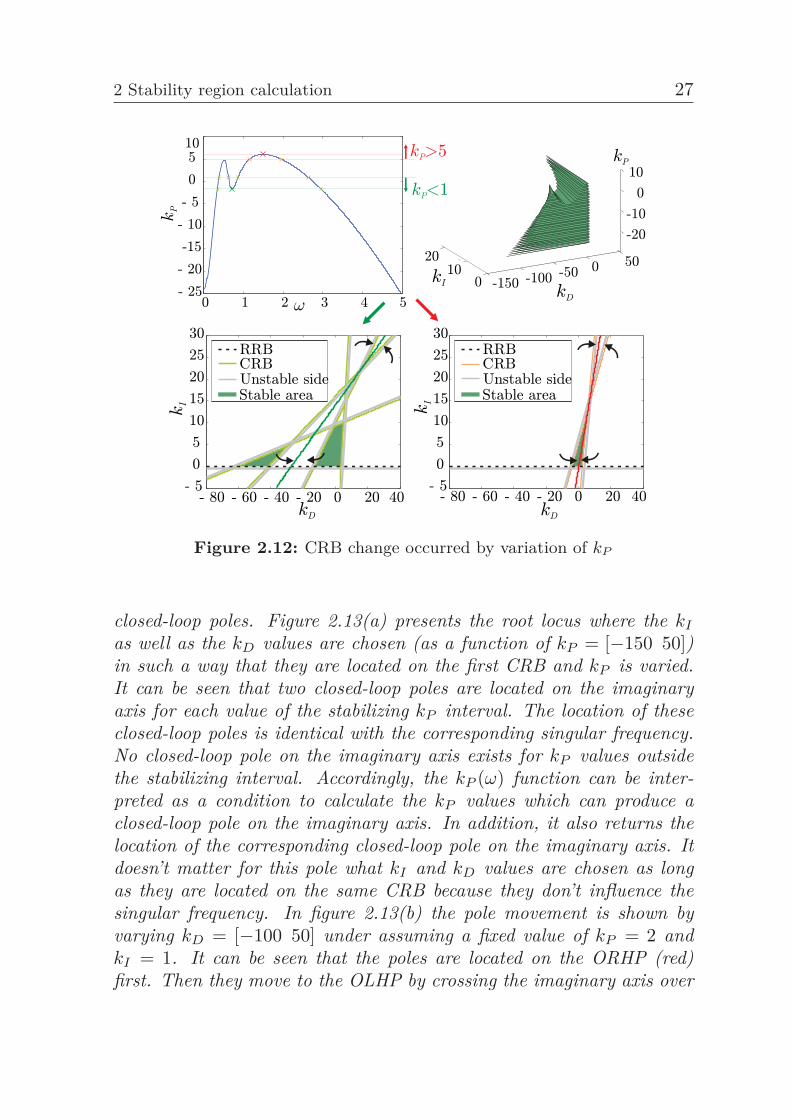
Example 2.3. Consider the delay-free version of the high order non-minimum phase benchmark example from [4], introduced in example2.2. This system is often used in the parameter space community be-cause of the nicely shaped stability domain. The plant is defined byA(s) = −1s5 + s4 − 7s2 − 2s + 1 and B(s) = s6 + 11s5 + 46s4 +95s3 + 109s2 + 74s + 24. By analyzing figure 2.12 it is obvious that thenumber of ωS,t changes at the extrema of kP in equation (2.7). Aftercalculating the extrema of kP , possible kP intervals result. After eval-uating the condition in equation (2.10), the stable kP interval resultsdirectly. The kP limits can also be easily explained by using the doubleroot boundaries. These are two CRBs which result from two singularfrequencies which converge to one by varying the kP value. The singu-lar frequencies are the intersection points of the kP (ω) function (blue)and the freely selectable kP value (e.g. red and green line) in figure2.12. As presented in figure 2.12 these boundaries can cut off the un-stable as well as the stable parameter region easily. This effect is thereason why such a double root boundary influences the stabilizing kP
range. Something similar happens at a triple point: Two CRBs inter-sect with an other root boundary in one point. This effect shrinks thestabilizing kP interval, studiedin detail in [147]. This context can beintuitively explained by studying the movement of the location of the
2 Stability region calculation 27
Figure 2.12: CRB change occurred by variation of kP
closed-loop poles. Figure 2.13(a) presents the root locus where the kI
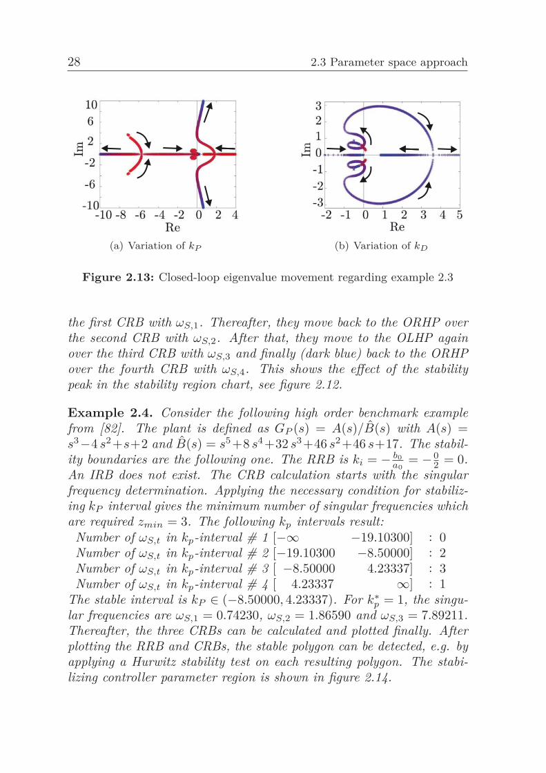
as well as the kD values are chosen (as a function of kP = [−150 50])in such a way that they are located on the first CRB and kP is varied.It can be seen that two closed-loop poles are located on the imaginaryaxis for each value of the stabilizing kP interval. The location of theseclosed-loop poles is identical with the corresponding singular frequency.No closed-loop pole on the imaginary axis exists for kP values outsidethe stabilizing interval. Accordingly, the kP (ω) function can be inter-preted as a condition to calculate the kP values which can produce aclosed-loop pole on the imaginary axis. In addition, it also returns thelocation of the corresponding closed-loop pole on the imaginary axis. Itdoesn’t matter for this pole what kI and kD values are chosen as longas they are located on the same CRB because they don’t influence thesingular frequency. In figure 2.13(b) the pole movement is shown byvarying kD = [−100 50] under assuming a fixed value of kP = 2 andkI = 1. It can be seen that the poles are located on the ORHP (red)first. Then they move to the OLHP by crossing the imaginary axis over
28 2.3 Parameter space approach
(a) Variation of kP (b) Variation of kD
Figure 2.13: Closed-loop eigenvalue movement regarding example 2.3
the first CRB with ωS,1. Thereafter, they move back to the ORHP overthe second CRB with ωS,2. After that, they move to the OLHP againover the third CRB with ωS,3 and finally (dark blue) back to the ORHPover the fourth CRB with ωS,4. This shows the effect of the stabilitypeak in the stability region chart, see figure 2.12.
Example 2.4. Consider the following high order benchmark examplefrom [82]. The plant is defined as GP (s) = A(s)/B(s) with A(s) =s3−4 s2+s+2 and B(s) = s5+8 s4+32 s3+46 s2+46 s+17. The stabil-ity boundaries are the following one. The RRB is ki = − b0
a0= − 0
2 = 0.An IRB does not exist. The CRB calculation starts with the singularfrequency determination. Applying the necessary condition for stabiliz-ing kP interval gives the minimum number of singular frequencies whichare required zmin = 3. The following kp intervals result:
Number of ωS,t in kp-interval # 1 [−∞ −19.10300] : 0Number of ωS,t in kp-interval # 2 [−19.10300 −8.50000] : 2Number of ωS,t in kp-interval # 3 [ −8.50000 4.23337] : 3Number of ωS,t in kp-interval # 4 [ 4.23337 ∞] : 1
The stable interval is kP ∈ (−8.50000, 4.23337). For k∗p = 1, the singu-
lar frequencies are ωS,1 = 0.74230, ωS,2 = 1.86590 and ωS,3 = 7.89211.Thereafter, the three CRBs can be calculated and plotted finally. Afterplotting the RRB and CRBs, the stable polygon can be detected, e.g. byapplying a Hurwitz stability test on each resulting polygon. The stabi-lizing controller parameter region is shown in figure 2.14.
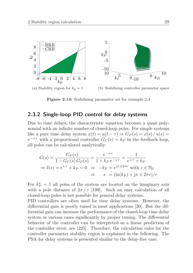
2 Stability region calculation 29
(a) Stability region for kp = 1
-100 10
0510-10
-5
0
5
kDkI
kP
(b) Stabilizing controller parameter space
Figure 2.14: Stabilizing parameter set for example 2.4
2.3.2 Single-loop PID control for delay systemsDue to time delays, the characteristic equation becomes a quasi poly-nomial with an infinite number of closed-loop poles. For simple systemslike a pure time delay system x(t) = u(t− τ)⇒ GP (s) = x(s) / u(s) =e−s τ with a proportional controller GC(s) = kP in the feedback loop,all poles can be calculated analytically:
G(s) =GP (s)
1−GC(s) GP (s)=
e−s τ
1 + kP e−s τ=
1es τ + kP
⇒ δ(s) = es τ + kP = 0 ⇒ −kP = e jπ±2πr with r ∈ N0
⇒ s = (ln(kP ) + jπ ± 2πr)/τ
For k∗P = 1 all poles of the system are located on the imaginary axis
with a pole distance of 2π / τ [199]. Such an easy calculation of allclosed-loop poles is not possible for general delay systems.PID controllers are often used for time delay systems. However, thedifferential gain is poorly tuned in most applications [20]. But the dif-ferential gain can increase the performance of the closed-loop time delaysystem in various cases significantly by proper tuning. The differentialbehavior of the controller can be interpreted as a linear prediction ofthe controller error, see [225]. Therefore, the calculation rules for thecontroller parameter stability region is explained in the following. ThePSA for delay systems is presented similar to the delay-free case.
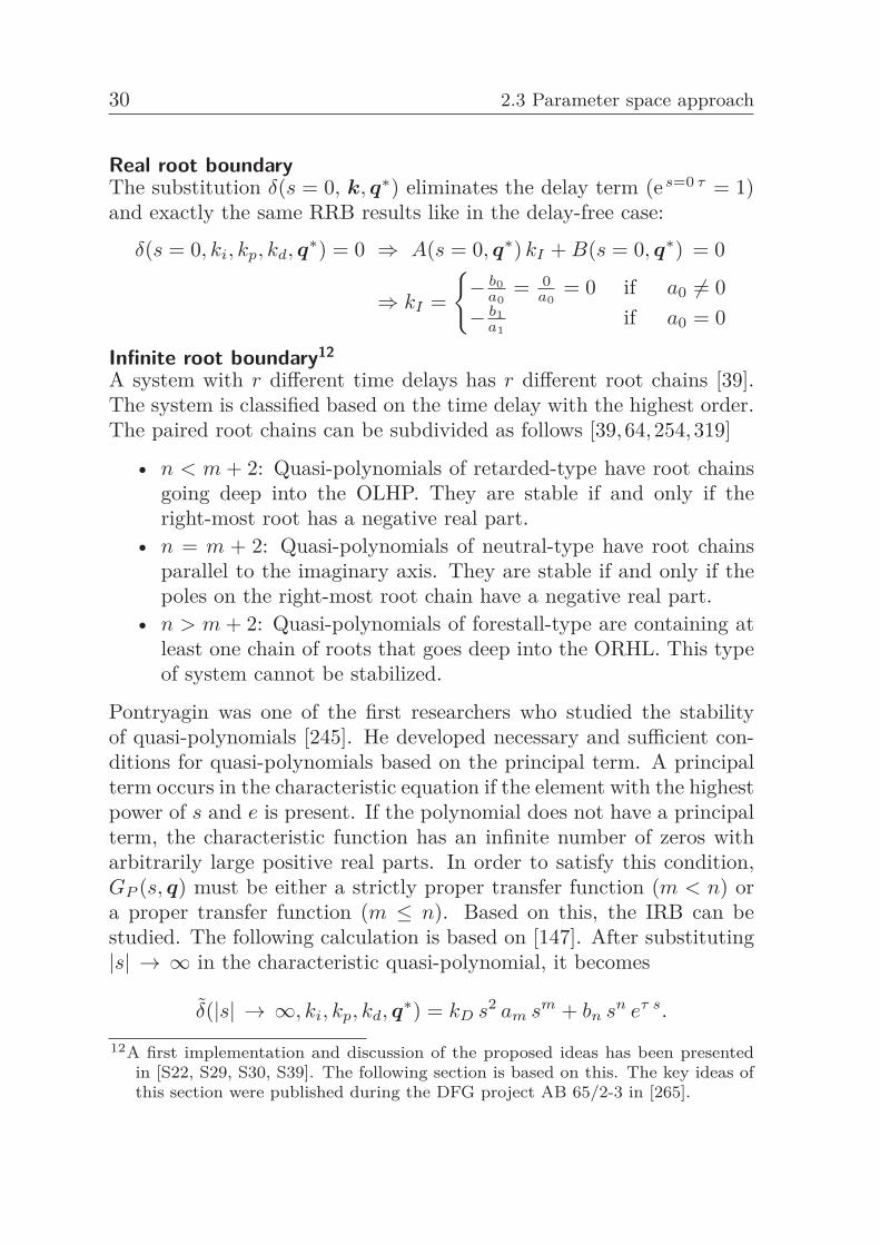
30 2.3 Parameter space approach
Real root boundaryThe substitution δ(s = 0, k, q∗) eliminates the delay term (es=0 τ = 1)and exactly the same RRB results like in the delay-free case:
δ(s = 0, ki, kp, kd, q∗) = 0 ⇒ A(s = 0, q∗) kI + B(s = 0, q∗) = 0
⇒ kI =
{− b0
a0= 0
a0= 0 if a0 �= 0
− b1a1
if a0 = 0
Infinite root boundary12
A system with r different time delays has r different root chains [39].The system is classified based on the time delay with the highest order.The paired root chains can be subdivided as follows [39,64,254,319]
• n < m + 2: Quasi-polynomials of retarded-type have root chainsgoing deep into the OLHP. They are stable if and only if theright-most root has a negative real part.
• n = m + 2: Quasi-polynomials of neutral-type have root chainsparallel to the imaginary axis. They are stable if and only if thepoles on the right-most root chain have a negative real part.
• n > m + 2: Quasi-polynomials of forestall-type are containing atleast one chain of roots that goes deep into the ORHL. This typeof system cannot be stabilized.
Pontryagin was one of the first researchers who studied the stabilityof quasi-polynomials [245]. He developed necessary and sufficient con-ditions for quasi-polynomials based on the principal term. A principalterm occurs in the characteristic equation if the element with the highestpower of s and e is present. If the polynomial does not have a principalterm, the characteristic function has an infinite number of zeros witharbitrarily large positive real parts. In order to satisfy this condition,GP (s, q) must be either a strictly proper transfer function (m < n) ora proper transfer function (m ≤ n). Based on this, the IRB can bestudied. The following calculation is based on [147]. After substituting|s| → ∞ in the characteristic quasi-polynomial, it becomes
δ(|s| → ∞, ki, kp, kd, q∗) = kD s2 am sm + bn sn eτ s.
12A first implementation and discussion of the proposed ideas has been presentedin [S22, S29, S30, S39]. The following section is based on this. The key ideas ofthis section were published during the DFG project AB 65/2-3 in [265].

2 Stability region calculation 31
For the root calculation, δ(|s| → ∞, ki, kp, kd, q∗) has to be zero. More-over, the exponential term is eliminated by the logarithm function:
0 =1τ
ln
(kD s2 am sm
−bn sn
)− s
If n = m + 2 holds, the quasi-polynomial δ has the root
s∞ =1τ
ln(−kD am
bn
)with �s∞ =
1τ
ln
(∣∣∣∣kD am
bn
∣∣∣∣)
,
�s∞ =
{(2 k+1)π
τ , for kD am bn >02 k π
τ , for kD am bn <0and k ∈ Z.
In the neutral case, the roots are located on a line parallel to the imag-inary axis. An IRB exists, if this line lies on the imaginary axis, like inthe example at the beginning of section 2.3.2. Therefore, it must hold�s∞ = 0⇒ dn = bn. Hence, the IRB results in two stability boundariesin the controller parameter space:
kD = ±bn/am, if n = m + 2 (2.11)This is the same result as in the principal term study of Pontryaginpresented previously. For the retarded case, it holds:
kD = 0, if n < m (2.12)The retarded case can be interpreted similarly to the delay-free IRB. Inthis case, one pole goes to the ORHP over infinity caused by the IRB.Only a RRB can stabilize such a system. An infinite number of polescrosses the stability boundary at the same time in the neutral case.Therefore, a system becomes an infinite number of ORHP poles. Thesepoles cannot be moved back to the OLHP by any combination of RRBand CRBs. Based on this phenomenon, the IRB can be interpreted asa global stability boundary in the neutral case. All RRB and CRBs onthe unstable side of the IRB do not have to be checked because all theseboundaries are fictitious stability boundaries.
Complex root boundary13
The CRB can be calculated by using the substitution s = jω in the
13A first implementation and discussion of the proposed ideas has been presentedin [S30, S31, S39]. The following section is based on this.
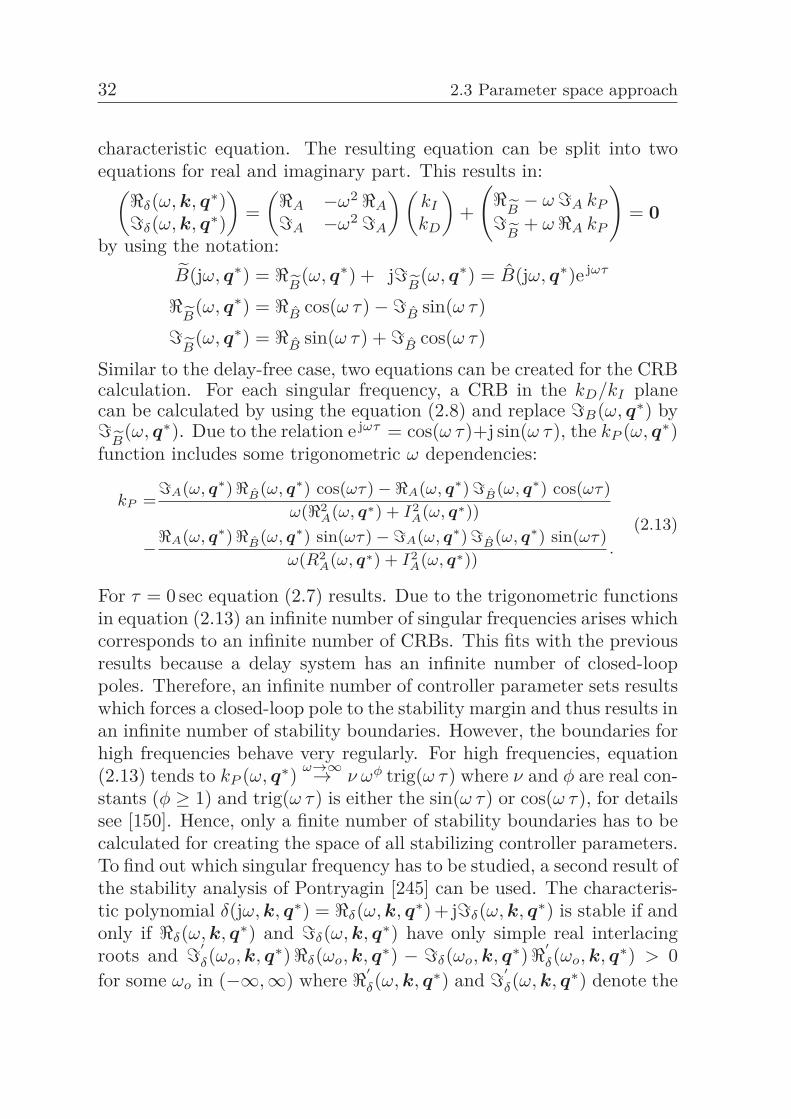
32 2.3 Parameter space approach
characteristic equation. The resulting equation can be split into twoequations for real and imaginary part. This results in:(�δ(ω, k, q∗)�δ(ω, k, q∗)
)=(�A −ω2 �A
�A −ω2 �A
)(kI
kD
)+
(�
B− ω�A kP
�B
+ ω�A kP
)= 0
by using the notation:B(jω, q∗) = �
B(ω, q∗) + j�
B(ω, q∗) = B(jω, q∗)e jωτ
�B
(ω, q∗) = �B cos(ω τ)−�B sin(ω τ)
�B
(ω, q∗) = �B sin(ω τ) + �B cos(ω τ)
Similar to the delay-free case, two equations can be created for the CRBcalculation. For each singular frequency, a CRB in the kD/kI planecan be calculated by using the equation (2.8) and replace �B(ω, q∗) by�
B(ω, q∗). Due to the relation e jωτ = cos(ω τ)+j sin(ω τ), the kP (ω, q∗)
function includes some trigonometric ω dependencies:
kP =�A(ω, q∗) �B(ω, q∗) cos(ωτ) − �A(ω, q∗) �B(ω, q∗) cos(ωτ)
ω(�2A(ω, q∗) + I2
A(ω, q∗))
−�A(ω, q∗) �B(ω, q∗) sin(ωτ) − �A(ω, q∗) �B(ω, q∗) sin(ωτ)ω(R2
A(ω, q∗) + I2A(ω, q∗))
.
(2.13)
For τ = 0 sec equation (2.7) results. Due to the trigonometric functionsin equation (2.13) an infinite number of singular frequencies arises whichcorresponds to an infinite number of CRBs. This fits with the previousresults because a delay system has an infinite number of closed-looppoles. Therefore, an infinite number of controller parameter sets resultswhich forces a closed-loop pole to the stability margin and thus results inan infinite number of stability boundaries. However, the boundaries forhigh frequencies behave very regularly. For high frequencies, equation(2.13) tends to kP (ω, q∗) ω→∞→ ν ωφ trig(ω τ) where ν and φ are real con-stants (φ ≥ 1) and trig(ω τ) is either the sin(ω τ) or cos(ω τ), for detailssee [150]. Hence, only a finite number of stability boundaries has to becalculated for creating the space of all stabilizing controller parameters.To find out which singular frequency has to be studied, a second result ofthe stability analysis of Pontryagin [245] can be used. The characteris-tic polynomial δ(jω, k, q∗) = �δ(ω, k, q∗) + j�δ(ω, k, q∗) is stable if andonly if �δ(ω, k, q∗) and �δ(ω, k, q∗) have only simple real interlacingroots and �′
δ(ωo, k, q∗)�δ(ωo, k, q∗) − �δ(ωo, k, q∗)�′δ(ωo, k, q∗) > 0
for some ωo in (−∞,∞) where �′δ(ω, k, q∗) and �′
δ(ω, k, q∗) denote the
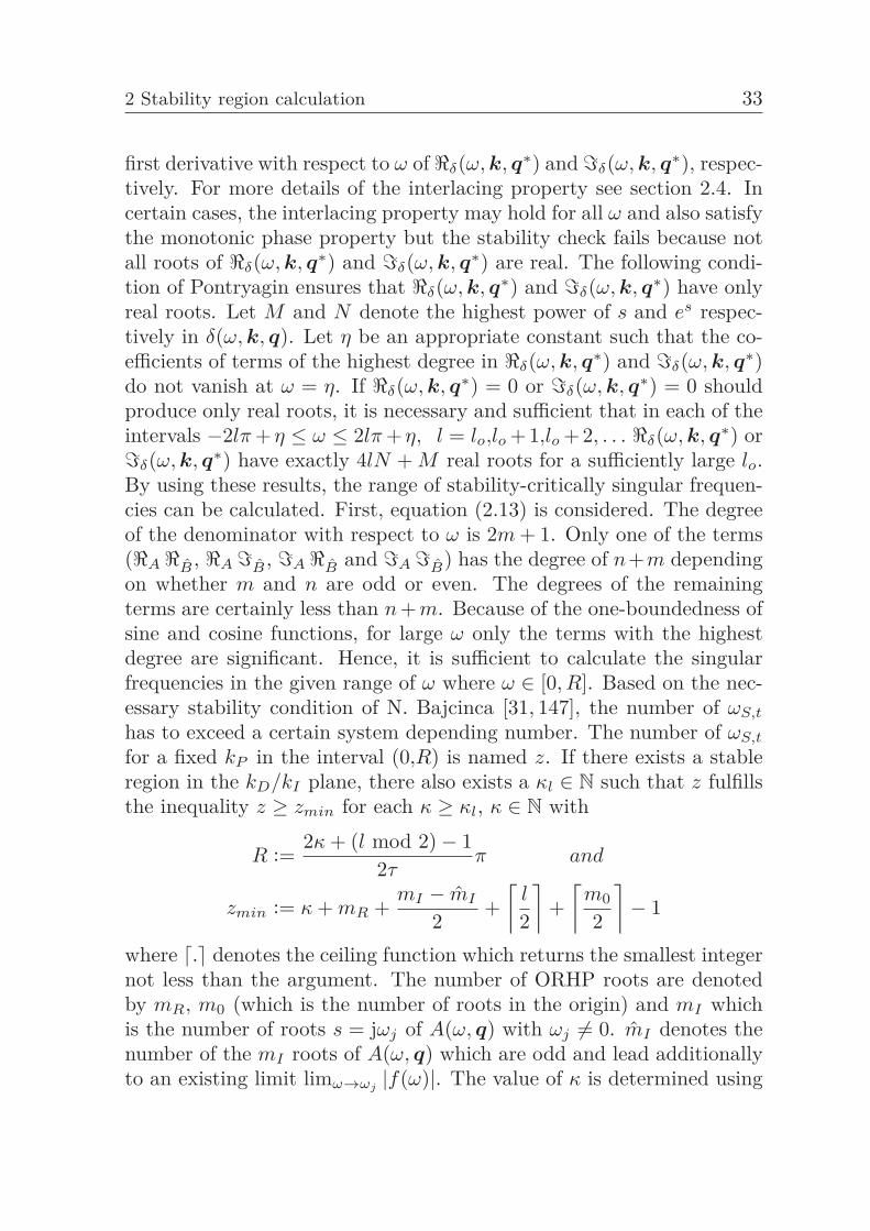
2 Stability region calculation 33
first derivative with respect to ω of �δ(ω, k, q∗) and �δ(ω, k, q∗), respec-tively. For more details of the interlacing property see section 2.4. Incertain cases, the interlacing property may hold for all ω and also satisfythe monotonic phase property but the stability check fails because notall roots of �δ(ω, k, q∗) and �δ(ω, k, q∗) are real. The following condi-tion of Pontryagin ensures that �δ(ω, k, q∗) and �δ(ω, k, q∗) have onlyreal roots. Let M and N denote the highest power of s and es respec-tively in δ(ω, k, q). Let η be an appropriate constant such that the co-efficients of terms of the highest degree in �δ(ω, k, q∗) and �δ(ω, k, q∗)do not vanish at ω = η. If �δ(ω, k, q∗) = 0 or �δ(ω, k, q∗) = 0 shouldproduce only real roots, it is necessary and sufficient that in each of theintervals −2lπ + η ≤ ω ≤ 2lπ + η, l = lo,lo + 1,lo + 2, . . . �δ(ω, k, q∗) or�δ(ω, k, q∗) have exactly 4lN + M real roots for a sufficiently large lo.By using these results, the range of stability-critically singular frequen-cies can be calculated. First, equation (2.13) is considered. The degreeof the denominator with respect to ω is 2m + 1. Only one of the terms(�A �B , �A �B , �A �B and �A �B) has the degree of n+m dependingon whether m and n are odd or even. The degrees of the remainingterms are certainly less than n + m. Because of the one-boundedness ofsine and cosine functions, for large ω only the terms with the highestdegree are significant. Hence, it is sufficient to calculate the singularfrequencies in the given range of ω where ω ∈ [0, R]. Based on the nec-essary stability condition of N. Bajcinca [31, 147], the number of ωS,t
has to exceed a certain system depending number. The number of ωS,t
for a fixed kP in the interval (0,R) is named z. If there exists a stableregion in the kD/kI plane, there also exists a κl ∈ N such that z fulfillsthe inequality z ≥ zmin for each κ ≥ κl, κ ∈ N with
R :=2κ + (l mod 2)− 1
2τπ and
zmin := κ + mR +mI − mI
2+⌈
l
2
⌉+⌈
m02
⌉− 1
where �.� denotes the ceiling function which returns the smallest integernot less than the argument. The number of ORHP roots are denotedby mR, m0 (which is the number of roots in the origin) and mI whichis the number of roots s = jωj of A(ω, q) with ωj �= 0. mI denotes thenumber of the mI roots of A(ω, q) which are odd and lead additionallyto an existing limit limω→ωj
|f(ω)|. The value of κ is determined using
34 2.3 Parameter space approach
an iteration which satisfies the condition 2 of the previously presentedPontryagin theorem. The number zmin of singular frequencies can beeasily interpreted by using the root locus. In the case of retarded sys-tems an infinite number of poles crosses sequentially the imaginary axisby varying the controller gains. Therefore, each crossing leads to oneCRB. Hence, it is needed to consider the first crossings for small ω. Allthe other crossings would produce fictitious stability boundaries due toan already existing pole in the ORHP.
Singular frequency calculation14 The singular frequency calculationis a zero search for transient equations in the delay case. Accordingly, areliable numerical calculation method is needed. In [147] such a methodis presented. It divides the problem into two sub problems. First, theextrema of kP (ω, q∗) in the interval [0, R] are calculated by using theclassical golden section search approach with parabolic interpolation aswell as a simplex method. Second, the singular frequencies are cal-culated. Each singular frequency is located between two neighboringextrema (minimum and maximum) of kP (ω, q∗). Each singular fre-quency can be calculated in this small interval by using a combinationof a bisections-, secant- and inverse quadratic interpolation method. Awide family of similar numerical approaches exists which can be usedfor this task which are varying in terms of computation time and accu-racy [279]. However, no numerical calculation approach can guaranteeto find all singular frequencies in a fixed interval.In some special cases, the kP (ω, q∗) function for the singular frequencycalculation can be simplified in such a way that an analytical solutionis possible or the numerical calculation can be highly simplified. Inthe following, such a simplification is discussed based on a simple timedelay first order system with time constant T and gain K. In thiscase, it holds �A = 0, therefore it results kP (ω, q∗) = (�B sin(τ ω) +�B cos(τ ω)) / (ω�A) with �B = −Tω2 and �B = ω. For the specialcase �B = �B it holds kP (ω, q∗) = −�B(sin(τ ω) + cos(τ ω)) / (ω�A).Using the relation
sin(�) + cos(�) =√
2 sin(� + π/4
)(2.14)
14A first implementation and discussion of the proposed ideas has been presentedin [S30, S31, S39]. The following section is based on this.
2 Stability region calculation 35
and substituting the plant parameters (�A = K, �A = 0), the equationsimplifies to kP (ω, q∗) = −
√2�B sin
(τ ω + π/4
)/ (ω K). This equa-
tion has a period of 2π/τ and a phase shift of π/4. In the special casekP = 0 the factor in front of the sinus function influences only the am-plitude and not the period of kP (ω, q∗). Therefore, ωS,t can be directlycalculated to ωS,t = − π
4τ + (n − 1). However, this does not hold forother values of k∗
P . But based on the result of k∗P = 0, a good starting
point for the numerical search can be created for other values of k∗P .
For the case �B �= �B , equation (2.14) has to be extended due to thecondition of different pre-factors of the sinus and cosine function. Byusing �A = K, �B = −Tω2, �B = ω and �A = 0 it holds:
kP (ω, q∗) =
⎧⎪⎪⎪⎪⎪⎪⎪⎪⎪⎪⎪⎨⎪⎪⎪⎪⎪⎪⎪⎪⎪⎪⎪⎩
√(T/K
)2 + K−2 sin(
τω + atan((−Tω)−1))
⇒ if(Tω)/K
)> 0√(
(Tω)/(K))2 + K−2 cos
(τω − atan(−Tω)
)⇒ if K−1 > 0
−√(
(Tω)/K)2 + K−2 sin
(τω + atan
((−Tω)−1))
⇒ if((Tω)/K
)< 0 and −K−1 < 0
Based on this the period is 2π/τ and the phase shift is also a functionof ω. Also in this case the phase shift is a function of ω. Accordingly,the singular frequencies can only be calculated for k∗
P = 0 directly:
ωS,t =
{1τ
atan( 1T ω
) + (n − 1) πτ
⇒ if(
T ωK
)> 0 or
(T ωK
)< 0 &
(− 1
K
)< 0
1τ
atan(−T ω) + (n − 1) πτ
⇒ if( 1
K
)> 0
It can be seen that the phase shift for high singular frequencies ωS,t →∞or large delays τ → ∞ tends to zero. Hence, the trigonometric termsin the kP (ω, q) function become dominant and the singular frequenciescan be approximated by algebraic calculations (see zmin discussion).Similar to this analysis, second order filters can be studied. Also forthis case analytical results for kP = 0 can be created. For higher ordersystems, the Fourier transformation can be used to approximate theaperiodic functions kP (ω, q∗) for some arbitrary values of k∗
P in orderto calculate the singular frequencies again analytically.

36 2.3 Parameter space approach
Location of the stable region15 After the analysis of the stabilityboundary calculation, the location of stable regions should be deter-mined. In contrast to the delay-free case this cannot be done easily byroot computations of one candidate point of each resulting parameterspace region. A more efficient way is to determine which side of a sta-bility boundary is stable. This idea was developed by N. Hohenbichlerand N. Bajcinca [31, 147]. The basic idea of this calculation methodcan be pointed out easily based on the RRB calculation. The RRB isa function of kI , therefore the condition for the RRB is differentiatedimplicitly with respect to kI . For this purpose, the analytical functionδ(s, k, q∗) is interpreted as the function δ(s(kI), kI) and the equationδ(s(kI), kI) = 0 is differentiated partially with respect to kI with thehelp of the chain rule. The resolved partial differentiation is given by
∂s
∂kI= −A(s)
δ′(s)⇒ ∂s
∂ki
∣∣∣∣RRB
= − a20
kP a20 + a0 b1 − a1 b0 + b0 a0 τ
which describes the movement of the roots while crossing the RRB.Based on the RRB equation kI = −b0/a0 and the assumption that forthe stable side ∂s/∂kI < 0 holds, the stable RRB side is:
kI > − b0a0
, if a0 �= 0 and kP >a1 b0 − a0 b1 − a0 b0 τ
a20
kI < − b0a0
, if a0 �= 0 and kP <a1 b0 − a0 b1 − a0 b0 τ
a20
The location of the stabilizing boundary side can be used to develop anefficient method to eliminate fictitious stability boundaries. This wasalready introduced in the IRB paragraph in section 2.3.1 and 2.3.2.
Remark: Many additional stability region calculation approaches existwhich are similar to the PSA. For example, in [96,280] a D-decomposition-based method is presented. In addition to the griding of the kP values,a griding of kD and kI values is needed in this method. This makesit complicated to create general implementations and the results areinaccurate in comparison to the PSA.
15A first implementation and discussion of the proposed ideas has been presentedin [S30, S31, S39]. The following section is based on this.
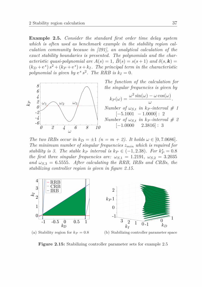
2 Stability region calculation 37
Example 2.5. Consider the standard first order time delay systemwhich is often used as benchmark example in the stability region cal-culation community because in [291], an analytical calculation of theexact stability boundaries is presented. The polynomials and the char-acteristic quasi-polynomial are A(s) = 1, B(s) = s(s + 1) and δ(s, k) =(kD + es) s2 + (kP + es) s + kI . The principal term in the characteristicpolynomial is given by es s2. The RRB is kI = 0.
0 2 4 6 8 10-6-4-202468
ω
ω3ω2ω1kP
The function of the calculation forthe singular frequencies is given by
kP (ω) =ω2 sin(ω)− ω cos(ω)
ω.
Number of ωS,t in kP -interval # 1aaaa [−5.1001 − 1.0000] : 2Number of ωS,t in kP -interval # 2aaaa [−1.0000 2.3816] : 3
The two IRBs occur in kD = ±1 (n = m + 2). It holds ω ∈ [0, 7.0686].The minimum number of singular frequencies zmin which is required forstability is 3. The stable kP interval is kP ∈ (−1, 2.38). For k∗
P = 0.8the first three singular frequencies are: ωS,1 = 1.2191, ωS,2 = 3.2035and ωS,3 = 6.5555. After calculating the RRB, IRBs and CRBs, thestabilizing controller region is given in figure 2.15.
(a) Stability region for kP = 0.8
-10 1
0123-1
0
1
2
kP
kDkI
(b) Stabilizing controller parameter space
Figure 2.15: Stabilizing controller parameter sets for example 2.5
38 2.3 Parameter space approach
Remark:16 In the results presented so far, an ideal PID controller hasbeen considered. In the case of a real PID controller GC(s, k) = kP +kI/s + (kD s)/(TP s + 1), the characteristic equation becomes
δ(s, k, q = B(s, q)(TP s2+s)+A(s, q)((TP kP +kD)s2+(TP kI+kP )s+kI).
The RRB is the same as in the case of an ideal PID controller. TheIRB, changes a bit. By using the characteristic equation it holds:
δ(|s| → ∞, k, q) = es τ + (am TP kP + kD)/(bn TP )
This equation is used similarly to the ideal PID case to build the IRB:
±(TP bn)/(am) = TP kP + kD
This represents two parallel lines in the kP /kD plane. In contrast tothe case of an ideal PID, this equation is a function in kD and kP . Forthe CRB calculation, the characteristic equation results in(�δ
�δ
)=(�A − ωTP�A −ω2�A
�A + ωTP�A −ω2�A
)(kI
kD
)+(−TP ω2�A − ω�A
−TP ω2�A + ω�A
)kP
+(�B(−TP ω2)−�B ω
�B(−TP ω2) + �B ω
)=(
00
).
The solution of this equation set iskP + TP kI = (�B(TP ω�A −�A)−�B(TP ω�A + �A))/(�2
A + �2A).
In the following the substitution of kE = kP + TP kI is used based on[173]. Therefore, for each fixed value k∗
E , one singular frequency resultswhich corresponds to one linear CRB equation based on
�δ : c = (TP ω2 + ω�A/�N )kE + TP ω2 �B/�A + ω�B/�A
�δ : c = (TP ω2 − ω�A/�A)kE + TP ω2 �B/�A − ω�B/�A
with c = (1 + T 2P ω2)kI − ω2 kD. Tuning approaches presented in detail
in [225, 322] can be used for finding the best fitting value of the filterconstant inside the resulting stability region.16A first implementation and discussion of the proposed ideas has been presented
in [S01]. The following section is based on this.
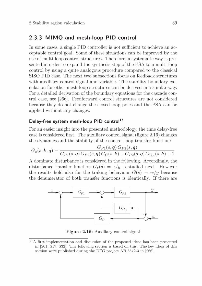
2 Stability region calculation 39
2.3.3 MIMO and mesh-loop PID controlIn some cases, a single PID controller is not sufficient to achieve an ac-ceptable control goal. Some of these situations can be improved by theuse of multi-loop control structures. Therefore, a systematic way is pre-sented in order to expand the synthesis step of the PSA to a multi-loopcontrol by using a quite analogous procedure compared to the classicalSISO PID case. The next two subsections focus on feedback structureswith auxiliary control signal and variable. The stability boundary cal-culation for other mesh-loop structures can be derived in a similar way.For a detailed derivation of the boundary equations for the cascade con-trol case, see [266]. Feedforward control structures are not consideredbecause they do not change the closed-loop poles and the PSA can beapplied without any changes.
Delay-free system mesh-loop PID control17
For an easier insight into the presented methodology, the time delay-freecase is considered first. The auxiliary control signal (figure 2.16) changesthe dynamics and the stability of the control loop transfer function:
Gz(s, k, q) =GP 1(s, q) GP 2(s, q)
GP 1(s, q) GP 2(s, q) GC(s, k) + GP 2(s, q) GCA(s, k) + 1
A dominate disturbance is considered in the following. Accordingly, thedisturbance transfer function Gz(s) = z/y is studied next. Howeverthe results hold also for the traking behaviour G(s) = w/y becausethe denumerator of both transfer functions is identically. If there are
Figure 2.16: Auxiliary control signal
17A first implementation and discussion of the proposed ideas has been presentedin [S01, S17, S32]. The following section is based on this. The key ideas of thissection were published during the DFG project AB 65/2-3 in [266].
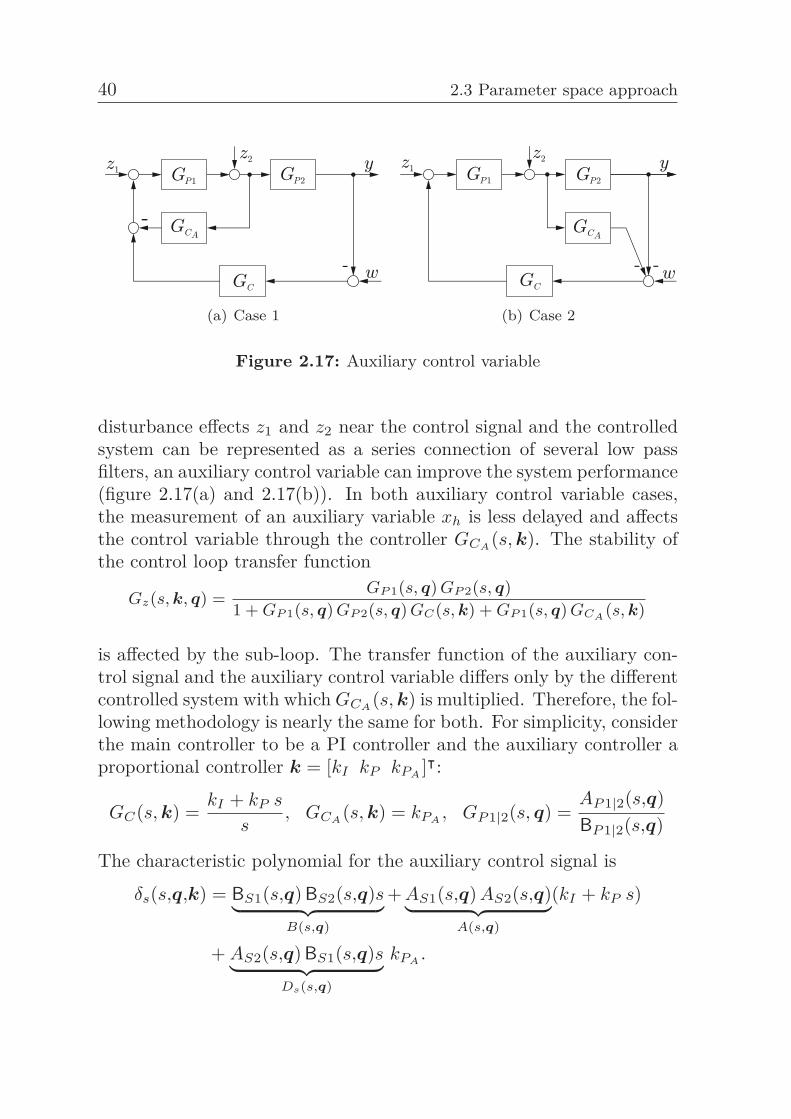
40 2.3 Parameter space approach
(a) Case 1 (b) Case 2
Figure 2.17: Auxiliary control variable
disturbance effects z1 and z2 near the control signal and the controlledsystem can be represented as a series connection of several low passfilters, an auxiliary control variable can improve the system performance(figure 2.17(a) and 2.17(b)). In both auxiliary control variable cases,the measurement of an auxiliary variable xh is less delayed and affectsthe control variable through the controller GCA
(s, k). The stability ofthe control loop transfer function
Gz(s, k, q) = GP 1(s, q) GP 2(s, q)1 + GP 1(s, q) GP 2(s, q) GC(s, k) + GP 1(s, q) GCA (s, k)
is affected by the sub-loop. The transfer function of the auxiliary con-trol signal and the auxiliary control variable differs only by the differentcontrolled system with which GCA
(s, k) is multiplied. Therefore, the fol-lowing methodology is nearly the same for both. For simplicity, considerthe main controller to be a PI controller and the auxiliary controller aproportional controller k = [kI kP kPA
]ᵀ:
GC(s, k) =kI + kP s
s, GCA
(s, k) = kPA, GP 1|2(s, q) =
AP 1|2(s,q)BP 1|2(s,q)
The characteristic polynomial for the auxiliary control signal is
δs(s,q,k) = BS1(s,q) BS2(s,q)s︸ ︷︷ ︸B(s,q)
+ AS1(s,q) AS2(s,q)︸ ︷︷ ︸A(s,q)
(kI + kP s)
+ AS2(s,q) BS1(s,q)s︸ ︷︷ ︸Ds(s,q)
kPA.
2 Stability region calculation 41
In case of an auxiliary control variable it results
δv(s,q,k) = BS1(s,q) BS2(s,q)s︸ ︷︷ ︸B(s,q)
+ AS1(s,q) AS2(s,q)︸ ︷︷ ︸A(s,q)
(kI + kP s)
+ AS1(s,q) BS2(s,q)s︸ ︷︷ ︸Dv(s,q)
kPA
with the polynomial Ds|v(s,q) = d0(q) + . . . + ds|v,mD(q)smD with
ds|v,mD(q) �= 0, where mD is the order of the polynomial Ds|v(s,q).
Real root boundary Similar to the previous cases, substituting s = 0into δs|v(s, k, q∗) gives the RRB equation:
δs|v(0,k,q∗) = B(s = 0,q∗) + A(s = 0,q∗) kI + Ds|v(s = 0, q∗) kPA= 0
⇒ kI = −b0 + ds|v,0 kPA
a0(2.15)
The result is a straight line in the controller parameter space. Theequation is always zero in the present PI control case (⇒ b0 = d0 = 0).
Infinite root boundary All terms which do not have a maximum powerof s are deleted. For the IRB calculation, the characteristic equation be-comes δs|v(|s| → ∞, k, q∗) = bn sn + kP s am sm + kPA
ds|v,mDsmD . To
calculate the IRB equations the following two cases must be studied
for mD < n⇒
⎧⎪⎪⎨⎪⎪⎩kP = 0 for n < m + 1kP = − bn
amfor n = m + 1
∅ for n > m + 1,
for mD = n⇒
⎧⎪⎪⎨⎪⎪⎩kP = 0 for n < m + 1kP = − bn+ds|v,mD
kPA
amfor n = m + 1
kPA= − bn
ds|v,mD
for n > m + 1.
(2.16)
The case mD > n does not exist.
42 2.3 Parameter space approach
Complex root boundaries After the substitution of s = jω, ω ∈ R+
into δs|v(s, k, q∗) = 0, the characteristic polynomial has to be split intoa real and an imaginary part(
�δs|v(ω, k, q∗)
�δs|v(ω, k, q∗)
)=(�A(ω, q∗) −ω�A(ω, q∗)�A(ω, q∗) ω�A(ω, q∗)
)(kI
kP
)
+(�B(ω, q∗)�B(ω, q∗)
)+
(�Ds|v
(ω, q∗)�Ds|v
(ω, q∗)
)kPA
=(
00
).
Since the resulting system of equations is underdetermined, kP is set toa fixed value k∗
P to solve the two equations for kPA
kPA (ω, k∗P , kI , q∗) = k∗
P �A(ω, q∗) ω − kI �A(ω, q∗) − �B(ω, q∗)�Ds|v
(ω, q∗)
kPA (ω, k∗P , kI , q∗) = −kI �A(ω, q∗) + k∗
P �A(ω, q∗) ω + �B(ω, q∗)�Ds|v
(ω, q∗). (2.17)
Equation (2.17) depends on ω and kI . Hence, both equations in theequation set (2.17) must be equal and solved for kI . It results
kI(ω, k∗P , kI , q∗) =
−k∗P �A(ω, q∗) �Ds|v
(ω, q∗) ω + �B(ω, q∗) �Ds|v(ω, q∗)
�A(ω, q∗) �Ds|v(ω, q∗) − �A(ω, q∗) �Ds|v
(ω, q∗)
−k∗
P �A(ω, q∗) �Ds|v(ω, q∗) ω − �B(ω, q∗) �Ds|v
(ω, q∗)�A(ω, q∗) �Ds|v
(ω, q∗) − �A(ω, q∗) �Ds|v(ω, q∗)
. (2.18)
Equation (2.18) is now only a function of ω. The following calculationis similar to the determination of singular frequencies in the previoussections. The obtained value pairs (ωi
S,t, kI(ωiS,t)) can be inserted into
the first or the second row of equation (2.17). The result is a point ofthe complex root boundary in the kPA
/kI plane. For a sufficient numberof pairs, the points can be interpolated to receive the CRB, see figure2.18. In contrast to the SISO PID case, only one point on the CRB andnot one CRB line results for each singular frequency.
Example 2.6. The following example is based on an auxiliary controlsignal scheme with the system transfer functions
GP 1(s, q∗) = 3.5/(1 + 4s) and GP 2(s, q∗) = 2/(1 + 3s).
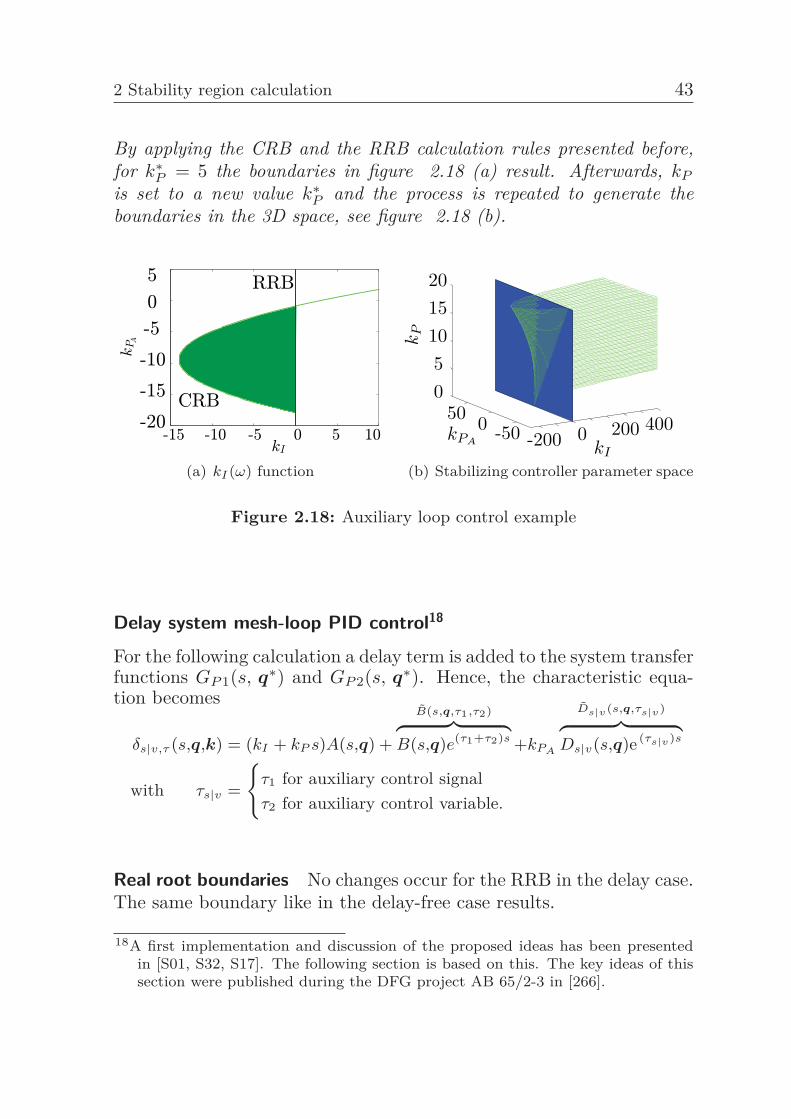
2 Stability region calculation 43
By applying the CRB and the RRB calculation rules presented before,for k∗
P = 5 the boundaries in figure 2.18 (a) result. Afterwards, kP
is set to a new value k∗P and the process is repeated to generate the
boundaries in the 3D space, see figure 2.18 (b).
(a) kI(ω) function
-200 0 200 400-5005005
101520
kI
kPA
kP
(b) Stabilizing controller parameter space
Figure 2.18: Auxiliary loop control example
Delay system mesh-loop PID control18
For the following calculation a delay term is added to the system transferfunctions GP 1(s, q∗) and GP 2(s, q∗). Hence, the characteristic equa-tion becomes
δs|v,τ (s,q,k) = (kI + kP s)A(s,q) +
B(s,q,τ1,τ2)︷ ︸︸ ︷B(s,q)e(τ1+τ2)s +kPA
Ds|v(s,q,τs|v)︷ ︸︸ ︷Ds|v(s,q)e (τs|v)s
with τs|v =
{τ1 for auxiliary control signalτ2 for auxiliary control variable.
Real root boundaries No changes occur for the RRB in the delay case.The same boundary like in the delay-free case results.
18A first implementation and discussion of the proposed ideas has been presentedin [S01, S32, S17]. The following section is based on this. The key ideas of thissection were published during the DFG project AB 65/2-3 in [266].
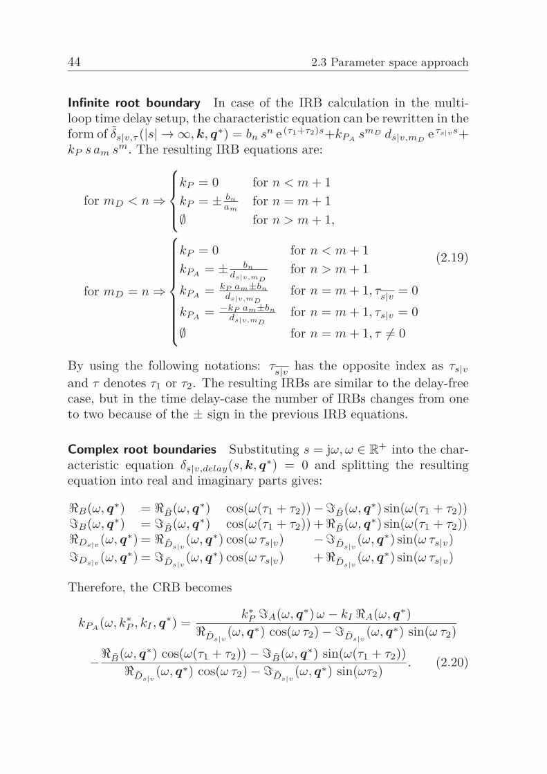
44 2.3 Parameter space approach
Infinite root boundary In case of the IRB calculation in the multi-loop time delay setup, the characteristic equation can be rewritten in theform of δs|v,τ (|s| → ∞, k, q∗) = bn sn e (τ1+τ2)s+kPA
smD ds|v,mDe τs|vs+
kP s am sm. The resulting IRB equations are:
for mD < n⇒
⎧⎪⎪⎨⎪⎪⎩kP = 0 for n < m + 1kP = ± bn
amfor n = m + 1
∅ for n > m + 1,
for mD = n⇒
⎧⎪⎪⎪⎪⎪⎪⎪⎪⎨⎪⎪⎪⎪⎪⎪⎪⎪⎩
kP = 0 for n < m + 1kPA
= ± bn
ds|v,mD
for n > m + 1kPA
= kP am±bn
ds|v,mD
for n = m + 1, τs|v = 0
kPA= −kP am±bn
ds|v,mD
for n = m + 1, τs|v = 0∅ for n = m + 1, τ �= 0
(2.19)
By using the following notations: τs|v has the opposite index as τs|v
and τ denotes τ1 or τ2. The resulting IRBs are similar to the delay-freecase, but in the time delay-case the number of IRBs changes from oneto two because of the ± sign in the previous IRB equations.
Complex root boundaries Substituting s = jω, ω ∈ R+ into the char-
acteristic equation δs|v,delay(s, k, q∗) = 0 and splitting the resultingequation into real and imaginary parts gives:
�B(ω, q∗) = �B(ω, q∗) cos(ω(τ1 + τ2))−�B(ω, q∗) sin(ω(τ1 + τ2))�B(ω, q∗) = �B(ω, q∗) cos(ω(τ1 + τ2)) +�B(ω, q∗) sin(ω(τ1 + τ2))�Ds|v
(ω, q∗) = �Ds|v(ω, q∗) cos(ω τs|v) −�Ds|v
(ω, q∗) sin(ω τs|v)�Ds|v
(ω, q∗) = �Ds|v(ω, q∗) cos(ω τs|v) +�Ds|v
(ω, q∗) sin(ω τs|v)
Therefore, the CRB becomes
kPA(ω, k∗
P , kI , q∗) =k∗
P �A(ω, q∗) ω − kI �A(ω, q∗)�Ds|v
(ω, q∗) cos(ω τ2)−�Ds|v(ω, q∗) sin(ω τ2)
−�B(ω, q∗) cos(ω(τ1 + τ2))−�B(ω, q∗) sin(ω(τ1 + τ2))�Ds|v
(ω, q∗) cos(ω τ2)−�Ds|v(ω, q∗) sin(ωτ2)
. (2.20)
2 Stability region calculation 45
After generating the CRB equations, the presented approach for thedelay-free case can be applied to plot the CRBs. One difference tothe delay-free case is the trigonometric functions in the resulting CRBequation. Therefore, an infinite number of kI/ω pairs results. Also, aninfinite number of (kI(ωS,t), ωS,t) pairs results. Actually, all the result-ing points on the CRB belong to one very long tortuoused CRB curve.In contrast to the classical PID single-loop time delay parameter spaceapproach, only one CRB in the delay-free case and in the delay caseexist. This CRB is nonlinear. As a consequence, the resulting stablecontroller area does not have to be a convex polygon.The implementation of some general plotting rules is a problem. TheCRB plotting problem in higher order cases can be reformulated by us-ing the two continuous functions f1(kα, kβ , ω) = 0 and f2(kα, kβ , ω) = 0where kα and kβ are the free controller parameters. All other controllerparameters are fixed. In some special cases, this problem can be analyti-cally solved by using elimination methods for sets of nonlinear equations[78]. D. Kaesbauer [167] and A. Reiter [253] are discussing different ap-proaches (like the Resultant method) in the context of the delay-freePSA. Some Gröbner basis-based approaches also exist and are appli-cable for delay systems which approximate the trigonometric functionsby rational functions [185]. More generally applicable but without anaccuracy guaranty is the numerical parameter sweeping method to de-couple and plot the equations. However, in the case of high dimensionalproblems, the PSA calculation becomes very complex and the practicaluse is questionable.
Decoupling based MIMO control 19
In this section, MIMO systems with high interactions among the inputand the output variables are studied, e.g. detected by relative gain ar-ray study. A classical approach to design multi-variable controllers isthe use of pre-compensators (decoupler) that convert the MIMO systeminto several decoupled, decentralized SISO systems by transferring thesystem matrix into a diagonal form. Thereafter, the SISO controllerdesign can be applied, like in section 2.3.1 and 2.3.2. D. Rosinova and
19A first implementation and discussion of the proposed ideas has been presented in[S18]. The following section is based on this. The key ideas of this section werepublished during the DFG project AB 65/2-3 in [274].
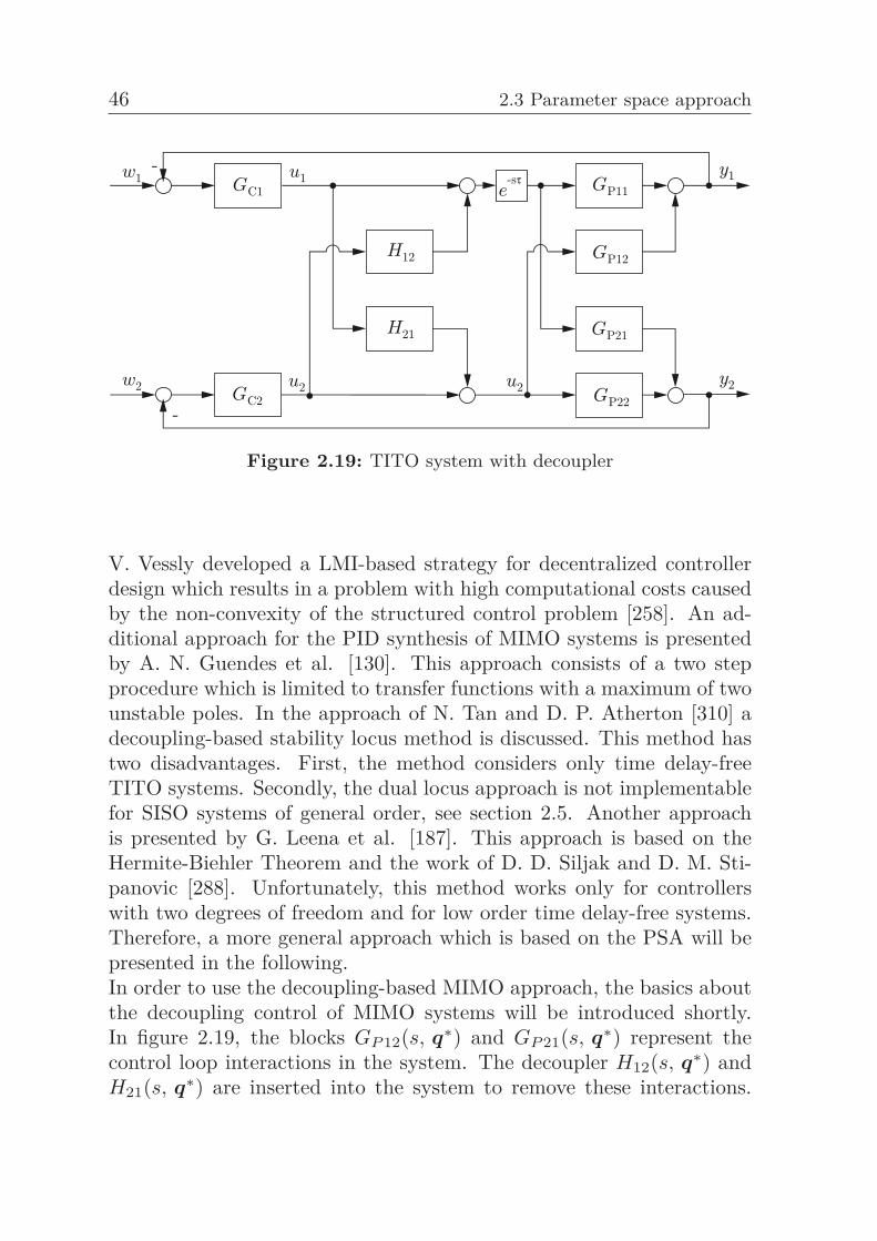
46 2.3 Parameter space approach
Figure 2.19: TITO system with decoupler
V. Vessly developed a LMI-based strategy for decentralized controllerdesign which results in a problem with high computational costs causedby the non-convexity of the structured control problem [258]. An ad-ditional approach for the PID synthesis of MIMO systems is presentedby A. N. Guendes et al. [130]. This approach consists of a two stepprocedure which is limited to transfer functions with a maximum of twounstable poles. In the approach of N. Tan and D. P. Atherton [310] adecoupling-based stability locus method is discussed. This method hastwo disadvantages. First, the method considers only time delay-freeTITO systems. Secondly, the dual locus approach is not implementablefor SISO systems of general order, see section 2.5. Another approachis presented by G. Leena et al. [187]. This approach is based on theHermite-Biehler Theorem and the work of D. D. Siljak and D. M. Sti-panovic [288]. Unfortunately, this method works only for controllerswith two degrees of freedom and for low order time delay-free systems.Therefore, a more general approach which is based on the PSA will bepresented in the following.In order to use the decoupling-based MIMO approach, the basics aboutthe decoupling control of MIMO systems will be introduced shortly.In figure 2.19, the blocks GP 12(s, q∗) and GP 21(s, q∗) represent thecontrol loop interactions in the system. The decoupler H12(s, q∗) andH21(s, q∗) are inserted into the system to remove these interactions.
2 Stability region calculation 47
The MIMO input-output equations are:
y1 = u1(GP 11(s, q∗) + GP 12(s, q∗) H21(s, q∗)) + u2(GP 12(s, q∗)+ GP 11(s, q∗) H12(s, q∗))
y2 = u2(GP 22(s, q∗) + GP 21(s, q∗) H12(s, q∗)) + u1(GP 21(s, q∗)+ GP 22(s, q∗) H21(s, q∗))
After eliminating the effect of u2 on y1 the following condition mustsatisfy GP 12(s, q∗) + GP 11(s, q∗) H12(s, q∗) = 0 which finally yields:H12(s, q∗) = −GP 12(s, q∗) / GP 11(s, q∗). Analogically, for the elimi-nation of the effect of u1 on y2, the decoupler H21(s, q∗) becomes:H21(s, q∗) = −GP 21(s, q∗) / GP 22(s, q∗). For decoupling systems withtime delays, it is required to ensure that the resulting decoupler arephysically realizable. Supposing that G12(s, q∗) = GP 12(s, q∗)e−τ12s
and G11(s, q∗) = GP 11(s, q∗)e−τ11s, the decoupler equations becomes:
H12(s, q∗) = −GP 12(s, q∗) e−τ12s
GP 11(s, q∗) e−τ11s= −GP 12(s, q∗)
GP 11(s, q∗)e−(τ12−τ11)s
H21(s, q∗) = −GP 21(s, q∗) e−τ21s
GP 22(s, q∗) e−τ22s= −GP 21(s, q∗)
GP 22(s, q∗)e−(τ21−τ22)s
The configuration of decoupler results in one of the following four casesdepending on the value of each time delay for TITO systems:
• τ12 > τ11 and τ21 > τ22: The resulting decoupler is realizable.The decoupling for time delay systems is done in the same way asit is done for time delay-free systems.
• τ11 = τ12 and τ22 = τ21: The time delay is canceled.• τ12 < τ11 and τ21 < τ22: In this case, the system is unrealizable.
One way to solve this is to change the inputs in figure 2.19 in such away that the input u1 controls the output y2 and the input u2 con-trols the output y1. Thereafter, the numerators and denominatorsof the decoupler are switched and the decoupler H11(s, q∗) be-comes H21(s, q∗) = GP 11(s, q∗) / GP 12(s, q∗). Similarly decou-pler H12(s, q∗) becomes H12(s, q∗) = −GP 22(s, q∗) / GP 21(s, q∗).
• τ12 < τ11 or τ21 < τ22: Only one decoupler is realizable in his case.The input cannot be switched like in the third case. In order to
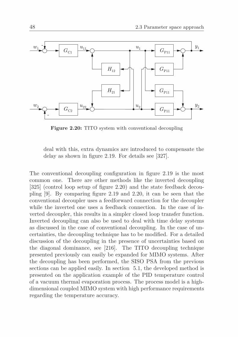
48 2.3 Parameter space approach
Figure 2.20: TITO system with conventional decoupling
deal with this, extra dynamics are introduced to compensate thedelay as shown in figure 2.19. For details see [327].
The conventional decoupling configuration in figure 2.19 is the mostcommon one. There are other methods like the inverted decoupling[325] (control loop setup of figure 2.20) and the state feedback decou-pling [9]. By comparing figure 2.19 and 2.20, it can be seen that theconventional decoupler uses a feedforward connection for the decouplerwhile the inverted one uses a feedback connection. In the case of in-verted decoupler, this results in a simpler closed loop transfer function.Inverted decoupling can also be used to deal with time delay systemsas discussed in the case of conventional decoupling. In the case of un-certainties, the decoupling technique has to be modified. For a detaileddiscussion of the decoupling in the presence of uncertainties based onthe diagonal dominance, see [216]. The TITO decoupling techniquepresented previously can easily be expanded for MIMO systems. Afterthe decoupling has been performed, the SISO PSA from the previoussections can be applied easily. In section 5.1, the developed method ispresented on the application example of the PID temperature controlof a vacuum thermal evaporation process. The process model is a high-dimensional coupled MIMO system with high performance requirementsregarding the temperature accuracy.
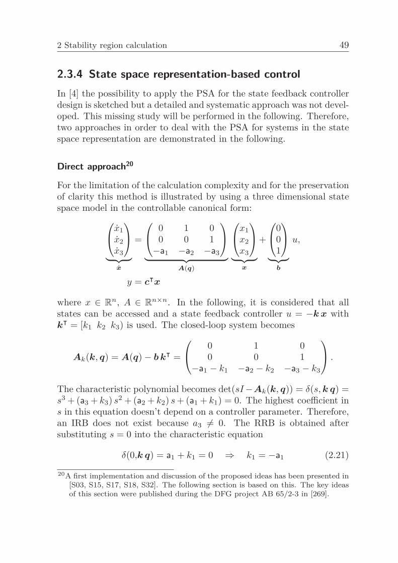
2 Stability region calculation 49
2.3.4 State space representation-based controlIn [4] the possibility to apply the PSA for the state feedback controllerdesign is sketched but a detailed and systematic approach was not devel-oped. This missing study will be performed in the following. Therefore,two approaches in order to deal with the PSA for systems in the statespace representation are demonstrated in the following.
Direct approach20
For the limitation of the calculation complexity and for the preservationof clarity this method is illustrated by using a three dimensional statespace model in the controllable canonical form:⎛⎝x1
x2x3
⎞⎠︸ ︷︷ ︸
x
=
⎛⎝ 0 1 00 0 1−a1 −a2 −a3
⎞⎠︸ ︷︷ ︸
A(q)
⎛⎝x1x2x3
⎞⎠︸ ︷︷ ︸
x
+
⎛⎝001
⎞⎠︸ ︷︷ ︸
b
u,
y = cᵀx
where x ∈ Rn, A ∈ R
n×n. In the following, it is considered that allstates can be accessed and a state feedback controller u = −k x withkᵀ = [k1 k2 k3) is used. The closed-loop system becomes
Ak(k, q) = A(q)− b kᵀ =
⎛⎝ 0 1 00 0 1
−a1 − k1 −a2 − k2 −a3 − k3
⎞⎠ .
The characteristic polynomial becomes det(sI−Ak(k, q)) = δ(s, k q) =s3 + (a3 + k3) s2 + (a2 + k2) s + (a1 + k1) = 0. The highest coefficient ins in this equation doesn’t depend on a controller parameter. Therefore,an IRB does not exist because a3 �= 0. The RRB is obtained aftersubstituting s = 0 into the characteristic equation
δ(0,k q) = a1 + k1 = 0 ⇒ k1 = −a1 (2.21)
20A first implementation and discussion of the proposed ideas has been presented in[S03, S15, S17, S18, S32]. The following section is based on this. The key ideasof this section were published during the DFG project AB 65/2-3 in [269].
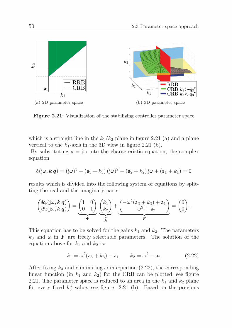
50 2.3 Parameter space approach
(a) 2D parameter space (b) 3D parameter space
Figure 2.21: Visualization of the stabilizing controller parameter space
which is a straight line in the k1/k2 plane in figure 2.21 (a) and a planevertical to the k1-axis in the 3D view in figure 2.21 (b).By substituting s = jω into the characteristic equation, the complex
equation
δ(jω, k q) = (jω)3 + (a3 + k3) (jω)2 + (a2 + k2) jω + (a1 + k1) = 0
results which is divided into the following system of equations by split-ting the real and the imaginary parts(
�δ(jω, k q)�δ(jω, k q)
)=(
1 00 1
)︸ ︷︷ ︸
Φ
(k1k2
)︸ ︷︷ ︸
k
+(−ω2(a3 + k3) + a1−ω2 + a2
)︸ ︷︷ ︸
F
=(
00
).
This equation has to be solved for the gains k1 and k2. The parametersk3 and ω in F are freely selectable parameters. The solution of theequation above for k1 and k2 is:
k1 = ω2(a3 + k3)− a1 k2 = ω2 − a2 (2.22)
After fixing k3 and eliminating ω in equation (2.22), the correspondinglinear function (in k1 and k2) for the CRB can be plotted, see figure2.21. The parameter space is reduced to an area in the k1 and k2 planefor every fixed k∗
3 value, see figure 2.21 (b). Based on the previous
2 Stability region calculation 51
calculations, the parameter space boundaries can be constructed. Un-fortunately, it is unknown which of the resulting polygons is the stableone. This can be solved by using the stability condition of Routh andHurwitz. The first stability condition demands:
a0 > 0 ⇔ k1 > −a1
a1 > 0 ⇔ k2 > −a2
a2 > 0 ⇔ k3 > −a3
(2.23)
for the coefficients a = [a1, a2, a3] of the characteristic equation. Fromequation (2.23) it can be seen that the stable parameter area can only belocated to the right of −a1 (RRB) and above a2, shown in figure 2.21.Furthermore, k1 = −a1 and k2 = −a2 are asymptotes for the positionof the CRB. With increasing k3, the CRB rotates clockwise around thepoint (k1, k2) = (−a1,−a2) from the vertical position (k3 → −a3) to thehorizontal position (k3 →∞). Accordingly, the stable region increases.In addition, k3 > −a3 (k3-limit, in yellow) must be applied. By us-ing the described method, two of the three possible stability areas (seefigure 2.21) can be detected as unstable. Hence, only one stable arearesults (thereby the second condition of Routh and Hurwitz must notbe applied). From the last line in equation (2.23), a condition resultswhich specifies the k3 interval which must be gridded for creating the3D plot (figure 2.21).However, this holds only for the third order case. The calculation com-plexity increases with growing system dimensionality. This can pre-sented easily on an sixth order system in controller canonical form witha state feedback controller. Here, the closed-loop system becomes
Ak =
⎛⎜⎜⎜⎜⎜⎝0 1 0 0 0 00 0 1 0 0 00 0 0 1 0 00 0 0 0 1 00 0 0 0 0 1
−a1 − k1 −a2 − k2 −a3 − k3 −a4 − k4 −a5 − k5 −a6 − k6
⎞⎟⎟⎟⎟⎟⎠Based on this, the characteristic polynomial becomes δ(s, k q) = s6 +(a6 + k6) s5 + (a4 + k4) s4 + (a3 + k3) s2 + (a2 + k2) s + (a1 + k1). Similarto the previous case, an IRB does not exist because a6 �= 0 and the
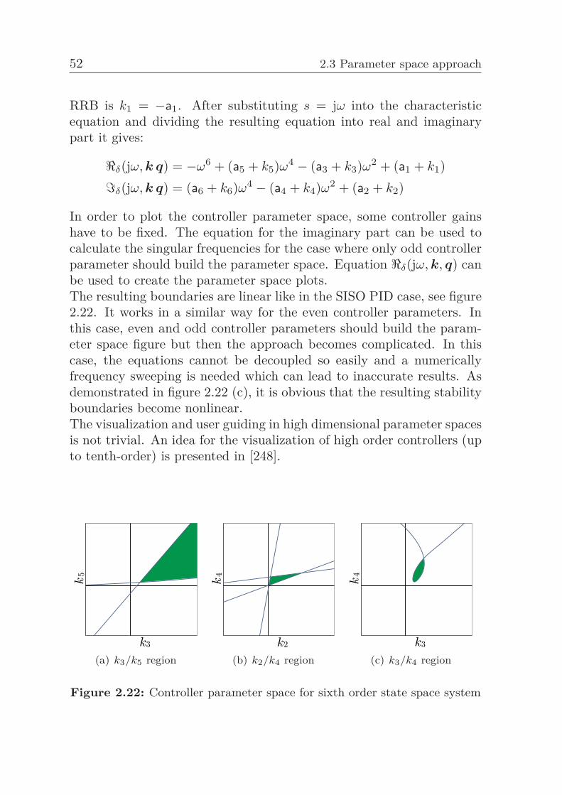
52 2.3 Parameter space approach
RRB is k1 = −a1. After substituting s = jω into the characteristicequation and dividing the resulting equation into real and imaginarypart it gives:
�δ(jω, k q) = −ω6 + (a5 + k5)ω4 − (a3 + k3)ω2 + (a1 + k1)�δ(jω, k q) = (a6 + k6)ω4 − (a4 + k4)ω2 + (a2 + k2)
In order to plot the controller parameter space, some controller gainshave to be fixed. The equation for the imaginary part can be used tocalculate the singular frequencies for the case where only odd controllerparameter should build the parameter space. Equation �δ(jω, k, q) canbe used to create the parameter space plots.The resulting boundaries are linear like in the SISO PID case, see figure2.22. It works in a similar way for the even controller parameters. Inthis case, even and odd controller parameters should build the param-eter space figure but then the approach becomes complicated. In thiscase, the equations cannot be decoupled so easily and a numericallyfrequency sweeping is needed which can lead to inaccurate results. Asdemonstrated in figure 2.22 (c), it is obvious that the resulting stabilityboundaries become nonlinear.The visualization and user guiding in high dimensional parameter spacesis not trivial. An idea for the visualization of high order controllers (upto tenth-order) is presented in [248].
(a) k3/k5 region (b) k2/k4 region (c) k3/k4 region
Figure 2.22: Controller parameter space for sixth order state space system
2 Stability region calculation 53
Algebraic Riccati equation-based approach21
This section presents a method to determine the space of stabilizingcontroller parameters based on the algebraic Riccati equation study ofM. L. Muhler [211]. This is given by
P RP −Aᵀ(k, q)P + P A(k, q) + Q = 0 (2.24)
with A ∈ Rn×n, P ∈ R
n×n, Q ∈ Rn×n, R ∈ R
n×n and R = bbᵀ. Inorder to solve the previous equation the matrix
Z(k, q) =[−A(k, q) R
Q Aᵀ(k, q)
](2.25)
is introduced which is known as a Hamiltonian matrix of the size 2n×2n. An important property of equation (2.25) is that all eigenvalues ofZ(k, q) are symmetric about the imaginary axis. If the condition aboveis satisfied, the RRB, the CRB and the IRB can be calculated. For theRRB the corresponding mapping equation is
det(sI −Z(k, q))|s=0 = 0. (2.26)
The IRB can be obtained similar
det(sI −Z(k, q))|s=∞ = 0. (2.27)
In the case of the CRB two mapping CRB equations exist:
det(sI −Z(k, q))|s=jω = 0 (2.28a)
∂
∂wdet(sI −Z(k, q))|s=jω = 0 (2.28b)
due to the fact that a double eigenpair crosses the imaginary axis twicedue to the appearance of A(k, q) in the diagonal of equation (2.25).After the boundaries are calculated, they are plotted in order to obtainthe space of stabilizing controller parameters.
21A first implementation and discussion of the proposed ideas has been presented in[S15, S18]. The following section is based on this. The key ideas of this sectionwere published during the DFG project AB 65/2-3 in [268,269].
54 2.4 Hermite-Biehler theorem-based approach
Again this version of the PSA is based on frequency sweeping to com-pute the CRBs. Therefore, the same stability boundary equation schemehas to be used as presented in the Direct approach. A very similar ap-proach for the state feedback-based parameter space calculation hasbeen presented in [124]. This approach has the same drawback re-garding the frequency sweeping. An interesting feature of the PSAapproach which is based on the algebraic Riccati equation which M. L.Muhler presented in [211] is the possibility to extend the approach forH∞ performance mapping. The classical H∞ (presented in section 4.4)controller design is based on a linear matrix inequality (LMI) formu-lation. By using the mapping idea of M. L. Muhler the LMIs can bemapped into the parameter space. This offers the possibility to handleunstructured uncertainties with the PSA. Due to the required frequencysweeping the approach becomes complex for high dimensional problemsand cannot be formulated for general problems. A similar approach hasalso been developed by [43,125,145].In [211], M. L. Muhler presented the possibility to map internal qualitycontrol (IQC) constraints in the parameter space by using his mappingapproach. IQCs are very flexible. They offer the possibility to com-bine different design criteria by using a variety of multipliers. However,for the case of parametric uncertainties, the PSA is less conservativein comparison to the IQC or H∞ approaches as well μ-synthesis [134].The IQCs can be transformed into LMIs and utilized to optimize thecontroller gains. As in the previous case, the approach becomes com-plex for high dimensional problems due to the frequency sweeping andcannot be formulated for general problems. In addition, the IQC ro-bust controller synthesis approach has been presented by J. Veenmanand C. W. Scherer in [318]. Their approach is based on the Youla-Kucera parametrization and they showed how flexible IQCs for robustcontroller syntheses are. From a computational point of view, this ap-proach is much more efficient in comparison to M. L. Muhlers PSAmapping method.
2.4 Hermite-Biehler theorem-based approachNext, the classical parameter space calculation approach based on theHermite-Biehler theorem (HBT) is presented briefly, with reference to[292]. This approach is based on Nyquist plots to determine the stability
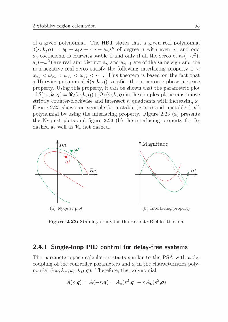
2 Stability region calculation 55
of a given polynomial. The HBT states that a given real polynomialδ(s, k, q) = a0 + a1s + · · · + ansn of degree n with even ae and oddao coefficients is Hurwitz stable if and only if all the zeros of ae(−ω2),ao(−ω2) are real and distinct an and an−1 are of the same sign and thenon-negative real zeros satisfy the following interlacing property 0 <ωe1 < ωo1 < ωe2 < ωo2 < · · · . This theorem is based on the fact thata Hurwitz polynomial δ(s, k, q) satisfies the monotonic phase increaseproperty. Using this property, it can be shown that the parametric plotof δ(jω, k, q) = �δ(ω,k, q)+j�δ(ω,k, q) in the complex plane must movestrictly counter-clockwise and intersect n quadrants with increasing ω.Figure 2.23 shows an example for a stable (green) and unstable (red)polynomial by using the interlacing property. Figure 2.23 (a) presentsthe Nyquist plots and figure 2.23 (b) the interlacing property for �δ
dashed as well as �δ not dashed.
(a) Nyquist plot (b) Interlacing property
Figure 2.23: Stability study for the Hermite-Biehler theorem
2.4.1 Single-loop PID control for delay-free systemsThe parameter space calculation starts similar to the PSA with a de-coupling of the controller parameters and ω in the characteristics poly-nomial δ(ω, kP , kI , kD,q). Therefore, the polynomial
A(s,q) = A(−s,q) = Ae(s2,q)− s Ao(s2,q)
56 2.4 Hermite-Biehler theorem-based approach
is applied to decouple the parameters in the characteristic polynomial.Multiplying δ(s, kP , kI , kD,q) A(s,q) = �δ(ω, kI , kD,q) + j�δ(ω, kP ,q)yields that kI and kD appear only in �δ(ω, kI , kD,q) while kP appearsonly in the imaginary part equation �δ(ω, kP ,q). The generalization ofthe HBT is an extension for non-Hurwitz polynomials. The number ofroots of a given polynomial δ(s, k, q) in the OLHP and the ORHP aredefined as l(δ) and r(δ), respectively.More in detail, the generalization of the HBT states that a polynomialδ(s, kP , kI , kD) is Hurwitz stable if and only if σi(δ(s, kP , kI , kD, q)A(s))= n− [l(A(s,q))−r(A(s,q))]. For any polynomial δ(s, k, q), the value ofthe real signature σr(δ) is equal to the value of the imaginary signatureσi(δ) and each of these values is equal to the difference between l(δ)and r(δ). Both of the signatures can be used for root counting and toverify the interlacing property analytically.
Calculation of the stable kP interval22 For a fixed kP , a necessarycondition for the existence of stabilizing kI and kD values can be cal-culated similar to the PSA:
zmin ≥
⎧⎪⎪⎪⎪⎪⎪⎨⎪⎪⎪⎪⎪⎪⎩
∣∣∣∣n −[l(A(s,q)
)− r
(A(s,q)
)]∣∣∣∣2
if n + m is even∣∣∣∣n −[l(A(s,q)
)− r
(A(s,q)
)]∣∣∣∣+ 1
2if n + m is odd
with n and m the degree of δ(s, kP , kI , kD, q) and A(s,q). The real rootdistribution of �δ(ω,kP ,q) corresponds to the different ranges of kP .Using the fact that n − (l(A(s,q)) − r(A(s,q))) is known, the range ofkP for which �δ(ω,kp,q) satisfies the necessary condition zmin can beidentified. However, it has been shown in section 2.3.1 that the HBT-based stabilizing kP interval can be possibly too large sometimes. Dueto the so called stability peaks the kD/kI plane shrinks to a single pointat a certain kP value. This is not considered in the HBT.
22A first implementation and discussion of the proposed ideas has been presented in[S31]. The following section is based on this. The key ideas of this section werepublished during the DFG project AB 65/2-3 in [270].
2 Stability region calculation 57
Finite root boundary calculation23 The string I contains all the pos-sible sequences of signum values referring to the previously mentionedinterlacing property. Each signum value represents the region wherethe stability boundary divides the 2D parameter plane into two halves.Hence, for l boundary lines 2l possibilities of fixed strings I do exist. Butnot all strings I define a region in the kI/kD plane, see the previouslystated stabilizing kP interval as well as the zmin discussions in the caseof the PSA. The sequence of signum values for ωt with t = 0, 1, 2, . . . , lis defined by
it =
{0 if A(ωt,q) = 0α otherwise
with α ∈ {−1,1}. With i0,i1,... defined the string I as the followingsequence of numbers:
I ={
i0,i1,...,il if n + m is eveni0,i1,...,il−1 if n + m is odd
This sequence of signums I is checked for stability using the previoustheorem. The feasible string F ∗
kPwhich defines the stable region is
calculated as a set of signums I satisfying the stability condition. Thestability condition which uses root counting is defined as
n − [l(A(s,q)) − r(A(s,q))] =
⎧⎪⎪⎪⎪⎪⎪⎪⎨⎪⎪⎪⎪⎪⎪⎪⎩
[i0 − 2i1 + 2i2 + · · · +(−1)l−12il−1 + (−1)lil
]if n + m even
(−1)l−1sgn[�δ(∞,kP ,q)
][i0 − 2i1 + 2i2 + · · · +(−1)l−12il−1
]if n + m odd.
(−1)l−1sgn[�δ(∞,kP ,q)
]The root locations of δ(s, kP , kI , kD, q) can be determined by the know-ledge of the zeros of the odd part �δ(ω, kP ,q) and the signs of the evenpart �δ(ω, kI , kD,q). After the calculation of the feasible string F ∗
kPthe
stabilizing kI/kD values are obtained by solving the linear inequalities
23A first implementation and discussion of the proposed ideas has been presented in[S31]. The following section is based on this. The key ideas of this section werepublished during the DFG project AB 65/2-3 in [270].
58 2.4 Hermite-Biehler theorem-based approach
defined as follows:
�δ,1(ωt,q) + (kI − kD ω2S,t)�δ,2(ωt,q) > 0, for it = 1 ,
�δ,1(ωt,q) + (kI − kD ω2S,t)�δ,2(ωt,q) < 0, for it = −1
with the real part defined as �δ(ω, kI , kD,q) = �δ,1(ω,q) + (kI −kD ω2) �δ,2(ω,q). Therefore, ωS,0 represents the RRB and the othercalculated singular frequencies calculated correspond to the CRB in thePSA.
Infinite root boundary24 The IRB is not directly considered in theHBT calculation scheme. But the HBT can be extended for the IRBssimilar to the PSA scheme. As mentioned in the PSA, an IRB exists e.g.for degree[B(s,q)] = degree[A(s,q)] + 1. The real part of the character-istic equation is used for the IRB calculation because at |s| = ∞, onlythe real part exists. Therefore, degree[�δ,1(s,q)] = degree[�δ,2(s,q)]+2.The boundary is calculated as
kD =�∞
δ,1(ω,q)ω2�∞
δ,2(ω,q)
where �∞δ,1(ω,q) and �∞
δ,2(ω,q) are the leading coefficients of the poly-nomials �δ,1(ω,q) and �δ,2(ω,q). After substituting the condition for�δ(ω, kI , kD,q) by using the generalization of the HBT, the sequenceof signums from the feasible string F ∗
kPcan be used to calculate the
stable side:
�δ(ωt,kI ,kD,q) it > 0⇒ −kD i∞ > −�∞
δ,1(ω,q)�∞
δ,2(ω,q)⇒ kD i∞ <
�∞δ,1(ω,q)�∞
δ,2(ω,q)
where i∞ corresponds to the last string in the F ∗kP
set.
24A first implementation and discussion of the proposed ideas has been presented in[S31]. The following section is based on this. The key ideas of this section werepublished during the DFG project AB 65/2-3 in [270].
25A first implementation and discussion of the proposed ideas has been presented in[S31]. The following section is based on this. The key ideas of this section werepublished during the DFG project AB 65/2-3 in [270].
2 Stability region calculation 59
Calculation of stable polygons25 After the calculation of the stabilityboundaries, the stable convex polygons have to be determined. In thecase of the PSA, the stable polygons consider only the regions boundedby the stable boundary sides. By using this approach all of the unsta-ble regions in the kI/kD plane can be eliminated. After this process itis necessary to proceed with a stability test on each resulting polygonwhich satisfies the linear inequalities. This test ensures that the poly-gons are stable. This prevents the detection of wrong stability regionsdue to fictitious boundaries. Therefore, the resulting linear inequalitiesfrom the PSA are only valid for the stable polygons which are boundedby those stability boundaries. After merging all resulting stable poly-gons, the stabilizing set of kI/kD values is calculated in the case of theHBT. The advantage of the HBT is that no additional stability checkis needed for each resulting polygon.
Example 2.7. Consider the plant of example 2.4 with A(s, q∗) = s3 −4s2 + s + 2 and B(s, q∗) = s5 + 8s4 + 32s3 + 46s2 + 46s + 17. The evenand odd parts of the numerator and the denominator are:
Ae(s2, q∗) = −4s2 + 2 and Ao(s2, q∗) = s2 + 1Be(s2, q∗) = 8s4 + 46s2 + 17 and Bo(s2, q∗) = s4 + 32s2 + 46
Consider A(s, q∗) = A(−s, q∗) = Ae(s2, q∗) − sAo(s2, q∗) = (−4s2 +2)− s(s2 + 1) and multiplying A(s) with δ(s, kP , kI , kD, q∗) it gives:
δ(jω,kP ,kI ,kD,q∗) A(jω,q∗) = [�δ,1(ω,q∗) + (kI − kDω2)�δ,2(ω,q∗)]+ j[�δ,1(ω,q∗) + kP�δ,2(ω,q∗)] where
�δ,1(ω,q∗) = −12ω8 + 180ω6 − 183ω4 − 75ω2
�δ,2(ω,q∗) = ω6 + 14ω4 + 17ω2 + 4�δ,1(ω,q∗) = −ω9 + 65ω7 − 246ω5 + 22ω3 + 34ω
�δ,2(ω,q∗) = ω7 + 14ω5 + 17ω3 + 4ω.
The stable range of kP values which satisfies the zmin condition iskP ∈ [−8.5, 4.23337]. For k∗
P = 1 results: �δ(ω,k∗P = 1,q∗) = �δ,1(ω,q∗)
+�δ,2(ω,q∗) = −ω9 + 66ω7 − 232ω5 + 39ω3 + 38ω. Thus, the real non-negative distinct finite zeros of �δ(ω,k∗
P = 1,q∗) with odd multiplicitiesare ω0 = 0, ωS,1 = 0.74230, ωS,2 = 1.86590, ωS,3 = 7.89211. Since
60 2.4 Hermite-Biehler theorem-based approach
n + m = 9 which is odd and A(s) has no roots on the imaginary axis,the set F becomes:
F =
⎧⎪⎪⎪⎪⎪⎪⎪⎪⎪⎪⎨⎪⎪⎪⎪⎪⎪⎪⎪⎪⎪⎩
{−1,− 1,− 1,− 1,0} {1,− 1,− 1,− 1,0}{−1,− 1,− 1,1,0} {1,− 1,− 1,1,0}{−1,− 1,1,− 1,0} {1,− 1,1,− 1,0}{−1,− 1,1,1,0} {1,− 1,1,1,0}{−1,1,− 1,− 1,0} {1,1,− 1,− 1,0}{−1,1,− 1,1,0} {1,1,− 1,1,0}{−1,1,1,− 1,0} {1,1,1,− 1,0}{−1,1,1,1,0} {1,1,1,1,0}
⎫⎪⎪⎪⎪⎪⎪⎪⎪⎪⎪⎬⎪⎪⎪⎪⎪⎪⎪⎪⎪⎪⎭Examining the root distribution of the numerator polynomial A(s) byl(A(s,q∗))−r(A(s,q∗)) = −1 and evaluating the sign of �δ(ω,k∗
P = 1,q∗)at∞ gives (−1)l−1sgn[�δ(∞,1,q∗)] = 1. It follows that every string I ={i0,i1,i2,i3,i4} ∈ F ∗
1 must satisfy the following condition for stability:i0 − 2i1 + 2i2 − 2i3 + i4 = 7. The feasible string F ∗
1 which satisfies thiscondition is determined as F ∗
1 = {1,− 1,1,− 1,0}. Thus, it follows thatthe stabilizing kI/kD values which corresponds to k∗
P = 1 must satisfythe following string of inequalities:⎧⎪⎪⎨⎪⎪⎩
�δ,1(ω0) + (kI − kDω20)�δ,2(ω0) > 0
�δ,1(ω1) + (kI − kDω21)�δ,2(ω1) < 0
�δ,1(ω2) + (kI − kDω22)�δ,2(ω2) > 0
�δ,1(ω3) + (kI − kDω23)�δ,2(ω3) < 0
⇒
⎧⎪⎪⎨⎪⎪⎩kI > 0kI − 0.55101 kD < 3.81670kI − 3.48158 kD > −12.19183kI − 62.2854 kD < 464.03862
The admissible set of kI/kD values can be solved by linear programming.By sweeping over different kP values in the interval (-8.5,4.23337) andfollowing the procedure illustrated above, the whole stabilizing controllerparameter space can be generated and the same controller parameterspace as in example 2.4 results.
2.4.2 Single-loop PID control for delay systems
In the delay-free case, the calculation rules are working quite well forhigh order systems [103,262]. However, for time delay systems, the ex-tension of this approach is not possible in general. In [292], the HBTis extended only to first order systems with time delay. HBT calcula-
2 Stability region calculation 61
tion rules for second order time delay systems are given in [238]. Themethod proposed in [235] provides definitions for the signatures derivedfor quasi-polynomials and also for the stability of time delay systemsusing these signatures. Unfortunately, the modified Nyquist stabilitycriterion which is used in [235] for the calculation of the stabilizing PIDparameter set for delay systems lacks in clarity and cannot be imple-mented as a tool for a plant of arbitrary order. The method of [260] usesan approach similar to [235]. In this publication, the signature defini-tions are simplified and explained in detail. But the stability boundariesand the stability tests are not explained properly. The stable kp intervalis obtained by using the Padé approximation. For the n-th order plantwith time delay where all n poles are identical, the stabilizing regionsof PID controllers can be calculated based on the results of Wang in[329].
Calculation of the stable kP interval26 By using the PSA the range Rand the minimum number of singular frequencies zmin which is requiredfor the stability are defined clearly. Neither the calculation for the stablekP interval nor the stabilizing kI/kD region depend on the order or thestability of the open-loop plant. Using this approach any arbitrary orderplant can be solved for the determination of stabilizing PID controllergains.The generalization of the HBT in [292] uses the results of Pontryaginsimilar to the PSA for first order plants with PID controller. It coversa comprehensive explanation for the stable kP interval and also forthe determination of the stable kI/kD plane for open-loop stable andunstable systems. Unfortunately, the results are difficult to expand ontohigher order systems due to the fact that the approach has no cleardefinition of the limit of singular frequencies. Despite these problemsthe HBT method is a popular method today. This can be seen bythe fact that current control engineering books like [323] are dealingonly with the HBT. In addition, current publications about stabilityregion-based controller tuning are also mainly focusing on the HBT,like [330].26A first implementation and discussion of the proposed ideas has been presented in
[S31]. The following section is based on this. The key ideas of this section werepublished during the DFG project AB 65/2-3 in [270].
62 2.4 Hermite-Biehler theorem-based approach
Conservativeness study27 Consider example 2.7 with a delay of 1 sec.The results given in [292] provide the calculation rules for the stabilityboundaries. The condition for the stability is calculated by using theNyquist stability condition (similarly to the root locus section) wherethe phase and the magnitude conditions are applied to the open-looptransfer function, given by:
1. ∠
((kI − kDω2 + jkP ω) A(jω,q)
sB(jω,q)
)− τω = −π,
⇒ τ(ω) =π + arg
{[(kI − kDω2) + jkP ω] A(jω,q)
jωB(jω,q)
}ω
2.
∣∣∣∣∣(kI − kDω2 + jkP ω) A(jω,q)jωB(jω,q)
∣∣∣∣∣ = 1
⇒ kI − kDω2 = ±
√√√√∣∣∣∣∣ A(jω,q)jωB(jω,q)
∣∣∣∣∣2
− (kP ω)2
For a fixed kP , the second condition can be written as kI − kDω2 =±√
L(ω,q) where L(ω,q) =∣∣∣A(s,q)/(sB(s,q))
∣∣∣2 − (kpω)2. In this ex-ample, k∗
P = 1. Therefore, the singular frequencies can be calculated byusing the condition above. The τ(ω) plot in [292] shows a discontinuity.This is due to the angle function in MATLAB. This function determinesthe phase angle of complex numbers which is between ±π. This can besolved by using the unwrap function in MATLAB. Eliminating the twofrequencies (resulted by the numerical error), the stable area now in-cludes the two regions shaded in yellow. The stability boundaries whichcorrespond to these frequencies are denoted by the use of the dashedblue and red lines in the figure 2.24. Unfortunately, the yellow regionsare excluded from the stable region again because [292] states that theresulting region has to be a subset of the delay-free stability area. Thisis caused by the two stability boundaries which correspond to the casewhere τ = 0 sec denoted by the black lines.Comparing these results with the PSA, it can be seen that the correctstable region also includes the yellow shaded part. The HBT ignores27A first implementation and discussion of the proposed ideas has been presented in
[S31]. The following section is based on this. The key ideas of this section werepublished during the DFG project AB 65/2-3 in [270].
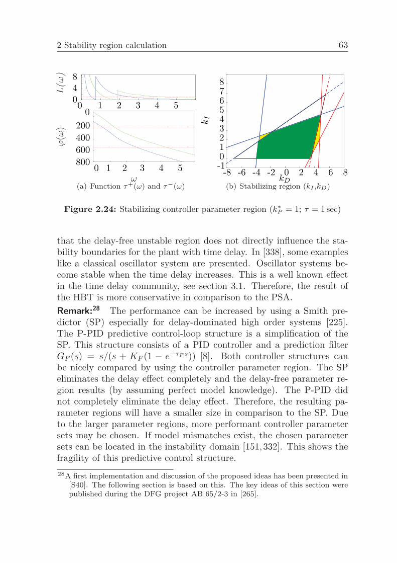
2 Stability region calculation 63
0 1 2 3 4 5048
0 1 2 3 4 5800600400200
0
ω
L(ω
)ϕ
(ω)
(a) Function τ+(ω) and τ−(ω)
-8 -6 -4 -2 0 2 4 6 8-1012345678
kI
kD(b) Stabilizing region (kI ,kD)
Figure 2.24: Stabilizing controller parameter region (k∗P = 1; τ = 1 sec)
that the delay-free unstable region does not directly influence the sta-bility boundaries for the plant with time delay. In [338], some exampleslike a classical oscillator system are presented. Oscillator systems be-come stable when the time delay increases. This is a well known effectin the time delay community, see section 3.1. Therefore, the result ofthe HBT is more conservative in comparison to the PSA.Remark:28 The performance can be increased by using a Smith pre-dictor (SP) especially for delay-dominated high order systems [225].The P-PID predictive control-loop structure is a simplification of theSP. This structure consists of a PID controller and a prediction filterGF (s) = s/(s + KF (1 − e−τF s)) [8]. Both controller structures canbe nicely compared by using the controller parameter region. The SPeliminates the delay effect completely and the delay-free parameter re-gion results (by assuming perfect model knowledge). The P-PID didnot completely eliminate the delay effect. Therefore, the resulting pa-rameter regions will have a smaller size in comparison to the SP. Dueto the larger parameter regions, more performant controller parametersets may be chosen. If model mismatches exist, the chosen parametersets can be located in the instability domain [151,332]. This shows thefragility of this predictive control structure.28A first implementation and discussion of the proposed ideas has been presented in
[S40]. The following section is based on this. The key ideas of this section werepublished during the DFG project AB 65/2-3 in [265].
64 2.5 Alternative Approaches
2.5 Alternative ApproachesRecently used approaches for the parameter space calculation are brieflyintroduced in the following section. Moreover, several expansions of theexisting approaches are presented next.
2.5.1 Dual locus approachOne very popular and often used τ -decomposition approach is the duallocus method [189, 309, 310, 350]. The τ -decomposition method is dis-cussed in detail in [246]. This method is also referred as frequencysweeping. Classically, the delay parameter is of interest and all theother parameters of the system are fixed in this method, see section3.1.1. In the dual locus approach, the stability of time delay systemscan be determined by using Nyquist plots of the systems without delayand the delay element separately. The following calculation explains theall stabilizing PID controller space calculation of time delay systems byusing the dual locus diagram.
Stability boundary calculation29 The method regarding the calcula-tion of all stabilizing gains for the PID controllers for delay systemswhich is based on the dual locus was proposed by J. Li and P. Li [189].The beginning of the calculation scheme is similar to the PSA and theHBT. The characteristic equation for the delay system is
δ(jω, k, q) = �δ(ω) + j�δ(ω, k, q)
with
�δ(ω, k, q) = (kI �A − ω2 kD �A − ω2 kP �A) cos(ω τ)+ ω(kI �A + kP RA − ω2 kD �A) sin(ω τ)− ω2 �B
�δ(ω, k, q) = ω(kI �A + kP �A − ω2 kD �A) cos(ω τ)− (kI RA − ω2 kD RA − ω2 kP �A) sin(ω τ) + ω�B .
Equating�δ(ω, k, q) = 0, �δ(ω, k, q) = 0
29A first implementation and discussion of the proposed ideas has been presentedin [S31]. The following section is based on this.
2 Stability region calculation 65
gives:kP p1(ω) + kI q1(ω) + kD r1(ω) = s1(ω)kP p2(ω) + kI q2(ω) + kD r2(ω) = s2(ω) with
p1(ω) = ω �A sin(ω τ) − ω2 �A cos(ω τ), q1(ω) = �A cos(ω τ) + ω�A sin(ω τ)
r1(ω) = −ω2 �A cos(ω τ) − ω2 �A sin(ω τ), s1(ω) = ω2 �B
p2(ω) = ω �A cos(ω τ) + ω2 �A sin(ω τ), q2(ω) = ω �A cos(ω τ) − �A sin(ωτ)
r2(ω) = ω2 �A sin(ω τ) − ω3 �A cos(ωτ), s2(ω) = −ω2 �B
By assuming kI varies with kD or/and kP , the restrictive assumptionkD = kI/n is used where typically n = 4 holds [189].The stability condition of the system is that the loci of G0(s, k, q, τ = 0)and −e τs have no intersection or that the loci of G0(s, k, q, τ = 0)arrives earlier at the point of intersection than that of −e τs if the twoloci intersect.This is a sufficient but not a necessary condition for the calculation ofstability boundaries. In order to find the closest surface for all stabilizingPID controllers, a unique expression for the parameters kP , kI and kD
as a function of ω must be calculated. The first step is to determinethe frequency ω at which the locus of G0(jω, k, q, τ = 0) intersects withthe unit circle. Based on the previous calculations, the characteristicequation can be reformulated in the following form:
G0 = (kI�A − kD�Aω2 − kP �Aω2) + jω(kI�A − kD�Aω2 − kP �A)−ω2�B + jω�B
If the locus of G0(jω,k,q,τ = 0) intersects with the locus of −e−jωτ , itholds |G0(jω,k,q,τ = 0)| = 1. The frequency ωS,t can be calculated
based on f1ω6 + f2ω4 + f3ω2 + f4 = 0 wheref1 = k2
d I2A, f2 = (kD �A + kP �A)2 −�2
B − 2 kD �A(kI�A + kP �A)f3 = k2
I �2A, f4 = (kI �A + kP �A)2 −�2
B − 2 kI �A(kD �A + kP �A).
The phase angles ϕ1 of G0(s, k, q, τ = 0) and ϕ2 for −e jωτ at ωs are:
ϕ1 = ∠(G0(s, k, q, τ = 0)) = T (kP , kI , kD),ϕ2 = ∠(−e jωsτ ) = ωs τ + π
The argument of G0(s, k, q, τ = 0) = −eτs is the angle between thevector joining the corresponding points on loci G0(s, k, q, τ = 0), −eτs
and the positive real axis. According to this, an additional stability
66 2.5 Alternative Approaches
boundary condition is given by ϕ1 − ϕ2 = 0. All this results in:⎧⎨⎩kP p1(ω) + kI q1(ω) + kD r1(ω) = f5(ω)kP p2(ω) + kI q2(ω) + kD r2(ω) = f6(ω)ϕ1 − ϕ2 = 0
(2.29)
In conclusion, this method is based on the sweeping over frequenciesrather than on the sweeping of parameters of the controller. This ap-proach is easy to implement but does not define the entire stable regionfor the controller parameters. Also the assumption kD = kI/n is veryconservative. Moreover, the fact that the results are presented in thekP /kI plane has serious drawbacks. The boundaries in the kP /kI planeare nonlinear and the shape of the boundaries is hard to predict. There-fore, a detailed study of the boundaries (like shown in section 3.2) basedon the dual locus method would be impossible.
Example 2.8. Consider the same first order delay system as in example2.5. The characteristic equation of the closed-loop transfer function isδ(s, k, q∗) = s(s + 1) + (kDs2 + kP s + kI)e−0.5s. With n = 4 it results:
kP = ω sin(0.5 ω)− cos(0.5 ω)
kI =4 ω [sin(0.5 ω) + ω cos(0.5 ω)]
ω2 + 4
kD =ω [sin(0.5 ω) + ω cos(0.5 ω)
ω2 + 4.
Similar to the RRB, the first stability boundary results by substitutingω = 0 which leads to kI = 0.The stability frequency ωsf = 3.6732 is determined by evaluating the in-tersection point of the delay and the delay-free Nyquist curves, see [189]for a detailed description.Substituting ω from 0 to 3.6732 into the kP , kI and kD equation con-struct the stability boundary. Figure 2.25 (a) shows the stability regionin the kP /kD and the kP /kI plane for τ = [0.2 0.3 0.5 0.8] (the stableregion is the area which is located downwards the curves). The smallestdelay builds the biggest stability region in these example. Figure 2.25(b) presents the whole stabilizing PID parameter space for τ = 0.5 sec.
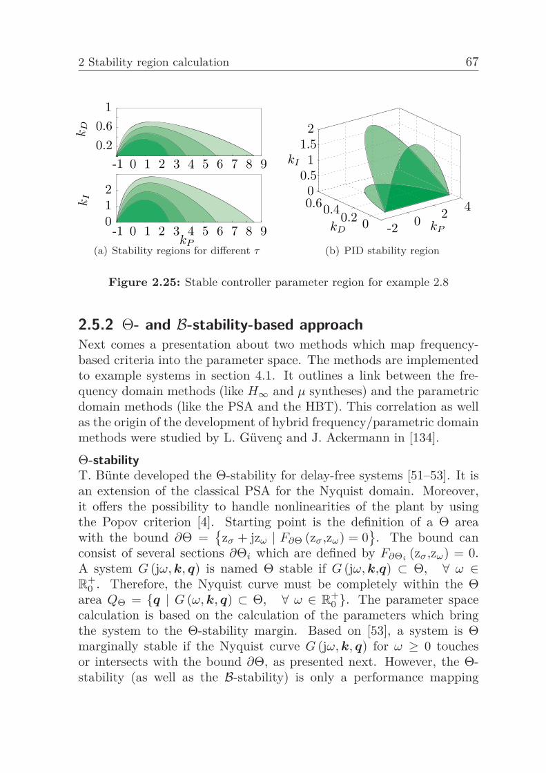
2 Stability region calculation 67
kP
kD
kI
10.60.2
-1 0 1 2 3 4 5 6 7 8 9
210
-1 0 1 2 3 4 5 6 7 8 9(a) Stability regions for different τ
kPkD
kI
21.5
10.500.60.40.2 0 -2 0 2 4
(b) PID stability region
Figure 2.25: Stable controller parameter region for example 2.8
2.5.2 Θ- and B-stability-based approachNext comes a presentation about two methods which map frequency-based criteria into the parameter space. The methods are implementedto example systems in section 4.1. It outlines a link between the fre-quency domain methods (like H∞ and μ syntheses) and the parametricdomain methods (like the PSA and the HBT). This correlation as wellas the origin of the development of hybrid frequency/parametric domainmethods were studied by L. Güvenç and J. Ackermann in [134].
Θ-stabilityT. Bünte developed the Θ-stability for delay-free systems [51–53]. It isan extension of the classical PSA for the Nyquist domain. Moreover,it offers the possibility to handle nonlinearities of the plant by usingthe Popov criterion [4]. Starting point is the definition of a Θ areawith the bound ∂Θ =
{zσ + jzω | F∂Θ (zσ,zω) = 0
}. The bound can
consist of several sections ∂Θi which are defined by F∂Θi (zσ,zω) = 0.A system G (jω, k, q) is named Θ stable if G (jω, k,q) ⊂ Θ, ∀ ω ∈R
+0 . Therefore, the Nyquist curve must be completely within the Θ
area QΘ = {q | G (ω, k, q) ⊂ Θ, ∀ ω ∈ R+0 }. The parameter space
calculation is based on the calculation of the parameters which bringthe system to the Θ-stability margin. Based on [53], a system is Θmarginally stable if the Nyquist curve G (jω, k, q) for ω ≥ 0 touchesor intersects with the bound ∂Θ, as presented next. However, the Θ-stability (as well as the B-stability) is only a performance mapping
68 2.5 Alternative Approaches
technique. To guarantee closed-loop stability, the intersection area ofthe resulting Θ-stability (as well as the B-stability) parameter sets withthe previously presented stabilizing parameter set calculation methodshas to be considered.
Point condition30 In the case of a point condition the Nyquist curveG (jω, k, q) intersects with ∂Θ. Therefore, the parameters are cal-culated which lead to a Nyquist curve that goes to the point z∗ =z∗
σ + jz∗ω ∈ C: Qz∗ = {q,k ∈ R
l | G (jω, k,q) = z∗, ω ∈ R+0 }. By using
the relation G (jω, k,q) = z∗ it follows δ (jω, k,q, z∗) = Gn (jω, k,q) −z∗Gd (jω, k, q) = 0 where Gn (jω, k, q) is the numerator and Gd (jω, k,q)the denominator of the system G (jω, k,q). Then the Nyquist curveG (jω, k,q) goes through the point z∗. The real and imaginary parts ofG (jω, k, q) and z∗ are identical:
�(G (jω, k,q)
)= �
(Gn(jω, k,q)Gd(jω, k, q)
)= � (z∗) = z∗
σ
�(G (jω, k,q)
)= �
(Gn(jω, k,q)Gd(jω, k, q)
)= � (z∗) = z∗
ω
In the literature, those two equations are mapped to the system param-eter space q1/q2 with k = k∗. The two dimensional parameter spaceq1/q2 was used for an easier representation and interpretation of theresults. The previous equation set can be reformulated in the followingform:
p1(ω, k∗,q1, q2
)= �
(Gn
(ω, k∗,q
))− z∗
σ�(
Gd
(ω, k∗, q
))= 0
p2(ω, k∗,q1, q2
)= �
(Gn (ω, k,q)
)− z∗
ω�(
Gd
(ω, k∗, q
))= 0
(2.30)
These equations depend on the three parameters ω, q1 and q2. By usingelimination methods like the Resultant or Gröbner basis method [167],one system parameter can be eliminated:
p3(ω, k∗,q2
)= Res
q1(p1, p2) = 0 (2.31)
30A first implementation and discussion of the proposed ideas has been presentedin [S26]. The following section is based on this.
2 Stability region calculation 69
Thereafter, this equation can be solved for q2 and then substituted intop1. The resulting equation only depends on one system parameter andω. By sweeping over ω, the parameter space can be generated.
Tangent condition31 In the case of a tangent condition, G (jω, k,q)tangents the boundary ∂Θ. Therefore, the Nyquist curve and the Θboundary share a point and have the same slope at this point. By sub-stituting the real part zσ = �
(G (ω, k,q)
)and imaginary part zω =
�(G (ω, k,q)
)into the definition of the Θ boundary, the following con-
ditions result:
F∂Θ
(�(G (ω, k,q1, q2)
),�
(G (ω, k,q1, q2)
))= 0
∂
∂ωF∂Θ
(�(G (ω, k,q1, q2)
),�
(G (ω, k,q1, q2)
))= 0
Based on the mentioned equations, two polynomial equations result:
p1 = numerator[
F∂Θ
(�(G (ω, k,q1, q2)
), �
(G (ω, k,q1, q2)
))]= 0
p2 = ∂
∂ωp1 (ω, k,q1, q2) = 0 (2.32)
Similar to the point condition, the mapping of these two polynomialscan be proceeded.
Expansion for time delay systems32 The Θ-stability approach expan-sion for time delay systems is not easily possible. The polynomials p1and p2 become very large in the delay case. Therefore, the approach isnot applicable for high order delay systems. Moreover, generally appli-cable parameter elimination methods in order to create the polynomialp3 are not available. A general implementation which includes an adap-tive frequency sweeping method is computationally expensive and themapping result is very sensitive for the chosen frequency range and stepsize.
31A first implementation and discussion of the proposed ideas has been presentedin [S26].
32A first implementation and discussion of the proposed ideas has been presentedin [S26]. The following section is based on this.
70 2.5 Alternative Approaches
B-stability
The B-stability maps the frequency domain criterion into the parameterspace by using the amplitude response
∣∣G (jω, k,q)∣∣. This method has
been developed for delay-free systems by D. Odenthal [227,228]. The Bboundaries consist of a lower and an upper bound in order to restrict theamplitude response B with ∂B = |B (jω) |, ω ∈
[ω−, ω+] in the form
|G (jω, k,q) | < |B (jω) | or |G (jω,k, q) | > |B (jω) | ∀ ω ∈[ω−, ω+]. If
the amplitude response is completely inside this bound |G (jω, k, q) | ⊂B, ∀ ω ∈
[ω−, ω+] for ω− ∈ R
+0 , ω+ ∈ R
+0 , the system is B stable. The
stability domain QB is defined as: QB = {q | G (jω, k, q) ⊂ B, ∀ ω ∈[ω−, ω+]}. Similar to the previous section, the following two cases are
studied for the mapping
Point condition33 The point condition maps the case where the ampli-tude response |G (jω, k,q) | and the boundary |B (jω) | are the same fora fixed frequency ω = ω∗ in one point: |G (jω∗, k,q) | = |B (jω∗) |, ∀ q ∈∂QB. Reformulating this equation gives:∣∣G (jω, k,q)
∣∣∣∣B (jω)∣∣ =
∣∣∣∣G (jω, k, q)B (jω)
∣∣∣∣ = 1
By using the definition of the absolute value of a complex number inthe form |�| =
√(� (�)
)2 +(� (�)
)2, it results:
ξ =
(�(
G (jω, k, q)B (jω)
))2
+
(�(
G (jω, k, q)B (jω)
))2
− 1 = 0
with ξ = ξ (ω, q) = (p1 (ω, k, q))/(ξd (ω, k, q)) and ξd (ω, k, q) �= 0. Thepoint condition is mapped for ω = ω∗ into q with:
p1 (ω∗, k,q) = 0 (2.33)
As in the Θ-stability case the parameter mapping of this condition re-sults after applying the frequency sweeping.
33A first implementation and discussion of the proposed ideas has been presentedin [S26].
2 Stability region calculation 71
Tangent condition34 In the case of the tangent condition, the ampli-tude response
∣∣G (jω, k,q)∣∣ touches the boundary
∣∣B (jω)∣∣ tangentially.
In addition to the point condition in equation (2.33), it must hold:
∂∣∣G (jω, k,q)
∣∣∂ω
=∂∣∣B (jω)
∣∣∂ω
⇒ ∂ξ (ω, k, q)∂ω
=∂
∂ω
(p1 (ω, k,q)ξd (ω, k,q)
)By using the quotient rule, the relation
(p1/ξd
)′ = (p′1ξd − p1ξ′
d)/(ξ2d)
results with ξd �= 0 and p2 (ω, q) = p′1 (ω, k, q) = (∂p1 (ω, k,q))/(∂ω).
The tangent condition includes the point condition by using the formu-lation:
p1 (ω, k,q) = 0 and p2 (ω, k, q) = 0 (2.34)
Similar to the Θ-stability case, the equation set (2.34) consists of thethree unknown parameters ω, q1 and q2. By utilizing parameter elimi-nation methods like Resultant or Gröbner basis, an additional equationresults:
p3 (ω, k, q2) = Resq1
(p1, p2,k) = 0 (2.35)By applying the frequency sweeping, the parameter space mapping canbe used similar to the Θ-stability case.
Extension to time delay systems35 For the extension to time delaysystems, two cases have to be considered. In the case of an open-loopcontrol system where the delay term e−jωτ is part of the numerator, nochanges in the initial approach of the B-stability have to be made. Thisis due to the fact that the gain of a transfer function is not affected bythe delay term. Therefore, requirements like the damping ratio can bemapped by using the B-stability. This can be also done by applying theΘ-stability which results in easier mapping equations.The B-stability can also be used to map requirements regarding thesensitivity function. In case of a closed-loop control system, for in-stance when a sensitivity function is examined, the delay term e−jωτ isa part of the denominator. Then, the delay term has to be replaced byEuler’s formula so that the point condition and the tangent conditioncan be examined. Here, the functions p1 and p2 become longer due to34A first implementation and discussion of the proposed ideas has been presented
in [S26].35A first implementation and discussion of the proposed ideas has been presented
in [S26]. The following section is based on this.
72 2.5 Alternative Approaches
the sinus and cosinus term of Euler’s formula. Also the same difficul-ties concerning the complexity of the system arise when the Resultantmethod is used as for the Θ-stability. In contrast, very efficient toolsexist to approximate the solution of the conventional H∞ problem fortime delay systems. However, those solutions are very conservative. Inaddition, the B-stability method is more transparent in comparison tothe classical optimization-based frequency domain methods.
2.5.3 Describing function-based approach
Various methods for checking the stability of nonlinear systems exist.Some of these methods can be theoretically merged with the stabilityregion calculation approaches presented before. The following studiesare based on the assumption that the system can be divided into a lin-ear dynamic and a nonlinear static part. One classical stability analysismethod for such systems is the Popov criterion which is applicable ifthe input-output behavior of the nonlinear part of the system can bedescribed by two sector bounds [7]. These sector bounds can be mappedinto the Nyquist domain for the stability test, see figure 2.26. The or-ange curves are stable but categorized as unstable by some stabilitychecking methods. The resulting bounds in the Nyquist domain can bemapped into the controller parameter space by using the Θ stability.However, this method is conservative and computationally expensivedue to the frequency sweeping. Similarly, the Circle criterion can bemapped into the controller parameter space by using the Θ stability.This reduces the conservatism but the drawback regarding the calcula-tion complexity still holds.A less conservative stability study can be realized by using describingfunctions (harmonic balance method)36. Here, the describing functionof the nonlinear part of the system can be drawn into the Nyquist do-main. The system is stable as long as the describing function does notintersect the Nyquist curve of the linear part of the system [105]. Onepossibility for the mapping into the controller parameter space is againthe use of the Θ stability. An alternative approach is directly based onthe harmonic balance method. Consider the linear part of the system
36A first implementation and discussion of the proposed ideas has been presentedin [S38]. The following section is based on this.
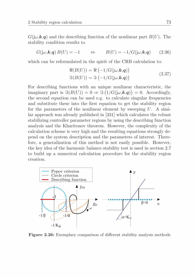
2 Stability region calculation 73
G(jω,k,q) and the describing function of the nonlinear part B(U). Thestability condition results to
G(jω,k,q) B(U) = −1 ⇔ B(U) = −1/G(jω,k,q) (2.36)
which can be reformulated in the spirit of the CRB calculation to:
�(B(U)) = �(−1/G(jω,k,q)
)�(B(U)) = �
(−1/G(jω,k,q)
) (2.37)
For describing functions with an unique nonlinear characteristic, theimaginary part is �(B(U)) = 0 ⇒ �
(1/G(jω,k,q)
)= 0. Accordingly,
the second equation can be used e.g. to calculate singular frequenciesand substitute these into the first equation to get the stability regionfor the parameters of the nonlinear element by sweeping U . A simi-lar approach was already published in [331] which calculates the robuststabilizing controller parameter regions by using the describing functionanalysis and the Kharitonov theorem. However, the complexity of thecalculation scheme is very high and the resulting equations strongly de-pend on the system description and the parameters of interest. There-fore, a generalization of this method is not easily possible. However,the key idea of the harmonic balance stability test is used in section 2.7to build up a numerical calculation procedure for the stability regioncreation.
Figure 2.26: Exemplary comparison of different stability analysis methods
74 2.5 Alternative Approaches
2.5.4 Routh-Hurwitz-based approachAn intuitive idea for the calculation of the stability region could be theRouth-Hurwitz stability criterion. The classical criterion states that acharacteristic polynomial is stable if the Hurwiz matrix [158,259]:
H =
⎡⎢⎢⎢⎢⎢⎢⎢⎢⎢⎢⎢⎢⎢⎢⎢⎢⎢⎢⎢⎣
a1 a3 a5 . . . . . . . . . 0 0 0
a0 a2 a4...
......
a0 a1 a3...
......
... a1 a3... 0
......
... a0 a2. . . an
......
...... a0
. . . an−1 0...
...... 0
. . . an−2 an
......
...... an−3 an−1 0
0 0 0 . . . . . . . . . an−4 an−2 an
⎤⎥⎥⎥⎥⎥⎥⎥⎥⎥⎥⎥⎥⎥⎥⎥⎥⎥⎥⎥⎦
(2.38)
has n leading principle minors larger than zero:
μ1 = det([
a1])
⇒ a1!
> 0
μ2 = det
([a1 a3a0 a2
])⇒ a2 a1 − a0 a3
!> 0 (2.39)
μ3 = det
⎛⎜⎝⎡⎣a1 a3 a5
a0 a2 a40 a1 a3
⎤⎦⎞⎟⎠ ⇒ a3 H − a1(a1 a4 − a0 a5)
!> 0
up to μn = det(H)!> 0. Lets assume that all ai, i = 1, 2, . . . n are a
function of k and q. Thus, the equation set which is based on the Routh-Hurwitz criterion can be solved for the controller parameters of interestwithout numerical frequency sweeping. However, it is only applicablefor LTI delay-free systems and leads to a high computational effort forhigh dimensional systems. In addition, the stability region calculationproduces some fictitious boundaries. The classical D-decomposition ap-proaches like [4] don’t use the Routh-Hurwitz-based condition becausehighly sophisticated symbolic calculation routines are needed to real-ize this mapping. Sophisticated symbolic calculation routines were notavailable in the early days of the D-decomposition.
2 Stability region calculation 75
2.6 Lyapunov stability-based approachIn the following a novel method to compute the stability region by usingthe Lyapunov stability criterion is presented37. A closed-loop systemx = f(x,t) with its equilibrium in the origin is stable based on thesecond method of Lyapunov if a Lyapunov candidate function existsV (x) ≥ 0 with equality if and only if x = 0 which bounds the solutionof the system and fulfills the condition V (x) = ∂
∂t V (x) ≤ 0 with equal-ity not constrained to only x = 0 [171]. For a wide class of systems theproblem of finding a suitable Lyapunov candidate can be reformulatedinto a LMI condition. This is shortly sketched in the following. Con-sider the LTI system x = Akx and the quadratic Lyapunov candidateV (x) = xᵀP x with P > 0. The derivative of the Lyapunov candidatecan be calculated as follows:
V = xᵀP x + xᵀP x = (Akx)ᵀP x + xᵀP (Akx) = xᵀ(AᵀkP + P Ak)x
⇒ AᵀkP + P Ak = −Q with e.g. Q = I
Thereby, the last equation represents a LMI. For detailed informationabout this LMI calculation, see e.g. [57, 298]. The system is stable ifthere exists a symmetric positive definite matrix P which fulfills thisequation. The Lyapunov stability-based computation method is a kindof bound crossing approach which is similar to the PSA. It computesthe conditions which depend on the system and controller parametersunder which the closed-loop system has poles on the imaginary axis.Therefore, the previously sketched relation between the stability of thesystem matrix Ak and the definiteness of the Lyapunov matrix P isused.In comparison to the existing stability region calculation methods, theproposed technique avoids the frequency sweeping for the CRB calcu-lation which was detected as the most complicated step in the classicalcalculation methods, see sections 2.3, 2.4, 2.5 and 3.1. Moreover, thecalculation method is easy and straightforward applicable for differentsystem classes. In addition, the resulting stability boundaries are for-
37A first implementation and discussion of the proposed ideas has been presentedin [S09, S18, S39, S41, S43]. The following section is based on this. The keyideas of this section were published during the joint work with N. Bajcinca andE. Almodaresi in [267,268].
76 2.6 Lyapunov stability-based approach
mulated in algebraic equations in all parameter dimensions of interest.In case of the PSA with ideal PID control, the resulting controller pa-rameter space consists of a series of slices parallel to the kI/kD plane.In order to use the result in an optimization routine, the optimizationproblem has to be solved for each slice.
2.6.1 Continuous LTI systemsFor an intuitive introduction of the Lyapunov stability boundary map-ping approach, consider a second order LTI state feedback system in thecontroller canonical form38. Applying the Lyapunov equation Aᵀ
kP +P Ak + Q = 0 gives:[
−a1 + k1 1−a2 + k2 0
]︸ ︷︷ ︸
Aᵀk
[p1,1 p1,2p2,1 p2,2
]︸ ︷︷ ︸
P
+
[p1,1 p1,2p2,1 p2,2
]︸ ︷︷ ︸
P
[−a1 + k1 −a2 + k2
1 0
]︸ ︷︷ ︸
Ak
= −[
1 00 1
]︸ ︷︷ ︸
Q
Solving this equation for the elements of the P matrix results in:
p1,1 = a2 − k2 + 12(a1 − k1)(a2 − k2)
p1,2 = p2,1 = 12(a1 − k1)
p2,2 = a12 − 2a1k1 + a2
2 − 2a2k2 + a2 + k12 + k2
2 − k2
2(a1 − k1)(a2 − k2)
A first observation shows that if one entry of P is unbounded, the systemAk is on the stability margin. Therefore, the stability boundaries resultsif one entry of P goes to infinity as a1 = k1 or a2 = k2, see fig 2.27(a). This study is inspired by [165]. A similar observation came fromstudy of the trace of P : |Tr P | → ∞ ⇐⇒ ‖P ‖2 →∞. If the trace goesunbounded, the system becomes marginally stable, see figure 2.27.The previously stated observation can be explained as follows. Thematrix P is strictly positive definite if and only if the determinants ofall its leading principal minors μi(k) are strictly positive [120]. TheLyapunov equation can be rewritten in the form
AᵀkP +P Ak = −Q ⇒
(I ⊗Aᵀ
k(k) + Aᵀk(k)⊗ I
)vec(P ) = − vec(Q)
38A first implementation and discussion of the proposed ideas has been presentedin [S09, S18, S39, S41]. The following section is based on this. The key ideas ofthis section were published during the project AB 65/2-3 in [267,268].
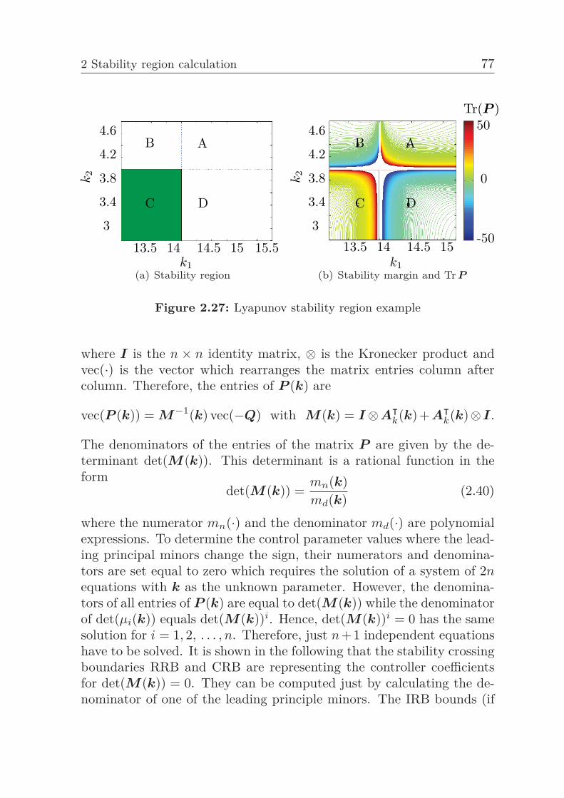
2 Stability region calculation 77
4.6
4.2
3.8
3.4
3
k2
13.5 14 14.5 15 15.5k1
B A
DC
(a) Stability region
4.6
4.2
3.8
3.4
3
k2
13.5 14 14.5 15
50
0
-50
Tr(P )
k1
B A
DC
(b) Stability margin and Tr P
Figure 2.27: Lyapunov stability region example
where I is the n × n identity matrix, ⊗ is the Kronecker product andvec(·) is the vector which rearranges the matrix entries column aftercolumn. Therefore, the entries of P (k) are
vec(P (k)) = M−1(k) vec(−Q) with M(k) = I⊗Aᵀk(k) + Aᵀ
k(k)⊗I.
The denominators of the entries of the matrix P are given by the de-terminant det(M(k)). This determinant is a rational function in theform
det(M(k)) =mn(k)md(k)
(2.40)
where the numerator mn(·) and the denominator md(·) are polynomialexpressions. To determine the control parameter values where the lead-ing principal minors change the sign, their numerators and denomina-tors are set equal to zero which requires the solution of a system of 2nequations with k as the unknown parameter. However, the denomina-tors of all entries of P (k) are equal to det(M(k)) while the denominatorof det(μi(k)) equals det(M(k))i. Hence, det(M(k))i = 0 has the samesolution for i = 1, 2, . . . , n. Therefore, just n+1 independent equationshave to be solved. It is shown in the following that the stability crossingboundaries RRB and CRB are representing the controller coefficientsfor det(M(k)) = 0. They can be computed just by calculating the de-nominator of one of the leading principle minors. The IRB bounds (if
78 2.6 Lyapunov stability-based approach
they exist) are computed from the condition det(M(k))→∞. This iscaused by the determinant of M(k) which is given in [120] as:
det(M) =n∏
i=1
n∏j=1
(λi + λj) (2.41)
where λi, . . . , λn are the eigenvalues of Ak.The RRB and the CRB cases (see figure 2.28(d) and 2.28(e)) result fromdet(M(k)) = 0 by using equation (2.41). For detM(k)) = 0, thereexists an eigenvalue λi = 0 or two imaginary eigenvalues λi and λj suchthat λi = −λj . Hence, a RRB s = 0 and CRB s = jω result if andonly if det(M(k)) = 0 holds. Since the nth principal minor of P (k)is det(P (k)) itself and det(M(k)) is the denominator of det(P (k)),det(M(k)) = 0 leads to det(P (k))→∞ which means that at least oneof the eigenvalues of P goes to infinity, see figure 2.28(a) and 2.28(b).In this case, some eigenvalues of P (k) change their signs at infinitywhile some finite eigenvalues of A(k) change their signs by crossing theimaginary axis, see figure 2.28(c) and 2.28(f). The IRB exists only ifA(k) has at least one eigenvalue at infinity, see figure 2.28(f). Equation(2.41) indicates that this happens if and only if det(M) → ∞ holds.Since det(M(k))→∞ leads to det(P (k)) = 0, at least one eigenvalueof P (k) must lie in the origin. To sum up, it is sufficient to check thefollowing two conditions:
det(M(k)) = 0, and det(M(k))→∞ (2.42)The connection between the Hurwitz criterion and the Lyapunov func-tion was studied in e.g. [182, 197, 243]. Up to now, a link between theboundary of the stability conditions has not been studied.
Remark: In order to calculate the stability boundaries, the matrix Mhas to be invertible. Accordingly, the matrix A has to be not structuralsingular. Consequently, the system should not have poles in the originwhich are independent of the uncertain parameters. However, in caseof the standard closed-loop control cycle:
G(s) =A(s)B(s)
1 + A(s)B(s)
=A(s)
B(s) + A(s)(2.43)
with a poles in the origin which is independent of the uncertain pa-rameters, the polynomial A(s) and B(s) has no coefficients which areindependent of s. Therefore, one s can be cancelled in the numerator
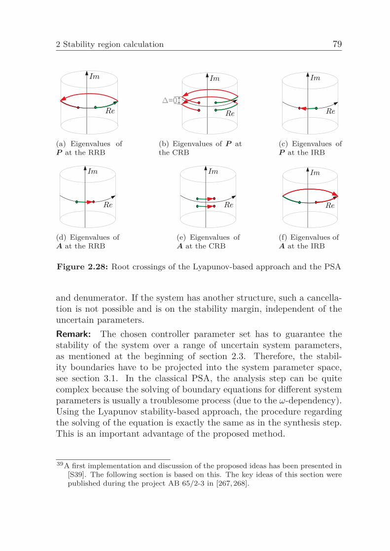
2 Stability region calculation 79
(a) Eigenvalues ofP at the RRB
(b) Eigenvalues of P atthe CRB
(c) Eigenvalues ofP at the IRB
(d) Eigenvalues ofA at the RRB
(e) Eigenvalues ofA at the CRB
(f) Eigenvalues ofA at the IRB
Figure 2.28: Root crossings of the Lyapunov-based approach and the PSA
and denumerator. If the system has another structure, such a cancella-tion is not possible and is on the stability margin, independent of theuncertain parameters.Remark: The chosen controller parameter set has to guarantee thestability of the system over a range of uncertain system parameters,as mentioned at the beginning of section 2.3. Therefore, the stabil-ity boundaries have to be projected into the system parameter space,see section 3.1. In the classical PSA, the analysis step can be quitecomplex because the solving of boundary equations for different systemparameters is usually a troublesome process (due to the ω-dependency).Using the Lyapunov stability-based approach, the procedure regardingthe solving of the equation is exactly the same as in the synthesis step.This is an important advantage of the proposed method.
39A first implementation and discussion of the proposed ideas has been presented in[S39]. The following section is based on this. The key ideas of this section werepublished during the project AB 65/2-3 in [267,268].
80 2.6 Lyapunov stability-based approach
Remark:39 In the case of the Lyapunov stability-based boundary map-ping approach, fictitious stability boundaries can occur. In some cases,entries of P are unbounded but A has no eigenvalue on the imaginaryaxis. This happens, for example, for the system δ(s,a) = s3 + a1 s2 +a2 s + a3. The Lyapunov stability study results in:
P =
⎡⎢⎢⎢⎢⎢⎢⎣−#1
#2−#3
#21
2 a3
−#3#2
−#4#2
−#5#2
12 a3
−#5#2
−#6#2
⎤⎥⎥⎥⎥⎥⎥⎦with
#1 = a1 + a3 + a2 a3
#2 = 2 a3 (a3 − a1 a2)
#3 = a12 + a1 a3 + a3
2
#4 = a13 + a1
2a3 + a1a32 + a2
2a3 + a2a3 + a3
#5 = a12 a2 + a2 a3
2 + a32
#6 = a12 a3 + a1 a2
2 + a1 a32 − a2 a3 + a3
3
For a1 = −1, a2 = −1, a3 = 1 results #2 = 0 and most entries of P areapparently infinite. However, for this case the closed-loop eigenvaluesare {−1, 1, 1}. Therefore, no eigenvalue lies on the imaginary axis. Thisshows that the approach may provide additional stability boundaries.Using the inequality property of the boundary equation set, the stableparameter space can be calculated without relying on the boundaries.Therefore, the fictitious boundaries can be ignored.
Remark: The calculation of the stabilizing kP interval can be solvedeasily with the presented method. The resulting stability boundaries arecontinuous functions in all controller parameters. Therefore, it is easyto calculate the intersection of all stability boundaries. The stabilizingkP range can be calculated by finding the minimal and maximal kP
parameters in the resulting value set.
Numerical analysis40 There are several ways how to check the defi-niteness of a matrix. The computational complexity of calculating adeterminant is O(n3) [88]. The calculation of all principal minors of an×n matrix involves the calculation of n determinants with increasingsize.
40A first implementation and discussion of the proposed ideas has been presentedin [S39, S41]. The following section is based on this.
2 Stability region calculation 81
The complexity is given by:
n∑i=1
i3 =n/2∑i=1
i3 +n∑
i=n/2
i3
The estimation of the upper and lower limit of the right sum gives:(n
4
)4≤
n∑i=n/2
(n
2
)3≤
n∑i=n/2
i3 ≤n∑
i=n/2
n3 =(
n
2
)4
Therefore, calculating all principal minors results in a computationalcomplexity of O(n4). An alternative way for testing positive definite-ness is to use the Cholesky decomposition P = LDLᵀ [88] with acomputational complexity of O(n3) [88]. In this decomposition, L is alower left and D a diagonal matrix with entries dii > 0:
xᵀP x = xᵀLDLᵀx = (Lᵀx)ᵀ DLᵀx
= yᵀDy =∑
diiy2i > 0 ∀y �= 0
(2.44)
This is equivalent to xᵀP x > 0∀x �= 0 for any regular matrix L.Hence, dii > 0, ∀i can be used for the determination of the stabilizingparameter space. The entries of dii are either zero or jump from positiveto negative infinity at the boundary.
Example 2.9. Regarding the understanding of the proposed method thecalculation of the finite boundaries (RRB and CRB) is presented in thisexample. The stabilizing parameter space is calculated for the secondorder system which was already introduced in example 2.1:
GP (s) =K
T 2s2 + 2DTs + 1,
controlled by a PID controller. The matrix Ak results in
Ak =
⎛⎜⎝ 0 1 00 0 1
−KkI
T 2 − 1+KkP
T 2 − 2DT +KkD
T 2
⎞⎟⎠
82 2.6 Lyapunov stability-based approach
with K = T = 1 and D = −0.5. Let Q = I. Therefore, det(M) resultsin the pure polynomial expression
det(M) =− 8kI(k2Dk2
P + 2k2DkP + k2
D − 2kDkIkP − 2kDkI − 2kDk2P
− 4kDkP − 2kD + k2I + 2kIkP + 2kI + k2
P + 2kP + 1)
The RRB and CRB can be calculated with det(M) = 0. In order tocompare the results the following boundaries are calculated by using thePSA: the RRB: is kI = 0 and the CRB is kP = ω2T 2 − 1/K withkI = 2dT/K + kDω2. The solution of the CRB equation set leads to theresult kI = −(1 + kP ) + (1 + kP )kD. These are the same boundarieswhich are given in the Lyapunov approach.
Example 2.10. In order to illustrate the IRB calculation, the plant
GP (s) =Ks
T 2s2 + 2DTs + 1,
controlled by a PID controller is chosen. The resulting matrix Ak
Ak =
(0 1
1+KkI
T 2+KkD
2T D+KkP
T 2+KkD
)
has a lower order in comparison to the previous example because one scan be factorized in the characteristic equation. The PSA-based stabilityboundaries are: IRB is kD = −T 2/K and RRB is kI = −K−1. ForkP = 2, K = T = 1 and D = −0.5, it follows
det(M) = − 4(kI + 1)(kD + 1)3 .
The RRB occurs in the numerator of det(M). The IRB occurs in thedenominator of det(M). This results in the same two boundaries asin the PSA, see figure 2.29(a). For a further analysis of the IRB, theeigenvalues of matrix P are calculated with kI = 1. As can be seen infigure 2.29(b) for kP = 2, kI = 1, one eigenvalue crosses the origin atthe boundary. This result is contrary to the statement of [182] in whichthe boundaries are found only in the denominator of P . Therefore, theRRB, CRB and IRB can be calculated with det(M) = 0. However, the
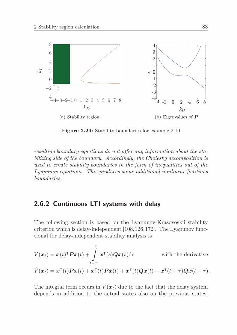
2 Stability region calculation 83
−4−3−2−1 0 1 2 3 4 5 6 7 8−4−2
02468
kD
kI
(a) Stability region (b) Eigenvalues of P
Figure 2.29: Stability boundaries for example 2.10
resulting boundary equations do not offer any information about the sta-bilizing side of the boundary. Accordingly, the Cholesky decomposition isused to create stability boundaries in the form of inequalities out of theLyapunov equations. This produces some additional nonlinear fictitiousboundaries.
2.6.2 Continuous LTI systems with delay
The following section is based on the Lyapunov-Krasovoskii stabilitycriterion which is delay-independent [108,126,172]. The Lyapunov func-tional for delay-independent stability analysis is
V (xt) = x(t)ᵀP x(t) +t∫
t−τ
xᵀ(s)Qx(s)ds with the derivative
V (xt) = xᵀ(t)P x(t) + xᵀ(t)P x(t) + xᵀ(t)Qx(t)− xᵀ(t− τ)Qx(t− τ).
The integral term occurs in V (xt) due to the fact that the delay systemdepends in addition to the actual states also on the previous states.
84 2.6 Lyapunov stability-based approach
Substituting x(t) = Ax(t) + Aτ x(t− τ) gives
V (xt) = xᵀ(t) (P A + AᵀP + Q) x(t) + xᵀ(t)P Aτ x(t− τ)+ xᵀ(t− τ)Aᵀ
τ P x(t)− xᵀ(t− τ)Qx(t− τ)
=[xᵀ(t) xᵀ(t− τ)
] [P A + AᵀP + Q P Aτ
Aᵀτ P −Q
] [x(t)
x(t− τ)
].
Similar to the delay-free case, checking the conditions V (xt) > 0 andV (xt) < 0 implies checking the definiteness of the matrices
P > 0 and S =[P A + AᵀP + Q P Aτ
Aᵀτ P −Q
]< 0⇒ Q > 0.
First order system41 Consider the first order time delay system x(t) =−ax(t) − bx(t − τ). Therefore, it results A = −q1 and Aτ = −q2. Inthis case, P and Q are scalar values. The S matrix will be
S =[−2q1P + Q −q2P−q2P −Q
]which is negative definite for
Q− 2q1P < 0 and (2.45)
−Q− q22P 2
Q− 2q1P < 0. (2.46)
The correct stability boundary results in q2 = ±q1 by using the methodsreview in section 3.1.1. Accordingly, the condition in equation (2.45)produces a fictitious stability boundary. The condition in equation(2.46) is rewritten in the form −Q2 + 2q1QP − q2
2P 2 = 0 to createthe stability boundary. The stability-critical values of the Lyapunovmatrices are chosen to P = Q = 0.0005 (which corresponds to an eigen-value next to zero). Consequently, the stability boundary results inq2 = ±√2q1 − 1. This boundary is more conservative than the oneobtained analytically as q2 = ±q1. That is due to the conservativeassumption of P and Q.
41A first implementation and discussion of the proposed ideas has been presented in[S22]. The following section is based on this. The key ideas of this section werepublished during the project AB 65/2-3 in [265].
2 Stability region calculation 85
Second order system42 Consider the following second order system:
x(t) =[
0 1−5 −2
]x(t) +
[12
]u(t)
u(t) = −kx(t) + kx(t− τ) with k = (k1,k2)
Accordingly, it yields:
A =[
−k1 1 − k2−2k1 − 5 −2k2 − 2
], Aτ =
[k1 k2
2k1 2k2
], P =
[p1,1 p1,2p2,1 p2,2
], Q =
[q1,1 q1,2q2,1 q2,2
]with q1,2 = q2,1 and p1,2 = p2,1. Unfortunately, the definiteness of theresulting S matrix now depends on both Lyapunov matrices P and Q.Then, one of the four conditions changing the definiteness of S is:
q2,2+(k1p1,2 − q1,2 + p1,1(k2 − 1) + 2p1,2(k2 + 1) + p1,2(2k1 + 5))2
2k1p1,1 − q1,1 + 2p1,2(2k1 + 5)− 2p1,2(k2 − 1)− 4p1,2(k2 + 1)= 0
The definiteness of P , Q and S changes at the boundaries of the stableregions. Next, some values of P and Q are assumed in such way thatat least one eigenvalue of each matrix equals zero, like
P =[0.0616 0.01260.0126 0.0265
]Q =
[0.126 0.1020.102 0.0822
].
The blue stability boundary in figure 2.30(a) is obtained by substitutingthese values in equation 2.6.2. Via choosing the values
P =[
0.3 0.01770.0177 0.0365
]Q =
[5.4084 0.6840.684 0.1201
]the red stability boundary in figure 2.30(a) results. Figure 2.30(b) rep-resents the correct stabilizing region. The estimated boundaries areshown in figure 2.30(a). The blue curves are corresponding to the sec-ond element which results from the Cholesky decomposition. The grayarea in figure 2.30(b) represents the resulting stability region by consid-ering all conditions resulting from the Cholesky decomposition. They42A first implementation and discussion of the proposed ideas has been presented in
[S22]. The following section is based on this. The key ideas of this section werepublished during the project AB 65/2-3 in [265].
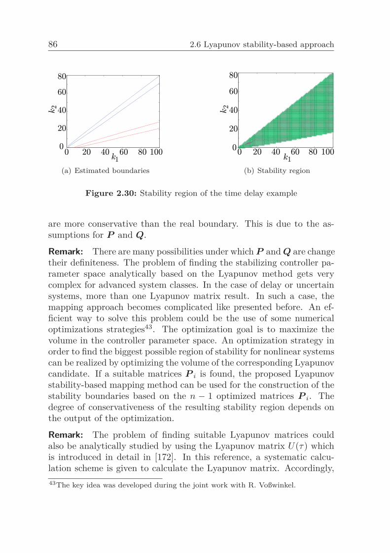
86 2.6 Lyapunov stability-based approach
(a) Estimated boundaries (b) Stability region
Figure 2.30: Stability region of the time delay example
are more conservative than the real boundary. This is due to the as-sumptions for P and Q.
Remark: There are many possibilities under which P and Q are changetheir definiteness. The problem of finding the stabilizing controller pa-rameter space analytically based on the Lyapunov method gets verycomplex for advanced system classes. In the case of delay or uncertainsystems, more than one Lyapunov matrix result. In such a case, themapping approach becomes complicated like presented before. An ef-ficient way to solve this problem could be the use of some numericaloptimizations strategies43. The optimization goal is to maximize thevolume in the controller parameter space. An optimization strategy inorder to find the biggest possible region of stability for nonlinear systemscan be realized by optimizing the volume of the corresponding Lyapunovcandidate. If a suitable matrices P i is found, the proposed Lyapunovstability-based mapping method can be used for the construction of thestability boundaries based on the n − 1 optimized matrices P i. Thedegree of conservativeness of the resulting stability region depends onthe output of the optimization.
Remark: The problem of finding suitable Lyapunov matrices couldalso be analytically studied by using the Lyapunov matrix U(τ) whichis introduced in detail in [172]. In this reference, a systematic calcu-lation scheme is given to calculate the Lyapunov matrix. Accordingly,43The key idea was developed during the joint work with R. Voßwinkel.
2 Stability region calculation 87
a randomly and therefore conservative choice of some of the entries ofthese matrices is no longer needed.
Remark: An alternative approach is could be to understand time de-lay systems as systems which can be modelled as partial differentialequations (PDEs). A method for mapping of stability boundaries ofPDE systems is presented in [249].
2.6.3 Discrete-Time LTI systems
In the following, the problem of calculating the stabilizing parameterspace for discrete-time systems is studied44. The study about discrete-time LTI systems began in the early 1960s [166]. Over the last decades,several approaches have been published, like the biquadratic transfor-mation [164] or the Tchebyshev representation [37,170]. Also the Schurstability has been analyzed by using the HBT [152]. After applyingthese transformations, principally any method for continuous systemscan be used for the boundary mapping. However, a direct way for thecalculation of the stabilizing parameter space in the discrete-time rep-resentation is preferable. This could be achieved through the approx-imation by reflection segments [25, 26]. A more exact method extendsthe PSA for the discrete-time case by using singular frequencies and alinear transformation of the parameter space [6, 28, 174]. This methodrelies on a combination of decoupling at singular frequencies, frequencysweeping and discretization of the parameter space which result in highcomputational complexity. There is also a limit to which control struc-tures may be tackled. PID controllers have been the highest order caseanalyzed in this way.The stabilizing parameter space can be computed by considering theSchur stability-based on the characteristic equation det(A(k)− zI) = 0.A system becomes stable either if an eigenvalue of A enters the unitcircle on the real axis through the point z = 1 or z = −1 or a pairof complex conjugated eigenvalues crosses the unit circle pairwise. Incontrast to continuous time systems, an IRB cannot exist because the44A first implementation and discussion of the proposed ideas has been presented in
[S41]. The following section is based on this. The key ideas of this section werepublished during the joint work with L. Pyta in [250].
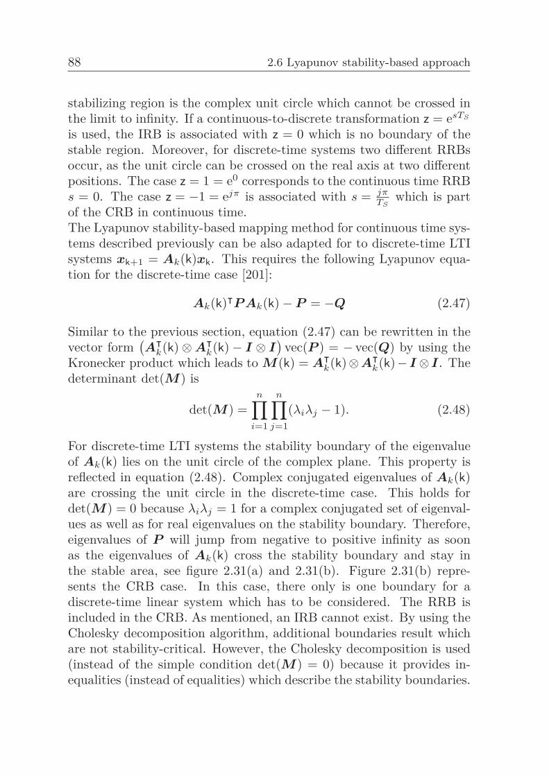
88 2.6 Lyapunov stability-based approach
stabilizing region is the complex unit circle which cannot be crossed inthe limit to infinity. If a continuous-to-discrete transformation z = esTS
is used, the IRB is associated with z = 0 which is no boundary of thestable region. Moreover, for discrete-time systems two different RRBsoccur, as the unit circle can be crossed on the real axis at two differentpositions. The case z = 1 = e0 corresponds to the continuous time RRBs = 0. The case z = −1 = ejπ is associated with s = jπ
TSwhich is part
of the CRB in continuous time.The Lyapunov stability-based mapping method for continuous time sys-tems described previously can be also adapted for to discrete-time LTIsystems xk+1 = Ak(k)xk. This requires the following Lyapunov equa-tion for the discrete-time case [201]:
Ak(k)ᵀP Ak(k)− P = −Q (2.47)
Similar to the previous section, equation (2.47) can be rewritten in thevector form
(Aᵀ
k(k)⊗Aᵀk(k)− I ⊗ I
)vec(P ) = − vec(Q) by using the
Kronecker product which leads to M(k) = Aᵀk(k)⊗Aᵀ
k(k)− I⊗ I. Thedeterminant det(M) is
det(M) =n∏
i=1
n∏j=1
(λiλj − 1). (2.48)
For discrete-time LTI systems the stability boundary of the eigenvalueof Ak(k) lies on the unit circle of the complex plane. This property isreflected in equation (2.48). Complex conjugated eigenvalues of Ak(k)are crossing the unit circle in the discrete-time case. This holds fordet(M) = 0 because λiλj = 1 for a complex conjugated set of eigenval-ues as well as for real eigenvalues on the stability boundary. Therefore,eigenvalues of P will jump from negative to positive infinity as soonas the eigenvalues of Ak(k) cross the stability boundary and stay inthe stable area, see figure 2.31(a) and 2.31(b). Figure 2.31(b) repre-sents the CRB case. In this case, there only is one boundary for adiscrete-time linear system which has to be considered. The RRB isincluded in the CRB. As mentioned, an IRB cannot exist. By using theCholesky decomposition algorithm, additional boundaries result whichare not stability-critical. However, the Cholesky decomposition is used(instead of the simple condition det(M) = 0) because it provides in-equalities (instead of equalities) which describe the stability boundaries.
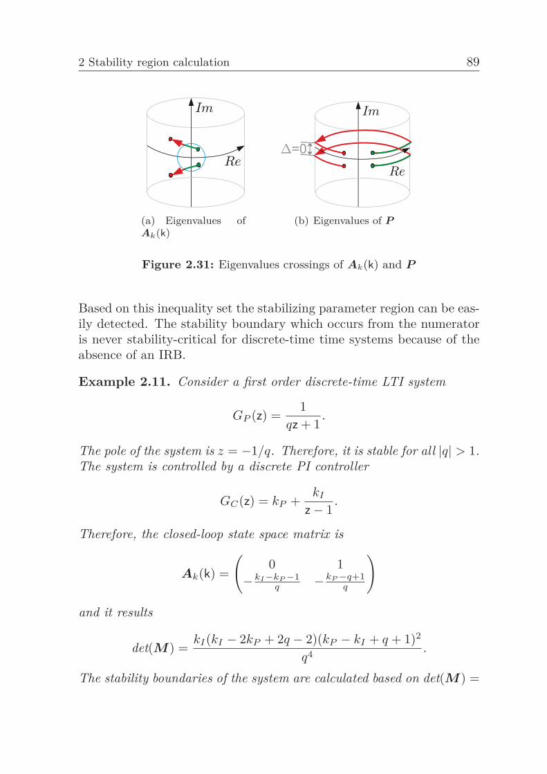
2 Stability region calculation 89
(a) Eigenvalues ofAk(k)
(b) Eigenvalues of P
Figure 2.31: Eigenvalues crossings of Ak(k) and P
Based on this inequality set the stabilizing parameter region can be eas-ily detected. The stability boundary which occurs from the numeratoris never stability-critical for discrete-time time systems because of theabsence of an IRB.
Example 2.11. Consider a first order discrete-time LTI system
GP (z) =1
qz + 1.
The pole of the system is z = −1/q. Therefore, it is stable for all |q| > 1.The system is controlled by a discrete PI controller
GC(z) = kP +kI
z− 1.
Therefore, the closed-loop state space matrix is
Ak(k) =
(0 1
−kI −kP −1q −kP −q+1
q
)
and it results
det(M) =kI(kI − 2kP + 2q − 2)(kP − kI + q + 1)2
q4 .
The stability boundaries of the system are calculated based on det(M) =
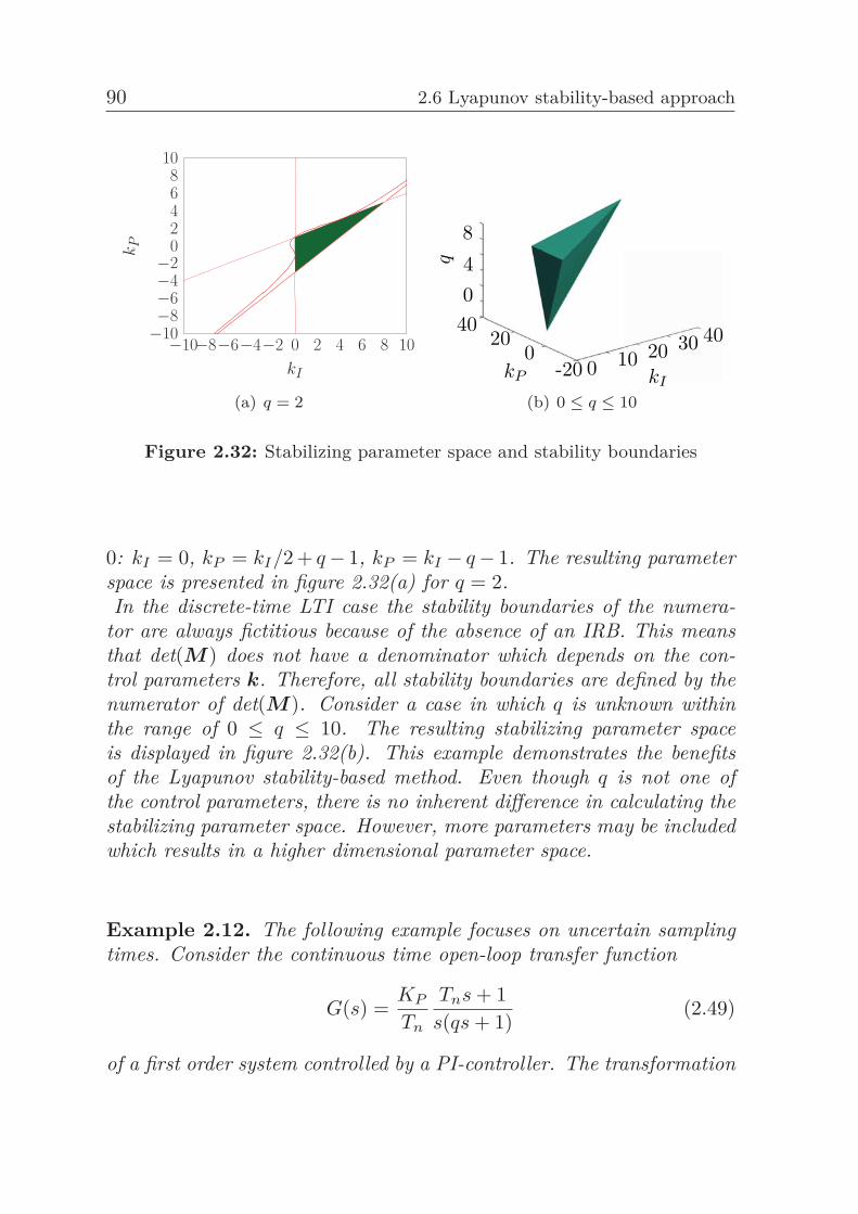
90 2.6 Lyapunov stability-based approach
−10−8−6−4−2 0 2 4 6 8 10−10−8−6−4−2
02468
10
kI
kP
(a) q = 2
840
4020
0-20 0 10 20 30 40
q
kP kI
(b) 0 ≤ q ≤ 10
Figure 2.32: Stabilizing parameter space and stability boundaries
0: kI = 0, kP = kI/2 + q− 1, kP = kI − q− 1. The resulting parameterspace is presented in figure 2.32(a) for q = 2.In the discrete-time LTI case the stability boundaries of the numera-
tor are always fictitious because of the absence of an IRB. This meansthat det(M) does not have a denominator which depends on the con-trol parameters k. Therefore, all stability boundaries are defined by thenumerator of det(M). Consider a case in which q is unknown withinthe range of 0 ≤ q ≤ 10. The resulting stabilizing parameter spaceis displayed in figure 2.32(b). This example demonstrates the benefitsof the Lyapunov stability-based method. Even though q is not one ofthe control parameters, there is no inherent difference in calculating thestabilizing parameter space. However, more parameters may be includedwhich results in a higher dimensional parameter space.
Example 2.12. The following example focuses on uncertain samplingtimes. Consider the continuous time open-loop transfer function
G(s) =KP
Tn
Tns + 1s(qs + 1)
(2.49)
of a first order system controlled by a PI-controller. The transformation
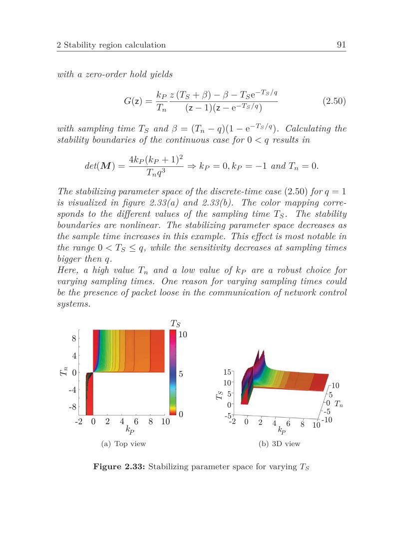
2 Stability region calculation 91
with a zero-order hold yields
G(z) =kP
Tn
z (TS + β)− β − TSe−TS/q
(z− 1)(z− e−TS/q)(2.50)
with sampling time TS and β = (Tn − q)(1 − e−TS/q). Calculating thestability boundaries of the continuous case for 0 < q results in
det(M) =4kP (kP + 1)2
Tnq3 ⇒ kP = 0, kP = −1 and Tn = 0.
The stabilizing parameter space of the discrete-time case (2.50) for q = 1is visualized in figure 2.33(a) and 2.33(b). The color mapping corre-sponds to the different values of the sampling time TS. The stabilityboundaries are nonlinear. The stabilizing parameter space decreases asthe sample time increases in this example. This effect is most notable inthe range 0 < TS ≤ q, while the sensitivity decreases at sampling timesbigger then q.Here, a high value Tn and a low value of kP are a robust choice forvarying sampling times. One reason for varying sampling times couldbe the presence of packet loose in the communication of network controlsystems.
(a) Top view (b) 3D view
Figure 2.33: Stabilizing parameter space for varying TS
92 2.6 Lyapunov stability-based approach
2.6.4 Advanced system classes
This section focuses on the stability region calculation for advancedsystem classes based on various examples. Therefore, the previous in-troduced Lyapunov stability-based mapping approach is used. The onlynecessary modification is that the Lyapunov function has to be changeddepending on the system. Accordingly, the LMI for the stability studychanges. However, the whole previous presented calculation scheme canbe applied straightforward.
Switching systems45
Switching systems are defined by a set of LTI systems x(t) = Aσx(t)with Aσ ∈ A1, . . . , AN which are switched by using the switching func-tion σ(t) : R→ {1,2,. . . }. From the stability of all single systems Aσ itcannot be concluded that the switching system is stable. One possibi-lity is to check if all eigenvalues of both convex matrix covers co(A1,A2)and co(A1,A−1
2 ) defined by co(X,Y ) = {αX + (1 − α)Y : α ∈ [0,1]}for all values of α ∈ [0,1] are in the OLHP [226]. Similarly, the switch-ing system is stable if a common quadratic Lyapunov function P existswhich fulfills the Lyapunov equation AᵀP +P A = −Q for both systemmatrices Aσ [226].
Example 2.13. Consider the example system presented in [226] withthe two system matrices
A1 =(
q1 0q2 −1
), A2 =
(0 1−1 −2
)with the convex matrix cover
co(A1,A2) =(
αq1 1 − ααq2 + α − 1 α − 2
);
co(A1,A−12 ) =
(αq1 + 2α − 2 α − 1αq2 − α + 1 −α
).
45A first implementation and discussion of the proposed ideas has been presentedin [S43]. The following section is based on this.
2 Stability region calculation 93
Therefore, the following characteristic equations result:
δ1(s,q) =s2 + (2− α(1 + q1))s + α2(1 + q1 + q2)− α(2 + 2q1 + q2) + 1δ2(s,q) =s2 + (2− α(1 + q1))s− α2(1 + q1 + q2) + αq2 + 1
For the RRB calculation results after substituting s = 0 the followingequation set:
q2 =(α2 − 2α)(q1 + 1) + 1
α− α2 =α− 21− α
q1 +α2 − 2α + 1
α− α2
q2 =α2(q1 + 1)− 1
α− α2 =α
1− αq1 +
α2 − 1α− α2
For mapping the boundaries into the q1/q2 plane, a gridding of α isneeded. A new stability boundary results or each value of α. A bound-ary with a slope of −2 results for α = 0 in the present example. Theboundary has a slope of −∞ for α→ 1.The following equation set results from the CRB substitution s = jω:
0 = −ω2 + (α2 − α) q2 + (α2 − 2α)(1 + q1) + 1 + j [2− α(1 + q1)] ω
0 = −ω2 + (α− α2) q2 − α2 (1 + q1) + 1 + j [2− α(1 + q1)] ω
Both equations have the same imaginary part
0 = [2− α(1 + q1)] ω ⇔ q1 = 2/α− 1
The following relation results for 0 ≤ α ≤ 1:
q1 ≥ 1
No CRB exists for q < 1. The substitution of the imaginary part to thereal part equations gives the following two equations:
q2 =ω2 − 2α + 3
α2 − αand q2 =
ω2 + 2α− 1α− α2
These equations representing a family of CRB boundaries which areparallel to the q1 axis for q1 ≥ 1. The stability boundaries of the switch-ing system can be analyzed by using the PSA, see the green area in
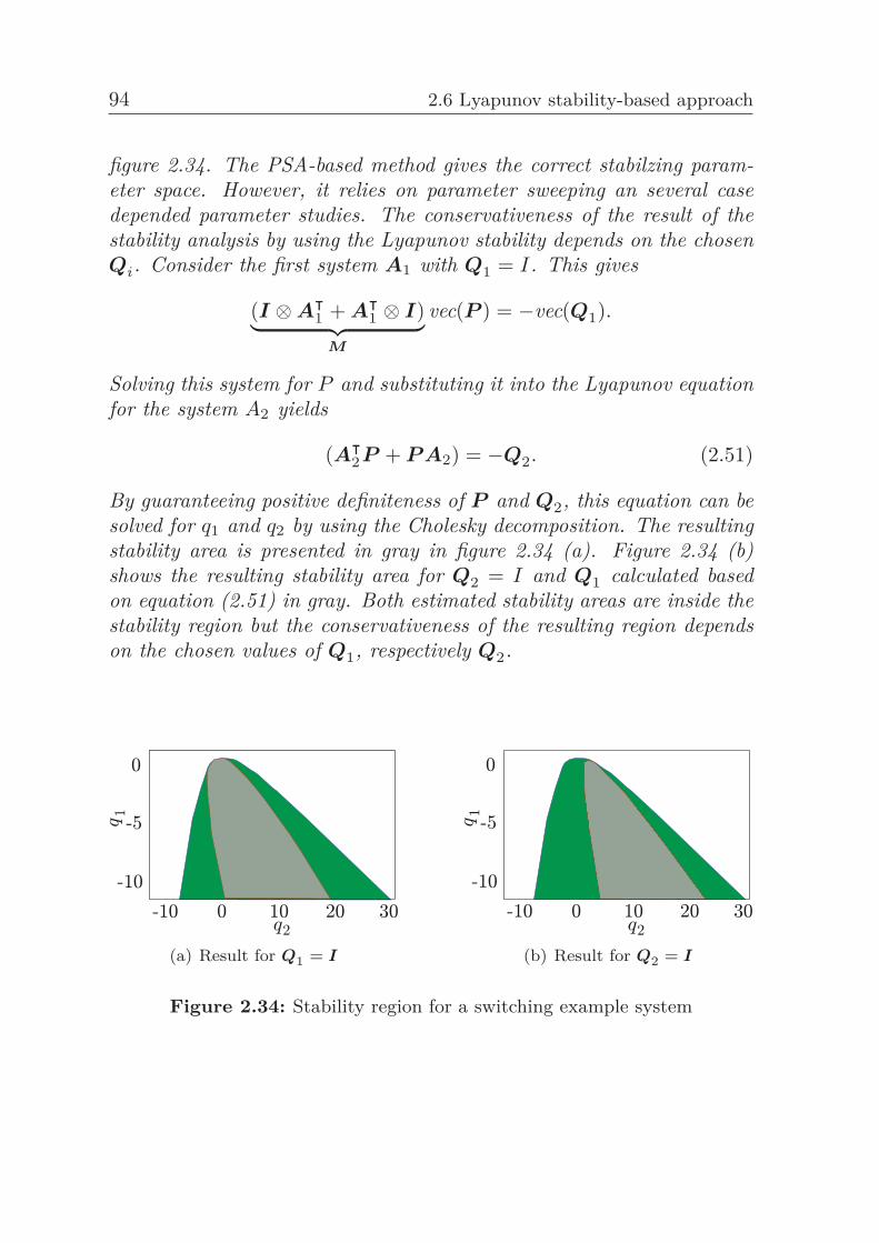
94 2.6 Lyapunov stability-based approach
figure 2.34. The PSA-based method gives the correct stabilzing param-eter space. However, it relies on parameter sweeping an several casedepended parameter studies. The conservativeness of the result of thestability analysis by using the Lyapunov stability depends on the chosenQi. Consider the first system A1 with Q1 = I. This gives
(I ⊗Aᵀ1 + Aᵀ
1 ⊗ I)︸ ︷︷ ︸M
vec(P ) = −vec(Q1).
Solving this system for P and substituting it into the Lyapunov equationfor the system A2 yields
(Aᵀ2P + P A2) = −Q2. (2.51)
By guaranteeing positive definiteness of P and Q2, this equation can besolved for q1 and q2 by using the Cholesky decomposition. The resultingstability area is presented in gray in figure 2.34 (a). Figure 2.34 (b)shows the resulting stability area for Q2 = I and Q1 calculated basedon equation (2.51) in gray. Both estimated stability areas are inside thestability region but the conservativeness of the resulting region dependson the chosen values of Q1, respectively Q2.
(a) Result for Q1 = I (b) Result for Q2 = I
Figure 2.34: Stability region for a switching example system
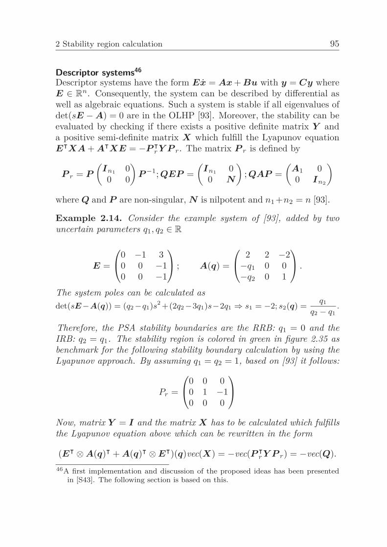
2 Stability region calculation 95
Descriptor systems46
Descriptor systems have the form Ex = Ax + Bu with y = Cy whereE ∈ R
n. Consequently, the system can be described by differential aswell as algebraic equations. Such a system is stable if all eigenvalues ofdet(sE −A) = 0 are in the OLHP [93]. Moreover, the stability can beevaluated by checking if there exists a positive definite matrix Y anda positive semi-definite matrix X which fulfill the Lyapunov equationEᵀXA + AᵀXE = −P ᵀ
r Y P r. The matrix P r is defined by
P r = P
(In1 00 0
)P −1; QEP =
(In1 00 N
); QAP =
(A1 00 In2
)where Q and P are non-singular, N is nilpotent and n1 +n2 = n [93].
Example 2.14. Consider the example system of [93], added by twouncertain parameters q1, q2 ∈ R
E =
⎛⎝0 −1 30 0 −10 0 −1
⎞⎠ ; A(q) =
⎛⎝ 2 2 −2−q1 0 0−q2 0 1
⎞⎠ .
The system poles can be calculated asdet(sE −A(q)) = (q2 −q1)s2 +(2q2 −3q1)s−2q1 ⇒ s1 = −2; s2(q) = q1
q2 − q1.
Therefore, the PSA stability boundaries are the RRB: q1 = 0 and theIRB: q2 = q1. The stability region is colored in green in figure 2.35 asbenchmark for the following stability boundary calculation by using theLyapunov approach. By assuming q1 = q2 = 1, based on [93] it follows:
Pr =
⎛⎝0 0 00 1 −10 0 0
⎞⎠Now, matrix Y = I and the matrix X has to be calculated which fulfillsthe Lyapunov equation above which can be rewritten in the form
(Eᵀ ⊗A(q)ᵀ + A(q)ᵀ ⊗Eᵀ)(q)vec(X) = −vec(P ᵀr Y P r) = −vec(Q).
46A first implementation and discussion of the proposed ideas has been presentedin [S43]. The following section is based on this.
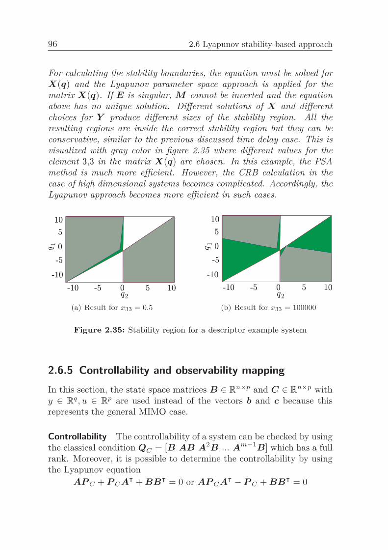
96 2.6 Lyapunov stability-based approach
For calculating the stability boundaries, the equation must be solved forX(q) and the Lyapunov parameter space approach is applied for thematrix X(q). If E is singular, M cannot be inverted and the equationabove has no unique solution. Different solutions of X and differentchoices for Y produce different sizes of the stability region. All theresulting regions are inside the correct stability region but they can beconservative, similar to the previous discussed time delay case. This isvisualized with gray color in figure 2.35 where different values for theelement 3,3 in the matrix X(q) are chosen. In this example, the PSAmethod is much more efficient. However, the CRB calculation in thecase of high dimensional systems becomes complicated. Accordingly, theLyapunov approach becomes more efficient in such cases.
(a) Result for x33 = 0.5 (b) Result for x33 = 100000
Figure 2.35: Stability region for a descriptor example system
2.6.5 Controllability and observability mappingIn this section, the state space matrices B ∈ R
n×p and C ∈ Rn×p with
y ∈ Rq, u ∈ R
p are used instead of the vectors b and c because thisrepresents the general MIMO case.
Controllability The controllability of a system can be checked by usingthe classical condition QC = [B AB A2B ... Am−1B] which has a fullrank. Moreover, it is possible to determine the controllability by usingthe Lyapunov equation
AP C + P CAᵀ + BBᵀ = 0 or AP CAᵀ − P C + BBᵀ = 0
2 Stability region calculation 97
with the solution
P C =∞∫
0
eAtBBᵀeAtdt and P C =∞∑
k=0AkBBᵀ(Aᵀ)k
for the continuous as well as for the discrete-time case which is namedcontrollability gramian [193].
Observability A similar procedure is applicable for the observabilitytest. The condition Q0 = [C CA CA2 ... CAm−1]ᵀ which has a fullrank can be used. In addition, the Lyapunov equation
AᵀP O + P OA + CᵀC = 0 or AᵀP CA− P O + CᵀC = 0can be utilized with the solution
P O =∞∫
0
eAtCᵀCeAtdt and P O =∞∑
k=0(Aᵀ)kCᵀCAk
for the continuous as well as for the discrete-time case which is namedobservability gramian [193].
Mapping The previously introduced controllability and observabilitygramian can be used to map the controllability and observability prop-erty of a system to the parameter space. This can be done by using theLyapunov mapping method. Similar, the matrices QC and QO couldalso be used for the mapping. From a practical point of view, such amapping could be utilized to analyze the effect of sensor or actor lossesto a systems.
2.7 Probabilistic-based approachSeveral probabilistic approaches for robust controller design do exist inthe literature. They deal with probabilistic relaxations and randomizeduncertainties by using e.g. Monte Carlo methods. These approacheswill be extended in the following for the calculation of the stability re-gions. The philosophy of these approaches is quite different from themethods which will be presented in section 3. The approaches don’t tryto find parameters which will stabilize the system under considerationof all worst case combinations of the uncertain parameters. Instead,they try to find parameter sets which stabilize a system with a spec-ified probability under explicit consideration of the probability of the
98 2.7 Probabilistic-based approach
parameter uncertainties. This leads to less conservative performancebut cannot guaranty closed-loop stability over the whole operating do-main Q. For more details about the theory of probabilistic approachesfor robust controller design, see [67, 312]. Recent tools for this field ofresearch has been presented in [69]. A probabilistic approach47 for cal-culating the stabilizing parameter region is briefly illustrated next. Inthis approach, an adaptive support vector machine (SVM) algorithm isused to cluster sampling points inside the parameter region into stableand unstable regions. The basic idea of SVMs is to find an optimalseparating hyperplane to cluster two sets of candidate points, see fig-ure 2.36(a). The optimization goal is to find a separating hyperplane(black line) which has a maximum distance Δ to the nearest neigh-boring candidate points. In this case, the parameter space consists ofthe two controller parameters k1 and k2. The stable candidate pointsare denoted by blue rectangles and the unstable by red circles. Theseparating hyperplane results in an analytical expression as a functionof the parameters of interest. The optimization problem can be for-mulated as a quadratic optimization problem. Several modifications ofthe classical SVM idea are known, like the famous kernel trick to cal-culate nonlinear separating hyperplanes. A detailed introduction aboutSVMs is given in [58]. The developed method works as follows. Thefirst step for the stability region calculation is to spread a small numberof points inside the parameter space by using the design of experimentmethods. Actual, a latinized centroidal voronoi tesellation distributionis chosen which is a very uniform distribution. Thereafter, a stabilitycheck for each point has to be applied. This depends on the system classof interest. The stability test in the LTI case is an eigenvalue calcula-tion. Also the describing functions can be used to check the stabilityof more advanced system classes. Next, the SVM algorithm calculatesthe optimal separating hyperplane to clusters the parameter space intostability and instability regions. To increase the computation efficiency,an adaptive sampling algorithm is used. This algorithm spreads pointsnext to the previously calculated separating hyperplane to increase thecalculation accuracy iteratively until a predefined precision is reached.This method has an efficient learning ability, it can deal with multi-47A first implementation and discussion of the proposed ideas has been presented
in [S10, S13, S38]. The following section is based on this. The key ideas of thissection were developed during the joint work with H. Arenbeck
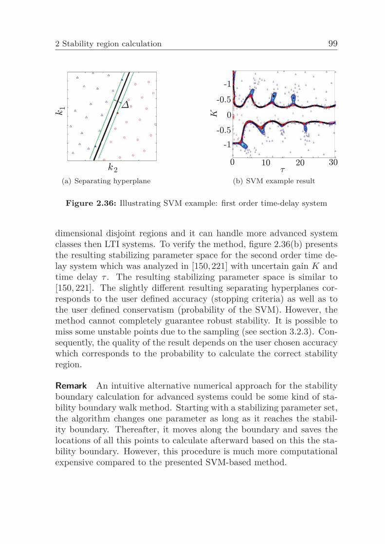
2 Stability region calculation 99
(a) Separating hyperplane (b) SVM example result
Figure 2.36: Illustrating SVM example: first order time-delay system
dimensional disjoint regions and it can handle more advanced systemclasses then LTI systems. To verify the method, figure 2.36(b) presentsthe resulting stabilizing parameter space for the second order time de-lay system which was analyzed in [150,221] with uncertain gain K andtime delay τ . The resulting stabilizing parameter space is similar to[150, 221]. The slightly different resulting separating hyperplanes cor-responds to the user defined accuracy (stopping criteria) as well as tothe user defined conservatism (probability of the SVM). However, themethod cannot completely guarantee robust stability. It is possible tomiss some unstable points due to the sampling (see section 3.2.3). Con-sequently, the quality of the result depends on the user chosen accuracywhich corresponds to the probability to calculate the correct stabilityregion.
Remark An intuitive alternative numerical approach for the stabilityboundary calculation for advanced systems could be some kind of sta-bility boundary walk method. Starting with a stabilizing parameter set,the algorithm changes one parameter as long as it reaches the stabil-ity boundary. Thereafter, it moves along the boundary and saves thelocations of all this points to calculate afterward based on this the sta-bility boundary. However, this procedure is much more computationalexpensive compared to the presented SVM-based method.
100
3 Robustness-based synthesisControl theory has gained significant progress regarding analysis andsynthesis methods for the control of linear systems over the past decades.A mandatory requirement for the application of these methods is a lin-ear mathematical model of the controlled system. In practice, it isnearly impossible to describe the dynamic behavior of a real systemcompletely by use of a linear model. Hence, the models have errors dueto dynamic simplification, linearization and measurement errors. Asmentioned in the beginning of this dissertation robust control offers away to handle such model errors. A simple design method which is gen-erally applicable for a system with any parameter uncertainties is stillan open question in research [142]. Recent solutions are e.g. based onH∞ [115], IQC [358] or interval arithmetic [195]. These approaches areoften conservative and produce a high computational effort. The mainfocus of the following section is the development of techniques for thedesign of a time-invariant controller in order to stabilize a given systemunder consideration of the time-invariant uncertain model parameters.There is a trade-off between robustness and performance. It is desirableto have a system with both: high performance and strong robustness.Therefore, a compromise between both must be reached through con-troller design. Based on this, a robust system with an additional largestability margin is considered as a drawback because it indicates poorperformance. Therefore, the controller design goal is to find tight ro-bustness that is able to keep the system stable against specified uncer-tainties with desirable performance specifications during nominal con-ditions [320].Consequently, methods for the expansion of the analysis step of thePSA to more general system classes are studied (section 3.1). There-after, the PSA will be simplified to a one step procedure to overcome theanalysis step for some special system classes (section 3.2). This highlyimproves the usability and efficiency of the PSA. Next, some results forLTV systems will be developed (section 3.3) and graphical verificationtechniques for robust controller design will be reviewed (section 3.4).
3 Robustness-based synthesis 101
3.1 Analysis stepThis section focuses on the development of a systematical calculationprocedure for the analysis step of the PSA. In the classical PSA, theanalysis step is necessary to ensure that the chosen controller parametersare robustly stable for the whole system parameter family δ(s,Q,K) ={δ(s, k, q) | q ∈ Q ∧ k ∈ K}, see [4]. Therefore, the controller parame-ters have to be mapped into the system parameter space and it needsto be checked if Q is completely inside the stabilizing system parameterspace. If this condition is not fulfilled, the controller parameters have tobe modified iteratively. Consequently, also this step is based on stabil-ity boundary calculations. The RRB can be easily calculated based onδ(s = 0, k, q) = 0. Accordingly, an easy boundary condition results. Inthe case of a single-loop PID controlled system, a RRB does not exist inthe synthesis step because the previously mentioned substitution yieldsa0 kI + b0 = 0 ⇒ a0 kI = 0. Hence, the RRB is independent of plantparameters. The IRB calculation works similar: δ(s → ∞, k, q) = 0.Depending on the control structure, this can lead to a lengthy casestudy similar to section 2.3.3. The calculation of the CRB boundary ismore complicated. The boundary equations are depending on the sys-tem order and the system parameters of interest. Consequently, an easydecoupling strategy of the CRB equations like in the synthesis step can-not be applied to create the CRBs. Therefore, the CRB calculation fordifferent cases is discussed next. In the following subsection, methodsare explained which consider uncertainties in the delay. Afterwards, thecontroller gains as well as the value of the time delay are assumed to beconstant and all other system parameters are uncertain. Thereafter insection 3.1.3 several ideas to handle more advanced system classes aredemonstrated.
3.1.1 Delay parameter region chartsMethods will be discussed which consider uncertainties in the delay. Anotation similar to [206] will be used. Consider the delay differentialequation in the form
∂
∂t
⎛⎝x(t) +o∑
i=1F ix(t− τk)
⎞⎠ = Ax(t) +o∑
i=1Aτ,ix(t− τi) (3.1)
102 3.1 Analysis step
with the system matrices A, Aτ,1 ... Aτ,o ∈ Nn×n and the states x(t) ∈
Rn at the time instant t. The variables 0 < τ1 < τ2 ... < τo denote the
different delays. The type matrices F 1, F 2 ... F o ∈ Nn×n are defining
the type of the delay differential equation. A retarded system resultsfor example if F i = 0 holds ∀F i. The eigenvalues of the system can becalculated based on det(δ(s)) = 0 with
δ(s) := s
⎛⎝I −o∑
i=1F ixe−sτi
⎞⎠−A−o∑
i=1Aie−sτi . (3.2)
In the following, a brief overview of the most popular calculation meth-ods to draw the delay parameter region will be presented. Much re-search was conducted by different research groups, as presented next.Unfortunately, so far there is no clear connection between the differentapproaches. Therefore, the following section focuses on the generaliza-tion of the available approaches in order to point out where the originand the connection between the different approaches is.All methods that will be discussed next are based on the continuitytheorem [80] which states that if the system is stable for some valuesof certain parameters and unstable for other values, there must be avalue in between where the system is on the stability margin (poles onthe imaginary axis), similar to section 2.2. More in detail, the delayspace methods are based on the τ -decomposition concept [206] whichdivides the delay axis into intervals where each interval consists of thesame number of unstable roots NU(τ). A time delay system which haspoles on the imaginary axis satisfies equation (3.2) for s = jωτ withthe crossing frequency ωτ ∈ �+. The value τ = ττi that satisfies thecharacteristic equation for s = ωτ is called the crossing delay. Thisutilizes the cluster treatment of characteristic roots (CTCR) paradigm[222] which states that the set of all crossing frequencies consists of notmore than n2 elements where n is the system order. For each cross-ing frequency there is a cluster of infinite number of crossing delaysττi = τc + 2πi/ωτ with i = 0, 1, 2, . . . that satisfies equation (3.2) whereττ is the smallest possible value of delay that satisfies equation (3.2) fors = jωτ . The period between two crossing delays in the same cluster is2π/ωτ . The period is smaller and the crossing rate is higher for highercrossing frequencies, see discussions about the root chains in section 2.1.
3 Robustness-based synthesis 103
An additional property for CTCR is the root tendency (RT) invarianceproperty which describes the behavior of the poles on the imaginaryaxis after a small disturbance ε. The RT is defined by
RT = sign[Re
(∂s/∂τ |s=jωτ τ=τc+ε
)]. (3.3)
The RT is the same for all crossing delays in one cluster (ωτ ,ττi) [232].The cluster (ωτ ,ττi) is destabilizing for RT = 1 and the poles are crossingfrom the OLHP to the ORHP. The cluster is stabilizing for RT = −1and the poles are crossing from the ORHP to the OLHP. The followinglist summarizes the procedure for each delay space method:
1. Determine whether the system is stabilizable or not (e.g. use theroot chains). If the system is stabilizable, proceed to the nextstep.
2. Substitute τ = 0 in equation (3.2) and calculate NU(0) (e.g. useRouth-Hurwitz). If NU(0) is odd, the system cannot be stable forany value of τ , due to the geometry of the root chains (complexconjugate pole pairs).
3. Calculate the clusters {ωτ , ττi} by using any of the following pre-sented delay space methods and calculate the RT of each cluster.
4. Sort the set {ττi} in ascending order and calculate NU for eachinterval by using the RT of each ττi. NU = 0 indicates stabledelay intervals.
Direct method This intuitive and straightforward approach was intro-duced in [77, 328]. The characteristic equation for linear systems withsingle unknown delay has the form δ(jω, τ) = B(jω) + A(jω)e−sτ = 0.A necessary and sufficient condition for calculating values of τ whichlead to roots on the imaginary axis is that s = jω is the solution ofthe characteristic equation. The substitution s = −jω also satisfiesthe characteristic equation δ(−jω, τ) = B(−jω) + A(−jω)e jωτ = 0 dueto the fact that the roots always cross the imaginary axis with com-plex conjugated pole pairs. Equalizing both equations give W (ω) =B(jω)B(−jω) − A(jω)A(−jω) = 0 which is a finite dimension polyno-mial in ω with degree n2 and independent of τ . A similar idea wasproposed in section 2.4 for the HBT. The equation W (ω) = 0 has tobe solved for ω. If ωτ is sorted in descending order, the first crossing
104 3.1 Analysis step
frequency is destabilizing, the second stabilizing and so on [328]. Thisproperty can be used instead of calculating the RT. The solution for theassociated ττi values with each ωτ can be obtained by using real andimaginary part of the characteristic equation
cos(ωτ τ) = �(−B(jωτ )
A(jωτ )
)and sin(ωτ τ) = �
(B(jωτ )A(jωτ )
).
Solving for τ yields to
ττk = tan−1(�(B(jωτ )/A(jωτ ))�(−B(jωτ )/A(jωτ ))
)+
2πk
ωτk = 0,1,2, . . . . (3.4)
If there are no real solutions for W (ω), there will be no crossing as τincreases and the system will be stable/unstable independent of delay.The basic idea of decoupling the characteristic equation to a delay-dependent and a delay independent equation can be traced back to Y.Z. Tsypkin [316] as well as the first delay root locus studies. In thisapproaches, the magnitude and phase condition were studied to findthe stabilizing time delay intervals. Therefore, the W (ω) function isreplaced by the gain condition. N. Hohenbichler presented an extensionof the direct method in [148]. His approach can be used to show amixed region of the delay and system parameters. However, this is onlyapplicable for special systems and delay parameter combinations due tothe coupling of magnitude and phase condition. The direct method canbe extended for two delays [328] but fictitious crossing frequencies willoccur [296].
Rekasius method This method was firstly introduced in [95] and uti-lized in [222,232,233,313]. By using the substitution
e−τs =1− Ts
1 + Ts, T ∈ R, τ ∈ R
+ (3.5)the infinite dimension quasi-polynomial in equation (3.2) is transformedinto a finite dimensional polynomial
δ(s,T ) =n∑
i=0ai(s)(1 + Ts)n−i(1− Ts)i = 0 (3.6)
of order n2. This substitution only holds for crossing frequencies whenthe original system has poles on the imaginary axis. The values Tτ thatcause poles on the imaginary axis have to be calculated by creating the
3 Robustness-based synthesis 105
Routh-Hurwitz array of equation (3.6). According to [222] it is onlyrequired to solve the entry R11(T ) in the Routh-Hurwitz table for realvalues of T and to substitute these values in the two terms R21(T )and R22(T ). If the two terms have the same sign, then these valuesof T should be included in {Tτ}. The crossing frequencies are given byωτ =
√R22/R21 which maps Tτ to ωτ . The values of ττk can be derived
by equating the phases in equation (3.5):
ττk =2
ωτ[tan−1(ωτ Tτ ) + kπ] k = 0,1,2, . . . (3.7)
Similar to the direct method, this approach is also based on findingthe stability margin pairs of ωτ /ττ . The calculation complexity of thisapproach increases strongly for high order systems. The expansion forthe two delay cases is given e.g. in [295].
Matrix multiplication method This method was introduced in [190]and follows a similar idea like the direct method. It eliminates thedelay dependency and solves the resulting equation for the crossingfrequencies. The characteristic equation in the form
δ(s,τ) = det(sI −A + (−sF 1 −A1)e−τs) = 0 (3.8)
can be transformed to the eigenvalue problem (sI−A)v = e−τs(sF 1 +A1)v with v �= 0. Conjugating and transposing this, it gives v∗(sI +Aᵀ) = e τsv∗(sF ᵀ
1 −Aᵀ1). Multiplying both equations with each other
eliminates the delay term and gives (sI − A)vv∗(sI + Aᵀ) = (sF 1 +A1)vv∗(sF ᵀ
1 − Aᵀ1). This can be written as ((sI − A) ⊗ (sI + A) −
(sF 1 + A1) ⊗ (sF 1 −A1))u = 0 where u = ξvv∗. This equation canbe interpreted as an eigenvalue problem of det(sE − J) = 0 where
E =[
I ⊗ I F 1 ⊗ II ⊗ F 1 I ⊗ I
]and J =
[A⊗ I −A1 ⊗ II ⊗A1 −I ⊗A
].
The crossing frequency set {ωτ} of equation (3.8) can be calculated bycomputing the purely imaginary generalized eigenvalues of the matrixpair (J,E) [62, 121]. The modified Schur-Cohen method and the ma-trix sum method developed by J. Chen [161] are working very similar.These two methods are also based on computing generalized eigenvalues
106 3.1 Analysis step
of a certain constant matrix pencil as well as eigenvalues of a certainconstant matrix. Similar to equation (3.4), the delay ττk is given by
ττk = (−∠z + 2πk)/ωτ k = 0,1,2, . . . . (3.9)
An extension of this method to multi delays is demonstrated in [306].
Remark: Since the first methods to deal with two delay systems wereproposed in [136], several additional approaches were developed. Theinterested reader can find an geometric approach which offers a detailedstudy of the shapes of the resulting stability graphs in [129]. The ex-pansion for three delays is explained in [127].
All the presented methods in section 3.2.1 are based on the calculationof the value pairs ωτ /ττ . The methods are using different algebraiccalculation schemes, but the computation effort is nearly the same forall methods. The parameter space method doesn’t seem to expand thesemethods. Therefore, the problem of creating system parameter regioncharts for fixed delays is studied next.
3.1.2 System parameter region chartsRegarding the previous methods, the crossing frequencies were not de-pendent on other system parameters. Thus, for each crossing frequencya cluster of crossing delays results. The problem becomes complicatedwhen other system parameters are uncertain and the delay is fixed.In this case, the crossing frequencies change when the parameters arechanging. All of the previous methods fail in solving this problem. Onlya few sketched solutions are available for this problem. For example,C. S. Hsu and S. J. Bhatt have drawn stability charts for second ordersystems [154]. Also G. Stepan has provided a number of stability chartsfor low order systems [303]. There is also a semi-discretization methodto draw stable regions in system parameter spaces in [160]. However,a systematically procedure to draw stability region charts for systemparameters is lacking. Therefore, the PSA will be extended to mapstability regions in system parameter space.
Single-loop PID controlled first order delay-free system Considerthe system GP (s, q) = a0 / (b1 s + b0). The characteristic function isδ (s, q k) =
(kI + kP s + kD s2) a0 + s(b1 s + b0) . The CRB equation
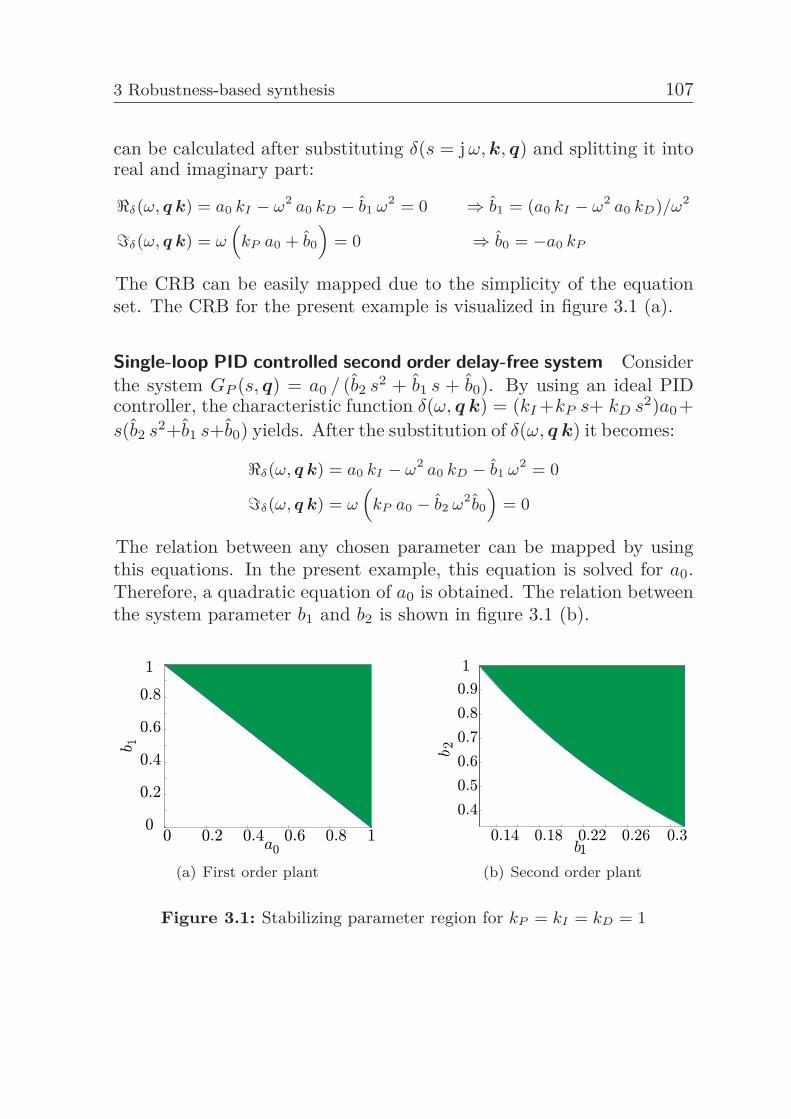
3 Robustness-based synthesis 107
can be calculated after substituting δ(s = j ω, k, q) and splitting it intoreal and imaginary part:
�δ(ω, q k) = a0 kI − ω2 a0 kD − b1 ω2 = 0 ⇒ b1 = (a0 kI − ω2 a0 kD)/ω2
�δ(ω, q k) = ω(
kP a0 + b0
)= 0 ⇒ b0 = −a0 kP
The CRB can be easily mapped due to the simplicity of the equationset. The CRB for the present example is visualized in figure 3.1 (a).
Single-loop PID controlled second order delay-free system Considerthe system GP (s, q) = a0 / (b2 s2 + b1 s + b0). By using an ideal PIDcontroller, the characteristic function δ(ω, q k) = (kI +kP s+ kD s2)a0+s(b2 s2+b1 s+b0) yields. After the substitution of δ(ω, q k) it becomes:
�δ(ω, q k) = a0 kI − ω2 a0 kD − b1 ω2 = 0
�δ(ω, q k) = ω(
kP a0 − b2 ω2b0
)= 0
The relation between any chosen parameter can be mapped by usingthis equations. In the present example, this equation is solved for a0.Therefore, a quadratic equation of a0 is obtained. The relation betweenthe system parameter b1 and b2 is shown in figure 3.1 (b).
(a) First order plant (b) Second order plant
Figure 3.1: Stabilizing parameter region for kP = kI = kD = 1
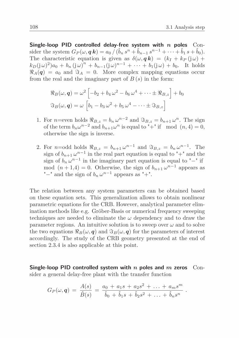
108 3.1 Analysis step
Single-loop PID controlled delay-free system with n poles Con-sider the system GP (ω, q k) = a0 / (bn sn + bn−1 sn−1 + · · ·+ b1 s + b0).The characteristic equation is given as δ(ω, q k) = (kI + kP (j ω) +kD(j ω)2)a0 + bn (j ω)n + bn−1(j ω)n−1 + · · · + b1(j ω) + b0. It holds�A(q) = a0 and �A = 0. More complex mapping equations occurfrom the real and the imaginary part of B (s) in the form:
�B(ω, q) = ω2[−b2 + b4 ω2 − b6 ω4 + · · · ± �B,z
]+ b0
�B(ω, q) = ω[b1 − b3 ω2 + b5 ω4 − · · · ± �B,z
]1. For n=even holds �B,z = bn ωn−2 and �B,z = bn+1 ωn. The sign
of the term bnωn−2 and bn+1ωn is equal to "+" if mod (n, 4) = 0,otherwise the sign is inverse.
2. For n=odd holds �B,z = bn+1 ωn−1 and �B,z = bn ωn−1. Thesign of bn+1 ωn−1 in the real part equation is equal to "+" and thesign of bn ωn−1 in the imaginary part equation is equal to "−" ifmod (n + 1,4) = 0. Otherwise, the sign of bn+1 ωn−1 appears as"−" and the sign of bn ωn−1 appears as "+".
The relation between any system parameters can be obtained basedon these equation sets. This generalization allows to obtain nonlinearparametric equations for the CRB. However, analytical parameter elim-ination methods like e.g. Gröber-Basis or numerical frequency sweepingtechniques are needed to eliminate the ω dependency and to draw theparameter regions. An intuitive solution is to sweep over ω and to solvethe two equations �B(ω, q) and �B(ω, q) for the parameters of interestaccordingly. The study of the CRB geometry presented at the end ofsection 2.3.4 is also applicable at this point.
Single-loop PID controlled system with n poles and m zeros Con-sider a general delay-free plant with the transfer function
GP (ω, q) =A(s)B(s)
=a0 + a1s + a2s2 + . . . + amsm
b0 + b1s + b2s2 + . . . + bnsn.
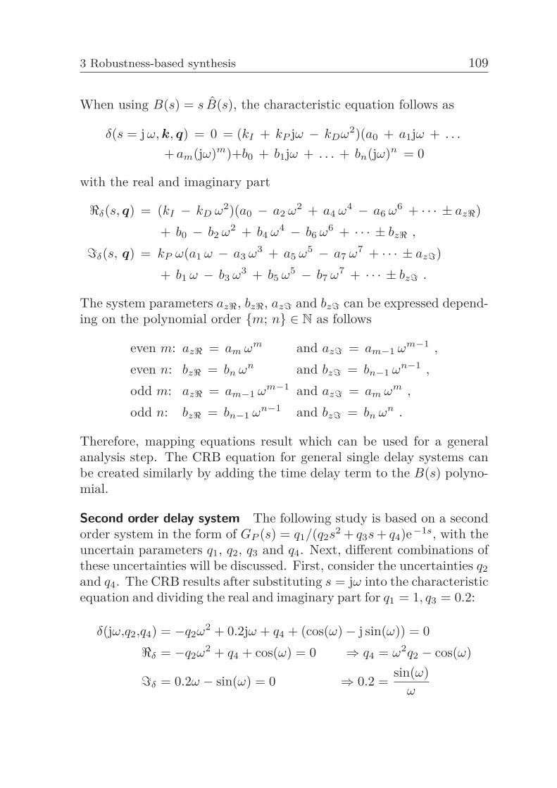
3 Robustness-based synthesis 109
When using B(s) = s B(s), the characteristic equation follows as
δ(s = j ω, k, q) = 0 = (kI + kP jω − kDω2)(a0 + a1jω + . . .
+ am(jω)m)+b0 + b1jω + . . . + bn(jω)n = 0
with the real and imaginary part
�δ(s, q) = (kI − kD ω2)(a0 − a2 ω2 + a4 ω4 − a6 ω6 + · · · ± az�)+ b0 − b2 ω2 + b4 ω4 − b6 ω6 + · · · ± bz� ,
�δ(s, q) = kP ω(a1 ω − a3 ω3 + a5 ω5 − a7 ω7 + · · · ± az�)+ b1 ω − b3 ω3 + b5 ω5 − b7 ω7 + · · · ± bz� .
The system parameters az�, bz�, az� and bz� can be expressed depend-ing on the polynomial order {m; n} ∈ N as follows
even m: az� = am ωm and az� = am−1 ωm−1 ,
even n: bz� = bn ωn and bz� = bn−1 ωn−1 ,
odd m: az� = am−1 ωm−1 and az� = am ωm ,
odd n: bz� = bn−1 ωn−1 and bz� = bn ωn .
Therefore, mapping equations result which can be used for a generalanalysis step. The CRB equation for general single delay systems canbe created similarly by adding the time delay term to the B(s) polyno-mial.
Second order delay system The following study is based on a secondorder system in the form of GP (s) = q1/(q2s2 + q3s + q4)e−1s, with theuncertain parameters q1, q2, q3 and q4. Next, different combinations ofthese uncertainties will be discussed. First, consider the uncertainties q2and q4. The CRB results after substituting s = jω into the characteristicequation and dividing the real and imaginary part for q1 = 1, q3 = 0.2:
δ(jω,q2,q4) = −q2ω2 + 0.2jω + q4 + (cos(ω)− j sin(ω)) = 0�δ = −q2ω2 + q4 + cos(ω) = 0 ⇒ q4 = ω2q2 − cos(ω)
�δ = 0.2ω − sin(ω) = 0 ⇒ 0.2 =sin(ω)
ω
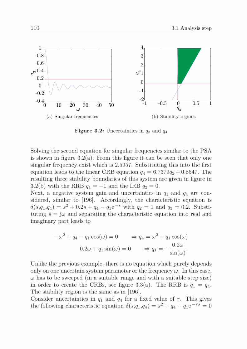
110 3.1 Analysis step
(a) Singular frequencies (b) Stability regions
Figure 3.2: Uncertainties in q2 and q4
Solving the second equation for singular frequencies similar to the PSAis shown in figure 3.2(a). From this figure it can be seen that only onesingular frequency exist which is 2.5957. Substituting this into the firstequation leads to the linear CRB equation q4 = 6.7379q2 + 0.8547. Theresulting three stability boundaries of this system are given in figure in3.2(b) with the RRB q1 = −1 and the IRB q2 = 0.Next, a negative system gain and uncertainties in q1 and q4 are con-sidered, similar to [196]. Accordingly, the characteristic equation isδ(s,q1,q4) = s2 + 0.2s + q4 − q1e−s with q2 = 1 and q3 = 0.2. Substi-tuting s = jω and separating the characteristic equation into real andimaginary part leads to
−ω2 + q4 − q1 cos(ω) = 0 ⇒ q4 = ω2 + q1 cos(ω)
0.2ω + q1 sin(ω) = 0 ⇒ q1 = − 0.2ω
sin(ω).
Unlike the previous example, there is no equation which purely dependsonly on one uncertain system parameter or the frequency ω. In this case,ω has to be sweeped (in a suitable range and with a suitable step size)in order to create the CRBs, see figure 3.3(a). The RRB is q1 = q4.The stability region is the same as in [196].Consider uncertainties in q1 and q4 for a fixed value of τ . This givesthe following characteristic equation δ(s,q1,q4) = s2 + q4 − q1e−τs = 0
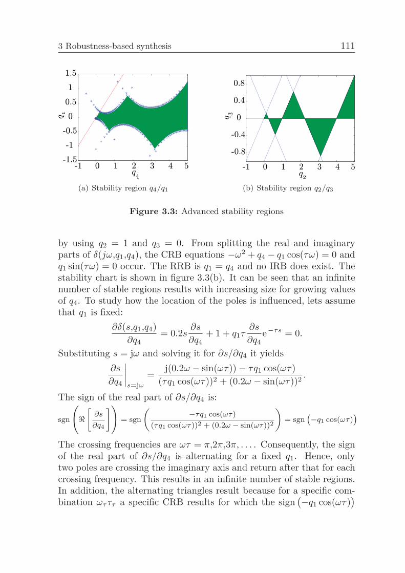
3 Robustness-based synthesis 111
(a) Stability region q4/q1 (b) Stability region q2/q3
Figure 3.3: Advanced stability regions
by using q2 = 1 and q3 = 0. From splitting the real and imaginaryparts of δ(jω,q1,q4), the CRB equations −ω2 + q4 − q1 cos(τω) = 0 andq1 sin(τω) = 0 occur. The RRB is q1 = q4 and no IRB does exist. Thestability chart is shown in figure 3.3(b). It can be seen that an infinitenumber of stable regions results with increasing size for growing valuesof q4. To study how the location of the poles is influenced, lets assumethat q1 is fixed:
∂δ(s,q1,q4)∂q4
= 0.2s∂s
∂q4+ 1 + q1τ
∂s
∂q4e−τs = 0.
Substituting s = jω and solving it for ∂s/∂q4 it yields∂s
∂q4
∣∣∣∣s=jω
=j(0.2ω − sin(ωτ))− τq1 cos(ωτ)
(τq1 cos(ωτ))2 + (0.2ω − sin(ωτ))2 .
The sign of the real part of ∂s/∂q4 is:
sgn
(�[
∂s
∂q4
])= sgn
(−τq1 cos(ωτ)
(τq1 cos(ωτ))2 + (0.2ω − sin(ωτ))2
)= sgn
(−q1 cos(ωτ)
)The crossing frequencies are ωτ = π,2π,3π, . . . . Consequently, the signof the real part of ∂s/∂q4 is alternating for a fixed q1. Hence, onlytwo poles are crossing the imaginary axis and return after that for eachcrossing frequency. This results in an infinite number of stable regions.In addition, the alternating triangles result because for a specific com-bination ωτ ττ a specific CRB results for which the sign
(−q1 cos(ωτ)
)
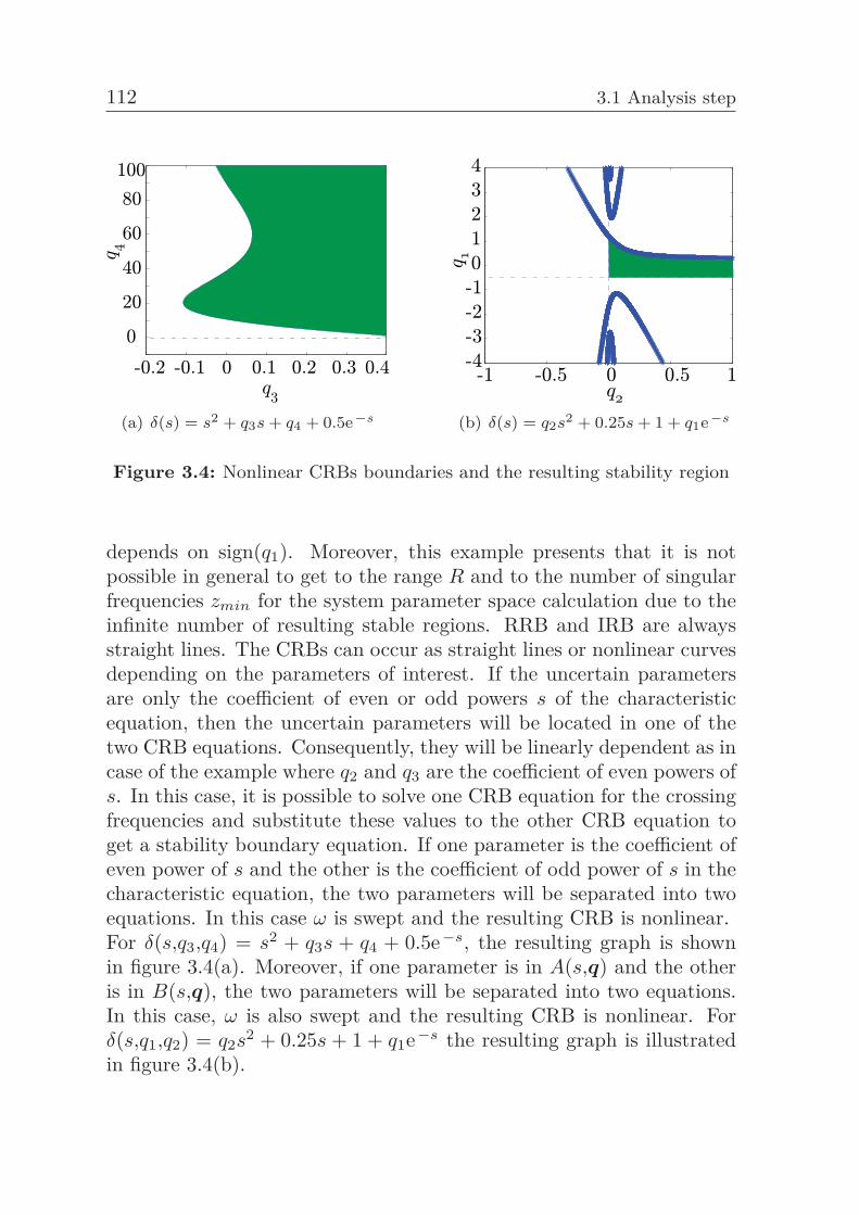
112 3.1 Analysis step
(a) δ(s) = s2 + q3s + q4 + 0.5e−s (b) δ(s) = q2s2 + 0.25s + 1 + q1e−s
Figure 3.4: Nonlinear CRBs boundaries and the resulting stability region
depends on sign(q1). Moreover, this example presents that it is notpossible in general to get to the range R and to the number of singularfrequencies zmin for the system parameter space calculation due to theinfinite number of resulting stable regions. RRB and IRB are alwaysstraight lines. The CRBs can occur as straight lines or nonlinear curvesdepending on the parameters of interest. If the uncertain parametersare only the coefficient of even or odd powers s of the characteristicequation, then the uncertain parameters will be located in one of thetwo CRB equations. Consequently, they will be linearly dependent as incase of the example where q2 and q3 are the coefficient of even powers ofs. In this case, it is possible to solve one CRB equation for the crossingfrequencies and substitute these values to the other CRB equation toget a stability boundary equation. If one parameter is the coefficient ofeven power of s and the other is the coefficient of odd power of s in thecharacteristic equation, the two parameters will be separated into twoequations. In this case ω is swept and the resulting CRB is nonlinear.For δ(s,q3,q4) = s2 + q3s + q4 + 0.5e−s, the resulting graph is shownin figure 3.4(a). Moreover, if one parameter is in A(s,q) and the otheris in B(s,q), the two parameters will be separated into two equations.In this case, ω is also swept and the resulting CRB is nonlinear. Forδ(s,q1,q2) = q2s2 + 0.25s + 1 + q1e−s the resulting graph is illustratedin figure 3.4(b).
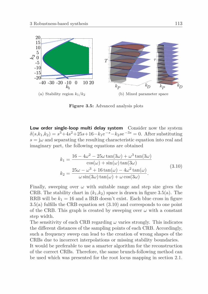
3 Robustness-based synthesis 113
(a) Stability region k1/k2 (b) Mixed parameter space
Figure 3.5: Advanced analysis plots
Low order single-loop multi delay system Consider now the systemδ(s,k1,k2) = s3+4s2+25s+16−k1e−s−k2se−3s = 0. After substitutings = jω and separating the resulting characteristic equation into real andimaginary part, the following equations are obtained
k1 =16− 4ω2 − 25ω tan(3ω) + ω3 tan(3ω)
cos(ω) + sin(ω) tan(3ω)
k2 =25ω − ω3 + 16 tan(ω)− 4ω2 tan(ω)
ω sin(3ω) tan(ω) + ω cos(3ω).
(3.10)
Finally, sweeping over ω with suitable range and step size gives theCRB. The stability chart in (k1,k2) space is drawn in figure 3.5(a). TheRRB will be k1 = 16 and a IRB doesn’t exist. Each blue cross in figure3.5(a) fulfills the CRB equation set (3.10) and corresponds to one pointof the CRB. This graph is created by sweeping over ω with a constantstep width.The sensitivity of each CRB regarding ω varies strongly. This indicatesthe different distances of the sampling points of each CRB. Accordingly,such a frequency sweep can lead to the creation of wrong shapes of theCRBs due to incorrect interpolations or missing stability boundaries.It would be preferable to use a smarter algorithm for the reconstructionof the correct CRBs. Therefore, the same brunch-following method canbe used which was presented for the root locus mapping in section 2.1.
114 3.1 Analysis step
The only change which occurs is that the search algorithm has the taskof finding the points which fulfill both CRB equations best instead ofchecking the phase condition.
3.1.3 Advanced system classes
The previously introduced ideas for creating the system parameter re-gion plots can also be adapted to the case of more complex systemclasses. Unfortunately, the calculation complexity increases for moreadvanced system classes as was shown in section 3.1.2. Therefore, itis recommended that the Lyapunov stability-based or the probabilistic-based calculation methods be used, presented in section 2.6 and 2.7.These methods do not change regarding the creating of the system pa-rameter region plots, see e.g. example 2.12. Consequently, these meth-ods are much more efficient in comparison to the analysis step of thePSA.From an usability point of view, it makes also sense to merge the syn-thesis and analysis step by calculating a parameter space which consistsof the free adjustable controller parameters as well as the uncertain sys-tem parameters, see e.g. again example 2.12. and figure 3.5(b).In figure 3.5(b) the stabilizing controller as well as system parameterspace is presented for a first order time delay system controlled by a PIDcontroller under consideration of uncertainties in the time constant Tand the time delay τ by assuming a fixed value of k∗
P . In this example,the red area represents the robust stabilizing parameter space.Next, this high dimensional parameter region has to be mapped intoa parameter space which purely consists of the controller parameters.Accordingly, several stability regions result for the different system pa-rameter combinations.Finally, the intersection area of the resulting stability regions leads tothe robust stabilizing parameter space. Such an idea for robust con-troller design by using multi-model approaches was already proposedin [4, 334]. However, tools for such complex computations were lack-ing at this time and today, the approaches need a lot of calculationtime. Therefore, some analytical methods to solve this problem moreelegantly for special classes of uncertainties are presented next.
3 Robustness-based synthesis 115
3.2 Test set-based robust controller synthesisAs extension of the classical work of [4,34,44], this section focuses on thesimplification of the PSA-based robust controller design by introducinga one-step approach which is based on the test set calculation. The ideais to calculate the controller parameter stability region for a family ofpolynomials δ(s, k∗,Q) based on a worst case set of system parametersQT ⊂ Q which build the worst case test set TS . This reduces the com-plexity of the whole method to a finite worst case set calculation. Theresult of δ(s, k∗,QT ) guaranties the stability of δ(s, k∗,Q). Therefore,the analysis step is no longer needed. The following sections focus onPID for an easier explanation of the algebraic calculation rules. Theexpansion to other controller types is easily possible.
3.2.1 Interval polynomials
An interval polynomial has the form δ(s, k∗, a) = a0 + a1s + · · ·+ ansn
with a = [a0 . . . an] ∈ A and ai ∈ [a−i ,a+
i ], a−i > 0. Therefore, it results
Q = A = [a−0 ,a+
0 ] × [a−1 ,a+
1 ] × [a−2 ,a+
2 ] × · · · × [a−n ,a+
n ]. The operatingdomain of uncertain parameters Q is similar to the set of polynomialcoefficients A which build a (n + 1)-dimensional hyper-rectangle.
Test set theory control1 The Kharitonov theorem states that an in-terval polynomial is stable if the four Kharitonov polynomials
δ−−(s, k∗, a) = a−0 + a−
1 s + a+2 s2 + a+
3 s3 + a−4 s4 + . . .
δ−+(s, k∗, a) = a−0 + a+
1 s + a+2 s2 + a−
3 s3 + a−4 s4 + . . .
δ++(s, k∗, a) = a+0 + a+
1 s + a−2 s2 + a−
3 s3 + a+4 s4 + . . .
δ+−(s, k∗, a) = a+0 + a−
1 s + a−2 s2 + a+
3 s3 + a+4 s4 + . . .
(3.11)
are stable [4]. Independent of the polynomial order n and the numberof uncertain parameters h, only four worst case conditions represent theworst case test set and have to be checked for stability to deduct the
1A first implementation and discussion of the proposed ideas have been presentedin [S28, S38]. The following section is based on this.
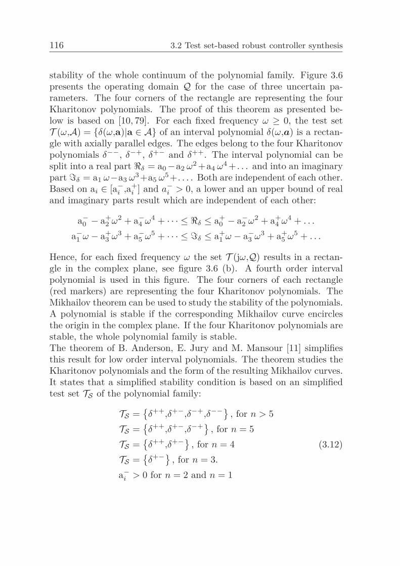
116 3.2 Test set-based robust controller synthesis
stability of the whole continuum of the polynomial family. Figure 3.6presents the operating domain Q for the case of three uncertain pa-rameters. The four corners of the rectangle are representing the fourKharitonov polynomials. The proof of this theorem as presented be-low is based on [10, 79]. For each fixed frequency ω ≥ 0, the test setT (ω,A) = {δ(ω,a)|a ∈ A} of an interval polynomial δ(ω,a) is a rectan-gle with axially parallel edges. The edges belong to the four Kharitonovpolynomials δ−−, δ−+, δ+− and δ++. The interval polynomial can besplit into a real part �δ = a0−a2 ω2 +a4 ω4 + . . . and into an imaginarypart �δ = a1 ω−a3 ω3+a5 ω5+. . . . Both are independent of each other.Based on ai ∈ [a−
i ,a+i ] and a−
i > 0, a lower and an upper bound of realand imaginary parts result which are independent of each other:
a−0 − a+
2 ω2 + a−4 ω4 + · · · ≤ �δ ≤ a+
0 − a−2 ω2 + a+
4 ω4 + . . .
a−1 ω − a+
3 ω3 + a−5 ω5 + · · · ≤ �δ ≤ a+
1 ω − a−3 ω3 + a+
5 ω5 + . . .
Hence, for each fixed frequency ω the set T (jω,Q) results in a rectan-gle in the complex plane, see figure 3.6 (b). A fourth order intervalpolynomial is used in this figure. The four corners of each rectangle(red markers) are representing the four Kharitonov polynomials. TheMikhailov theorem can be used to study the stability of the polynomials.A polynomial is stable if the corresponding Mikhailov curve encirclesthe origin in the complex plane. If the four Kharitonov polynomials arestable, the whole polynomial family is stable.The theorem of B. Anderson, E. Jury and M. Mansour [11] simplifiesthis result for low order interval polynomials. The theorem studies theKharitonov polynomials and the form of the resulting Mikhailov curves.It states that a simplified stability condition is based on an simplifiedtest set TS of the polynomial family:
TS ={
δ++,δ+−,δ−+,δ−−} , for n > 5TS =
{δ++,δ+−,δ−+} , for n = 5
TS ={
δ++,δ+−} , for n = 4TS =
{δ+−} , for n = 3.
a−i > 0 for n = 2 and n = 1
(3.12)
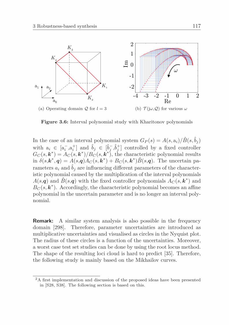
3 Robustness-based synthesis 117
(a) Operating domain Q for l = 3 (b) T (jω,Q) for various ω
Figure 3.6: Interval polynomial study with Kharitonov polynomials
In the case of an interval polynomial system GP (s) = A(s, ai)/B(s, bj)with ai ∈ [a−
i ,a+i ] and bj ∈ [b−
j ,b+j ] controlled by a fixed controller
GC(s, k∗) = AC(s, k∗)/BC(s, k∗), the characteristic polynomial resultsin δ(s,k∗, q) = A(s,q)AC(s, k∗) + BC(s, k∗)B(s,q). The uncertain pa-rameters ai and bj are influencing different parameters of the character-istic polynomial caused by the multiplication of the interval polynomialsA(s,q) and B(s,q) with the fixed controller polynomials AC(s, k∗) andBC(s, k∗). Accordingly, the characteristic polynomial becomes an affinepolynomial in the uncertain parameter and is no longer an interval poly-nomial.
Remark: A similar system analysis is also possible in the frequencydomain [298]. Therefore, parameter uncertainties are introduced asmultiplicative uncertainties and visualised as circles in the Nyquist plot.The radius of these circles is a function of the uncertainties. Moreover,a worst case test set studies can be done by using the root locus method.The shape of the resulting loci cloud is hard to predict [35]. Therefore,the following study is mainly based on the Mikhailov curves.
2A first implementation and discussion of the proposed ideas have been presentedin [S28, S38]. The following section is based on this.
118 3.2 Test set-based robust controller synthesis
PID controlled systems with constant A(s)2 Such a transfer func-tion is an often used system model in the industrial praxis. For the caseof a PID controlled system with fixed system gains (constant A(s)), theresults of the Kharitonov theorem and the PSA can be directly appliedfor the calculation of all stabilizing controller parameters KQ which sta-bilize the whole operating domain. In this case, the characteristic poly-nomial is: δ(s, k∗, q) = A(s)
(kDs2 + kP s + kI
)+ s B(s,q). Due to the
fact that the controller gains are constant the characteristic equation isan interval polynomial because each uncertain parameter bj influencesonly one coefficient of the polynomial. Therefore, the Kharitonov theo-rem can be used if a−
i > 0. The set of stabilizing controller parametersKQ can be calculated through the use of the stability region calcula-tion for the four Kharitonov polynomials δ++, δ+−, δ−+ and δ−−. Theintersection area of the stability sets represents the robust stabilizingcontroller parameter space
KQ =⋂
i
Kδi , i ∈ {+ + , +−,−+,−−}. (3.13)
Example 3.1. Consider a mass spring damper system controlled by aPID controller. The characteristic polynomial is: δ(s, k∗, q) = m s3 +(kD + c) s2 + (kP + k) s + kI with an uncertain mass m ∈ [2,20] andspring constant c ∈ [0.1,1]. Accordingly, a third order interval polyno-mial results. The stability can be checked using the Kharitonov poly-nomial δ+−(s, k∗, q) = m+s3 +
(kD + c−) s2 + (kP + k) s + kI . With
focusing on the CRB figure 3.7 presents the resulting stability region fordifferent values m and c of the operating domain Q (blue lines) and forδ+− (red line). The red stability boundary is the worst case boundarywhich forms the stable region (green area). The controller parametersinside this region stabilizes the whole polynomial family δ(s, k∗,Q).
General order interval systems with first order controller3 It is pos-sible to calculate the robust stabilizing controller parameter space basedon a finite test set for a general order interval system GP = A(s,q)/B,q(s)
3A first implementation and discussion of the proposed ideas have been presentedin [S28, S38]. The following section is based on this.
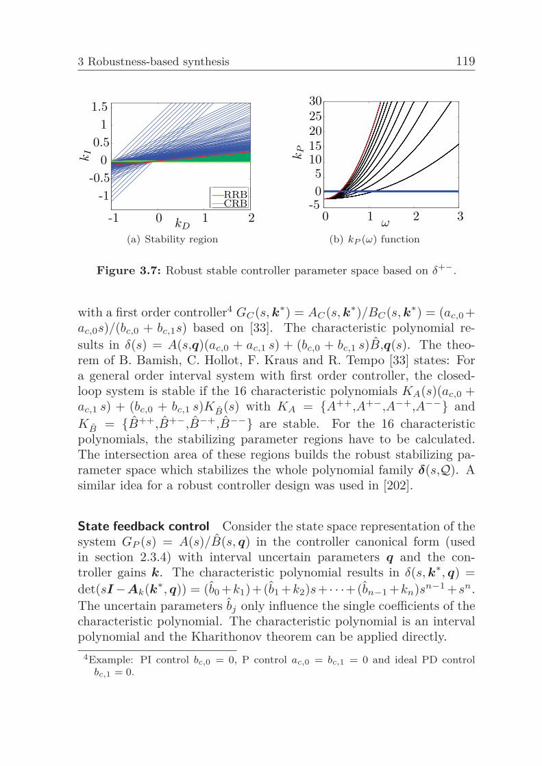
3 Robustness-based synthesis 119
-1 0 1 2
-1-0.5
00.5
11.5
kI
kD
RRBCRB
(a) Stability region
0 1 2
05
10
3ω
kP 15
202530
-5
(b) kP (ω) function
Figure 3.7: Robust stable controller parameter space based on δ+−.
with a first order controller4 GC(s, k∗) = AC(s, k∗)/BC(s, k∗) = (ac,0 +ac,0s)/(bc,0 + bc,1s) based on [33]. The characteristic polynomial re-sults in δ(s) = A(s,q)(ac,0 + ac,1 s) + (bc,0 + bc,1 s)B,q(s). The theo-rem of B. Bamish, C. Hollot, F. Kraus and R. Tempo [33] states: Fora general order interval system with first order controller, the closed-loop system is stable if the 16 characteristic polynomials KA(s)(ac,0 +ac,1 s) + (bc,0 + bc,1 s)KB(s) with KA = {A++,A+−,A−+,A−−} andKB = {B++,B+−,B−+,B−−} are stable. For the 16 characteristicpolynomials, the stabilizing parameter regions have to be calculated.The intersection area of these regions builds the robust stabilizing pa-rameter space which stabilizes the whole polynomial family δ(s,Q). Asimilar idea for a robust controller design was used in [202].
State feedback control Consider the state space representation of thesystem GP (s) = A(s)/B(s, q) in the controller canonical form (usedin section 2.3.4) with interval uncertain parameters q and the con-troller gains k. The characteristic polynomial results in δ(s, k∗, q) =det(sI−Ak(k∗, q)) = (b0 +k1)+(b1 +k2)s+ · · ·+(bn−1 +kn)sn−1 +sn.The uncertain parameters bj only influence the single coefficients of thecharacteristic polynomial. The characteristic polynomial is an intervalpolynomial and the Kharithonov theorem can be applied directly.
4Example: PI control bc,0 = 0, P control ac,0 = bc,1 = 0 and ideal PD controlbc,1 = 0.
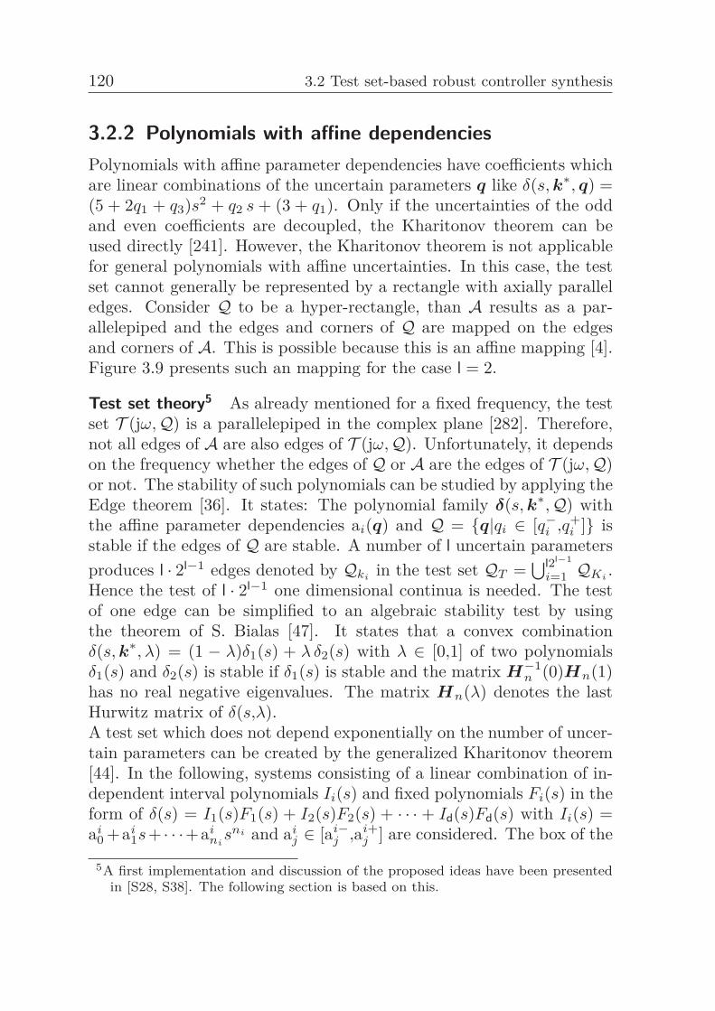
120 3.2 Test set-based robust controller synthesis
3.2.2 Polynomials with affine dependenciesPolynomials with affine parameter dependencies have coefficients whichare linear combinations of the uncertain parameters q like δ(s, k∗, q) =(5 + 2q1 + q3)s2 + q2 s + (3 + q1). Only if the uncertainties of the oddand even coefficients are decoupled, the Kharitonov theorem can beused directly [241]. However, the Kharitonov theorem is not applicablefor general polynomials with affine uncertainties. In this case, the testset cannot generally be represented by a rectangle with axially paralleledges. Consider Q to be a hyper-rectangle, than A results as a par-allelepiped and the edges and corners of Q are mapped on the edgesand corners of A. This is possible because this is an affine mapping [4].Figure 3.9 presents such an mapping for the case l = 2.
Test set theory5 As already mentioned for a fixed frequency, the testset T (jω,Q) is a parallelepiped in the complex plane [282]. Therefore,not all edges of A are also edges of T (jω,Q). Unfortunately, it dependson the frequency whether the edges of Q or A are the edges of T (jω,Q)or not. The stability of such polynomials can be studied by applying theEdge theorem [36]. It states: The polynomial family δ(s, k∗,Q) withthe affine parameter dependencies ai(q) and Q = {q|qi ∈ [q−
i ,q+i ]} is
stable if the edges of Q are stable. A number of l uncertain parametersproduces l · 2l−1 edges denoted by Qki in the test set QT =
⋃l2l−1
i=1 QKi .Hence the test of l · 2l−1 one dimensional continua is needed. The testof one edge can be simplified to an algebraic stability test by usingthe theorem of S. Bialas [47]. It states that a convex combinationδ(s, k∗, λ) = (1 − λ)δ1(s) + λ δ2(s) with λ ∈ [0,1] of two polynomialsδ1(s) and δ2(s) is stable if δ1(s) is stable and the matrix H−1
n (0)Hn(1)has no real negative eigenvalues. The matrix Hn(λ) denotes the lastHurwitz matrix of δ(s,λ).A test set which does not depend exponentially on the number of uncer-tain parameters can be created by the generalized Kharitonov theorem[44]. In the following, systems consisting of a linear combination of in-dependent interval polynomials Ii(s) and fixed polynomials Fi(s) in theform of δ(s) = I1(s)F1(s) + I2(s)F2(s) + · · · + Id(s)Fd(s) with Ii(s) =ai
0 +ai1s+ · · ·+ai
nisni and ai
j ∈ [ai−j ,ai+
j ] are considered. The box of the
5A first implementation and discussion of the proposed ideas have been presentedin [S28, S38]. The following section is based on this.
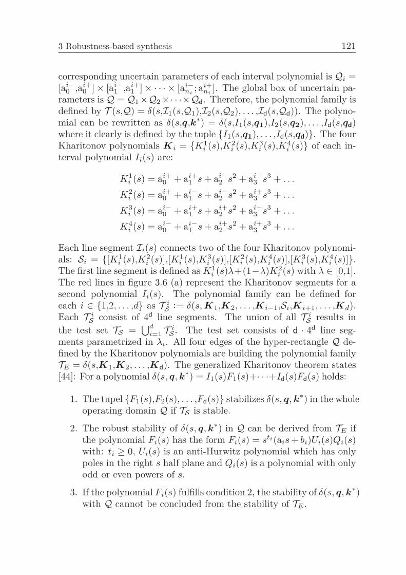
3 Robustness-based synthesis 121
corresponding uncertain parameters of each interval polynomial is Qi =[ai−
0 ,ai+0 ]× [ai−
1 ,ai+1 ]× · · · × [ai−
ni; ai+
ni]. The global box of uncertain pa-
rameters is Q = Q1×Q2×· · ·×Qd. Therefore, the polynomial family isdefined by T (s,Q) = δ(s,I1(s,Q1),I2(s,Q2), . . . ,Id(s,Qd)). The polyno-mial can be rewritten as δ(s,q,k∗) = δ(s,I1(s,q1),I2(s,q2), . . . ,Id(s,qd)where it clearly is defined by the tuple {I1(s,q1), . . . ,Id(s,qd)}. The fourKharitonov polynomials Ki = {K1
i (s),K2i (s),K3
i (s),K4i (s)} of each in-
terval polynomial Ii(s) are:
K1i (s) = ai+
0 + ai+1 s + ai−
2 s2 + ai−3 s3 + . . .
K2i (s) = ai+
0 + ai−1 s + ai−
2 s2 + ai+3 s3 + . . .
K3i (s) = ai−
0 + ai+1 s + ai+
2 s2 + ai−3 s3 + . . .
K4i (s) = ai−
0 + ai−1 s + ai+
2 s2 + ai+3 s3 + . . .
Each line segment Ii(s) connects two of the four Kharitonov polynomi-als: Si = {[K1
i (s),K2i (s)],[K1
i (s),K3i (s)],[K2
i (s),K4i (s)],[K3
i (s),K4i (s)]}.
The first line segment is defined as K1i (s)λ+(1−λ)K2
i (s) with λ ∈ [0,1].The red lines in figure 3.6 (a) represent the Kharitonov segments for asecond polynomial Ii(s). The polynomial family can be defined foreach i ∈ {1,2, . . . ,d} as T i
S := δ(s, K1,K2, . . . ,Ki−1,Si,Ki+1, . . . ,Kd).Each T i
S consist of 4d line segments. The union of all T iS results in
the test set TS =⋃d
i=1 T iS . The test set consists of d · 4d line seg-
ments parametrized in λi. All four edges of the hyper-rectangle Q de-fined by the Kharitonov polynomials are building the polynomial familyTE = δ(s,K1,K2, . . . ,Kd). The generalized Kharitonov theorem states[44]: For a polynomial δ(s, q, k∗) = I1(s)F1(s)+· · ·+Id(s)Fd(s) holds:
1. The tupel {F1(s),F2(s), . . . ,Fd(s)} stabilizes δ(s, q, k∗) in the wholeoperating domain Q if TS is stable.
2. The robust stability of δ(s, q, k∗) in Q can be derived from TE ifthe polynomial Fi(s) has the form Fi(s) = sti(ais + bi)Ui(s)Qi(s)with: ti ≥ 0, Ui(s) is an anti-Hurwitz polynomial which has onlypoles in the right s half plane and Qi(s) is a polynomial with onlyodd or even powers of s.
3. If the polynomial Fi(s) fulfills condition 2, the stability of δ(s, q, k∗)with Q cannot be concluded from the stability of TE .
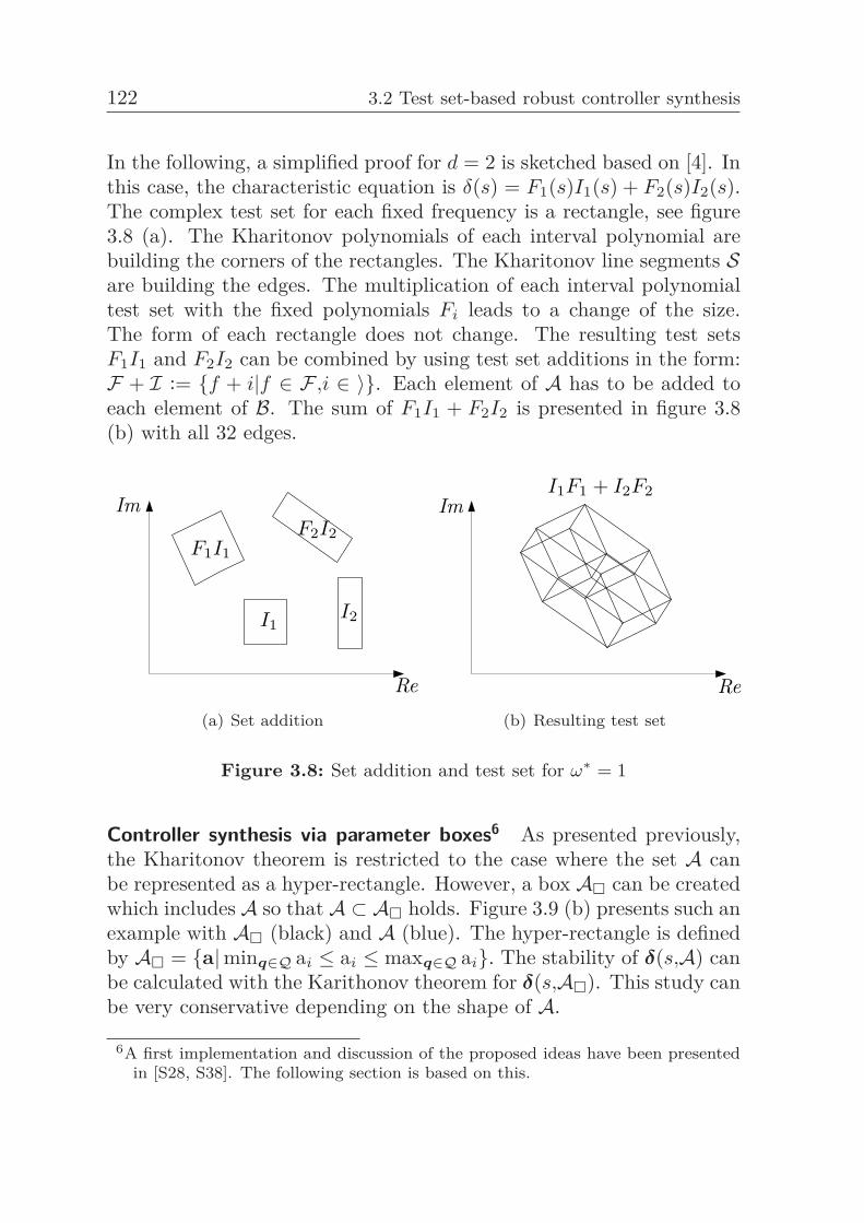
122 3.2 Test set-based robust controller synthesis
In the following, a simplified proof for d = 2 is sketched based on [4]. Inthis case, the characteristic equation is δ(s) = F1(s)I1(s) + F2(s)I2(s).The complex test set for each fixed frequency is a rectangle, see figure3.8 (a). The Kharitonov polynomials of each interval polynomial arebuilding the corners of the rectangles. The Kharitonov line segments Sare building the edges. The multiplication of each interval polynomialtest set with the fixed polynomials Fi leads to a change of the size.The form of each rectangle does not change. The resulting test setsF1I1 and F2I2 can be combined by using test set additions in the form:F + I := {f + i|f ∈ F ,i ∈ 〉}. Each element of A has to be added toeach element of B. The sum of F1I1 + F2I2 is presented in figure 3.8(b) with all 32 edges.
Im
F1I1F2I2
I1I2
Re(a) Set addition
Im
Re
I1F1 + I2F2
(b) Resulting test set
Figure 3.8: Set addition and test set for ω∗ = 1
Controller synthesis via parameter boxes6 As presented previously,the Kharitonov theorem is restricted to the case where the set A canbe represented as a hyper-rectangle. However, a box A� can be createdwhich includes A so that A ⊂ A� holds. Figure 3.9 (b) presents such anexample with A� (black) and A (blue). The hyper-rectangle is definedby A� = {a|minq∈Q ai ≤ ai ≤ maxq∈Q ai}. The stability of δ(s,A) canbe calculated with the Karithonov theorem for δ(s,A�). This study canbe very conservative depending on the shape of A.
6A first implementation and discussion of the proposed ideas have been presentedin [S28, S38]. The following section is based on this.
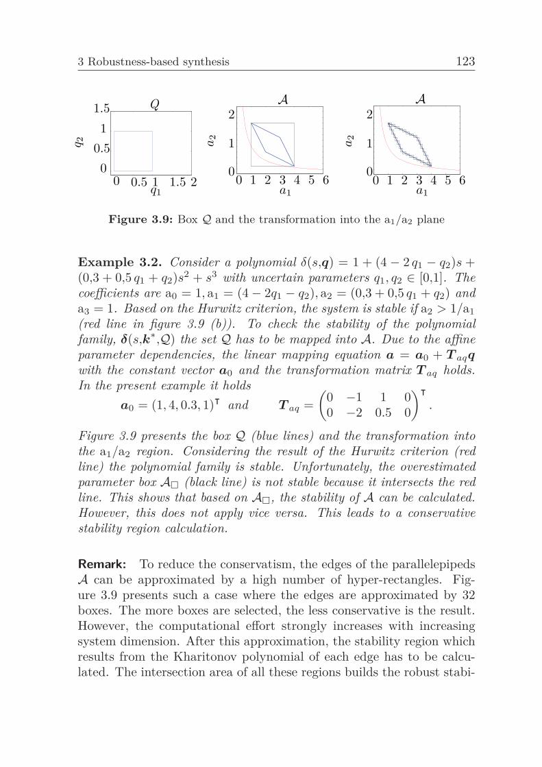
3 Robustness-based synthesis 123
Q
0.51
00 0.5 1 1.5 2
q1
q 2
1.5A
1
2
00 1 2 3 4 5 6a1
a2
A
1
2
00 1 2 3 4 5 6
a1
a2
Figure 3.9: Box Q and the transformation into the a1/a2 plane
Example 3.2. Consider a polynomial δ(s,q) = 1 + (4 − 2 q1 − q2)s +(0,3 + 0,5 q1 + q2)s2 + s3 with uncertain parameters q1, q2 ∈ [0,1]. Thecoefficients are a0 = 1, a1 = (4− 2q1 − q2), a2 = (0,3 + 0,5 q1 + q2) anda3 = 1. Based on the Hurwitz criterion, the system is stable if a2 > 1/a1(red line in figure 3.9 (b)). To check the stability of the polynomialfamily, δ(s,k∗,Q) the set Q has to be mapped into A. Due to the affineparameter dependencies, the linear mapping equation a = a0 + T aqqwith the constant vector a0 and the transformation matrix T aq holds.In the present example it holds
a0 = (1, 4, 0.3, 1)ᵀ and T aq =(
0 −1 1 00 −2 0.5 0
)ᵀ.
Figure 3.9 presents the box Q (blue lines) and the transformation intothe a1/a2 region. Considering the result of the Hurwitz criterion (redline) the polynomial family is stable. Unfortunately, the overestimatedparameter box A� (black line) is not stable because it intersects the redline. This shows that based on A�, the stability of A can be calculated.However, this does not apply vice versa. This leads to a conservativestability region calculation.
Remark: To reduce the conservatism, the edges of the parallelepipedsA can be approximated by a high number of hyper-rectangles. Fig-ure 3.9 presents such a case where the edges are approximated by 32boxes. The more boxes are selected, the less conservative is the result.However, the computational effort strongly increases with increasingsystem dimension. After this approximation, the stability region whichresults from the Kharitonov polynomial of each edge has to be calcu-lated. The intersection area of all these regions builds the robust stabi-
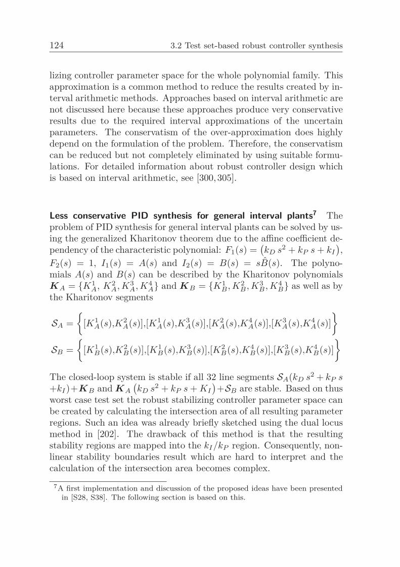
124 3.2 Test set-based robust controller synthesis
lizing controller parameter space for the whole polynomial family. Thisapproximation is a common method to reduce the results created by in-terval arithmetic methods. Approaches based on interval arithmetic arenot discussed here because these approaches produce very conservativeresults due to the required interval approximations of the uncertainparameters. The conservatism of the over-approximation does highlydepend on the formulation of the problem. Therefore, the conservatismcan be reduced but not completely eliminated by using suitable formu-lations. For detailed information about robust controller design whichis based on interval arithmetic, see [300,305].
Less conservative PID synthesis for general interval plants7 Theproblem of PID synthesis for general interval plants can be solved by us-ing the generalized Kharitonov theorem due to the affine coefficient de-pendency of the characteristic polynomial: F1(s) =
(kD s2 + kP s + kI
),
F2(s) = 1, I1(s) = A(s) and I2(s) = B(s) = sB(s). The polyno-mials A(s) and B(s) can be described by the Kharitonov polynomialsKA = {K1
A, K2A, K3
A, K4A} and KB = {K1
B , K2B , K3
B , K4B} as well as by
the Kharitonov segments
SA ={
[K1A(s),K2
A(s)],[K1A(s),K3
A(s)],[K2A(s),K4
A(s)],[K3A(s),K4
A(s)]}
SB ={
[K1B(s),K2
B(s)],[K1B(s),K3
B(s)],[K2B(s),K4
B(s)],[K3B(s),K4
B(s)]}
The closed-loop system is stable if all 32 line segments SA(kD s2 + kP s+kI)+KB and KA
(kD s2 + kP s + KI
)+SB are stable. Based on thus
worst case test set the robust stabilizing controller parameter space canbe created by calculating the intersection area of all resulting parameterregions. Such an idea was already briefly sketched using the dual locusmethod in [202]. The drawback of this method is that the resultingstability regions are mapped into the kI/kP region. Consequently, non-linear stability boundaries result which are hard to interpret and thecalculation of the intersection area becomes complex.
7A first implementation and discussion of the proposed ideas have been presentedin [S28, S38]. The following section is based on this.
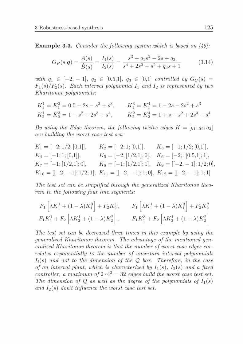
3 Robustness-based synthesis 125
Example 3.3. Consider the following system which is based on [46]:
GP (s,q) =A(s)B(s)
=I1(s)I2(s)
=s3 + q1s2 − 2s + q2
s4 + 2s3 − s2 + q3s + 1(3.14)
with q1 ∈ [−2, − 1], q2 ∈ [0.5,1], q3 ∈ [0,1] controlled by GC(s) =F1(s)/F2(s). Each interval polynomial I1 and I2 is represented by twoKharitonov polynomials:
K11 = K2
1 = 0.5− 2s− s2 + s3, K31 = K4
1 = 1− 2s− 2s2 + s3
K12 = K3
2 = 1− s2 + 2s3 + s4, K22 = K4
2 = 1 + s− s2 + 2s3 + s4
By using the Edge theorem, the following twelve edges K = [q1; q2; q3]are building the worst case test set:
K1 = [−2; 1/2; [0,1]], K2 = [−2; 1; [0,1]], K3 = [−1; 1/2; [0,1]],K4 = [−1; 1; [0,1]], K5 = [−2; [1/2,1]; 0], K6 = [−2; ; [0.5,1]; 1],K7 = [−1; [1/2,1]; 0], K8 = [−1; [1/2,1]; 1], K9 = [[−2,− 1]; 1/2; 0],K10 = [[−2,− 1]; 1/2; 1], K11 = [[−2,− 1]; 1; 0], K12 = [[−2,− 1]; 1; 1]
The test set can be simplified through the generalized Kharitonov theo-rem to the following four line segments:
F1
[λK1
1 + (1− λ)K31
]+ F2K1
2 , F1
[λK1
1 + (1− λ)K31
]+ F2K2
2
F1K11 + F2
[λK1
2 + (1− λ)K22
], F1K3
1 + F2
[λK1
2 + (1− λ)K22
]The test set can be decreased three times in this example by using thegeneralized Kharitonov theorem. The advantage of the mentioned gen-eralized Kharitonov theorem is that the number of worst case edges cor-relates exponentially to the number of uncertain interval polynomialsIi(s) and not to the dimension of the Q box. Therefore, in the caseof an interval plant, which is characterized by I1(s), I2(s) and a fixedcontroller, a maximum of 2 · 42 = 32 edges build the worst case test set.The dimension of Q as well as the degree of the polynomials of I1(s)and I2(s) don’t influence the worst case test set.
126 3.2 Test set-based robust controller synthesis
Controller synthesis via boundary movement analysis8 For the syn-thesis of polynomials with affine uncertainties it was demonstrated thatthe test set contains line segments. Let’s consider a plant GP (s,q) =A(s,q)/B(s,q) where the polynomials can be described by the followinglinear combinations A(s,q) = A0(s)+λAΔ(s); B(s,q) = B0(s)+λBΔ(s)and λ ∈ [0,1]. The real and imaginary part of these polynomials are�A = �A0 + λ�AΔ , �A = �A0 + λ�AΔ , �B = �B0
+ λ�BΔand
�B = �B0+ λ�BΔ
. The polynomials A0(s), AΔ(s), B0(s) and BΔ(s)are constant. Therefore, a mapping approach for linear combinationswill be presented based on the analysis of the stability boundary move-ment. As mentioned before the RRB does not depend on the systemparameters. Accordingly, the stability boundary remains constant in-dependently of the system uncertainties.The IRB is defined by kD = −bn/am for n = m + 2. After substitutingthe uncertain polynomials, an IRB band results parallel to the kI axis.The width of the band is given by λ ∈ [0; 1]. Therefore, it results:
kD = − b0n + λbΔ
n
a0m + λaΔ
m
⇒ ∂kD
∂λ= −bΔ
n a0m − b0
naΔm(
a0m + λaΔ
m
)2
In the case bΔn a0
m − b0naΔ
m �= 0, the border of the IRB band is definedby kD(λ = 0) and kD(λ = 1). For bΔ
n a0m − b0
naΔm = 0, kD(λ = 0) and
kD(λ = 1) are the same. Consequently, the IRB band degenerates to aline. Due to the uncertainty, a whole family of CRBs results which issimilarly to the IRB case. The calculation for the enveloping CRB isbased on the CRB kinetic study in section 2.3.1. By varying λ ∈ [0,1],the CRB rotates along the i.c.r. Ip. The i.c.r trajectory is calculatedthrough the differentiation of the CRB equation:
∂kI
∂λ= 2ω
∂ω
∂λkIp
D +∂k0
I
∂λ= 0 with kIp
D = − 12ω
∂k0I
∂λ
∂λ
∂ω
The derivative of the singular frequency with respect to λ can be cal-culated numerically. This numerical procedure corresponds to gridingthe CRBs next to the i.c.r. . Due to the continuous movement of the
8A first implementation and discussion of the proposed ideas have been presentedin [S28, S38]. The following section is based on this.
3 Robustness-based synthesis 127
CRB no big error should occur. The derivative of k0I is:
∂k0I
∂λ= ∂
∂λ
(kP ω�A − �B
�A
)= kP
[∂ω
∂λ
�A
�A+ ω
(∂�A
∂λ�A − ∂�A
∂λ�A
)/�2
A
]
−∂�B
∂λ�A − ∂�A
∂λ�B
�2A
with ∂�A
∂λ=
∂(�A0 + λ�AΔ
)∂λ
= ∂�A0
∂ω
∂ω
λ
+ �AΔ + λ∂�AΔ
∂ω
∂ω
∂λ=
∂(�A0 + λ�AΔ
)∂ω
∂ω
∂λ+ �AΔ = ∂�A
∂ω
∂ω
∂λ+ �AΔ
The other differentiations can be realized similarly:
∂k0I
∂λ=kP
⎡⎢⎢⎢⎣∂ω
∂λ
�A
�A+ ω
(∂�A
∂ω
∂ω
∂λ+ �AΔ
)�A −
(∂�A
∂ω
∂ω
∂λ+ �AΔ
)�A
�2A
⎤⎥⎥⎥⎦−
((∂�B
∂ω
∂ω
∂λ+ �BΔ
)�A −
(∂�A
∂ω
dω
dλ+ �AΔ
)�B
)/�2
A
Substituting ∂k0I /∂λ into the CRB equation, the i.c.r for kI results:
kIpI = ω2kIp
D + k0I = −1
2ω
∂k0I
∂λ
∂λ
∂ω+ k0
I
Similar to section 2.3.1, the slope of the i.r.c. tangent can be calculatedbased on dkIp
I /dkIpD:
∂kIpI
∂λ= −1
2∂k0
I
∂λ− 1
2ω
∂2k0I
∂λ2∂λ
∂ω+ 1
2ω
∂k0I
∂λ
∂2ω
∂λ2
(∂λ
∂ω
)2
+ ∂k0I
∂λ
∂kIpD
∂λ
∂kIpD
∂λ= 1
2ω2∂k0
I
∂λ− 1
2ω
∂2k0I
∂λ2∂λ
∂ω+ 1
2ω
∂k0I
∂λ
∂2ω
∂λ2
(∂λ
∂ω
)2
The slope in the tangent results in ∂k0I /∂kIp
D = ω2. All CRBs aretouching the resulting i.c.r. trajectory tangentially. The whole CRBfamily can be replaced by using the resulting i.c.r. trajectory togetherwith the CRBs corresponding to λ = 0 and λ = 1. In figure 3.10, the tworesulting cases are presented. In the first case, the CRBs corresponding
128 3.2 Test set-based robust controller synthesis
to λ = 0 and λ = 1 are bounding the stability region and the CRB i.c.r.trajectory is located in the unstable region. In the second case, the CRBi.c.r. trajectory and the CRBs for λ = 0 and λ = 1 bound the stabilityregion together. For a practical implementation it is desirable to checkif the first case is present before the CRB i.c.r. trajectory calculation isstarted. This can be done by using the Vertex theorem [44]. Considerthe two polynomials δ1(s) and δ2(s). The stability of the line segment[δ1(s),δ2(s)] can be deduced through the stability of the endpoints δ1(s)and δ2(s). This holds if the difference of the polynomials δ1(s) and δ2(s)can be expressed as δ0(s) = δ2(s)−δ1(s) = st(as+b)U(s)Q(s) with t ∈ N
an anti-Hurwitz polynomial U(s) and a polynomial Q(s) with only evenor odd power of s. For a system AΔ(s) = 0 the difference polynomialis δ0(s) = BΔ. If this polynomial satisfies the Vertex theorem it issufficient to consider only the ends of the polynomial segments. In suchcase, the CRB i.c.r. trajectory doesn’t have to be calculated. TheVertex theorem is only necessary and not sufficient. Accordingly, theVertex theorem fails in some cases but the CRB i.c.r. trajectory doesn’tbound the stability area.
Example 3.4. Again consider the spring mass damper system whichis controlled by a PID controller. Assume the uncertainties which aredescribed in figure 3.10 (a). In the following, k∗
P = 0.5 and k∗ = 2 aregiven. The polynomials are A0 = 1, AΔ = 0, B0 = s(s2 + 2s + 2) andBΔ = s(19s2+3s) with A = 1 and B = s
[(1 + 19λ) s2 + (2 + 3λ) s + 2
].
Therefore, it results
∂k0I
∂λ= −∂�B
∂ω
∂ω
∂λ−�BΔ with ∂�B
∂ω= −2(2 + 3λ)ω and
�BΔ = −3ω2. This leads to
kIpD = − 1
2ω
[2
∂ω
∂λ(2 + 3λ)ω + 3ω2
]∂λ
∂ω= −(2 + 3λ)− 3
2ω
∂λ
∂ωwith
ω =√
kP + 21 + 19λ
and ∂ω
∂λ= −19
2√
kP + 2(1 + 19λ)− 32 ⇒ kIp
D = −2 +319
.
It can be seen that kIpD is not a function of λ. Therefore, the CRB
i.c.r. trajectory degenerates to a single point. To plot the stabilizingcontroller parameter space in the kD/kI plane, the CRB with λ = 0 for
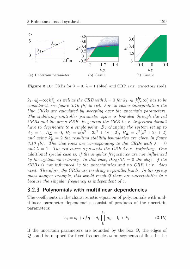
3 Robustness-based synthesis 129
c5
31 20 m
λ1
λ2
(a) Uncertain parameter
0
-2 -1.7 -1.4
0.20.40.60.8
-0.2
kI
kD
(b) Case 1
-0.4 0
3.23.4
3
kI
kD
0.4
3.6
(c) Case 2
Figure 3.10: CRBs for λ = 0, λ = 1 (blue) and CRB i.c.r. trajectory (red)
kD ∈]−∞; kIpD] as well as the CRB with λ = 0 for kD ∈ [kIp
D,∞) has to beconsidered, see figure 3.10 (b) in red. For an easier interpretation theblue CRBs are calculated by sweeping over the uncertain parameters.The stabilizing controller parameter space is bounded through the redCRBs and the green RRB. In general the CRB i.c.r. trajectory doesn’thave to degenerate to a single point. By changing the system set up toA0 = 1, AΔ = 0, B0 = s(s3 + 3s2 + 4s + 2), BΔ = s2(s2 + 2s + 2)and using k∗
P = 2 the resulting stability boundaries are given in figure3.10 (b). The blue lines are corresponding to the CRBs with λ = 0and λ = 1. The red curve represents the CRB i.c.r. trajectory. Oneadditional special case is, if the singular frequencies are not influencedby the system uncertainty. In this case, ∂ωS/∂λ = 0 the slope of theCRBs is not influenced by the uncertainties and no CRB i.c.r. doesexist. Therefore, the CRBs are resulting in parallel bands. In the springmass damper example, this would result if there are uncertainties in cbecause the singular frequency is independent of c.
3.2.3 Polynomials with multilinear dependenciesThe coefficients in the characteristic equation of polynomials with mul-tilinear parameter dependencies consist of products of the uncertainparameters:
ai = bi + cᵀi q + di
ki∏li
qli , li < ki (3.15)
If the uncertain parameters are bounded by the box Q, the edges ofQ could be mapped for fixed frequencies ω on segments of lines in the
130 3.2 Test set-based robust controller synthesis
complex domain. However, the edges of Q are not representing thewhole boundary of the resulting test set T (jω, q) in the complex domain.In the case of multilinear uncertainty dependencies, inner points of Qcan be located on the boundary of T (jω, q). Therefore, the identificationof a simple test set QT ⊂ Q like in the previous sections is not possiblein general [4, 282]. This problem is pointed out by using the followingexample, based on [3]. Consider a polynomial
δ(s,q) = a0(q) + a1(q)s + a2(q)s2 + s3 with
a0(q) = l(l− 1) + r2 + 2(l + 1)l∑
i=1qi + 2
l−1∑i=1
l∑j=i+1
qiqj
a1(q) = l +l∑
i=1qi and a2(q) = a1(q).
Based on the Hurwitz stability test, the system is stable if ai > 0,∀i ∈{1,2, . . . ,l} and a2 a1−a0 =
∑li=1(qi−1)2−r2 > 0. All positive qi fulfill
the first condition. The second condition represents a l dimensionalhyper-sphere with the origin q0 = (1 1 1 . . . 1)ᵀ and the radius r. Allparameters from the inside of the system are leading to an unstablesystem even though all corners and edges of Q are stable. This showsthat unstable islands can exist in the case of multilinear dependencies.For r → 0 the sphere degenerates to an single point. By using griding-based stability region calculation methods like in section 2.7, it is nearlyimpossible to prevent missing such isolated points.
Test set theory9 The Desoer theorem [349] states: The test set is in-cluded in the convex envelope of the corners of the operating domainQ : δ(jω,Q) ⊂ {conv, δ(jω,q), qi ∈ [q−
i ,q+i ], i = 1, . . . ,l}. If the con-
vex envelope represents a stable behavior, the system is robust stable.If the convex envelope does not represent a stable behavior, no state-ment about the stability of the polynomial family is possible becausethis theorem uses an over-approximation of the test set. This prob-lem can be solved by the division of Q which is a family of subsetsQ = Q1 ∪Q2 ∪ · · · ∪Qn, similar to section 3.2.2. From a practical point
9A first implementation and discussion of the proposed ideas have been presentedin [S28, S38]. The following section is based on this.
3 Robustness-based synthesis 131
of view, the implementation of a general applicable decision strategy forthis set splitting is very complex [282].An analytical condition for finding the exact inner set of uncertain pa-rameters which are located on the boundary of the test set is developedin [4, 282]. Consider the nominal system δ(ω, q0) with two uncertainparameters which are located on the boundary of the test set for a fixedfrequency ω. For every infinitesimal variation of the two uncertain pa-rameters q = q0 + [dq1 dq2]ᵀ, the polynomial changes to:
δ(jω, q) = δ(jω, q0) +∂δ(jω, q)
∂q1
∣∣∣∣q0
dq1 +∂δ(jω, q)
∂q2
∣∣∣∣q0
dq2
Is the polynomial still located on the boundary of the test set it can onlymove tangentially to the envelope. Therefore, both partial derivativeshave to be collinear. Based on this the condition for the mapping ofan inner point to the boundary of the test set can be stated as follows:∂δ(jω, q)/∂q1|q0 = λ ∂δ(jω, q)/∂q2|q0 with λ ∈ R. After splitting thepolynomial into real/imaginary part and using the cross product thecondition can be reformulated:
⎛⎜⎝ ∂�δ(jω,q)∂q1
∂�δ(jω,q)∂q1
⎞⎟⎠×
⎛⎜⎝ ∂�δ(jω,q)∂q2
∂�δ(jω,q)∂q2
⎞⎟⎠ = det
J︷ ︸︸ ︷⎛⎜⎝∂�δ(jω,q)∂q1
∂�δ(jω,q)∂q2
�δ(jω,q)∂q1
∂�δ(jω,q)∂q2
⎞⎟⎠ = 0
Reformulating the polynomial in the form δ(jω,q) = δ0(jω)+q1δ1(jω)+q2δ2(jω)+q1q2δ3(jω), the partial derivatives are ∂δ(jω,q)/∂q1 = δ1(jω)+q2δ3(jω) and ∂δ(jω,q)/∂q2 = δ2(jω) + q1δ3(jω). This results in:
det(�1 + �3q2 �2 + �3q1�1 + �3q2 �2 + �3q1
)=0
⇒ �1�2 −�2�1 + q1 (�1�3 −�3�1) + q2 (�3�2 −�2�3) =0
This equation is named Jacobi condition and represents a linear equa-tion in the Q plane for a fixed frequency. An easy calculation of thecritical points which are based on this condition is not possible for thegeneral case because the Jacobi condition is frequency dependent.However, for the case of two uncertain parameters, the boundary cross-
132 3.2 Test set-based robust controller synthesis
ing theorem for multilinear polynomial family can be applied based on[181]: A multilinear polynomial family with two uncertain parametersis robust stable if the corners of the operating domain Q are stable andthe equation set: �δ(jω,q) = 0, �δ(jω,q) = 0 and det J = 0 does nothave real solutions in Q. In the case of more uncertain parameters theJacobi matrix becomes:
J =
⎛⎜⎝∂�δ(jω,q)∂q1
∂�δ(jω,q)∂q2
. . .∂�δ(jω,q)
∂ql∂�δ(jω,q)
∂q1
∂�δ(jω,q)∂q2
. . .∂�δ(jω,q)
∂ql
⎞⎟⎠ (3.16)
Therefore, the stability condition results based on [181] to the followingcondition: The surface of the operating domain Q is stable and theequation set �δ(jω,q) = 0, �δ(jω,q) = 0 and det J = 0 don’t have realsolutions in Q. Keep in mind that the resulting Jacobi matrix is nolonger quadratic. Accordingly, the Jacobi condition has to be modifiedin order to check if the rank of the matrix is decreasing. In general,the computational effort for this approach increases rapidly with thenumber of uncertain parameters [282].
Test set for multilinear interval polynomials10 Consider a character-istic polynomial in the form δ(s) = F1(s)I11(s)I12(s)+F2(s)I21(s)I22(s)with the fixed controller polynomial Fi(s) and the independent intervalpolynomials Iij(s). The calculation of a simple test set for the men-tioned polynomial structure is possible, based on [44]. Four Kharitonovpolynomials Kij(s) and four Kharitonov segments Sij(s) have to be setup for each interval polynomial. The test set is TS = T 1
S⋃T 2
S with
T 1S = F1(s)S11(s)S12(s) + F2(s)K21(s)K22(s)T 2
S = F1(s)K11(s)K12(s) + F2(s)S21(s)S22(s)(3.17)
If all Kharitonov polynomials exist and are not equal, the test set TScontains 512 two dimensional continua. This test set is independent ofthe number of uncertain parameters.
10A first implementation and discussion of the proposed ideas have been presentedin [S28, S38]. The following section is based on this.
11A first implementation and discussion of the proposed ideas have been presentedin [S28, S38]. The following section is based on this.
3 Robustness-based synthesis 133
Controller design for general multilinear polynomials11 Based on theprevious results a general test set-based robust controller design is notpossible for general multilinear polynomials. Therefore, the robust con-troller design procedure has to use some approximations like in theDesoer theorem. Due to the approximation, the results are conserva-tive but they can guarantee robust stability. In general it cannot beknown a-priori which connection of the corners is building the bound-ary of the over-approximated test set. Consequently, all combinationsof the corners have to be considered.A l-dimensional hyper-rectangle has 2l corners. The number of polyno-mial segments results based on the binomial coefficient(
2l
2
)=
2l (2l − 1)
2!= 2l−1
(2l − 1
).
The computational effort grows rapidly. For a practical implementation,for a system with ten uncertain parameters, the test set contains 523776polynomial segments. The parameter space can be calculated by usingthe stability boundary motion-based PSA, used in example 3.4.The conservatism of the previously mentioned over-approximation canbe reduced by using domain-splitting strategies again. But this willalso increase the computational effort. If Q is split into n sets Qi, theresulting test set will contain n 2l−1 ·
(2l − 1
)polynomial segments.
PID control of polynomials with two multilinear uncertainties12 Thecharacteristic polynomial of a PID-controlled system can be representedin one of the following forms depending on where the multilinear depen-dency occurs (numerator or denumerator): δI(s,q) = A(s,q1,q2)(kDs2 +kP s + kI) + B(s) or δII(s,q) = A(s)(kDs2 + kP s + kI) + B(s,q1,q2) withA(s,q1,q2) = A0(s) + q1A1(s) + q2A2(s) + q1q2A3(s) or B(s,q1,q2) =B0(s) + q1B1(s) + q2B2(s) + q1q2B3(s). The following study considersthe first case. The second case would be similar. The Jacobi condition
12A first implementation and discussion of the proposed ideas have been presentedin [S28, S38]. The following section is based on this.
134 3.2 Test set-based robust controller synthesis
is based on the following two derivatives:
∂δ(s,q)∂q1
=(
A1(s) + q2A3(s))(
kDs2 + kP s + kI
)∂δ(s,q)
∂q2=(
A2(s) + q1A3(s))(
kDs2 + kP s + kI
)The controller parameters are constant. Therefore, the Jacobi conditiondet J = 0 is based on the two terms A1(s)+q2A3(s), A2(s)+q1A3(s) andresults in (�A1+q2�A3)(�A2+q1�A3)−(�A2+q1�A3)(�A1+q2�A3) = 0.Solving for q2 gives:
q2 =�3�1 −�1�3�3�2 −�2�3︸ ︷︷ ︸
κ(s)
q1 +�2�1 −�1�2�3�2 −�2�3︸ ︷︷ ︸
η(s)
(3.18)
Equation (3.18) can be substituted into δ(s,q) = 0 and it results 0 =A(s,q1)(kDs2 + kP s + kI) + B(s) with A(s,q1) = (A0(s) + q1A1(s) +(κq1 + η)A2(s) + q1(κq1 + η)A3(s)) with κ ∈ R, η ∈ R. For a fixedq1 the stabilizing parameter space can be calculated. Alternatively,the stabilizing controller parameter space can be calculated using thestability boundary motion-based PSA for the interval q1 ∈ [q−
1 ,q+2 ]. Due
to the substitution of q2 by κ(s)q1 + η(s), the result can be outside ofq2 ∈ [q−
2 ,q+2 ]. To verify if the resulting values are corresponding to Q
and the resulting CRB has to be considered, the singular frequencieshave to be calculated for one fixed q1 and the corresponding values ofq1 and ωS have to be substituted into equation (3.18) .
Example 3.5. Consider the characteristic polynomial δ(s,q1,q2,k∗) =kDs2 +kP s+kI +B0 +q1B1 +q2B2 +q1q2B3 with B0 = s(s4 +s2 +s+1),B1 = s(s + 7), B2 = s(2s + 2) and B3 = s(s2). Assume q1 ∈ [1,2]and q2 ∈ [1,3]. Based on the calculation of the singular frequencies forq1 ∈ [1,2] and the substitution into equation (3.18), the curve in theq1/q2 plane can be determined. For them δ(s,q) = 0 and det J = 0holds, see figure 3.11 (a) in red for k∗
P = 1. The curve in the q1/q2plane is in Q. Therefore, the stability boundary motion-based PSA hasto be applied. In the present case the CRB motion has to be calculatedbased on the nonlinear curve in the q1/q2 plane. By using equation
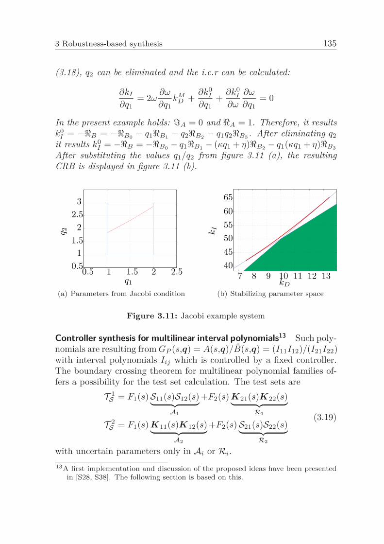
3 Robustness-based synthesis 135
(3.18), q2 can be eliminated and the i.c.r can be calculated:
∂kI
∂q1= 2ω
∂ω
∂q1kM
D +∂k0
I
∂q1+
∂k0I
∂ω
∂ω
∂q1= 0
In the present example holds: �A = 0 and �A = 1. Therefore, it resultsk0
I = −�B = −�B0 − q1�B1 − q2�B2 − q1q2�B3 . After eliminating q2it results k0
I = −�B = −�B0 − q1�B1 − (κq1 + η)�B2 − q1(κq1 + η)�B3
After substituting the values q1/q2 from figure 3.11 (a), the resultingCRB is displayed in figure 3.11 (b).
0.5 1.51 2
10.5
1.52
2.53
2.5q1
q 2
(a) Parameters from Jacobi conditionkD
kI
404550556065
7 8 9 10 11 12 13
(b) Stabilizing parameter space
Figure 3.11: Jacobi example system
Controller synthesis for multilinear interval polynomials13 Such poly-nomials are resulting from GP (s,q) = A(s,q)/B(s,q) = (I11I12)/(I21I22)with interval polynomials Iij which is controlled by a fixed controller.The boundary crossing theorem for multilinear polynomial families of-fers a possibility for the test set calculation. The test sets are
T 1S = F1(s)S11(s)S12(s)︸ ︷︷ ︸
A1
+F2(s) K21(s)K22(s)︸ ︷︷ ︸R1
T 2S = F1(s) K11(s)K12(s)︸ ︷︷ ︸
A2
+F2(s)S21(s)S22(s)︸ ︷︷ ︸R2
(3.19)
with uncertain parameters only in Ai or Ri.13A first implementation and discussion of the proposed ideas have been presented
in [S28, S38]. The following section is based on this.
136 3.2 Test set-based robust controller synthesis
3.2.4 Quasi-polynomials with uncertaintiesTest set theory The Kharitonov theorem is not applicable in the de-lay case as has been demonstrated using an illustrating example in [5].In case of PID control, the term B(s)e τ s includes complex coefficients.The Kharitonov theorem can be extended to the case of complex co-efficients, as presented in [44]. Therefore, the test set contains eightworst-case polynomials. However, the real and the imaginary part ofthe coefficients are still not independent (even for the case of an intervalpolynomial B(s)). Accordingly, the Kharitonov theorem is not applica-ble for quasi-polynomials [110].This phenomenon can also be studied by using the CRB equation for k0
I
in section 2.3.2. This equation shows that the extreme values of k0I are
not correlated with the min/max value of the time delay τ (vertexes ofthe Q-box) because of the trigonometric functions. Hence, in this caseit is not sufficient to test only the vertexes of the Q-box.Test set calculations for time delay systems has extensively been stud-ied in the literature. Several test sets are based on the vertex and edgepolynomials for interval quasi-polynomials. A detailed overview is givenin [72]. Unfortunately, the number of edges which have to be consideredis really big. Therefore, the problem becomes a NP problem [342].In conclusion, for low order delay systems with only interval parameteruncertainty, simple test sets can be calculated and the method presentedin section 3.2.2 can be directly applied to calculate the robust stabilizingparameter space. For high order systems or more advanced uncertaintyrepresentations, alternative methods have to be used as demonstratedin the following.
Optimization-based boundary over-approximation14 This approachis based on a conservative study of the root boundary movement ofthe classical PSA for single-loop LTI systems which are controlled bya PID controller. This approach studied how the root boundaries doshift when the plant parameters vary. Therefore, the challenge which isto guarantee robust stability can be converted into a simple min/maxestimation to calculate the borders of the of root boundary bands. TheRRB and IRBs can be obtained in a similar manar as introduced insection 3.2.2.14The key ideas of this section were published during the project AB 65/2-3 in [275].
3 Robustness-based synthesis 137
In the case of the CRB calculation with parameter uncertainties, thezeros ωS of equation (2.13) can be shifted (see section 2.3.2). Hence,intervals of each zero ωS,t are resulting. Thereby, a CRB band resultsfor each interval. The overall idea of the CRB worst case estimationis to find the borders of the CRB bands with respect to the parameteruncertainty. First, an estimation of the min/max slope (ω2
S,t) of eachCRB band (for every zero ωS interval) with respect to the uncertaintyis performed. The optimization problem is minq∈Q / maxq∈Q ωS,t s.t.equation (2.13). It can be seen that this problem is not convex. Nu-meric tools cannot guarantee to find the global optimum. Consequently,an approach which guarantees the convergence to the global optimummust be developed. The starting point of this approach is to convertthe zero search of equation (2.13) to a min/max search of the kP (ω)function. Using the addition theorems, the k0
I equation in section 2.3.2and equation (2.13) can be modified to a more convenient form:
k0I,t(ωS,t) = sgn(�B)
√�2
B + �2B
�A︸ ︷︷ ︸α
sin
⎛⎜⎜⎜⎜⎝ωS,tτ + arctan(
�B
�B
)︸ ︷︷ ︸
β
⎞⎟⎟⎟⎟⎠+ ωS,tkP �A
�A︸ ︷︷ ︸κ
and 0 = sgn(�B)
√�2
B + �2B
ω2(�2
A + �2A
)︸ ︷︷ ︸ζ
sin
⎛⎜⎜⎜⎝ωτ + arctan(
f2
f1
)︸ ︷︷ ︸
ε
⎞⎟⎟⎟⎠︸ ︷︷ ︸
h(ω,q)
−kP
with f1 = �A�B + �A�B and f2 = �A�B − �A�B .
One possible way to guarantee stability of the resulting PID parameterspace (without convergence problems) is an overestimation of the sec-ond equation. The idea is to analyze all terms in the previous equationseparately. The time delay τ has the strongest influence on ωS becausethe frequency change is mainly based on the time delay variation Δτ , seefigure 3.13. The value of the time delay in order to minimize/maximizeh(ω) is known exactly. The resulting values of τmin/τmax correspond tohmin(ωS)/hmax(ωS) and lead to the min/max ωS,t. Hence, it can beassumed that uncertainty in the time delay does not produce conser-
138 3.2 Test set-based robust controller synthesis
vatism. The term ε changes the frequency of h(ωS). It is easy to seethat ε becomes maximal when f1 is minimal and f2 maximal. An in-crease in ζ causes a growth of the amplitude of h(ωS) and the zerosωS are shifting outwards. The largest amplitude results in the largestabsolute value of �A and �B as well as in the smallest possible absolutevalue of �A and �A. Hence, every real and imaginary part in the twoequations above has to be optimized separately. Therefore, the small-est/largest zero can easily be calculated because now all variables areinterpreted independently. The decoupled analysis leads to a neglectingof the coupled dependency of the real and imaginary parts. Accordingly,the solution is conservative. The conservatism grows with the value ofthe uncertainties in the A(s) and B(s) polynomial.One method to reduce the conservatism without losing the guaranteeof robust stability of the whole resulting PID area is to use a numericalcalculation of the rightmost eigenvalue of the system in every cornerof the previously calculated PID parameter space. The PID parameterspace is limited by the root boundaries where the closed system eigen-value is zero. Hence, the corners of the PID parameter space can beadapted until the rightmost eigenvalue in each corner is equal to zero.The adaption can be realized as demonstrated in [205].Based on the min/max ωS,t of each zero ωS interval and the parameteruncertainty, an estimation of the min/max which corresponds to theintersection point (k0
I,t) of each CRB band can be performed. This canbe done easily because τ and ε are only affecting the frequency of thesinus term. Hence, in the first step the amplitude α and the linear termκ are minimized/maximized. In the second step, τ and ε which min/-max the individual k0
I,i are found using a simple parameter variation.By using this calculation scheme, it is assumed that the bounds (min/-max ωS,t) of each zero ωS interval generate the min/max k0
I,t. But thisis not generally fulfilled and generates an overestimation of the CRBbands. The maximum error which occurs (shift of the CRB) corre-sponds to the maximum amount of k0
I,t. The amount of k0I,t is propor-
tional to the amount of ωS,t. In the time delay case, the amount of ωS,t
is directly growing with the amount of uncertainty in the delay τ .
Example 3.6. Consider the HODF system with a additional delay of0.75 seconds and a ±10% uncertainty in all system parameters and inthe time delay. During the following calculation a constant k∗
P = 1 is
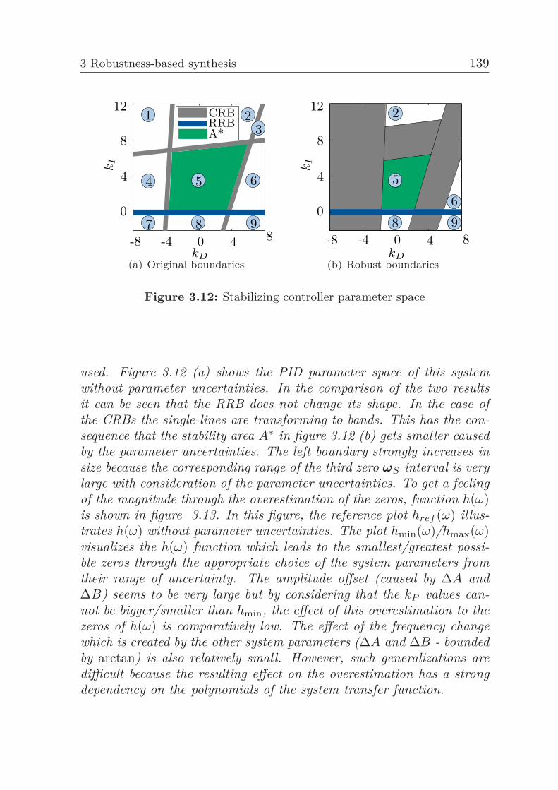
3 Robustness-based synthesis 139
0 4 8-4-8
0
4
8
12k
I
kD
1
4
7 8
5 6
32
9
CRBRRBA*
(a) Original boundaries
0 4 8-4-8
0
4
8
12
kI
kD
1
4
7 8
5 6
32
9
CRBsRRBA*
56
8 9
2
(b) Robust boundaries
Figure 3.12: Stabilizing controller parameter space
used. Figure 3.12 (a) shows the PID parameter space of this systemwithout parameter uncertainties. In the comparison of the two resultsit can be seen that the RRB does not change its shape. In the case ofthe CRBs the single-lines are transforming to bands. This has the con-sequence that the stability area A∗ in figure 3.12 (b) gets smaller causedby the parameter uncertainties. The left boundary strongly increases insize because the corresponding range of the third zero ωS interval is verylarge with consideration of the parameter uncertainties. To get a feelingof the magnitude through the overestimation of the zeros, function h(ω)is shown in figure 3.13. In this figure, the reference plot href (ω) illus-trates h(ω) without parameter uncertainties. The plot hmin(ω)/hmax(ω)visualizes the h(ω) function which leads to the smallest/greatest possi-ble zeros through the appropriate choice of the system parameters fromtheir range of uncertainty. The amplitude offset (caused by ΔA andΔB) seems to be very large but by considering that the kP values can-not be bigger/smaller than hmin, the effect of this overestimation to thezeros of h(ω) is comparatively low. The effect of the frequency changewhich is created by the other system parameters (ΔA and ΔB - boundedby arctan) is also relatively small. However, such generalizations aredifficult because the resulting effect on the overestimation has a strongdependency on the polynomials of the system transfer function.
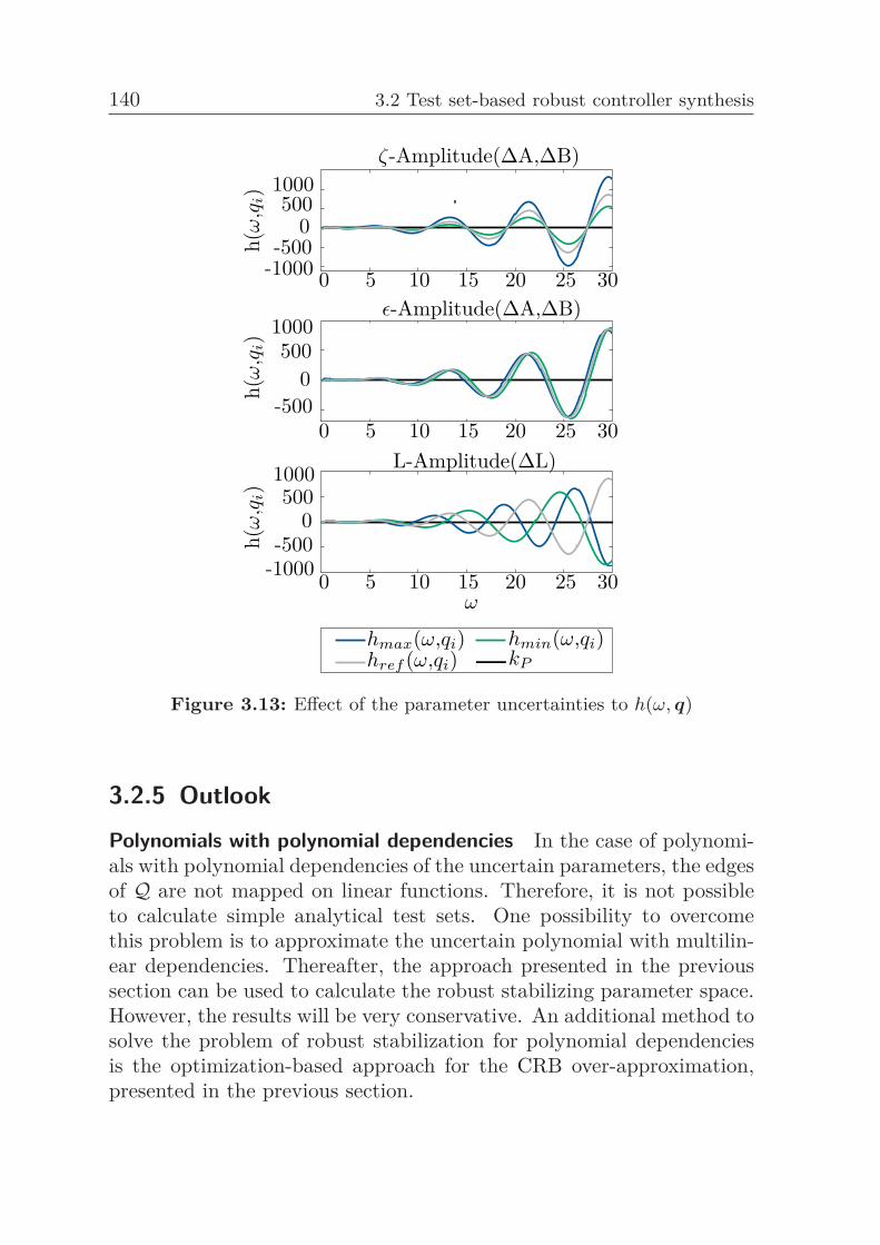
140 3.2 Test set-based robust controller synthesis
ζ-Amplitude(ΔA,ΔB)
ε-Amplitude(ΔA,ΔB)
L-Amplitude(ΔL)
ω
h(ω
,qi) 1000
5000
-500-1000 0 5 10 15 20 25 30
1000500
0-500
1000500
0-500
-1000
h(ω
,qi)
h(ω
,qi)
0 5 10 15 20 25 30
0 5 10 15 20 25 30
hmin(ω,qi)kP
hmax(ω,qi)href (ω,qi)
Figure 3.13: Effect of the parameter uncertainties to h(ω, q)
3.2.5 OutlookPolynomials with polynomial dependencies In the case of polynomi-als with polynomial dependencies of the uncertain parameters, the edgesof Q are not mapped on linear functions. Therefore, it is not possibleto calculate simple analytical test sets. One possibility to overcomethis problem is to approximate the uncertain polynomial with multilin-ear dependencies. Thereafter, the approach presented in the previoussection can be used to calculate the robust stabilizing parameter space.However, the results will be very conservative. An additional method tosolve the problem of robust stabilization for polynomial dependenciesis the optimization-based approach for the CRB over-approximation,presented in the previous section.
3 Robustness-based synthesis 141
Mixed parameter space calculation15 One additional approach is togrid the controller parameter space and calculate the distance of theoperating domain Q to the stability boundary for each point in thesystem parameter space. If the distance is positive the controller pa-rameter set is robust stable. Based on this, the robust stabilizing con-troller parameter can be easily detected. This idea is a bit similar tothe forward/backward scheme for the over-approximation quantificationof interval arithmetic methods [195, 300]. Unfortunately, the computa-tional effort increases rapidly for high dimensional problems and smallinsulated instability regions can be missed. A computational methodbased on this idea has been implemented in [59]. Actually, this methodcan deal only with very low order problems because it needs frequencysweeping during the PSA-based robust stability region calculation pro-cedure, see section 4.2.A similar but much more efficient idea would be the use of the Lyapunovstability-based stability region calculation method, proposed in section2.6. Therefore, the parameter region consisting of the controller as wellthe uncertain system parameters can be calculated. The resulting sta-bility region has to be projected to the controller parameter space to getthe robust stabilizing parameter set. In the same way, the probabilisticstability calculation method can be used. This method has the advan-tages that it is applicable for more general system classes. However,it cannot guarantee that all small isolated instability regions are foundbut the resulting parameter space will be less conservative in compari-son to the previously mentioned over-approximation. This idea is alsoapplicable in the case of polynomials with multilinear dependencies. Byusing the introduced methods in section 3.2.3, the test set will be reallybig and the resulting parameter space will be conservative.The application of the probabilistic stability calculation can reduce theconservatism in this case. Additionally, the a-priori know-ledge aboutthe test set can speed up the calculations. Therefore, the griding pointscan be directly spread into regions where the boundaries of the test setare expected.
15The key ideas of this section were published during the project AB 65/2-3 in [250].16A first implementation and discussion of the proposed ideas have been presented
in [S43]. The following section is based on this.
142 3.2 Test set-based robust controller synthesis
Test set-based Lyapunov stability mapping approach16 In additionto the previously presented classical test set-based PSA method, theLyapunov stability-based mapping method can be directly used, intro-duced in section 2.6. A classical result is to model the system as a systemwith interval uncertainties and check the Lyapunov stability conditionfor each worst case system by taking into consideration that a commonP matrix has to be used. This is similar to the case of the switchingsystems. An alternative possibility is to use the parameter-dependentLyapunov function [112]. For a system of the form
x = A(q) x =
⎛⎝A +h∑
i=1qiAi
⎞⎠x,
the system dynamic can be composed in a sum of independent sub-dynamics with interval uncertainties qi ∈ [q−
i , q+i ]. The previous men-
tioned use of a common Lyapunov function which guarantees the sta-bility of all system parameter combinations gives conservative results.Therefore, a parameter depending Lyapunov function V (x) = xT P (q)xwith
P (q) = P +h∑
i=1qiP i
can be used. The following conditions has to be checked to guaranteerobust stability [113]:
ATi P i + P iAi � 0 with i = 1, 2, . . . , h
andA(Qki)T P (Qki) + P (Qki)A(Qki) ≺ 0.
The set Qki includes all edges of the operating domain qi ∈ {q−i , q+
i }.Moreover, it has to be guaranteed that the center point qi = 1
2 (q−i +q+
i )is stable. Finally, h+2h+1 independent LMIs result. The computationaleffort grows exponentially with the number of uncertain parameters.After mapping the LMIs into the parameter space, the intersection areaof all resulting stability boundaries is the robust stable parameter set.Therefore, the same trade-off between conservatism and computationalcomplexity results, like already discussed before. Also time varying
3 Robustness-based synthesis 143
systems can be analyzed with a similar method [113]. A further researchtopic regarding the robust stability test with Lyapunov functions couldbe a detailed study of perturbed systems based on the eigenvalues andspectral abscissa of P and Q, as started in [334].
Robust Min-Max MPC Today a popular control method is the Min-Max MPC. The main idea behind this method is to proceed a worstcase optimization in order to find, within each time step, the controlleroutput which optimizes a predefined cost function under considerationof the system uncertainties. For a survey about Min-Max MPC, see e.g.[236]. Most often this approach provides conservative results becausethe worst case optimization is mostly restricted to simple uncertaintymodels. Furthermore, it uses only simple test sets, like in section 3.2.1.Therefore, the ideas discussed in section 3.2 can be used to create moresuitable test sets to guarantee robust stability and reduce the conser-vatism. To use results for the robust MPC, they have to be extendedfor the case of discrete time systems, as started in [344]. Regarding thisit could also be interesting to study LMI-based MPCs. By applying theresult of section 2.6, the LMIs can be mapped into the stability region.This offers a more detailed understanding of the optimization problemand helps to study the stability and robustness of this system. Dueto the calculation effort for the stability boundary calculation of highorder systems, the parameter space-based study will not offer a way tospeed up the on-line solver in order to find optimal parameter gains.
3.3 LTV system stability-based approachIf it is known how the parameters of the system change over time, asystem can be modeled as a linear time-variant (LTV) system. Thestability analysis of LTV systems is challenging. Consequently, the dy-namics of such systems are often over-approximated and analyzed byusing LTI robust control techniques, as presented in section 3.2. Unfor-tunately, these results are often very conservative. Therefore, stabilityregion calculation methods which explicitly consider the LTV dynamicsare discussed in the following section. The state space representationof LTV systems is x(t) = A(t)x(t) + B(t)u(t) with y(t) = C(t)x(t).The state transition matrix is defined as the matrix whose productwith the state vector x at an initial time t0 gives x at a later time t:
144 3.3 LTV system stability-based approach
x(t) = Φ(t,t0)x(t0). It can also be used to obtain the general solutionof linear dynamical systems. For LTV systems, Φ(t,t0) is often very dif-ficult to obtain. However, several formulations do exist to find Φ(t,t0)for LTV systems. The calculation of Φ(t,t0) for several classes of LTVsystems have been presented in [163,333]. In [334], an interesting studyof differential sensitivity of Φ(t,t0) is presented.
Frozen time eigenvalues The Frozen time eigenvalues (FTEs) wereproven to be ineffective regarding their contradiction with the system’sstate transition matrix Φ(t,t0), see e.g. [353]. Consequently, the FTEscannot be used for the analysis of the stability of general LTV systems.One special LTV system class which can be studied by applying theFTEs are the slowly varying systems. To check if a system is slowlyvarying, it has to be proven that the norm of A(t) is bounded for allvalues of t and the change of the parameters of A(t) is also sufficientlysmall. For detailed information see e.g. classical papers like [299].Parameter regions can be calculated for slowly varying systems by usingthe FTEs. In a first step the characteristic equation and the stabilityboundaries (RRB, CRB and IRB) have to be calculated as a functionof t. A whole range of stability boundaries with an infinite number oflines results because they are a function of t. In a next step a worst-case study has to be carried out to calculate the extreme positions of theboundaries (e.g. for the RRB: which is the biggest and smallest valueof k1, which is included in the RRB). After this has been completed thestability boundary zones can be plotted. With the condition that thenorm of A(t) is bounded for all values of t it can easily be concludedthat also the resulting sets of stability boundaries are bounded.An additional frozen time eigenvalue-based stability region calculationmethod could be a common Lyapunov matrix-based stability test. Acommon as well as a more sophisticated Lyapunov stability-based studyof LTV systems have been presented in [355]. This method is too con-servative respectively too complex to merge it easily with the resultspresented in section 2.6.
17A first implementation and discussion of the proposed ideas have been presentedin [S15]. The following section is based on this. The key ideas of this sectionwere published during the project AB 65/2-3 in [269].
3 Robustness-based synthesis 145
Dynamic eigenvalue-based approach17 A lot of research was per-formed over the past 30 years to develop eigenvalue-based LTV stabilityapproaches: extended eigenvalues and eigenvectors concept [341], rightpoles [169], D-eigenvalues [354], dynamic eigenvalues and eigenvectors[84–86]. The concept of dynamic eigenvalues is considered in the fol-lowing. The other approaches have a similar main idea. The theorydeveloped by P. Van der Kloet and F. L. Neerhoff aimed to formulatethe general solution of nth order homogeneous LTV systems. This wasdone by decoupling the LTV system into n different LTV systems of thefirst order via coordinate transformation where each of the first ordersystems gets the general form xt(t) = λ(t)xt(t) where xt is a new statevariable related to the state variables of the original LTV system andλ(t) is the dynamic eigenvalue. Each of these scalar systems can besolved easily when using the dynamic eigenvalues.It was determined that considering the dynamic eigenvalues as quan-tities similar to the eigenvalues of LTI systems which wander in timethrough the complex s-domain is a common misconception and the pro-posed method failed. This conclusion is a result of the work [132]. M. A.Gutierrez de Anda presented an overview of the relation between the dy-namic eigenvalues and the frequency domain. He has shown that thereis no link between the dynamic eigenvalue concept and the s-domain.Hence, the dynamic eigenvalue-based PSA failed.
Transformation of LTV to LTI systems18 The analysis and synthesisof LTI systems is quite developed. However, general transparent meth-ods for the analysis of the stability of LTV systems are still lacking, asshown before. Therefore, if a LTV system can be transformed into aLTI system, then the transparent results for time-varying systems canbe obtained. According to [340] any LTV system can be transformedinto an equivalent LTI system, provided that the state transition matrixΦ(t,t0) is known. Since [340] was published back in the 1970s a genericmethod was not illustrated due to the difficulty in obtaining Φ(t,t0) forLTV systems. Hence, the author explained explicit methods in order toobtain the transformation for special classes of LTV systems. Throughresearch about the calculation of the Φ(t,t0) for LTV systems in the
18A first implementation and discussion of the proposed ideas have been presentedin [S15]. The following section is based on this. The key ideas of this sectionwere published during the project AB 65/2-3 in [269].
146 3.3 LTV system stability-based approach
past 30 years, the results can be utilized with the following method inorder to find a general transformation criterion for more classes of LTVsystems.A LTV system x = A(t)x is invariable if it can be transformed intoa LTI system of the form ˙x = Ax by some valid transformation suchas the algebraic transformation and the t ↔ τ transformation. Analgebraic transformation is a transformation of the states defined byx(t) = T (t)x(t) where T (t) is a non-singular matrix for all t (matrixT (t) has an inverse) and T (t) exists. Moreover, a t↔ τ transformationis a transformation of time scale from t into τ . Based on the corollariesand their corresponding examples presented in [340], the idea of trans-forming the LTV system into its equivalent LTI system is followed byapplying the PSA. A fundamental improvement of this method couldbe research based on finding a generic method for the transformationof any LTV system into its equivalent LTI system. As has been pointedout in [340], this is possible if the state transition matrix Φ(t,t0) of theLTV system is known. However, a clear method for deriving the alge-braic transformation matrix T (t) by using Φ(t,t0) for any generic casewas not illustrated by M. Wu in [340] due to the difficulty in obtainingthe state transition matrices of LTV systems back in the 1970s.
Example 3.7. Consider the algebraic invariable LTV system
A(t) =[−5 + cos(ωt) sin(ωt)− sin(ωt) −5 + cos(ωt)
].
A(t) is a commutative system because it holds
A(t)
⎡⎢⎣ t∫t0
A(τ)dτ
⎤⎥⎦ =
⎡⎢⎣ t∫t0
A(τ)dτ
⎤⎥⎦A(t).
A detailed definition of commutative algebraic invariable LTV systemsgiven in [340]. The matrix A(t) can be rewritten as
A(t) = cos(ωt)︸ ︷︷ ︸α1(t)
[1 00 1
]︸ ︷︷ ︸
F1
+ sin(ωt)︸ ︷︷ ︸α2(t)
[0 1−1 0
]︸ ︷︷ ︸
F2
+[−5 00 −5
]︸ ︷︷ ︸
G
.
3 Robustness-based synthesis 147
The following transformation steps are completely based on [340]. There-fore, the transformation is presented only in a very short way. Basedon matrix A(t) the following transformation matrix is chosen
T (t) = exp[[
1 00 1
]β1(t) +
[0 1−1 0
]β2(t)
]= exp
[β1(t) β2(t)−β2(t) β1(t)
]with
β1(t) =1∫
0
cos(ωt) =1ω
sin(ωt) and β2(t) =1∫
0
sin(ωt) =1ω
(1− cos(ωt)).
By using the exponential matrix calculation rule
exp[M ] =∞∑
n=0
Mn
n!= I + M +
MM
2!+
MMM
3!+ · · ·
where I is the identity matrix, the transformation matrix is given as
T (t) = exp[β1(t)][
cos(β2(t)) sin(β2(t))− sin(β2(t)) cos(β2(t))
].
Applying A = T −1(t)A(t)T (t)−T −1(t)T (t) to the example system, theLTI system results
˙x(t) =[−5 00 −5
]︸ ︷︷ ︸
A=G
x(t).
To calculate the stabilizing parameter space of the LTV system, thecharacteristic equation of the equivalent LTI system is used δ(s,k) =s2 + (10 + k2)s + (25 + 5 k2) = 0. This is k2 = −5 for the RRB. ACRB and IRB do not exist. Based on the state transition matrix orsimulations it can be shown that the RRB is correct. If any k1 and k2equal to −5 is used, the system response shows a permanent oscillationbecause it is on the stability margin. If any value in the stable param-eter space is taken, the closed-loop step response of the LTV systemis stable. For any parameter outside the stable area the step responsegoes to infinity. Hence, it is unstable. Comparing the resulting con-troller parameter spaces of the LTV/LTI-transformation approach withthe results of a LTI-overestimation in the sense of interval polynomi-
148 3.4 Robustness verification techniques
als with α1 = [−4,−6] and α2 = [−1, 1]. it is obvious that the LTI-overestimation approach is much more conservative. The conservatismof this approach is easy to see if the RRB equation is analyzed. For thepoint α1 = −4 and α2 = 0 inside the operation domain, the RRB getsk2 = −4 . The real boundary is k2 = −5. As a consequence the stabil-ity area shrinks through the use LTI overestimation in contrast to theLTV/LTI-transformation. Additional examples are presented in [269].
3.4 Robustness verification techniquesIn the following section, graphical techniques in order to validate andverify the robustness of a chosen controller are discussed.
Verification-based on Tsypkin plots19 In [316], Y. Z. Tsypkin estab-lished a criterion for the stability of time delay systems, based on theopen-loop transfer function G0(jω) = G(jω)e j[ξ(ω)−τω]. The system ison the stability margin if G(jω) = 1 and Ξ(ω)− τω = −2πr as well asG(jω) = −1 and Ξ(ω) − τω = −2πr + π. The stability critical delayis the first one which fulfills this conditions. Therefore, the Tsypkincondition which determine the maximum time delay value is:
τmax = minω ∈ Ω
Ξ(ω)ω
(3.20)
where Ω is the set of critical frequencies at which the Nyquist plotof the transfer function crosses the unit circle and Ξ(ω) is the anglefrom the intersection points on the Nyquist plot to the negative realaxis. In the following, a method that shows how the maximum timedelay behaves in relation to the uncertainty in the gain is developed.Therefore, the values of the maximum allowable time delay of eachfrequency in the interval of the gain uncertainty bounds are plotted,similar to the methods discussed in section 2.5.1. The estimation ofthe maximum allowable time delay is based on [317]. This method wasinspired by the Hansen plot analysis presented in [119, 137] where theNyquist-based stability condition is mapped to the system parameters.In figure 3.14, the modified Tsypkin plot shows how many uncertaintiesin the gain and time delay can be tolerated by a second order timedelay system. The plotted circles represent the system gain uncertainty19A first implementation and discussion of the proposed ideas have been presented
in [S19]. The following section is based on this.
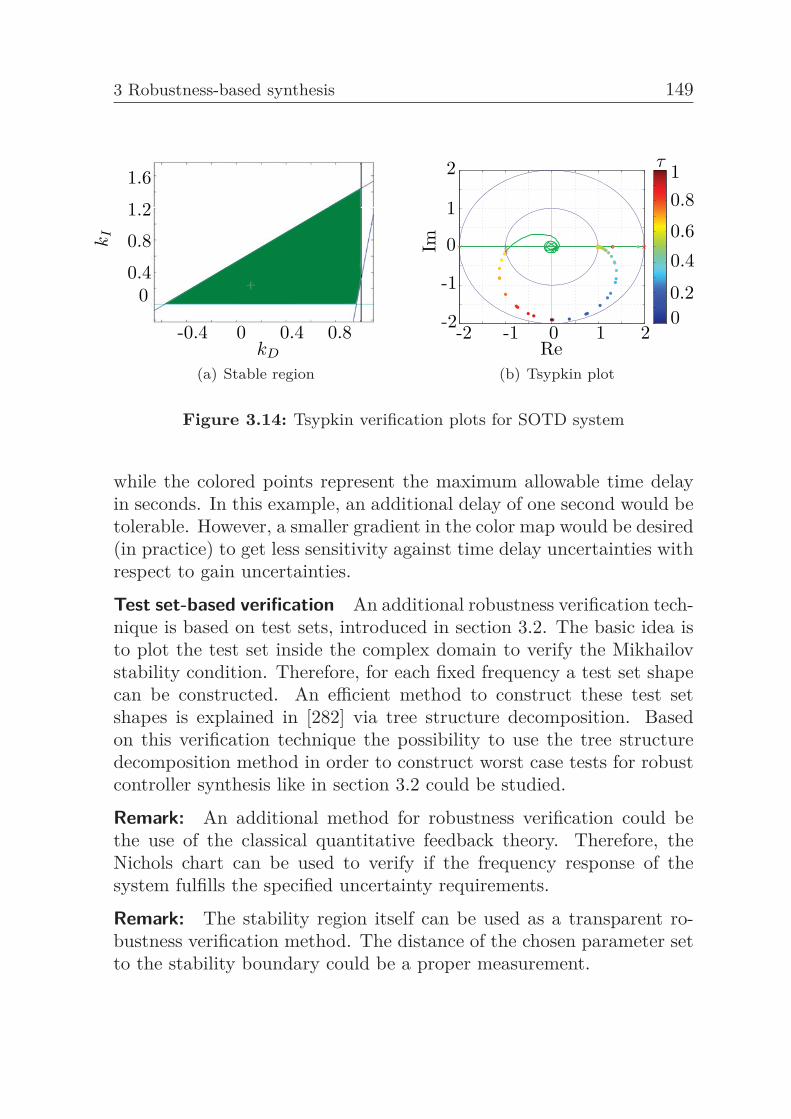
3 Robustness-based synthesis 149
kD
kI
00.4
0.8
1.2
1.6
0-0.4 0.4 0.8
(a) Stable regionRe
Im 0
-1
-2-2 -1 0 1 2
0.40.6
0.8
0.20
1
2 1τ
(b) Tsypkin plot
Figure 3.14: Tsypkin verification plots for SOTD system
while the colored points represent the maximum allowable time delayin seconds. In this example, an additional delay of one second would betolerable. However, a smaller gradient in the color map would be desired(in practice) to get less sensitivity against time delay uncertainties withrespect to gain uncertainties.
Test set-based verification An additional robustness verification tech-nique is based on test sets, introduced in section 3.2. The basic idea isto plot the test set inside the complex domain to verify the Mikhailovstability condition. Therefore, for each fixed frequency a test set shapecan be constructed. An efficient method to construct these test setshapes is explained in [282] via tree structure decomposition. Basedon this verification technique the possibility to use the tree structuredecomposition method in order to construct worst case tests for robustcontroller synthesis like in section 3.2 could be studied.
Remark: An additional method for robustness verification could bethe use of the classical quantitative feedback theory. Therefore, theNichols chart can be used to verify if the frequency response of thesystem fulfills the specified uncertainty requirements.
Remark: The stability region itself can be used as a transparent ro-bustness verification method. The distance of the chosen parameter setto the stability boundary could be a proper measurement.
150
4 Performance-based synthesisToday, various approaches for controller performance tuning are avail-able. They are based on quite different tuning objectives in the timeand frequency domain. Important contradictory tuning objectives areperformance versus robustness aspects of controller design [114]. Com-mon tuning approaches are considering only a single criterion. More-over, most of the tuning approaches deal only with time delay approx-imations and ignore parameter uncertainties completely. The goal ofthe presented subsequently assisted or even automatic controller tun-ing method is to guide the controller designer through the stabilizingcontroller parameter space to find the best fitting controller parameterset under consideration of several controller design objectives. This isneeded because in general it is difficult to choose the best fitting con-troller parameter combination of the whole multidimensional parameterspace. The dependency of the controller performance on the location ofthe controller parameter inside the previously calculated stability regionis difficult to comprehend. Therefore, the classical stability region-basedcontroller tuning consists of an unacceptable time consuming iterativesearch. This section shows a stability region-based controller tuningapproach which consists of the following steps:1) Parameter space shrinking: Shrinking the parameter area withconsidering performance and robustness specifications (e.g. minimumgain and phase margins or the results of section 3). The resulting param-eter region shrinks to guarantee predefined performance and robustnesscriteria.2) Color mapping: This step deals with the projection of severaltuning objectives onto two dimensional controller parameter spaces inform of color maps. Therefore, the closed-loop properties of relevantcontroller parameters are projected into the stabilizing controller pa-rameter space. The following study is restricted to 2D performancemaps due to the simplicity of the visualization. By using these maps,the performance and robustness of the parameter candidates can beeasily quantified. This allows an fine adjustment of the controller pa-rameters.
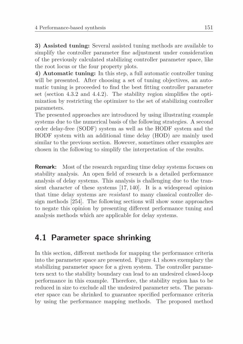
4 Performance-based synthesis 151
3) Assisted tuning: Several assisted tuning methods are available tosimplify the controller parameter fine adjustment under considerationof the previously calculated stabilizing controller parameter space, likethe root locus or the four property plots.4) Automatic tuning: In this step, a full automatic controller tuningwill be presented. After choosing a set of tuning objectives, an auto-matic tuning is proceeded to find the best fitting controller parameterset (section 4.3.2 and 4.4.2). The stability region simplifies the opti-mization by restricting the optimizer to the set of stabilizing controllerparameters.The presented approaches are introduced by using illustrating examplesystems due to the numerical basis of the following strategies. A secondorder delay-free (SODF) system as well as the HODF system and theHODF system with an additional time delay (HOD) are mainly usedsimilar to the previous section. However, sometimes other examples arechosen in the following to simplify the interpretation of the results.
Remark: Most of the research regarding time delay systems focuses onstability analysis. An open field of research is a detailed performanceanalysis of delay systems. This analysis is challenging due to the tran-sient character of these systems [17, 140]. It is a widespread opinionthat time delay systems are resistant to many classical controller de-sign methods [254]. The following sections will show some approachesto negate this opinion by presenting different performance tuning andanalysis methods which are applicable for delay systems.
4.1 Parameter space shrinkingIn this section, different methods for mapping the performance criteriainto the parameter space are presented. Figure 4.1 shows exemplary thestabilizing parameter space for a given system. The controller parame-ters next to the stability boundary can lead to an undesired closed-loopperformance in this example. Therefore, the stability region has to bereduced in size to exclude all the undesired parameter sets. The param-eter space can be shrinked to guarantee specified performance criteriaby using the performance mapping methods. The proposed method
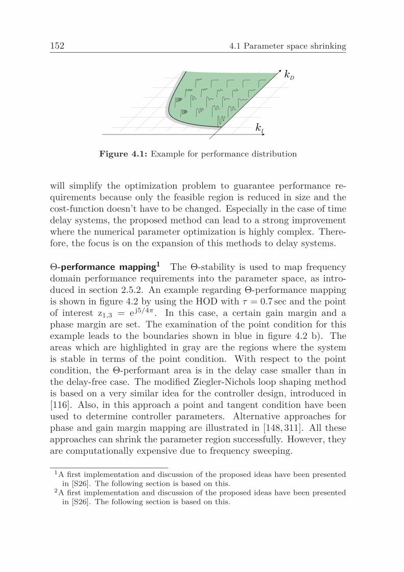
152 4.1 Parameter space shrinking
Figure 4.1: Example for performance distribution
will simplify the optimization problem to guarantee performance re-quirements because only the feasible region is reduced in size and thecost-function doesn’t have to be changed. Especially in the case of timedelay systems, the proposed method can lead to a strong improvementwhere the numerical parameter optimization is highly complex. There-fore, the focus is on the expansion of this methods to delay systems.
Θ-performance mapping1 The Θ-stability is used to map frequencydomain performance requirements into the parameter space, as intro-duced in section 2.5.2. An example regarding Θ-performance mappingis shown in figure 4.2 by using the HOD with τ = 0.7 sec and the pointof interest z1,3 = e j5/4π. In this case, a certain gain margin and aphase margin are set. The examination of the point condition for thisexample leads to the boundaries shown in blue in figure 4.2 b). Theareas which are highlighted in gray are the regions where the systemis stable in terms of the point condition. With respect to the pointcondition, the Θ-performant area is in the delay case smaller than inthe delay-free case. The modified Ziegler-Nichols loop shaping methodis based on a very similar idea for the controller design, introduced in[116]. Also, in this approach a point and tangent condition have beenused to determine controller parameters. Alternative approaches forphase and gain margin mapping are illustrated in [148, 311]. All theseapproaches can shrink the parameter region successfully. However, theyare computationally expensive due to frequency sweeping.
1A first implementation and discussion of the proposed ideas have been presentedin [S26]. The following section is based on this.
2A first implementation and discussion of the proposed ideas have been presentedin [S26]. The following section is based on this.
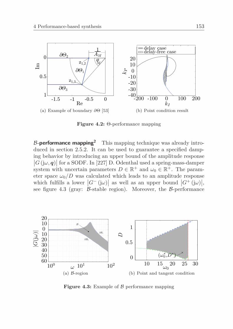
4 Performance-based synthesis 153
(a) Example of boundary ∂Θ [53]
delay casedelay-free case
kP
kI
0 100 200-100-200-40-30-20-10
01020
(b) Point condition result
Figure 4.2: Θ-performance mapping
B-performance mapping2 This mapping technique was already intro-duced in section 2.5.2. It can be used to guarantee a specified damp-ing behavior by introducing an upper bound of the amplitude response∣∣G (jω, q)
∣∣ for a SODF. In [227] D. Odenthal used a spring-mass-dampersystem with uncertain parameters D ∈ R
+ and ω0 ∈ R+. The param-
eter space ω0/D was calculated which leads to an amplitude responsewhich fulfills a lower
∣∣G− (jω)∣∣ as well as an upper bound
∣∣G+ (jω)∣∣,
see figure 4.3 (gray: B-stable region). Moreover, the B-performance
100 101 10260504030201001020
|G(j
ω)|
ω(a) B-region
(ω∗0 ,D∗)
ω0
D
0
0.5
1
10 15 20 25 30
(b) Point and tangent condition
Figure 4.3: Example of B performance mapping
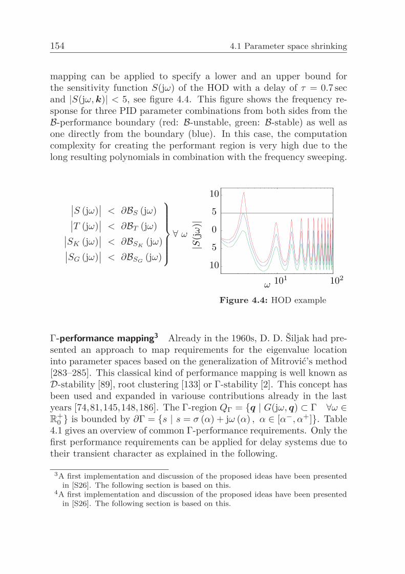
154 4.1 Parameter space shrinking
mapping can be applied to specify a lower and an upper bound forthe sensitivity function S(jω) of the HOD with a delay of τ = 0.7 secand |S(jω, k)| < 5, see figure 4.4. This figure shows the frequency re-sponse for three PID parameter combinations from both sides from theB-performance boundary (red: B-unstable, green: B-stable) as well asone directly from the boundary (blue). In this case, the computationcomplexity for creating the performant region is very high due to thelong resulting polynomials in combination with the frequency sweeping.
∣∣S (jω)∣∣ < ∂BS (jω)∣∣T (jω)∣∣ < ∂BT (jω)∣∣SK (jω)∣∣ < ∂BSK
(jω)∣∣SG (jω)∣∣ < ∂BSG
(jω)
⎫⎪⎪⎪⎪⎪⎬⎪⎪⎪⎪⎪⎭∀ ω
100 101 102
10
5
0
5
10
ω
|S(j
ω)|
Figure 4.4: HOD example
Γ-performance mapping3 Already in the 1960s, D. D. Šiljak had pre-sented an approach to map requirements for the eigenvalue locationinto parameter spaces based on the generalization of Mitrović’s method[283–285]. This classical kind of performance mapping is well known asD-stability [89], root clustering [133] or Γ-stability [2]. This concept hasbeen used and expanded in variouse contributions already in the lastyears [74,81,145,148,186]. The Γ-region QΓ = {q | G(jω, q) ⊂ Γ ∀ω ∈R
+0 } is bounded by ∂Γ = {s | s = σ (α) + jω (α) , α ∈ [α−, α+]}. Table
4.1 gives an overview of common Γ-performance requirements. Only thefirst performance requirements can be applied for delay systems due totheir transient character as explained in the following.
3A first implementation and discussion of the proposed ideas have been presentedin [S26]. The following section is based on this.
4A first implementation and discussion of the proposed ideas have been presentedin [S26]. The following section is based on this.
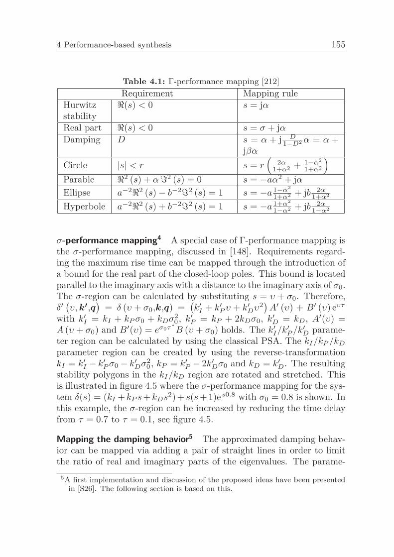
4 Performance-based synthesis 155
Table 4.1: Γ-performance mapping [212]Requirement Mapping rule
Hurwitzstability
�(s) < 0 s = jα
Real part �(s) < 0 s = σ + jαDamping D s = α + j D
1−D2 α = α +jβα
Circle |s| < r s = r(
2α1+α2 + 1−α2
1+α2
)Parable �2 (s) + α�2 (s) = 0 s = −aα2 + jαEllipse a−2�2 (s)− b−2�2 (s) = 1 s = −a 1−α2
1+α2 + jb 2α1+α2
Hyperbole a−2�2 (s) + b−2�2 (s) = 1 s = −a 1+α2
1−α2 + jb 2α1−α2
σ-performance mapping4 A special case of Γ-performance mapping isthe σ-performance mapping, discussed in [148]. Requirements regard-ing the maximum rise time can be mapped through the introduction ofa bound for the real part of the closed-loop poles. This bound is locatedparallel to the imaginary axis with a distance to the imaginary axis of σ0.The σ-region can be calculated by substituting s = υ + σ0. Therefore,δ′ (υ, k′,q
)= δ (υ + σ0,k,q) =
(k′
I + k′P υ + k′
Dυ2)A′ (υ) + B′ (υ) eυτ
with k′I = kI + kP σ0 + kDσ2
0 , k′P = kP + 2kDσ0, k′
D = kD, A′(υ) =A (υ + σ0) and B′(υ) = eσ0τ∗
B (υ + σ0) holds. The k′I/k′
P /k′D parame-
ter region can be calculated by using the classical PSA. The kI/kP /kD
parameter region can be created by using the reverse-transformationkI = k′
I − k′P σ0 − k′
Dσ20 , kP = k′
P − 2k′Dσ0 and kD = k′
D. The resultingstability polygons in the kI/kD region are rotated and stretched. Thisis illustrated in figure 4.5 where the σ-performance mapping for the sys-tem δ(s) = (kI + kP s + kDs2) + s(s + 1)es0.8 with σ0 = 0.8 is shown. Inthis example, the σ-region can be increased by reducing the time delayfrom τ = 0.7 to τ = 0.1, see figure 4.5.
Mapping the damping behavior5 The approximated damping behav-ior can be mapped via adding a pair of straight lines in order to limitthe ratio of real and imaginary parts of the eigenvalues. The parame-
5A first implementation and discussion of the proposed ideas have been presentedin [S26]. The following section is based on this.
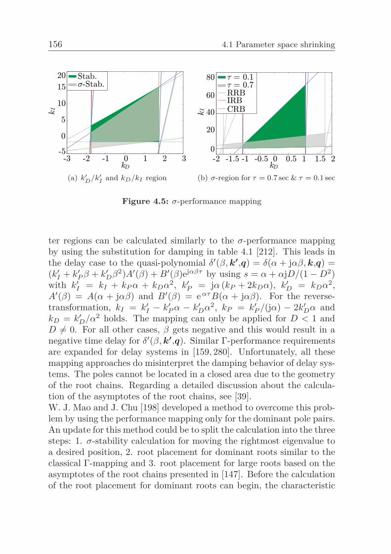
156 4.1 Parameter space shrinking
(a) k′D/k′
I and kD/kI region (b) σ-region for τ = 0.7 sec & τ = 0.1 sec
Figure 4.5: σ-performance mapping
ter regions can be calculated similarly to the σ-performance mappingby using the substitution for damping in table 4.1 [212]. This leads inthe delay case to the quasi-polynomial δ′(β, k′,q) = δ(α + jαβ, k,q) =(k′
I + k′P β + k′
Dβ2)A′(β) + B′(β)ejαβτ by using s = α + αjD/(1−D2)with k′
I = kI + kP α + kDα2, k′P = jα (kP + 2kDα), k′
D = kDα2,A′(β) = A(α + jαβ) and B′(β) = eατ B(α + jαβ). For the reverse-transformation, kI = k′
I − k′P α − k′
Dα2, kP = k′P /(jα) − 2k′
Dα andkD = k′
D/α2 holds. The mapping can only be applied for D < 1 andD �= 0. For all other cases, β gets negative and this would result in anegative time delay for δ′(β, k′,q). Similar Γ-performance requirementsare expanded for delay systems in [159, 280]. Unfortunately, all thesemapping approaches do misinterpret the damping behavior of delay sys-tems. The poles cannot be located in a closed area due to the geometryof the root chains. Regarding a detailed discussion about the calcula-tion of the asymptotes of the root chains, see [39].W. J. Mao and J. Chu [198] developed a method to overcome this prob-lem by using the performance mapping only for the dominant pole pairs.An update for this method could be to split the calculation into the threesteps: 1. σ-stability calculation for moving the rightmost eigenvalue toa desired position, 2. root placement for dominant roots similar to theclassical Γ-mapping and 3. root placement for large roots based on theasymptotes of the root chains presented in [147]. Before the calculationof the root placement for dominant roots can begin, the characteristic
4 Performance-based synthesis 157
equation is needed which only considers the dominant roots. The polescan easily be calculated by using numerical methods like the Lambert-W function or the Arnoldi method (see section 2.1). These methodsneed the specification of the area of interest of the eigenvalue domain inorder to calculate all poles in this area. As soon as this finite number ofpoles has been specified, the characteristic equation can be built up andthe PSA with damping requirements for time delay-free systems can becomputed. Three sets of performance considering parameter spaces re-sult after mapping all these three conditions. The intersection set ofthese three spaces gives the parameter spaces under consideration of allthree Γ-stability requirements.Remark A detailed study of the shape of the resulting parameterspaces after applying the performance transformation could be an in-teresting further research topic. Therefore, a detailed analysis how thestability boundaries are modified by a applying the transformations hasto be done.Iterative controller optimization strategy An iterative optimizationstrategy based on the previously introduced performance mapping meth-ods have been presented in [102]. The closed-loop poles are iterativelyshifted to the left as long as the resulting σ-region is not empty. Unfor-tunately, this tuning method is very computationally expensive.
4.2 Start point calculationA variety of surveys like [81] explore several controller tuning rules tofind a good starting point for the controller fine tuning. In the following,some popular controller tuning methods will be reviewed in order tofind suitable methods for the calculation of the initial controller tuningstarting point which is inside the controller parameter region.
Heuristic PID tuning6 It is a common method to tune the PID con-troller parameters heuristically by using the following rules of thumb.The proportional gain influences the aggressiveness of the closed-loopsystem. An increasing proportional gain reduces the controller error butit can also lead to a bad damping behavior and instability. An integralgain eliminates the controller error. The differential gain increases the
6A first implementation and discussion of the proposed ideas have been presentedin [S40]. The following section is based on this.
158 4.2 Start point calculation
rise time of the closed-loop system but it can produce a bad perfor-mance due to noisy signals [348]. Based on these rules a PID parameterset can be chosen.
Empirical formulas7 It is more efficient to use some standard tuningrules in comparison to the previous try and error method. Many em-pirical formulas for controller tuning exist. The most popular one isthe Ziegler-Nichols method. In the case of dominant time delays, theclosed-loop version of this method does not lead to acceptable perfor-mance. Moreover, only a small stability margin results [225, 289]. Thedynamics are denoted as delay dominant if the delay is at least twotimes larger than the dominant time constant T of the system. Theopen-loop tuning version of the Ziegler-Nichols method is restricted tothe case τ/T < 1 [20,281]. Various modifications of this tuning methodexist. One of the most well known is the tuning rule of Chien, Hronesand Reswich [281]. In this case, the controller tuning goal like set-pointfollowing or disturbance rejection can be directly chosen, see e.g. [20].An additional popular method is the Cohen-Coon method. It was de-veloped 11 years after the Ziegler-Nichols method became famous. Thedifference between them is that the Cohen-Coon method depends di-rectly on the process model and was designed mainly for disturbancerejection. The performance of this tuning rule is a bit better in the pres-ence of time delay, but is also not suitable for dominant time delays.For a survey of empirical tuning formulas, see [229].
Internal model control8 The internal model control (IMC) methodwas developed by M. Morari and E. Zafirion [210]. The IMC controllerconsists of a plant model, a low pass filter and a controller block. Forexample, all these three elements can be summarized to one IMC con-troller with PID structure. Model approximations are often used tosimplify the controller synthesis. The most common approximation ap-proach is the half rule of S. Skogestad in [321] which simplifies thesystem to first or second order. The IMC approach offers possibilitiesin order to consider model uncertainties directly as well as performancerequirements for the closed-loop system [281]. A PID controller can be
7A first implementation and discussion of the proposed ideas have been presentedin [S40]. The following section is based on this.
8A first implementation and discussion of the proposed ideas have been presentedin [S40]. The following section is based on this.
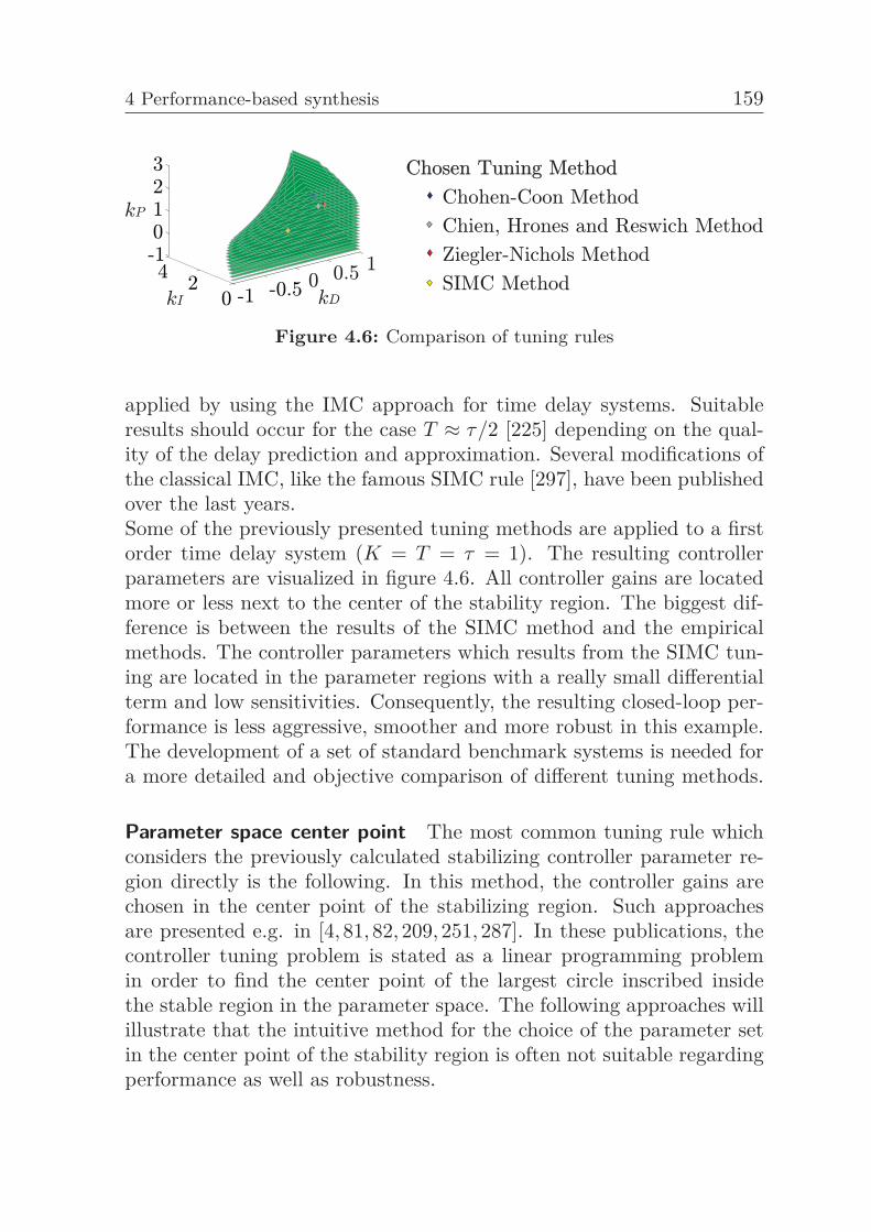
4 Performance-based synthesis 159
Figure 4.6: Comparison of tuning rules
applied by using the IMC approach for time delay systems. Suitableresults should occur for the case T ≈ τ/2 [225] depending on the qual-ity of the delay prediction and approximation. Several modifications ofthe classical IMC, like the famous SIMC rule [297], have been publishedover the last years.Some of the previously presented tuning methods are applied to a firstorder time delay system (K = T = τ = 1). The resulting controllerparameters are visualized in figure 4.6. All controller gains are locatedmore or less next to the center of the stability region. The biggest dif-ference is between the results of the SIMC method and the empiricalmethods. The controller parameters which results from the SIMC tun-ing are located in the parameter regions with a really small differentialterm and low sensitivities. Consequently, the resulting closed-loop per-formance is less aggressive, smoother and more robust in this example.The development of a set of standard benchmark systems is needed fora more detailed and objective comparison of different tuning methods.
Parameter space center point The most common tuning rule whichconsiders the previously calculated stabilizing controller parameter re-gion directly is the following. In this method, the controller gains arechosen in the center point of the stabilizing region. Such approachesare presented e.g. in [4, 81, 82, 209, 251, 287]. In these publications, thecontroller tuning problem is stated as a linear programming problemin order to find the center point of the largest circle inscribed insidethe stable region in the parameter space. The following approaches willillustrate that the intuitive method for the choice of the parameter setin the center point of the stability region is often not suitable regardingperformance as well as robustness.
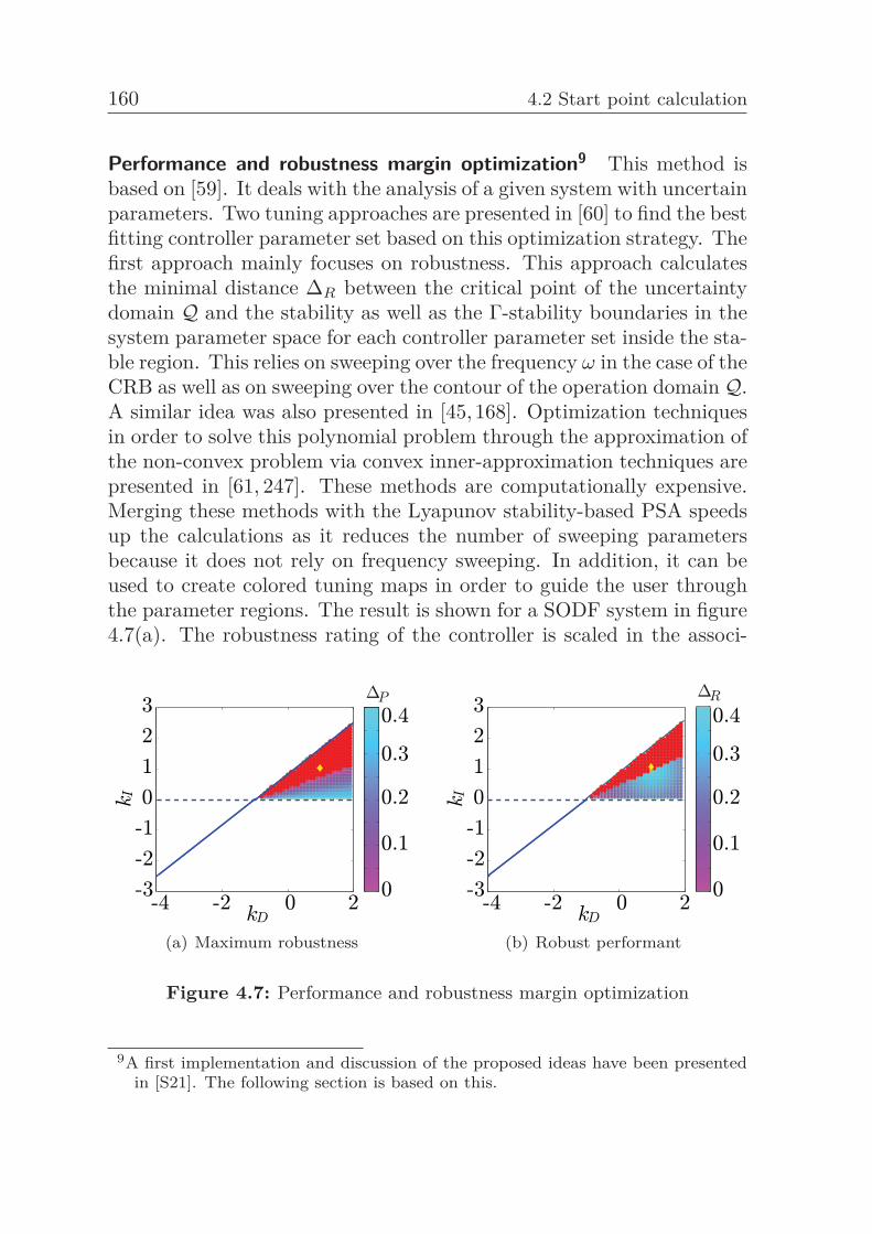
160 4.2 Start point calculation
Performance and robustness margin optimization9 This method isbased on [59]. It deals with the analysis of a given system with uncertainparameters. Two tuning approaches are presented in [60] to find the bestfitting controller parameter set based on this optimization strategy. Thefirst approach mainly focuses on robustness. This approach calculatesthe minimal distance ΔR between the critical point of the uncertaintydomain Q and the stability as well as the Γ-stability boundaries in thesystem parameter space for each controller parameter set inside the sta-ble region. This relies on sweeping over the frequency ω in the case of theCRB as well as on sweeping over the contour of the operation domain Q.A similar idea was also presented in [45, 168]. Optimization techniquesin order to solve this polynomial problem through the approximation ofthe non-convex problem via convex inner-approximation techniques arepresented in [61, 247]. These methods are computationally expensive.Merging these methods with the Lyapunov stability-based PSA speedsup the calculations as it reduces the number of sweeping parametersbecause it does not rely on frequency sweeping. In addition, it can beused to create colored tuning maps in order to guide the user throughthe parameter regions. The result is shown for a SODF system in figure4.7(a). The robustness rating of the controller is scaled in the associ-
(a) Maximum robustness (b) Robust performant
Figure 4.7: Performance and robustness margin optimization
9A first implementation and discussion of the proposed ideas have been presentedin [S21]. The following section is based on this.
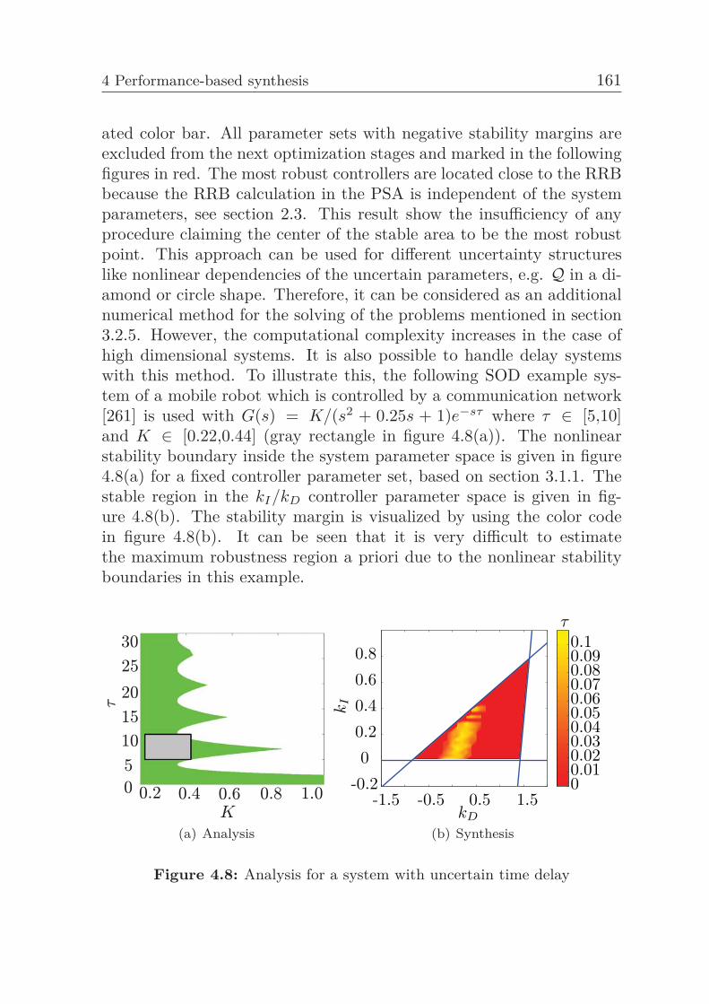
4 Performance-based synthesis 161
ated color bar. All parameter sets with negative stability margins areexcluded from the next optimization stages and marked in the followingfigures in red. The most robust controllers are located close to the RRBbecause the RRB calculation in the PSA is independent of the systemparameters, see section 2.3. This result show the insufficiency of anyprocedure claiming the center of the stable area to be the most robustpoint. This approach can be used for different uncertainty structureslike nonlinear dependencies of the uncertain parameters, e.g. Q in a di-amond or circle shape. Therefore, it can be considered as an additionalnumerical method for the solving of the problems mentioned in section3.2.5. However, the computational complexity increases in the case ofhigh dimensional systems. It is also possible to handle delay systemswith this method. To illustrate this, the following SOD example sys-tem of a mobile robot which is controlled by a communication network[261] is used with G(s) = K/(s2 + 0.25s + 1)e−sτ where τ ∈ [5,10]and K ∈ [0.22,0.44] (gray rectangle in figure 4.8(a)). The nonlinearstability boundary inside the system parameter space is given in figure4.8(a) for a fixed controller parameter set, based on section 3.1.1. Thestable region in the kI/kD controller parameter space is given in fig-ure 4.8(b). The stability margin is visualized by using the color codein figure 4.8(b). It can be seen that it is very difficult to estimatethe maximum robustness region a priori due to the nonlinear stabilityboundaries in this example.
(a) Analysis
-1.5 -0.5 0.5 1.5-0.2
00.20.40.60.8
kI
kD
00.010.020.030.040.050.060.070.080.090.1
τ
(b) Synthesis
Figure 4.8: Analysis for a system with uncertain time delay
162 4.3 Time domain-based optimization
The second tuning approach which was mentioned in [60] considers akind of robust pole assignment. Assuming that the nominal controllersatisfies the desired performance conditions the optimal controller pa-rameter set should be as close as possible to the nominal controller(yellow marker in figure 4.7 (b)) by guarantying robustness. There-fore, the previously presented method can be used directly. Only thecost-function to create the color map has to be changed to the minimaldistance ΔP between the nominal controller and a robust controller, seefigure 4.7(b). A similar method was already proposed by [334].
4.3 Time domain-based optimizationIn this section, different methods for time domain-based controller op-timization methods are presented. The controller tuning in the timedomain is currently subject of research for advanced systems like pre-sented in section 2.6.4 or time delay systems. The challenging part isthat the solution of such systems in time domain cannot be calculatedanalytically in general. Therefore, performance indexes like dampingcannot be calculated analytically. Hence, an analytical calculation ofthe optimal controller gains is not possible in general.
4.3.1 Performance mapsTo simplify the controller synthesis, a performance mapping-based con-troller tuning approach is presented next10. The key idea is to gridthe stabilizing parameter space, evaluate the performance index of eachresulting candidate point and present the results in form of color maps.Some first briefly sketched ideas in this direction can be already foundin the literature, like in [81,114,155,213]. Various performance indexescan be found in these references. A numerical method to approximatethe performance index based on the classical Runge Kutta method [55]which is expanded to a adaptive step size algorithm as presented in[41, 175] is used. Various indexes of time domain performance for thecontroller tuning exists like the rise time. If only the rise time is con-sidered, a high settling time can result. Therefore, mixed performance10A first implementation and discussion of the proposed ideas have been presented
in [S29]. The following section is based on this.
4 Performance-based synthesis 163
indexes are recommended. Based on [20], an important requirement isa good set point following. Overshoot is the difference between the firstpeak and the steady state value of the step response. It is common tospecify an overshoot of 8 − 10% in industrial control applications, butin some situations it’s desirable to have no overshoot which means thatthe system becomes over-damped. Rise time is the time needed for thesystem to rise from 10% to 90% of the steady state value. Peak time isthe time needed to reach the maximum amplitude. Settling time is thetime needed for the transient response to decay to within 1 or 2% ofthe steady state value. Steady state error is the value of error when thesystem reaches it’s steady state. Moreover, a good disturbance rejectionis required. Indexes which represent the control error are:
JIAE =∞∫
0
|e(t)|dt, JISE =∞∫
0
e2(t)dt, JIT EA =∞∫
0
t e(t)dt.
The use of the integrated square error instead of the integrated abso-lute error is sometimes recommended because large errors are penalizedhigher which leads to an implicit reduction of high overshoot [191]. Er-rors which result at later time are penalized higher in the case of theintegral of time and absolute error [76]. The consideration of the ma-nipulated variable is beneficial to penalize inefficient control action:
J =∞∫
0
y e(t)dt (4.1)
Moreover, the LQR performance index can be used
JLQR =∞∫
0
(xᵀQx + uᵀRu) dt. (4.2)
The weighting of the states x and the controller output u is realizedby the matrix Q and R. The values of the matrix R have to be in-creased in the energy optimality case for example. The choice of thebest performance index is case-dependent. In general, a trade-off be-tween different design goals exists. Figure 4.9 presents the result of twodifferent performance indexes for the SODF system (blue = low valueof the cost function, red = high value of the cost function). The redand green markers are representing the optimal controller parametersfor each index.
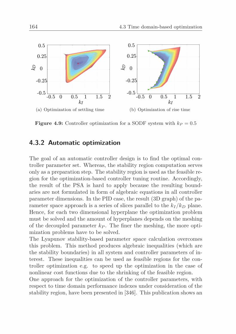
164 4.3 Time domain-based optimization
(a) Optimization of settling time (b) Optimization of rise time
Figure 4.9: Controller optimization for a SODF system with kP = 0.5
4.3.2 Automatic optimization
The goal of an automatic controller design is to find the optimal con-troller parameter set. Whereas, the stability region computation servesonly as a preparation step. The stability region is used as the feasible re-gion for the optimization-based controller tuning routine. Accordingly,the result of the PSA is hard to apply because the resulting bound-aries are not formulated in form of algebraic equations in all controllerparameter dimensions. In the PID case, the result (3D graph) of the pa-rameter space approach is a series of slices parallel to the kI/kD plane.Hence, for each two dimensional hyperplane the optimization problemmust be solved and the amount of hyperplanes depends on the meshingof the decoupled parameter kP . The finer the meshing, the more opti-mization problems have to be solved.The Lyapunov stability-based parameter space calculation overcomesthis problem. This method produces algebraic inequalities (which arethe stability boundaries) in all system and controller parameters of in-terest. These inequalities can be used as feasible regions for the con-troller optimization e.g. to speed up the optimization in the case ofnonlinear cost functions due to the shrinking of the feasible region.One approach for the optimization of the controller parameters, withrespect to time domain performance indexes under consideration of thestability region, have been presented in [346]. This publication shows an
4 Performance-based synthesis 165
implementation of the optimization of settling time without overshoot.The problem is solved by using a big bang big crunch optimizationstrategy.In [155] various numerical non-convex optimization techniques for sev-eral time domain performance indexes are illustrated.Next, an analytical controller parameter optimization is presented byusing the H2 norm for delay-free systems11. The H2 norm is chosen asperformance index because the H2 cost function can be formulated inan easy algebraic equation as presented in the following. From the H2norm controller optimization can be obtained a controller parameter setwhich minimizes the maximum impulse disturbance. In general, smallcontroller gains result from this optimization. Therefore, it is often usedto calculate energy efficient controller parameters [45, 193, 298]. For atransparent insight, this optimization method is demonstrated basedon a practical application example in section 5.4. The H2 objectivefunction can be stated as
||G(s)||22 =1
2π
∞∫−∞
tr(G(jω)HG(jω))dω
where �H symbolizes the conjugate transposed value. By using theParseval theorem, this objective function can be rewritten to simplifythe optimization. In continuous time domain, Parseval’s theorem states[220]
12πj
j∞∫−j∞
X1(−s)HX2(s)ds =∞∫
−∞x1(t)ᵀx2(t)dt.
For discrete signals, based on [256] a similar correlation yields
12π
π∫−π
X1(e jω)HX2(e−jω)dω =∞∑
k=−∞x1(k)ᵀx2(k).
11A first implementation and discussion of the proposed ideas have been presentedin [S06, S39, S41]. The following section is based on this. The key ideas of thissection were published during the project AB 65/2-3 in [271]
166 4.3 Time domain-based optimization
Consequently, for strictly proper MIMO systems using the Parseval the-orem and the observability or controllability gramian P O or P C (section2.9), the H2 cost function becomes:
||G(s)||22 = ||g(t)||22 =∞∫
0
tr(g(t)ᵀg(t)
)dt
=∞∫
0
tr(
BᵀeAᵀtCᵀCeAtB)
dt
= tr
⎛⎜⎝Bᵀ∞∫
0
eAᵀtCᵀCeAtdtB
⎞⎟⎠= tr (BᵀP OB) = tr (CP CCᵀ)
||G(z)||22 = ||g(k)||22 =∞∑
k=0tr(g(k)ᵀg(k)
)=
∞∑k=0
tr(
BᵀeAᵀkCᵀCeAkB)
= tr
⎛⎝Bᵀ∞∑
k=0eAᵀkCᵀCeAkB
⎞⎠= tr
(BᵀP O(k))B
)= tr
(CP C(k)Cᵀ)
where g(t) and g(k) are the impulse responses.The benefit in the explicit consideration of the stability boundaries isobvious in the case of the H2 optimization because the presented H2 costfunction is only defined for stable controller parameter combinations. Inprinciple, the idea of using the H2 cost function for the controller tun-ing under explicit consideration of the Lyapunov stability boundaries issimilar to the classical H∞ frameworks (see [194]) which are discussedin the next section.In the same way like the H2 optimization, an alternative objective func-tion can be stated by using the integral square error (ISE) [220]. Itquantifies the deviation of the step response of the system from an ideal
4 Performance-based synthesis 167
step response. Consequently, the objective function
J =∞∫
−∞e(t)2dt =
∞∫−∞
(y(t)− 1)2dt
results. This can be rewritten by using Parseval’s theorem
J =1
2π
∞∫−∞
E(jω)HE(jω)dω
with E(jω) = G(jω) 1jω −
1jω . For an intuitive insight to the ISE opti-
mization, consider a first order system in the form
G(jω) =1
1 + T jω
with the free adjustable time constant T . For this system the ISE costfunction results to
J =1
2π
∞∫−∞
E(jω)HE(jω)dω =1
2π
∞∫−∞
−T
T jω + 1−T
T jω + 1dω
=1
2π
∞∫−∞
T 2
T 2ω2 + 1dω =
12π
[T atan(Tx)
]∞
−∞=
T
2.
Accordingly, it is easy to see how the time constant influences the ISEin this example. As expected, the ISE becomes minimal for a minimalvalue of T . The value set of T can be constrained by using the stabilityand performance boundaries of the system, which could be calculatedas discussed in sections 2 and 4.1.The same procedure can be applied similarly for more advanced prob-lems. In such cases, the cost functions become more advanced and willbe in most cases nonlinear. In section 5.6., there is a practical applica-tion example presented which uses the H2 and ISE optimization for thecontroller tuning.
168 4.3 Time domain-based optimization
In the following, a brief introduction of strategies to solve constrainednonlinear optimization problems, introduced previously, is provided.Different solution strategies for constrained nonlinear optimization prob-lems are discussed e.g. in [42,66,224,242]. In the following, an interior-point method is used to solve the minimization problem, similar to[66, 224, 242]. The optimization problem consists of equality c(k) = 0and j inequality boundary conditions h(k) − s = 0 with s ≥ 0. Theinequality boundary conditions are transformed into equality boundaryconditions by using the slag variable s and a logarithmic penalty func-tion. The problem can be formulated by using Lagrange multipliers:
L(k,s,λ) = f(k)−Ψj∑
i=1ln si − λᵀ
hh(k)− λᵀc (c(k) + s)
with the multipliers λh and λc. Through the application of the necessaryoptimality conditions defined by the Kuhn-Tucker condition it results
∇kL(k,s,λ) = ∇f(k)− Jh(k)ᵀλh − Jc(k)ᵀλc = 0Sλc −Ψe = 0
h(k) = 0c(k)− s = 0
with e = [1,...,1]ᵀ, S = diag(s) and the Jacobi matrices Jh and Jc.This optimization problem can be solved by standard methods like linesearch or trust region methods. In this dissertation, the fmincon ofMatlab has been employed to solve the problem. The algorithm switchesfrom an easy line search to a more complex trust region sequentialquadratic programming (SQP) method if the Hessian matrix ∇2
kkL isnot positive definite or the slag variable s or the multiplier λc are nearlyzero [224]. Quadratic problems are iteratively solved at each iterationstep kk instead of solving the complex nonlinear problem directly. Inthe case of an SQP, this leads to
mindk,ds
∇f(kk)ᵀdk +12
dᵀk∇2
kkL(k,s,λ)dk − μeᵀS−1ds +12
dᵀs S−1Λds
with Jh(kk)ᵀdk + h(kkk) = 0Jh(kk)ᵀdk + ds + g(kk) + sk = 0dk,ds ∈ Tk
with the search direction d and the trust region TK . A SQP optimiza-tion algorithm have been presented in [66] in detail.
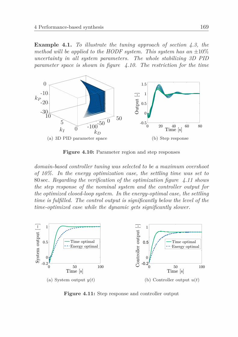
4 Performance-based synthesis 169
Example 4.1. To illustrate the tuning approach of section 4.3, themethod will be applied to the HODF system. This system has an ±10%uncertainty in all system parameters. The whole stabilizing 3D PIDparameter space is shown in figure 4.10. The restriction for the time
-100-50 0 50
05
10-30-20-100
kP
kDkI
(a) 3D PID parameter space (b) Step response
Figure 4.10: Parameter region and step responses
domain-based controller tuning was selected to be a maximum overshootof 10%. In the energy optimization case, the settling time was set to80 sec. Regarding the verification of the optimization figure 4.11 showsthe step response of the nominal system and the controller output forthe optimized closed-loop system. In the energy-optimal case, the settlingtime is fulfilled. The control output is significantly below the level of thetime-optimized case while the dynamic gets significantly slower.
(a) System output y(t) (b) Controller output u(t)
Figure 4.11: Step response and controller output
170 4.4 Frequency domain-based optimization
Remark: A variety of LMI-based optimization tools is available today,see e.g. [141, 318]. These tools follow a similar idea like the proposedcontroller optimization approaches in this dissertation. They use pow-erful numerical tools to search for the best fitting controller gains basedon LMIs which are based on e.g. the Lyapunov equation. The alreadypresented methods are less conservative and more flexible (they canhandle different system types) as well as more transparent due to theanalytical basis of the calculation. Therefore, they offer a better under-standing of the underling methods as well as a tool for the verificationof the results. However, the polynomial optimization methods are com-putationally more efficient in comparison to all the mentioned methods.But, the computational cost grows strongly with increasing system di-mension and complexity of the cost-function. The computational effortincreases also dramatically in the case of non-convex stability regionsdue to the need of convex approximations for such regions.
4.4 Frequency domain-based optimizationIn some cases it is not sufficient to consider only time domain tuninggoals. Accordingly, the use of frequency domain-based performanceindexes can help.
4.4.1 Performance mapsSome frequency domain-based performance mapping techniques are pre-sented in the following to guide the user during the controller tuningthrough the stability regions.
Gain, phase and delay margin12 The gain margin AM and the phasemargin ϕM are classical stability criteria. These margins offer informa-tion how much the gain and phase of a system can be increased beforethe closed-loop system becomes unstable. The margins are defined as:
AM =1
|G(jωπ)ϕM = π + ∠G(jωc) (4.3)
This classical definition is visualized in figure 4.13. The gain margin isnormally chosen in a range between 1.5 (good disturbance rejection) up12A first implementation and discussion of the proposed ideas have been presented
in [S19, S40]. The following section is based on this.
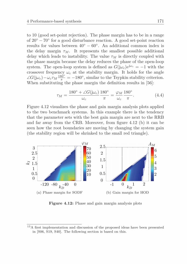
4 Performance-based synthesis 171
to 10 (good set-point rejection). The phase margin has to be in a rangeof 20◦− 70◦ for a good disturbance reaction. A good set-point reactionresults for values between 40◦ − 60◦. An additional common index isthe delay margin τM . It represents the smallest possible additionaldelay which leads to instability. The value τM is directly coupled withthe phase margin because the delay reduces the phase of the open-loopsystem. The open-loop system is defined as G(jωc)ejωc = −1 with thecrossover frequency ωc at the stability margin. It holds for the angle∠G(jωc)−ωcτM
180◦π = −180◦, similar to the Tsypkin stability criterion.
When substituting the phase margin the definition results in [56]:
τM =180◦ + ∠G(jωc)
ωc
180◦
π=
ϕM
ωc
180◦
π. (4.4)
Figure 4.12 visualizes the phase and gain margin analysis plots appliedto the two benchmark systems. In this example there is the tendencythat the parameter sets with the best gain margin are next to the RRBand far away from the CRB. Moreover, from figure 4.12 (b) it can beseen how the root boundaries are moving by changing the system gain(the stability region will be shrinked to the small red triangle).
32.521.510.50
-120 -80 -40 0
10203040506070
ϕM
kI
kD
(a) Phase margin for SODF
2.521.51
0.50
-1 0 1 2
23456
AM
kD
(b) Gain margin for HOD
Figure 4.12: Phase and gain margin analysis plots
13A first implementation and discussion of the proposed ideas have been presentedin [S06, S19, S40]. The following section is based on this.
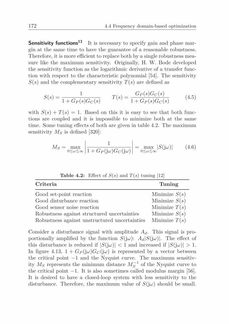
172 4.4 Frequency domain-based optimization
Sensitivity functions13 It is necessary to specify gain and phase mar-gin at the same time to have the guarantee of a reasonable robustness.Therefore, it is more efficient to replace both by a single robustness mea-sure like the maximum sensitivity. Originally, H. W. Bode developedthe sensitivity function as the logarithmic derivative of a transfer func-tion with respect to the characteristic polynomial [54]. The sensitivityS(s) and the complementary sensitivity T (s) are defined as
S(s) =1
1 + GP (s)GC(s)T (s) =
GP (s)GC(s)1 + GP (s)GC(s)
(4.5)
with S(s) + T (s) = 1. Based on this it is easy to see that both func-tions are coupled and it is impossible to minimize both at the sametime. Some tuning effects of both are given in table 4.2. The maximumsensitivity MS is defined [320]:
MS = max0≤ω≤∞
∣∣∣∣ 11 + GP (jω)GC(jω)
∣∣∣∣ = max0≤ω≤∞
|S(jω)| (4.6)
Table 4.2: Effect of S(s) and T (s) tuning [12]
Criteria Tuning
Good set-point reaction Minimize S(s)Good disturbance reaction Minimize S(s)Good sensor noise reaction Minimize T (s)Robustness against structured uncertainties Minimize S(s)Robustness against unstructured uncertainties Minimize T (s)
Consider a disturbance signal with amplitude Ad. This signal is pro-portionally amplified by the function S(jω): Ad|S(jω)|. The effect ofthis disturbance is reduced if |S(jω)| < 1 and increased if |S(jω)| > 1.In figure 4.13, 1 + GP (jω)GC(jω) is represented by a vector betweenthe critical point −1 and the Nyquist curve. The maximum sensitiv-ity MS represents the minimum distance M−1
S of the Nyquist curve tothe critical point −1. It is also sometimes called modulus margin [56].It is desired to have a closed-loop system with less sensitivity to thedisturbance. Therefore, the maximum value of S(jω) should be small.
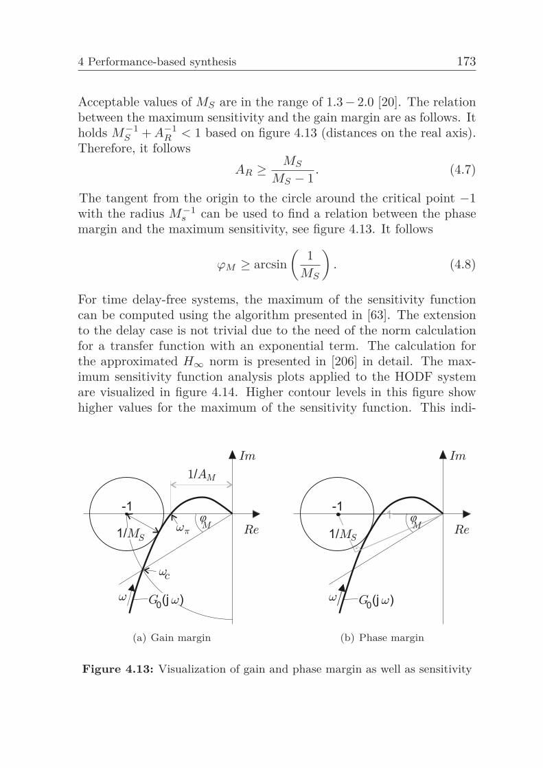
4 Performance-based synthesis 173
Acceptable values of MS are in the range of 1.3− 2.0 [20]. The relationbetween the maximum sensitivity and the gain margin are as follows. Itholds M−1
S + A−1R < 1 based on figure 4.13 (distances on the real axis).
Therefore, it followsAR ≥
MS
MS − 1. (4.7)
The tangent from the origin to the circle around the critical point −1with the radius M−1
s can be used to find a relation between the phasemargin and the maximum sensitivity, see figure 4.13. It follows
ϕM ≥ arcsin(
1MS
). (4.8)
For time delay-free systems, the maximum of the sensitivity functioncan be computed using the algorithm presented in [63]. The extensionto the delay case is not trivial due to the need of the norm calculationfor a transfer function with an exponential term. The calculation forthe approximated H∞ norm is presented in [206] in detail. The max-imum sensitivity function analysis plots applied to the HODF systemare visualized in figure 4.14. Higher contour levels in this figure showhigher values for the maximum of the sensitivity function. This indi-
(a) Gain margin (b) Phase margin
Figure 4.13: Visualization of gain and phase margin as well as sensitivity
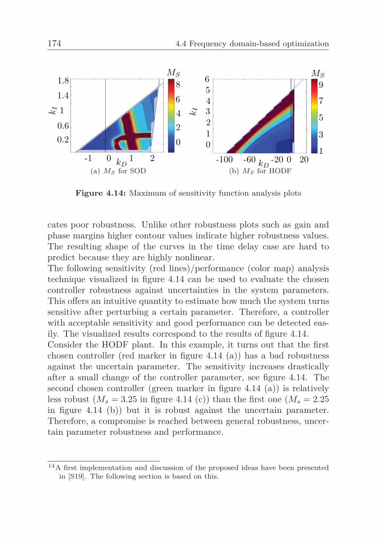
174 4.4 Frequency domain-based optimization
1.81.41
0.60.2
-1 0 1 2
02468
MS
kI
kD(a) MS for SOD
6543210
-100 -60 -20 0 201
3
5
7
9MS
kI
kD(b) MS for HODF
Figure 4.14: Maximum of sensitivity function analysis plots
cates poor robustness. Unlike other robustness plots such as gain andphase margins higher contour values indicate higher robustness values.The resulting shape of the curves in the time delay case are hard topredict because they are highly nonlinear.The following sensitivity (red lines)/performance (color map) analysistechnique visualized in figure 4.14 can be used to evaluate the chosencontroller robustness against uncertainties in the system parameters.This offers an intuitive quantity to estimate how much the system turnssensitive after perturbing a certain parameter. Therefore, a controllerwith acceptable sensitivity and good performance can be detected eas-ily. The visualized results correspond to the results of figure 4.14.Consider the HODF plant. In this example, it turns out that the firstchosen controller (red marker in figure 4.14 (a)) has a bad robustnessagainst the uncertain parameter. The sensitivity increases drasticallyafter a small change of the controller parameter, see figure 4.14. Thesecond chosen controller (green marker in figure 4.14 (a)) is relativelyless robust (Ms = 3.25 in figure 4.14 (c)) than the first one (Ms = 2.25in figure 4.14 (b)) but it is robust against the uncertain parameter.Therefore, a compromise is reached between general robustness, uncer-tain parameter robustness and performance.
14A first implementation and discussion of the proposed ideas have been presentedin [S19]. The following section is based on this.
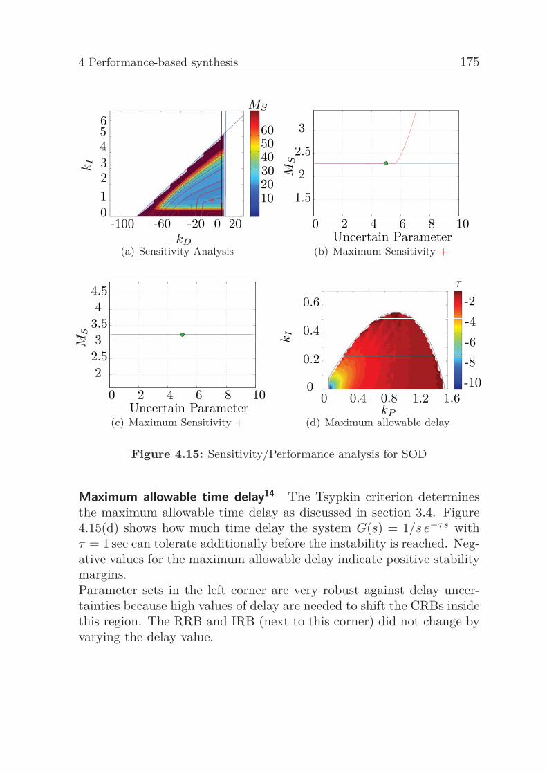
4 Performance-based synthesis 175
6543210
-100 -60 -20 0 20
605040302010
MS
kI
kD(a) Sensitivity Analysis
0 2 4 6 8 10
1.5
2
2.5
3
Uncertain Parameter
MS
(b) Maximum Sensitivity +
0 2 4 6 8 10
22.53
3.54
4.5
Uncertain Parameter
MS
(c) Maximum Sensitivity +
0.6
0.4
0.2
00 0.4 0.8 1.2 1.6
-2-4-6-8-10
τ
kP
kI
(d) Maximum allowable delay
Figure 4.15: Sensitivity/Performance analysis for SOD
Maximum allowable time delay14 The Tsypkin criterion determinesthe maximum allowable time delay as discussed in section 3.4. Figure4.15(d) shows how much time delay the system G(s) = 1/s e−τs withτ = 1 sec can tolerate additionally before the instability is reached. Neg-ative values for the maximum allowable delay indicate positive stabilitymargins.Parameter sets in the left corner are very robust against delay uncer-tainties because high values of delay are needed to shift the CRBs insidethis region. The RRB and IRB (next to this corner) did not change byvarying the delay value.
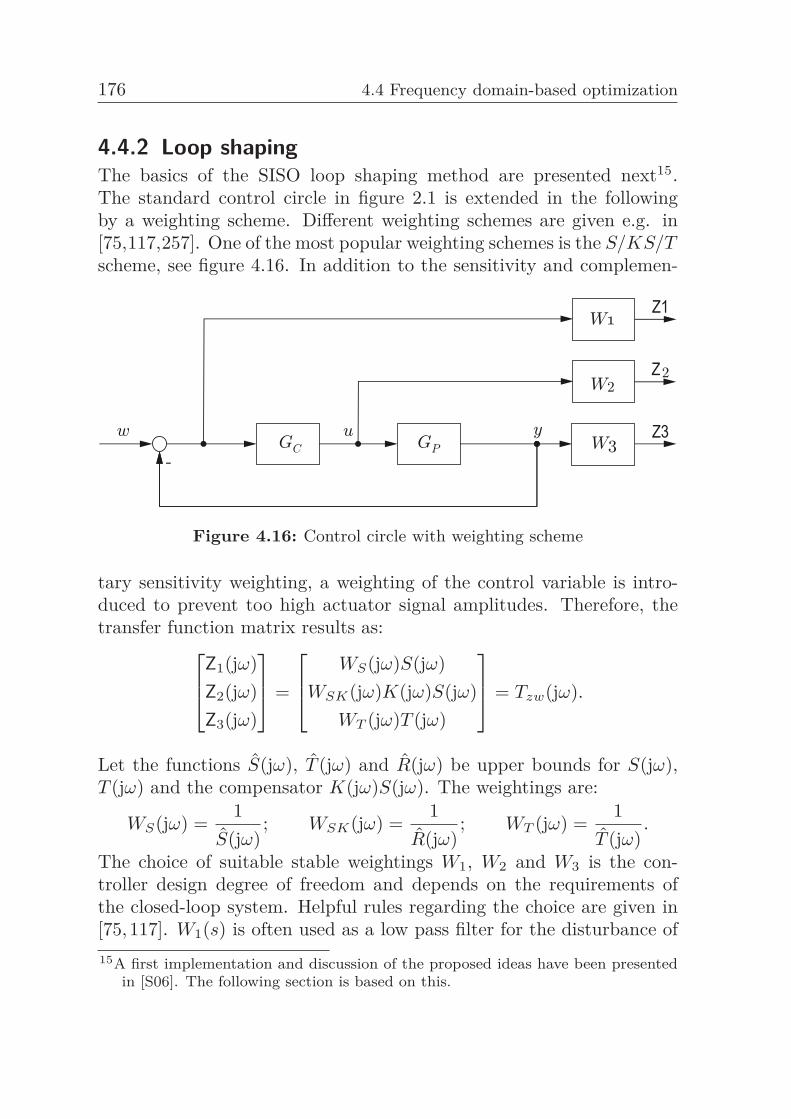
176 4.4 Frequency domain-based optimization
4.4.2 Loop shapingThe basics of the SISO loop shaping method are presented next15.The standard control circle in figure 2.1 is extended in the followingby a weighting scheme. Different weighting schemes are given e.g. in[75,117,257]. One of the most popular weighting schemes is the S/KS/Tscheme, see figure 4.16. In addition to the sensitivity and complemen-
Figure 4.16: Control circle with weighting scheme
tary sensitivity weighting, a weighting of the control variable is intro-duced to prevent too high actuator signal amplitudes. Therefore, thetransfer function matrix results as:⎡⎢⎣Z1(jω)
Z2(jω)Z3(jω)
⎤⎥⎦ =
⎡⎢⎣ WS(jω)S(jω)WSK(jω)K(jω)S(jω)
WT (jω)T (jω)
⎤⎥⎦ = Tzw(jω).
Let the functions S(jω), T (jω) and R(jω) be upper bounds for S(jω),T (jω) and the compensator K(jω)S(jω). The weightings are:
WS(jω) =1
S(jω); WSK(jω) =
1R(jω)
; WT (jω) =1
T (jω).
The choice of suitable stable weightings W1, W2 and W3 is the con-troller design degree of freedom and depends on the requirements ofthe closed-loop system. Helpful rules regarding the choice are given in[75, 117]. W1(s) is often used as a low pass filter for the disturbance of15A first implementation and discussion of the proposed ideas have been presented
in [S06]. The following section is based on this.
4 Performance-based synthesis 177
frequencies below the bandwidth to reduce the sensitivity S(s) in thisrange, see figure 4.19. The limitation of S(s) for higher frequencies al-lows the specification of a minimum phase margin in order to increasethe robustness against phase shifting model uncertainties. W2(s) isoften parametrized as a high pass filter to reduce the complementarysensitivity T (s) for high frequencies [75].A standard tool for controller tuning which uses the previously intro-duced weighting matrices is the H∞ synthesis. For details about H∞,see e.g [75,208,257,352]. The design requirements are set up through fre-quency response shaping. In the single-loop case, this is done by shapingthe amplitude response and in the multi-variable case by shaping the sin-gular value curves [118]. The H∞ norm of a transfer function G(s) rep-resents the maximum absolute value of G(s). The goal of the H∞ con-troller synthesis is to minimize the H∞ norm Tzω(s). Therefore, the H∞problem is stated as [208]:‖ G ‖∞= supω | G(jω) |⇒ min
∥∥Tzω(s)∥∥
∞.A first solution of the H∞ problem was presented by B. A. Francis in1987 [106] which resulted in high dimensional controller orders. J. C.Doyle et al. [92] presented a Riccati equation-based iterative method tominimize ||Tzw||∞ < γ in 1988. P. Gahinet and P. Apkarian modifiedthis approach into a LMI-based method [111]. In general, it is difficultto specify the controller structure which should result after the H∞optimization. Usually, a controller with the same order as the plantresults. Afterwards, model reduction methods can be used to reducethe controller order. An H∞-based PID controller tuning have beenpresented in [15].However, one of the biggest remaining challenges is to deal with timedelays in this method. Different methods to solve this problem arediscussed in [104, 257]. There, they conclude that the Padé delay ap-proximation is the most suitable way to overcome the problem of solvingthe infinite dimensional Riccati equation. Other approaches are limitedto very restricted conditions for the plant [1]. M. S. Mahmoud pre-sented in [194] a formulation which is based on a Lyapunov stability-based mapping of the delay system of the optimization problem in formof finite dimensional Riccati equations which can be solved effectivelythrough LMI software tools. Due to the conservatism of the Lyapunovstability-based mapping its results become conservative. An efficientapproximation-based H∞ optimization strategy for delay systems isshown in [206].
178 4.4 Frequency domain-based optimization
Least squares loop shaping - numerically16 A numerical least squareloop shaping approach for PID controllers which use the stabilizing con-troller parameter region will be shown in the following.This approach is applicable for delay systems without delay approx-imation. Similar to the H∞ method, suitable weightings have to bechosen:
|S(jω,kP ,kI ,kD)| ≤ |WS(ω)−1||T (jω,kP ,kI ,kD)| ≤ |WT (ω)−1| (4.9)|KS(jω,kP ,kI ,kD)| ≤ |WKS(ω)−1|
The resulting optimization problem can be stated in the form
f(k) =r∑
i=1(|S(jωi,k)| − |WS(jωi)|)2 +
r∑i=1
(|T (jωi,k)| − |WT (jωi)|)2+
r∑i=1
(|KS(jωi,k)| − |WKS(jωi)|)2
with m sampling points. The least squares method is a standard toolfor the calculation of the constant parameter k of a function f(t) byusing r measurement pairs (t1,...,tr, y1,...,yr). To reduce the effect ofmeasurement errors, it should hold: r � n. The goal of the leastsquares optimization is to find a function f(t) which matches best withthe desired values y. The difference ri = g(ti,k)−yi with i = 1, 2,..., ris named residual. For more information see [50,107,278].Due to the nonlinear dependency of the optimization parameters k andg(t) a nonlinear least squares (NLLSQ) approach is needed to realizea least squares loop shaping. Such problems can be solved throughmethods which are presented in [50, 83, 107]. The easiest method tosolve a NLLSQ problem is to use the Gauss-Newton-method. Therefore,the problem is reformulated as mink∈Rn f(k), f(k) = 0.5‖r(k)‖2
2 =0.5
∑mi=1 r2
i (k), m ≥ n.. The conditions for a local minimum are given
16A first implementation and discussion of the proposed ideas have been presentedin [S06]. The following section is based on this. The key ideas of this sectionwere published during the project AB 65/2-3 in [271].
4 Performance-based synthesis 179
by:
∇f(k∗) = Jr(k∗)ᵀr(k∗) = 0 (4.10a)
∇2f(k∗) = Jr(k∗)ᵀJr(k∗) +m∑
i=1ri(k)∇2ri(k) > 0 (4.10b)
with the Jacobi matrix Jr(k) of the residual vector r in the form:
Jr(k) =
⎡⎢⎢⎢⎢⎣∂r1(k)
∂k1· · · ∂r1(k)
∂kn
......
∂rr(k)∂k1
· · · ∂rr(k)∂kn
⎤⎥⎥⎥⎥⎦ (4.11)
The resulting system of n nonlinear equations cannot be solved analyt-ically in general. A numerical solution of equation (4.10a) is computa-tional expensive. Therefore, the residual equations need to be linearizede.g. by using the Newton method. The iterative relation results in:
sk =∇f(kk)∇2f(kk)
kk+1 = kk − sk. By using equation (4.10) results:
[Jr(kk)ᵀJr(kk +r∑
i=1ri(kk∇2ri(kk)]sk = Jr(kk)ᵀr(kk). (4.12)
The right hand side of equation (4.10b) is neglected (‖f(k∗)‖ 1) toreduce the computational complexity. Therefore it follows:
Jr(kk)ᵀJr(kk)sk = Jr(kk)ᵀr(kk) (4.13a)kk+1 = kk − sk. (4.13b)
In each iteration the following linear least squares problem has to besolved based on equation (4.13a):
mins∈Rn
‖r(kk) + J(kk)s‖2 (4.14)
Constraints have to be added to the optimization problem to restrictthe solver to the stabilizing parameter region and to prevent a violation
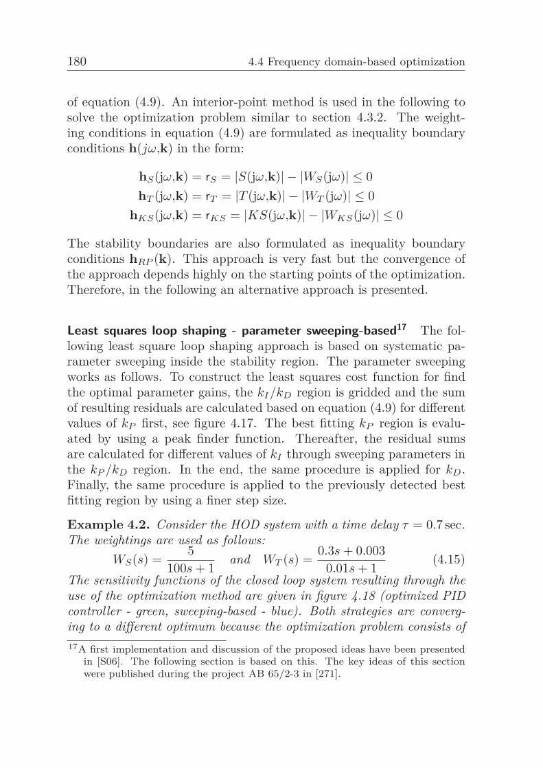
180 4.4 Frequency domain-based optimization
of equation (4.9). An interior-point method is used in the following tosolve the optimization problem similar to section 4.3.2. The weight-ing conditions in equation (4.9) are formulated as inequality boundaryconditions h(jω,k) in the form:
hS(jω,k) = rS = |S(jω,k)| − |WS(jω)| ≤ 0hT (jω,k) = rT = |T (jω,k)| − |WT (jω)| ≤ 0
hKS(jω,k) = rKS = |KS(jω,k)| − |WKS(jω)| ≤ 0
The stability boundaries are also formulated as inequality boundaryconditions hRP (k). This approach is very fast but the convergence ofthe approach depends highly on the starting points of the optimization.Therefore, in the following an alternative approach is presented.
Least squares loop shaping - parameter sweeping-based17 The fol-lowing least square loop shaping approach is based on systematic pa-rameter sweeping inside the stability region. The parameter sweepingworks as follows. To construct the least squares cost function for findthe optimal parameter gains, the kI/kD region is gridded and the sumof resulting residuals are calculated based on equation (4.9) for differentvalues of kP first, see figure 4.17. The best fitting kP region is evalu-ated by using a peak finder function. Thereafter, the residual sumsare calculated for different values of kI through sweeping parameters inthe kP /kD region. In the end, the same procedure is applied for kD.Finally, the same procedure is applied to the previously detected bestfitting region by using a finer step size.
Example 4.2. Consider the HOD system with a time delay τ = 0.7 sec.The weightings are used as follows:
WS(s) =5
100s + 1and WT (s) =
0.3s + 0.0030.01s + 1
(4.15)The sensitivity functions of the closed loop system resulting through theuse of the optimization method are given in figure 4.18 (optimized PIDcontroller - green, sweeping-based - blue). Both strategies are converg-ing to a different optimum because the optimization problem consists of17A first implementation and discussion of the proposed ideas have been presented
in [S06]. The following section is based on this. The key ideas of this sectionwere published during the project AB 65/2-3 in [271].
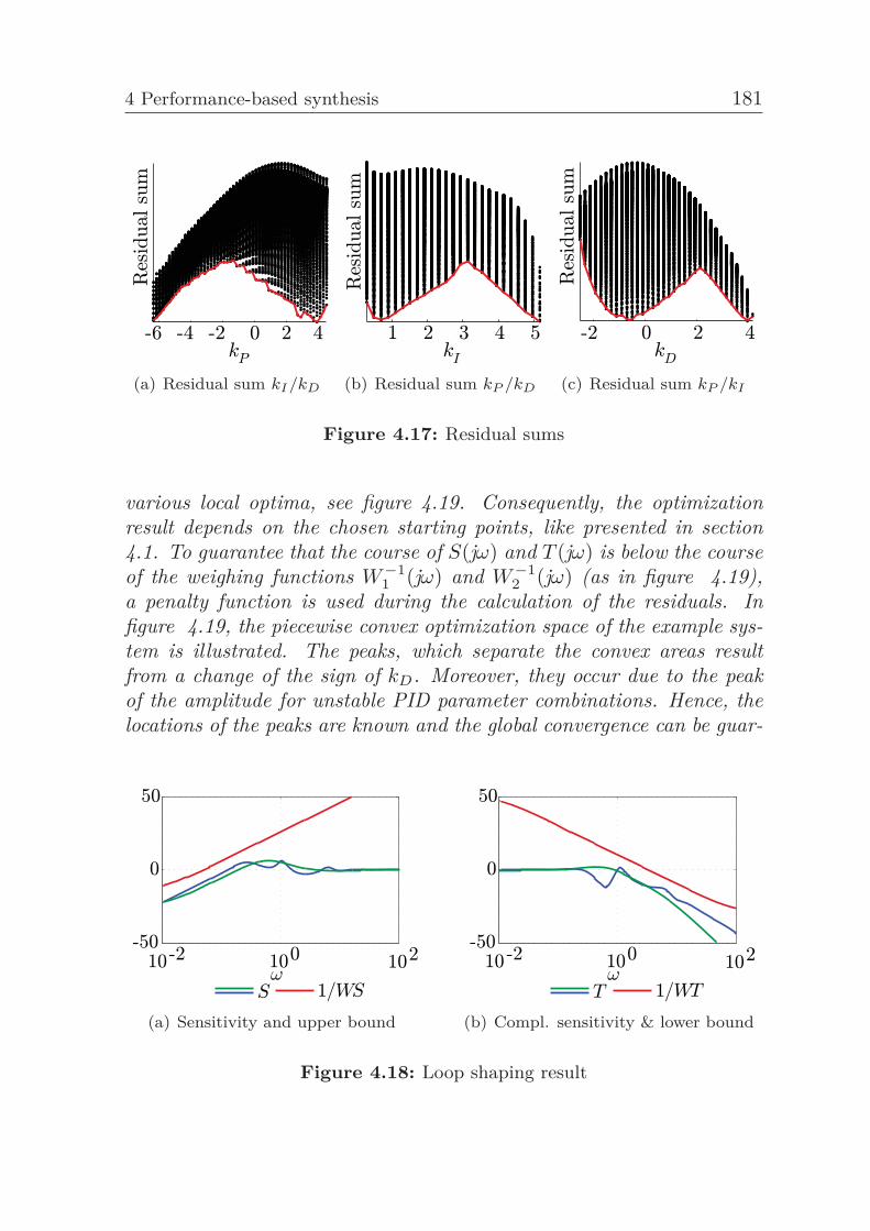
4 Performance-based synthesis 181
(a) Residual sum kI/kD (b) Residual sum kP /kD (c) Residual sum kP /kI
Figure 4.17: Residual sums
various local optima, see figure 4.19. Consequently, the optimizationresult depends on the chosen starting points, like presented in section4.1. To guarantee that the course of S(jω) and T (jω) is below the courseof the weighing functions W −1
1 (jω) and W −12 (jω) (as in figure 4.19),
a penalty function is used during the calculation of the residuals. Infigure 4.19, the piecewise convex optimization space of the example sys-tem is illustrated. The peaks, which separate the convex areas resultfrom a change of the sign of kD. Moreover, they occur due to the peakof the amplitude for unstable PID parameter combinations. Hence, thelocations of the peaks are known and the global convergence can be guar-
(a) Sensitivity and upper bound (b) Compl. sensitivity & lower bound
Figure 4.18: Loop shaping result
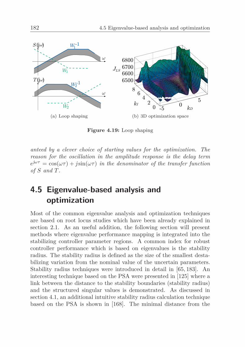
182 4.5 Eigenvalue-based analysis and optimization
(a) Loop shaping (b) 3D optimization space
Figure 4.19: Loop shaping
anteed by a clever choice of starting values for the optimization. Thereason for the oscillation in the amplitude response is the delay termejωτ = cos(ωτ) + j sin(ωτ) in the denominator of the transfer functionof S and T .
4.5 Eigenvalue-based analysis andoptimization
Most of the common eigenvalue analysis and optimization techniquesare based on root locus studies which have been already explained insection 2.1. As an useful addition, the following section will presentmethods where eigenvalue performance mapping is integrated into thestabilizing controller parameter regions. A common index for robustcontroller performance which is based on eigenvalues is the stabilityradius. The stability radius is defined as the size of the smallest desta-bilizing variation from the nominal value of the uncertain parameters.Stability radius techniques were introduced in detail in [65, 183]. Aninteresting technique based on the PSA were presented in [125] where alink between the distance to the stability boundaries (stability radius)and the structured singular values is demonstrated. As discussed insection 4.1, an additional intuitive stability radius calculation techniquebased on the PSA is shown in [168]. The minimal distance from the
4 Performance-based synthesis 183
stability boundaries is denoted as the radius of the largest hyperspherein the Q space. Accordingly, the minimum distance from the RRB, theCRB and the IRB are obtained. Unfortunately, this technique doesn’tconsider the effect of parameter uncertainties onto the eigenvalue lo-cation directly, as presented next. To overcome this drawback, somealternative approaches are presented in the following.
Stability radius and pseudospectra18 An interesting way to computethe stability radius is via ε-pseudospectra techniques [206, 334]. Thesensitivity of eigenvalues regarding parameter changes can be explainedthrough the comparison of the eigenvalues of the nominal system withthe eigenvalues of the perturbed system. The set of eigenvalues of theperturbed system is called ε-pseudospectrum. The magnitude of un-structured uncertainties ε is calculated by using the Frobenius normor 2-norm where ||A||F |2 < ε holds. For a matrix A with dimensionm×n, the Frobenius norm is defined as ||A||F =
√∑mi=1
∑nj=1 |aij |2 =√∑min(m,n)
i=1 σ2i where σi are the singular values of A. After apply-
ing the perturbation E, the resulting set of eigenvalues can be foundby solving the eigenvalue equation (A + E)v = sv with the normalizedeigenvectors |v| = 1 where s are the perturbed eigenvalues. The parame-ter perturbation matrix is defined as E = s u v∗ where s < ε and |u| = 1holds. Therefore, the resolvent of the matrix A is R(s) = (A − sI)−1.Rewriting the equation of the perturbed eigenvalues in terms of theresolvent and perturbation leads to:
(A + E)v = s v ⇒ s v −A v = E v ⇒ −(A− s I)v = s u v∗v
⇒ −s−1(A− s I)−1(A− s I)v = s−1(A− s I)−1s u
⇒ −s−1v = (A− s I)−1u⇒ −s−1v = R(s)u
This gives ||R(s)u|| = || − s−1v|| ⇒ ||R(s)|| ||u|| ≥ ||R(s)u|| = −s−1||v||⇒ ||R(s)|| ≥ s−1 > ε−1. Consequently, the ε-pseudospectrum is definedas αε = ||R(s)||−1 < ε. The largest singular value of a matrix is equal tothe matrix Frobenius norm. Additionally, the largest singular value ofthe matrix’s inverse is equal to the inverse of the smallest singular value.18A first implementation and discussion of the proposed ideas have been presented
in [S19]. The following section is based on this.
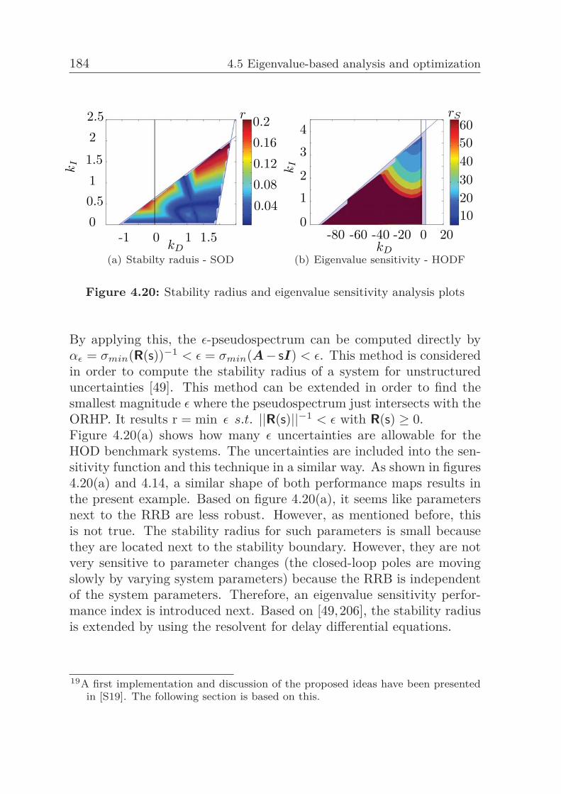
184 4.5 Eigenvalue-based analysis and optimization
2.52
1.510.50
-1 0 1 1.5
0.040.080.120.160.2r
kI
kD
(a) Stabilty raduis - SOD
4
3
2
1
0-80 -60 -40 -20 0 20
102030405060
rS
kI
kD(b) Eigenvalue sensitivity - HODF
Figure 4.20: Stability radius and eigenvalue sensitivity analysis plots
By applying this, the ε-pseudospectrum can be computed directly byαε = σmin(R(s))−1 < ε = σmin(A− sI) < ε. This method is consideredin order to compute the stability radius of a system for unstructureduncertainties [49]. This method can be extended in order to find thesmallest magnitude ε where the pseudospectrum just intersects with theORHP. It results r = min ε s.t. ||R(s)||−1 < ε with R(s) ≥ 0.Figure 4.20(a) shows how many ε uncertainties are allowable for theHOD benchmark systems. The uncertainties are included into the sen-sitivity function and this technique in a similar way. As shown in figures4.20(a) and 4.14, a similar shape of both performance maps results inthe present example. Based on figure 4.20(a), it seems like parametersnext to the RRB are less robust. However, as mentioned before, thisis not true. The stability radius for such parameters is small becausethey are located next to the stability boundary. However, they are notvery sensitive to parameter changes (the closed-loop poles are movingslowly by varying system parameters) because the RRB is independentof the system parameters. Therefore, an eigenvalue sensitivity perfor-mance index is introduced next. Based on [49,206], the stability radiusis extended by using the resolvent for delay differential equations.
19A first implementation and discussion of the proposed ideas have been presentedin [S19]. The following section is based on this.
4 Performance-based synthesis 185
Eigenvalue differential sensitivity19 The distance of the eigenvalues ofthe closed-loop system to the stability boundary is not generally a suf-ficient measurement for robustness because the sensitivity of the eigen-values with respect to parameter variations may be very large. Thissensitivity can be evaluated using the eigenvalue differential sensitivitymethod, based on [334]. This technique can also be considered as a per-formance robustness analysis technique. The eigenvalues of an outputfeedback system Ak = A + B k C are denoted by ev[Ak]. Therefore,the sensitivity of closed-loop eigenvalues with respect to a feedback ma-trix k is ∂evi[Ak]/∂k. The eigenvalues and eigenvectors of the matrixA are calculated by A x = evx where evi are the eigenvalues and vi
are the eigenvectors. Similarly, it holds Ak f�i = f�
i evi[Ak]. By takingthe derivative of both sides using the matrix product rule as well as theKronecker commutative rule between matrix-vector product, the sensi-tivity of an eigenvalue evi[Ak] with respect to k with dimensions m×ncan be expressed by:
∂evi[Ak]∂K
= (Im ⊗ fi�∗T )
∂Ak
∂K(In ⊗ f�
i ) (4.16)
where ⊗ is the Kronecker product, f�i are the right eigenvectors of Ak,
fi� are the left eigenvectors of Ak and Ia is the identity matrix of
dimension a × a. As pointed out before, the sensitivity of the closed-loop pole locations to parameter uncertainties is very high next to theCRB and low next to the RRB. A method which considers the stabilityradius as well as the eigenvalue sensitivity is presented next.
Example 4.3. The previously introduced calculation scheme is shortlypresented in the following example of [334]. Consider the matrices
Ak =(
0 α2 β
), K =
(β α
), m = 1, n = 2.
Assume nominal values of α=-1, and β=-2. This gives:
∂ev1[Ak]∂K
=(
−0.5j0.25 + 0.25j
)ᵀ(0 0 0 10 1 0 0
)(I2 ⊗
(1 + j
2
))
186 4.5 Eigenvalue-based analysis and optimization
=(−0.5j 0.25 + 0.25j
)(0 0 0 10 1 0 0
)⎛⎜⎜⎝1 + j 0
2 00 1 + j0 2
⎞⎟⎟⎠=(0.5 + 0.5j −j
)⇒ ∂ev1[Ak]
∂β= 0.5 + 0.5j and ∂ev1[Ak]
∂α= −j
Hybrid method20 It would be preferable to merge the informationabout the stability radius and the eigenvalue sensitivity to one robust-ness measurement. Therefore, a method to obtain the stability radiusbased on the eigenvalue differential sensitivity is developed in the fol-lowing.An easy method for the stability radius calculation is to determine thedistance between an eigenvalue and the imaginary axis directly. Thiscan be done by calculating the absolute value of the real part of theeigenvalue. This measurement is called spectral abscissa [334].The calculation of the differential sensitivity of the real part of an eigen-value �{∂λi[Ak]} with respect to ∂k with consideration of the stabilityboundary yields to the following equation:
�{∂λi[Ak]M}∂kM
= X ⇒ ∂kM =�{∂λi[Ak]M}
X⇒ ri =
αi[Ak]X
where M denotes stability boundary, αi is the spectral abscissa and nis the number of eigenvalues. The new stability radius is defined byr = min1<i<n ri.Therefore, the change of parameter values which are allowable untilinstability is reached can be calculated. The stability radius of eacheigenvalue is calculated and the worst case radius is obtained, like pre-sented in the following example.This method is presented by using the HODF plant. The coefficient ofthe second order parameter in the denominator is considered as uncer-tain. Figure 4.20(b) shows how much uncertainty can be tolerated in
20A first implementation and discussion of the proposed ideas have been presentedin [S19]. The following section is based on this.
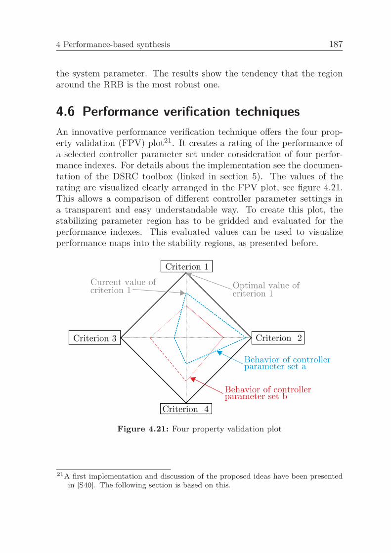
4 Performance-based synthesis 187
the system parameter. The results show the tendency that the regionaround the RRB is the most robust one.
4.6 Performance verification techniquesAn innovative performance verification technique offers the four prop-erty validation (FPV) plot21. It creates a rating of the performance ofa selected controller parameter set under consideration of four perfor-mance indexes. For details about the implementation see the documen-tation of the DSRC toolbox (linked in section 5). The values of therating are visualized clearly arranged in the FPV plot, see figure 4.21.This allows a comparison of different controller parameter settings ina transparent and easy understandable way. To create this plot, thestabilizing parameter region has to be gridded and evaluated for theperformance indexes. This evaluated values can be used to visualizeperformance maps into the stability regions, as presented before.
Figure 4.21: Four property validation plot
21A first implementation and discussion of the proposed ideas have been presentedin [S40]. The following section is based on this.
188
5 Implementation & ApplicationFor the transfer of the developed methods into practical applications theDSRC (Delay System Robust Control) toolbox for Matlab was devel-oped. The first PSA-based toolbox for Matlab was Paradise [156, 214].This toolbox is able to calculate stabilizing controller parameter spacesfor delay-free systems under consideration of restrictions regarding thepole location. A few years later the Robsin toolbox was also developedat the DLR in Oberpfaffenhofen. This toolbox is able to calculate sta-bilizing PID controller parameter spaces for time delay systems [30].Parallel, some similar toolboxes were developed based on the HBT [44].The toolbox PIDrobust which also calculates stabilizing PID controllerparameter spaces for time delay systems was developed at the sametime at the IRT/RWTH in Aachen [146].The DSRC toolbox is the first one which focuses on the stability region-based controller tuning in addition to the stabilizing controller param-eter space calculation. Moreover, the toolbox is not only restricted tosingle-loop PID control structures. Additionally, this toolbox includespowerful tools for the explicit consideration of parameter uncertaintiesin the plant. The intuitive user interface is also a strong selling pointof this toolbox. The toolbox consists of two graphical user interfaces.In the first user interface, the plant structure, the plant parameters aswell as the performance and robustness requirements can be set up. Inthe second user interface, the resulting parameter space can be visual-ized and several controller tuning and analysis tools are given, see figure5.1. The toolbox builds a framework to allow users from different sci-entific disciplines to utilize a simple controller design procedure. Thetoolbox is published under the General Public License and can be down-loaded (http://www.irt.rwth-aachen.de/pidrobust). The web pagecontains a detailed documentation and user manual. Consequently, adetailed presentation of the software is not given in this dissertation.This web page serves also as a central platform for the stability regionresearch. Therefore, the tools from previous projects of the DLR as wellas from the Istanbul University can be accessed on the web page. Thecontact data of currently active research groups in this field can also be
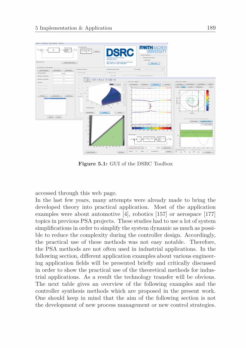
5 Implementation & Application 189
Figure 5.1: GUI of the DSRC Toolbox
accessed through this web page.In the last few years, many attempts were already made to bring thedeveloped theory into practical application. Most of the applicationexamples were about automotive [4], robotics [157] or aerospace [177]topics in previous PSA projects. These studies had to use a lot of systemsimplifications in order to simplify the system dynamic as much as possi-ble to reduce the complexity during the controller design. Accordingly,the practical use of these methods was not easy notable. Therefore,the PSA methods are not often used in industrial applications. In thefollowing section, different application examples about various engineer-ing application fields will be presented briefly and critically discussedin order to show the practical use of the theoretical methods for indus-trial applications. As a result the technology transfer will be obvious.The next table gives an overview of the following examples and thecontroller synthesis methods which are proposed in the present work.One should keep in mind that the aim of the following section is notthe development of new process management or new control strategies.
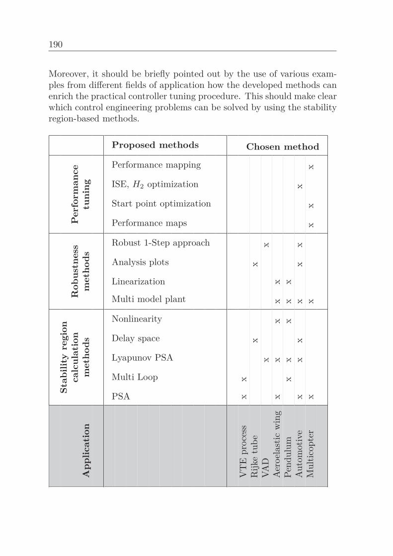
190
Moreover, it should be briefly pointed out by the use of various exam-ples from different fields of application how the developed methods canenrich the practical controller tuning procedure. This should make clearwhich control engineering problems can be solved by using the stabilityregion-based methods.
App
licat
ion
Stab
ility
regi
onca
lcul
atio
nm
etho
dsR
obus
tnes
sm
etho
dsP
erfo
rman
cetu
ning
PSA
Multi Loop
Lyapunov PSA
Delay space
Nonlinearity
Multi model plant
Linearization
Analysis plots
Robust 1-Step approach
Performance maps
Start point optimization
ISE, H2 optimization
Performance mapping
Proposed methods
VT
Epr
oces
sx
x
Chosen method
Rijk
etu
bex
xVA
Dx
xA
eroe
last
icw
ing
xx
xx
xPe
ndul
umx
xx
xx
Aut
omot
ive
xx
xx
xx
xM
ulti
copt
erx
xx
xx
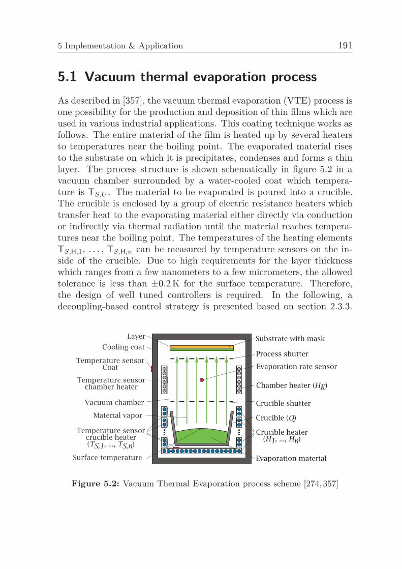
5 Implementation & Application 191
5.1 Vacuum thermal evaporation processAs described in [357], the vacuum thermal evaporation (VTE) process isone possibility for the production and deposition of thin films which areused in various industrial applications. This coating technique works asfollows. The entire material of the film is heated up by several heatersto temperatures near the boiling point. The evaporated material risesto the substrate on which it is precipitates, condenses and forms a thinlayer. The process structure is shown schematically in figure 5.2 in avacuum chamber surrounded by a water-cooled coat which tempera-ture is TS,U . The material to be evaporated is poured into a crucible.The crucible is enclosed by a group of electric resistance heaters whichtransfer heat to the evaporating material either directly via conductionor indirectly via thermal radiation until the material reaches tempera-tures near the boiling point. The temperatures of the heating elementsTS,H,1, . . . , TS,H,n can be measured by temperature sensors on the in-side of the crucible. Due to high requirements for the layer thicknesswhich ranges from a few nanometers to a few micrometers, the allowedtolerance is less than ±0.2 K for the surface temperature. Therefore,the design of well tuned controllers is required. In the following, adecoupling-based control strategy is presented based on section 2.3.3.
Figure 5.2: Vacuum Thermal Evaporation process scheme [274,357]
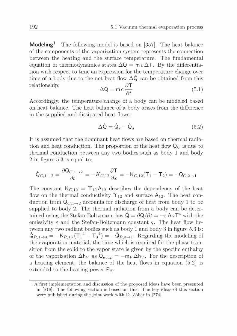
192 5.1 Vacuum thermal evaporation process
Modeling1 The following model is based on [357]. The heat balanceof the components of the vaporization system represents the connectionbetween the heating and the surface temperature. The fundamentalequation of thermodynamics states ΔQ = m c ΔT. By the differentia-tion with respect to time an expression for the temperature change overtime of a body due to the net heat flow ΔQ can be obtained from thisrelationship:
ΔQ = m c∂T∂t
(5.1)
Accordingly, the temperature change of a body can be modeled basedon heat balance. The heat balance of a body arises from the differencein the supplied and dissipated heat flows:
ΔQ = Qs − Qd (5.2)
It is assumed that the dominant heat flows are based on thermal radia-tion and heat conduction. The proportion of the heat flow QC is due tothermal conduction between any two bodies such as body 1 and body2 in figure 5.3 is equal to:
QC,1→2 =∂QC,1→2
∂t= −KC,12
∂T∂x
= −KC,12(T1 − T2) = −QC,2→1
The constant KC,12 = Υ12 A12 describes the dependency of the heatflow on the thermal conductivity Υ12 and surface A12. The heat con-duction term QC,1→2 accounts for discharge of heat from body 1 to besupplied to body 2. The thermal radiation from a body can be deter-mined using the Stefan-Boltzmann law Q = ∂Q/∂t = −ε A ςT4 with theemissivity ε and the Stefan-Boltzmann constant ς. The heat flow be-tween any two radiant bodies such as body 1 and body 3 in figure 5.3 is:QR,1→3 = −KR,13 (T1
4 − T34) = −QR,3→1. Regarding the modeling of
the evaporation material, the time which is required for the phase tran-sition from the solid to the vapor state is given by the specific enthalpyof the vaporization ΔhV as Qevap = −mV ΔhV . For the description ofa heating element, the balance of the heat flows in equation (5.2) isextended to the heating power PS .
1A first implementation and discussion of the proposed ideas have been presentedin [S18]. The following section is based on this. The key ideas of this sectionwere published during the joint work with D. Zöller in [274].
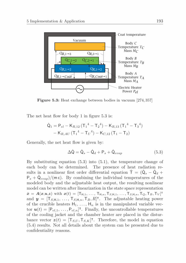
5 Implementation & Application 193
Figure 5.3: Heat exchange between bodies in vacuum [274,357]
The net heat flow for body 1 in figure 5.3 is:
Q1 = Pel − KR,12 (T14 − T2
4)− KR,13 (T14 − T3
4)
− KR,AU (T14 − TU
4)− KC,12 (T1 − T2)
Generally, the net heat flow is given by:
ΔQ = Qs − Qd + Ps + Qevap (5.3)
By substituting equation (5.3) into (5.1), the temperature change ofeach body can be determined. The presence of heat radiation re-sults in a nonlinear first order differential equation T = (Qs − Qd +Ps + Qevap)/(m c). By combining the individual temperatures of themodeled body and the adjustable heat output, the resulting nonlinearmodel can be written after linearization in the state space representationx = A(x,u,z) with x(t) = [TH,1, . . . , TH,n, TS,H,1, . . . , TS,H,n, TQ, TB , TV ]ᵀ
and y = [TS,H,1, . . . , TS,H,n, TB , R]ᵀ. The adjustable heating powerof the crucible heaters H1, . . . , Hn is in the manipulated variable vec-tor u(t) = [Pel,1, . . . , Pel,n]ᵀ. Finally, the uncontrollable temperaturesof the cooling jacket and the chamber heater are placed in the distur-bance vector z(t) = [TS,U , TS,K ]ᵀ. Therefore, the model in equation(5.4) results. Not all details about the system can be presented due toconfidentiality reasons.
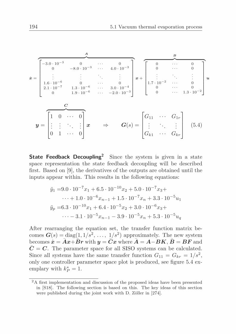
194 5.1 Vacuum thermal evaporation process
x =
A︷ ︸︸ ︷⎡⎢⎢⎢⎢⎢⎣−3.0 · 10−3 0 · · · 0
0 −8.0 · 10−3 · · · 4.0 · 10−3
......
. . ....
1.6 · 10−6 0 · · · 02.1 · 10−7 1.3 · 10−6 · · · 3.0 · 10−4
0 1.9 · 10−6 · · · −2.0 · 10−3
⎤⎥⎥⎥⎥⎥⎦x +
B︷ ︸︸ ︷⎡⎢⎢⎢⎢⎣0 · · · 00 · · · 0...
. . ....
1.7 · 10−2 · · · 00 · · · 00 · · · 1.3 · 10−2
⎤⎥⎥⎥⎥⎦u
y =
C︷ ︸︸ ︷⎡⎢⎢⎣1 0 · · · 0...
.... . .
...0 1 · · · 0
⎤⎥⎥⎦x ⇒ G(s) =
⎡⎢⎢⎣G11 · · · G1r
.... . .
...Gk1 · · · Gkr
⎤⎥⎥⎦ (5.4)
State Feedback Decoupling2 Since the system is given in a statespace representation the state feedback decoupling will be describedfirst. Based on [9], the derivatives of the outputs are obtained until theinputs appear within. This results in the following equations:
y1 =9.0 · 10−7x1 + 6.5 · 10−10x2 + 5.0 · 10−7x3+· · ·+ 1.0 · 10−6xn−1 + 1.5 · 10−7xn + 3.3 · 10−5u1
yp =6.3 · 10−10x1 + 6.4 · 10−5x2 + 3.0 · 10−6x3+· · · − 3.1 · 10−5xn−1 − 3.9 · 10−5xn + 5.3 · 10−5uq
After rearranging the equation set, the transfer function matrix be-comes G(s) = diag(1, 1/s2, . . . , 1/s2) approximately. The new systembecomes x = Ax+Br with y = Cx where A = A−BK, B = BF andC = C. The parameter space for all SISO systems can be calculated.Since all systems have the same transfer function G11 = Gkr = 1/s2,only one controller parameter space plot is produced, see figure 5.4 ex-emplary with k∗
P = 1.
2A first implementation and discussion of the proposed ideas have been presentedin [S18]. The following section is based on this. The key ideas of this sectionwere published during the joint work with D. Zöller in [274].
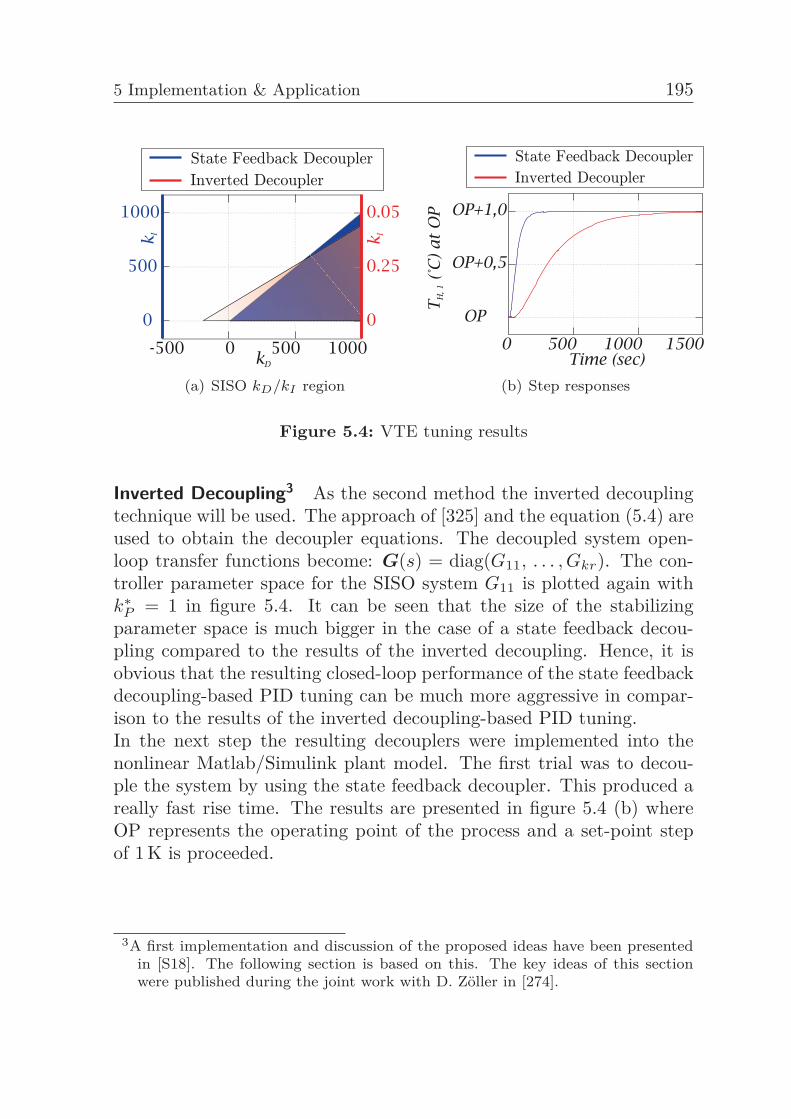
5 Implementation & Application 195
(a) SISO kD/kI region (b) Step responses
Figure 5.4: VTE tuning results
Inverted Decoupling3 As the second method the inverted decouplingtechnique will be used. The approach of [325] and the equation (5.4) areused to obtain the decoupler equations. The decoupled system open-loop transfer functions become: G(s) = diag(G11, . . . , Gkr). The con-troller parameter space for the SISO system G11 is plotted again withk∗
P = 1 in figure 5.4. It can be seen that the size of the stabilizingparameter space is much bigger in the case of a state feedback decou-pling compared to the results of the inverted decoupling. Hence, it isobvious that the resulting closed-loop performance of the state feedbackdecoupling-based PID tuning can be much more aggressive in compar-ison to the results of the inverted decoupling-based PID tuning.In the next step the resulting decouplers were implemented into thenonlinear Matlab/Simulink plant model. The first trial was to decou-ple the system by using the state feedback decoupler. This produced areally fast rise time. The results are presented in figure 5.4 (b) whereOP represents the operating point of the process and a set-point stepof 1 K is proceeded.
3A first implementation and discussion of the proposed ideas have been presentedin [S18]. The following section is based on this. The key ideas of this sectionwere published during the joint work with D. Zöller in [274].
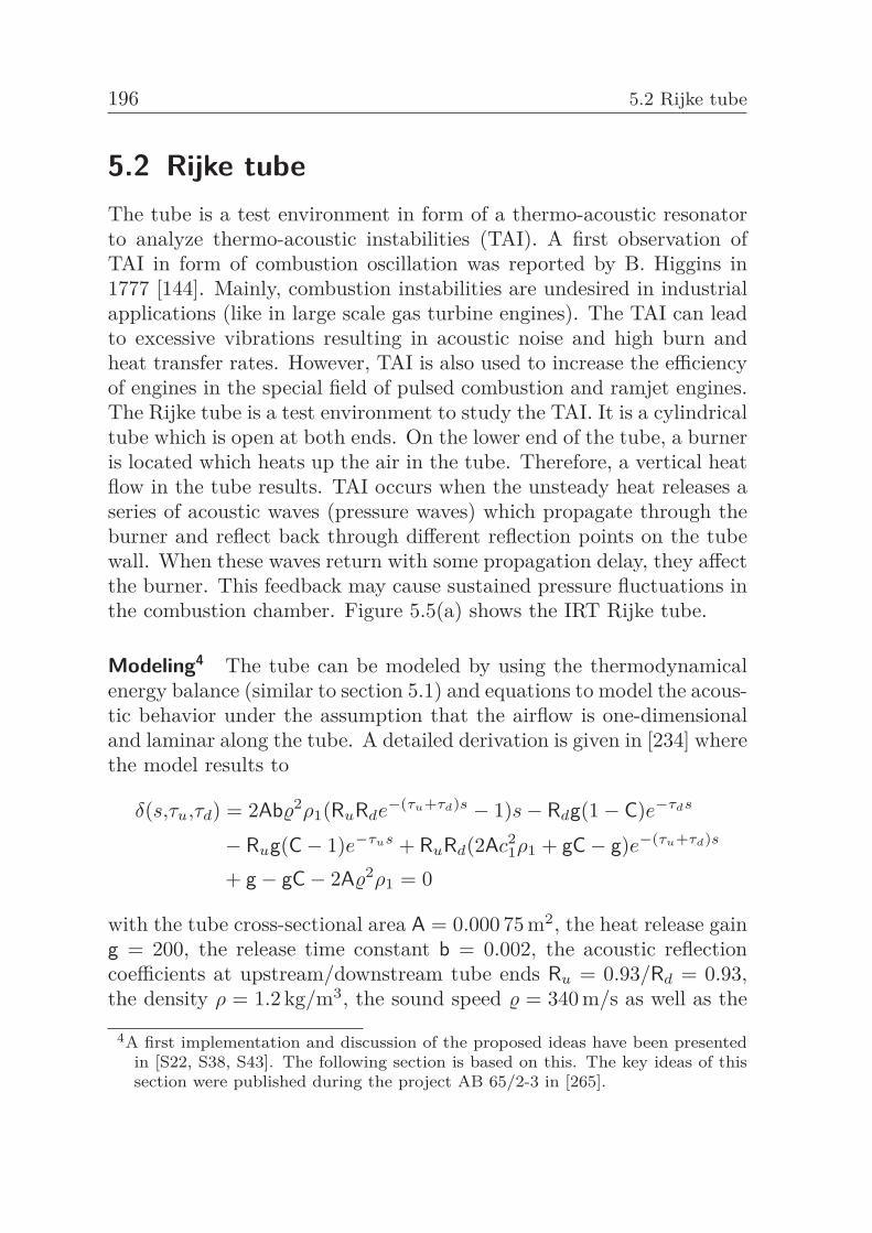
196 5.2 Rijke tube
5.2 Rijke tubeThe tube is a test environment in form of a thermo-acoustic resonatorto analyze thermo-acoustic instabilities (TAI). A first observation ofTAI in form of combustion oscillation was reported by B. Higgins in1777 [144]. Mainly, combustion instabilities are undesired in industrialapplications (like in large scale gas turbine engines). The TAI can leadto excessive vibrations resulting in acoustic noise and high burn andheat transfer rates. However, TAI is also used to increase the efficiencyof engines in the special field of pulsed combustion and ramjet engines.The Rijke tube is a test environment to study the TAI. It is a cylindricaltube which is open at both ends. On the lower end of the tube, a burneris located which heats up the air in the tube. Therefore, a vertical heatflow in the tube results. TAI occurs when the unsteady heat releases aseries of acoustic waves (pressure waves) which propagate through theburner and reflect back through different reflection points on the tubewall. When these waves return with some propagation delay, they affectthe burner. This feedback may cause sustained pressure fluctuations inthe combustion chamber. Figure 5.5(a) shows the IRT Rijke tube.
Modeling4 The tube can be modeled by using the thermodynamicalenergy balance (similar to section 5.1) and equations to model the acous-tic behavior under the assumption that the airflow is one-dimensionaland laminar along the tube. A detailed derivation is given in [234] wherethe model results to
δ(s,τu,τd) = 2Ab�2ρ1(RuRde−(τu+τd)s − 1)s− Rdg(1− C)e−τds
− Rug(C− 1)e−τus + RuRd(2Ac21ρ1 + gC− g)e−(τu+τd)s
+ g − gC− 2A�2ρ1 = 0
with the tube cross-sectional area A = 0.000 75 m2, the heat release gaing = 200, the release time constant b = 0.002, the acoustic reflectioncoefficients at upstream/downstream tube ends Ru = 0.93/Rd = 0.93,the density ρ = 1.2 kg/m3, the sound speed � = 340 m/s as well as the
4A first implementation and discussion of the proposed ideas have been presentedin [S22, S38, S43]. The following section is based on this. The key ideas of thissection were published during the project AB 65/2-3 in [265].
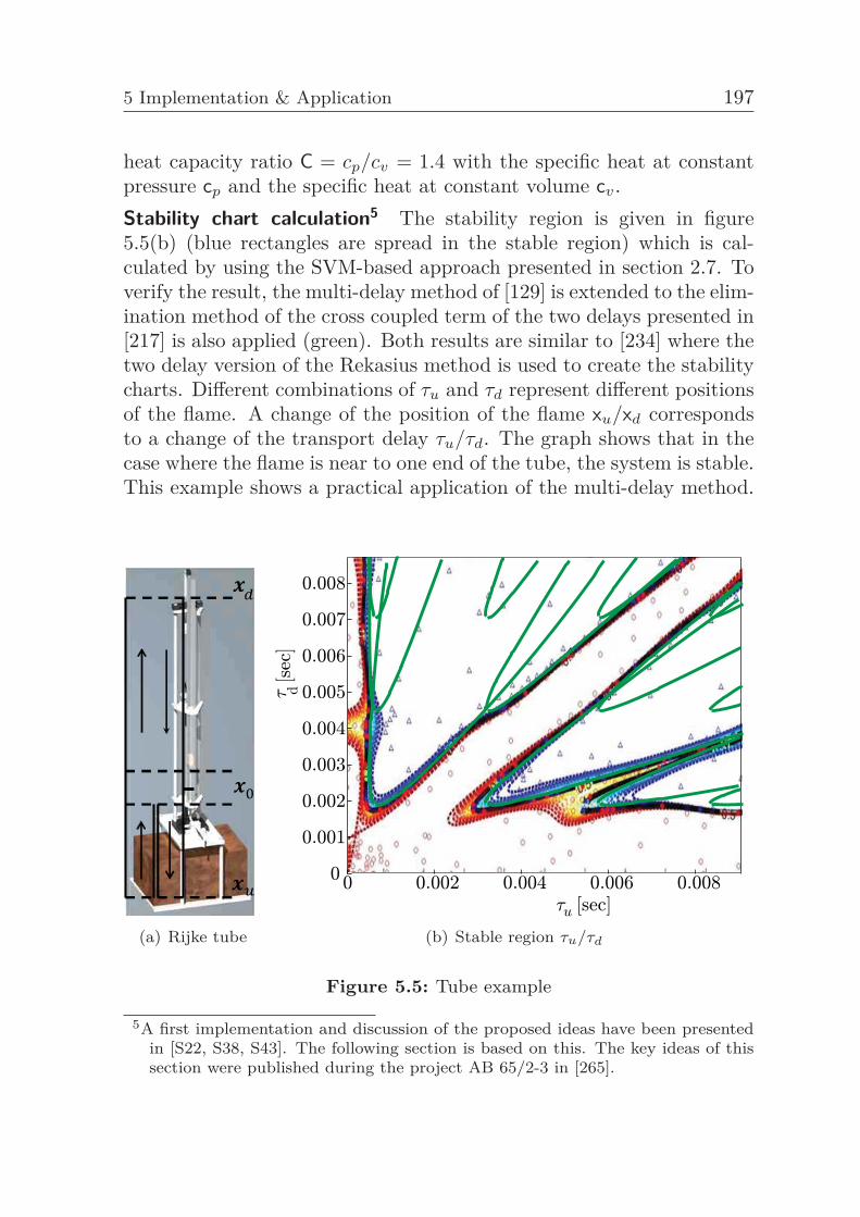
5 Implementation & Application 197
heat capacity ratio C = cp/cv = 1.4 with the specific heat at constantpressure cp and the specific heat at constant volume cv.Stability chart calculation5 The stability region is given in figure5.5(b) (blue rectangles are spread in the stable region) which is cal-culated by using the SVM-based approach presented in section 2.7. Toverify the result, the multi-delay method of [129] is extended to the elim-ination method of the cross coupled term of the two delays presented in[217] is also applied (green). Both results are similar to [234] where thetwo delay version of the Rekasius method is used to create the stabilitycharts. Different combinations of τu and τd represent different positionsof the flame. A change of the position of the flame xu/xd correspondsto a change of the transport delay τu/τd. The graph shows that in thecase where the flame is near to one end of the tube, the system is stable.This example shows a practical application of the multi-delay method.
(a) Rijke tube (b) Stable region τu/τd
Figure 5.5: Tube example
5A first implementation and discussion of the proposed ideas have been presentedin [S22, S38, S43]. The following section is based on this. The key ideas of thissection were published during the project AB 65/2-3 in [265].
198 5.3 Ventricular assist device
5.3 Ventricular assist deviceApproximately 30 million people suffer from advanced or terminal heartfailures worldwide. This is often a deadly disease where the myocardiumis damaged in such way that it cannot provide sufficient cardiovascularsupport. The transplantation of a donor heart is the current gold stan-dard for the treatment of terminal heart failures. With an incidenceof 2 million and an ongoing steady decrease of donor hearts [99], theneed for an alternative therapy increases. Most often ventricular as-sist devices (VAD) are applied to relieve the heart and give a sufficientcardiovascular support [204]. VADs are blood-pumps which exist in var-ious implantable and extra-corporal hardware implementations. Theyare connected parallel to the damaged ventricle leaving the heart intact(as opposed to artificial heart devices). VADs can be used either for abridge-to-transplant therapy until a suitable donor organ is available oras a destination therapy for a life-long support. The newest researchfocuses on a third option, the bridge-to-recovery therapy. Studies sug-gest that for some patients with a VAD support, the left ventricle couldfinally recover from its damage. In some cases, after a temporal supportthe heart managed the recovery (reverse modeling of cellular damage)and a gradual tapering of the VAD support (weaning) was successful.Those cases motivate research for an optimal profile of relief of ventricu-lar load and a control strategy to realize this profile. In this context, thefollowing section deals with the robust controller synthesis for a VAD.The used continuous flow VAD is a deltastream® DP3 from medos®.
Modeling6 An appropriate model of the VAD is needed in order tomatch the robustness specifications of the controller. Therefore, a gray-box system identification for the VAD is used. Starting from the char-acteristic chart the following characteristic equation is used to describethe pressure difference between the in- and outlet of the VAD as a func-tion of the flow and the rotational speed, see [304]: Δp = a1Vvad_stat +a2V 2
vad_stat + a3ω2. The flow Vvad_stat represents the stationary flowthrough the VAD, Δp is the pressure difference across the VAD and ω
6A first implementation and discussion of the proposed ideas have been presentedin [S11, S20, S23, S24, S25, S33, S34, S35, S36, S42, S44]. The following sectionis based on this. The key ideas of this section were published during the projectAB 65/2-3 in [135,272].
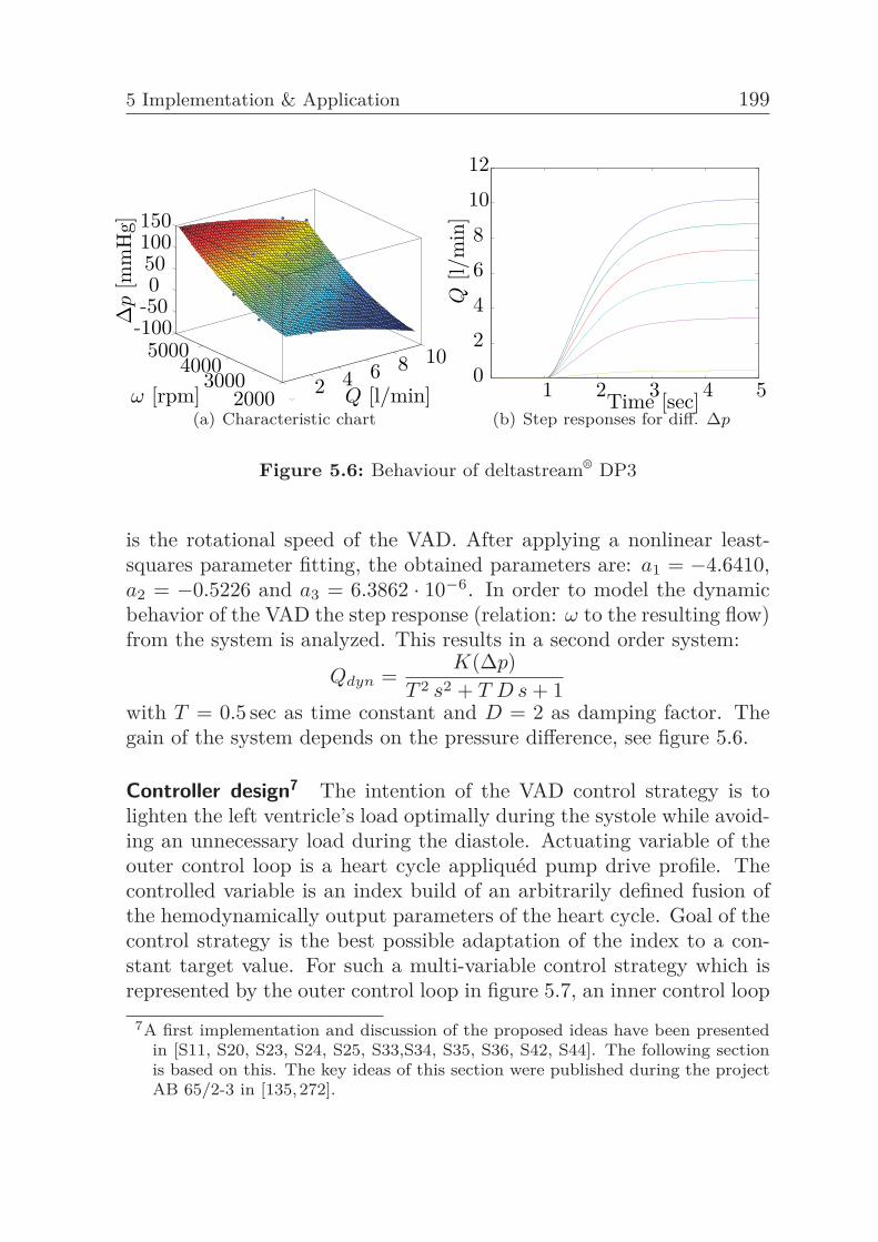
5 Implementation & Application 199
0 2 4 6 8 10
20003000
40005000
-100-50050100150
Q [l/min]ω [rpm]
Δp
[mm
Hg]
(a) Characteristic chart
0 1 2 3 4 50
2
4
6
8
10
12
Time [sec]
Q[l/
min
]
(b) Step responses for diff. Δp
Figure 5.6: Behaviour of deltastream® DP3
is the rotational speed of the VAD. After applying a nonlinear least-squares parameter fitting, the obtained parameters are: a1 = −4.6410,a2 = −0.5226 and a3 = 6.3862 · 10−6. In order to model the dynamicbehavior of the VAD the step response (relation: ω to the resulting flow)from the system is analyzed. This results in a second order system:
Qdyn =K(Δp)
T 2 s2 + T D s + 1with T = 0.5 sec as time constant and D = 2 as damping factor. Thegain of the system depends on the pressure difference, see figure 5.6.
Controller design7 The intention of the VAD control strategy is tolighten the left ventricle’s load optimally during the systole while avoid-ing an unnecessary load during the diastole. Actuating variable of theouter control loop is a heart cycle appliquéd pump drive profile. Thecontrolled variable is an index build of an arbitrarily defined fusion ofthe hemodynamically output parameters of the heart cycle. Goal of thecontrol strategy is the best possible adaptation of the index to a con-stant target value. For such a multi-variable control strategy which isrepresented by the outer control loop in figure 5.7, an inner control loop
7A first implementation and discussion of the proposed ideas have been presentedin [S11, S20, S23, S24, S25, S33,S34, S35, S36, S42, S44]. The following sectionis based on this. The key ideas of this section were published during the projectAB 65/2-3 in [135,272].
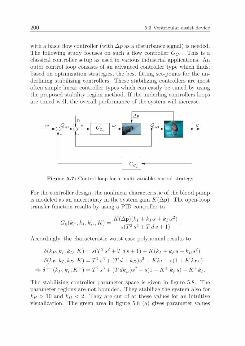
200 5.3 Ventricular assist device
with a basic flow controller (with Δp as a disturbance signal) is needed.The following study focuses on such a flow controller GC1 . This is aclassical controller setup as used in various industrial applications. Anouter control loop consists of an advanced controller type which finds,based on optimization strategies, the best fitting set-points for the un-derlining stabilizing controllers. These stabilizing controllers are mostoften simple linear controller types which can easily be tuned by usingthe proposed stability region method. If the underling controllers loopsare tuned well, the overall performance of the system will increase.
Figure 5.7: Control loop for a multi-variable control strategy
For the controller design, the nonlinear characteristic of the blood pumpis modeled as an uncertainty in the system gain K(Δp). The open-looptransfer function results by using a PID controller to
G0(kP , kI , kD, K) =K(Δp)(kI + kP s + kDs2)
s(T 2 s2 + T d s + 1).
Accordingly, the characteristic worst case polynomial results to
δ(kP , kI , kD, K) = s(T 2 s2 + T d s + 1) + K(kI + kP s + kDs2)δ(kP , kI , kD, K) = T 2 s3 + (T d + kD)s2 + KkI + s(1 + K kP s)
⇒ δ+−(kP , kI , K+) = T 2 s3 + (T dkD)s2 + s(1 + K+ kP s) + K+kI .
The stabilizing controller parameter space is given in figure 5.8. Theparameter regions are not bounded. They stabilize the system also forkP > 10 and kD < 2. They are cut of at these values for an intuitivevisualization. The green area in figure 5.8 (a) gives parameter values
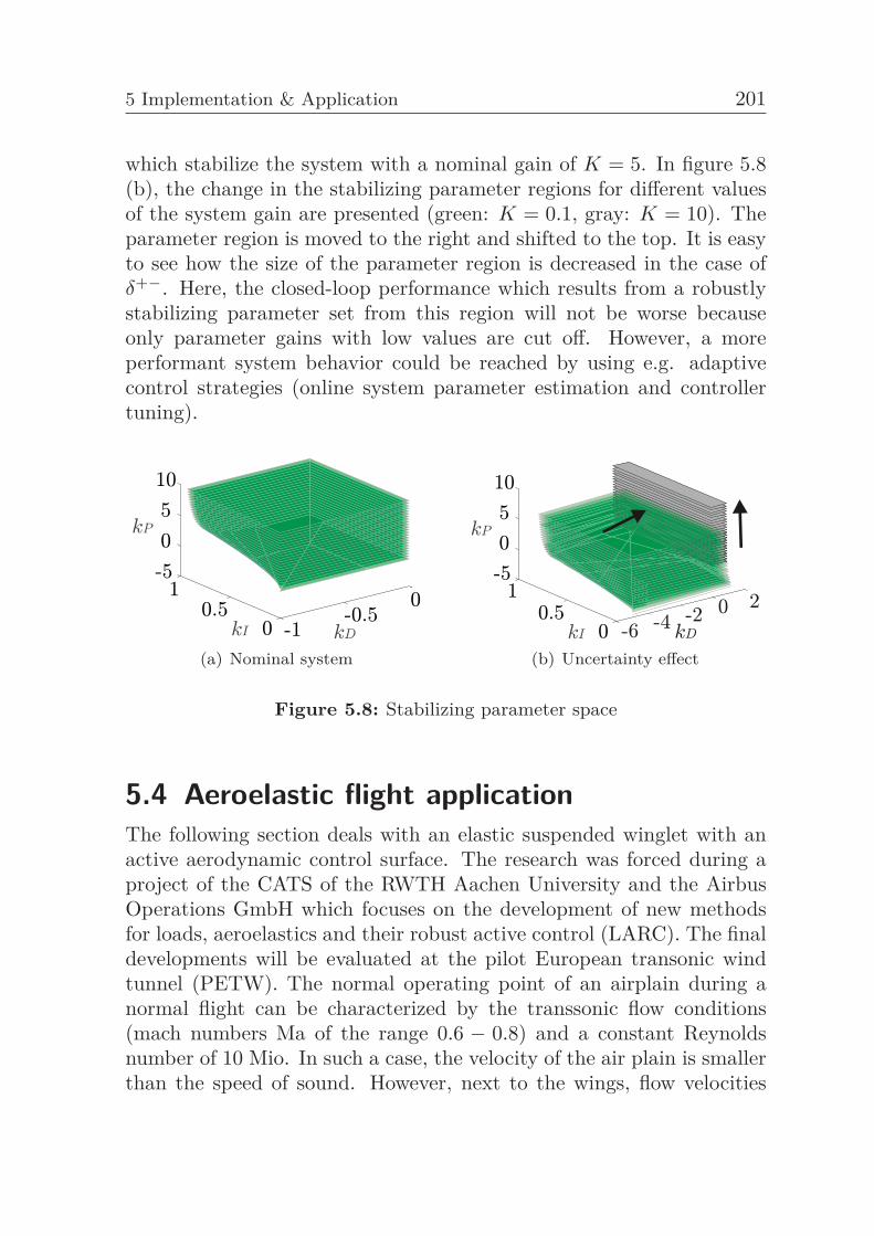
5 Implementation & Application 201
which stabilize the system with a nominal gain of K = 5. In figure 5.8(b), the change in the stabilizing parameter regions for different valuesof the system gain are presented (green: K = 0.1, gray: K = 10). Theparameter region is moved to the right and shifted to the top. It is easyto see how the size of the parameter region is decreased in the case ofδ+−. Here, the closed-loop performance which results from a robustlystabilizing parameter set from this region will not be worse becauseonly parameter gains with low values are cut off. However, a moreperformant system behavior could be reached by using e.g. adaptivecontrol strategies (online system parameter estimation and controllertuning).
(a) Nominal system (b) Uncertainty effect
Figure 5.8: Stabilizing parameter space
5.4 Aeroelastic flight applicationThe following section deals with an elastic suspended winglet with anactive aerodynamic control surface. The research was forced during aproject of the CATS of the RWTH Aachen University and the AirbusOperations GmbH which focuses on the development of new methodsfor loads, aeroelastics and their robust active control (LARC). The finaldevelopments will be evaluated at the pilot European transonic windtunnel (PETW). The normal operating point of an airplain during anormal flight can be characterized by the transsonic flow conditions(mach numbers Ma of the range 0.6 − 0.8) and a constant Reynoldsnumber of 10 Mio. In such a case, the velocity of the air plain is smallerthan the speed of sound. However, next to the wings, flow velocities
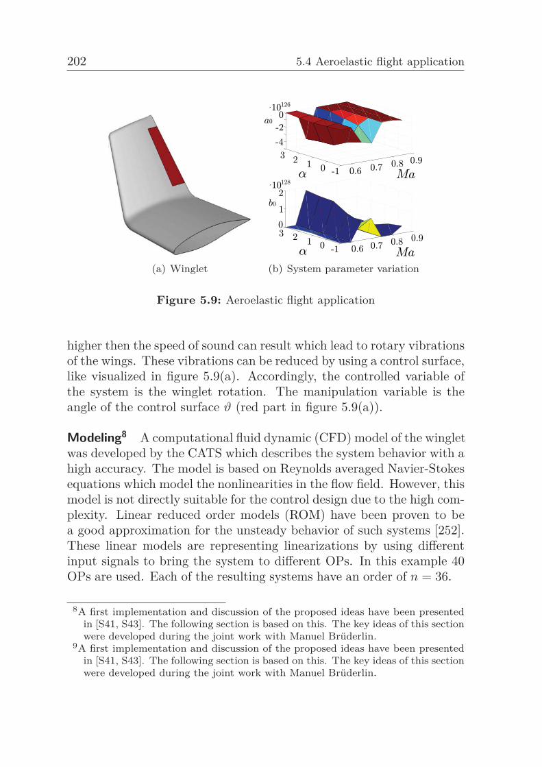
202 5.4 Aeroelastic flight application
(a) Winglet (b) System parameter variation
Figure 5.9: Aeroelastic flight application
higher then the speed of sound can result which lead to rotary vibrationsof the wings. These vibrations can be reduced by using a control surface,like visualized in figure 5.9(a). Accordingly, the controlled variable ofthe system is the winglet rotation. The manipulation variable is theangle of the control surface ϑ (red part in figure 5.9(a)).
Modeling8 A computational fluid dynamic (CFD) model of the wingletwas developed by the CATS which describes the system behavior with ahigh accuracy. The model is based on Reynolds averaged Navier-Stokesequations which model the nonlinearities in the flow field. However, thismodel is not directly suitable for the control design due to the high com-plexity. Linear reduced order models (ROM) have been proven to bea good approximation for the unsteady behavior of such systems [252].These linear models are representing linearizations by using differentinput signals to bring the system to different OPs. In this example 40OPs are used. Each of the resulting systems have an order of n = 36.
8A first implementation and discussion of the proposed ideas have been presentedin [S41, S43]. The following section is based on this. The key ideas of this sectionwere developed during the joint work with Manuel Brüderlin.
9A first implementation and discussion of the proposed ideas have been presentedin [S41, S43]. The following section is based on this. The key ideas of this sectionwere developed during the joint work with Manuel Brüderlin.
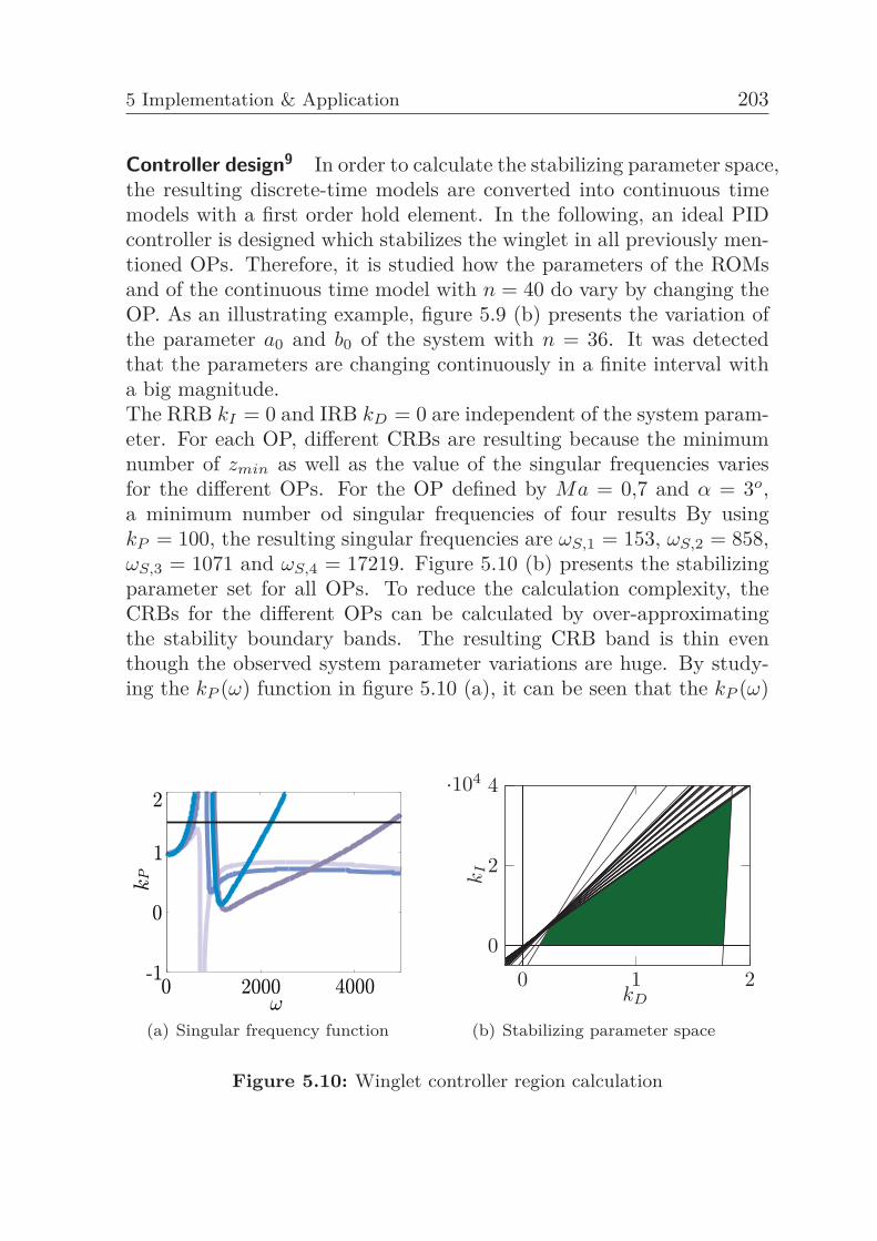
5 Implementation & Application 203
Controller design9 In order to calculate the stabilizing parameter space,the resulting discrete-time models are converted into continuous timemodels with a first order hold element. In the following, an ideal PIDcontroller is designed which stabilizes the winglet in all previously men-tioned OPs. Therefore, it is studied how the parameters of the ROMsand of the continuous time model with n = 40 do vary by changing theOP. As an illustrating example, figure 5.9 (b) presents the variation ofthe parameter a0 and b0 of the system with n = 36. It was detectedthat the parameters are changing continuously in a finite interval witha big magnitude.The RRB kI = 0 and IRB kD = 0 are independent of the system param-eter. For each OP, different CRBs are resulting because the minimumnumber of zmin as well as the value of the singular frequencies variesfor the different OPs. For the OP defined by Ma = 0,7 and α = 3o,a minimum number od singular frequencies of four results By usingkP = 100, the resulting singular frequencies are ωS,1 = 153, ωS,2 = 858,ωS,3 = 1071 and ωS,4 = 17219. Figure 5.10 (b) presents the stabilizingparameter set for all OPs. To reduce the calculation complexity, theCRBs for the different OPs can be calculated by over-approximatingthe stability boundary bands. The resulting CRB band is thin eventhough the observed system parameter variations are huge. By study-ing the kP (ω) function in figure 5.10 (a), it can be seen that the kP (ω)
(a) Singular frequency function
kI
kD
·104
0 1 20
2
4
(b) Stabilizing parameter space
Figure 5.10: Winglet controller region calculation
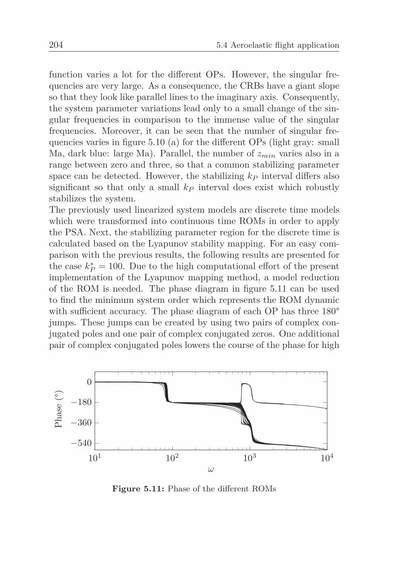
204 5.4 Aeroelastic flight application
function varies a lot for the different OPs. However, the singular fre-quencies are very large. As a consequence, the CRBs have a giant slopeso that they look like parallel lines to the imaginary axis. Consequently,the system parameter variations lead only to a small change of the sin-gular frequencies in comparison to the immense value of the singularfrequencies. Moreover, it can be seen that the number of singular fre-quencies varies in figure 5.10 (a) for the different OPs (light gray: smallMa, dark blue: large Ma). Parallel, the number of zmin varies also in arange between zero and three, so that a common stabilizing parameterspace can be detected. However, the stabilizing kP interval differs alsosignificant so that only a small kP interval does exist which robustlystabilizes the system.The previously used linearized system models are discrete time modelswhich were transformed into continuous time ROMs in order to applythe PSA. Next, the stabilizing parameter region for the discrete time iscalculated based on the Lyapunov stability mapping. For an easy com-parison with the previous results, the following results are presented forthe case k∗
P = 100. Due to the high computational effort of the presentimplementation of the Lyapunov mapping method, a model reductionof the ROM is needed. The phase diagram in figure 5.11 can be usedto find the minimum system order which represents the ROM dynamicwith sufficient accuracy. The phase diagram of each OP has three 180°jumps. These jumps can be created by using two pairs of complex con-jugated poles and one pair of complex conjugated zeros. One additionalpair of complex conjugated poles lowers the course of the phase for high
Pha
se(°
)
101 102 103 104
−540
−360
−180
0
ω
Figure 5.11: Phase of the different ROMs
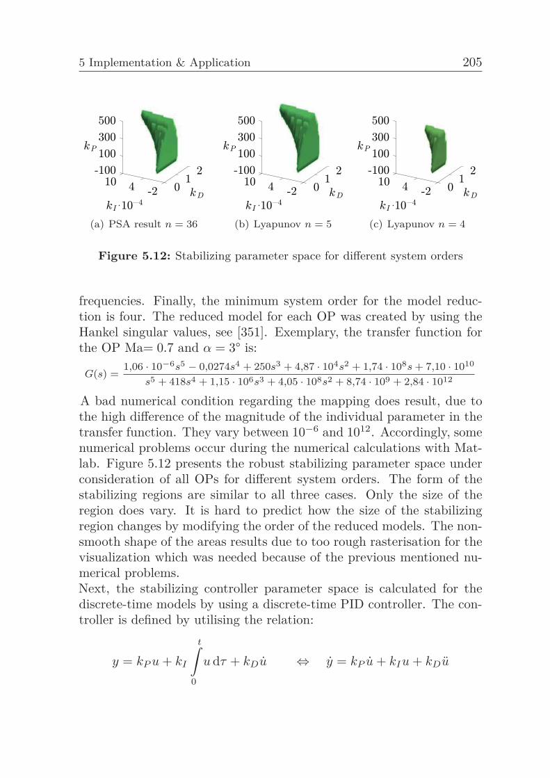
5 Implementation & Application 205
(a) PSA result n = 36 (b) Lyapunov n = 5 (c) Lyapunov n = 4
Figure 5.12: Stabilizing parameter space for different system orders
frequencies. Finally, the minimum system order for the model reduc-tion is four. The reduced model for each OP was created by using theHankel singular values, see [351]. Exemplary, the transfer function forthe OP Ma= 0.7 and α = 3° is:
G(s) =1,06 · 10−6s5 − 0,0274s4 + 250s3 + 4,87 · 104s2 + 1,74 · 108s + 7,10 · 1010
s5 + 418s4 + 1,15 · 106s3 + 4,05 · 108s2 + 8,74 · 109 + 2,84 · 1012
A bad numerical condition regarding the mapping does result, due tothe high difference of the magnitude of the individual parameter in thetransfer function. They vary between 10−6 and 1012. Accordingly, somenumerical problems occur during the numerical calculations with Mat-lab. Figure 5.12 presents the robust stabilizing parameter space underconsideration of all OPs for different system orders. The form of thestabilizing regions are similar to all three cases. Only the size of theregion does vary. It is hard to predict how the size of the stabilizingregion changes by modifying the order of the reduced models. The non-smooth shape of the areas results due to too rough rasterisation for thevisualization which was needed because of the previous mentioned nu-merical problems.Next, the stabilizing controller parameter space is calculated for thediscrete-time models by using a discrete-time PID controller. The con-troller is defined by utilising the relation:
y = kP u + kI
t∫0
u dτ + kDu ⇔ y = kP u + kIu + kDu
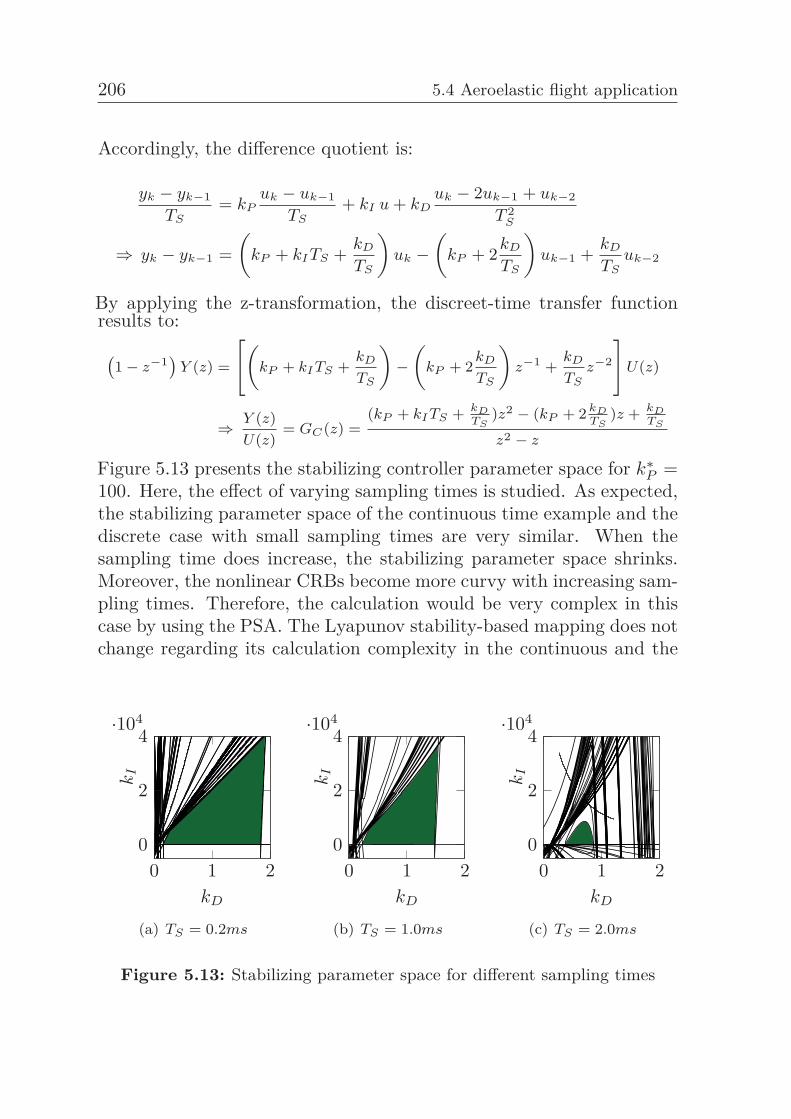
206 5.4 Aeroelastic flight application
Accordingly, the difference quotient is:
yk − yk−1
TS= kP
uk − uk−1
TS+ kI u + kD
uk − 2uk−1 + uk−2
T 2S
⇒ yk − yk−1 =(
kP + kITS + kD
TS
)uk −
(kP + 2kD
TS
)uk−1 + kD
TSuk−2
By applying the z-transformation, the discreet-time transfer functionresults to:(
1 − z−1)
Y (z) =
[(kP + kITS +
kD
TS
)−(
kP + 2kD
TS
)z−1 +
kD
TSz−2
]U(z)
⇒ Y (z)U(z)
= GC(z) =(kP + kITS + kD
TS)z2 − (kP + 2 kD
TS)z + kD
TS
z2 − z
Figure 5.13 presents the stabilizing controller parameter space for k∗P =
100. Here, the effect of varying sampling times is studied. As expected,the stabilizing parameter space of the continuous time example and thediscrete case with small sampling times are very similar. When thesampling time does increase, the stabilizing parameter space shrinks.Moreover, the nonlinear CRBs become more curvy with increasing sam-pling times. Therefore, the calculation would be very complex in thiscase by using the PSA. The Lyapunov stability-based mapping does notchange regarding its calculation complexity in the continuous and the
kI
·104
0 1 20
2
4
kD
(a) TS = 0.2ms
kI
·104
0 1 20
2
4
kD
(b) TS = 1.0ms
kI
·104
0 1 20
2
4
kD
(c) TS = 2.0ms
Figure 5.13: Stabilizing parameter space for different sampling times
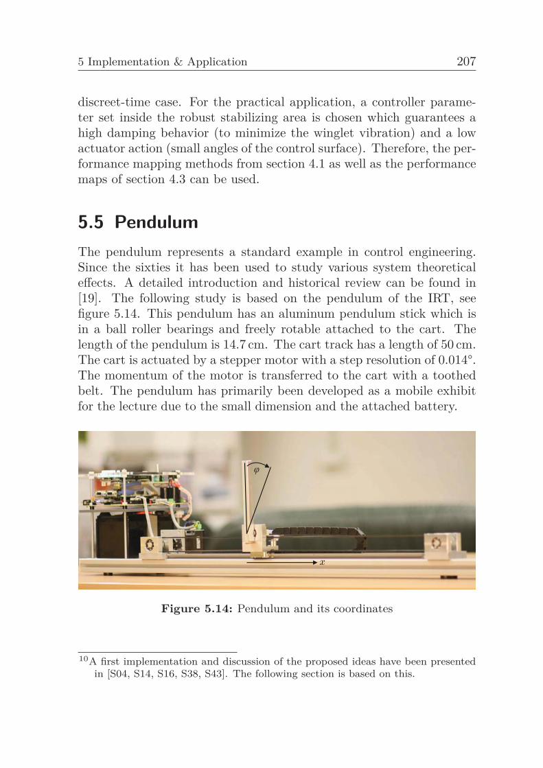
5 Implementation & Application 207
discreet-time case. For the practical application, a controller parame-ter set inside the robust stabilizing area is chosen which guarantees ahigh damping behavior (to minimize the winglet vibration) and a lowactuator action (small angles of the control surface). Therefore, the per-formance mapping methods from section 4.1 as well as the performancemaps of section 4.3 can be used.
5.5 PendulumThe pendulum represents a standard example in control engineering.Since the sixties it has been used to study various system theoreticaleffects. A detailed introduction and historical review can be found in[19]. The following study is based on the pendulum of the IRT, seefigure 5.14. This pendulum has an aluminum pendulum stick which isin a ball roller bearings and freely rotable attached to the cart. Thelength of the pendulum is 14.7 cm. The cart track has a length of 50 cm.The cart is actuated by a stepper motor with a step resolution of 0.014°.The momentum of the motor is transferred to the cart with a toothedbelt. The pendulum has primarily been developed as a mobile exhibitfor the lecture due to the small dimension and the attached battery.
Figure 5.14: Pendulum and its coordinates
10A first implementation and discussion of the proposed ideas have been presentedin [S04, S14, S16, S38, S43]. The following section is based on this.
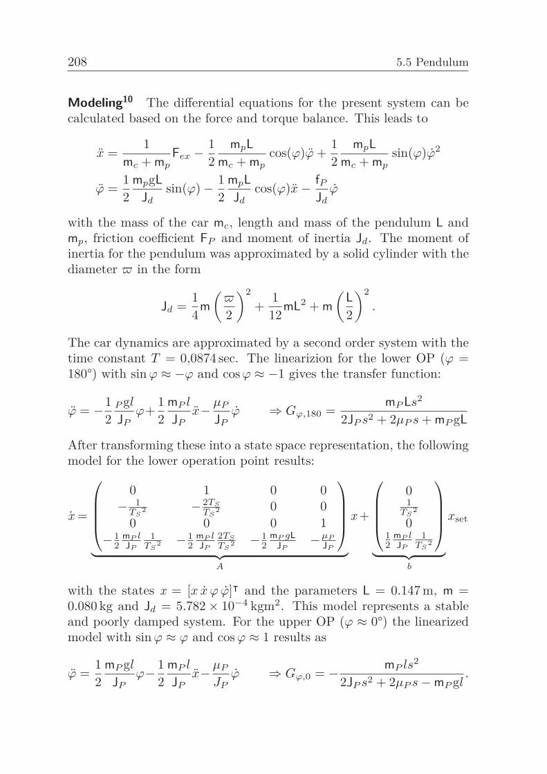
208 5.5 Pendulum
Modeling10 The differential equations for the present system can becalculated based on the force and torque balance. This leads to
x =1
mc + mpFex −
12
mpLmc + mp
cos(ϕ)ϕ +12
mpLmc + mp
sin(ϕ)ϕ2
ϕ =12
mpgLJd
sin(ϕ)− 12
mpLJd
cos(ϕ)x− fPJd
ϕ
with the mass of the car mc, length and mass of the pendulum L andmp, friction coefficient FP and moment of inertia Jd. The moment ofinertia for the pendulum was approximated by a solid cylinder with thediameter � in the form
Jd =14
m(
�
2
)2+
112
mL2 + m(
L2
)2.
The car dynamics are approximated by a second order system with thetime constant T = 0,0874 sec. The linearizion for the lower OP (ϕ =180°) with sin ϕ ≈ −ϕ and cos ϕ ≈ −1 gives the transfer function:
ϕ = −12
P gl
JPϕ+
12
mP l
JPx− μP
JPϕ ⇒ Gϕ,180 =
mP Ls2
2JP s2 + 2μP s + mP gL
After transforming these into a state space representation, the followingmodel for the lower operation point results:
x =
⎛⎜⎜⎜⎝0 1 0 0− 1
TS2 − 2TS
TS2 0 0
0 0 0 1− 1
2mP lJP
1TS
2 − 12
mP lJP
2TS
TS2 − 1
2mP gL
JP−μP
JP
⎞⎟⎟⎟⎠︸ ︷︷ ︸
A
x +
⎛⎜⎜⎜⎝01
TS2
012
mP lJP
1TS
2
⎞⎟⎟⎟⎠︸ ︷︷ ︸
b
xset
with the states x = [x x ϕ ϕ]ᵀ and the parameters L = 0.147 m, m =0.080 kg and Jd = 5.782× 10⁻⁴ kgm2. This model represents a stableand poorly damped system. For the upper OP (ϕ ≈ 0°) the linearizedmodel with sin ϕ ≈ ϕ and cos ϕ ≈ 1 results as
ϕ =12
mP gl
JPϕ− 1
2mP l
JPx− μP
JPϕ ⇒ Gϕ,0 = − mP ls2
2JP s2 + 2μP s−mP gl.
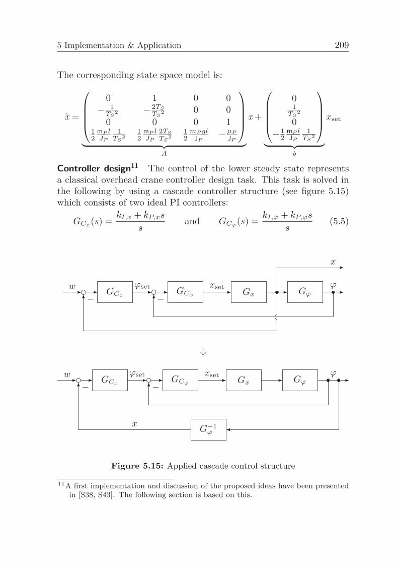
5 Implementation & Application 209
The corresponding state space model is:
x =
⎛⎜⎜⎜⎝0 1 0 0− 1
TS2 − 2TS
TS2 0 0
0 0 0 112
mP lJP
1TS
212
mP lJP
2TS
TS2
12
mP glJP
−μP
JP
⎞⎟⎟⎟⎠︸ ︷︷ ︸
A
x +
⎛⎜⎜⎜⎝01
TS2
0− 1
2mP lJP
1TS
2
⎞⎟⎟⎟⎠︸ ︷︷ ︸
b
xset
Controller design11 The control of the lower steady state representsa classical overhead crane controller design task. This task is solved inthe following by using a cascade controller structure (see figure 5.15)which consists of two ideal PI controllers:
GCx(s) =
kI,x + kP,xs
sand GCϕ
(s) =kI,ϕ + kP,ϕs
s(5.5)
wGCx
ϕsetGCϕ
xsetGx Gϕ
ϕ
x
− −
⇓
wGCx
ϕsetGCϕ
xsetGx Gϕ
ϕ
G−1ϕ
x
− −
Figure 5.15: Applied cascade control structure
11A first implementation and discussion of the proposed ideas have been presentedin [S38, S43]. The following section is based on this.
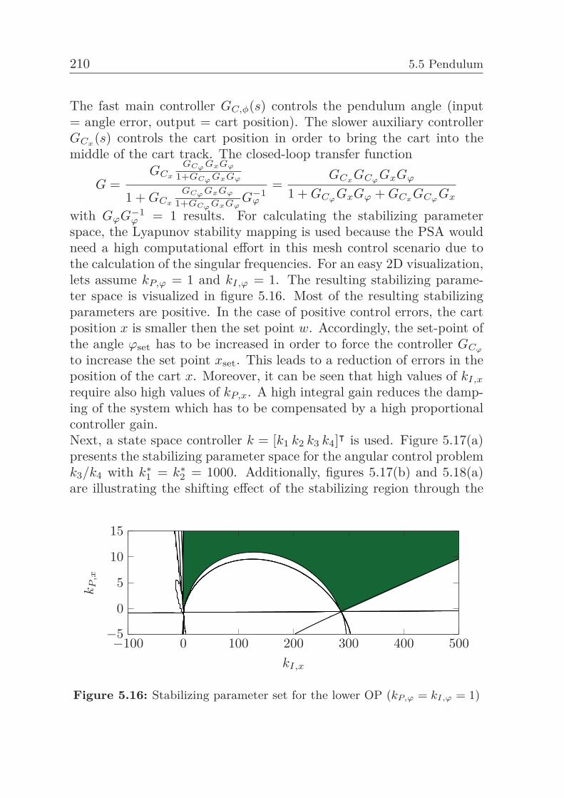
210 5.5 Pendulum
The fast main controller GC,φ(s) controls the pendulum angle (input= angle error, output = cart position). The slower auxiliary controllerGCx
(s) controls the cart position in order to bring the cart into themiddle of the cart track. The closed-loop transfer function
G =GCx
GCϕ GxGϕ
1+GCϕ GxGϕ
1 + GCx
GCϕ GxGϕ
1+GCϕ GxGϕG−1
ϕ
=GCx
GCϕGxGϕ
1 + GCϕGxGϕ + GCx
GCϕGx
with GϕG−1ϕ = 1 results. For calculating the stabilizing parameter
space, the Lyapunov stability mapping is used because the PSA wouldneed a high computational effort in this mesh control scenario due tothe calculation of the singular frequencies. For an easy 2D visualization,lets assume kP,ϕ = 1 and kI,ϕ = 1. The resulting stabilizing parame-ter space is visualized in figure 5.16. Most of the resulting stabilizingparameters are positive. In the case of positive control errors, the cartposition x is smaller then the set point w. Accordingly, the set-point ofthe angle ϕset has to be increased in order to force the controller GCϕ
to increase the set point xset. This leads to a reduction of errors in theposition of the cart x. Moreover, it can be seen that high values of kI,x
require also high values of kP,x. A high integral gain reduces the damp-ing of the system which has to be compensated by a high proportionalcontroller gain.Next, a state space controller k = [k1 k2 k3 k4]ᵀ is used. Figure 5.17(a)presents the stabilizing parameter space for the angular control problemk3/k4 with k∗
1 = k∗2 = 1000. Additionally, figures 5.17(b) and 5.18(a)
are illustrating the shifting effect of the stabilizing region through the
−100 0 100 200 300 400 500−5
0
5
10
15
kI,x
kP
,x
Figure 5.16: Stabilizing parameter set for the lower OP (kP,ϕ = kI,ϕ = 1)
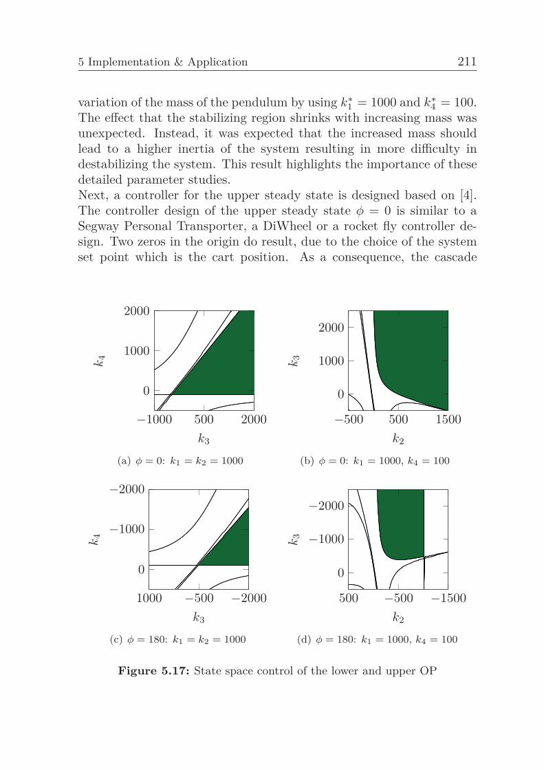
5 Implementation & Application 211
variation of the mass of the pendulum by using k∗1 = 1000 and k∗
4 = 100.The effect that the stabilizing region shrinks with increasing mass wasunexpected. Instead, it was expected that the increased mass shouldlead to a higher inertia of the system resulting in more difficulty indestabilizing the system. This result highlights the importance of thesedetailed parameter studies.Next, a controller for the upper steady state is designed based on [4].The controller design of the upper steady state φ = 0 is similar to aSegway Personal Transporter, a DiWheel or a rocket fly controller de-sign. Two zeros in the origin do result, due to the choice of the systemset point which is the cart position. As a consequence, the cascade
k4
−1000 500 2000
0
1000
2000
k3
(a) φ = 0: k1 = k2 = 1000
k3
−500 500 1500
0
1000
2000
k2
(b) φ = 0: k1 = 1000, k4 = 100
k4
1000 −500 −2000
0
−1000
−2000
k3
(c) φ = 180: k1 = k2 = 1000
k3
500 −500 −1500
0
−1000
−2000
k2
(d) φ = 180: k1 = 1000, k4 = 100
Figure 5.17: State space control of the lower and upper OP
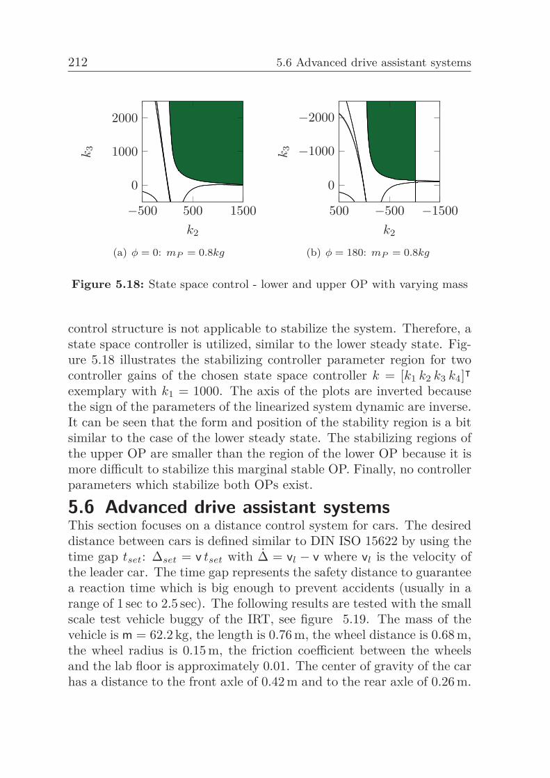
212 5.6 Advanced drive assistant systems
k3
−500 500 1500
0
1000
2000
k2
(a) φ = 0: mP = 0.8kg
k3
500 −500 −1500
0
−1000
−2000
k2
(b) φ = 180: mP = 0.8kg
Figure 5.18: State space control - lower and upper OP with varying mass
control structure is not applicable to stabilize the system. Therefore, astate space controller is utilized, similar to the lower steady state. Fig-ure 5.18 illustrates the stabilizing controller parameter region for twocontroller gains of the chosen state space controller k = [k1 k2 k3 k4]ᵀexemplary with k1 = 1000. The axis of the plots are inverted becausethe sign of the parameters of the linearized system dynamic are inverse.It can be seen that the form and position of the stability region is a bitsimilar to the case of the lower steady state. The stabilizing regions ofthe upper OP are smaller than the region of the lower OP because it ismore difficult to stabilize this marginal stable OP. Finally, no controllerparameters which stabilize both OPs exist.
5.6 Advanced drive assistant systemsThis section focuses on a distance control system for cars. The desireddistance between cars is defined similar to DIN ISO 15622 by using thetime gap tset: Δset = v tset with Δ = vl − v where vl is the velocity ofthe leader car. The time gap represents the safety distance to guaranteea reaction time which is big enough to prevent accidents (usually in arange of 1 sec to 2.5 sec). The following results are tested with the smallscale test vehicle buggy of the IRT, see figure 5.19. The mass of thevehicle is m = 62.2 kg, the length is 0.76 m, the wheel distance is 0.68 m,the wheel radius is 0.15 m, the friction coefficient between the wheelsand the lab floor is approximately 0.01. The center of gravity of the carhas a distance to the front axle of 0.42 m and to the rear axle of 0.26 m.
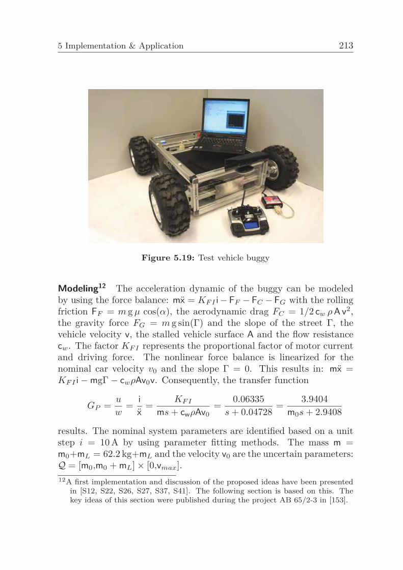
5 Implementation & Application 213
Figure 5.19: Test vehicle buggy
Modeling12 The acceleration dynamic of the buggy can be modeledby using the force balance: mx = KF I i− FF − FC − FG with the rollingfriction FF = m g μ cos(α), the aerodynamic drag FC = 1/2 cw ρ A v2,the gravity force FG = m g sin(Γ) and the slope of the street Γ, thevehicle velocity v, the stalled vehicle surface A and the flow resistancecw. The factor KF I represents the proportional factor of motor currentand driving force. The nonlinear force balance is linearized for thenominal car velocity v0 and the slope Γ = 0. This results in: mx =KF I i−mgΓ− cwρAv0v. Consequently, the transfer function
GP =u
w=
ix
=KF I
ms + cwρAv0=
0.06335s + 0.04728
=3.9404
m0s + 2.9408
results. The nominal system parameters are identified based on a unitstep i = 10 A by using parameter fitting methods. The mass m =m0+mL = 62.2 kg+mL and the velocity v0 are the uncertain parameters:Q = [m0,m0 + mL]× [0,vmax].12A first implementation and discussion of the proposed ideas have been presented
in [S12, S22, S26, S27, S37, S41]. The following section is based on this. Thekey ideas of this section were published during the project AB 65/2-3 in [153].
214 5.6 Advanced drive assistant systems
Robust distance controller design13 The distance control problemwas solved by using a PID controller. The resulting open-loop set pointtransfer function is
G0 =KF I
(kD s2 + kP s + kI
)s2(m s + cwρA v0) + KF I (kD s2 + kP s + kI)
.
Accordingly, the characteristic polynomial results in
δ(s,m,v0) = s2(ms + cwρAv0) + KF I
(kD s2 + kP s + kI
).
The uncertain parameters m and v0 are independent of each other.Therefore, the characteristic polynomial can be classified as an intervalpolynomial and it is sufficient to test the following Kharitonov polyno-mial for stability:
δ+−(s) = s2(m+s + cwρAv−0 ) + KF I
(kD s2 + kP s + kI
)= s3(m0 + mL) + KF I
(kD s2 + kP s + kI
)The RRB is kI = 0. An IRB doesn’t exist. The CRB is calculated by us-ing the PSA. Figure 5.20(a) presents the stabilizing controller parameterspace for the nominal system. For a first order system, no CRB exist.Consequently the parameter space is splitted into two regions separatedby the RRB and IRB. In this case, the parameter space is unbounded.This means, the system is also stable for kP < 0 : kI < −1, kD < −17and kP > 0 : kI > 1, kD > −14 as well as for kP < −50 and kP > 50.Figure 5.20(b) visualizes the effect of increasing the mass of the vehicleto the stability region (green: m = m0, gray: m = m0 + mL). It canbe seen, that the stability region is moving to the left. Therefore, thestability region is increased for kP > 0 and decreased for kP < 0. More-over, in figure 5.20(c) the effect by adding a small delay of 0.1 sec is pre-sented. In the delay case two IRBs exist, therefore the stability regionfor kD < −17 is eliminated. In addition, the delay produces three CRBsdue to the trigonometric functions in the CRB equations which resultsin the triangular stability region and a finite stabilizing kP interval. Inthe present example, the stability region shrinks by increasing the delay,13A first implementation and discussion of the proposed ideas have been presented
in [S12, S22, S26, S27, S37, S41]. The following section is based on this. Thekey ideas of this section were published during the project AB 65/2-3 in [153].
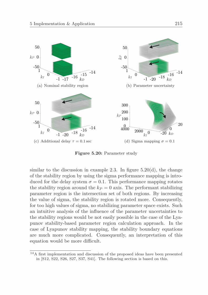
5 Implementation & Application 215
(a) Nominal stability region (b) Parameter uncertainty
(c) Additional delay τ = 0.1 sec (d) Sigma mapping σ = 0.1
Figure 5.20: Parameter study
similar to the discussion in example 2.3. In figure 5.20(d), the changeof the stability region by using the sigma performance mapping is intro-duced for the delay system σ = 0.1. This performance mapping rotatesthe stability region around the kP = 0 axis. The performant stabilizingparameter region is the intersection set of both regions. By increasingthe value of sigma, the stability region is rotated more. Consequently,for too high values of sigma, no stabilizing parameter space exists. Suchan intuitive analysis of the influence of the parameter uncertainties tothe stability regions would be not easily possible in the case of the Lya-punov stability-based parameter region calculation approach. In thecase of Lyapunov stability mapping, the stability boundary equationsare much more complicated. Consequently, an interpretation of thisequation would be more difficult.
14A first implementation and discussion of the proposed ideas have been presentedin [S12, S22, S26, S27, S37, S41]. The following section is based on this.
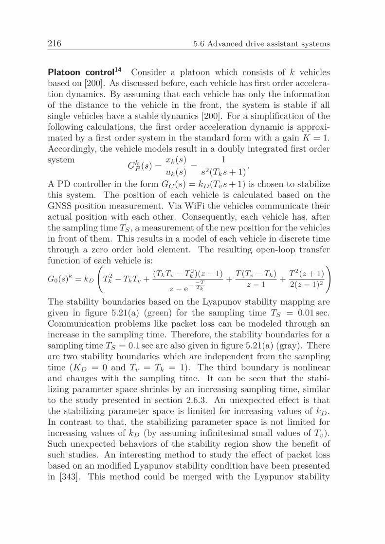
216 5.6 Advanced drive assistant systems
Platoon control14 Consider a platoon which consists of k vehiclesbased on [200]. As discussed before, each vehicle has first order accelera-tion dynamics. By assuming that each vehicle has only the informationof the distance to the vehicle in the front, the system is stable if allsingle vehicles have a stable dynamics [200]. For a simplification of thefollowing calculations, the first order acceleration dynamic is approxi-mated by a first order system in the standard form with a gain K = 1.Accordingly, the vehicle models result in a doubly integrated first ordersystem
GkP (s) =
xk(s)uk(s)
=1
s2(Tks + 1).
A PD controller in the form GC(s) = kD(Tvs + 1) is chosen to stabilizethis system. The position of each vehicle is calculated based on theGNSS position measurement. Via WiFi the vehicles communicate theiractual position with each other. Consequently, each vehicle has, afterthe sampling time TS , a measurement of the new position for the vehiclesin front of them. This results in a model of each vehicle in discrete timethrough a zero order hold element. The resulting open-loop transferfunction of each vehicle is:
G0(s)k = kD
(T 2
k − TkTv + (TkTv − T 2k )(z − 1)
z − e− −TTk
+ T (Tv − Tk)z − 1
+ T 2(z + 1)2(z − 1)2
)The stability boundaries based on the Lyapunov stability mapping aregiven in figure 5.21(a) (green) for the sampling time TS = 0.01 sec.Communication problems like packet loss can be modeled through anincrease in the sampling time. Therefore, the stability boundaries for asampling time TS = 0.1 sec are also given in figure 5.21(a) (gray). Thereare two stability boundaries which are independent from the samplingtime (KD = 0 and Tv = Tk = 1). The third boundary is nonlinearand changes with the sampling time. It can be seen that the stabi-lizing parameter space shrinks by an increasing sampling time, similarto the study presented in section 2.6.3. An unexpected effect is thatthe stabilizing parameter space is limited for increasing values of kD.In contrast to that, the stabilizing parameter space is not limited forincreasing values of kD (by assuming infinitesimal small values of Tv).Such unexpected behaviors of the stability region show the benefit ofsuch studies. An interesting method to study the effect of packet lossbased on an modified Lyapunov stability condition have been presentedin [343]. This method could be merged with the Lyapunov stability
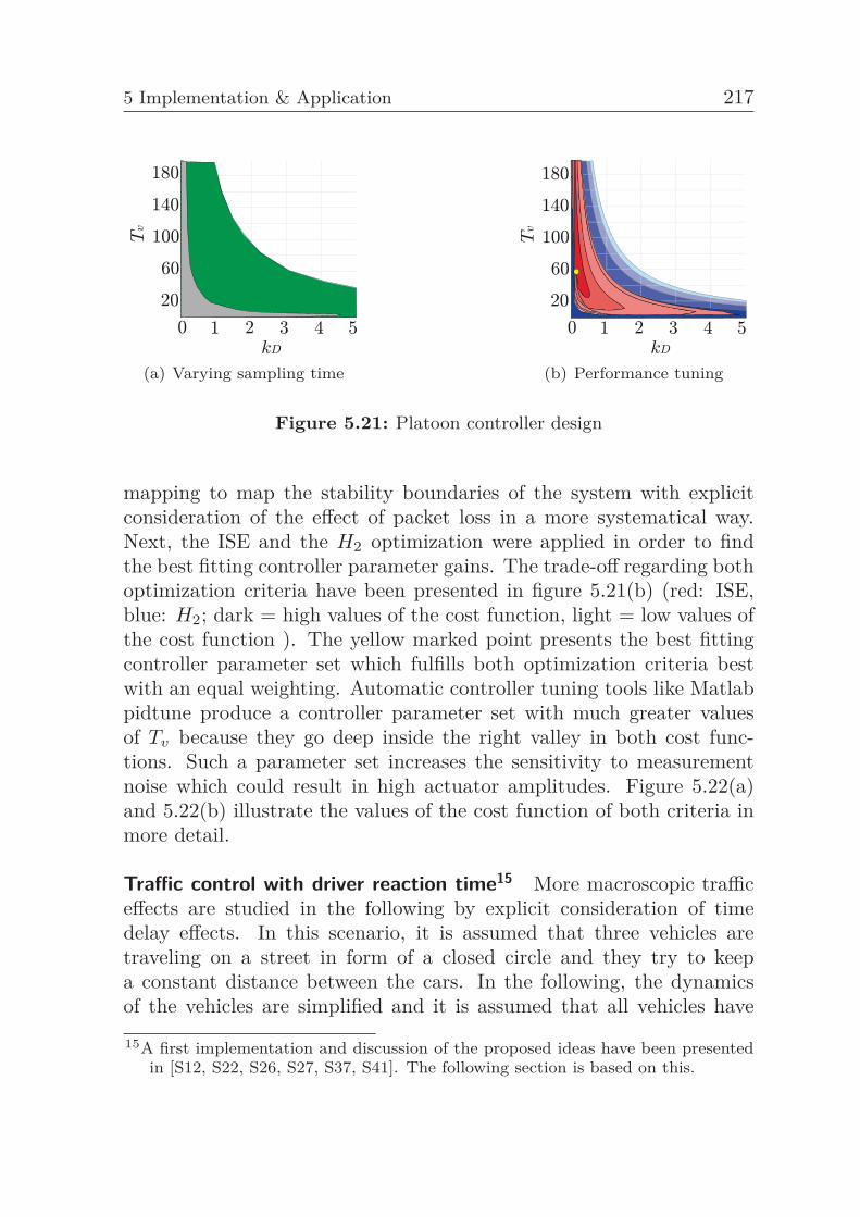
5 Implementation & Application 217
(a) Varying sampling time (b) Performance tuning
Figure 5.21: Platoon controller design
mapping to map the stability boundaries of the system with explicitconsideration of the effect of packet loss in a more systematical way.Next, the ISE and the H2 optimization were applied in order to findthe best fitting controller parameter gains. The trade-off regarding bothoptimization criteria have been presented in figure 5.21(b) (red: ISE,blue: H2; dark = high values of the cost function, light = low values ofthe cost function ). The yellow marked point presents the best fittingcontroller parameter set which fulfills both optimization criteria bestwith an equal weighting. Automatic controller tuning tools like Matlabpidtune produce a controller parameter set with much greater valuesof Tv because they go deep inside the right valley in both cost func-tions. Such a parameter set increases the sensitivity to measurementnoise which could result in high actuator amplitudes. Figure 5.22(a)and 5.22(b) illustrate the values of the cost function of both criteria inmore detail.
Traffic control with driver reaction time15 More macroscopic trafficeffects are studied in the following by explicit consideration of timedelay effects. In this scenario, it is assumed that three vehicles aretraveling on a street in form of a closed circle and they try to keepa constant distance between the cars. In the following, the dynamicsof the vehicles are simplified and it is assumed that all vehicles have
15A first implementation and discussion of the proposed ideas have been presentedin [S12, S22, S26, S27, S37, S41]. The following section is based on this.
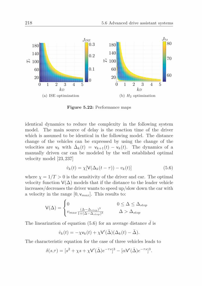
218 5.6 Advanced drive assistant systems
(a) ISE optimization (b) H2 optimization
Figure 5.22: Performance maps
identical dynamics to reduce the complexity in the following systemmodel. The main source of delay is the reaction time of the driverwhich is assumed to be identical in the following model. The distancechange of the vehicles can be expressed by using the change of thevelocities are vk with Δk(t) = vk+1(t) − vk(t). The dynamics of amanually driven car can be modeled by the well established optimalvelocity model [23,237]
vk(t) = χ[V(Δk(t− τ))− vk(t)] (5.6)
where χ = 1/T > 0 is the sensitivity of the driver and car. The optimalvelocity function V(Δ) models that if the distance to the leader vehicleincreases/decreases the driver wants to speed up/slow down the car witha velocity in the range [0, vmax]. This results to:
V(Δ) =
⎧⎨⎩0 0 ≤ Δ ≤ Δstop
vmax(Δ−Δstop)3
1+(Δ−Δstop)3 Δ > Δstop
The linearization of equation (5.6) for an average distance d is
vk(t) = −χvk(t) + χV′(Δ)(Δk(t)− Δ).
The characteristic equation for the case of three vehicles leads to
δ(s,τ) = [s2 + χs + χV′(Δ)e−τs]3 − [αV′(Δ)e−τs]3.
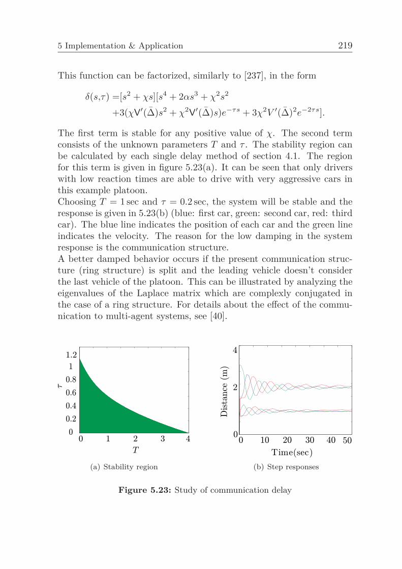
5 Implementation & Application 219
This function can be factorized, similarly to [237], in the form
δ(s,τ) =[s2 + χs][s4 + 2αs3 + χ2s2
+3(χV′(Δ)s2 + χ2V′(Δ)s)e−τs + 3χ2V ′(Δ)2e−2τs].
The first term is stable for any positive value of χ. The second termconsists of the unknown parameters T and τ . The stability region canbe calculated by each single delay method of section 4.1. The regionfor this term is given in figure 5.23(a). It can be seen that only driverswith low reaction times are able to drive with very aggressive cars inthis example platoon.Choosing T = 1 sec and τ = 0.2 sec, the system will be stable and theresponse is given in 5.23(b) (blue: first car, green: second car, red: thirdcar). The blue line indicates the position of each car and the green lineindicates the velocity. The reason for the low damping in the systemresponse is the communication structure.A better damped behavior occurs if the present communication struc-ture (ring structure) is split and the leading vehicle doesn’t considerthe last vehicle of the platoon. This can be illustrated by analyzing theeigenvalues of the Laplace matrix which are complexly conjugated inthe case of a ring structure. For details about the effect of the commu-nication to multi-agent systems, see [40].
(a) Stability region (b) Step responses
Figure 5.23: Study of communication delay
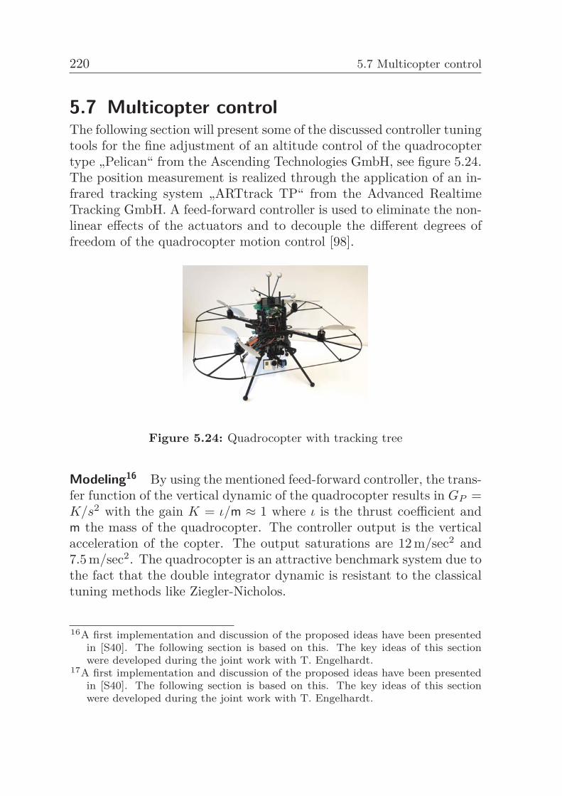
220 5.7 Multicopter control
5.7 Multicopter controlThe following section will present some of the discussed controller tuningtools for the fine adjustment of an altitude control of the quadrocoptertype „Pelican“ from the Ascending Technologies GmbH, see figure 5.24.The position measurement is realized through the application of an in-frared tracking system „ARTtrack TP“ from the Advanced RealtimeTracking GmbH. A feed-forward controller is used to eliminate the non-linear effects of the actuators and to decouple the different degrees offreedom of the quadrocopter motion control [98].
Figure 5.24: Quadrocopter with tracking tree
Modeling16 By using the mentioned feed-forward controller, the trans-fer function of the vertical dynamic of the quadrocopter results in GP =K/s2 with the gain K = ι/m ≈ 1 where ι is the thrust coefficient andm the mass of the quadrocopter. The controller output is the verticalacceleration of the copter. The output saturations are 12 m/sec2 and7.5 m/sec2. The quadrocopter is an attractive benchmark system due tothe fact that the double integrator dynamic is resistant to the classicaltuning methods like Ziegler-Nicholos.
16A first implementation and discussion of the proposed ideas have been presentedin [S40]. The following section is based on this. The key ideas of this sectionwere developed during the joint work with T. Engelhardt.
17A first implementation and discussion of the proposed ideas have been presentedin [S40]. The following section is based on this. The key ideas of this sectionwere developed during the joint work with T. Engelhardt.
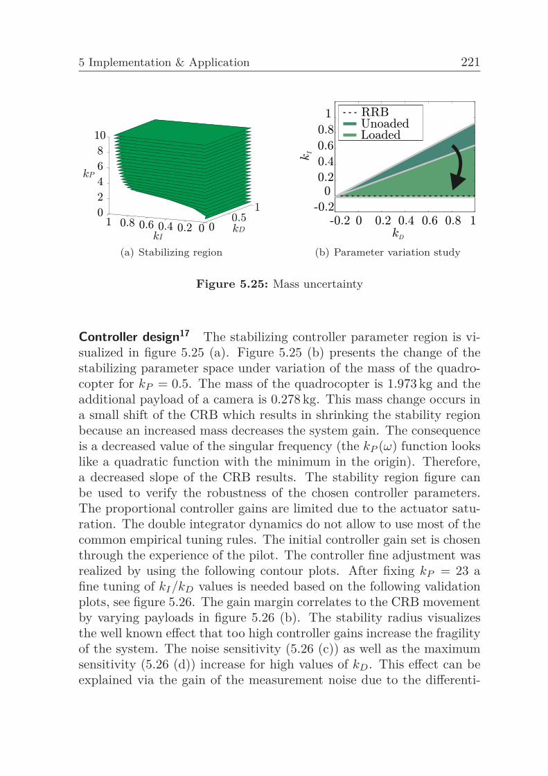
5 Implementation & Application 221
(a) Stabilizing region (b) Parameter variation study
Figure 5.25: Mass uncertainty
Controller design17 The stabilizing controller parameter region is vi-sualized in figure 5.25 (a). Figure 5.25 (b) presents the change of thestabilizing parameter space under variation of the mass of the quadro-copter for kP = 0.5. The mass of the quadrocopter is 1.973 kg and theadditional payload of a camera is 0.278 kg. This mass change occurs ina small shift of the CRB which results in shrinking the stability regionbecause an increased mass decreases the system gain. The consequenceis a decreased value of the singular frequency (the kP (ω) function lookslike a quadratic function with the minimum in the origin). Therefore,a decreased slope of the CRB results. The stability region figure canbe used to verify the robustness of the chosen controller parameters.The proportional controller gains are limited due to the actuator satu-ration. The double integrator dynamics do not allow to use most of thecommon empirical tuning rules. The initial controller gain set is chosenthrough the experience of the pilot. The controller fine adjustment wasrealized by using the following contour plots. After fixing kP = 23 afine tuning of kI/kD values is needed based on the following validationplots, see figure 5.26. The gain margin correlates to the CRB movementby varying payloads in figure 5.26 (b). The stability radius visualizesthe well known effect that too high controller gains increase the fragilityof the system. The noise sensitivity (5.26 (c)) as well as the maximumsensitivity (5.26 (d)) increase for high values of kD. This effect can beexplained via the gain of the measurement noise due to the differenti-
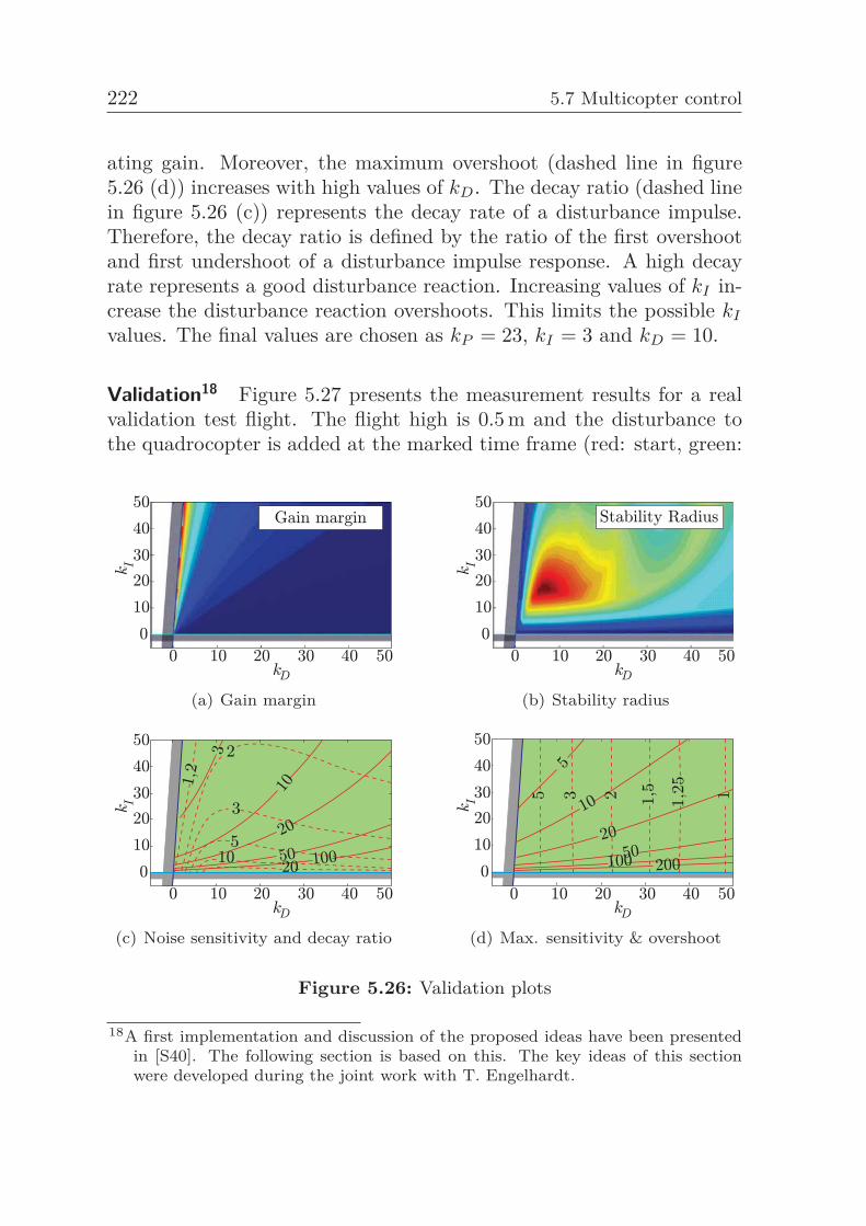
222 5.7 Multicopter control
ating gain. Moreover, the maximum overshoot (dashed line in figure5.26 (d)) increases with high values of kD. The decay ratio (dashed linein figure 5.26 (c)) represents the decay rate of a disturbance impulse.Therefore, the decay ratio is defined by the ratio of the first overshootand first undershoot of a disturbance impulse response. A high decayrate represents a good disturbance reaction. Increasing values of kI in-crease the disturbance reaction overshoots. This limits the possible kI
values. The final values are chosen as kP = 23, kI = 3 and kD = 10.
Validation18 Figure 5.27 presents the measurement results for a realvalidation test flight. The flight high is 0.5 m and the disturbance tothe quadrocopter is added at the marked time frame (red: start, green:
(a) Gain margin (b) Stability radius
(c) Noise sensitivity and decay ratio (d) Max. sensitivity & overshoot
Figure 5.26: Validation plots
18A first implementation and discussion of the proposed ideas have been presentedin [S40]. The following section is based on this. The key ideas of this sectionwere developed during the joint work with T. Engelhardt.
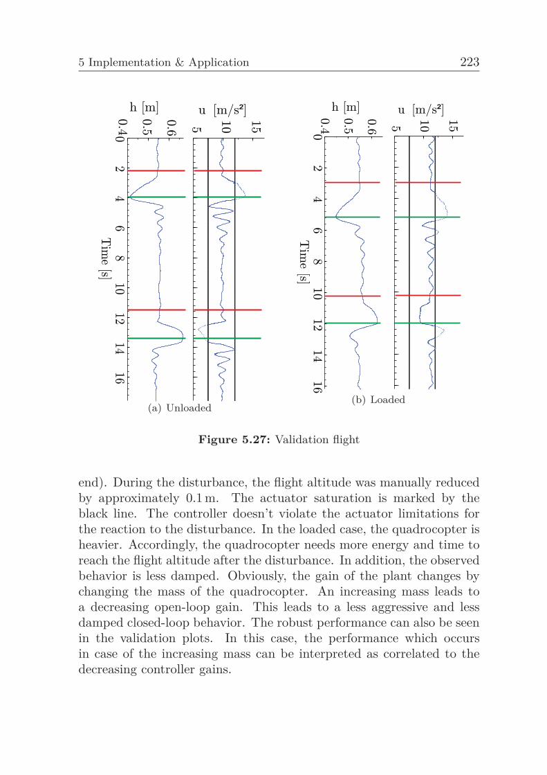
5 Implementation & Application 223
(a) Unloaded(b) Loaded
Figure 5.27: Validation flight
end). During the disturbance, the flight altitude was manually reducedby approximately 0.1 m. The actuator saturation is marked by theblack line. The controller doesn’t violate the actuator limitations forthe reaction to the disturbance. In the loaded case, the quadrocopter isheavier. Accordingly, the quadrocopter needs more energy and time toreach the flight altitude after the disturbance. In addition, the observedbehavior is less damped. Obviously, the gain of the plant changes bychanging the mass of the quadrocopter. An increasing mass leads toa decreasing open-loop gain. This leads to a less aggressive and lessdamped closed-loop behavior. The robust performance can also be seenin the validation plots. In this case, the performance which occursin case of the increasing mass can be interpreted as correlated to thedecreasing controller gains.
224
6 Conclusion and outlook
The present work focuses on the problem of robust controller synthesisand analysis based on stability region calculation methods. Today, thistheory is rarely used due to the large number of limitations regardingthe applicability. Accordingly, the present work offers a solution withinan unified formalism regarding the problem about stability region basedcontroller tuning. This enriches the practical usability of this hiddentheory.At first in section 2, a detailed comparison of different stability regioncalculation approaches including several expansions of the available ap-proaches were presented (e.g. PSA extension for mesh loop and statefeedback control structures). During this, it was detected that the sin-gular frequency calculation for the CRB becomes very complex for ad-vanced system structures. Therefore, a Lyapunov stability based calcu-lation approach was proposed which overcomes the problem of singularfrequency calculation. In addition, a generally applicable probabilisticstability region calculation method was introduced. Based on this, novelphenomena in the calculation and analysis of the stability region in thecontroller as well as the system parameter space were described and pre-cisely formulated for a wide class of systems. Thus, new fundamentalresults regarding the stabilizing controller parameter space calculationwere presented.At the beginning of section 3, which focuses on the robustness prob-lem, the analysis step was systematically studied. Moreover, severaldelay stability region approaches were discussed. It was presented thatall these approaches can be generalized to crossing frequency detectionmethods. Based on this, several expansions of the analysis step wereproposed. The classical analysis step was identified as a time consumingiterative method which is hard to apply for general plants. By usingclassical worst-case test sets the robust controller design method wassimplified to a one step procedure with explicit consideration of param-eter uncertainties. Moreover, the stability movement based approachwas introduced. Therefore, the exact robust stabilizing parameter space
6 Conclusion and outlook 225
was analytically calculated for delay-free plants with interval and affineparameter uncertainties. For more advanced systems as well as un-certainty classes, several parameter space approximation methods weredemonstrated. During the calculation there was a trade-off betweencomputational effort and conservatism of the resulting robust stabiliz-ing parameter space for all the methods detected.Thereafter in section 4, it was shown that it is hard to manually findthe best fitting controller set inside the stability region without usingany additional performance tuning methods. Therefore, several stabil-ity region based controller tuning methods were introduced. Most ofthese methods are focusing on controller parameter tuning of time de-lay systems. A variety of methods was illustrated to make an efficientcontroller tuning possible. This includes the presentation of differentperformance maps as well as a study regarding finding a suitable ini-tial set of controller gains for the fine tuning. Moreover, an efficientcompletely automatic controller optimization method based on the sta-bilizing parameter space was presented. All these methods will increasethe usability of the stability region based controller tuning methodsstrongly.All the developed methods are available in the open source Delay SystemRobust Control (DSRC) toolbox for Matlab which can be accessed viathe website (http://www.irt.rwth-aachen.de/pidrobust). In sec-tion 5, some of the developed results were applied to several practi-cal examples from different fields of applications like process control,combustion, aviation and automotive. It was in detail described howthe robust controller tuning is used in these applications. This offersa transparent insight how the developed methods can enrich the con-troller tuning procedure in daily life. All this helps in order to bringthe new theoretical developments into industrial practice.In the future, it would be interesting to expand the Lyapunov basedstability region calculation approach to additional system classes. Also,the development of additionally full automatic stability region basedcontroller tuning methods look promising. Last but not least the appli-cation of the parameter space based controller tuning methods to severalchallenging real life controller tuning problems is desirable. This is atask with high priority, especially in the case of an approach which isstill unknown in industrial praxis.
226
Bibliography
[1] P. R. Acioli and G. Barros. Loop-shaping PI controller redesignusing least-squares model-matching. Proc. of 8th InternationalSymposium on Dynamics and Control of Process Systems, 2007.
[2] J. Ackermann. Parameter space design of robust control sys-tems. IEEE Transactions on Automatic Control, 25(12):1058–1072, 1980.
[3] J. Ackermann. Does it suffice to check a subset of multilinear pa-rameters in robustness analysis. IEEE Transactions on AutomaticControl, 37:487–488, 1992.
[4] J. Ackermann, P. Blue, T. Bünte, L. Güvenc, D. Kaesbauer,M. Kordt, and D. Odenthal. Robust control: The parameter spaceapproach. Springer, 2002.
[5] J. Ackermann and C. Hollot. On extreme-point results for time-delay systems. Proc. of American Control Conference, 1990.
[6] J. Ackermann, D. Kaesbauer, and N. Bajcinca. Discrete-timerobust PID and three-term control. Proc. of 15th IFAC WorldCongress, 2002.
[7] J. Adamy. Nichtlineare Systeme und Regelungen. Springer, 2014.
[8] P. Airikka. Predictive PID controller for integrating processeswith long dead times. IEEE ASSP Magazine, 3:475–480, 2014.
[9] P. Albertos and A. Sala. Advanced textbooks in control and signalprocessing. Springer, 2003.
[10] J. Anagnost, C. Desoer, and R. Minichelli. Generalized nyquisttest for robust stability: frequency domain generalizations ofkharitonovs theorem. Robustness in Identification and Control,pages 79–96, 1989.
Bibliography 227
[11] B. Anderson, E. Jury, and M. Mansour. On robust hurwitz poly-nomials. IEEE Transactions on Automatic Control, 32(10):909–913, 1987.
[12] B. D. O. Anderson and J. B. Moore. Optimal control - linearquadratic methods. Prentice-Hall, 1989.
[13] K. H. Ang, G. Chong, and Y. Li. PID control system analysis,design and technology. IEEE Transactions on Control SystemsTechnology, 13(4):559–576, July 2005.
[14] P. K. Anochin. Beiträge zur allgemeinen Theorie des funktionellenSystems. VEB Gustav Fischer Verlag Jena, 1978.
[15] P. Apkarian and D. Noll. Nonsmooth H∞ synthesis. IEEE Trans-actions on Automatic Control, 51(1):71–86, 2006.
[16] R. Ash and G. Ash. Numerical computation of root loci usingthe newton-raphson technique. IEEE Transactions on AutomaticControl, 13(5):576–582, 1968.
[17] F. M. Asl and A. G. Ulsoy. Analytical solution of a system ofhomogeneous delay differential equations via the lambert function.Technical report, University of Michigan, 2000.
[18] K. J. Aström. Control system design. Technical report, Universityof California, 2002.
[19] K. J. Aström and K. Furuta. Swinging up a pendulum by energycontrol. Automatica, 36(2):287–295, 2000.
[20] K. J. Aström and T. Hägglund. PID controllers: Theory, designand tuning. Instrument Society of America, Research TrianglePark, NC, 1995.
[21] K. J. Aström, T. Hägglund, and H. Panagopoulos. Design ofPI controllers based on non-convex optimization. Automatica,34(5):585–601, 1998.
[22] K. J. Aström and P. R. Kumar. Survey control: A perspective.Automatica, 50(1):3–43, 2014.
[23] F. M. Atay. Complex Time-Delay Systems: Theory and Applica-tions. Springer, 2010.
228 Bibliography
[24] P. Atkinson and V. S. Dalvi. An improved algorithm for theautomatic determination of root loci by digital computer. Radioand Electronic Engineer, 41(8):365–371, 1971.
[25] S. Avanessov and U. Nurges. Stability domain approximation forthe robust PID controller parameters by reflection segments ap-proach. Proc. of IEEE Chinese Control and Decision Conference,pages 2004–2009, 2013.
[26] S. Avanessov and U. Nurges. Reflection segments based ro-bust PID controller solution for benchmark problem. Proc. ofIEEE 22nd Mediterranean Conference on Control and Automa-tion, 2014.
[27] N. Bajcinca. Computation of stable regions in PID parameterspace for time-delay systems. Proc. of 5th IFAC Workshop onTime-Delay Systems, 2004.
[28] N. Bajcinca. Discrete-time robust design for PID and three-termcontrol based on decoupling at singular frequencies. Journal ofTransactions on Automatic Control, (10):1–7, 2004.
[29] N. Bajcinca. Design of robust PID controllers using decouplingat singular frequencies. Automatica, 42(11):1943–1949, 2006.
[30] N. Bajcinca and T. Hulin. RobSin: A New Tool for Robust Designof PID and Three-Term Controllers based on Singular Frequen-cies. Proc. of CACSD/ISIC/CCA, 2004.
[31] N. Bajcinca and T. Hulin. Menge aller robust stabilisieren-den PID-Regler: Methodik und software (Teil I). at - Automa-tisierungstechnik, 53(11):556–564, 2005.
[32] G. Baker. PID tuning of plants with time delay using root locus.Master’s thesis, San Jose State University, 2011.
[33] B. Barmigh, C. Hollot, F. Kraus, and R. Tempo. Extreme pointresults for robust stabilization of interval plants with first ordercompensators. IEEE Transactions on Automatic Control, 37:707–712, 1992.
[34] B. R. Barmish. New tools for robustness of linear systems.Macmillan, 1993.
Bibliography 229
[35] B. R. Barmish and R. Tempo. The robust root locus. Proc. ofthe 27th IEEE Conference on Decision and Control, 1988.
[36] A. Bartlett, C. Hollot, and H. Lin. Root locations of an entirepolytope of polynomials: It suffices to check the edges. Mathe-matics of Control, Signals and Systems, 1(1):61–71, 1988.
[37] N. Bayhan and M. T. Söylemez. Fast calculation of all stabilizinggains for discrete-time systems. Journal of electrical & electronicsengineering, 6:19–26, 2006.
[38] T. Becker. Numerische Berechnung von Wurzelortskurven überdie Analogie zu ebenen Potentialströmungen. at - Automa-tisierungstechnik, 36(5):179–183, 1988.
[39] R. Bellman and K. L. Cooke. Differential-difference equations.Academic Press, 1963.
[40] A. Bemporad, M. Heemels, and M. Johansson. Networked con-trol systems, lecture notes in control and information sciences.Springer, 2011.
[41] M. M. Berry. A variable-step double-integration multi-step in-tegrator. Dissertation, Virginia Polytechnic Institute and StateUniversity, 2004.
[42] D. Bertsekas. Nonlinear programming. Athena Scientific, 2. edi-tion, 1999.
[43] V. Besson and A. T. Shenton. Interactive control system designby a mixed H∞-parameter space method. IEEE Transactions onAutomatic Control, 42(7):946–955, 1997.
[44] S. P. Bhattacharyya, H. Chapellat, and L. H. Keel. Robust con-trol: The parametric approach. Prentice Hall, 1995.
[45] S. P. Bhattacharyya, A. Datta, and L. H. Keel. Linear controltheory: Structure, robustness and optimization. CRC Press, 2012.
[46] S. P. Bhattacharyya and L. H. Keel. Control of uncertain dynamicsystems. CRC Press, 1991.
230 Bibliography
[47] S. Bialas. A necessary and sufficient condition for the stability ofconvex combinations of stable polynomials or matrices. Bulletinof the Polish Academy of Sciences, pages 473–480, 1985.
[48] W. L. Bialkowski. Control of the pulp and paper making process.W. S. Levine, The Control Handbook - CRC/IEEE Press, pages1219–1242, 1996.
[49] J. T. Bingham and L. H. Ting. Stability radius as a methodfor comparing the dynamics of neuromechanical systems. NeuralSystems and Rehabilitation Egineering, 2013.
[50] A. Björck. Numerical methods for least squares problems. SIAM,1996.
[51] T. Bünte. Beiträge zur robusten Lenkregelung von Personenkraft-wagen. Dissertation, RWTH Aachen, 1998.
[52] T. Bünte. Mapping of nyquist/popov theta-stability margins intoparameter space. Proc. of 3rd IFAC Symposium on Robust ControlDesign, 2000.
[53] T. Bünte. Die Anwendung des Parameterraumverfahrens auf Ort-skurvenkriterien. at - Automatisierungstechnik, 49(12):547–556,2001.
[54] H. W. Bode. Network analysis & feedback amplifier design. D.Van Nostrand Company, 1945.
[55] O. R. Bosede, F. S. Emmanue, and O. J. Temitayo. On somenumerical methods for solving initial value problems in ordinarydifferential equations. Technical report, Ekiti State University,Nigeria and Afe Babalola University, 2012.
[56] O. Bosgra and H. Kwakernaak. Design methods for control sys-tems. Dutch Institute of Systems and Control, 2000.
[57] S. Boyd, L. ElGhaoui, E. Feron, and V. Balakrishnan. Linearmatrix inequalities in system and control theory. SIAM Studiesin Applied Mathematics, 1994.
[58] S. Boyd and L. Vandenberghe. Convex Optimization. CambridgeUniversity Press, 2004.
Bibliography 231
[59] M. Bozorg. Linear systems with a polynomial uncertainty struc-ture: Stability margins & control. Journal of Systems and ControlEngineering, 220:53–62, 2006.
[60] M. Bozorg. Robust performance margins and robust controllerdesign for systems with uncertain parameters. Journal of Systemsand Control Engineering, 6:511–521, 2008.
[61] M. Bozorg, H. Sherali, E. Davison, and J. Desai. Computationof parameters stability margins using polynomial programmingtechniques. International Journal of Control, 79:739–751, 2006.
[62] J. W. Brewer. Kronecker products and matrix calculus in systemtheory. IEEE Trans. Circuits Syst., 25:772–781, 1978.
[63] N. Bruinsma and M. Steinbuch. A fast algorithm to computethe H∞ norm of a transfer function matrix. Systems and ControlLetters, 14:287–293, 1990.
[64] W. E. Brumley. On the asymptotic behavior of solutions of dif-ferential difference equations of neutral type. Technical report,Colorado State University, 1968.
[65] J. V. Burke, A. S. Lewis, and M. L. Overton. Robust stabilityand a criss-cross algorithm for pseudospectra. IMA Journal ofNumerical Analysis, 23:359–375, 2003.
[66] R. H. Byrd, E. H. Mary, and J. N. An interior point algorithm forlarge-scale nonlinear programming. SIAM Journal on Optimiza-tion, 9(4):877–900, 1999.
[67] G. Calafiore, F. Dabbene, and R. Tempo. Randomized algorithmsfor probabilistic robustness with real and complex structured un-certainty. IEEE Transactions on Automatic Control, 45:2218–2235, 2000.
[68] E. F. Camacho and A. C. Bordons. Model predictive control.Springer, 2007.
[69] M. Chamanbaz, F. Dabbene, D. Peaucelle, and R. Tempo. R-romuloc: A unified tool for randomized and robust multiobjectivecontrol. Proc. of IFAC Conference on Robust Control Design,2015.
232 Bibliography
[70] C. Chang. An analytical method for obtaining the root locus withposititve and negative gain. IEEE Transactions on AutomaticControl, 10(1):92–94, 1964.
[71] C. Chen and C. Hsu. The determination of root loci using Routh’salgorithm. Journal of the Franklin Institute, 281(2):114–121, 1966.
[72] J. Chen and S. I. Niculescu. Robust stability of quasipolynomi-als: vertex-type tests and extensions. Proc. of American ControlConference, 2004.
[73] Y. Q. Chen and K. L. Moore. Analytical stability bound fordelayed second-order systems with repeating poles using Lambertfunction W. Technical report, Utah State University, 2000.
[74] M. Chilali and P. Gahinet. H∞ design with pole placement con-straints: An LMI approach. IEEE Transactions on AutomaticControl, 41(3):358–366, 1996.
[75] U. Christen. Engineering Aspects of H∞ Control. Dissertation,ETH Zürich, 1996.
[76] P. Cominos and N. Munro. PID controllers: Recent tuning meth-ods and design to specification. Technical Report 1, IEE Proceed-ings, 2002.
[77] K. L. Cooke and P. van den Driessche. On zeros of some tran-scendental equations. Funkcialaj Ekvacioj, 29:77–90, 1986.
[78] D. A. Cox, J. Little, and D. O’Shea. Using algebraic geometry(graduate texts in mathematics). Springer, 2005.
[79] S. Dasgupta. Kharitonovs theorem, revisited. Systems and Con-trol Letters, 11:381–384, 1988.
[80] R. Datko. A procedure for determination of the exponential stabil-ity of certain differential-difference equations. Quart. Appl. Math.,36:279–292, 1978.
[81] A. Datta, M. Ho, and S. Bhattacharyya. Structure and synthesisof PID controllers. Advances in Industrial Control, Springer, 2010.
Bibliography 233
[82] A. Datta, M. T. Ho, and S. P. Bhattacharyya. Advances in indus-trial control: structures and synthesis of PID controller. Springer,1999.
[83] J. E. Dennis and R. B. Schnabel. Numerical methods for uncon-strained optimization and nonlinear equations. SIAM, Philadel-phia, 1996.
[84] P. V. der Kloet and F. L. Neerhoff. On eigenvalues and polesfor second order linear time varying systems. Proc. of the IEEEWorkshop on Nonlinear Dynamics of Electronic Systems, pages300–305, 1997.
[85] P. V. der Kloet and F. L. Neerhoff. The characteristic equationfor time varying models of nonlinear dynamic systems. Proc. ofEuropean Conference on Circuit Theory and Design, 2001.
[86] P. V. der Kloet and F. L. Neerhoff. Dynamic eigenvalues forscalar linear time varying systems. Proc. of 15th Int. Symp. onMathematical Theory of Net. and Sys., 2002.
[87] L. Desborough and R. Miller. Increasing customer value of in-dustrial control performance monitoring - Honeywell’s experience.Proc. of Sixth International Conference on Chemical Process Con-trol, 98:169–189, 2002.
[88] P. Deuflhard and A. Hohmann. Numerical analysis in modernscientific computing. Springer, 2003.
[89] T. E. Djaferis. Robust control design: A polynomial approach.Kluwer Academic Publishers, 1995.
[90] D. J. Doda. The digital computer makes root locus easy. ControlEngineering, 5:102–106, 1958.
[91] R. C. Dorf and R. H. Bishop. Modern control systems. PrenticeHall, Upper Saddle River and NJ, 12. edition, 2010.
[92] J. C. Doyle, K. Glover, P. P. Khargonekar, and B. A. Francis.State-space solutions to standard H2 and H∞ control problems.IEEE Transactions on Automatic Control, 4(4):831–847, 1989.
234 Bibliography
[93] G. R. Duan. Analysis and Design of Descriptor Linear Systems.Springer, 2010.
[94] W. Duffek. Astweise Berechnung von Wurzelortskurven. DeutscheForschungs- und Versuchsanstalt für Luft-und Raumfahrt, Ober-pfaffenhofen, 1971.
[95] C. Ebenbauer and F. Allgöwer. Stability analysis for time-delaysystems using rekasius substitution and sum of squares. Proc. ofIEEE Conf. Decision Control, 45:5376–5381, 2006.
[96] T. Emami, T. Lee, and J. M. Watkins. Stability Regions in theParameter Space for a Unified PID Controller. Proc. of AmericanControl Conference, 2010.
[97] D. B. Ender. Process control performance: not as good as youthink. Control Engineering Practice, 40:180–186, 1993.
[98] T. Engelhardt and D. Abel. MPC Trajectory Generation for aFlatness based Control of a Quadrotor Camera Helicopter. Proc.of European Control Conference, 2016.
[99] Eurotransplant. Eurotransplant statistic.http://www.eurotransplant.org, visited on 03.12.2014.
[100] W. R. Evans. Graphical analysis of control systems. Transactionsof the American Institute of Electrical Engineers, 67(1):547–551,1948.
[101] W. R. Evans. Control system synthesis by root locus method.Transactions of the American Institute of Electrical Engineers,69(1):66–69, 1950.
[102] G. P. Falconí. Robust semi-automatic design of PID controllersfor systems with time delay. Studienarbeit, Technische UniversitätMünchen, 2012.
[103] B. Fang and J. Kong. New approach to the realization of PIDcontroller parameter stable regions. Proc. of IEEE InternationalConference on Computer Science and Automation Engineering,2:627–631, 2011.
Bibliography 235
[104] S. Farhati, B. H. A. Naoui, and M. Abdelkrim. H∞ Loop ShapingControl of time delay systems. Proc. of International Conferenceon Communications, Computing and Control Applications, 2011.
[105] O. Föllinger. Nichtlineare Regelungen II. De Gruyter Oldenbourg,1993.
[106] B. A. Francis. A Course in H∞ Control Theory. Springer, 1987.
[107] R. W. Freund and R. H. W. Hoppe. Numerische Mathematik 1.Springer, 10. edition, 2007.
[108] E. Fridman. Tutorial on Lyapunov-based Methods for Time-Delay Systems. European Journal of Control, 20:271–283, 2014.
[109] E. Fridman. Introduction to Time-Delay Systems - Analysis andControl. Birkhäuser, 2014.
[110] M. Fu, A. Olbrot, and M. Polis. Robust stability for time-delaysystems: The edge theorem and graphical tests. IEEE Transac-tions on Automatic Control, pages 813–820, 1989.
[111] P. Gahinet and P. Apkarian. A linear matrix inequality approachto H∞ control. International Journal of Robust and NonlinearControl, 4:421–448, 1994.
[112] P. Gahinet, P. Apkarian, and M. Chilali. Affine parameter-dependent Lyapunov functions and real parametric uncertainty.IEEE Transactions on Automatic Control, 41(3):436 – 442, 1996.
[113] P. Gahinet, P. Apkarian, and M. Chilali. Affine parameter-dependent lyapunov functions and real parametric uncertainty.IEEE Transactions on Automatic Control, 41(3):436–442, 1996.
[114] O. Garpinger, T. Hägglund, and K. J. Aström. Criteria and trade-offs in PID design. Proc. of IFAC Conference on Advances in PIDControl, pages 28–30, 2012.
[115] M. Ge, M. S. Chiu, and Q. G. Wang. Robust PID controller designvia LMI approach. Journal of Process Control, 12:3–13, 2003.
[116] H. P. Geering. Lecture notes: Regelungstechnik II. Institut fürMess- und Regeltechnik, ETH-Zürich, 2. edition, 2004.
236 Bibliography
[117] H. P. Geering. Lecture notes: Robuste regelung. Institut für Mess-und Regeltechnik, ETH-Zürich, 4. edition, 2007.
[118] H. P. Geering and A. Roduner. Entwurf robuster Regler mit H∞-Methode. Bulletin SEV/VSE, 3:55–58, 1999.
[119] J. Gerry and P. Hansen. Choosing the right controller. Chem.Eng., pages 65–68, May 25 1987.
[120] G. T. Gilbert. Positive definite matrices and Sylvester’s criterion.The American Mathematical Monthly, 98:44–46, 1991.
[121] G. H. Golub and C. V. Loan. Matrix Computations. The JohnsHopkins University Press, 4th edition, 2013.
[122] C. Grimholt and S. Skogestad. Optimal PI-control and verificationof the SIMC tuning rule. Proc. of IFAC conference on Advancesin PID control, 2012.
[123] G. Grübel and L. Schmieder. Die Eigenschaften verallgemein-erter Wurzelortskurven. Deutsche Versuchsanstalt für Luft- undRaumfahrt Zentralstelle, München, 1967.
[124] E. N. Gryazina and B. T. Polyak. Stability regions in the param-eter space: D-decomposition revisited. Automatica, 42(1):13–26,2006.
[125] E. N. Gryazina, B. T. Polyak, and A. A. Tremba. D-decompositiontechnique state-of-the-art. Automation and Remote Control,69(12):1991–2026, 2008.
[126] K. Gu, V. L. Kharitonov, and J. Chen. Stability of time-delaysystems. Birkhäuser, 2003.
[127] K. Gu and M. Naghnaeian. Stability crossing set for systems withthree delays. IEEE Transactions on Automatic Control, 56(1):11–26, 2011.
[128] K. Gu and S. I. Niculescu. Survey on recent results in the stabilityand control of time-delay systems. Journal of Dynamic Systems,Measurement and Control, 125:158–165, 2003.
Bibliography 237
[129] K. Gu, S. I. Niculescu, and J. Chen. On stability crossing curvesfor general systems with two delays. Journal of MathematicalAnalysis and Applications, 311:231–253, 2005.
[130] A. N. Guendes, H. Oezbay, and A. B. Oezgueler. PID controllersynthesis for a class of unstable MIMO plants with I/O delays.Automatica, 43(1):135–142, 2007.
[131] S. Gumussoy and W. Michiels. Root locus for siso dead-timesystems: A continuation based approach. Automatica, 48(3):480–489, 2012.
[132] M. A. Gutierrez de Anda. A study of the time varying eigenvaluesand their application in circuit design. Dissertation, Electrical En-gineering, Mathematics and Computer Science, Delft Universityof Technology, 2003.
[133] S. Gutman. Lecture notes in control and information science.Springer-Verlag, Berlin, 1990.
[134] L. Güvenç and J. Ackermann. Links between the parameter spaceand frequency domain methods of robust control. InternationalJournal of Robust and Nonlinear Control, 11:1435–1453, 2001.
[135] M. Habigt, M. Ketelhut, J. Gesenhues, F. Schrödel, M. Hein, T. S.Rhode, R. Rossaint, and D. Abel. Comparison of Novel Physio-logical Load-Adaptive Control Strategies for Ventricular AssistDevices. Biomedizinische Technik/Biomedical Engineering, 2016(under review).
[136] J. K. Hale and W. Huang. Global geometry of the stable re-gions for two delay differential equations. Journal of MathematicalAnalysis and Applications, 178:344–362, 1993.
[137] P. D. Hansen. Parametric robustness. In Proc. of IFAC Confer-ence on Advances in PID Control, 2012.
[138] V. Hanta and A. Procházka. Rational approximation of timedelay. Technical report, Institute of Chemical Technology, Prague,2009.
[139] F. Haugen. PID-control. Tapir Academic Press, 2004.
238 Bibliography
[140] S. A. He and I. K. Fong. Stability and performance of first-orderlinear time-delay feedback systems: An eigenvalue approach.Technical report, National Taiwan University, 2011.
[141] D. Henrion. Optimization on linear matrix inequalities for polyno-mial systems control. International Summer School of AutomaticControl (free web access), 2014.
[142] D. Henrion and O. Bachelier. Low-order robust controller designfor interval plants. International Journal of Control, 74(1):1–9,2001.
[143] G. Herjólfsson, A. S. Hauksdóttir, and S. P. Sigurðsson. A two-stage optimization PID algorythm. Technical report, Universityof Iceland, 2012.
[144] B. Higgins. Letter from Dr. Higgins To Mr. Nicholson. Journalof Natural Philosophy and Chemical Arts, 1:1, 1802.
[145] M. T. Ho. Synthesis of H∞ PID controllers: A parametric ap-proach. Automatica, 39(6):1069–1075, 2003.
[146] N. Hohenbichler. All stabilizing PID controllers for time delaysystems. Automatica, 45:2678–2684, 2009.
[147] N. Hohenbichler. Robuster Reglerentwurf auf Grundlage derMenge aller stabilisierenden PID-Regler. Dissertation, RWTHAachen, 2009.
[148] N. Hohenbichler and D. Abel. Robust PID-controller design meet-ing pole location and gain/phase margin requirements for timedelay systems. at - Automatisierungstechnik, 54:495–501, 2006.
[149] N. Hohenbichler and D. Abel. Calculating all KP admitting sta-bility of a PID control loop. Proceedings of the 17th IFAC WorldCongress, 17:5802–5807, 2008.
[150] N. Hohenbichler and J. Ackermann. Computing stable regions inparameter spaces for a class of quasipolynomials. Proc. of IFACWorkshop on Time Delay Systems, 2003.
Bibliography 239
[151] A. L. Holene. Performance and Robustness of Smith PredictorControl and Comparison with PID Control. PhD thesis, NTNUTrondheim, 2013.
[152] O. Holtz. Hermite-Biehler, Routh-Hurwitz and total positivity.Linear Algebra and its Applications, 372:105–110, 2003.
[153] M. Hoppe, F. Schrödel, M. Reiter, J. Maschuw, H. Arenbeck, andD. Abel. Improvement of practical orientation in teaching by in-troduction of an innovative laboratory and competition. Proc. of.10th IFAC Symposium on Advances in Control Education, 2013.
[154] C. S. Hsu and S. J. Bhatt. Stability charts for second-order dy-namical systems with time lag. Journal of Applied Mechanics,33(1):119–124, 1966.
[155] M. Huba. Setpoint versus disturbance responses of the IPDTplant. Proc. of IFAC conference on advances in PID control, 2012.
[156] T. Hulin. Software-Werkzeug zur Auslegung von robusten PID-Reglern. Master’s thesis, Technische Universität München, 2003.
[157] T. Hulin, A. Albu-Schäffer, and G. Hirzinger. Passivity and sta-bility boundaries for haptic systems with time delay. IEEE Trans-actions on Control Systems Technology, 2014.
[158] A. Hurwitz. Über die Bedingungen, unter welchen eine Gleichungnur Wurzeln mit negativen reellen Teilen besitzt. MathematischeAnnalen, 46(2):273–284, 1895.
[159] C. Hwang and J. H. Hwang. On stabilization of first-order plusdead-time unstable processes using PID controllers. Proc. of Eu-ropean Control Conference, 2003.
[160] T. Insperger and G. Stepan. Semi-discretization for time-delaysystems: Stability and engineering applications. Springer, 2011.
[161] G. G. J. Chen and C. N. Nett. A new method for computing delaymargins for stability of linear delay systems. System and ControlLetters, 26:107–117, 1995.
240 Bibliography
[162] N. K. Jain and K. Singhal. Computing system roots and theirsensitivities. IEE Proceedings G Electronic Circuits and Systems,130(5):178–184, 1983.
[163] V. Jain and B. K. Lande. Computation of the state transition ma-trix for general linear time varying systems. International Journalof Engineering Research And Technology, 1, 2012.
[164] M. Jalili-Khareejoo and B. N. Araabi. The Schur stability viathe Hurwitz stability analysis using a biquadratic transformation.Automatica, 41(1):173–176, 2005.
[165] R. Jeltsch and M. Mansour. Stability theory: Hurwitz Cente-nary Conference. International Series of Numerical Mathematics,Birkhäuser, pages 67–69, 1996.
[166] E. I. Jury and J. Blanchard. A stability test for linear discretesystems in table form. IRE Proceedings, 14, 49(12):1947–1948,1961.
[167] D. Kaesbauer. Solving nonlinear parametric mapping equations.Proc. of 3rd IFAC Symposium on Robust Control Design, 2000.
[168] D. Kaesbauer and J. Ackermann. The distance from stability orγ-stability boundaries. Proc. of 11th IFAC World Congress, 1990.
[169] E. W. Kamen. The poles and zeros of a linear time-varying system.Linear Algebra and its Applications, 98:263–289, 1988.
[170] L. H. Keel, J. I. Rego, and S. P. Bhattacharya. A new approachto digital PID controller design. Transactions on Automation andControl, 48(4):687 – 692, 2003.
[171] H. K. Khalil. Nonlinear control. Prentice Hall, 2014.
[172] V. L. Kharitonov. Time-Delay Systems: Lyapunov Functionalsand Matrices. Birkhäuser, 2013.
[173] F. Kiani and M. Bozorg. Design of Digital PID Controllers Usingthe Parameter Space Approach. International Journal of Control,79(6):624–629, 2006.
Bibliography 241
[174] F. Kianzi and M. Bozorg. Design of digital PID controllers usingthe parameter space approach. International Journal of Control,2006.
[175] T. Kimura. On Dormand-Prince method. Technical report, JapanMalaysia Technical Institute, Senior Volunteer of Japan Interna-tional Cooperative Association, 2009.
[176] Z. Klagsbrunn and Y. Wallach. On computer implementation ofanalytic root-locus plotting. IEEE Transactions on AutomaticControl, 13(6):744–745, 1968.
[177] M. Kordt and J. Ackermann. Robust synergetic design of struc-tural dynamic engine out controllers in parameter space. Journalof Guidance, Control and Dynamics, 24(2):305–314, 2001.
[178] W. Krajewski and U. Viaro. Root-locus invariance exploiting al-ternative arrival and departure points. IEEE Control Systems,27(1):36–43, 2007.
[179] A. M. Krall and R. Fornaro. Root locus diagrams by digital com-puter. National Aeronautics and Space Administration, 1966.
[180] A. M. Krall and R. Fornaro. An algorithm for generating rootlocus diagrams. Commun. ACM, 10(3):186–188, 1967.
[181] F. Kraus, M. Mansour, and B. Anderson. Robust stability ofpolynomials with multilinear parameter dependence. Robustnessin Identification and Control, pages 263–280, 1989.
[182] F. J. Kraus, M. Mansour, and M. Sebek. Hurwitz matrix for poly-nomial matrices. International Series of Numerical Mathematics,Birkhäuser, 121, 1996.
[183] D. Kressner and B. Vandereycken. Subspace methods for com-puting the pseudospectral abscissa and the stability radius. SIAMJournal on Matrix Analysis and Applications, 35:292–313, 2014.
[184] V. Krishnan. Semi-analytic approach to root locus. IEEE Trans-actions on Automatic Control, 11(1):102–108, 1966.
[185] S. D. Kumar. Some important notions of Gröbner basis and Buch-berger’s algorithm. ASM, 2006.
242 Bibliography
[186] J. B. Lasserre. Characterizing polynomials with roots in a semial-gebraic set. IEEE Transactions on Automatic Control, 49(5):727–731, 2004.
[187] G. Leena, K. Dutta, and G. Ray. A set of stabilizing PD con-trollers for Multi-Input-Multi-Output systems. Proc. of Interna-tional Conference on Electrical and Computer Engineering, 2008.
[188] M. Lelić and Z. Gajić. A reference guide to PID controllers inthe nineties. Proc. of Workshop on Digital Control: Past, Presentand Future of PID Control, pages 19–30, 2000.
[189] J. Li and P. Li. Stability regions analysis of PID controllers fortime-delay systems. Proc. of the Sixth IEEE World Congress onIntelligent Control and Automation, 1:2219–2223, 2006.
[190] J. Louisell. A matrix method for determining the imaginary axiseigenvalues of a delay system. IEEE Transactions on AutomaticControl, 46(12):2008–2012, 2001.
[191] J. Lunze. Regelungstechnik 1 - Systemtheoretische Grundlagen,Analyse und Entwurf einschleifiger Regelungen. Springer, 8. edi-tion, 2010.
[192] J. Lunze. Regelungstechnik 2 - Mehrgrößensysteme, DigitaleRegelung. Springer, 6. edition, 2010.
[193] U. Mackenroth. Robust control systems: Theory and case studies.Springer, 2004.
[194] M. S. Mahmoud. Robust control and filtering for time-delay sys-tems. CRC Press, 2000.
[195] S. Malan, M. Milanese, and M. Taragna. Robust analysis anddesign of control systems using interval arithmetic. Automatica,33(7):1363–1372, 1997.
[196] B. P. Mann and B. R. Patel. Stability of delay equations writtenas state space models. Journal of Vibration and Control, 16:1067–1085, 2010.
Bibliography 243
[197] M. Mansour. On robust stability of time-varying linear systems.International Series of Numerical Mathematics, Birkhäuser, 121,1996.
[198] W. J. Mao and J. Chu. D-stability for linear continuous-timesystems with multiple time delays. Automatica, 42(9):1589–1592,2006.
[199] J. Marshall. Control of time-delay systems. Peter PeregrinusLTD, 1979.
[200] J. P. Maschuw. Platoon Control and Reconfiguration Based onLinear Matrix Inequalities. VDI-Verlag, 2012.
[201] O. Mason and R. Shorten. On common quadratic Lyapunov func-tions for stable discrete-time LTI systems. Ima Journal of AppliedMathematics, 2004.
[202] R. Matusu and R. Prokop. Robust Stabilization of Oblique WingAircraft Model Using PID Controller. Proc. of IFAC Conferenceon Robust Control Design, 2015.
[203] R. Matušu. Calculation of all stabilizing PI and PID controllers.Technical report, International Journal of Mathematics and Com-puters in Simulation, 2011.
[204] J. McMurray, S. Adamopoulos, S. D. Anker, A. Auricchio,M. Böhm, K. Dickstein, G. F. V. Falk, C. Fonseca, and M. A.Gomez-Sanchez. ESC guidelines for the diagnosis and treatmentof acute and chronic heart failure 2012. European journal of heartfailure, 14(8):803–869, 2012.
[205] W. Michiels, K. Engelborghs, P. Vansevenant, and D. Roose. Con-tinuous pole placement method for delay equations. Automatica,38:747–761, 2002.
[206] W. Michiels and S. I. Niculescu. Stability and stabilization oftime-delay systems: an eigenvalue-based approach. Society forIndustrial & Applied Mathematics,U.S., 2007.
[207] J. Mitchell and W. McDaniel. A generalized root locus followingtechnique. IEEE Transactions on Automatic Control, 15(4):483–486, 1970.
244 Bibliography
[208] K. Müller. Entwurf robuster Regelungen. Teubner, 1996.
[209] I. C. Morarescu, C. F. Mendez-Barrios, S. I. Niculescu, and K. Gu.Stability crossing boundaries and fragility characterization of PIDcontrollers for SISO systems with I/O delays. Proc. of AmericanControl Conference, 2011.
[210] M. Morari and E. Zafirion. Robust Process Control. Prentice-Hall,NY, 1989.
[211] M. L. Muhler. Mapping mimo control system specifications intoparameter space. Proc. of the 41st IEEE Conference on Decisionand Contro, 4l:4527–4532, 2002.
[212] M. L. Muhler. Robust control system design by mapping spec-ifications into parmeter spaces. Dissertation, Ruhr-UniversitätBochum, 2007.
[213] M. L. Muhler and J. Ackermann. Representing multiple objectivesin parameter space using color coding. Proc. of IFAC Conferenceon Robust Control Design, 2000.
[214] M. L. Muhler and D. Odenthal. Paradise user manual. DeutschesZentrum für Luft- und Raumfahrt, Wessling, 2000.
[215] I. Mutlu, F. Schrödel, N. Bajcinca, D. Abel, and M. T. Söyle-mez. Lyapunov Equation Based Stability Mapping Approach: AMIMO Case Study. Proc. of 6th IFAC Symposium on SystemStructure and Control, 2016.
[216] I. Mutlu, U. Yildirimand, and M. T. Söylemez. Achieving Diag-onal Dominance for Parameter Uncertain TITO Systems UsingStatic Diagonal Controllers. Proc. of IFAC Conference on RobustControl Design, 2015.
[217] M. Naghnaeian and K. Gu. Stability crossing set for systems withtwo scalar delay channels. Automatica, 49:2098–2106, 2013.
[218] Y. Neimark. Search for the parameter values that make automaticcontrol system stable. Avtom. Telemekh., 9:190–203, 1948.
[219] Y. Neimark. D-subdivisions and spaces of quasipolynomials. Prik-ladnaya Matematika i Mekhanika, 13:349–380, 1949.
Bibliography 245
[220] G. C. Newton, L. A. Gould, and J. F. Kaiser. Analytical Designof Linear Feedback Controls. John Wiley & Sons Inc., 1957.
[221] S. I. Niculescu. Delay Effects on Stability: A Robust Control Ap-proach. Springer, 2001.
[222] S. I. Niculescu and K. Gu. Advances in Time-Delay Systems.Springer, 2004.
[223] K. Nishioka, N. Adachi, and K. Takeuchi. Simple pivoting algo-rithm for root-locus method of linear systems with delay. Inter-national Journal of Control, 53(4):951–966, 1991.
[224] J. Nocedal and W. S. Numerical optimization. Springer, 2. edi-tion, 2006.
[225] J. E. Normey-Rico and E. F. Camacho. Control of Dead-timeProcesses. Springer, 2007.
[226] T. V. Nquyen, Y. Mori, T. Mori, and Y. Kuroe. QE Approach toCommon Lyapunov Function Problem. Japan Society for Sym-bolic and Algebraic Computation, 10(1):52–62, 2003.
[227] D. Odenthal. Ein robustes Fahrdynamik-Regelungskonzept fürdie Kippvermeidung von Kraftfahrzeugen. Technische UniversitätMünchen, Diss., 2002.
[228] D. Odenthal and P. Blue. Mapping of frequency response mag-nitude specifications into parameter space. Proc. of 3rd IFACSymposium on Robust Control Design, 2000.
[229] A. O’Dwyer. PID compensation of time delayed processes 1998-2002: a survey. Proc. of the American Control Conference, pages1494–1499, 2003.
[230] A. O’Dwyer. Handbook of PI and PID controller tuning rules.Imperial College Press, 2009.
[231] K. Ogata. Modern control engineering. Prentice-Hall, Boston andMA, 5 edition, 2010.
[232] N. Olgac and R. Sipahi. An exact method for the stability anal-ysis of time-delayed linear time-invariant (LTI) systems. IEEETransactions on Automatic Control, 47(5):793–797, May 2002.
246 Bibliography
[233] N. Olgac and R. Sipahi. A practical method for analyzing thestability of neutral type LTI-time delayed systems. Automatica,40:847–853, 2004.
[234] N. Olgac, U. Zalluhoglu, and A. Kammer. Predictng thermoacous-tic instability: A novel analytical approach and its experimentalvalidation. Journal of Propulsion and Power, 30:1005–1015, 2014.
[235] V. A. Oliveira, L. V. Cossi, A. M. Silva, and M. C. Teixeira.PID stabilization of a class of time delay systems. Proc. of IEEEconference on decision and control, 44:1367, 2005.
[236] J. Oravec and M. Bakosova. Alternative LMI-based robust MPCdesign approaches. Proc. of IFAC Conference on Robust ControlDesign, 2015.
[237] G. Orosz, R. E. Wilson, and B. Krauskopf. Global bifurcationinvestigation of an optimal velocity traffic model with driver re-action time. Physical Review E, 70:026207, 2004.
[238] L. Ou, W. Zhang, and D. Gu. Sets of stabilising PID con-trollers for second-order integrating processes with time delay.IEE Proceedings-Control Theory and Applications, 153(5):607–614, 2006.
[239] W. J. Palm. Control systems engineering. John Wiley & Sons,Inc., 1986.
[240] C. Pan and K. Chao. A computer-aided root-locus method. IEEETransactions on Automatic Control, 23(5):856–860, 1978.
[241] E. R. Panier, M. K. Fan, and A. Tits. On the robust stabilityof polynomials with no cross-coupling between the perturbationsin the coefficients of even and odd powers. Systems & ControlLetters, 12(4):291–299, 1989.
[242] M. Papageorgiou, M. Leibold, and M. Buss. Optimierung.Springer, 3. edition, 2012.
[243] P. C. Parks. A new proof of the Routh-Hurwitz stability criterionusing the second method of Lyapunov. Mathematical Proceedingsof the Cambridge Philosophical Society, 58:694–702, 1962.
Bibliography 247
[244] I. R. Petersen and R. Tempo. Robust control of uncertain systems:Classical results and recent developments. Automatica, 50:1315–1335, 2014.
[245] L. S. Pontryagin. On the zeros of some elementary transcendentalfunctions. Amer. Math. Soc. Transl, 2(1):95–110, 1955.
[246] E. P. Popov. The dynamics of automatic control systems. Perga-mon Press, 1962.
[247] M. Pourseiedrezaei, M. Bozorg, and A. Delavar-Khalafi. Applica-tion of two polynomial optimization methods for computing ro-bust stability and robust performance margins. In Proc. of 18thIFAC World Congress, pages 7690–7695, 2011.
[248] P. Putz and M. J. Wozny. A new computer graphics approach toparameter space design of control systems. IEEE transaction onautomatic Control, 32(4), 1987.
[249] L. Pyta, F. Schrödel, and D. Abel. Parameter Space Approach forPartial Differential Equation Systems. Proc. of IEEE Conferenceon Decision and Control, 2016 (under review).
[250] L. Pyta, F. Schrödel, A. Stump, and D. Abel. Parameter spaceapproach for discrete time linear systems using lyapunov stability.Proc. of IEEE Multi-Conference on Systems and Control, 2016(under review).
[251] M. A. Rahimian and M. S. Tavazoei. Application of stabilityregion centroids in robust PI stabilization of a class of second-order systems. Transactions of the Institute of Measurement andControl, 34(4):487–498, 2012.
[252] D. E. Raveh. Identification of computational-fluid-dynamics basedunsteady aerodynamic models for aeroelastic analysis. Journal ofAircraft, 41.3:620–632, 2004.
[253] A. Reiter. Das Parameterraumverfahren: Theorie und Berech-nung stabiler Gebiete. Institut für Mathematik, Universität Augs-burg, Diploma thesis, 2000.
[254] J. P. Richard. Time-delay systems: an overview of some recentadvances and open problems. Automatica, 39:1667–1694, 2003.
248 Bibliography
[255] B. Riege. Strukturmaße für dynamische Systeme. Technical re-port, Gerhard-Mercator-Universität-GH Duisburg, Mess-, Steuer-und Regelungstechnik, 1998.
[256] K. F. Riley. Mathematical Methods for the Physical Sciences.Cambridge University Press, 1974.
[257] A. Roduner. H∞-Regelung linearer Systeme mit Totzeiten. Dis-sertation, ETH Zürich, 1997.
[258] D. Rosinova and V. Vessly. Robust PID decentralized controllerdesign using LMI. International Journal of Computers, Commu-nication & Control, 2:195–204, 2007.
[259] E. J. Routh. A treatise on the stability of a given state of motion:particularly steady motion. Macmillan and Company, 1877.
[260] K. Saadaoui, S. Elmadssia, and M. Benrejeb. PID ControllerDesign Approaches - Theory, Tuning and Application to FrontierAreas. InTech, 2012.
[261] K. Saadaoui, S. Elmadssia, and M. Benrejeb. Stabilizing PIDcontrollers for a class of time delay systems, 2012.
[262] K. Saadaoui and A. B. Oezgueler. A new method for the compu-tation of all stabilizing controllers of a given order. InternationalJournal of Control, 78(1):14–28, 2005.
[263] M. G. Safonov. Origins of robust control: Early history and futurespeculations. Proc. of IFAC Conference on Robust Control Design,2012.
[264] R. Sauer and I. Szabo. Mathematische Hilfsmittel des IngenieursIV. Die Grundlehren der mathematischen Wissenschaft in Einzel-darstellung Band 142, Springer, 1970.
[265] F. Schrödel, M. Abdelmalek, and D. Abel. A comparativeoverview and expansion of frequency based stability boundarymapping methods for time delay systems. Proc. of 13th Work-shop on Time Delay Systems, 2016.
Bibliography 249
[266] F. Schrödel and D. Abel. Expanding the parameter space ap-proach to multi loop control with multi time delays. Proc. ofEuropean Control Conference, 2014.
[267] F. Schrödel, E. Almodaresi, A. Stump, N. Bajcinca, and D. Abel.Lyapunov stability bounds in the controller parameter space.Proc. of 54th IEEE Conference on Decision and Control, 2015.
[268] F. Schrödel, R. Elghandour, H. Liu, and D. Abel. Lyapunov-basedstability region computation approach. Proc. of European ControlConference, 2015.
[269] F. Schrödel, M. Essam, and D. Abel. Parameter space approachbased state feedback control of LTV systems. Proc. of IEEE 22ndMediterranean Conference on Control & Automation, 2014.
[270] F. Schrödel, S. K. Manickavasagam, and D. Abel. A comparativeoverview of different approaches for calculating the set of all sta-bilizing PID controller parameters. Proc. of IFAC Symposium onRobust Control Design, 2015.
[271] F. Schrödel, J. Maschuw, and D. Abel. PIDrobust Toolbox -Performance tuning for PID controlled time delay systems withparameter uncertainties. Proc. of IFAC Conference on RobustControl Design, 2012.
[272] F. Schrödel, D. Schindler, M. K. A. Claver-Laliena, and D. Abel.A Physiological Control Strategy for Continuous-Flow Left Ven-tricular Assist Devices: The Power Ratio Controller. Proc. ofEuropean Control Conference, 2016.
[273] F. Schrödel, A. Trzuskowsky, and D. Abel. Robuster Regleren-twurf für Totzeitsysteme mithilfe der DSRC-Toolbox. Branchen-treff der Mess- und Automatisierungstechnik Automation, 2014.
[274] F. Schrödel, D. Zöller, R. Elghandour, and D. Abel. Parame-ter space approach based MIMO controller tuning for an vacuumthermal evaporation process. Proc. of European Control Confer-ence, 2015.
250 Bibliography
[275] F. Schrödel, J. Maschuw, and D. Abel. An approach for cal-culating all stable PID parameters for time delay systems withuncertain parameters. Proc. of IFAC Conference on Advances inPID Control, 2012.
[276] W. Schumacher and W. Leonhard. Grundlagen der Regelung-stechnik. Technical report, Technische Universität Braunschweig,Institut für Regelungstechnik, 2001.
[277] H. Schwarz. Frequenzgang- und Wurzelortskurvenverfahren. Bib-liographisches Institut, 1. edition, 1976.
[278] R. Schwarz and N. Köckler. Numerische mathematik. Vieweg +Teubner, 8. edition, 2011.
[279] H. Schwetlick. Numerische Lösung nichtlinearer Gleichungen.VEB Deutscher Verlag der Wissenschaften, 1979.
[280] Z. Shafiei and A. T. Shenton. Tuning of PID-type controllersfor stable and unstable systems with time delay. Automatica,30(10):1609–1615, 1994.
[281] M. Shahrokhi and A. Zomorrodi. Comparison of PID controllertuning methods. Sharif University of Technology, 2012.
[282] W. Sienel. Analyse und entwurf von robusten regelungssystemendurch konstruktion von komplexen wertemengen. Dissertation,VDI-Verlag, 1995.
[283] D. D. Siljak. Analysis and synthesis of feedback control systemsin the parameter plane: I – linear continuous systems. IEEETransactions on Applications and Industry, 83(75):449–458, 1964.
[284] D. D. Siljak. Analysis and synthesis of feedback control systemsin the parameter plane: II – sampled-data systems. IEEE Trans-actions on Automatic Control, 83(75):458–466, 1964.
[285] D. D. Siljak. Generalization of Mitrović’s method. IEEE Trans-actions on Applications and Industry, 83(74):314–320, 1964.
[286] D. D. Siljak. Nonlinear systems – the parameter analysis anddesign. Wiley, 1969.

Bibliography 251
[287] D. D. Siljak. Parameter space methods for robust control design:a guided tour. IEEE Transaction on Automatic Control, 34(12),1989.
[288] D. D. Siljak and D. M. Stipanovic. Robust stabilizing of nonlinearsystems: The lmi approach. Math. Prob. Engg., 6:461 – 493, 2000.
[289] G. J. Silva, A. Datta, and S. Bhattacharyya. PID Controllers forTime-Delay Systems. Birkhäuser, 2005.
[290] G. J. Silva, A. Datta, and S. P. Bhattacharyya. Controller designvia pade approximation can lead to instability. Proc. of the 40thIEEE Conference on Decision and Control, 5:4733–4737, 2001.
[291] G. J. Silva, A. Datta, and S. P. Bhattacharyya. New results onthe sythesis of PID controllers. IEEE Transactions on AutomaticControl 47 (2002), February, No. 2, S. 241-252, 2002.
[292] G. J. Silva, A. Datta, and S. P. Bhattacharyya. PID Controllersfor Time Delay Systems. Birkhäuser, 12, 2004.
[293] R. Sipahi, S. I. Niculescu, C. T. Abdallah, and W. Michiels. Sta-bility and stabilization of systems with time delay. IEEE ControlSystems, 31(1):38–65, 2011.
[294] R. Sipahi, S. I. Niculescu, C. T. Abdallah, W. Michiels, and K. Gu.Stability and stabilization of systems with time delay - limitationsand opportunities. IEEE Control systems Magazine, 2011.
[295] R. Sipahi and N. Olgac. A novel stability study on multiple time-delay systems (mtds) using the root clustering paradigm. Proc.of the American Control Conference, pages 5422–5427, 2004.
[296] R. Sipahi and N. Olgac. Stability robustness of retarded LTIsystems with single delay and exhaustive determination of theirimaginary spectra. SIAM Journal on Control and Optimization,45(5):1680–1696, 2006.
[297] S. Skogestad. Simple analytic rule for model reduction and PIDcontroller design. Journal of Process control, 13(4):291–309, 2003.
[298] S. Skogestad and I. Postlethwaite. Multivariable feedback control:Analysis and design. John Wiley & Sons, 2005.
252 Bibliography
[299] R. A. Skoog and C. G. Y. Lau. Instability of slowly varyingsystems. IEEE Transactions on Automatic Control, 17(1):86–92,1972.
[300] Y. Smagina and I. Brewer. Using interval arithmetic for robuststate feedback design. Systems & Control Letters, 46:187–194,2002.
[301] M. Söylemez, N. Munro, and H. Baki. Fast calculation of stabi-lizing PID controllers. Automatica, 39(1):121–126, 2003.
[302] K. Steiglitz. An analytical approach to root loci. IRE Transac-tions on Automatic Control, 6(3):326–332, 1961.
[303] G. Stepan. Retarded Dynamical Systems: Stability and Charac-teristic Functions. Longman Science and Technology, 1990.
[304] A. Stollenwerk. Ein modellbasiertes Sicherheitskonzept fürdie extrakorporale Lungenunterstuetzung. Dissertation, RWTHAachen, 2013.
[305] T. Strauss and A. Peer. Robuste Stabilität totzeitbehafteter Sys-teme. 47. Regelungstechnisches Kolloquium in Boppard, 2013.
[306] J. H. Su. The asymptotic stability of linear autonomous systemswith commensurate time delays. IEEE Transactions on AutomaticControl, 40(6):1114–1117, June 1995.
[307] I. H. Suh and Z. Bien. A root-locus technique for linear systemswith delay. IEEE Transactionson Automatic Control, 27(1):205–208, 1982.
[308] K. K. Tan, Q. G. Wang, C. C. Hang, and T. J. Hägglund. Ad-vances in PID control. Springer, 1999.
[309] N. Tan. Computation of stabilizing PI and PID controllers forprocesses with time delay. ISA Transactions, 44(2):213–223, 2005.
[310] N. Tan and D. P. Atherton. Design of stabilizing PI and PIDcontrollers. International Journal of Systems Science, pages 543–554, 2012.
Bibliography 253
[311] R. N. Tantaris, L. H. Keel, and S. P. Bhattacharyya. Gain/phasemargin design with first order controllers. Proc. of American Con-trol Conference, 2003.
[312] R. Tempo, G. Calafiore, and F. Dabbene. Randomized Algorithmsfor Analysis and Control of Uncertain Systems, with Applications,Second Edition. Communications and Control Engineering Series.Springer, 2013.
[313] A. Thowsen. The Routh-Hurwitz method for stability determina-tion of linear differential-difference systems. International Journalof Control, 33(5):991–995, 1981.
[314] M. Tolle. Regelung der Kraftmaschinen. Springer, 1921.
[315] P. Tsiotras. The relation between the 3-d bode diagram and theroot locus: Insights into the connection between these classicalmethods. Control Systems, IEEE, 25(1):88–96, 2005.
[316] Y. Z. Tsypkin. Stability of systems with delayed feedback. Av-tomat. Telemekh., 7(2-3):107–129, 1946.
[317] Y. Z. Tsypkin and M. Fu. Robust stability of time-delay systemswith an uncertain time-delay constant. Int. Journal of control,57, No. 4:865–879, 1993.
[318] J. Veenman and C. W. Scherer. Stability analysis with integralquadratic constraints: A dissipativity based proof. Proc. of IEEEConference on Decision and Control, pages 3770–3775, 2013.
[319] E. I. Verriest and W. Michiels. Inverse Routh table constructionand stability of delay equations. Technical report, Georgia Insti-tute of Technology, 2006.
[320] R. Vilanova, V. M. Alfaro, O.Arrieta, and C. Pedret. Analysis ofthe claimed robustness for PI/PID robust tuning rules. Proc. of18th Mediterranean Conference on Control & Automation, 2010.
[321] R. Vilanova and A. Visioli. PID control in the 3rd millennium -Lessons learned and new approaches. Springer, 2012.
[322] A. Visioli. Practical PID control. Springer, 2006.
254 Bibliography
[323] A. Visioli and Q. C. Zhong. Control of integral processes withdead time. Springer, 2011.
[324] R. Voßwinkel, F. Schrödel, N. Denker, D. Abel, K. Röbenack, andH. Richter. Lyapunov Stability Bounds Mapping for Descriptorand Switching Systems. Proc. of International Multi-Conferenceon Systems, Signals and Devices, 2016.
[325] D. Vrancic. Design of mimo controllers with inverted decoupling.Proc. of Asian Control Conference, 2011.
[326] I. Vyshnegradsky. Sur la théorie générale des régulateurs. CRAcad. Sci. Paris, 83:318–321, 1876.
[327] H. L. Wade. Inverted decoupling: A neglected technique. ISATransactions, 36:3–10, 1997.
[328] K. Walton and J. E. Marshall. Direct method for TDS stabilityanalysis. IEE Proceedings, 134(2):101–107, March 1987.
[329] D. J. Wang. Stabilising regions of PID controllers for nth-orderall pole plants with dead-time. Control Theory & Applications,IET, 1(4):1068–1074, 2007.
[330] H. Wang, J. Liu, F. Yang, and Y. Y. Zhang. New result on low-order controller design for first-order delay processes via eigen-value assignment. Proc. 19th IFAC World Congress, 2014.
[331] Y. J. Wang. Robust prevention of limit cycle for nonlinear controlsystems with parametric uncertaities both in the linear plant andnonlinearity. ISA Transaction 46:479–491, 2007.
[332] Z. Wang and S. Skogestad. Robust control of time-delay systemsusing the smith predictor. Int. J. Control, 57(6):1405–1420, 1993.
[333] J. Watkins and S. Yurkovich. Calculation of the state transitionmatrix for linear time varying systems. Dissertation, Delft Uni-versity of Technology, pages 157–166, 1993.
[334] A. Weinmann. Uncertain models and robust control. Springer,1991.
[335] A. Weinmann. Multivariable, digitale und nichtlineare Regelun-gen; optimale und robuste Systeme. Springer Verlag, Wien, 1995.
Bibliography 255
[336] N. Wiener. Cybernetics or control and communication in theanimal and the machine. MIT Press, 1948.
[337] S. E. Williamson. Accurate root locus plotting including the ef-fects of pure time delay. Computer-program description. Proceed-ings of the Institution of Electrical Engineers, 116(7):1269–1271,1969.
[338] M. Wim and S. I. Niculescu. Stability and stabilization of time-delay systems. Society for Industrial & Applied Mathematics,2007.
[339] T. Wimmer. Online control: PID control and robotic ar-chitectures. Technical report, Ludwig Maximilians UniversitätMünchen, Programmierung und Softwaretechnik, 2012.
[340] M. Wu. Transformation of a linear time-varying system into alinear time-invariant system. International Journal of Control,27(4):589–602, 1978.
[341] M. Wu. A new concept of eigenvalues and eigenvectors and its ap-plications. IEEE Transactions on Automatic Control, 25(4):824–826, 1980.
[342] Y. Xiao. 2d algebraic test for robust stability of interval time-delay systems. Proc. of Control, Automation, Robotics and VisionConference, 2004.
[343] J. Xiong and J. Lam. Stabilization of linear systems over networkswith bounded packet loss. Automatica, 43(1):80–87, 2007.
[344] K. K. Yen and S. F. Zhou. Study of robust stability for discrete-time systems. Proc. of International Conference on IndustrialElectronics, Control and Instrumentation, 1991.
[345] K. S. Yeung and W. T. Wong. Root-locus plot of systems withtime delay. Electronics Letters, 18(11):480–481, 1982.
[346] U. Yildirim, I. Mutlu, and M. T. Söylemez. An optimal robusttuning method for first order plus dead time systems with param-eter uncertainty. Proc. of IFAC Conference on Robust ControlDesign, 2015.
256 Bibliography
[347] C. C. Yu. Autotuning of PID controllers: Relay feedback ap-proach. Advances in Industrial Control. Springer, 1999.
[348] S. Zacher and M. Reuter. Regelungstechnik für Ingenieure: Anal-yse, Simulation und Entwurf von Regelkreisen. Vieweg+TeubnerVerlag / Springer Fachmedien Wiesbaden, 13. edition, 2011.
[349] L. Zadeh and C. Desoer. Linear system theory: the state spaceapproach. McGraw-Hill series in system science. McGraw-Hill,1963.
[350] Q. C. Zhong. Robust stability analysis of simple systems con-trolled over communication networks. Automatica, 39(7):1309–1312, 2003.
[351] K. Zhou. Frequency-weighted model reduction with L∞ errorbounds. Systems & Control Letters, 21(2):115–125, 1993.
[352] K. Zhou, J. C. Doyle, and K. Glover. Robust and optimal control.Prentice-Hall, Inc, 2002.
[353] J. Zhu. A note on extension of the eigenvalue concept. IEEEControl Systems Magazine, 13:68–70, 1993.
[354] J. Zhu and C. D. Johnson. Unified canonical forms for matri-ces over a differential ring. Linear Algebra and its Applications,147:201–248, 1991.
[355] J. J. Zhu, Y. Liu, and R. Hang. A Spectral Lyapunov Function forExponentially Stable LTV Systems. Proc. of American ControlConference, 2009.
[356] J. G. Ziegler and N. B. Nichols. Optimum settings for automaticcontrollers. Trans. ASME, 64:759–768, 1942.
[357] D. Zöller, M. Reiter, and D. Abel. Optimization of a vacuumthermal evaporation process through model-based predictive con-trol of the source temperature. Proc. of 1st IFAC Conference onModelling, Identification and Control of Nonlinear Systems, 2015.
[358] A. C. Zolotas and G. D. Halikias. Optimal design of PID con-trollers using the QFT method. IEE Proc.-Control Theory Appl.,146(6):585–589, 1999.
7 Involved Students 257
7 Involved Students
The present work was supported by the following students during theirtheses and assistant jobs:
Section 2: Mischka Laemmerhold, Martin Roth, Lars Udina Tiepelt,Shuhao Huo, Shivnath Karthikeyan Manickavasagam, Andreas Stump,Berkay Oezer, Jochen Kunkel, Mohamed Essam Mohamed Kassem Ab-delaziz, Loaay Hany Abdelgawad, Ramy Ashraf Hussien El-Ghandour,Robert Voigt, Zeeshan Ali, Hong Liu, Nils Denker
Section 3: Kibar Gür, Samer Abdelmoeti Abuzeid, Dinu Mihailescu-Stoica, ElMotaz-Bellah Tarek AbdelRahman, Michael Onsy Shokry Ab-delmalek
Section 4: Manish Muthreja, Guangyu Sun, Niels Krauch, KatharinaStaat, Martin Schweigler, ElMotaz-Bellah Tarek, Michael Onsy ShokryAbdel Malek
Section 5: Markus Holl, Markus van Laack, Raghavendran Srinivasan,Ishak Vurgun, Jan-Philipp Kayser, Philipp Günther Tenbrock, ThorstenPlum, Kuan Zhan, Vincent Dietrich, Akram Idrissi, Sarah Jann, AhmedIbrahim Mohammed Bani Yassien, Dimitrios Kaloulis, Claudia Beyß,David Augustin, Anh Mai, Dominik Schindler, Hannes Mauth, Alejan-dro Claver, Jesse Roseveare, Omar Badr, Peerapon Wechsuwanmanee,Maximilian Schierjott, Sven Brüggemann, Jost Kurzrock, Ahmed El-nashar, Anna Eigemeier
Toolbox: Manuel Salas, Ji Xunqian, Tim Osthues, Pratyush Jani,Varun Padamanabhan, Amogh Deepak Sakpal, Varun Reddy Ravula,Rakesh Rao, Malte Felix Hering, Nils Denker
258 7 Involved Students
Supervised thesis by F. Schrödel during the project
Mini and project thesis
[S01] Mischka Laemmerhold und Martin Roth. Erweiterung der Matlab-Toolbox PIDrobust um industrierelevante Reglerkonzepte, 2012.
[S02] Manish Muthreja. Rechnergestützte Berechnung von Wurzelort-skurven von linearen zeit-invarianten Systemen mit Totzeitver-halten, 2012.
[S03] Lars Udina Tiepelt. Anwendung des Parameterraumverfahrenszur robusten Regelung im Zustandsraum, 2012.
[S04] Markus Holl und Markus van Laack. Modellierung und Regelungeines inversen Pendels, 2012.
[S05] Kibar Gür. Expanding the analysis step of the parameter spaceapproach, 2013.
[S06] Niels Krauch. Rechnergestütztes Loopshaping für LTI-Systememit Totzeitverhalten, 2013.
[S07] Raghavendran Srinivasan. Control of time delay systems usingthe example of the cooling circuit in engines, 2013.
[S08] Shuhao Huo. Mapping Method for Parameter Space Approach,2014.
[S09] Andreas Stump. Neuartige Systemanalysemöglichkeiten mittelsdes Parameterraumverfahrens, 2014.
[S10] Berkay Oezer. SVM based Stability Charts, 2015.
[S11] Dominik Schindler. Entwicklung einer lastadaptiven Regelungsstrate-gie für Herzpumpen, 2015.
7 Involved Students 259
Bachelor thesis
[S12] Ishak Vurgun. Simulation einer satellitengestützten Abstand-sregelung von Fahrzeugen und Untersuchung des Einflusses vonPaketverlusten auf die System-Performance, 2012.
[S13] Jochen Kunkel. Simulative Stability Analysis of Nonlinear Sys-tems, 2013.
[S14] Jan-Philipp Kayser. Implementierung und Validierung verschiedenerStrategien zur Regelung des inversen Pendels, 2013.
[S15] Mohamed Essam Mohamed Kassem Abdelaziz. Expanding theparameter space approach for LTV-systems, 2013.
[S16] Philipp Günther Tenbrock. Modellprädiktive Regelung eines In-versen Pendels, 2013.
[S17] Loaay Hany Abdelgawad. High dimensional parameter space ap-proach for optimization based controller tuning, 2014.
[S18] Ramy Ashraf Hussien El-Ghandour. Robust control strategy fora vacuum evaporation process, 2014.
[S19] Samer Abdelmoeti Abuzeid. Robustness Analysis of Time DelaySystems in the Parameter Space, 2014.
[S20] Jost Kurzrock. Iterativ Lernende Regelung zur Werkzeuginnendruck-Regelung beim Kunststoff-Spritzgießen, 2015.
[S21] ElMotaz-Bellah Tarek AbdelRahman. Parameter Space Approachfor Optimal Controller Tuning, 2015.
[S22] Michael Onsy Shokry Abdelmalek. Controller Tuning Based onStability Charts for Time Delay Systems, 2015.
[S23] Alejandro Claver. Developing a load-adaptive physiological VADcontrol strategy, 2015.
[S24] Omar Badr. Model-Based Adaptive Control for Time VariantSystems with Dead Time, 2015.
[S25] Ahmed Elnashar. Model-Based Adaptive Control for PeriodicManufacturing Processes, 2015.
260 7 Involved Students
Diploma thesis
[S26] Katharina Staat. Realisierung von Closed-Loop-Gütemapping imReglerparameterraum, 2013.
[S27] Thorsten Plum. Realisierung entwicklung einer gnss-basierten ab-standsregelung von fahrzeugen unter berücksichtigung von kom-munikationsfehlern, 2013.
[S28] Dinu Mihailescu-Stoica. Robuste Reglersynthese von Streckenmit unsicheren Parametern, 2014.
Master thesis
[S29] Martin Schweigler. Performance-Analyse von Totzeitsystemen amBeispiel einer Motorkühlung, 2013.
[S30] Robert Voigt. Robuste Stabilitätsanalyse und Reglerentwurf fürTotzeitsysteme, 2014.
[S31] Shivnath Karthikeyan Manickavasagam. Comparison and Imple-mentation of different approaches to calculate all stable PID pa-rameter space, 2014.
[S32] Zeeshan Ali. Expanding the Parameter Space to Higher Dimen-sional Controller Classes, 2014.
[S33] David Augustin. Modellierung und Regelung magnetisch gelagerterimplantierbarer rotatorischer Blutpumpen, 2014.
[S34] Hannes Mauth. Implementation of a basic controller for a leftventricular assist device, 2014.
[S35] Peerapon Wechsuwanmanee, Adaptive Control Strategy for Ro-tary Blood Pump Assistance and Industrial Machine Tools Con-troller, 2014.
[S36] Anh Mai. Application of Extremum Seeking Control to BloodPumps, 2014.
[S37] Tim Osthues. Robuste Ortung am Beispiel kooperativer Fahras-sistenzsysteme, 2015.
7 Involved Students 261
[S38] Berkay Oezer. Robust Stability Charts For Nonlinear Systems,2015.
[S39] Hong Liu. Stability Boundary Computation and Controller tun-ing for PIDrobust Toolbox, 2015.
[S40] Malte Hering. Automatische Reglereinstellung für Totzeitsystemein Matlab, 2015.
[S41] Andreas Stump. Lyapunov Methode zur Berechnung und Opti-mierung des Parameterraums, 2015.
[S42] Anna Eigemeier. Verküpfung iterativ lernender mit modellprädik-tiver Regelung, 2015.
[S43] Nils Denker. Robuster Reglerentwurf für Systeme mit Nichtlin-earitäten mithilfe von Lyapunov-Stabilitätsgrenzen, 2015.
[S44] Jesse Roseveare. Iterative Learning Control of a Rotary Left Ven-tricular Assist Device, 2015.
These internal reports are not freely accessible. The readers interestedmay contact the IRT secretary and request a digital copy of the desiredreport.
262
8 Personal PublicationsThe present dissertation is based on the following publications:
• F. Schrödel, J. Maschuw, and D. Abel. An approach for calculat-ing all stable PID parameters for time delay systems with uncer-tain parameters. Proc. of IFAC Conference on Advances in PIDControl, 2012
• F. Schrödel, J. Maschuw, and D. Abel. PIDrobust Toolbox - Per-formance tuning for PID controlled time delay systems with pa-rameter uncertainties. Proc. of IFAC Conference on Robust Con-trol Design, 2012
• M. Hoppe, F. Schrödel, M. Reiter, J. Maschuw, H. Arenbeck, andD. Abel. Improvement of practical orientation in teaching by in-troduction of an innovative laboratory and competition. Proc. of.10th IFAC Symposium on Advances in Control Education, 2013
• F. Schrödel, M. Essam, and D. Abel. Parameter space approachbased state feedback control of LTV systems. Proc. of IEEE 22ndMediterranean Conference on Control & Automation, 2014
• F. Schrödel and D. Abel. Expanding the parameter space ap-proach to multi loop control with multi time delays. Proc. ofEuropean Control Conference, 2014
• F. Schrödel, A. Trzuskowsky, and D. Abel. Robuster Regleren-twurf für Totzeitsysteme mithilfe der DSRC-Toolbox. Branchen-treff der Mess- und Automatisierungstechnik Automation, 2014
• F. Schrödel, D. Zöller, R. Elghandour, and D. Abel. Parameterspace approach based MIMO controller tuning for an vacuum ther-mal evaporation process. Proc. of European Control Conference,2015
• F. Schrödel, R. Elghandour, H. Liu, and D. Abel. Lyapunov-basedstability region computation approach. Proc. of European ControlConference, 2015
Personal Publications 263
• F. Schrödel, S. K. Manickavasagam, and D. Abel. A comparativeoverview of different approaches for calculating the set of all sta-bilizing PID controller parameters. Proc. of IFAC Symposium onRobust Control Design, 2015
• F. Schrödel, E. Almodaresi, A. Stump, N. Bajcinca, and D. Abel.Lyapunov stability bounds in the controller parameter space. Proc.of 54th IEEE Conference on Decision and Control, 2015
• F. Schrödel, M. Abdelmalek, and D. Abel. A comparative overviewand expansion of frequency based stability boundary mappingmethods for time delay systems. Proc. of 13th Workshop on TimeDelay Systems, 2016
• F. Schrödel, D. Schindler, M. K. A. Claver-Laliena, and D. Abel.A Physiological Control Strategy for Continuous-Flow Left Ven-tricular Assist Devices: The Power Ratio Controller. Proc. of Eu-ropean Control Conference, 2016
• I. Mutlu, F. Schrödel, N. Bajcinca, D. Abel, and M. T. Söylemez.Lyapunov Equation Based Stability Mapping Approach: A MIMOCase Study. Proc. of 6th IFAC Symposium on System Structureand Control, 2016
• R. Voßwinkel, F. Schrödel, N. Denker, D. Abel, K. Röbenack, andH. Richter. Lyapunov Stability Bounds Mapping for Descriptorand Switching Systems. Proc. of International Multi-Conferenceon Systems, Signals and Devices, 2016
• L. Pyta, F. Schrödel, and D. Abel. Parameter Space Approach forPartial Differential Equation Systems. Proc. of IEEE Conferenceon Decision and Control, 2016 (under review)
• L. Pyta, F. Schrödel, A. Stump, and D. Abel. Parameter spaceapproach for discrete time linear systems using lyapunov stability.Proc. of IEEE Multi-Conference on Systems and Control, 2016(under review)
• M. Habigt, M. Ketelhut, J. Gesenhues, F. Schrödel, M. Hein, T. S.Rhode, R. Rossaint, and D. Abel. Comparison of Novel Physio-logical Load-Adaptive Control Strategies for Ventricular AssistDevices. Biomedizinische Technik/Biomedical Engineering, 2016(under review)
264 Personal Publications
Frank Schrödel08.07.1984Born in Jena
10/2005 - 10/2010 Otto-von-Guericke University MagdeburgStudy System technology and technical cybernetics
(2005-2010)
Advanced System Technology (AST)Branch of Fraunhofer IOSBDiploma thesis in the field of autonomous maritime systems(2010)
Max-Planck Institute for Complex Dynamic SystemsMini thesis in the field of chemical process technology(2009)
VTA Verfahrenstechnik und Automatisierung GmbHInternship in the field of process technology(2009)
12/2010 - 02/2016 RWTH Aachen UniversityWork Experience Institute of Automatic Control
(2010-2016)
Team leader at the Institute of Automatic ControlIn the field of Satellite-Navigation based Assistant Systems(2014-2016)
Project member in the DFG Project Smart Live SupportIn the field of physiological VAD control(2014-2016)
Project member in the DFG Project AB 65/2-3In the field of robust control of time delay systems(2010-2014)