Embed Size (px)
Citation preview
Roots: Open Methods
Berlin ChenDepartment of Computer Science & Information Engineering
National Taiwan Normal University
Reference:1. Applied Numerical Methods with MATLAB for Engineers, Chapter 6 & Teaching material

Chapter Objectives (1/2)
• Recognizing the difference between bracketing and open methods for root location
• Understanding the fixed-point iteration method and how you can evaluate its convergence characteristics
• Knowing how to solve a roots problem with the Newton-Raphson method and appreciating the concept of quadratic convergence
NM – Berlin Chen 2
aacbbxcbxax
240
22
?0sin?02345
xxxxfexdxcxbxax

Chapter Objectives (2/2)
• Knowing how to implement both the secant and the modified secant methods
• Knowing how to use MATLAB’s fzero function to estimate roots
• Learning how to manipulate and determine the roots of polynomials with MATLAB
NM – Berlin Chen 3

Recall: Taxonomy of Root-finding Methods
– We can also employ a hybrid approach (Bracketing + Open Methods)NM – Berlin Chen 4
Nonlinear Equation Solvers
Bracketing
Incremental SearchBisection
False Position
Graphical Open Methods
Simple Fixed-Point IterationNewton Raphson
Secant
Chapter 5
Chapter 5
Chapter 6
Open Methods
• Open methods differ from bracketing methods, in that open methods require only a single starting value or two starting values that do not necessarily bracket a root
• Open methods may diverge as the computation progresses, but when they do converge, they usually do so much faster than bracketing methods
NM – Berlin Chen 5

Graphical Comparison of Root-finding Methods
NM – Berlin Chen 6
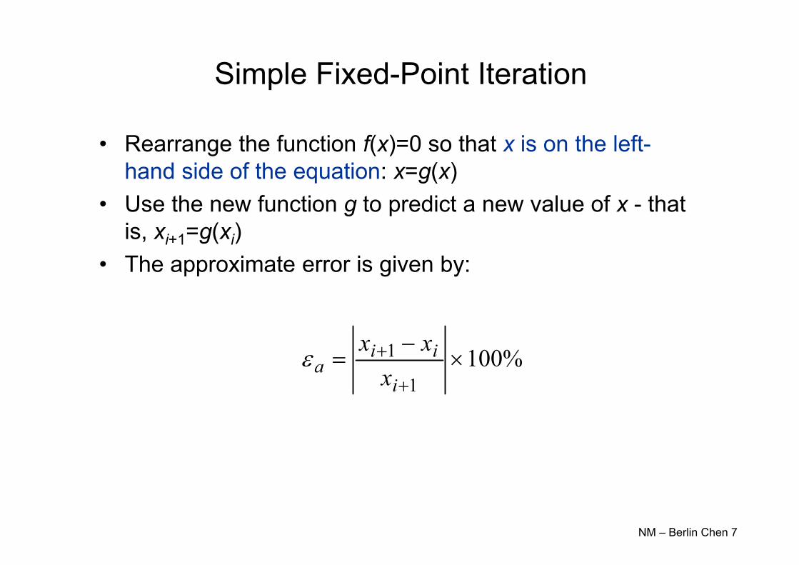
Simple Fixed-Point Iteration
• Rearrange the function f(x)=0 so that x is on the left-hand side of the equation: x=g(x)
• Use the new function g to predict a new value of x - that is, xi+1=g(xi)
• The approximate error is given by:
NM – Berlin Chen 7
%100 1
1
i
iia x
xx
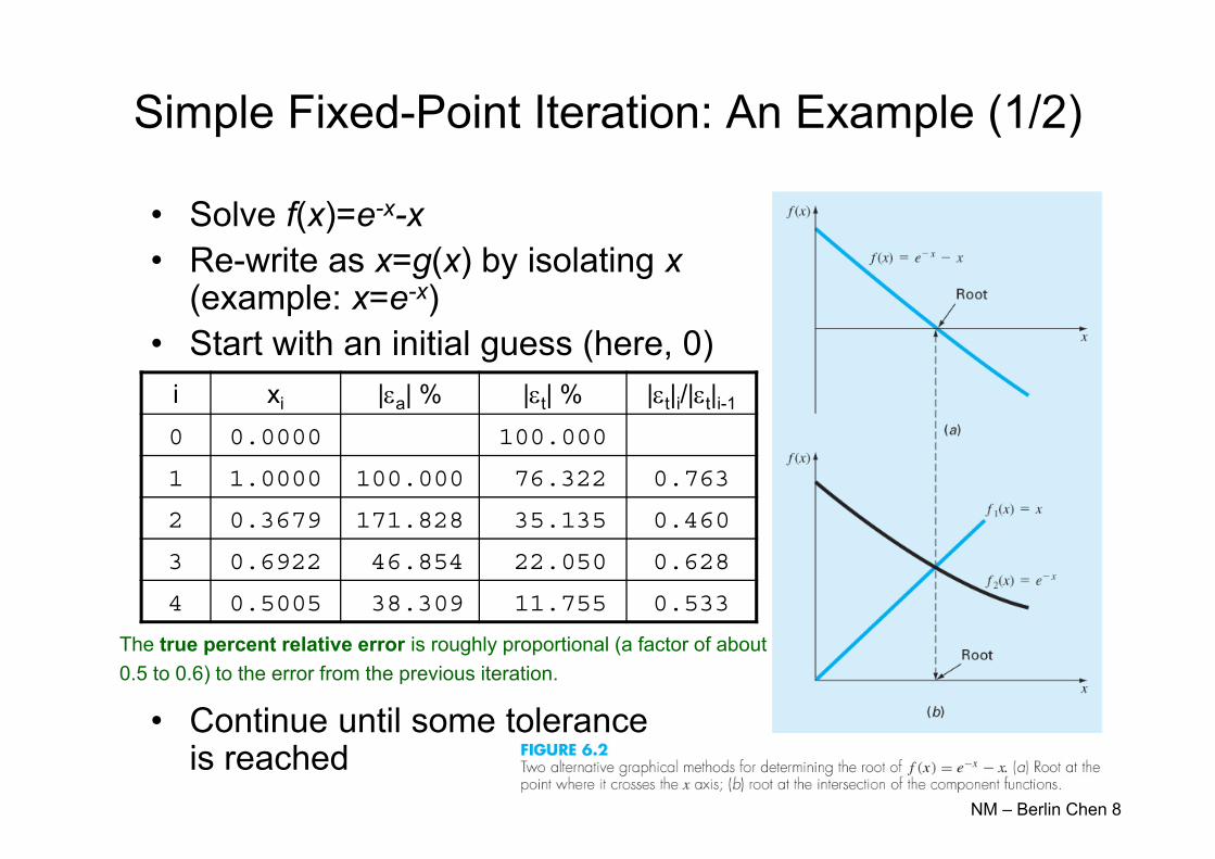
Simple Fixed-Point Iteration: An Example (1/2)
• Solve f(x)=e-x-x• Re-write as x=g(x) by isolating x
(example: x=e-x)• Start with an initial guess (here, 0)
• Continue until some toleranceis reached
NM – Berlin Chen 8
i xi |a| % |t| % |t|i/|t|i-10 0.0000 100.000
1 1.0000 100.000 76.322 0.763
2 0.3679 171.828 35.135 0.460
3 0.6922 46.854 22.050 0.628
4 0.5005 38.309 11.755 0.533
The true percent relative error is roughly proportional (a factor of about 0.5 to 0.6) to the error from the previous iteration.

Simple Fixed-Point Iteration: An Example (2/2)
NM – Berlin Chen 9
0x 1x2x 3x

Convergence
• Convergence of the simple fixed-point iteration method requires that the derivative of g(x) near the root has a magnitude less than 11) Convergent, 0≤g’<12) Convergent, -1<g’≤03) Divergent, g’>14) Divergent, g’<-1
NM – Berlin Chen 10 ii EgE 1
Chapra and Canale (2010) have shown that the error for any iteration is linearly proportional to the error from the previous iteration multiplied by the
absolute value of the slope (derivative) of g(x):
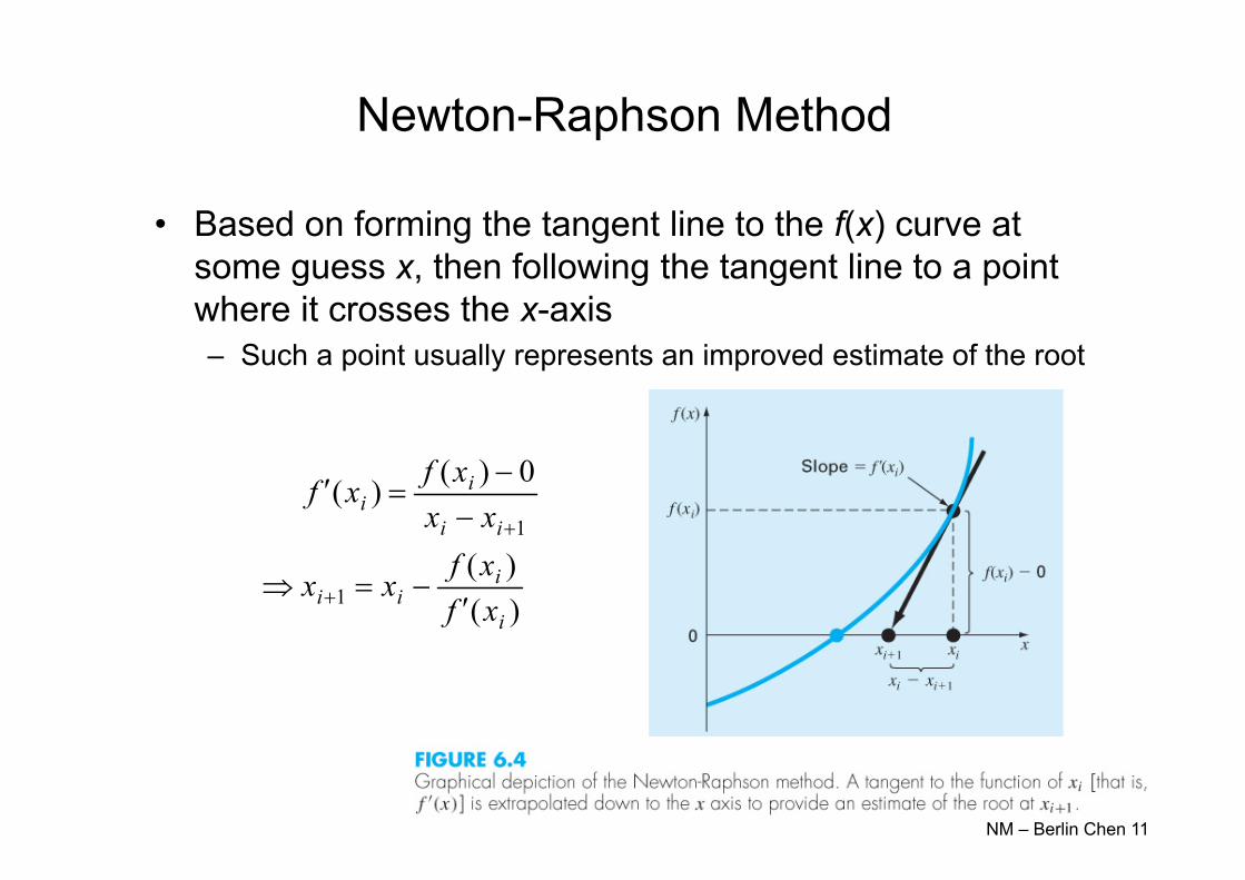
Newton-Raphson Method
• Based on forming the tangent line to the f(x) curve at some guess x, then following the tangent line to a point where it crosses the x-axis– Such a point usually represents an improved estimate of the root
NM – Berlin Chen 11
)()(
0)()(
1
1
i
iii
ii
ii
xfxfxx
xxxfxf
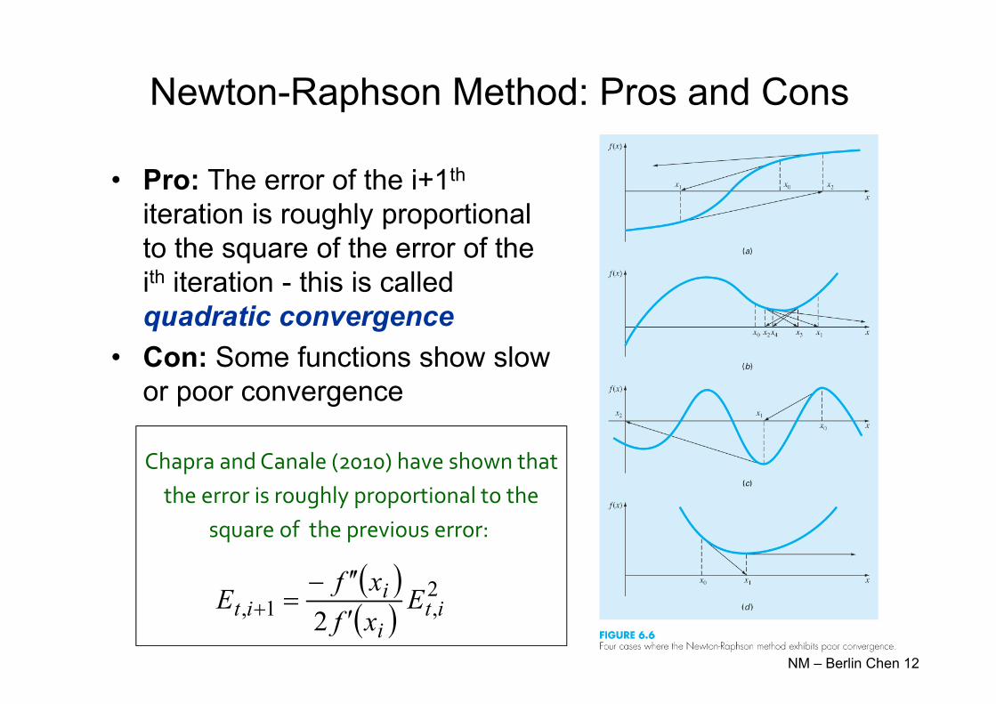
Newton-Raphson Method: Pros and Cons
• Pro: The error of the i+1th
iteration is roughly proportional to the square of the error of the ith iteration - this is called quadratic convergence
• Con: Some functions show slow or poor convergence
NM – Berlin Chen 12
Chapra and Canale (2010) have shown thatthe error is roughly proportional to the
square of the previous error:
2,1, 2 it
i
iit E
xfxfE

Secant Methods (1/2)
• A potential problem in implementing the Newton-Raphson method is the evaluation of the derivative -there are certain functions whose derivatives may be difficult or inconvenient to evaluate
• For these cases, the derivative can be approximated by a backward finite divided difference:
NM – Berlin Chen 13
f ' (xi) f (xi1) f (xi)xi1 xi
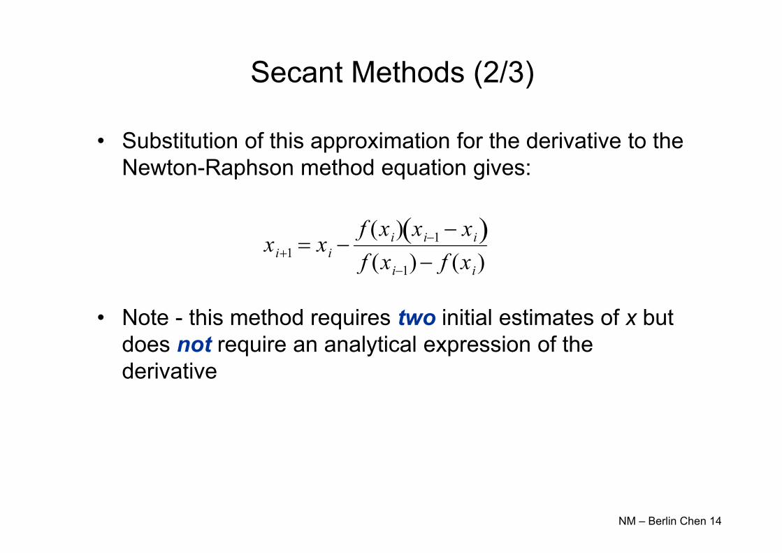
Secant Methods (2/3)
• Substitution of this approximation for the derivative to the Newton-Raphson method equation gives:
• Note - this method requires two initial estimates of x but does not require an analytical expression of the derivative
NM – Berlin Chen 14
xi1 xi f (xi) xi1 xi f (xi1) f (xi)

Secant Methods (3/3)
• Modified Secant Method– Rather than using two arbitrary values to estimate the derivate,
an alternative approach involves a fractional perturbation of the independent variable to estimate f’(x)
NM – Berlin Chen 15
)()()(
)()()(
1iiii
iiii
i
iiiii
xxfxxfxfxxx
xxxfxxfxf

Brent’s Root-location Method
• A hybrid approach that combines the reliability of bracketing with the speed of open methods– Try to apply a speedy open method whenever possible, but
revert to a reliable bracketing method if necessary• That is, in the event that the open method generate an
unacceptable result (i.e., an estimate falling outside the bracket), the algorithm reverts to the more conservative bisection method
– Developed by Richard Brent (1973)
• Here the bracketing technique being used is the bisection method, whereas two open methods, namely, the secant method and inverse quadratic interpolation, are employed – Bisection typically dominates at first but as root is approached,
the technique shifts to the fast open methodsNM – Berlin Chen 16

Inverse Quadratic Interpolation (1/4)
• Inverse quadratic interpolation is similar in spirit to the secant method– The secant method: compute a straight line that goes through
two guesses and take the intersection of the straight line with the x axis as the new root estimate
– Inverse quadratic interpolation: compute parabola (quadratic curve), a function of x, that goes through three points and take the intersection of the parabola with the x axis as the new root estimate
• However, it is possible that the parabola might not intersect the x axis
• Inverse quadratic interpolation rectifies the difficulty by fitting the points with a parabola in y (a function of y)
NM – Berlin Chen 17
iiiii
iii
iiii
iii
iiii
ii xyyyyyyyyx
yyyyyyyyx
yyyyyyyyyg
))(())((
))(())((
))(())((
12
121
121
22
212
1
This form is also called a Lagrange polynomial.

Inverse Quadratic Interpolation (2/4)
NM – Berlin Chen 18
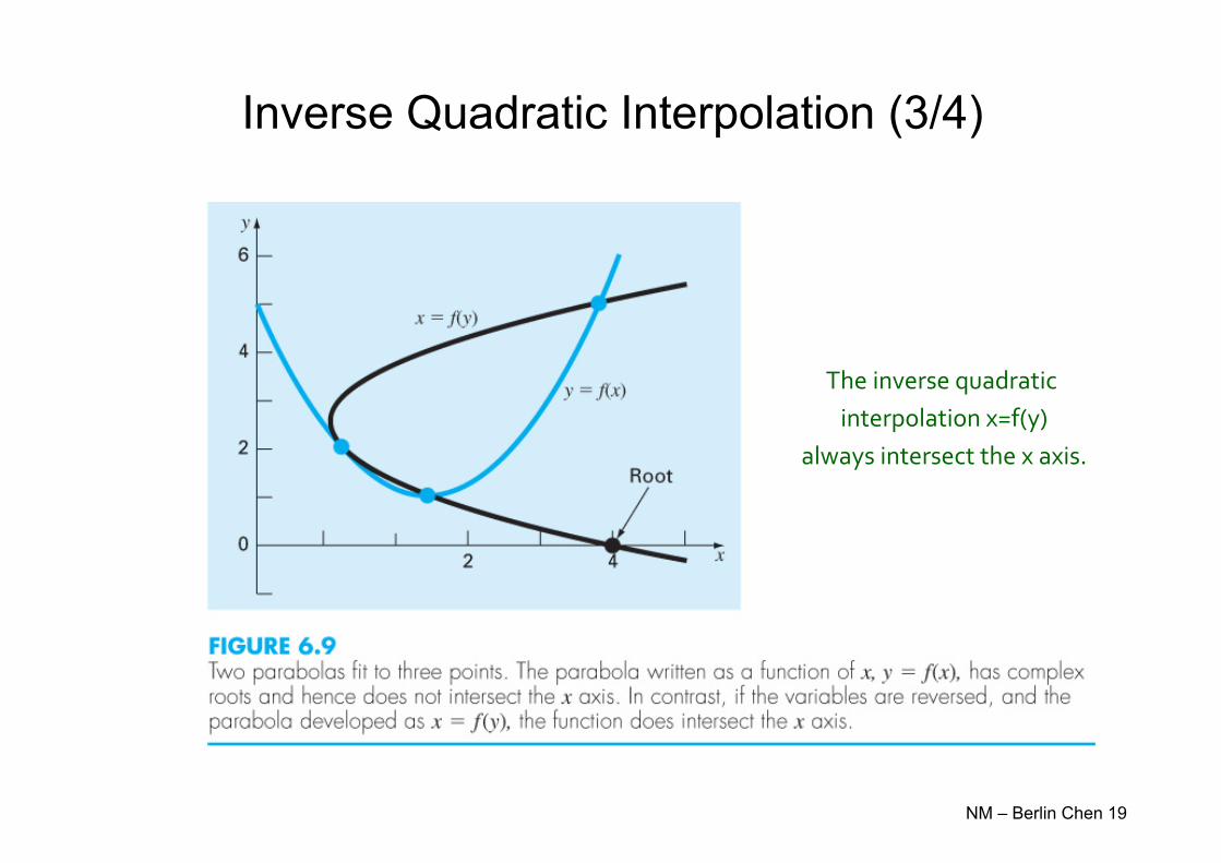
Inverse Quadratic Interpolation (3/4)
NM – Berlin Chen 19
The inverse quadratic interpolation x=f(y)
always intersect the x axis.

Inverse Quadratic Interpolation (4/4)
• The new root estimate, xi+1, therefore corresponds to y=0-Substituted into the equation shown above, we can have
NM – Berlin Chen 20
iiiii
iii
iiii
iii
iiii
iii x
yyyyyyx
yyyyyyx
yyyyyyx
))(())(())((
12
121
121
22
212
11
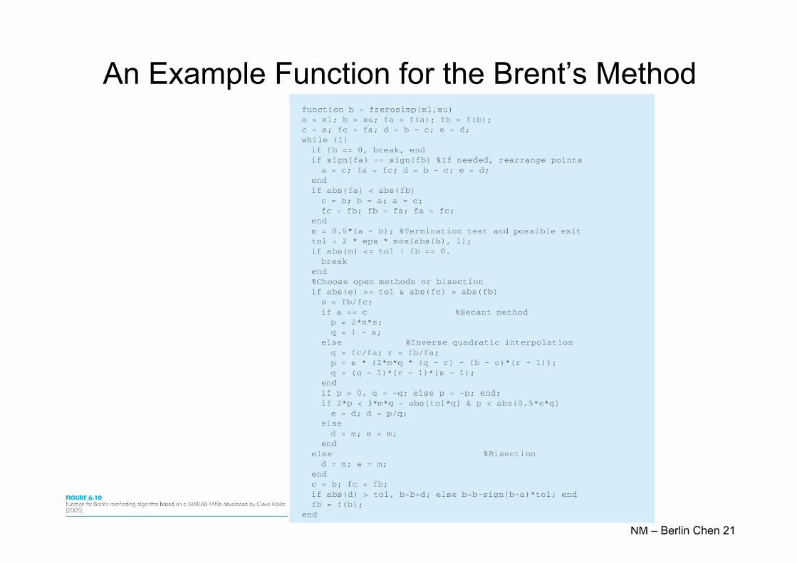
An Example Function for the Brent’s Method
NM – Berlin Chen 21

MATLAB’s fzero Function
• MATLAB’s fzero provides the best qualities of both bracketing methods and open methods.– Using an initial guess:x = fzero(function, x0)[x, fx] = fzero(function, x0)• function is a function handle to the function being
evaluated• x0 is the initial guess• x is the location of the root• fx is the function evaluated at that root
– Using an initial bracket:x = fzero(function, [x0 x1])[x, fx] = fzero(function, [x0 x1])
• As above, except x0 and x1 are guesses that must bracket a sign change
NM – Berlin Chen 22

fzero Options
• Options may be passed to fzero as a third input argument - the options are a data structure created by the optimset command
• options = optimset(‘par1’, val1, ‘par2’, val2,…)
– parn is the name of the parameter to be set– valn is the value to which to set that parameter– The parameters commonly used with fzero are:
• display: when set to ‘iter’ displays a detailed record of all the iterations
• tolx: A positive scalar that sets a termination tolerance on x
NM – Berlin Chen 23
fzero Example
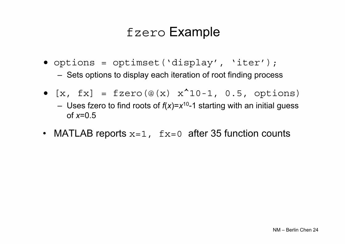
• options = optimset(‘display’, ‘iter’);– Sets options to display each iteration of root finding process
• [x, fx] = fzero(@(x) x^10-1, 0.5, options)– Uses fzero to find roots of f(x)=x10-1 starting with an initial guess
of x=0.5
• MATLAB reports x=1, fx=0 after 35 function counts
NM – Berlin Chen 24

Polynomials (1/2)
• MATLAB has a built in program called roots to determine all the roots of a polynomial -including imaginary and complex ones.
• x = roots(c)– x is a column vector containing the roots– c is a row vector containing the polynomial
coefficients• Example:
– Find the roots of
f(x)=x5-3.5x4+2.75x3+2.125x2-3.875x+1.25
– x = roots([1 -3.5 2.75 2.125 -3.875 1.25]) NM – Berlin Chen 25

Polynomials (2/2)
• MATLAB’s poly function can be used to determine polynomial coefficients if roots are given:– b = poly([0.5 -1])
• Finds f(x) where f(x) =0 for x=0.5 and x=-1• MATLAB reports b = [1.000 0.5000 -0.5000]• This corresponds to f(x)=x2+0.5x-0.5
• MATLAB’s polyval function can evaluate a polynomial at one or more points:– a = [1 -3.5 2.75 2.125 -3.875 1.25];
• If used as coefficients of a polynomial, this corresponds to f(x)=x5-3.5x4+2.75x3+2.125x2-3.875x+1.25
– polyval(a, 1)• This calculates f(1), which MATLAB reports as -0.2500
NM – Berlin Chen 26