Scaling issues in snow hydrology - University of Washingtondepts.washington.edu/mtnhydr/snowschool/Bloschl1999.pdfIn a second step we examine distributed snow models which are a non-linear

Scaling issues in snow hydrology

GuÈ nter BloÈ schl*Institut fuÈr Hydraulik, GewaÈsserkunde und Wasserwirtschaft, Technische UniversitaÈt Wien, Austria

Abstract:The concept of scale can be used to quantify characteristic lengths of (a) a natural process (such as the

correlation length of the spatial snow water equivalent (SWE) variability); (b) a measurement (such as the sizeof a snow density sample or the footprint of a satellite sensor), and (c) a model (such as the grid size of adistributed snow model). The di�erent types of scales are denoted as process scale, measurement scale and

model scale, respectively. Interpolations, extrapolations, aggregations, and disaggregations are viewed as achange in model scale and/or measurement scale.In a ®rst step we examine, in a linear stochastic analysis, the e�ect of measurement scale and model scale on

the data and the model predictions. It is shown that the ratio of the measurement scale and the process scale,and the ratio of the model scale and the process scale are the driving parameters for the scale e�ects. These scalee�ects generally cause biases in the variances and spatial correlation lengths of satellite images, ®eldmeasurements, and simulation results of snow models. It is shown, by example, how these biases can be

identi®ed and corrected by regularization methods. At the core of these analyses is the variogram. For the caseof snow cover patterns, it is shown that it may be di�cult to infer the true snow cover variability from thevariograms, particularly when they span many orders of magnitude.

In a second step we examine distributed snow models which are a non-linear deterministic approach tochanging the scale. Unlike in the linear case, in these models a change of scale may also bias the mean over acatchment of snow-related variables such as SWE. There are a number of fundamental scaling issues with

distributed models which include subgrid variability, the question of an optimum element size, and parameteridenti®ability. We give methods for estimating subgrid variability. We suggest that, in general, an optimumelement size may not exist and that the model element scale may in practice be dictated by data availability and

the required resolution of the predictions. The scale e�ects in distributed non-linear models can be related to thelinear stochastic case which allows us to generalize the applicability of regularization methods. While most ofthe paper focuses on physical snow processes, similar conclusions apply and similar methods are applicable tochemical and biological processes. Copyright # 1999 John Wiley & Sons, Ltd.

KEY WORDS scale; scaling; aggregation; snow cover patterns; regularization; distributed snow models; fractals;e�ective parameters; representative elementary area; subgrid variability; snow water equivalent

INTRODUCTION

This paper addresses two questions: (1) How can we measure and represent snow processes at di�erentscales? and (2) How can we aggregate and disaggregate spatial snow data?; These are very broad questionsindeed and have rami®cations in three main areas of snow hydrology: (i) In the quest for revealing the truenature of snow processes, more speci®c questions include: What is the nature of spatial snow variability?

CCC 0885±6087/99/142149±27$17�50 Received 23 September 1998Copyright # 1999 John Wiley & Sons, Ltd. Revised 8 January 1999

Accepted 11 March 1999

HYDROLOGICAL PROCESSESHydrol. Process. 13, 2149±2175 (1999)

*Correspondence to: Assoc. Prof. GuÈ nter BloÈ schl, Institut fuÈ r Hydraulik, GewaÈ sserkunde und Wasserwirtschaft, TechnischeUniversitaÈ t Wien, Karlsplatz 13/223, A-1040 Wien, Austria. E-mail: [email protected]

Contract grant sponsor: United States Army, European Research O�ce.Contract grant number: R&D 8637-EN-06.

and: How does it change with scale? (ii) In the context of measurements and data collection more speci®cquestions include: At which scale should we measure?; How can we interpret data measured at a given scale?;and How can we best design a snow measurement network? (iii) In modelling, there are issues related tospatial estimation in general. For example: How can we interpolate/extrapolate from measurements?; Howcan we aggregate/disaggregate measurements?; or more generally, How can local observations be transferredto larger scales? In modelling, there are also issues related to distributed physically based snow models, suchas How can we represent spatial processes in these models; How can we represent subgrid variability?; andWhat is the optimum model resolution? Clearly, there are more questions here than are likely to be answeredin the near future. This paper attempts to contribute to a more coherent understanding of these issues byproposing a framework within which we can deal with these issues.

On closer examination, and from a more general perspective, most of these issues arise because the scale atwhich the data are collected is di�erent from the scale at which the predictions are needed. Figure 1 shows asketch of how natural snow variability, data and model predictions are related in general. At the top ofFigure 1 is the true spatial variability, i.e. the true snow hydrological processes which, however, will never beknown in full detail. These natural processes possess certain properties such as spatial patterns of a variable,a true variance, a true correlation length, etc. To obtain information on these processes, measurements aremade, either by data collection of a standard hydrologic network, in research catchments, at study plots orby remote sensing techniques. The measurements produce data. The important thing is that the data will notaccurately portray the natural variability because of a number of factors. Among these factors are instru-ment error (which will not be dealt with in this paper) and the spatial dimensions of the instruments (which isthe focus of this paper). The patterns of the data will be di�erent from the true patterns and so will theirstatistical moments. For example, the variance estimated from the data (i.e. the apparent variance) will, ingeneral, be di�erent from the true variance. In a second step, the data are combined by some sort of model toproduce predictions. Again, the predictions will in general be di�erent from the data due to a number offactors related to the properties of the model, such as the spatial dimensions of the model or model elements.The apparent variance of the predictions will, in general, be di�erent from the apparent variance of the data.This situation is a very general framework which is probably applicable to any branch of scienti®c enquiry.Here, we will use this framework to quantify the biases and e�ects of the various space scales involved insnow hydrologic research.

It may be useful to start with a de®nition of scale and scaling. We will adopt the de®nitions proposed byBloÈ schl and Sivapalan (1995) and BloÈ schl (1999). The term `scale' refers to a characteristic length or time.Often, it is used in a qualitative way as in à small scale phenomenon' but here we will use it quantitatively torefer to a space dimension. We will propose a `process scale' that relates to a spatial dimension of naturalvariability (such as the spatial variability of snow water equivalent); a `measurement scale' that relates to a

Figure 1. Scale e�ects in the measurements cause biases in the data; scale e�ects in the models cause biases in the model predictions.Scaling or change of scale is depicted as double arrows

Copyright # 1999 John Wiley & Sons, Ltd. HYDROLOGICAL PROCESSES, VOL. 13, 2149±2175 (1999)

2150 G. BLOÈ SCHL

spatial dimension of an instrument or a measurement structure (such as a snow lysimeter); and a `modelscale' that relates to a spatial dimension of a model in a general sense (such as a distributed snow model).These de®nitions are consistent with the sketch in Figure 1.

We will use the term `scaling', to denote a `change in scale'. In Figure 1, there are two changes in scale,from the true process to the data (i.e. scaling by the measurement); and from the data to the predictions(i.e. scaling by the model). The purpose of this paper is to quantify the e�ects of scaling due to themeasurements and the e�ects of scaling due to the model. Aggregation, disaggregation, extrapolation andinterpolation always imply a change of scale and hence we will subsume these things under the term scaling.It should also be noted that the usage of `scaling' adopted here is one of two usages that can be found in theliterature. The other usage of scaling relates to some sort of similarity or scale invariance such as in `scalingsnowdrift development rate' (Lever and Haehnel, 1995), `scaling Richards equation' (Kutilek et al., 1991) or`scaling in river networks' (Foufoula-Georgiou and Sapozhnikov, 1998). Although we will also touch on theissue of scale invariance in this paper, for clarity, we will strictly use scaling to denote a change of scale only.

There are a number of factors that complicate scaling in snow hydrology. First of all, the extreme spatialvariability of the hydrologic environment greatly complicates the spatial estimation problem (see e.g. Elderet al., 1989). If a snow pack is examined in great detail, the number of possible ¯ow paths for melt water orgas exchange becomes enormous. Along any path the shape, slope and boundary roughness may be chang-ing continuously from place to place and these factors also vary in time as the snow becomes wet. Similarcomplexity occurs at the catchment and the regional scales. Because of these complications, it is not possibleto describe some hydrologic processes with exact physical laws. The scale at which a conceptualization isformulated then becomes critically important and the transfer of information across scales becomes verydi�cult. Second, when seeking a quantitative description of the natural system one must either adopt adeterministic or a stochastic framework (or a combination thereof). If the spatial patterns of the hydrologicprocess are `consistent' enough (i.e. exhibit òrganization') a deterministic analysis is warranted while for alarge degree of disorder (i.e. `randomness') there is usually merit in probabilistic treatment. Unfortunately,hydrologic processes show elements of both chance and structure which complicates both types of analyses(BloÈ schl et al., 1993). Closely related to organization is the non-linear behaviour of snow processes thatcomplicates scale issues. Third, in many instances there is an enormous contrast in scale between theavailable data and the prediction required, which may exceed several orders of magnitude. This largecontrast may imply that di�erent processes become operative at di�erent scales, and empirical expressionsderived for the smaller scale no longer hold true at the larger scale (see e.g. Seyfried and Wilcox, 1995).Clearly, one would not expect processes that control crystal growth at the millimetre scale to be alsoimportant at the regional scale where climatic e�ects are probably more relevant.

There have been a number of reviews of scale issues in hydrology in general (e.g. BloÈ schl and Sivapalan,1995) and a number of collection of papers of conference proceedings on the same topic (e.g. RodrõÂ guez-Iturbe and Gupta, 1983; Gupta et al., 1986; Kalma and Sivapalan, 1995; BloÈ schl et al., 1997). Here, we willbuild on this work with a focus on snow hydrology.

THE CONCEPT OF SCALE

Process scale

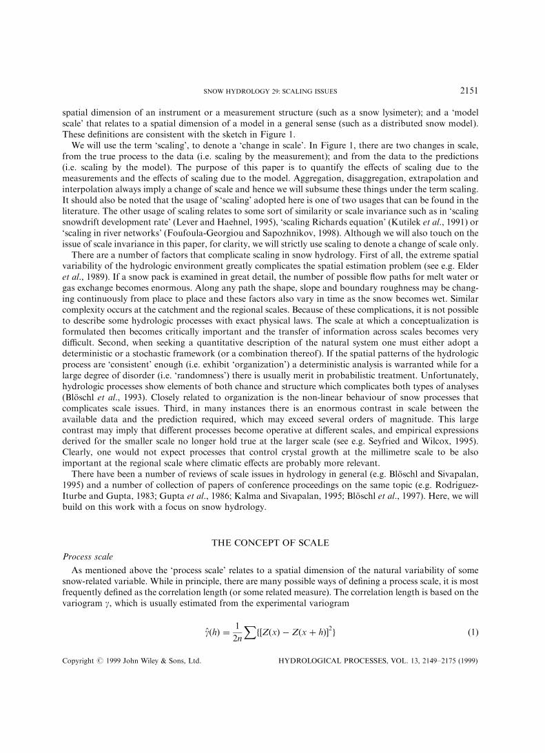
As mentioned above the `process scale' relates to a spatial dimension of the natural variability of somesnow-related variable. While in principle, there are many possible ways of de®ning a process scale, it is mostfrequently de®ned as the correlation length (or some related measure). The correlation length is based on thevariogram g, which is usually estimated from the experimental variogram

g�h� � 1

2n

Xf�Z�x� ÿ Z�x � h��2g �1�


SNOW HYDROLOGY 29: SCALING ISSUES 2151

where Z are the data (such as snow water equivalent (SWE) or snow depth data) at locations x and x � h,and h is the distance or lag between two data points. In equation (1), the lag h is subdivided into classes, thesummation refers to an individual class and n is the number of data pairs for each class. The experimentalvariogram is usually ®tted by some analytical function (in the processes of inferring the population statisticsfrom the sample statistics) such as an exponential function of the form

g�h� � s2�1 ÿ exp�ÿh=l�� 2�where s2 is the (spatial) variance of Z and l is the correlation length (Figure 2a). In some instances, theintegral scale I is used instead of the correlation length, which is de®ned as

I �Z 10

1 ÿ g�x�s2

dx �3�

For an exponential variogram (equation (2)) the integral scale is equal to the correlation length. For di�erenttypes of variograms, the integral scale may be a more objective measure of the process scale than thecorrelation length.

The correlation length (or integral scale) can, strictly speaking, only be derived for a stationary process.For a stationary process, the variogram ¯attens out at large lags h (as shown in Figure 2a), which implies thata variance exists. For a non-stationary process, the variogram keeps increasing with large scales. Hence, thevariance approaches in®nity and the correlation length (or integral scale) also approaches in®nity or does notexist. However, it is sometimes possible to assume local stationarity (i.e. the variogram ¯attens out at somelag after which it increases) as a working hypothesis, in which case a correlation length (or integral scale) canbe estimated.

The correlation length (or integral scale) is a measure of the average distance over which the variable iscorrelated. Equation (2) suggests that for distances shorter than the correlation length the correlations arebetter than r2 � 0.37 where r2 is the coe�cient of determination. Indeed, the process scale (correlationlength) captures the scale of the continuity of a natural variable such as SWE. If the variable is verycontinuous, i.e. varies smoothly in space, the process scale is large. If the variable is discontinuous, i.e. withrapid ¯uctuations over short distances, the process scale is small. A smoothly varying variable will exhibit

Figure 2. (a) De®nition of the process scale (correlation length, l, or integral scale, I). (b) De®nition of the measurement scale and themodel scale. The scale triplet (spacing, extent and support) can apply to measurements and to models. From BloÈ schl and Sivapalan

(1995)


2152 G. BLOÈ SCHL

large uniform patches in space while a rapidly ¯uctuating variable will exhibit small uniform patches. Forexample, the process scale of snow covered area (a binary variable snow covered/snow free) is directlyproportional to the average size of the snow free and snow covered patches. More details on the variogramand on correlation scales can be found in the extensive literature on geostatistics (e.g. Journel and Huijbregts,1978; Isaaks and Srivastava, 1989).

Measurement scale

Following BloÈ schl and Sivapalan (1995) we suggest that the measurement scale consists of a scale triplet:spacing, extent, and support (Figure 2b). `Spacing' refers to the distance between samples; èxtent' refers tothe overall coverage of the data; and `support' refers to the integration volume or area of the samples. Allthree components of the scale triplet are needed to uniquely specify the space dimensions of a measurementor instrumental setup. For example, for a snow course the scale triplet may have typical values of, say, 100 mspacing (between the samples), 1 km extent (i.e. the length of the course), and 10 cm support (the diameter ofthe snow density probe). Similarly, for a remotely sensed image, the scale triplet may have typical values of,say, 30 m spacing (i.e. the pixel size), 10 km extent (i.e. the overall size of the image), and 20 m support(i.e. the `footprint' of the sensor). The footprint of the sensor is the area over which it integrates theinformation to record one pixel value. It is usually on the order of the pixel size but not necessarily identicalto it.

In the two-dimensional case it is sometimes useful to relate the spacing, the extent, and the support toareas which is a logical extension from the one-dimensional case in Figure 2b:

aSpac ��Aregion=n

q�4�

aExt ��Aregion

q�5�

aSupp ��Aaggreg

q�6�

where aSpac , aExt , and aSupp are the spacing, the extent, and the support respectively. Aregion is the overall sizeof the region of interest, n is the number of samples in this region, and Aaggreg is the area over which a sampleaggregates (or integrates). This paper will focus on the two dimensional case.

Model scale

Again following BloÈ schl and Sivapalan (1995) we suggest that the model scale consists of a scale triplet(spacing, extent, and support, Figure 2b) very similar to that of the measurement scale. The di�erence is thatthe model scale is related to the spatial properties of the model (in a general sense) rather than those of themeasurements. For example, for a spatially distributed snow model the scale triplet may have typical valuesof, say, 25 m spacing (i.e. the grid size), 1 km extent (i.e. the size of the catchment to be modelled), and 25 msupport (the grid size). The support is the spatial dimension over which the variables in each grid cell arerepresentative which is equal to the grid size in most distributed models. In regional mapping (which is amodel in a general sense) of snow depths the scale triplet may have typical values of, say, 10 m spacing(i.e. the resolution to which the map is produced), 10 km extent (i.e. the overall size of the map), and 10 cmsupport (which is the area which each point in the map is representative of). In this example, the map showspoint values of snow depths (rather than averaged values), hence the support is very small. The support inmaps is sometimes termed `grain'. Clearly, it is possible to draw two maps of, say, snow depth of the samearea, one map showing point values (very small support) and the other map showing values averaged over acertain area (i.e. larger support). The latter map will be smoother than the former.



Scaling

Here we are interested in the change of the scale, i.e. how will the measurement spacing, extent and supportchange the true pattern to be re¯ected in the data; and how will the model spacing, extent and supportchange the data to be re¯ected in the predictions (Figure 1). The basic idea of BloÈ schl and Sivapalan (1995)and BloÈ schl (1999) is that there is some similarity between these two steps. Generally, if the spacing of thedata is too large, the small scale variability will not be captured. If the extent of the data is too small, thelarge scale variability will not be captured and will translate into a trend in the data. If the support is toolarge, most of the variability will be smoothed out and the data will appear very smooth. It is clear that somesort of ®ltering is involved, i.e. the true patterns are ®ltered by the properties of the measurement which isre¯ected in the data. It is also clear for dimensional reasons that the e�ect of the ®lter will be closely relatedto the ratio of the measurement scale and the process scale. So, more strictly speaking, we should say that Ìfthe spacing of the data is too large as compared to the process scale, the small scale variability will not becaptured'. Analogous statements apply to the extent and the support. The model scale has similar e�ects. Ifthe spacing of the model elements is too large as compared to the process scale, most of the variability willappear as noise in the predictions. Analogous results apply to the extent and the support of the model. Thischange of scale, conceptualized as a ®lter, has been quantitatively discussed in Cushman (1984, 1987), Beckie(1996), Federico and Neuman (1997) and BloÈ schl (1999), and a more general discussion is provided inBloÈ schl and Sivapalan (1995).

There are a number of ways of conceptualizing the ®lters mentioned above. These can be linear ®lters ornon-linear ®lters; and the analysis can be moulded in a stochastic framework or in a deterministic frame-work. In snow hydrology, out of the four possible combinations, the two most important ones are a linearstochastic analysis (i.e. mainly geostatistics) and a non-linear deterministic analysis (i.e. mainly distributedphysically-based modelling). We will discuss these two most important cases in the following sections.

LINEAR STOCHASTIC ANALYSIS

Framework

There are two fundamental assumptions on which this type of analysis rests:First, the process is linear, i.e. it aggregates linearly or, in other words, simple arithmetic averaging applies:

E�f�x�� f�E�x�� 7�

where E is the mathematical expectation, x is location and f is a function or a variable. In snow hydrologythere are many processes that do average linearly and many other processes that do not. If f is a variable,linear averaging is applicable if a conservation law (of mass or energy) holds. For example, if we measureSWE at a 1 m grid in a catchment and calculate the total SWE volume in the catchment from this and, in asecond step, aggregate the measurements to a 10 m grid and, again calculate that total SWE in thecatchment, these two methods will give the same results due to conservation of mass. In this example, x inequation (7) relates to the 1 m grid coordinates, E(x) to the 10 m grid coordinates, f(x) is SWE at the 1 mgrid, f(E(x)) is SWE at the 10 m grid, and E( f(x)) is SWE at the 1 m grid averaged over 10� 10 m. However,if we aggregate snow albedo to di�erent grid sizes in a physically realistic manner, the average values over thecatchment of the two methods will not necessarily be the same. This is because snow albedo is not con-servative. If f is a function representing a measurement set up, there are instruments that do average linearly(such as a raingauge), there are instruments that average linearly in good approximation (such as TDR orsatellite sensors), and there are instruments that aggregate non-linearly. If f is a function in a modelrepresenting a hydrologic process (such as Darcy's law), then unfortunately equation (7) often does notapply as most hydrologic processes do not average linearly. In Darcy's law, for example, the averagehydraulic conductivity over an area does not give the average ¯ux over the same area, i.e. equation (7) does


2154 G. BLOÈ SCHL

not hold. In such cases one may resort to non-linear stochastic analyses (e.g. Gelhar, 1993) or to non-lineardeterministic models (see later in this paper).

The second assumption is that the variable to be examined is a second order stationary random variable.Random means that any sort of organization that may be present in the spatial patterns may be neglected. Itis clear that catchments are highly organized and, often, snow processes show (organized) linear features.However, in a ®rst approximation it may be useful to assume that snow processes are random in space and toneglect other controls. The assumption of second order stationarity essentially implies that the variogram(equation (1)) does not change with location in the catchment or in the region. It does not necessarily implystationarity (in the mean), i.e. there is no need that the variogram ¯attens out at some lag. Second orderstationarity may be a reasonable assumption in many applications. However, in some applications, such asnetwork planning, the assumption of second order stationarity does not make sense. In a stochasticapproach to network planning the idea is usually that regions with small scale variability (small processscale) are densely sampled (small spacing) while regions with large scale variability are less densely sampled.Clearly, this is inconsistent with the assumption that the variogram (and hence the process scale) does notchange with location.

Based on these two assumptions we can now apply standard geostatistics (e.g. Journel and Huijbregts,1978) or, equivalently, linear ®ltering theory for random ®elds (Wiener, 1966) to obtain a ®ltered random®eld, i.e. a random ®eld obtained from aggregating, disaggregating, extrapolating or interpolating datapoints. As mentioned above, aggregation, disaggregation, extrapolation and interpolation (i.e. a change ofscale by the measurement or the model) can be viewed as ®ltering. We will not go into the details of thistheory here, which are contained in a rich literature on the subject (see e.g. Journel and Huijbregts, 1978;Vanmarcke, 1983; Isaaks and Srivastava, 1989; Journel, 1993; Armstrong, 1998). We will only present someof the results that are most relevant to snow hydrology in an intuitive way. There are three main results onewould be interested in and that can be obtained from geostatistics: (a) the most likely spatial pattern of thevariable of interest, (b) spatial patterns with the most realistic variability, and (c) the moments of thepatterns. For (a) there are a wide range of geostatistical interpolation methods (kriging and varieties thereof)that are also able to handle the e�ect of support (e.g. block kriging). These are best linear unbiasedestimators that, however, have the disadvantage of tending to smooth out the patterns, i.e. the interpolatedpatterns are smoother than the real ones. There is a class of interpolators that do not smooth the patternsthat are termed stochastic simulations (b). However, this is at the expense of not producing the best inter-polations. Stochastic simulations (such as sequential indicator simulation and others) produce a number ofequally likely realizations of the patterns, each of them having the same spatial variability (i.e. variogram) asthe true pattern. There are software packages available for both classes of methods (e.g. GSLIB, Deutschand Journel, 1997; SURFER, Golden Software, 1998). In this paper, for clarity, we will focus on (c), i.e. thestatistical moments, and how they change with scale. The statistical moments we examine are the mean,E( . ), the spatial variance, s2, and the correlation length, l. Speci®cally, we will examine which biases will beintroduced by a change of scale but we will not examine the random errors (estimation variance or reliability)introduced by a change of scale.

Regularization

There are a range of methods for estimating the ®ltered moments. These include (a) the spectral method(where the random function is multiplied with the ®lter function in the frequency domain); (b) ®ltering in thespace domain (simply by running a moving average ®lter over the data, and estimating the moments from the®ltered data); and (c) ®ltering in the lag domain (i.e. by multiplying the variogram by some function) which isusually termed regularization in geostatistics. All of these methods produce very similar results and theirdi�erences are mainly of a methodological nature (Vanmarcke, 1983). Here we will adopt the lag domainapproach (i.e. regularization) which is the one most frequently used in geostatistics. We adopt this approachbecause it is simple and intuitive and consistent with the variogram representation of variability used in theremainder of this paper.



The results presented here are based on standard regularization methods with a number of additionalsimplifying assumptions. In the case of support the variogram of an averaged process is calculated using thevariogram of the point process and a ®lter function. The ®lter is represented by a square of side length aSupp ,which is the support. The square is the area over which the aggregation takes place. Di�erent shapes of thisarea do not signi®cantly a�ect the results of the regularization (RodrõÂ guez-Iturbe and MejõÂ a, 1974). In thecase of spacing, the apparent variogram is approximated by the true variogram for lags larger than thespacing aSpac and by a linear increase from the origin for shorter lags. This assumption is made because whenestimating the empirical variogram there are only a small number of pairs of points for lags smaller than thespacing (Russo and Jury, 1987) and a straight line is the simplest approximation. Discussions of work relatedto this assumption are given in Russo and Jury (1987) and Gelhar (1993). In the case of extent, the apparentvariogram is based on the true variogram for small lags ( for g�h�4s2app�, and is constant and equal to s2appfor large lags. The apparent integral scale, Iapp , is then calculated from the apparent variogram by usingequation (3). Western and BloÈ schl (1999) showed that these assumptions are also reasonable for moregeneral cases. More details on the method are given in Appendix A of Western and BloÈ schl (1999), BloÈ schl(1999), and in most geostatistical texts. Here we will show the results for two types of variograms: anexponential variogram (equation (2)), and a double exponential nested variogram of the form

g �XNi�1

s2i �1 ÿ exp�ÿh=li�� 8�

with N � 2, s21 � 0�3, s22 � 0�7, l1 � 0.1, and l2 � 10. The variogram in equation (8) has two preferredscales, at 0.1 and at 10. From equation (3) we ®nd that the integral scale of this variogram is Itrue � 7�03. Thistype of variogram, with similar parameters, is sometimes used in hydrologic studies spanning a wide range ofscales (e.g. Gelhar, 1993). It is important to reiterate that the ®ltering represents the change of scale (orscaling) and that the e�ect of this change of scale will be controlled by the ratio of the measurement scale(spacing, extent, support) and the process scale, and the ratio of the model scale (spacing, extent, support)and the process scale. It is therefore possible to use non-dimensional quantities such as aSpac=Itrue, i.e. thespacing normalized by the (true) process scale. Similarly, because of linearity, it is possible to non-dimensionalize the apparent variance, s2app (which is the variance of the ®ltered process) by dividing it by thetrue variance, s2true, and to non-dimensionalize the apparent integral scale (or correlation length), Iapp (whichis the integral scale of the ®ltered process) by dividing it by the true integral scale, Itrue .

The results of the regularization analyses are shown in Figure 3. The top left panel of Figure 3 suggeststhat changing the spacing does not change the variance. For example, the SWE estimated from 10 and1000 samples in a catchment will give the same variance, on average. This means that there is no biasintroduced into the variance by a small number of samples but, of course, the estimate of the variance will beless reliable (large random error). No bias implies that the apparent variance is equal to the true variance andhence the ratio of the two quantities (plotted in the top left panel of Figure 3) is unity. Increasing the extent(top centre panel of Figure 3) increases the variance, and increasing the support (top right panel of Figure 3)decreases the variance. The e�ect of extent is consistent with the general observation that as we increase thesize of the domain of interest, additional variability comes in. For example, when we start from the plot scale(say, 1 m2) the spatial variability of snow depth will be very small but as we increase the size of the domain(i.e. the extent) to a mountain range, the variability will increase drastically. For su�ciently large extents theapparent variance is equal to the true variance and hence their ratio approaches unity.

The e�ect of support (top right panel of Figure 3) is consistent with the general observation thataggregation always reduces variance for a random variable. For example, if we compare the SWE at a largenumber of plots in a region, the spatial variability will be quite large. However, if we aggregate the plotvalues to average values in a small number of catchments in the same region, the variability between theaverage catchment values will be much smaller. For su�ciently small supports the apparent variance is equalto the true variance and hence their ratio approaches unity. The reduction of variance with increasing


2156 G. BLOÈ SCHL

support has been recognized in many practical and more theoretical studies in various subdisciplines ofhydrology including rainfall analysis (e.g. areal reduction factors) and regional ¯ood frequency (see e.g.BloÈ schl and Sivapalan, 1997; Sivapalan and BloÈ schl, 1998).

Figure 3 also suggests that increasing the spacing, the extent, and the support will in general increase theapparent integral scale (lower panels). For example, a small number of samples of SWE in a large catchmentanalysed by geostatistical methods (equation (1)) may yield deceptively large correlation lengths, muchlarger than the correlation length of the underlying true snow patterns, because the spacing is large ascompared to the process scale (i.e. true correlation length). On the other hand, correlation lengths estimatedfrom snow lysimeter data at the plot scale are unlikely to capture the large scale variability of snow melt thatis due to large scale topography and climatic conditions and, hence, will underestimate the correlationlengths of the underlying true pattern of snow melt in the region. This result is because the extent is small ascompared to the process scale. Similarly, if we estimate correlation lengths from satellite data at a coarseresolution (i.e. large footprint or support), we will not be able to pick the small scale variability of snow coverpatterns and hence we will overestimate the true correlation lengths.

It should be noted that Figure 3 shows the scale e�ect when changing only one of the scales of the scaletriplet, assuming that the other two do not cause a bias (i.e. spacings are small, extents are large, andsupports are small). The combined scale e�ect of two of the three components of the scale triplet has beenexamined in BloÈ schl (1999) and one example will be given later in this paper.

The e�ect of a change in scale on the mean, E( . ), is not shown in Figure 3. This is because, given theassumption of a linearly aggregating process, a change of scale will not bias the mean. This result indicatesthat irrespective of the spacing, extent, or support of the data (or the model) the mean will always beunbiased, provided the process is linear. If the process model, or the measurement, does not aggregatelinearly then the mean will be biased and may change with the scale. This is examined later in this paper. It

Figure 3. E�ect of spacing, extent and support of a measurement or a model on biases in the variance and the correlation length. s2app isthe apparent variance; s2true is the true variance; Iapp is the apparent integral scale (or apparent correlation length); Itrue is the trueintegral scale (or true correlation length). Based on geostatistical regularization methods (Western and BloÈ schl, 1999). Solid lines are foran exponential variogram (equation (2)) and dashed lines are for a double exponential nested variogram (equation (8)) with the

parameters as in equation (8)



should also be noted that although the mean will not be biased for the case of linear averaging, the reliability(random error) of the mean will obviously change with the scale, but this is beyond the scope of this paper.

Let us consider two examples of how the e�ects depicted in Figure 3 can be used for practical applications.Consider, in the ®rst example, a 10 km2 catchment in which 100 point samples of snow depth have beentaken. From these samples, a correlation length of about 200 m has been estimated by using equations (1)and (2). Question: (a) Is this estimate biased? (b) If so, what is the unbiased correlation length? (c) How manysamples would be needed to obtain an unbiased estimate from the data? Solution: The solution is found bytrial and error. Equation (4) gives aSpac � 320 m. If we assume that the true correlation length is 155 m,aSpac=Itrue � 2�06 for which Figure 3 (bottom left panel) gives Iapp=Itrue � 1�29. This is a solution to the aboveproblem as 1.29*155 m � 200 m which is equal to the apparent correlation length. This is a unique solutionas, assuming, say, Itrue � 180 m gives an estimate of Iapp � 220 m4 200 m while assuming Itrue � 130 mgives an estimate of Iapp � 185 m5 200 m. The correlation length estimated from the samples is biased andthe unbiased correlation length is about 155 m. For an unbiased estimate directly from the data (e.g. errorsmaller than 5%, i.e. Iapp=Itrue 5 1�05� Figure 3 (bottom left panel) indicates that aSpac=Itrue 5 1 which meansthat aSpac5 155 m and at least 420 point samples in space would be needed (equation (4)). It is interesting toexamine the same example for the case of only 10 point samples for which aSpac � 1000 m and Figure 3 doesnot give a solution to the problem. While it is clear that the estimate will be substantially biased it is notpossible to estimate the true correlation length. Clearly, there is not enough information in only ten samples.Similarly, there is no unique solution for apparent correlation lengths much smaller than the spacing which,again is due to the limited amount of information in the data.

Consider a second example of a remotely sensed image that gives some estimate of SWE. In a ®rst step weare interested in the % snow covered area as estimated from this image. Assume that the mean SWE over theimage is 360 mm, the true standard deviation (in space) is 300 mm, and the SWE is distributed according to a(truncated) normal distribution. Assume also that the true correlation length of SWE is Itrue � 100 m, andthe pixel size ( footprint) of the remotely sensed image is 250 m. Question: (a) What is the true snow coveredarea? (b) What% snow covered area would one predict from the remotely sensed image? Solution: (a) For thetrue SWE distribution, the mean is 360/300 � 1.2 times the standard deviation. For a standard normaldistribution, the non-exceedance probability of P�Z5 ÿ 1�2� � 0�12. This means that 12% of the landsurface is snow free and 88% is snow covered. (b) From the remotely sensed image one would predict avariance that is smaller than the true variance. For aSupp=Itrue � 2�5, Figure 3 (top right panel) givess2app;Supp=s

2true � 0�32 which gives an apparent standard deviation of 300*

��0�32p � 170 mm. With this the

mean is 2.1 times the standard deviation and for a standard normal distribution, the non-exceedanceprobability of P�Z5 ÿ 2�1� � 0�02. This means that, from the remotely sensed image, one would predictthat only 2% of the land surface is snow free and 98% is snow covered. Clearly, this misrepresentation willhave a signi®cant e�ect on estimates of the surface energy balance and evapotranspiration. As a side issue itis interesting to examine the apparent correlation length one would estimate from the images. ForaSupp=Itrue � 2�5 one gets Iapp=Itrue � 2�1 from the bottom right panel of Figure 3, hence the apparentcorrelation length is 210 m rather than 100 m. It should also be noted that the numbers in this exampledepend on the assumption of a normal distribution.

Snow cover variograms

So far we have implicitly assumed that (a) the true variograms of the snow cover variables are exponential(equation (2)) and (b) that the true correlation lengths exist and are known a priori. What is the data evidenceon variograms of snow-related variables? Unfortunately, the variables of most interest (such as SWE andsnowmelt) are usually collected at a few points only (e.g. Sommerfeld and Bales, 1993), hence, it is notpossible to estimate variograms spanning many orders of magnitude in scale. Remotely sensed images areuseful but some of the variables derived from them (such as SWE) may not always be reliable. Because ofthis, in this paper we examine snow covered area (SCA), i.e. a binary variable that is 1 for a snow coveredpixel and 0 for a snow free pixel. A large number of snow covered area images are readily available and are


2158 G. BLOÈ SCHL

probably quite reliable. While we do not expect that the variograms of other snow-related variables will beidentical with that of SCA, we do believe that SCA provides very useful insight into the nature of spatialvariability (and variograms) of many snow-related variables, because the driving processes are closelyinterrelated. Patterns of SCA can in fact be interpreted as indicator images of SWE, representing di�erent`thresholds' of SWE at di�erent times of the year. Indicator variograms and indicator geostatistics are widelyused in other areas of hydrology and the geosciences in general where a continuous variable (such as SWE) istransformed into a binary variable by thresholding it (see e.g. Anderson, 1997; Western et al., 1998). Thecorrelation lengths derived from indicator variograms are closely related to the correlation length of thecontinuous variable and are of the same order of magnitude (Deutsch and Journel, 1997). However, ofcourse it is not possible to estimate the variance of the continuous variable from the variance of the indicatorvariable. The variance of the indicator variable, s2

p , is always a function of the mean of the indicator variable.If p is the mean of, say, snow covered area (e.g. p � 0.3, i.e. 30% of the area is snow covered)

s2p � p � �1 ÿ p� �9�

so the variance of the example is 0.21.Sample variograms, estimated by equation (1), from four very di�erent case studies are presented in

Figure 4 as double logarithmic plots. The ®rst set of variograms (Figure 4a) has been derived from a number

Figure 4. Variograms of snow covered area (SCA), i.e. a binary variable that is 1 for a snow covered pixel and 0 for a snow free pixel. (a)Thin sections of snow (eight images for di�erent snow types, pixel size is 0.1 mm); (b) KuÈ htai aerial photographs (nine scenes in 1989,pixel size is 5 m); (c) Sierra Nevada TM images (six scenes in 1997, pixel size is 30 m); (d) Sierra Nevada AVHRR images ( four scenes in

1998, pixel size is 1100 m)



of thin sections obtained in the laboratory by scanning images of snow crystals (R. Davis, pers. comm.).These are binary images where 1 is ice and 0 is void and the pixel size is 0.1 mm. Figure 4a shows that thevariograms are all stationary, i.e. a correlation length exists and is on the order of 0.2 to 0.5 mm. Thedi�erences in the correlation lengths for the di�erent images are mainly due to di�erent types of snow. Theshape of all variograms is close to exponential (equation (2)).

The second set of variograms (Figure 4b) has been derived from aerial photographs in the KuÈ htaicatchment, Austria (BloÈ schl and Kirnbauer, 1992). The boundaries between snow covered and snow freeareas were ®rst digitized manually as vectors in the photographs and in a second step were gridded to a pixelsize of 5 m. The variograms (Figure 4b) are probably not stationary but if we assume local stationarity (byneglecting the part of the variogram for lags larger than 500 m) we would get correlation lengths on the orderof 100 m. The variance, s2

p , is a multiplicative factor in variograms (Figure 2a) and hence translates into theintercept in double logarithmic plots. The variograms in Figure 4b have similar slopes but di�erent interceptswhich means that the di�erences between the variograms are mainly due to di�erences in s2

p and hence due todi�erences in the % snow covered area (equation (9)).

The third set of variograms (Figure 4c) has been derived from Landsat Thematic Mapper (TM) images inthe Sierra Nevada region (see Cline et al., 1998a; Rosenthal and Dozier, 1996) with a pixel size of 30 m. Thevariograms are clearly not stationary as they do not ¯atten out at large lags over the range shown. Most ofthem can be closely approximated by a straight line in the double logarithmic plots which implies that theyconform to a power law. The di�erences between the variograms are partly due to di�erences in the % snowcovered area (equation (9)) which cause the vertical shifts in Figure 4c. However there are also di�erences inthe slope which may be related to other factors such as changes in shading due to variable illumination anglein rugged terrain.

The fourth set of variograms (Figure 4d) has been derived from AVHRR images in the Sierra Nevadaregion (K. Elder, pers. comm.) with a pixel size of 1100 m. The variograms have a di�erent shape than those inFigures 4a, 4b, and 4c. They are approximately stationary as they do not increase for lags larger than 100 km.However, they are not exponential and can be approximated by a straight line between lags of 3 km and100 km. If we were to estimate correlation lengths from Figure 4d, they would be on the order of 30 km. Thedi�erences between the variograms in Figure 4d are mainly due to di�erences in the % snow covered area.

While the variograms in Figures 4a, 4b, 4c and 4d do not apply to the same date and the same location it isreasonable to assume that their general shape will be similar for other dates and locations. Their maindi�erence then is the scale at which the snow cover data have been collected. Given the various biasesintroduced by the sensors in terms of their spacing, extent and support one wonders what the true variogramspanning more than nine orders of magnitude from the crystal to the regional scale would look like, i.e. thevariogram that arises from a combination of the variograms at the four scales. There is an apparentinconsistency in the correlation lengths (Figure 4a: l � 0.0005 m; Figure 4b: l � 100 m; Figure 4d:l � 30 000 m) and it would be interesting to ®nd out whether it is possible to reconcile the variograms shownin Figure 4.

There are two philosophies in the literature on this issue. The ®rst philosophy (e.g. Dagan, 1986; Neuman,1990, 1993; Lovejoy and Schertzer, 1985) suggests that there is some universal continuous variogram that canbe represented by a power law of the form

g � a � hb �10�which is termed a variogram of a fractal and represents scale invariant (or self similar) behaviour.Equation (10) implies non-stationarity. This philosophy is consistent with data evidence when combining alarge number of situations and case studies in hydrology. However, it is hard to understand what would be theactual processes giving rise to one continuous relationship. In other words, equation (10) relates the variabilityat the crystal scale to the variability at the regional scale and from a physical perspective one would not expectthem to be related. The second philosophy (e.g. Gelhar, 1993, p. 295) suggests that there is a discontinuousvariogram exhibiting steps of the form of equation (8). This variogram exhibits a number of preferred scales


2160 G. BLOÈ SCHL

(i.e. the li) each of which may represent one physical process. For example, the process scale of crystal growthmay be l1 � 1 mm, that of wind drift at hillslopes may be l2 � 1 m, that of solar radiation e�ects at hillslopesof di�erent aspects may be l3 � 100 m, and that of di�erent climatic conditions may be l4 � 10 km. Thecombined nested variogram (equation (8)) then is a combination of the e�ects of the individual processes. It islocally stationary because it ¯attens out between the preferred scales. This interpretation is appealing becauseit is consistent with physical reasoning. For example, the thin sections in Figure 4a are stationary and this maybe due to the presence of crystal growth processes only (such as equilibrium processes and kinetic processes)but no other (larger scale) processes (such as the formation of preferential ¯ow ®ngers). On the other hand, aswe increase the scale, larger scale processes are re¯ected in the snow cover data.

Perhaps one possible way of reconciling these two philosophies is by noting that the ensemble mean of alarge number of nested variograms of the type of equation (8) with di�erent sets of li for di�erent casestudies may indeed combine to give an envelope that looks like the fractal in equation (10). For a particularcase study it may be preferable to assume local stationarity at each of the scales mentioned as a workinghypothesis. If the study does not span too many orders of magnitude, the assumption of a stationaryvariogram of the exponential type (equation (2)) or a similar variogram may therefore be appropriate whichimplies the existence of one correlation length. If the study spans more than, say, three orders of magnitude,a nested variogram (equation (8)) may be preferable as it is likely that a number of processes are operative atvery di�erent scales. For both types of variograms the e�ects of scale have been shown in Figure 3 (solid linesand dashed lines, respectively).

As a side issue it may be interesting to examine whether the slope of the variograms in the doublelogarithmic plots (i.e. parameter b in equation (10)) may be a useful parameter for characterizing the spatialsnow cover variability. This is a potential alternative to the correlation length. It would also be interesting toknow whether any relationships to the metamorphic state of the snow cover or other physical controls (suchas the complexity of the terrain) can be detected. For the two dimensional case examined here, the parameterb is related to the Hurst exponent,H, byH � b/2 and to the fractal dimension,D, byD � 3 ÿ b=2 which areparameters that are often used in studies of fractal variability (KlemesÏ , 1974; Feder, 1988; Klinkenberg andGoodchild, 1992). The exponent b is a measure of the ratio of large scale and small scale variability. If b is,say, 1.2 most of the variability occurs at large scales, and if b is, say, 0.1 most of the variability occurs at smallscales. Straight lines have been ®tted to the double logarithmic plots of Figure 4b ( for lags larger than 50 m),Figure 4c, and Figure 4d ( for lags between 3 and 100 km). The slopes of the ®tted lines (i.e. the fractalexponents b, equation (10)) are shown in Figure 5 along with the proportion of snow covered area. Theimages are sorted according to the date they have been collected, i.e. from winter to summer as can be seenfrom the decreasing snow covered area which re¯ects the seasonal snow ablation. The exponent b does notvary much during the year. However, there is a slight tendency towards lower exponents at the end of theablation period. This indicates a larger proportion of small scale variability as compared to large scalevariability which may be a consequence of rocks and small scale topographic features having a strongerimpact on the snow cover patterns towards the end of the ablation period. Similarly, image number 3 atKuÈ htai and image number 11 at the Sierra Nevada show slightly lower exponents. These images werecollected shortly after snowfalls which again may cause more small scale features to be present in the patterns.

It is interesting that analyses of transects of snow depths reported in the literature tend to show piecewisefractal behaviour of the variogram for lags shorter than about 5 to 50 m, depending on the climate and thetype of terrain (Shook and Gray, 1996; Sturm et al., 1998). The integral scales in these studies were on theorder of 2 to 20 m. Overall, the interpretation of the exponent b is not straightforward and it appears thatmore work needs to be done before it can be used as a useful parameter for characterizing spatial snow covervariability, particularly as far as its relation to the metamorphic state of the snow cover is concerned.

Artefact or reality?

As a ®nal remark on the linear stochastic analysis we will draw attention to the subtleties of interpretingresults of scale analyses. To illustrate the point we have resampled the KuÈ htai snow cover data used in



Figure 4b (image number 8 in Figure 5). A square window of size aExtwas placed at random in the catchment.From this window, 500 samples of snow cover were drawn randomly which were used to estimate thevariogram and to ®t an exponential variogram to it. The sizes of the windows were varied from 125 to 4000 mfor the same centre of the window. As a ®nal step, correlation lengths were plotted against window size. Theresults are shown in Figure 6a for four random locations of the window centres. Estimated correlation lengthstend to increase with window size. In other words, the apparent correlation scale increases with increasingmeasurement scale (extent). Similar results of scale dependent behaviour of correlation scales were reportedby Gelhar (1993) for the case of hydraulic conductivities in aquifers. Speci®cally, the data of Figure 6.5 ofGelhar (1993) suggest that the correlation scales of conductivity tend to be on the order of 10% of the extentof the domain which is close to the results for the snow cover case shown here. Gelhar suggested that thisbehaviour is an indication of the nested nature of the true variogram which has the form of equation (8).However, this behaviour may also perfectly well be explained by the biases introduced by the sampling andthe subsequent geostatistical analysis. In the resampling analysis we left the number of samples constantwhich implies a ®xed ratio of the spacing and the extent. In Figure 6b we have expanded the analysis ofFigure 3 by combining the cases of extent and spacing, i.e. we have calculated the apparent integral scale foran exponential variogram with varying extent and with the spacing ®xed at a multiple of the extent. We usedaSpac � 0�1 � aExt which implies 100 data points. Each of the three lines shown in Figure 6b relates to vastlydi�erent true correlation lengths (i.e. process scales, Itrue � 0.01; 1.0; 100). While the three lines are slightlydi�erent where the extent is close to the true correlation length Itrue , from a global perspective all three linescentre around the dashed line that represents 10% of the extent. This means that the ®nding of correlationlengths to be 10% of the extent of the domain as suggested in Figure 6a and elsewhere in the literature mayalso be interpreted as an artefact of the method which does not allow inference of the true underlyinghydrologic variability. In other words, if a wide range of scales is examined and only 100 data points or lessare available, the apparent correlation length will always be on the order of 10% of the extent of the domain,irrespective of the shape and the correlation length of the true variogram. Obviously, there are seriousinference problems (also see Gelhar, 1993, p. 330; Gallant et al., 1994; and, for the temporal case, KlemesÏ ,1974) and one should, therefore, be wary of interpreting variability in the data as the true variability.

Figure 5. Fractal exponents b obtained by ®tting a power law (equation (10)) to the variograms in Figure 4b (images 1±9), Figure 4c(images 11±16), and Figure 4d (images 17±20), and snow covered area (SCA)


2162 G. BLOÈ SCHL

NON-LINEAR DETERMINISTIC ANALYSIS

Framework

The non-linear analysis of spatial variability of snow processes clearly addresses a much wider class ofcases than the linear analysis. Many processes in snow hydrology do not aggregate linearly and theassociated variables are not conservative.

E�f�x�� 6� f�E�x�� 11�where E is the mathematical expectation, x is location and f is a function or a variable. The most importantdi�erence to the linear case is that a change in scale will have an e�ect on the mean, E( . ), and hence di�erentmeasurement or model scales can cause a bias in the mean. Strictly speaking, probably all processesassociated with the formation, redistribution and depletion of the snow pack are non-linear as are theprocesses of meltwater movement in the pack and through the catchment. In many practical applications it isexactly the non-linearity that is of most interest. For example, if a number of snow courses are sampled with

Figure 6. (a) Apparent correlation lengths estimated by resampling the KuÈ htai snow cover data (Figure 4b and Figure 5, image number8) plotted versus extent (i.e. size of a window). 500 data points in space have been used. The four lines correspond to four randomlocations of the window centre. (b) Joint e�ect of spacing and extent of a measurement on biases in the correlation length based onregularization methods using an exponential variogram (Western and BloÈ schl, 1999). Iapp is the apparent integral scale (or apparentcorrelation length); Itrue is the true integral scale (or true correlation length). The spacing is 10% of the extent which is equivalent to 100

data points in space



the aim of identifying those locations that are more representative of the average over a catchment thanothers (e.g. Golding, 1974) it is clearly the non-linearity associated with the spatial organization of the snowcover that is examined. This is because if the SWE varied linearly, all locations in a catchment would beequally representative of the catchment mean. However, this is rarely the case (e.g. Yang and Woo, 1999).

A deterministic analysis of this non-linearity allows us to apply physical laws. Some of them (such asDarcy's law and laws associated with solar radiation) are relatively well known (e.g. Dozier, 1980) whileothers (such as laws associated with turbulent processes) are relatively poorly known or do not exist.

This sort of analysis is usually framed as a distributed physically based snow model (DSM) which allowsincorporation of all the complexity of the physical processes that are deemed to be important and allowsestimation of a range of variables that are of interest in snow hydrology, including SWE and melt waterrelease from the snow pack (Leavesley, 1989; Kirnbauer et al., 1994). To this end, the catchment is usuallysubdivided into numerical elements which are often square grid cells. The basic assumption in doing this isthat the total spatial variability is split up into a small-scale part of variability within elements and a large-scale part of variability between elements (Smagorinsky, 1974; Kirnbauer et al., 1994). The small scalevariability within elements is also termed `subgrid variability'. The large scale variability between elements isalso termed èlement-to-element' variability. In a linear approximation, the total variability is the sum of thesmall scale variability within elements and the large scale variability between elements (see e.g. Isaaks andSrivastava, 1989)

s2total � s2within � s2between �12�In the framework adopted in the linear stochastic analysis of this paper (BloÈ schl, 1999), s2between is simplys2app;Supp as shown in Figure 3 (top right panel). DSMs deal with these two components in very di�erent ways(see Figure 7; Kirnbauer et al., 1994; and BloÈ schl and Sivapalan, 1995). The large scale processes (larger thanthe element size) are explicitly represented in the model, i.e. the variability is resolved. For the case oftopography, explicit representation may be by di�erent values of topographic elevation in di�erent elementsor by the sizes, shapes and slopes of the individual elements. The small scale processes (smaller than theelement size) are parameterized, i.e. they are implicitly represented in the model by some lumped relationship.There are a number of reasons for using this approach. One of them is that, in most cases, the detailed smallscale patterns of hydrologic processes within an element will not be known (or will even be unknowable;Beven, 1989, 1995) and hence a lumped representation as subgrid variability is appropriate and necessary.To assess the importance of subgrid variability vis aÁ vis total variability let us consider a DSM example andassume, as an approximation, that we can average the parameters linearly. Assume that the size of the modelelements is 15 m and from detailed point samples the true correlation length of SWE is known to be 30 m.Question: (a) What is the variability of the average element SWE (i.e. the variability between elements) as

Figure 7. Hypothetical variogram to indicate that, by subdividing a catchment into model elements, distributed snow models split thetotal spatial variability into a small scale (subgrid) component which is parameterized and into a large scale component which is

resolved explicitly. Dx is the element size


2164 G. BLOÈ SCHL

simulated by the model, assuming it is consistent with the true point scale variability? (b) What is the subgridvariability of SWE? (c) What is the correlation length of the patterns as simulated by the model? Solution: (a)For aSupp=Itrue � 0�5, Figure 3 (top right panel) gives s2app;Supp � 0�8*s2true. This means that the variabilitybetween elements is 80% of the total variability. (b) From equation (12) the subgrid variability is found as20 % of the total variability. (c) Figure 3 (bottom right panel) suggests that Iapp;Supp � 1�3*Itrue � 40 m. Inother words, the change of scale considered in this example is not very important in terms of the variance andthe correlation length. However, it should be noted that for many snow hydrologic processes non-lineare�ects caused by these di�erences including feedback e�ects may be vastly more important.

The representation of the spatial variability of snow-related processes between elements (i.e. the element-to-element variation) is usually done by some sort of spatial interpolation and there is a vast body ofliterature on this (e.g. Obled andHarder, 1979; BloÈ schl et al., 1991; Elder, 1995; Davis et al., 1995; including anumber of papers in this journal issue). There is much less literature on subgrid variability and we will,therefore, touch on some methods of how to represent subgrid variability in DSMs.

Subgrid variability

The main importance of representing subgrid variability accurately in DSMs probably stems from thefeedback e�ects introduced by the non-linearity of the system. There are a number of approaches to quant-ifying the spatial variability of hydrologic processes within a grid cell (BloÈ schl and Sivapalan, 1995; BloÈ schl,1996). These include:

(a) the point value approach which assumes that the point scale equations at some point in the elementsu�ce for an adequate description of the processes within the element. It is clear that this approach inessence neglects subgrid variability.

(b) A second approach uses distribution functions rather than single point values. One example is theapproach suggested by Luce et al. (1999) which extends a point mass and energy balance model by usinga relationship between the basin average snow water equivalent and snow covered area to parameterizethe subgrid variability. The relationship is similar to the `snow cover depletion curves' in currently usedempirical snowmelt models such as the National Weather Service River Forecasting System (Anderson,1973).

(c) A third approach uses e�ective parameters and assumes that the parameters and processes are uniformwithin each element and that the point equations apply to the whole element. This is a trivial problem forlinear processes but very di�cult for non-linear processes (e.g. Sivapalan and Wood, 1986; BloÈ schl andSivapalan, 1995; Wen and GoÂ mez-HernaÂ ndez, 1996). In the non-linear case, there are two mainquestions; can the point scale equations be used to describe average element ¯uxes?, and if so, what is thescaling rule to obtain the e�ective parameters that are valid at the element scale (rather than at the pointscale)? In principle, the e�ective parameters can be found by matching the ¯ux obtained by the e�ective(average) parameter with the average ¯ux in the element obtained with point scale parameters (¯uxmatching). In practice, the e�ective parameters are often found by calibration.

(d) A fourth possibility is a parameterization without explicitly resorting to the point equations. While I amnot aware of any applications of this method in the context of spatial subgrid variability in DSMs, there isan excellent example in the time domain. Some point models of snow cover energy exchange explicitlysimulate the snow surface temperature by modelling the vertical heat ¯uxes in the pack by a ®nitedi�erence scheme (e.g. BloÈ schl and Kirnbauer, 1991). This type of model allows one to calculate thediurnal variations of the snow surface temperature that have important feedback e�ects on the surfaceenergy balance. These models are usually run at a time step (temporal support) of one hour or less. Othermodels do not model the vertical heat ¯uxes in the pack and hence they are not able to calculate snowsurface temperature, so it is usually set to 0 8C (e.g. Braun, 1985). These models are usually run at a timestep (temporal support) of one day. For these models, the diurnal variations of the surface temperature



are subgrid variability (in the time domain). One way to parameterize this subgrid variability is byintroducing a factor of refreezing. Energy losses from the snow pack are then multiplied by this factor. Asthis factor is usually on the order of 0.5, it reduces the night time heat losses of the pack. This produces asimilar e�ect to the actual processes where the snow surface temperature drops during the night whichgives a lower energy loss than would occur for a 0 8C surface temperature. The important point here isthat there are no distribution functions and no e�ective parameters involved but an additional modelcomponent is introduced, i.e. a parameterization. It should also be noted that numeric models ofatmospheric processes make wide use of parameterizations of subgrid variability (e.g. Houghton et al.,1996).

Optimum modelling scale

There is a clear trade-o� when selecting the size of the model grid cells which can also be seen from Figure 7and equation (12). If we select a small grid size, we need to explain a lot of the variability explicitly (aselement-to-element variability, s2between) which perhaps will be very di�cult but we need to give little thoughtto subgrid variability. On the other hand, if we select a large grid size, representation of the element-to-element variability will be easier but, perhaps, representation of the small scale (subgrid) variability, s2within,will be very di�cult. It has been suggested that there may exist a grid size where this trade-o� is at anoptimum (Wood et al., 1988). While in practice the selection of the grid size is often determined by practicalconsiderations, such as data availability and the required resolution of the predictions, it is also interesting toask whether there exists a scale which generally tends to be more appropriate as an element size than others.

One of the important questions to be addressed here is whether there are large scale processes that areclearly distinguishable from small scale processes. The desirable thing would then be to parameterize thesmall scale processes as subgrid variability and to explicitly represent (i.e. resolve) the large scale processes.There is no mix between the two processes which is a de®nite advantage for model building and calibration.Let us, again, consider an example from the time domain. There are snow processes at a seasonal time scaleand these are clearly distinguishable from processes at the diurnal (within-day) time scale. It is wise to selectthe time step so as not to mix these two classes of processes. It would not be a good idea to use a 20 hour timescale. Clearly, the appropriate choice is either a time step small enough to resolve the diurnal variations(e.g. one hour) or to completely lump the diurnal variations into subgrid variability (e.g. time step of oneday). Unfortunately, in the space domain, the choices are less obvious.

The body of literature (e.g. Wood et al., 1988; BloÈ schl, 1996) addressing the question of an optimummodelelement size (i.e. support) generally starts from an analysis of spatial variability and explores whether thereare clearly discernible scales of variability (i.e. small scale variability and variability at a much larger scale).An example of variability that shows two clearly discernible scales is that represented by the nested vario-gram in equation (8) which has preferred scales at l1 � 0.1 and l2 � 10 and little variability in between (i.e.the variogram ¯attens out between these two scales). In a second step these analyses generally suggest thatthe small scale variability may be attributable to one process, and the large scale variability may beattributable to another process and hence it may be prudent to choose the model grid size somewhere inbetween. In the example mentioned above it would be prudent to choose a model element size on the orderof 1.

Spatial variability may be analyzed in a number of ways, for example by (a) a spectral analysis; (b) avariogram analysis, and (c) an examination of how the average values over an area change when increasingthe size of that area. For linear processes these methods give essentially the same results (Vanmarcke, 1983),but for non-linear processes the ®rst two may not be feasible and hence the third is generally used. However,as an approximation, the results of the latter can also be related to results of the ®rst two methods. The ideaof examining how the average values over an area change when increasing the size of that area was ®rstconceived by Hubbert (1956) in the context of discussing the continuum assumption in groundwater ¯owtheory, later used by Bear (1972) to de®ne the Representative Elementary Volume (REV) as the order ofmagnitude where `f (porosity) approaches smoothly a limiting value' (i.e. varies only smoothly with


2166 G. BLOÈ SCHL

changing volume) and still later used by Wood et al. (1988) to de®ne the Representative Elementary Area(REA) in catchment hydrology. The assumptions and results of Wood et al. (1988) have been re-examined anumber of times (e.g. Famiglietti, 1992; BloÈ schl et al., 1995; Fan and Bras, 1995). One example is given inFigure 8 where peak ¯ows, as simulated by a distributed process-based runo� model (Grayson et al., 1995),have been plotted versus subcatchment size for one set of nested catchments. The variability stems fromassuming spatial random ®elds for the driving parameters (such as soil moisture and precipitation), fromtopographic variability, as well as from the non-linear overland and channel ¯ow dynamics of the model.The di�erent lines relate to di�erent realizations of rainfall random ®elds.

From plots of the type shown in Figure 8 one would generally deduce an optimum model element size(i.e. REA) of about 1 km2 as this is the size where peak ¯ow smoothly approaches a limiting value. It isimportant to notice that, as an approximation, the results in Figure 8 can be related to results of the variancereduction in the linear case. Speci®cally, there is a close correspondence of the top right panel of Figure 3 (ifplotted on a linear±linear scale) with Figure 8 where the area in Figure 8 corresponds to the support inFigure 3 and the variability between the realizations in Figure 8 corresponds to the apparent variance inFigure 3. Indeed, the decrease in variability in Figure 8 is mainly a consequence of the variance reduction dueto increasing support which is controlled by the ratio of the support and the process scale. The mostimportant driving parameter in Figure 8 is precipitation for which a correlation length (processes scale) of125 m has been assumed in the simulations. Figure 3 indicates that the apparent variance gets small (10% ofthe true variance) at a support of about ten times the correlation length which closely resembles the results ofFigure 8 where the variability smoothes out at about 1250 m. It is therefore likely that the results of analysesof the kind shown in Figure 8 are dominated by the assumptions made during the analysis and may,therefore, not be very useful for inferring the true behaviour of natural hydrologic variability. It should alsobe noted that the assumption of two clearly discernible scales (on which the concept of an optimum elementsize is based) is not born out in Figure 8 as there is no increase in variability at large scales (e.g. scales largerthan 1000 m). This means that there is no large scale variability present in Figure 8. However, this large scale

Figure 8. Peak ¯ow simulated by a process-based rainfall-runo� model plotted versus subcatchment size for one set of nestedcatchments and ten realizations of spatially variable precipitation of one hour duration with correlation lengths of 125 m. From BloÈ schl

et al. (1995). Compare Figure 3 top right panel



variability is essential because it is exactly this large scale variability that is to be explicitly represented indistributed snow models by di�erent values in di�erent model elements.

Because of the reasons discussed above there is no clear evidence of the existence of an optimum elementsize in general. Indeed, BloÈ schl et al. (1995) have suggested that, an Arbitrary Elementary Area (AEA) of anysize can be used. Clearly, this is the concept that is used in a number of disciplines related to snow hydrologysuch as hydrodynamic modelling and atmospheric modelling.

Identi®ability and index approach

There are additional scaling problems with DSMs that are related to the complexity of the model(e.g. Obled, 1990; Grayson et al., 1992, 1993). DSMs generally use a large number of complex equations eachof which contains a number of parameters, and this complexity is multiplied by the large number of modelelements which produces an excessively large number of degrees of freedom of the model. Unfortunately, ithas been shown by various studies (e.g. Charbonneau et al., 1981; World Meteorological Organisation, 1986;Loague, 1990) that predictions with uncalibrated catchment models tend not to be very accurate, no matterhow much `physics' these models contain. Because of this, there is always some element of calibrationnecessary for obtaining reliable DSMs. In some cases, this calibration is based on stream¯ow hydrographs,but alternative descriptions of the spatial snow cover processes of a catchment can give equally good ®ts oflumped catchment runo� (BloÈ schl et al., 1994; Bathurst and Cooley, 1996). It may be very di�cult to identifyreliable model parameters of DSMs from runo� data alone.

Because of this, it has been suggested to use spatial snow cover data to calibrate and validate the models bycomparing them to internal state variables of the models. Not only does this allow one to test the snowmodeldirectly but this also allows an assessment of its spatial predictive performance. Following the earlyparadigm of BloÈ schl et al. (1991), a number of studies in the recent literature have used snow cover patternsfor evaluating DSMs (e.g. Davis et al., 1995; Tarboton and Luce, 1996; Cline et al., 1998a). While thesestudies generally concluded that the snow cover patterns are vastly superior to runo� in terms of assessingthe DSMs, there is still a substantial degree of uncertainty associated with the predictions of DSMs which ismainly due to scaling problems.

In some instances, more parsimonious models are used for estimating the spatial patterns of snow-relatedvariables in catchments to address the identi®ability problem. These are generally index-type approaches thatuse the most important physical controls in a simple way (i.e. as indices), thereby maximizing the infor-mation that can be used, and at the same time minimizing the model complexity and hence problemsassociated with parameter identi®cation. It is important to note that the indices are not purely statisticalvariables, rather they are derived from some (albeit simpli®ed) process based reasoning (Moore et al., 1991).Because of this, index approaches can be expected to perform better than purely statistical (black box)models, particularly in those situations that are di�erent from the calibration period. One example in snowhydrology is the SWETREEmodel of Elder (1995). Figure 9 gives a sketch of the model structure in a typicalcon®guration. The model is based on binary decision trees using regressions between SWE and indices forradiation and other controls. A pixel class is subdivided in steps, starting from the most important controlsand proceeding to the less important controls. This approach was originally used for classifying remotelysensed images (Rosenthal and Dozier, 1996) and was later extended to ground based SWE measurements.However, as noted by Elder (1995), the advantage of a more parsimonious model structure comes at the costof requiring a substantial data base for calibrating the model.

Scale e�ects Ð comparison of non-linear and linear approaches

The main purpose of DSMs is to simulate spatial patterns of snow-related variables. While, often, thespatial patterns are the main focus of interest, it is also interesting to see the scale e�ects on the spatialstatistical moments of predictions from these non-linear models and how they are di�erent from the scalee�ects in a linear stochastic analysis.


2168 G. BLOÈ SCHL

In a ®rst step (a) we therefore examine the e�ect of grid size (i.e. support of the model elements) on thespatial variances of snow water equivalent (SWE) between model elements simulated by a DSM. In a secondstep (b) we examine the e�ect of grid size on the mean SWE over a catchment.

(a) E�ect on the variance s2app;Supp: As an example we will present results from a sensitivity analysis of SWEas simulated by the DSM of Cline et al. (1998b) in the Emerald Lake watershed, California. Their model isbased on energy balance calculations and remotely sensed data and simulates SWE on a regular grid. Clineet al. (1998b) started with a grid size of 30 m and degraded the model resolution to 500 m in steps. Figure 10ashows the (spatial) variance between model elements, s2app;Supp, of SWE as calculated by the model for21 April, 1993 plotted versus model grid size (i.e. support). There is a trend of decreasing variances withincreasing grid size. It should be noted that for the largest grid size, only six pixels have been used to computethe variance, so the value may not be very reliable. Indeed, the decrease in variance is also consistent with adecrease in the range between the minimum and the maximum SWE in the catchment with increasingsupport. Table I of Cline et al. (1998b) gives, for the same date, ranges between the minimum and themaximum SWE in the catchment of 3.6, 2.27, 0.83, and 0.72 m for grid sizes of 30, 90, 250, and 500 m,respectively. The model used to calculate SWE is a non-linear model but it may be useful to compare thedecrease in variance with the linear case. The corresponding linear case is shown in Figure 3 top right paneland also shows decreasing variances with increasing support, but an accurate comparison is di�cult with thelimited data in Figure 10a. Let us assume that the correlation length of SWE is Itrue � 100 m and thevariance at the grid size of 30 m in Figure 10a is close to the true variance, so s2true � 0�292 m2. With theseassumptions, the largest grid size of 500 m gives aSupp=Itrue � 5 and Figure 3 (top right panel) givess2app;Supp=s

2true � 0�15. The variance of the largest grid size then is 0.292*0.15 � 0.044 m2 which is roughly

what Figure 10a shows. However, the actual shape of the variance reduction is di�erent from the linear case.This may be attributable to a number of reasons including the non-exponential shape of the variogram, thee�ects of non-linearity and, most importantly, the limitations of the small number of data points used forFigure 10a. However, it is clear that, overall, the scale e�ect of a reduction in variance when increasing theelement size (i.e. support) is similar to the linear case.

(b) E�ect on the mean Eapp;Supp: As mentioned earlier in this paper, for linearly aggregating processes thestatistical expectation, Eapp;Supp, (or mean) will not change with the scale. However, for non-linearlyaggregating processes there will be scale e�ects on the mean in the general case. This question is closelyrelated to the question of e�ective parameters (see earlier in this paper) where the focus is on the bias in themean when aggregating over one model element while now we examine the bias in the mean whenaggregating over the entire catchment. There is a substantial body of literature in various subdisciplines of

Figure 9. SWETREE regression tree for three snow water equivalent (SWE) classes for the 17±19 April, 1987 survey in the EmeraldLake watershed, California. Values in the ellipses represent the mean SWE value for all members of the subtree growing from that node.Values in the rectangular boxes represent the modelled SWE values from the ®eld data satisfying the partition rules leading to that

particular terminal node. Values are in centimetres of SWE. From Elder (1995)



hydrology on the e�ect of non-linearity on the aggregation of processes such as land surface-atmosphereinteractions (e.g. Michaud and Shuttleworth, 1997; Becker et al., 1999) and rainfall-runo� response(e.g. Goodrich et al., 1997). Another important application with relevance to snow hydrology is theaggregation of digital elevation models (DEMs). For example, Band and Moore (1995) examined DEMswith di�erent resolutions and found that the mean of the wetness index (where the wetness index is thelogarithm of the ratio of speci®c contributing area and slope) increases with pixel size (i.e. support). Clearly,this is a consequence of the non-linearity present in the system. Slopes tend to decrease and speci®c

Figure 10. (a) Variance between model elements, s2app;Supp, of snow water equivalent (SWE) as calculated by a distributed snow modelfor 21 April, 1993 in the Emerald Lake watershed, California, plotted versus model grid size (i.e. support). Compare with Figure 3 topright panel and Figure 8. The catchment area of the watershed is 120 ha. Plotted from information contained in Table I of Cline et al.(1998b). (b) Snow water equivalent (SWE), Eapp,Supp , averaged over the Emerald Lake watershed calculated for various grid sizes (i.e.supports) by the SWETREE regression tree model. The average SWE, Eapp,Supp , has been normalized by the average value for the 5 mgrid resolution assuming this is close to the true value, Etrue . E stands for the mathematical expectation. Plotted from information

contained in Tables 23, 24, and 25 of Elder (1995)


2170 G. BLOÈ SCHL

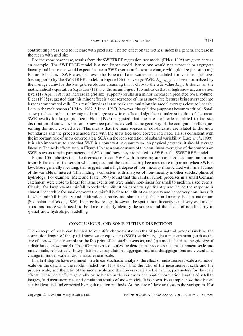
contributing areas tend to increase with pixel size. The net e�ect on the wetness index is a general increase inthe mean with grid size.

For the snow cover case, results from the SWETREE regression tree model (Elder, 1995) are given here asan example. The SWETREE model is a non-linear model, hence one would not expect it to aggregatelinearly and hence one would expect the mean SWE over a catchment to change with grid size (i.e. support).Figure 10b shows SWE averaged over the Emerald Lake watershed calculated for various grid sizes(i.e. supports) by the SWETREE model. In Figure 10b the average SWE, Eapp;Supp, has been normalized bythe average value for the 5 m grid resolution assuming this is close to the true value Etrue . E stands for themathematical expectation (equation (11)), i.e. the mean. Figure 10b indicates that at high snow accumulationlevels (17 April, 1987) an increase in grid size (support) results in a minor increase in predicted SWE volume.Elder (1995) suggested that this minor e�ect is a consequence of linear snow free features being averaged intolarger snow covered cells. This result implies that at peak accumulation the model averages close to linearly.Late in the melt season (21 May, 1987; 5 June, 1987), however, the grid size (support) becomes critical. Smallsnow patches are lost to averaging into large snow free cells and signi®cant underestimation of the meanSWE results for large grid sizes. Elder (1995) suggested that the e�ect of scale is related to the sizedistribution of snow covered and snow free patches, as well as the geometry of the contiguous cells repre-senting the snow covered area. This means that the main sources of non-linearity are related to the snowboundaries and the processes associated with the snow free/snow covered interface. This is consistent withthe important role of snow covered area (SCA) in the representation of subgrid variability (Luce et al., 1999).It is also important to note that SWE is a conservative quantity so, on physical grounds, it should averagelinearly. The scale e�ects seen in Figure 10b are a consequence of the non-linear averaging of the controls onSWE, such as terrain parameters and SCA, and how they are related to SWE in the SWETREE model.

Figure 10b indicates that the decrease of mean SWE with increasing support becomes more importanttowards the end of the season which implies that the non-linearity becomes more important when SWE islow. More generally speaking, this suggests that a high degree of non-linearity is associated with small valuesof the variable of interest. This ®nding is consistent with analyses of non-linearity in other subdisciplines ofhydrology. For example, Merz and Plate (1997) found that the rainfall runo� processes in a small Germancatchment were close to linear for large events but were highly non-linear for small to medium sized events.Clearly, for large events rainfall exceeds the in®ltration capacity signi®cantly and hence the response isalmost linear while for smaller events the rainfall is close to in®ltration capacity and hence very non-linear. Itis when rainfall intensity and in®ltration capacity are similar that the non-linearity is at a maximum(Sivapalan and Wood, 1986). In snow hydrology, however, the spatial non-linearity is not very well under-stood and more work needs to be done to clearly identify the sources and the e�ects of non-linearity inspatial snow hydrologic modelling.

CONCLUSIONS AND SOME FUTURE DIRECTIONS

The concept of scale can be used to quantify characteristic lengths of (a) a natural process (such as thecorrelation length of the spatial snow water equivalent (SWE) variability); (b) a measurement (such as thesize of a snow density sample or the footprint of the satellite sensor), and (c) a model (such as the grid size ofa distributed snow model). The di�erent types of scales are denoted as process scale, measurement scale andmodel scale, respectively. Interpolations, extrapolations, aggregations, and disaggregations are viewed as achange in model scale and/or measurement scale.

In a ®rst step we have examined, in a linear stochastic analysis, the e�ect of measurement scale and modelscale on the data and the model predictions. It is shown that the ratio of the measurement scale and theprocess scale, and the ratio of the model scale and the process scale are the driving parameters for the scalee�ects. These scale e�ects generally cause biases in the variances and spatial correlation lengths of satelliteimages, ®eld measurements, and simulation results of snowmodels. It is shown, by example, how these biasescan be identi®ed and corrected by regularization methods. At the core of these analyses is the variogram. For



the case of snow cover patterns, it is shown that it may be di�cult to infer the true snow cover variabilityfrom the variograms, particularly when they span many orders of magnitude. Speci®cally, it may be di�cultto infer preferred scales and stationarity but for practical applications, local stationarity may be a perfectlyadequate assumption.

In a second step we have examined distributed snow models which are a non-linear deterministic approachto changing the scale. Unlike in the linear case, in these models a change of scale may also bias the mean overa catchment of snow-related variables such as SWE. There are a number of fundamental scaling issues withdistributed models which include subgrid variability, the question of an optimum element size, andparameter identi®ability. We give methods for estimating subgrid variability and point to potential avenuesfor parameterizing subgrid variability. We suggest that, in general, an optimum element size may not existand that the model element scale may in practice be dictated by practical considerations such as dataavailability and the required resolution of the predictions. Model parameters may be more easily identi®ed inspatial index approaches than in distributed physically based snow models but this is at the cost of requiringan extensive data set for proper calibration. The scale e�ects in distributed non-linear models can be relatedto the linear stochastic case. The biases in the mean caused by scale e�ects only occur in the non-linear caseas they are a consequence of the non-linearity present in the natural system and/or the models. However, thereduction in variance with increasing element size (i.e. support) is similar to the linear case which gives somecredence to generalizing the applicability of regularization methods, as an approximation, to non-linearcases.

It is likely that a number of areas of scale related research in snow hydrology will receive particularattention in the near future. The capabilities of obtaining spatial data sets of snow hydrologic quantities havebeen increased manifold in the past years through both satellite imagery and ground based networks (such asthe US SNOTEL network; NRCS, 1998). There exist a number of outstanding data sets such as the snowdepth transect data obtained by a sled mounted X-band FW-CW radar in the Kuparuk Basin in Alaska(Holmgren et al., 1998) and in Antarctica (Sturm et al., 1998). However, it is clear that this trend needs tocontinue. It is the patterns of variables related to snow processes that are likely to best advance theunderstanding of scaling e�ects in snow hydrology. Along with better information on the spatial patterns,there is a need for improved formal methods for assessing spatially distributed snow models based on spatialdata. Work is progressing in this direction in various areas of hydrology (e.g. Western et al., 1996). Suchformal methods may be based on a range of statistical approaches including pattern recognition methods.

If we assume that random behaviour and linear aggregation of snow hydrologic variables apply, there area range of methods available to assess scale e�ects and to perform interpolations, extrapolations, aggrega-tions, and disaggregations in a consistent way. For the non-linear case this is vastly more di�cult and hencemost of the methods addressing the non-linear case are more ad hoc. It would be useful to extend theframework presented here to non-linear cases in the context of snow hydrology. Little is known about thefeedback e�ects of subgrid variability introduced by the non-linearity of the system and yet they are probablyextremely important in distributed snow models. Other subdisciplines of hydrology, such as subsurfacehydrology, have an excellent track record in quantifying non-linear scale e�ects by stochastic methods in aconsistent way (e.g. Dagan, 1986; Gelhar, 1993). Clearly, in the case of snow hydrology the emphasis of thesemethods needs to be on the spatial organization that is present in the natural snow cover environment.

In this paper we have examined the biases caused by the scale e�ects but of similar importance is thereliability of spatial estimates and how it is a�ected by a change of scale. With geographic informationsystems (GIS) and other spatial estimation methods readily available today, it is easy to interpolate betweendata points but it is much more di�cult to assess how accurate these estimates are. It is, therefore, of greatimportance to assess the uncertainty of spatial estimates and to be explicit about uncertainty whenpresenting results of spatial interpolations, extrapolations, aggregations, and disaggregations. The assess-ment of spatial uncertainty is likely to be an area of increasing interest in snow hydrology in the near future.

While most of this paper has focused on physical snow processes, similar conclusions apply and similarmethods are applicable to chemical and biological processes. Scaling problems may even be more acute for


2172 G. BLOÈ SCHL

chemical and biological processes, as in most applications chemical and biological data tend to be morelimited than data about physical processes.

ACKNOWLEDGEMENTS

I am greatly indebted to many people who have helped shape my own ideas on scale issues, in particularM. Sivapalan, R. Grayson, A. Western, D. Gutknecht, R. Kirnbauer, and H. Kupfersberger. I am especiallygrateful to K. Elder and W. Rosenthal who supplied the TM data, R. Davis who supplied the thin sectiondata, and J. Hardy and R. Davis who supplied the AVHRR data. R. Merz assisted in the variogram analysesand G. Haidinger assisted with the drawings. I would like to thank K. Elder, R. Merz and two anonymousreviewers for useful comments on the manuscript. A travel award from the United States Army, EuropeanResearch O�ce (grant #R&D 8637-EN-06) is gratefully acknowledged.

REFERENCES

Anderson EA. 1973. National Weather Service river forecast system Ð snow accumulation and ablation model. NOAA Tech. Rep. NWSHYDRO-17, US Dept. of Commerce: Silver Spring, Maryland.

Anderson MP. 1997. Characterization of geological heterogeneity. In International Hydrology Series, Dagan G, Neuman SP (eds);Cambridge University Press: Cambridge: pp. 23±43.

Armstrong M. 1998. Basic Linear Geostatistics. Springer: Berlin.Band LE, Moore ID. 1995. Scale: Landscape attributes and geographical information systems. Hydrological Processes 9: 401±422.Bathurst JC, Cooley KR. 1996. Use of the SHE hydrological modelling system to investigate basin response to snowmelt at Reynolds

Creek, Idaho. Journal of Hydrology 175: 181±211.Bear J. 1972. Dynamics of Fluids in Porous Media. American Elsevier: New York: 764 pp.Becker A, BloÈ schl G, Hall A. 1999. Land surface heterogeneity and scaling in hydrology. Journal of Hydrology 217: (special issue).Beckie R. 1996. Measurement scale, network sampling scale, and groundwater model parameters.Water Resources Research 32: 65±76.Beven K. 1989. Changing ideas in hydrology Ð the case of physically based models. Journal of Hydrology 105: 157±172.Beven KJ 1995. Linking parameters across scales: Subgrid parameterizations and scale dependent hydrological models. Hydrological

Processes 9: 507±525.BloÈ schl G. 1996. Prozeûnahe Niederschlag-Ab¯uûmodellierung (Process-oriented rainfall-runo� modelling). OÈsterreichische Wasser-

und Abfallwirtschaft 48: 156±165.BloÈ schl G. 1999. Scale and Scaling in Hydrology Ð a Framework for Thinking and Analysis, in press. John Wiley & Sons, Ltd:

Chichester.BloÈ schl G, Kirnbauer R. 1991. Point snowmelt models with di�erent degrees of complexity Ð internal processes. Journal of Hydrology

129: 127±147.BloÈ schl G, Kirnbauer R. 1992. An analysis of snow cover patterns in a small Alpine catchment. Hydrological Processes 6: 99±109.BloÈ schl G, Sivapalan M. 1995. Scale issues in hydrological modelling Ð a review. Hydrological Processes 9: 251±290.BloÈ schl G, Sivapalan M. 1997. Process controls on regional ¯ood frequency: coe�cient of variation and basin scale. Water Resources

Research 33: 2967±2980.BloÈ schl G, Kirnbauer R, Gutknecht D. 1991. Distributed snowmelt simulations in an Alpine catchment. 1. Model evaluation on the

basis of snow cover patterns. Water Resources Research 27: 3171±3179.BloÈ schl G, Gutknecht D, Grayson RB, Sivapalan M, Moore ID. 1993. Organisation and randomness in catchments and the veri®cation

of hydrologic models. EOS, Transactions of the American Geophysical Union 74, 317.BloÈ schl G, Gutknecht D, Kirnbauer R. 1994. On the evaluation of distributed hydrologic models. In Advances in Distributed

Hydrology, Rosso R, Peano A, Becchi I, Bemporad GA (eds); Water Resources Publications: Highlands Ranch, Colorado: 397±412.BloÈ schl G, Grayson RB, Sivapalan M. 1995. On the representative elementary area (REA) concept and its utility for distributed

rainfall-runo� modelling. Hydrological Processes 9: 313±330.BloÈ schl G, Sivapalan M, Gupta VK, Beven K, Lettenmaier D (eds); 1997. Special section on scale problems in hydrology. Water

Resources Research 33(12): 2881±2999.Braun LN. 1985. Simulation of Snowmelt-Runo� in Lowland and Lower Alpine Regions of Switzerland, ZuÈ rcher Geographische Schriften

21. Geographisches Institut der ETH ZuÈ rich: 166 pp.Charbonneau R, Lardeau JP, Obled Ch. 1981. Problems of modelling a high mountainous drainage basin with predominant snow

yields. Hydrological Science Bulletin 26: 345±361.Cline DW, Bales RC, Dozier J. 1998a. Estimating the spatial distribution of snow in mountain basins using remote sensing and energy

balance modeling. Water Resources Research 34: 1275±1285.Cline DW, Elder K, Bales RC. 1998b. Scale e�ects in a distributed snow water equivalence and snowmelt model for mountain basins.

Hydrological Processes 12: 1527±1536.Cushman JH. 1984. Unifying the concepts of scale, instrumentation, and stochastics in the development of multiphase transport

theory. Water Resources Research 20: 1668±1676.Cushman JH. 1987. More on stochastic models. Water ResourcesResearch 23: 750±752.



Dagan G. 1986. Statistical theory of groundwater ¯ow and transport: Pore to laboratory, laboratory to formation and formation toregional scale. Water Resources Research 22: 120S±134S.

Davis RE, McKenzie JC, Jordan R. 1995. Distributed snow process modelling: an image processing approach. Hydrological Processes9: 865±875.

Deutsch CV, Journel AG. 1997. GSLIB, Geostatistical Software Library and User's Guide. Oxford University Press: New York:384 pp.

Dozier J. 1980. A clear-sky spectral solar radiation model for snow-covered mountainous terrain. Water Resources Research 16:709±718.

Elder K. 1995. Snow distribution in alpine watersheds. Ph.D. dissertation: University of California, Santa Barbara, 309 pp.Elder K, Dozier J, Michaelsen J. 1989. Spatial and temporal variation of net snow accumulation in a small alpine watershed, Emerald

Lake basin, Sierra Nevada, California, USA.. Annals of Glaciology 13: 56±63.Famiglietti JS. 1992. Aggregation and scaling of spatially-variable hydrological processes: Local, catchment-scale and macroscale models

of water and energy balance. Ph.D. dissertation: Princeton University, 207 pp.Fan Y, Bras RL. 1995. On the concept of a representative elementary area in catchment runo�. Hydrological Processes 9: 821±832.Feder J. 1988. Fractals, Plenum: New York and London: 283 pp.Federico VD, Neuman SP. 1997. Scaling of random ®elds by means of truncated power variograms and associated spectra. Water

Resources Research 33: 1075±1085.Foufoula-Georgiou E, Sapozhnikov VB. 1998. Anisotropic scaling in braided rivers: An integrated theoretical framework and results

from application to an experimental river. Water Resources Research 34: 863±867.Gallant JC, Moore ID, Hutchinson MF, Gessler PE. 1994. Estimating fractal dimension of pro®les: a comparison of methods.

Mathematical Geology 26: 455±481.Gelhar LW. 1993. Stochastic Subsurface Hydrology, Prentice Hall: Englewood Cli�s, NJ: 390 pp.Golden Software 1998. [online] available: http://golden.com/golden/products/surfer/surfer.htm. Golden Software, Inc., 809 14th Street,

Golden, Colorado 80401-1866, USA.Golding DL. 1974. The correlation of snowpack with topography and snowmelt runo� on Marmot Creek basin, Alberta. Atmosphere

12: 31±38.Goodrich DC, Lane LJ, Shillito RM, Miller SN, Syed KH, Woolhiser DA. 1997. Linearity of basin response as a function of scale in a

semiarid watershed. Water Resources Research 33: 2951±2965.Grayson RB, Moore ID, McMahon TA. 1992. Physically-based hydrologic modelling: 2. Is the concept realistic? Water Resources

Research 26: 2659±2666.Grayson RB, BloÈ schl G, Barling RD, Moore ID. 1993. Process, scale and constraints to hydrological modelling in GIS. In Applications

of Geographic Information Systems in Hydrology and Water Resources Management, Kovar K, Nachtnebel HP (eds), (Proc. ViennaSymp., April 1993). IAHS Publ. No. 211, 83±92.

Grayson RB, BloÈ schl G, Moore ID. 1995. Distributed parameter hydrologic modelling using vector elevation data: THALES andTAPES-C, Chapter 19. In Computer Models of Watershed Hydrology, Singh VP (ed.); Water Resources Publications: HighlandsRanch, Colorado: 669±696.

Gupta VK, RodrõÂ guez-Iturbe I, Wood EF (eds); 1986. Scale Problems in Hydrology. D. Reidel Publ.: Dordrecht, Holland: 246 pp.Holmgren J, Sturm M, Yankielun NE, Koh G. 1998. Extensive measurements of snow depth using FM-CW radar. Cold Regions

Science and Technology 27: 17±30.Houghton JT, Filho LGM, Callander BA, Harris N, Kattenburg A, Maskell K. 1996. Climate Change 1995: The Science of Climate

Change. Cambridge University Press: Cambridge: 584 pp.Hubbert MK. 1956. Darcy's law and the ®eld equations of the ¯ow of underground ¯uids. Transactions of the American Institute of

Mining and Metallurgical Engineers 207: 222±239.Isaaks EH, Srivastava RM. 1989. An Introduction to Applied Geostatistics. Oxford University Press: New York, Oxford: 561 pp.Journel AG, Huijbregts CJ. 1978. Mining Geostatistics, Academic Press: London: 600 pp.Journel AG. 1993. Geostatistics: roadblocks and challenges. In Geostatistics TroÂia '92, Soares A (ed.); Kluwer Academic Publishers:

Dordrecht, The Netherlands: pp. 213±224.Kalma JD, Sivapalan M. (eds); 1995. Scale issues in hydrological modelling. In Advances in Hydrological Processes, John Wiley & Sons,

Ltd: Chichester: 489 pp.Kirnbauer R, BloÈ schl G, Gutknecht D. 1994. Entering the era of distributed snow models. Nordic Hydrology 25: 1±24.KlemesÏ V. 1974. The Hurst phenomenon: A puzzle? Water Resources Research 10: 675±688.Klinkenberg B, Goodchild MF. 1992. The fractal properties of topography: a comparison of methods. Earth Surface Processes and

Landforms 17: 217±234.Kutilek M, Zayani K, Haverkamp R, Parlange JY, Vachaud G. 1991. Scaling of the Richards equation under invariant ¯ux boundary

conditions. Water Resources Research 27: 2181±2185.Leavesley GH 1989. Problems of snowmelt runo� modelling for a variety of physiographic and climatic conditions. Hydrological

Science Journal 34: 617±634.Lever JH, Haehnel R. 1995. Scaling snowdrift development rate. Hydrological Processes 9: 935±946.Loague K. 1990. R-5 Revisited. 2. Reevaluation of a quasi-physically based rainfall-runo� model with supplemental information.

Water Resources Research 26: 973±987.Lovejoy S, Schertzer D. 1985. Generalized scale invariance and fractal models of rain. Water Resources Research 21: 1233±1250.Luce CH, Tarboton DG, Cooley KR. 1999. Subgrid parameterization of snow distribution for an energy and mass balance snow cover

model. Hydrological Processes 13: 1921±1933.Merz B, Plate EJ. 1997. An analysis of the e�ects of spatial variability of soil and soil moisture on runo�.Water Resources Research 33:

2909±2922.


2174 G. BLOÈ SCHL

Michaud JD, Shuttleworth WJ. 1997. Aggregate description of land-atmosphere interactions. Journal of Hydrology 190: (special issue).Moore ID, Grayson RB, Ladson AR. 1991. Digital terrain modelling: A review of hydrological, geomorphological, and biological

applications. Hydrological Processes 5: 3±30.Neuman SP. 1990. Universal scaling of hydraulic conductivities and dispersivities in geologic media. Water Resources Research 26:

1749±1758.Neuman SP 1993. Comment on À critical review of data on ®eld-scale dispersion in aquifers' by L. W. Gelhar, C. Welty, and K. R.

Rehfeldt. Water Resources Research 29: 1863±1865.NRCS 1998. [online] available: http://www.wcc.nrcs.usda.gov/. Snow Survey and Water Supply Forecasting Program Manager,

Natural Resources Conservation Service, 101 SW Main Street, Suite 1600, Portland, Oregon 97204-3224, USA.Obled Ch. 1990. Hydrological modeling in regions of rugged relief. In Hydrology in Mountainous Regions. I Ð Hydrological Measure-

ments; the Water Cycle, Lang H, Musy A (eds); Proc. Lausanne Symp., Aug. 1990. IAHS Publ. 193. pp. 599±613.Obled Ch, Harder H. 1979. A review of snow melt in the mountain environment. In Modeling of Snow Cover Runo�, Colbeck SC,

Ray M (eds); Proc. Meeting, Hanover, New Hampshire, Sept. 1978: US Army Cold Regions Research and Engineering Laboratory.pp. 179±204.

RodrõÂ guez-Iturbe I, Gupta VK. (eds); 1983. Scale problems in hydrology. Journal of Hydrology 65: (special issue).RodrõÂ guez-Iturbe I, MejõÂ a JM. 1974. On the transformation from point rainfall to areal rainfall.Water Resources Research 10: 729±735.Rosenthal W, Dozier J. 1996. Automated mapping of montane snow cover at subpixel resolution from the Landsat Thematic Mapper.

Water Resources Research 32: 115±130.Russo D, Jury WA. 1987. A theoretical study of the estimation of the correlation scale in spatially variable ®elds. 1. Stationary ®elds.

Water Resources Research 23: 1257±1268.Seyfried MS, Wilcox BP. 1995. Scale and the nature of spatial variability: ®eld examples having implications for hydrologic modeling.

Water Resources Research 31: 173±184.Sivapalan M, BloÈ schl G. 1998. Transformation of point rainfall to areal rainfall: intensity-duration-frequency curves. Journal of

Hydrology 204: 150±167.Sivapalan M, Wood EF. 1986. Spatial heterogeneity and scale in the in®ltration response of catchments. In Scale Problems in

Hydrology, Gupta VK, RodrõÂ guez-Iturbe I, Wood EF (eds); D. Reidel Publ.: Dordrecht, Holland: 81±106.Smagorinsky J. 1974. Global atmospheric modeling and the numerical simulation of climate. In Weather and Climate Modi®cation,

Hess WN (ed.); John Wiley & Sons, Ltd: New York: 633±686.Sommerfeld RA, Bales RC. 1993. Spatial statistics of snowmelt from lysimeters and aerial photos. EOS, Transactions of the American

Geophysical Union 74: 247.Shook K, Gray DM 1996. Small-scale spatial structure of shallow snowcovers. Hydrological Processes 10: 1283±1292.Sturm M, Morris K, Massom R. 1998. The winter snow cover of the West Antarctic pack ice: its spatial and temporal variability. In

Antarctic Sea Ice Ð Antarctic Research Series 74, Je�ries M. O. (ed.); American Geophysical Union: Washington, D.C.: 1±18.Tarboton DG, Luce CH. 1996. Utah Energy Balance Snow Accumulation and Melt Model (UEB), Computer model technical

description and users guide: Utah Water Research Laboratory and USDA Forest Service Intermountain Research Station.Vanmarcke E. 1983. Random Fields: Analysis and Synthesis, The MIT Press: Cambridge, Massachusetts: 382 pp.Wen X-H, GoÂ mez-HernaÂ ndez JJ. 1996. Upscaling hydraulic conductivities in heterogeneous media: An overview. Journal of Hydrology

183: ix±xxxii.Western AW, BloÈ schl G. 1999. On the spatial scaling of soil moisture. Journal of Hydrology 217: 203±224.Western AW, BloÈ schl G, Willgoose GR, Grayson RB, McMahon TA. 1996. Comparison of measured and predicted soil moisture

patterns. EOS, Transactions of the American Geophysical Union 77(22); w34.Western AW, BloÈ schl G, Grayson RB. 1998. How well do indicator variograms capture the spatial connectivity of soil moisture?

Hydrological Processes 12: 1851±1868.Wiener N. 1966. Extrapolation, Interpolation and Smoothing of Stationary Time Series, The MIT Press: Cambridge, Mass: 163 pp.Wood EF, Sivapalan M., Beven, K, Band L. 1988. E�ects of spatial variability and scale with implications to hydrologic modeling.

Journal of Hydrology 102: 29±47.World Meteorological Organisation 1986. Intercomparison of models of snowmelt runo�. Operational Hydrology Report no. 23,

Publication no. 646, World Meteorological Organisation: Geneva.Yang D, Woo MK. 1999. Representativeness of local snow data for large scale hydrologic investigations in the Arctic. Hydrological

Processes 13: 1977±1988.



Documents

Scaling issues in snow hydrology - University of Washingtondepts.washington.edu/mtnhydr/snowschool/Bloschl1999.pdfIn a second step we examine distributed snow models which are a non-linear