Embed Size (px)
Citation preview
Some Recent Advances in Alternating DirectionMethods: Practice and Theory
Yin Zhang (张寅)
Department of Computational and Applied MathematicsRice University, Houston, Texas, USA
The 5th Sino-Japanese Optimization Meeting
Beijing, China, September 28, 2011
Outline:
Alternating Direction Method (ADM)
Recent Revival and Extensions
Local Convergence and Rate
Global Convergence
Summary
Contributors:Xin Liu, Junfeng Yang, Zaiwen Wen, Yilun Wang, Chengbo Li,Yuan Shen, Wei Deng, Wotao Yin
, 2/39
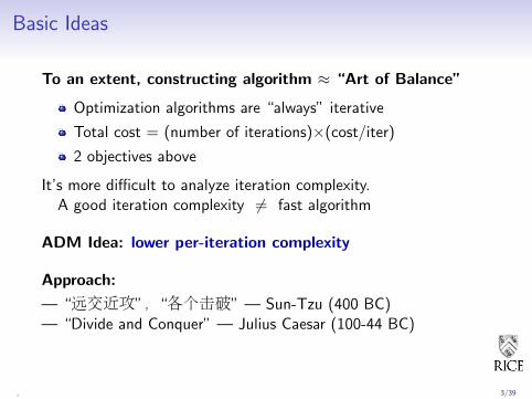
Basic Ideas
To an extent, constructing algorithm ≈ “Art of Balance”
Optimization algorithms are “always” iterative
Total cost = (number of iterations)×(cost/iter)
2 objectives above
It’s more difficult to analyze iteration complexity.A good iteration complexity 6= fast algorithm
ADM Idea: lower per-iteration complexity
Approach:
— “远交近攻”,“各个击破” — Sun-Tzu (400 BC)— “Divide and Conquer” — Julius Caesar (100-44 BC)
, 3/39
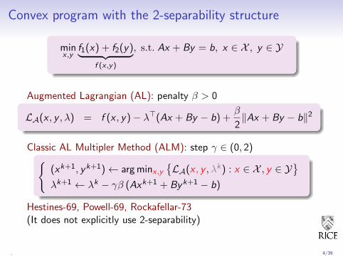
Convex program with the 2-separability structure
minx ,y
f1(x) + f2(y)︸ ︷︷ ︸f (x ,y)
, s.t. Ax + By = b, x ∈ X , y ∈ Y
Augmented Lagrangian (AL): penalty β > 0
LA(x , y , λ) = f (x , y)− λ>(Ax + By − b) +β
2‖Ax + By − b‖2
Classic AL Multipler Method (ALM): step γ ∈ (0, 2)(xk+1, yk+1)← arg minx ,y
LA(x , y , λk ) : x ∈ X , y ∈ Y
λk+1 ← λk − γβ (Axk+1 + Byk+1 − b)
Hestines-69, Powell-69, Rockafellar-73(It does not explicitly use 2-separability)
, 4/39
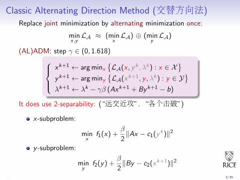
Classic Alternating Direction Method (交替方向法)
Replace joint minimization by alternating minimization once:
minx ,yLA ≈ (min
xLA) ⊕ (min
yLA)
(AL)ADM: step γ ∈ (0, 1.618)xk+1 ← arg minx
LA(x , yk , λk ) : x ∈ X
yk+1 ← arg miny
LA(xk+1, y , λk ) : y ∈ Y
λk+1 ← λk − γβ (Axk+1 + Byk+1 − b)
It does use 2-separability: (“远交近攻”,“各个击破”)
x-subproblem:
minx
f1(x) +β
2‖Ax − c1(yk )‖2
y -subproblem:
miny
f2(y) +β
2‖By − c2(xk+1)‖2
, 5/39
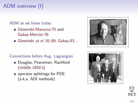
ADM overview (I)
ADM as we know today
Glowinski-Marocco-75 andGabay-Mercier-76
Glowinski at el. 81-89, Gabay-83...
Connections before Aug. Lagrangian
Douglas, Peaceman, Rachford(middle 1950’s)
operator splittings for PDE(a.k.a. ADI methods)
, 6/39

ADM overview (II)
After PDE, subsequent studies in optimization
variational inequality, proximal-point, Bregman, ...(Eckstein-Bertsekas-92 ......)
inexact ADM (He-Liao-Han-Yang-02 ......)
Tseng-91, Fukushima-92, ...
proximal-like, Bregman (Chen and Teboulle-93)
......
ADM had been used in optimization to some extent, but notas widely used to be called “main-stream” algorithm
, 7/39

ADM overview (III)
Recent Revival in Signal/Image/Data Processing
`1-norm, total variation (TV) minimization
convex, non-smooth, simple structures
Splitting + alternating:
Wang-Yang-Yin-Z-2008, FTVd (TV code)(split + quadratic penalty, 2007)(split + quadratic penalty + multiplier in code, 2008)
Goldstein-Osher-2008, split Bregman(split + quadratic penalty + Bregman, earlier in 2008)
ADM `1-solver for 8 models: YALL1. Yang-Z-2010
Googled “split Bregman”: “found 16,300 results”.Turns out that hot split Bregman = cool ALM
, 8/39
ADM Global Convergence
e.g., “Augmented Lagrangian methods ...” Fortin-Glowinski-83
Assumptions required by current theory:
convexity over the entire domain
separability for exactly 2 blocks, no more
exact or high-accuracy minimization for each block
Strength:
differentiability not required
side-constraints allowed: x ∈ X , y ∈ Y
But
why not 3 or more blocks?
very rough minimization?
rate of convergence?
, 9/39
Some Recent Applications
From PDE to:
Signal/Image Processing
Sparse Optimization
, 10/39
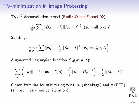
TV-minimization in Image Processing
TV/L2 deconvolution model (Rudin-Osher-Fatemi-92):
minu
∑i‖Diu‖+
µ
2‖Ku − f ‖2 (sum all pixels)
Splitting:
minu,w
∑‖wi‖+
µ
2‖Ku − f ‖2 : wi = Diu,∀i
.
Augmented Lagrangian function LA(w, u, λ):∑i
(‖wi‖ − λ>i (wi − Diu) +
β
2‖wi − Diu‖2
)+µ
2‖Ku − f ‖2.
Closed formulas for minimizing w.r.t. w (shrinkage) and u (FFT)(almost linear-time per iteration)
, 11/39
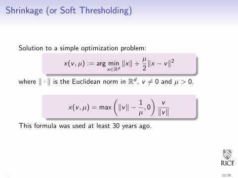
Shrinkage (or Soft Thresholding)
Solution to a simple optimization problem:
x(v , µ) := arg minx∈Rd
‖x‖+µ
2‖x − v‖2
where ‖ · ‖ is the Euclidean norm in Rd , v 6= 0 and µ > 0.
x(v , µ) = max
(‖v‖ − 1
µ, 0
)v
‖v‖
This formula was used at least 30 years ago.
, 12/39
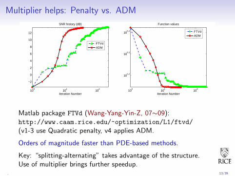
Multiplier helps: Penalty vs. ADM
100
101
102
−2
0
2
4
6
8
10
12
Iteration Number
SNR history (dB)
FTVdADM
100
101
102
105.2
105.3
105.4
Iteration Number
Function values
FTVdADM
Matlab package FTVd (Wang-Yang-Yin-Z, 07∼09):http://www.caam.rice.edu/~optimization/L1/ftvd/
(v1-3 use Quadratic penalty, v4 applies ADM.
Orders of magnitude faster than PDE-based methods.
Key: “splitting-alternating” takes advantage of the structure.Use of multiplier brings further speedup.
, 13/39
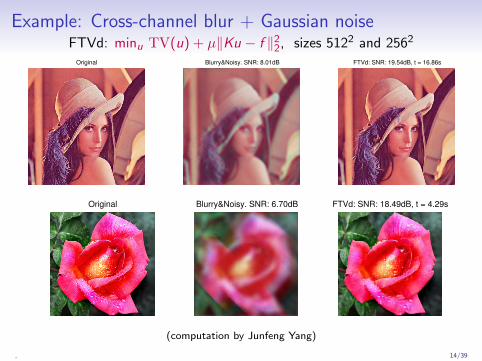
Example: Cross-channel blur + Gaussian noiseFTVd: minu TV(u) + µ‖Ku − f ‖2
2, sizes 5122 and 2562
Original Blurry&Noisy. SNR: 8.01dB FTVd: SNR: 19.54dB, t = 16.86s
Original Blurry&Noisy. SNR: 6.70dB FTVd: SNR: 18.49dB, t = 4.29s
(computation by Junfeng Yang)
, 14/39
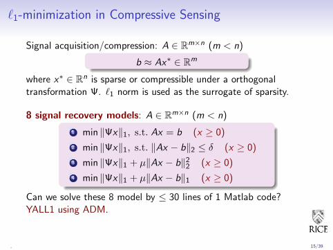
`1-minimization in Compressive Sensing
Signal acquisition/compression: A ∈ Rm×n (m < n)
b ≈ Ax∗ ∈ Rm
where x∗ ∈ Rn is sparse or compressible under a orthogonaltransformation Ψ. `1 norm is used as the surrogate of sparsity.
8 signal recovery models: A ∈ Rm×n (m < n)
1 min ‖Ψx‖1, s.t. Ax = b (x ≥ 0)
2 min ‖Ψx‖1, s.t. ‖Ax − b‖2 ≤ δ (x ≥ 0)
3 min ‖Ψx‖1 + µ‖Ax − b‖22 (x ≥ 0)
4 min ‖Ψx‖1 + µ‖Ax − b‖1 (x ≥ 0)
Can we solve these 8 model by ≤ 30 lines of 1 Matlab code?YALL1 using ADM.
, 15/39
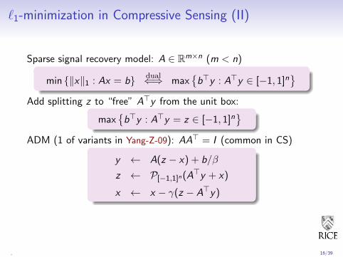
`1-minimization in Compressive Sensing (II)
Sparse signal recovery model: A ∈ Rm×n (m < n)
min ‖x‖1 : Ax = b dual⇐⇒ maxb>y : A>y ∈ [−1, 1]n
Add splitting z to “free” A>y from the unit box:
maxb>y : A>y = z ∈ [−1, 1]n
ADM (1 of variants in Yang-Z-09): AA> = I (common in CS)
y ← A(z − x) + b/β
z ← P[−1,1]n (A>y + x)
x ← x − γ(z − A>y)
, 16/39
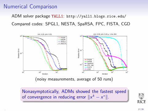
Numerical Comparison
ADM solver package YALL1: http://yall1.blogs.rice.edu/
Compared codes: SPGL1, NESTA, SpaRSA, FPC, FISTA, CGD
100
101
102
10−1
100
Iteration
Rel
ativ
e E
rror
m/n: 0.20, p/m: 0.20,
PADMDADMSPGL1NESTA
100
101
102
103
10−2
10−1
100
Iteration
Rel
ativ
e E
rror
m/n: 0.30, p/m: 0.20, μ: 1.0e−004
PADMDADMSpaRSAFPC_BBFISTACGD
(noisy measurements, average of 50 runs)
Nonasymptotically, ADMs showed the fastest speedof convergence in reducing error ‖xk − x∗‖.
, 17/39
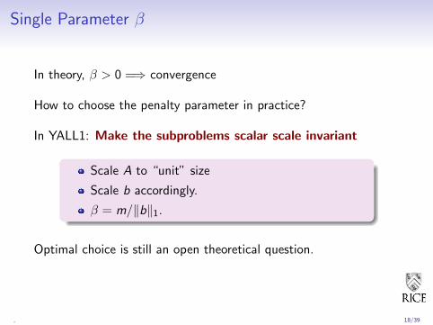
Single Parameter β
In theory, β > 0 =⇒ convergence
How to choose the penalty parameter in practice?
In YALL1: Make the subproblems scalar scale invariant
Scale A to “unit” size
Scale b accordingly.
β = m/‖b‖1.
Optimal choice is still an open theoretical question.
, 18/39
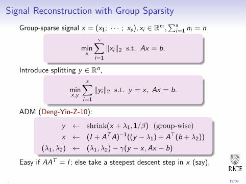
Signal Reconstruction with Group Sparsity
Group-sparse signal x = (x1; · · · ; xs), xi ∈ Rni ,∑s
i=1 ni = n
minx
s∑i=1
‖xi‖2 s.t. Ax = b.
Introduce splitting y ∈ Rn,
minx ,y
s∑i=1
‖yi‖2 s.t. y = x , Ax = b.
ADM (Deng-Yin-Z-10):
y ← shrink(x + λ1, 1/β) (group-wise)
x ← (I + ATA)−1((y − λ1) + A>(b + λ2))
(λ1, λ2) ← (λ1, λ2)− γ(y − x ,Ax − b)
Easy if AAT = I ; else take a steepest descent step in x (say).
, 19/39
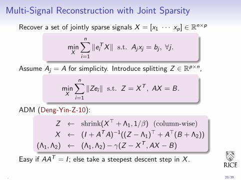
Multi-Signal Reconstruction with Joint Sparsity
Recover a set of jointly sparse signals X = [x1 · · · xp] ∈ Rn×p
minX
n∑i=1
‖eTi X‖ s.t. Ajxj = bj , ∀j .
Assume Aj = A for simplicity. Introduce splitting Z ∈ Rp×n,
minX
n∑i=1
‖Zei‖ s.t. Z = XT , AX = B.
ADM (Deng-Yin-Z-10):
Z ← shrink(X> + Λ1, 1/β) (column-wise)
X ← (I + ATA)−1((Z − Λ1)> + A>(B + Λ2))
(Λ1,Λ2) ← (Λ1,Λ2)− γ(Z − XT ,AX − B)
Easy if AAT = I ; else take a steepest descent step in X .
, 20/39
Extensions to Non-convex Territories
(as long as convexity exists in each direction)
Low-Rank/Sparse Matrix Models
Non-separable functions
More than 2 blocks
, 21/39
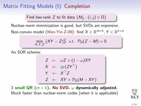
Matrix Fitting Models (I): Completion
Find low-rank Z to fit data Mij : (i , j) ∈ Ω
Nuclear-norm minimization is good, but SVDs are expensive.
Non-convex model (Wen-Yin-Z-09): find X ∈ Rm×k ,Y ∈ Rk×n
minX ,Y ,Z
‖XY − Z‖2F s.t. PΩ(Z −M) = 0
An SOR scheme:
Z ← ωZ + (1− ω)XY
X ← qr(ZY>)
Y ← X>Z
Z ← XY + PΩ(M − XY )
1 small QR (m × k). No SVD. ω dynamically adjusted.Much faster than nuclear-norm codes (when it is applicable)
, 22/39
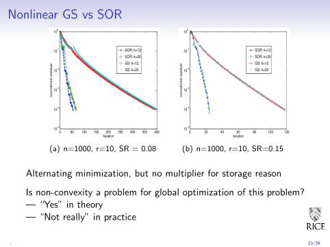
Nonlinear GS vs SOR
0 50 100 150 200 250 300 350 40010
−5
10−4
10−3
10−2
10−1
100
iteration
no
rm
alize
d r
esid
ua
l
SOR: k=12
SOR: k=20
GS: k=12
GS: k=20
(a) n=1000, r=10, SR = 0.08
0 20 40 60 80 100 12010
−5
10−4
10−3
10−2
10−1
100
iteration
no
rm
alize
d r
esid
ua
l
SOR: k=12
SOR: k=20
GS: k=12
GS: k=20
(b) n=1000, r=10, SR=0.15
Alternating minimization, but no multiplier for storage reason
Is non-convexity a problem for global optimization of this problem?— “Yes” in theory— “Not really” in practice
, 23/39
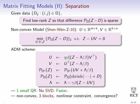
Matrix Fitting Models (II): SeparationGiven data Dij : (i , j) ∈ Ω,
Find low-rank Z so that difference PΩ(Z−D) is sparse
Non-convex Model (Shen-Wen-Z-10): U ∈ Rm×k ,V ∈ Rk×n
minU,V ,Z
‖PΩ(Z − D)‖1 s.t. Z − UV = 0
ADM scheme:
U ← qr((Z − Λ/β)V>)
V ← U>(Z − Λ/β)
PΩc (Z ) ← PΩc (UV + Λ/β)
PΩ(Z ) ← PΩ(shrink(· · · ) + D)
Λ ← Λ− γβ(Z − UV )
— 1 small QR. No SVD. Faster.— non-convex, 3 blocks. nonlinear constraint. convergence?
, 24/39
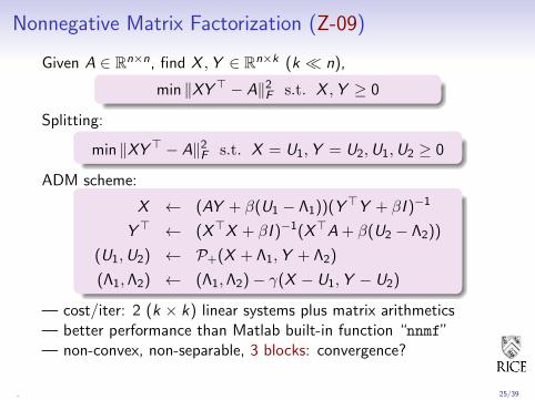
Nonnegative Matrix Factorization (Z-09)
Given A ∈ Rn×n, find X ,Y ∈ Rn×k (k n),
min ‖XY> − A‖2F s.t. X ,Y ≥ 0
Splitting:
min ‖XY> − A‖2F s.t. X = U1,Y = U2,U1,U2 ≥ 0
ADM scheme:
X ← (AY + β(U1 − Λ1))(Y>Y + βI )−1
Y> ← (X>X + βI )−1(X>A + β(U2 − Λ2))
(U1,U2) ← P+(X + Λ1,Y + Λ2)
(Λ1,Λ2) ← (Λ1,Λ2)− γ(X − U1,Y − U2)
— cost/iter: 2 (k × k) linear systems plus matrix arithmetics— better performance than Matlab built-in function “nnmf”— non-convex, non-separable, 3 blocks: convergence?
, 25/39

Theoretical Convergence Results
A general setting
Local R-linear convergence
Global convergence for linear constraints
(Liu-Yang-Z, work in progress)
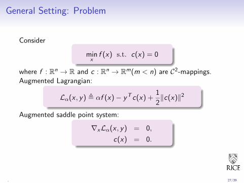
General Setting: Problem
Consider
minx
f (x) s.t. c(x) = 0
where f : Rn → R and c : Rn → Rm(m < n) are C2-mappings.Augmented Lagrangian:
Lα(x , y) , αf (x)− yT c(x) +1
2‖c(x)‖2
Augmented saddle point system:
∇xLα(x , y) = 0,
c(x) = 0.
, 27/39
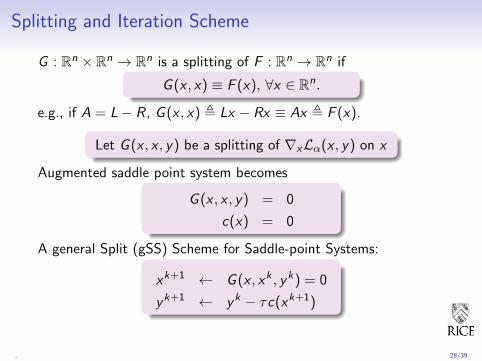
Splitting and Iteration Scheme
G : Rn × Rn → Rn is a splitting of F : Rn → Rn if
G (x , x) ≡ F (x), ∀x ∈ Rn.
e.g., if A = L− R, G (x , x) , Lx − Rx ≡ Ax , F (x).
Let G (x , x , y) be a splitting of ∇xLα(x , y) on x
Augmented saddle point system becomes
G (x , x , y) = 0
c(x) = 0
A general Split (gSS) Scheme for Saddle-point Systems:
xk+1 ← G (x , xk , yk ) = 0
yk+1 ← yk − τc(xk+1)
, 28/39
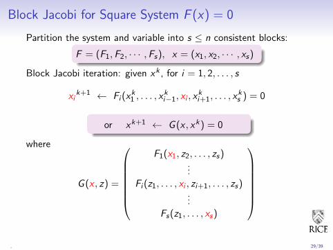
Block Jacobi for Square System F (x) = 0
Partition the system and variable into s ≤ n consistent blocks:
F = (F1,F2, · · · ,Fs), x = (x1, x2, · · · , xs)
Block Jacobi iteration: given xk , for i = 1, 2, . . . , s
xik+1 ← Fi (x
k1 , . . . , x
ki−1, xi , x
ki+1, . . . , x
ks ) = 0
or xk+1 ← G (x , xk ) = 0
where
G (x , z) =
F1(x1, z2, . . . , zs)
...Fi (z1, . . . , xi , zi+1, . . . , zs)
...Fs(z1, . . . , xs)
, 29/39
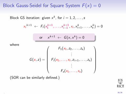
Block Gauss-Seidel for Square System F (x) = 0
Block GS iteration: given xk , for i = 1, 2, . . . , s
xik+1 ← Fi (x
k+11 , . . . , xk+1
i−1 , xi , xki+1, . . . , x
ks ) = 0
or xk+1 ← G (x , xk ) = 0
where
G (x , z) =
F1(x1, z2, . . . , zs)
...Fi (x1, . . . , xi , zi+1, . . . , zs)
...Fs(x1, . . . , xs)
(SOR can be similarly defined.)
, 30/39
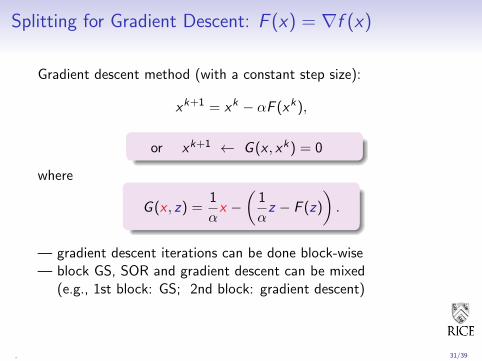
Splitting for Gradient Descent: F (x) = ∇f (x)
Gradient descent method (with a constant step size):
xk+1 = xk − αF (xk ),
or xk+1 ← G (x , xk ) = 0
where
G (x , z) =1
αx −
(1
αz − F (z)
).
— gradient descent iterations can be done block-wise— block GS, SOR and gradient descent can be mixed
(e.g., 1st block: GS; 2nd block: gradient descent)
, 31/39
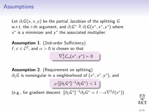
Assumptions
Let ∂iG (x , x , y) be the partial Jacobian of the splitting Gw.r.t. the i-th argument, and ∂iG
∗ , ∂iG (x∗, x∗, y∗) wherex∗ is a minimizer and y∗ the associated multiplier.
Assumption 1. (2nd-order Sufficiency)f , c ∈ C2, and α > 0 is chosen so that
∇2xLα(x∗, y∗) 0
Assumption 2. (Requirement on splitting)∂1G is nonsingular in a neighborhood of (x∗, x∗, y∗), and
ρ([∂1G
∗]−1∂2G∗) < 1
(e.g., for gradient descent: [∂1G∗]−1∂2G
∗ = I − α∇2f (x∗))
, 32/39

Assumptions are Reasonable
A1. 2nd-order sufficiency guarantees that α > 0 exists so that
α[∇2f (x∗)−
∑i y∗i ∇2ci (x
∗)]
+ A(x∗)>A(x∗) 0
where A(x) = ∂c(x). Note
∇xLα(x , y) = G (x , x , y) =⇒ ∇2xL∗α = ∂1G
∗ + ∂2G∗ 0
A2. Any convergent linear splitting for matrices 0 leads to acorresponding nonlinear splitting G satisfying
ρ([∂1G
∗]−1∂2G∗) < 1
Hence, A2 is satisfied by block GS (i.e., ADM), SOR, gradientdescent (with appropriate α) and their mixtures.
, 33/39
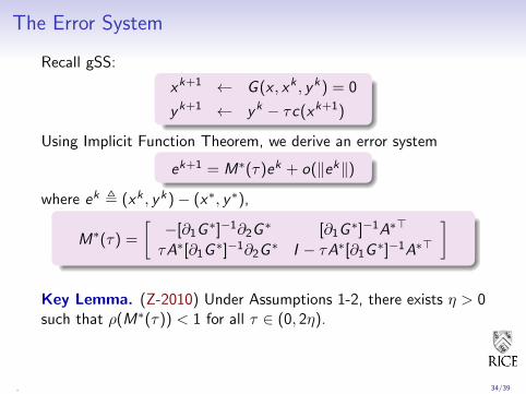
The Error System
Recall gSS:
xk+1 ← G (x , xk , yk ) = 0
yk+1 ← yk − τc(xk+1)
Using Implicit Function Theorem, we derive an error system
ek+1 = M∗(τ)ek + o(‖ek‖)
where ek , (xk , yk )− (x∗, y∗),
M∗(τ) =
[−[∂1G
∗]−1∂2G∗ [∂1G
∗]−1A∗>
τA∗[∂1G∗]−1∂2G
∗ I − τA∗[∂1G∗]−1A∗>
]
Key Lemma. (Z-2010) Under Assumptions 1-2, there exists η > 0such that ρ(M∗(τ)) < 1 for all τ ∈ (0, 2η).
, 34/39
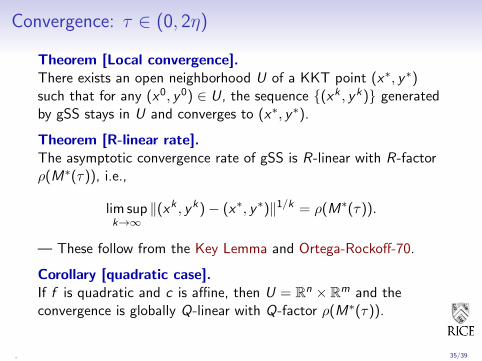
Convergence: τ ∈ (0, 2η)
Theorem [Local convergence].There exists an open neighborhood U of a KKT point (x∗, y∗)such that for any (x0, y0) ∈ U, the sequence (xk , yk ) generatedby gSS stays in U and converges to (x∗, y∗).
Theorem [R-linear rate].The asymptotic convergence rate of gSS is R-linear with R-factorρ(M∗(τ)), i.e.,
lim supk→∞
‖(xk , yk )− (x∗, y∗)‖1/k = ρ(M∗(τ)).
— These follow from the Key Lemma and Ortega-Rockoff-70.
Corollary [quadratic case].If f is quadratic and c is affine, then U = Rn × Rm and theconvergence is globally Q-linear with Q-factor ρ(M∗(τ)).
, 35/39

Global Convergence: Linear Constraints
minx
f (x1, · · · , xp), s.t.∑
Aixi = b
1st-order optimality or saddle point system:
∇f (x) = A>y
Ax − b = 0
Augmented saddle point system:
∇f (x) + βA>(Ax − b) = A>y
y − τβ(Ax − b) = y
Splittings (F (x) = G (x , x)) can be applied to the 1st equation.
Block Jacobi type give block diagonal split
ADM: a block Gauss-Seidel type split
, 36/39
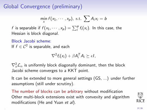
Global Convergence (preliminary)
minx
f (x1, · · · , xp), s.t.∑
Aixi = b
f is separable if f (x1, · · · , xp) =∑p
i fi (xi ). In this case, theHessian is block diagonal.
Block Jacobi scheme:If f ∈ C2 is separable, and each
∇2fi (xi ) + βATi Ai εI ,
∇2xLα is uniformly block diagonally dominant, then the block
Jacobi scheme converges to a KKT point.
It can be extended to more general settings (GS, ...) under furtherassumptions (still under scrutiny).
The number of blocks can be arbitrary without modificationOther multi-block extensions exist with convexity and algorithmmodifications (He and Yuan et al).
, 37/39
Summary: ADM ' Splitting + Alternating
A simple yet effective approach to exploiting structures:
bypasses non-differentiability
enables very cheap iterations
has at least an R-linear rate
great versatility, good efficiency
Many issues remain. Convergence theory needs more work.
, 38/39
References on Codes
(FISTA) A. Beck, and M. Teboulle, “A Fast Iterative Shrinkage-ThresholdingAlgorithm for Linear Inverse Problems”, SIAM J. Imag. Sci., 2:183-202, 2009.
(NESTA) J. Bobin, S. Becker, and E. Candes, “NESTA: A Fast and AccurateFirst-order Method for Sparse Recovery”, TR, CalTech, April 2009.
(SPGL1) M. P. Friedlander and E. van den Berg, “Probing the Pareto frontierfor basis pursuit solutions”, SIAM J. Sci. Comput., 31(2):890–912, 2008.
(FPC) E. T. Hale, W. Yin, and Y. Zhang, “Fixed-point continuation forl1-minimization: Methodology and convergence”, SIAM J. Optim,19(3):1107–1130, 2008.
(IALM) Z. Lin, M. Chen, L. Wu, and Y. Ma, “The Augmented LagrangeMultiplier Method for Exact Recovery of Corrupted Low-Rank Matrices”, TRUIUC, UILU-ENG-09-2215, Nov. 2009.
(FPCA) S. Ma, D. Goldfarb and L. Chen, “Fixed Point and Bregman IterativeMethods for Matrix Rank Minimization”, Math. Prog., to appear.
(APGL) K.-C. Toh, and S. W. Yun, “An accelerated proximal gradient algorithmfor nuclear norm regularized least squares problems”, Pacific J. Optimization.
(SpaRSA) S. Wright, R. Nowak, M. Figueiredo, “Sparse reconstruction byseparable approximation”, IEEE Trans Signal Process., 57(7):2479–2493, 2009.
(CGD) S. Yun, and K.-C. Toh, “A coordinate gradient descent method forL1-regularized convex minimization”, Computational Optimization andApplications, to appear.
, 39/39