Embed Size (px)
Citation preview
Signifikan: Jurnal Ilmu Ekonomi
Volume 6 (2), October 2017
P-ISSN: 2087-2046; E-ISSN: 2476-9223
Page 217 – 230
http://journal.uinjkt.ac.id/index.php/signifikan 217 DOI: 10.15408/sjie.v6i2.4736
Spatial Distribution of Multipliers in Kalimantan Island Economy:
An Inter-Regional Input-Output analysis
Muchdie
Universitas Muhammadiyah Prof. DR. HAMKA
Abstract
This paper provides the results of analysis on total multipliers and flow-on, sectoral-specific, and
spatial-specific multipliers as important indicators for evaluating, planning and controlling regional
development in Kalimantan Island economy. The model employed was Inter-Island Input-Output Model
developed using new hybrid procedures with special attention on Island economy. The results show
that firstly, the important sectors of Kalimantan Island economy could be based on total multipliers
and flow-on effects of output, income and employment. Secondly, important economic sectors could be
based on sector-specific multipliers effects; multipliers that occurred in own sector and other sectors.
Thirdly, important economic sectors could be based on spatial-specific multipliers; multipliers that
occurred both in own region and other regions. Finally, important economic sectors could be based on
spatial distribution of flow-on; flow-on effects that occurred in own region as well as in other regions.
Keywords: spatial distribution, inter-island input-output model, spatial-specific multipliers
Abstrak
Penelitian ini bertujuan untuk menyajikan hasil analisis tentang angka pengganda total dan efek
mengalir, pengganda sektor spesifik, dan pengganda spatial spesifik dalam perekonomian pulau
Kalimantan, utamanya untuk keperluan evaluasi, perencanaan dan pengendalian pembangunan
ekonomi. Model yang digunakan adalah Model Input-Output Antar-Pulau (MIOAP) yang
dikembangkan menggunakan prosedur hibrida baru dengan perhatian khusus pada ekonomi
kepulauan. Hasilnya menunjukkan bahwa, pertama sektor-sektor penting dapat didasarkan pada
angka pengganda, baik total maupun efek mengalir dari output, pendapatan dan kesempatan kerja.
Kedua, sektor penting juga dapat ditentukan berdasarkan pengganda spesifik sektor dengan melihat
besaran angka pengganda yang terjadi pada sektor sendiri atau juga pada sektor lain. Ketiga, sektor
penting juga dapat ditentukan berdasarkan pengganda spatial spesifik; yaitu pengganda yang terjadi
di wilayah sendiri. Terakhir, sektor penting dan prioritas dapat ditentukan berdasarkan distribusi ruang
efek mengalir; di wilayah sendiri atau di wilayah lain.
Kata Kunci: distribusi spasial, model input-output antar pulau, pengganda spesifik spasial
Received: January 30, 2017; Revised: May 21, 2017; Approved: June 5, 2017
Spatial Distribution of Multipliers in Kalimantan...
Muchdie
218 http://journal.uinjkt.ac.id/index.php/signifikan
DOI: 10.15408/sjie.v6i2.4736
INTRODUCTION
Borneo (/ˈbɔːrnioʊ/; Indonesian: Kalimantan, Malay: Borneo) is the third-largest
island in the world and the largest island in Asia. At the geographic centre of Maritime
Southeast Asia, in relation to major Indonesian islands, it is located north of Java, west
of Sulawesi, and east of Sumatra. Kalimantan is the Indonesian portion of the island of
Borneo (Britannica, 2016) which is comprises 73% of the island's area. The non-
Indonesian parts of Borneo are Brunei and East Malaysia. With an area of 743,330
square kilometres, it is the third-largest island in the world, and is the largest island of
Asia (the largest continent). Its highest point is Mount Kinabalu in Sabah, Malaysia, with
an elevation of 4,095 m. The largest river system is the Kapuas in West Kalimantan,
with a length of 1,143 km (710 mi). Other major rivers include the Mahakam in East
Kalimantan (980 km long), the Barito in South Kalimantan (880 km long).
There are four provinces in Indonesian Kalimantan, namely: West Kalimantan
with capital city Pontianak, Central Kalimantan with capital city Palangka Raya, South
Kalimantan with Banjarmasin as capital city and East Kalimantan with Samarinda as
capital city (According to Prihawantoro, S, et. al (2013), the main economic activities in
Kalimantan Island were Sector-1 Agriculture, livestock and fishery (West Kalimantan,
Central Kalimantan, and South Kalimantan), Sector-2 Mining and quarrying (South
Kalimantan and East Kalimantan), and Sector-3 Manufacturing (East Kalimantan). Based
on the statistical data by the year of 2013 which is released by Badan Pusat Statistik,
Kalimantan Island itself contributes at about 8.7 percent of Indonesia's Gross Domestic
Product. Meanwhile, Java contributes about 60 percent and Sumatra does about 23.9
percent.
In macroeconomics, a multiplier is a factor of proportionality that measures
how much an endogenous variable changes in response to a change in some exogenous
variable (McConnell, et. al, 2011; Pindyck & Rubinfeld, 2012). In monetary
microeconomics and banking, the money multiplier measures how much the money
supply increases in response to a change in the monetary base (Krugman & Wells
2009; Mankiw, 2008). Multipliers can be calculated to analyze the effects of fiscal policy,
or other exogenous changes in spending, on aggregate output. Other types of fiscal
multipliers can also be calculated, like multipliers that describe the effects of changing
taxes.
http://journal.uinjkt.ac.id/index.php/signifikan 219 DOI: 10.15408/sjie.v6i2.4736
Signifikan Vol. 6 (2), Oktober 2017
Literature on the calculation of Keynesian multipliers traces back to Richard
Kahn’s description, which describe an employment multiplier for government
expenditure during a period of high unemployment. At this early stage, Kahn’s
calculations recognize the importance of supply constraints and possible increases in
the general price level resulting from additional spending in the national economy
(Ahiakpor, 2000). Hall (2009) discusses the way that behavioral assumptions about
employment and spending affect econometrically estimated Keynesian multipliers.
The literature on the calculation of I-O multipliers traces back to Leontief’s
work in 1951. Leontief developed a set of national level multipliers that could be used
to estimate the economy-wide effect that an initial change in final demand has on an
economy. Isard then applied input-output analysis to a regional economy (Muchdie,
2011). The first attempt to create regional multipliers by adjusting national data with
regional data was Moore & Peterson in 1955 for the state of Utah. In a parallel
development, Tiebout in 1956 specified a model of regional economic growth that
focuses on regional exports. His economic base multipliers are based on a model that
separates production sold to consumers from outside the region to production sold to
consumers in the region. The magnitude of his multiplier is based on the regional
supply chain and local consumer spending (Muchdie, 2011).
In a survey of input-output and economic base multipliers, Richardson notes
the difficulty inherent in specifying the local share of spending. He notes the growth of
survey-based regional input-output models in the 1960s and 1970s that allowed for
more accurate estimation of local spending, though at a large cost in terms of
resources (Muchdie, 2011). Beemiller (1990) of the BEA describes the use of primary
data to improve the accuracy of regional multipliers. The literature on the use and
misuse of regional multipliers and models is extensive. Coughlin & Mandelbaum (1991)
provide an accessible introduction to regional I-O multipliers. They note that key
limitations of regional I-O multipliers include the accuracy of leakage measures, the
emphasis on short-term effects, the absence of supply constraints, and the inability to
fully capture interregional feedback effects.
Grady & Muller (1988) argued that regional I-O models that include household
spending should not be used and argue that cost-benefit analysis is the most
appropriate tool for analyzing the benefits of particular programs. Mills (1993) noted
Spatial Distribution of Multipliers in Kalimantan...
Muchdie
220 http://journal.uinjkt.ac.id/index.php/signifikan
DOI: 10.15408/sjie.v6i2.4736
the lack of budget constraints for governments and no role for government debt in
regional IO models. As a result, in less than careful hands, regional I-O models can be
interpreted to over-estimate the economic benefit of government spending projects.
Hughes (2003) discussed the limitations of the application of multipliers and provides a
checklist to consider when conducting regional impact studies. Harris (1997) discussed
the application of regional multipliers in the context of tourism impact studies, one
area where the multipliers are commonly misused. Siegfried, et al (2006) discussed the
application of regional multipliers in the context of college and university impact
studies, another area where the multipliers are commonly misused.
Input-output analysis, also known as the inter-industry analysis, is the name
given to an analytical work conducted by Leontief in the late 1930's. The fundamental
purpose of the input-output framework is to analyze the interdependence of industries
in an economy through market based transactions. Input-output analysis can provide
important and timely information on the interrelationships in a regional economy and
the impacts of changes on that economy (Muchdie, 2011).
The notion of multipliers rests upon the difference between the initial effect of
an exogenous change (final demand) and the total effects of a change. Direct effects
measure the response for a given industry given a change in final demand for that same
industry. Indirect effects represent the response by all local industries from a change in
final demand for a specific industry. Induced effects represent the response by all local
industries caused by increased (decreased) expenditures of new household income and
inter-institutional transfers generated (lost) from the direct and indirect effects of the
change in final demand for a specific industry. Total effects are the sum of direct,
indirect, and induced effects.
One of the major uses of input-output information is to assess the effect on an
economy of changes in elements that are exogenous to the model of that economy.
The capabilities and usefulness of the Leontief inverse matrix, which is the source of
analytical power of the model are well known. However, the meaning and
interpretations are sometimes confusing. West & Jensen in Muchdie (2011) clarified
the meaning of some of the components of the multipliers and suggested a multiplier
format which is consistent and simpler to interpret but retains the essence of the
conventional multipliers.
http://journal.uinjkt.ac.id/index.php/signifikan 221 DOI: 10.15408/sjie.v6i2.4736
Signifikan Vol. 6 (2), Oktober 2017
The objective of this paper is to report the research in developing and applying
a model that provides information on multipliers: total, flow-on, sectoral-specific and
spatial-specific multipliers that can be used for evaluation and planning economic
development in Kalimantan Island. The most significant contribution of this paper is the
calculation of sector-spesific multipliers that could trace multipliers that occurs in own
sector and other sectors as well as the calculation of spatial-specific multipliers;
multipliers that occur in own island and other islands.
METHODS
An inter-regional input-output model divides a national economy not only into
sectors but also regions (Hulu, 1990). An industry in the Leontief model is split into as
many regional sub-industries as there are regions. The table consists of two types of
matrices representing the two types of economic interdependence. The first are the
intra-regional matrices, which are on the main diagonal showing the inter-sectoral
transactions, which occur within each region. The second are the trade matrices,
termed inter-regional matrices, representing inter-industry trade flows between each
pair of regions. These matrices show the specific inter-industry linkages between
regions, allowing each economic activity to be identified by industry as well as by
location. The inter-regional model can be expressed similar to the equations for the
national as well as the single region model. In the general case:
rXi = ∑j ∑s rsXij + ∑s
rsYi; (i, j = 1,2,...,n) and (r, s = 1,2,...,m) (1)
There are (m x n) equations of this type for each sector in each region showing that
the output of each sector is equal to the sales to all intermediate sectors in all regions
plus sales to final demand in all regions. In matrix term, the model can be expressed as:
x = Ax + y or x = (I - A)-1 y (2)
where: x is a vector of output, A is a matrix of input-output coefficients with elements
of aij-s and y is a vector of final demand; (I - A)-1 is Leontief inverse matrix with
elements of bij-s. Basically, A matrix in equation (2) contains both technical and trade
characteristics, Hartwick (1971) separated these input coefficients (rsaij) into trade
coefficients (rstij) and technical coefficients (saij). This separation is essentially the same
as one that has been done for the single region model (Muchdie, 2011). Equation (2)
can then be rewritten as:
x = T (A x + y) or x = (I - T A)-1 y (3)
Spatial Distribution of Multipliers in Kalimantan...
Muchdie
222 http://journal.uinjkt.ac.id/index.php/signifikan
DOI: 10.15408/sjie.v6i2.4736
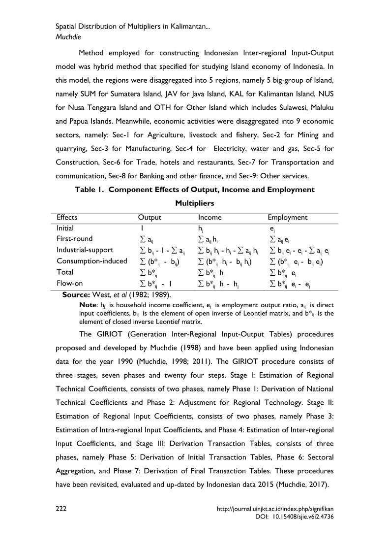
Method employed for constructing Indonesian Inter-regional Input-Output
model was hybrid method that specified for studying Island economy of Indonesia. In
this model, the regions were disaggregated into 5 regions, namely 5 big-group of Island,
namely SUM for Sumatera Island, JAV for Java Island, KAL for Kalimantan Island, NUS
for Nusa Tenggara Island and OTH for Other Island which includes Sulawesi, Maluku
and Papua Islands. Meanwhile, economic activities were disaggregated into 9 economic
sectors, namely: Sec-1 for Agriculture, livestock and fishery, Sec-2 for Mining and
quarrying, Sec-3 for Manufacturing, Sec-4 for Electricity, water and gas, Sec-5 for
Construction, Sec-6 for Trade, hotels and restaurants, Sec-7 for Transportation and
communication, Sec-8 for Banking and other finance, and Sec-9: Other services.
Table 1. Component Effects of Output, Income and Employment
Multipliers
Effects Output Income Employment
Initial 1 hj ej
First-round aij aij hi aij ei
Industrial-support bij - 1 - aij bij hi - hi - aij hi bij ei - ei - aij ei
Consumption-induced (b*ij - bij) (b*ij hi - bij hi) (b*ij ei - bij ei)
Total b*ij b*ij hi b*ij ei
Flow-on b*ij - 1 b*ij hi - hj b*ij ei - ej
Source: West, et al (1982; 1989).
Note: hj is household income coefficient, ej is employment output ratio, aij is direct
input coefficients, bij is the element of open inverse of Leontief matrix, and b*ij is the
element of closed inverse Leontief matrix.
The GIRIOT (Generation Inter-Regional Input-Output Tables) procedures
proposed and developed by Muchdie (1998) and have been applied using Indonesian
data for the year 1990 (Muchdie, 1998; 2011). The GIRIOT procedure consists of
three stages, seven phases and twenty four steps. Stage I: Estimation of Regional
Technical Coefficients, consists of two phases, namely Phase 1: Derivation of National
Technical Coefficients and Phase 2: Adjustment for Regional Technology. Stage II:
Estimation of Regional Input Coefficients, consists of two phases, namely Phase 3:
Estimation of Intra-regional Input Coefficients, and Phase 4: Estimation of Inter-regional
Input Coefficients, and Stage III: Derivation Transaction Tables, consists of three
phases, namely Phase 5: Derivation of Initial Transaction Tables, Phase 6: Sectoral
Aggregation, and Phase 7: Derivation of Final Transaction Tables. These procedures
have been revisited, evaluated and up-dated by Indonesian data 2015 (Muchdie, 2017).
http://journal.uinjkt.ac.id/index.php/signifikan 223 DOI: 10.15408/sjie.v6i2.4736
Signifikan Vol. 6 (2), Oktober 2017
One of the major uses of input-output information is to assess the effect on an
economy of changes in elements that are exogenous to the model of that economy.
The capabilities and usefulness of the Leontief inverse matrix, which is the source of
analytical power of the model are well known. However, the meaning and
interpretations are sometimes confusing.
As a measurement of response to an economic stimulus, a multiplier expresses
a cause and effect line of causality. In input-output analysis the stimulus is a change
(increase or decrease) in sales to final demand. Similar to those in the single-region
model, in the inter-regional model West et.al, in Muchdie (2011) defined the major
categories of response as: initial, first-round, industrial-support, consumption-induced,
total and flow-on effects. Formulas of such effects are provided in Table1.
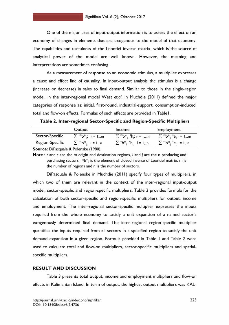
Table 2. Inter-regional Sector-Specific and Region-Specific Multipliers
Output Income Employment
Sector-Specific rsb*ij; r = 1,..m
rsb*ij shi; r = 1,..m
rsb*ij sei; r = 1,..m
Region-Specific rsb*ij; i = 1,..n
rsb*ij shi; i = 1,..n
rsb*ij sei; i = 1,..n
Source: DiPasquale & Polenske (1980).
Note : r and s are the m origin and destination regions, i and j are the n producing and
purchasing sectors, rsb*ij is the element of closed inverse of Leontief matrix, m is
the number of regions and n is the number of sectors.
DiPasquale & Polenske in Muchdie (2011) specify four types of multipliers, in
which two of them are relevant in the context of the inter-regional input-output
model; sector-specific and region-specific multipliers. Table 2 provides formula for the
calculation of both sector-specific and region-specific multipliers for output, income
and employment. The inter-regional sector-specific multiplier expresses the inputs
required from the whole economy to satisfy a unit expansion of a named sector’s
exogenously determined final demand. The inter-regional region-specific multiplier
quantifies the inputs required from all sectors in a specified region to satisfy the unit
demand expansion in a given region. Formula provided in Table 1 and Table 2 were
used to calculate total and flow-on multipliers, sector-specific multipliers and spatial-
specific multipliers.
RESULT AND DISCUSSION
Table 3 presents total output, income and employment multipliers and flow-on
effects in Kalimantan Island. In term of output, the highest output multipliers was KAL-
Spatial Distribution of Multipliers in Kalimantan...
Muchdie
224 http://journal.uinjkt.ac.id/index.php/signifikan
DOI: 10.15408/sjie.v6i2.4736
4 (Electricity, water and gas), 2.829. It means that an increase of final demand of the
sector by 1.000 would increase total output by 2.829 including the initial increase of
1.000. It was followed by KAL-9 (Other services), 2.808 meaning that an increase of
final demand of that sector by 1.000 would increase total output by 2.808 including the
initial increase of 1.000. The lowest total multipliers was in KAL-2 (Mining and
quarrying), 1.722. An increase of final demand of that sector by 1.000 units would
increase total output by 1.722 including the initial increase of 1.000. The flow-on
effects of output were the difference between total increase and initial increase. Flow-
on effect is summation of direct, indirect and induced effects of an economic activity. In
case of highest total multipliers (KAL-4) the flow-on effect was 1.829, meaning the
impact of increase of final demand of KAL-4 (Electricity, water and gas) to total output
was 1.829 as the initial effect was not included. The rank of total output multipliers
might be different than that of output flow-on effects. The evidence from Kalimantan
Island economy showed that the rank of total multipliers were the same as flow-on
effects where KAL-4 (Electricity, water and gas) had the highest output flow-on effects,
followed by KAL-9 (Other services) and the lowest value of output flow-on effects was
KAL-2 (Mining and quarrying).
In term of household income, the highest total income multiplier was in KAL-9
(Other services), 0.829. It means that an increase of final demand of KAL-9 (Other
services) by 1.000 units would increase initial household income by 0.593 and then
would increase total income by 0.829. It was followed by KAL-8 (Banking and other
finance) with total income multipliers of 0.489. The lowest total income multiplier was
in KAL-6 (Trade, hotel and restaurant) with total income multipliers of 0.338.
Income flow-on effects were the difference between total income multipliers
and initial income effects from the increase of final demand in that sector. It is the
summation of direct, indirect and induced effects of an economic activity. For instance,
in KAL-9 (Other services), the increase of final demand by 1.000 would have initial
income effects by 0.593, resulting total income of 0.829. The income flow-on effect of
KAL-9 (Other services) was 0.335. The highest income flow-on effect was in KAL-9
(Other services), followed by KAL-4 (Electricity, water and gas). The lowest income
flow-on effect was in, again, KAL-2 (Mining and quarrying).
http://journal.uinjkt.ac.id/index.php/signifikan 225 DOI: 10.15408/sjie.v6i2.4736
Signifikan Vol. 6 (2), Oktober 2017
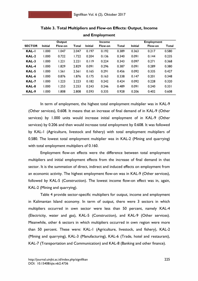
Table 3. Total Multipliers and Flow-on Effects: Output, Income
and Employment
SECTOR
Initial
Output
Flow-on
Total
Initial
Income
Flow-on
Total
Initial
Employment
Flow-on
Total
KAL-1 1.000 1.047 2.047 0.197 0.192 0.389 0.363 0.217 0.580
KAL-2 1.000 0.722 1.722 0.204 0.136 0.340 0.091 0.144 0.235
KAL-3 1.000 1.221 2.221 0.119 0.224 0.343 0.097 0.271 0.368
KAL-4 1.000 1.829 2.829 0.091 0.296 0.387 0.091 0.289 0.380
KAL-5 1.000 1.561 2.561 0.165 0.291 0.456 0.092 0.335 0.427
KAL-6 1.000 0.876 1.876 0.175 0.163 0.338 0.147 0.201 0.348
KAL-7 1.000 1.223 2.223 0.182 0.242 0.424 0.092 0.228 0.320
KAL-8 1.000 1.253 2.253 0.243 0.246 0.489 0.091 0.240 0.331
KAL-9 1.000 1.808 2.808 0.593 0.335 0.928 0.206 0.402 0.608
In term of employment, the highest total employment multiplier was in KAL-9
(Other services), 0.608. It means that an increase of final demand of in KAL-9 (Other
services) by 1.000 units would increase initial employment of in KAL-9 (Other
services) by 0.206 and then would increase total employment by 0.608. It was followed
by KAL-1 (Agriculture, livestock and fishery) with total employment multipliers of
0.580. The lowest total employment multiplier was in KAL-2 (Mining and quarrying)
with total employment multipliers of 0.160.
Employment flow-on effects were the difference between total employment
multipliers and initial employment effects from the increase of final demand in that
sector. It is the summation of direct, indirect and induced effects on employment from
an economic activity. The highest employment flow-on was in KAL-9 (Other services),
followed by KAL-5 (Construction). The lowest income flow-on effect was in, again,
KAL-2 (Mining and quarrying).
Table 4 provide sector-specific multipliers for output, income and employment
in Kalimantan Island economy. In term of output, there were 3 sectors in which
multipliers occurred in own sector were less than 50 percent, namely KAL-4
(Electricity, water and gas), KAL-5 (Construction), and KAL-9 (Other services).
Meanwhile, other 6 sectors in which multipliers occurred in own region were more
than 50 percent. These were: KAL-1 (Agriculture, livestock, and fishery), KAL-2
(Mining and quarrying), KAL-3 (Manufacturing), KAL-6 (Trade, hotel and restaurant),
KAL-7 (Transportation and Communication) and KAL-8 (Banking and other finance).
Spatial Distribution of Multipliers in Kalimantan...
Muchdie
226 http://journal.uinjkt.ac.id/index.php/signifikan
DOI: 10.15408/sjie.v6i2.4736
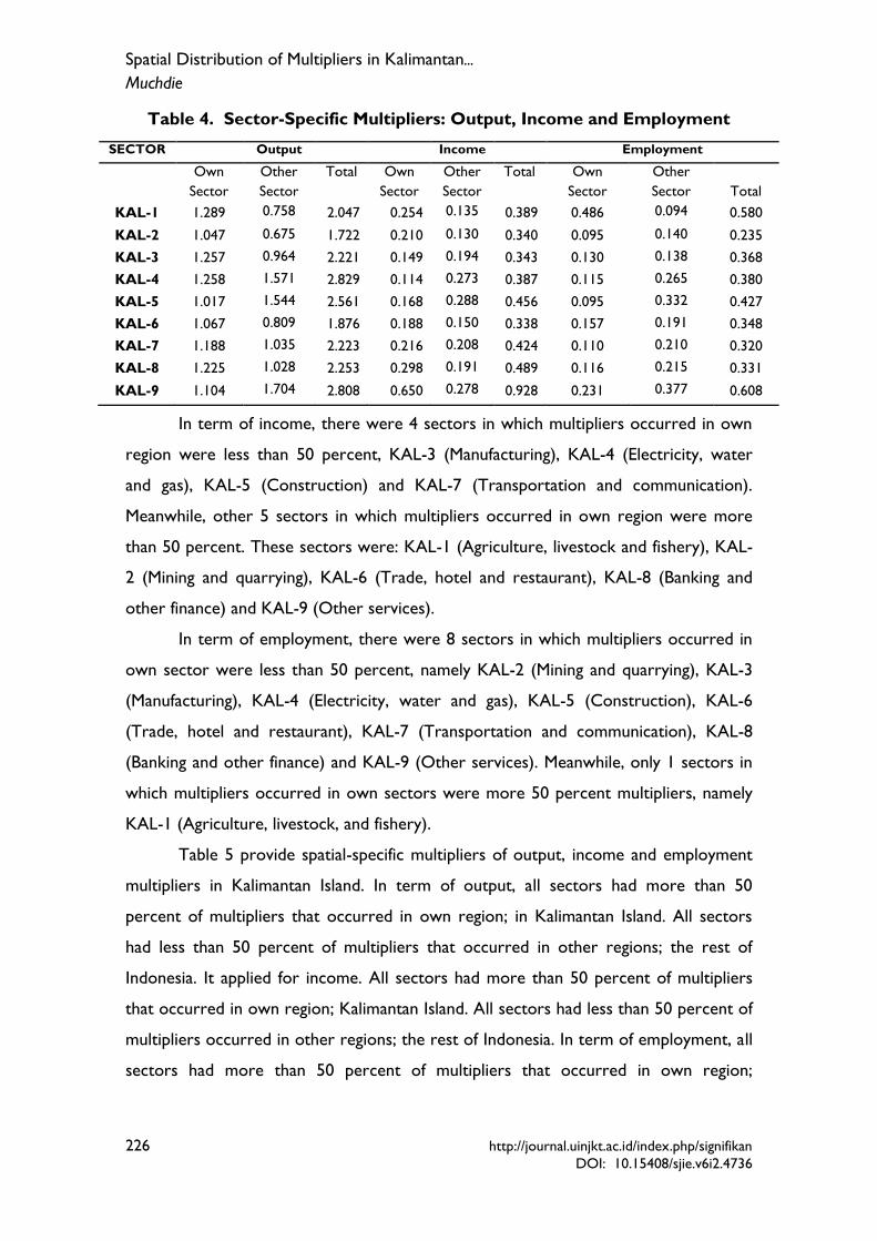
Table 4. Sector-Specific Multipliers: Output, Income and Employment
SECTOR Output Income Employment
Own
Sector
Other
Sector
Total Own
Sector
Other
Sector
Total Own
Sector
Other
Sector
Total
KAL-1 1.289 0.758 2.047 0.254 0.135 0.389 0.486 0.094 0.580
KAL-2 1.047 0.675 1.722 0.210 0.130 0.340 0.095 0.140 0.235
KAL-3 1.257 0.964 2.221 0.149 0.194 0.343 0.130 0.138 0.368
KAL-4 1.258 1.571 2.829 0.114 0.273 0.387 0.115 0.265 0.380
KAL-5 1.017 1.544 2.561 0.168 0.288 0.456 0.095 0.332 0.427
KAL-6 1.067 0.809 1.876 0.188 0.150 0.338 0.157 0.191 0.348
KAL-7 1.188 1.035 2.223 0.216 0.208 0.424 0.110 0.210 0.320
KAL-8 1.225 1.028 2.253 0.298 0.191 0.489 0.116 0.215 0.331
KAL-9 1.104 1.704 2.808 0.650 0.278 0.928 0.231 0.377 0.608
In term of income, there were 4 sectors in which multipliers occurred in own
region were less than 50 percent, KAL-3 (Manufacturing), KAL-4 (Electricity, water
and gas), KAL-5 (Construction) and KAL-7 (Transportation and communication).
Meanwhile, other 5 sectors in which multipliers occurred in own region were more
than 50 percent. These sectors were: KAL-1 (Agriculture, livestock and fishery), KAL-
2 (Mining and quarrying), KAL-6 (Trade, hotel and restaurant), KAL-8 (Banking and
other finance) and KAL-9 (Other services).
In term of employment, there were 8 sectors in which multipliers occurred in
own sector were less than 50 percent, namely KAL-2 (Mining and quarrying), KAL-3
(Manufacturing), KAL-4 (Electricity, water and gas), KAL-5 (Construction), KAL-6
(Trade, hotel and restaurant), KAL-7 (Transportation and communication), KAL-8
(Banking and other finance) and KAL-9 (Other services). Meanwhile, only 1 sectors in
which multipliers occurred in own sectors were more 50 percent multipliers, namely
KAL-1 (Agriculture, livestock, and fishery).
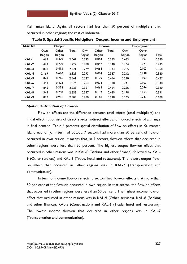
Table 5 provide spatial-specific multipliers of output, income and employment
multipliers in Kalimantan Island. In term of output, all sectors had more than 50
percent of multipliers that occurred in own region; in Kalimantan Island. All sectors
had less than 50 percent of multipliers that occurred in other regions; the rest of
Indonesia. It applied for income. All sectors had more than 50 percent of multipliers
that occurred in own region; Kalimantan Island. All sectors had less than 50 percent of
multipliers occurred in other regions; the rest of Indonesia. In term of employment, all
sectors had more than 50 percent of multipliers that occurred in own region;
http://journal.uinjkt.ac.id/index.php/signifikan 227 DOI: 10.15408/sjie.v6i2.4736
Signifikan Vol. 6 (2), Oktober 2017
Kalimantan Island. Again, all sectors had less than 50 percent of multipliers that
occurred in other regions; the rest of Indonesia.
Table 5. Spatial-Specific Multipliers: Output, Income and Employment
SECTOR Output Income Employment
Own
Region
Other
Region
Total Own
Region
Other
Region
Total Own
Region
Other
Region
Total
KAL-1 1.668 0.379 2.047 0.325 0.064 0.389 0.483 0.097 0.580
KAL-2 1.423 0.299 1.722 0.288 0.052 0.340 0.164 0.071 0.235
KAL-3 1.808 0.413 2.221 0.279 0.064 0.343 0.265 0.103 0.368
KAL-4 2.169 0.660 2.829 0.293 0.094 0.387 0.242 0.138 0.380
KAL-5 1.845 0.716 2.561 0.327 0.129 0.456 0.230 0.197 0.427
KAL-6 1.453 0.423 1.876 0.264 0.074 0.338 0.241 0.107 0.348
KAL-7 1.845 0.378 2.223 0.361 0.063 0.424 0.226 0.094 0.320
KAL-8 1.545 0.708 2.253 0.357 0.132 0.489 0.178 0.153 0.331
KAL-9 1.827 0.981 2.808 0.760 0.168 0.928 0.365 0.243 0.608
Spatial Distribution of Flow-on
Flow-on effects are the difference between total effects (total multipliers) and
initial effect. It consists of direct effects, indirect effect and induced effects of a change
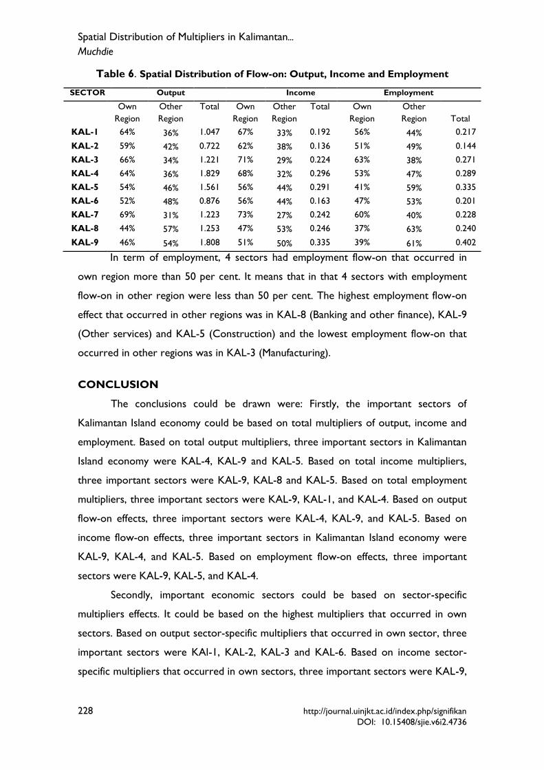
in final demand. Table 6 presents spatial distribution of flow-on effects in Kalimantan
Island economy. In term of output, 7 sectors had more than 50 percent of flow-on
occurred in own region. It means that, in 7 sectors, flow-on effects that occurred in
other regions were less than 50 percent. The highest output flow-on effect that
occurred in other regions was in KAL-8 (Banking and other finance), followed by KAL-
9 (Other services) and KAL-6 (Trade, hotel and restaurant). The lowest output flow-
on effect that occurred in other regions was in KAL-7 (Transportation and
communication).
In term of income flow-on effects, 8 sectors had flow-on effects that more than
50 per cent of the flow-on occurred in own region. In that sector, the flow-on effects
that occurred in other regions were less than 50 per cent. The highest income flow-on
effect that occurred in other regions was in KAL-9 (Other services), KAL-8 (Banking
and other finance), KAL-5 (Construction) and KAL-6 (Trade, hotel and restaurant).
The lowest income flow-on that occurred in other regions was in KAL-7
(Transportation and communication).
Spatial Distribution of Multipliers in Kalimantan...
Muchdie
228 http://journal.uinjkt.ac.id/index.php/signifikan
DOI: 10.15408/sjie.v6i2.4736
Table 6. Spatial Distribution of Flow-on: Output, Income and Employment
SECTOR Output Income Employment
Own
Region
Other
Region
Total Own
Region
Other
Region
Total Own
Region
Other
Region
Total
KAL-1 64% 36% 1.047 67% 33% 0.192 56% 44% 0.217
KAL-2 59% 42% 0.722 62% 38% 0.136 51% 49% 0.144
KAL-3 66% 34% 1.221 71% 29% 0.224 63% 38% 0.271
KAL-4 64% 36% 1.829 68% 32% 0.296 53% 47% 0.289
KAL-5 54% 46% 1.561 56% 44% 0.291 41% 59% 0.335
KAL-6 52% 48% 0.876 56% 44% 0.163 47% 53% 0.201
KAL-7 69% 31% 1.223 73% 27% 0.242 60% 40% 0.228
KAL-8 44% 57% 1.253 47% 53% 0.246 37% 63% 0.240
KAL-9 46% 54% 1.808 51% 50% 0.335 39% 61% 0.402
In term of employment, 4 sectors had employment flow-on that occurred in
own region more than 50 per cent. It means that in that 4 sectors with employment
flow-on in other region were less than 50 per cent. The highest employment flow-on
effect that occurred in other regions was in KAL-8 (Banking and other finance), KAL-9
(Other services) and KAL-5 (Construction) and the lowest employment flow-on that
occurred in other regions was in KAL-3 (Manufacturing).
CONCLUSION
The conclusions could be drawn were: Firstly, the important sectors of
Kalimantan Island economy could be based on total multipliers of output, income and
employment. Based on total output multipliers, three important sectors in Kalimantan
Island economy were KAL-4, KAL-9 and KAL-5. Based on total income multipliers,
three important sectors were KAL-9, KAL-8 and KAL-5. Based on total employment
multipliers, three important sectors were KAL-9, KAL-1, and KAL-4. Based on output
flow-on effects, three important sectors were KAL-4, KAL-9, and KAL-5. Based on
income flow-on effects, three important sectors in Kalimantan Island economy were
KAL-9, KAL-4, and KAL-5. Based on employment flow-on effects, three important
sectors were KAL-9, KAL-5, and KAL-4.
Secondly, important economic sectors could be based on sector-specific
multipliers effects. It could be based on the highest multipliers that occurred in own
sectors. Based on output sector-specific multipliers that occurred in own sector, three
important sectors were KAl-1, KAL-2, KAL-3 and KAL-6. Based on income sector-
specific multipliers that occurred in own sectors, three important sectors were KAL-9,
http://journal.uinjkt.ac.id/index.php/signifikan 229 DOI: 10.15408/sjie.v6i2.4736
Signifikan Vol. 6 (2), Oktober 2017
KAL-1, and KAL-2. Based on employment sector-specific multipliers that occurred in
own sector, three important sectors were KAL-1, KAL-6, and KAL-2.
Thirdly, important economic sectors could be based on spatial-specific
multipliers. It could be based on the highest multipliers that occurred in own regions;
in Kalimantan. Based on output spatial-specific multipliers that occurred in own region,
three important sectors were KAL-7, KAL-2, KAL-1, and KAL-3. Based on income
sector-specific multipliers that occurred in own region, three important sectors were
KAL-2, KAL-7 and KAL-1. Based on employment spatial-specific multipliers that
occurred in own region, three important sectors were KAL-1, KAL-3 and KAL-7.
Fourthly, important economic sectors could be based on spatial distribution of
flow-on. It could be based on the highest flow-on that occurred in own regions; in
Kalimantan Island. Based on output spatial distribution of low-on that occurred in own
region, three important sectors were KAL-7, KAL-3 and KAL-1. Based on income
spatial distribution of low-on that occurred in own region, three important sectors
were KAL-7, KAL-3 and KAL-1. Based on employment spatial distribution of flow-on
that occurred in own region, three important sectors were KAL-3, KAL-7 and KAL-1.
REFERENCES
Ahiakpor, J.C.W. (2000). Hawtrey on the Keynesian Multiplier: A Question of
Cognitive Dissonance? History of Political Economy. 32 (4): 889-908.
Beemiller, R.M. (1990). Improving Accuracy by Combining Primary Data with RIMS:
Comment on Bourque. International Regional Science Review, 13 (1-2): 99-101.
Coughlin, C. & T.B. Mandelbaum. (1991). A Consumer's Guide to Regional Economic
Multipliers. Federal Reserve Bank of St. Louis Review. January/February 1991.19-32.
Grady, P. & R.A. Muller. (1988). On the use and misuse of input-output based impact
analysis in evaluation. The Canadian Journal of Program Evaluation. 2 (3): 49-61.
Hall, R. E. (2009). By How Much Does GDP Rise if the Government Buys More
Output? NBER Working Paper 15496. National Bureau of Economic Research.
Harris, P. (1997). Limitations on the use of regional economic impact multipliers by
practitioners: An application to the tourism industry. The Journal of Tourism
Studies. 8(2): 1-12.
Spatial Distribution of Multipliers in Kalimantan...
Muchdie
230 http://journal.uinjkt.ac.id/index.php/signifikan
DOI: 10.15408/sjie.v6i2.4736
Hughes, D.W, (2003). Policy Uses of Economic Multipliers and Impact Analysis. Choices
Publication of the American Agricultural Economics Association, Second
Quarter.
Hulu, E (1990). Model Input-Output: Teori dan Applikasinya (Input-Output Model: Theory
and Its Applications). Jakarta: Pusat Antar Universitas- Universitas Indonesia.
Krugman, P & R. Wells. (2009). Economics. New York: Worth Publisher.
Mankiw, N. G (2008), Macroeconomics. New York: South-Western Publishing.
McConnell, C., S. Brue, & S. Flynn. (2011). Macroeconomics. New York: McGraw-Hill.
Mills, E. C. (1993). The Misuse of Regional Economic Models. Cato Journal, 13(1): 29-39.
Muchdie. (1998). Spatial Structure of Island Economy of Indonesia: An Inter-Regional
Input-Output Study. (Unpublished Dissertation). Quensland: the University of
Queensland, Australia.
Muchdie. (2011). Spatial Structure of Island Economy of Indonesia: A New Hybrid for
Generation Inter-regional Input-Output Tables. Germany: Lambert Academic
Publishing.
Muchdie. (2017). GIRIOT revisited, up-dated and evaluated, International Journal of
Social Science and Economic Research. 2(02): 2377-2396.
Pindyck, R & Rubinfeld, D (2012). Macroeconomics. London: The Pearson Series in
Economics.
Prihawantoro, S., I. Suryawijaya., R. Hutapea., U. Sugarmansyah., Alkadri., W.
Rusiawan., & M.Y. Permana. (2013). Peranan Teknologi Dalam Pertumbuhan
Koridor-Koridor Ekonomi Indonesia: Pendekatan Total Factor Productivity (The Role of
Technology in Economic Growth in Indonesian Economic Corridors: Total Factor
Productivity Approach). Jakarta: Badan Pengkajian dan Penerapan Teknologi.
Siegfried, J, R. Allen., A.R. Sanderson., & P. McHenry. (2006). The Economic Impact of
Colleges and Universities. Working Paper No. 06-W12.