Embed Size (px)
Citation preview

© Joseph J. Nahas 2012 10 Dec 2012
Statistical Design of Experiments Part I Overview
Joseph J. Nahas
1

2© Joseph J. Nahas 2012
10 Dec 2012
Quality in Japan• After WWII, Japan restarted their economy by manufacturing
inexpensive, low quality goods.• By the mid‐1970’s, Japanese car makers, Toyota, Honda, and
Nissan, began entering the US market with small, inexpensive cars, the Corolla, the Civic, and the Datsun.
• By the mid‐1980’s, people began to realize that these Japanese cars outlasted American cars by factors of 2 or
more.– American cars were worn‐out by 50k to 75k miles while many
Japanese cars lasted over 100,000 miles!
• Why?

3© Joseph J. Nahas 2012
10 Dec 2012
W. Edwards Deming• W. Edwards Deming was an American who learned statistical technology
from Walter Shewart of Bell Labs. He applied his learning first in the
Department of Agriculture and later in WWII. After the war, he was sent
to Japan to help the Japanese with their census. He stayed on, at the
request of Japanese Union of Scientists and Engineers to help Japanese
industry with statistical techniques. Because of his work in improving the
quality of Japanese industry, the Japanese quality award is named the
Deming Award.

4© Joseph J. Nahas 2012
10 Dec 2012
Genichi Taguchi• Genichi Taguchi was initially trained as a textile engineer. After WWII he
joined the Electrical Communications Laboratory (ECL) of the Nippon
Telegraph and Telephone Corporation where he came under the influence
of W. Edwards Deming. In 1954‐1955 was visiting professor at the Indian
Statistical Institute where he was introduced to the orthogonal arrays
which became the foundation of his later work. He finished his doctorate
in 1962 and became a professor of engineering at Aoyama Gakuin
University, Tokyo where consulted with industry propagating what
became known as Taguchi Methods.
5© Joseph J. Nahas 2012
10 Dec 2012
Taguchi Methods• Off‐line Quality Control
– Use experimental design techniques
to both improve a process and to
reduce output variation.Need to reduce a processes sensitivity to uncontrolled parametervariation.
– The use a controllable parameter to re‐center the design where is best
fits the product.
• Example: Internal combustion engine cylinder and piston.
6© Joseph J. Nahas 2012
10 Dec 2012
Orthogonal Array Methods• Not new fromTaguchi• Wide statistics literature on the subject.• Taguchi make it accessible to engineers and propagated a
limited set of methods that simplified the use of orthogonal arrays.
• Design of Experiments (DoE) is primarily covered in Section 5, Process Improvement of the NIST ESH.
NIST ESH 5
7© Joseph J. Nahas 2012
10 Dec 2012
Outline1.
Introduction
2.
Design of Experiments Basics3.
Full Factorial Designs Simple ExampleA.
2n
DesignsB.
Single FactorC.
2 Factor Plots
4.
Fractional Factorial Designs Arrays
8© Joseph J. Nahas 2012
10 Dec 2012
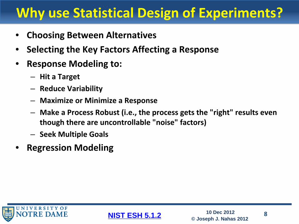
Why use Statistical Design of Experiments?• Choosing Between Alternatives• Selecting the Key Factors Affecting a Response• Response Modeling to:
– Hit a Target– Reduce Variability– Maximize or Minimize a Response– Make a Process Robust (i.e., the process gets the "right" results even
though there are uncontrollable "noise" factors)– Seek Multiple Goals
• Regression Modeling
NIST ESH 5.1.2
9© Joseph J. Nahas 2012
10 Dec 2012
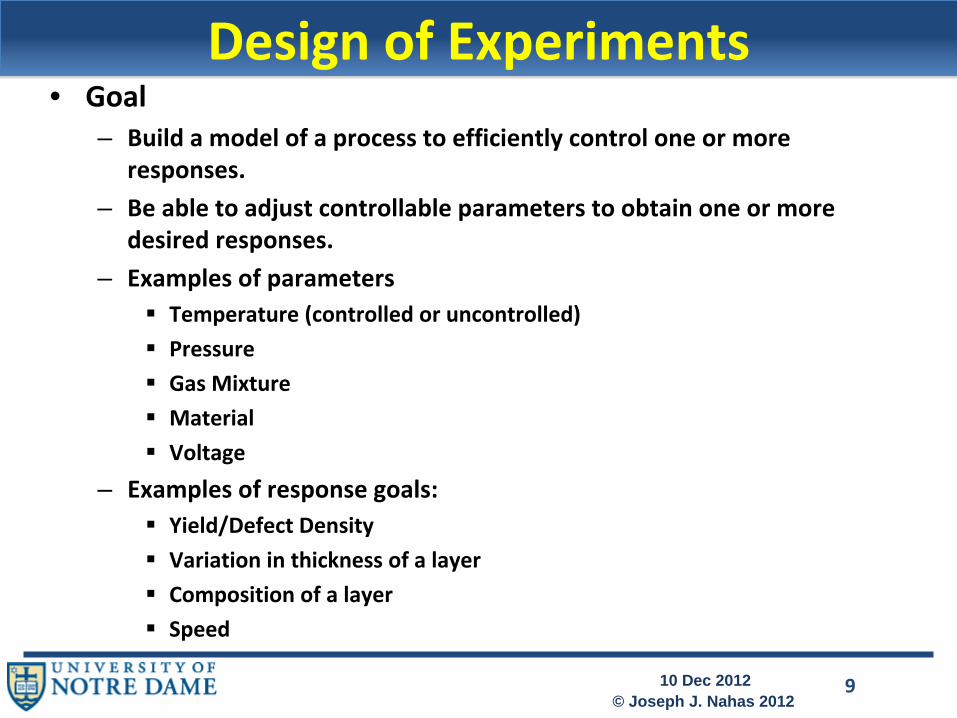
Design of Experiments• Goal
– Build a model of a process to efficiently control one or more
responses.– Be able to adjust controllable parameters to obtain one or more
desired responses.– Examples of parameters
Temperature (controlled or uncontrolled)PressureGas MixtureMaterialVoltage
– Examples of response goals:Yield/Defect DensityVariation in thickness of a layerComposition of a layerSpeed
10© Joseph J. Nahas 2012
10 Dec 2012
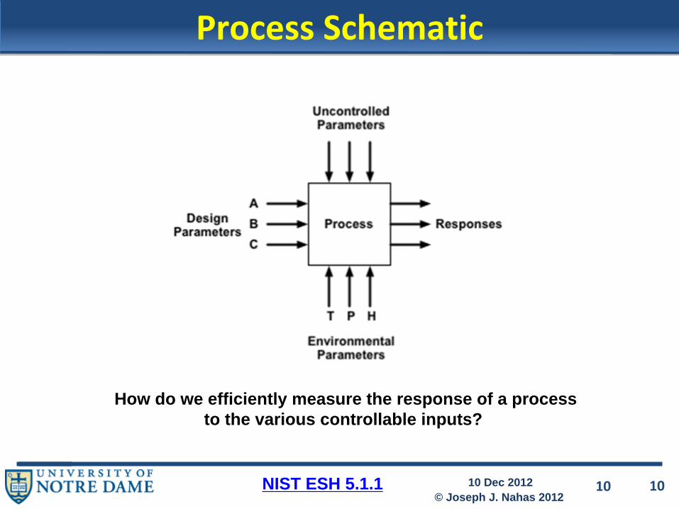
Process Schematic
10
How do we efficiently measure the response of a processto the various controllable inputs?
NIST ESH 5.1.1
11© Joseph J. Nahas 2012
10 Dec 2012
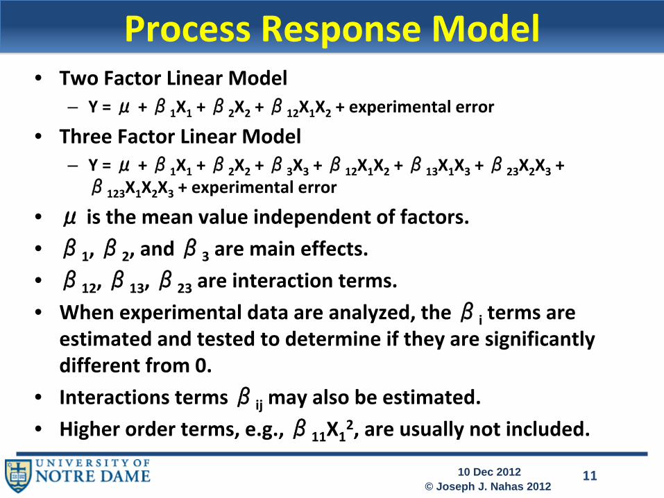
Process Response Model• Two Factor Linear Model
– Y = μ + β1
X1
+ β2
X2
+ β12
X1
X2
+ experimental error
• Three Factor Linear Model– Y = μ + β1
X1
+ β2
X2
+ β3
X3
+ β12
X1
X2
+ β13
X1
X3
+ β23
X2
X3
+
β123
X1
X2
X3
+ experimental error
• μ is the mean value independent of factors.• β1
, β2
, and β3
are main effects.• β12
, β13
, β23
are interaction terms.• When experimental data are analyzed, the βi
terms are estimated and tested to determine if they are significantly
different from 0. • Interactions terms βij
may also be estimated.• Higher order terms, e.g., β11
X12, are usually not included.
12© Joseph J. Nahas 2012
10 Dec 2012
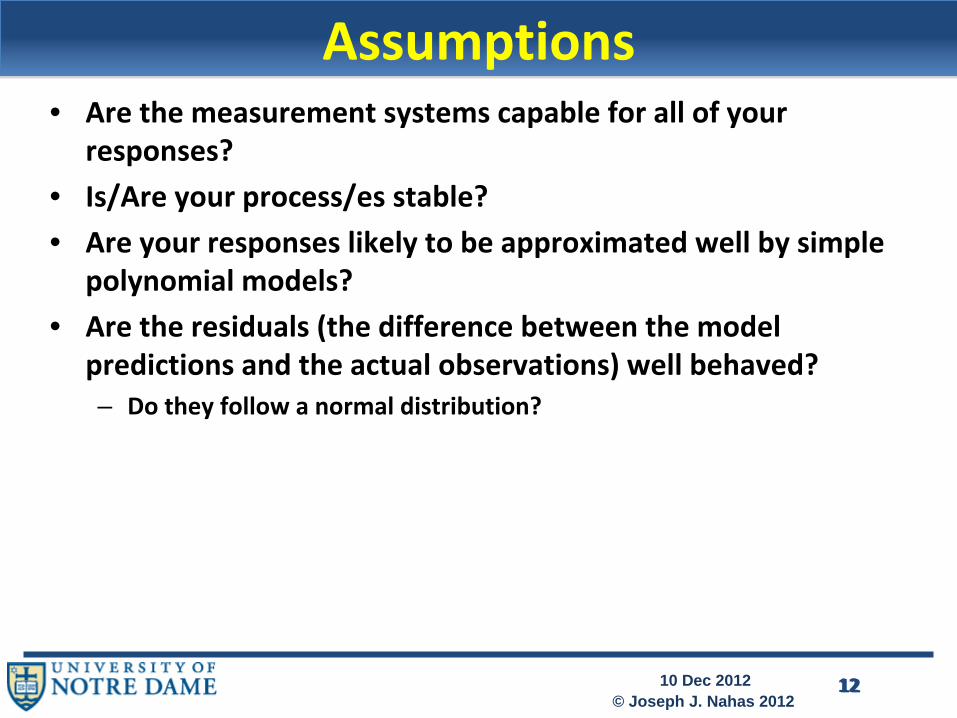
Assumptions• Are the measurement systems capable for all of your
responses?• Is/Are your process/es stable?• Are your responses likely to be approximated well by simple
polynomial models?• Are the residuals (the difference between the model
predictions and the actual observations) well behaved?– Do they follow a normal distribution?
12
13© Joseph J. Nahas 2012
10 Dec 2012
Outline1.
Introduction
2.
Design of Experiments Basics3.
Full Factorial Designs Simple ExampleA.
2n
DesignsB.
Single FactorC.
2 Factor Plots
4.
Fractional Factorial Designs Arrays
14© Joseph J. Nahas 2012
10 Dec 2012
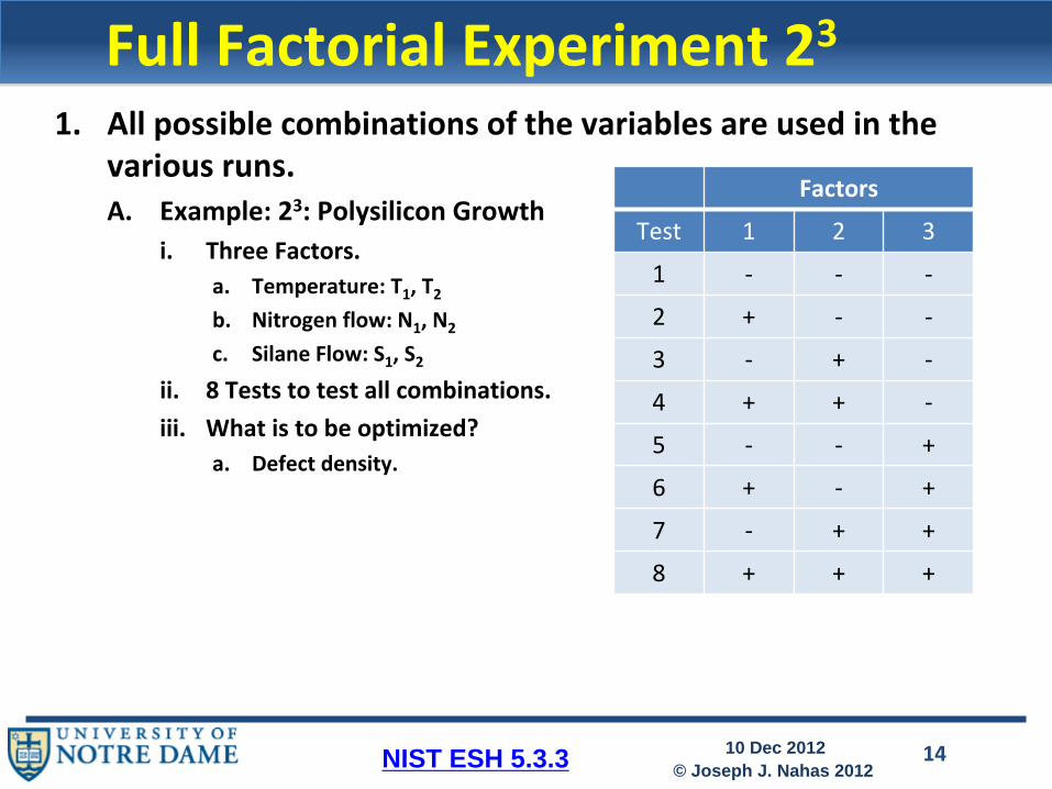
Full Factorial Experiment 231.
All possible combinations of the variables are used in the
various runs.A.
Example: 23: Polysilicon Growthi.
Three Factors.a.
Temperature: T1
, T2b.
Nitrogen flow: N1
, N2
c.
Silane Flow: S1
, S2ii.
8 Tests to test all combinations.iii.
What is to be optimized?a.
Defect density.
Factors
Test 1 2 3
1 ‐ ‐ ‐
2 + ‐ ‐
3 ‐ + ‐
4 + + ‐
5 ‐ ‐ +
6 + ‐ +
7 ‐ + +
8 + + +
NIST ESH 5.3.3
15© Joseph J. Nahas 2012
10 Dec 2012
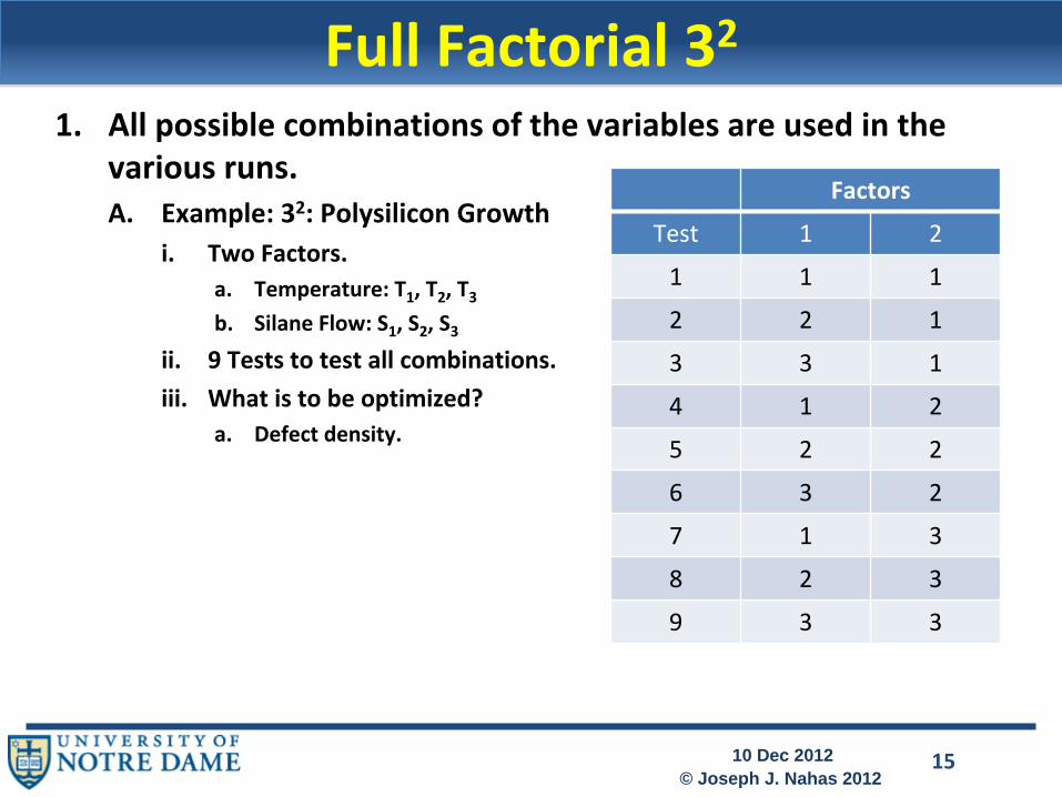
Full Factorial 321.
All possible combinations of the variables are used in the
various runs.A.
Example: 32: Polysilicon Growthi.
Two Factors.a.
Temperature: T1
, T2
, T3b.
Silane Flow: S1
, S2
, S3ii.
9 Tests to test all combinations.iii.
What is to be optimized?a.
Defect density.
Factors
Test 1 2
1 1 1
2 2 1
3 3 1
4 1 2
5 2 2
6 3 2
7 1 3
8 2 3
9 3 3
16© Joseph J. Nahas 2012
10 Dec 2012
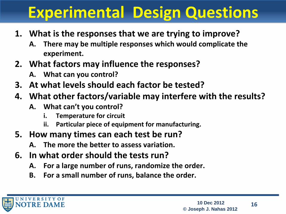
Experimental Design Questions1.
What is the responses that we are trying to improve?A.
There may be multiple responses which would complicate the
experiment.2.
What factors may influence the responses?A.
What can you control?3.
At what levels should each factor be tested?
4.
What other factors/variable may interfere with the results?A.
What can’t you control?i.
Temperature for circuitii.
Particular piece of equipment for manufacturing.5.
How many times can each test be run?A.
The more the better to assess variation.6.
In what order should the tests run?A.
For a large number of runs, randomize the order.B.
For a small number of runs, balance the order.
17© Joseph J. Nahas 2012
10 Dec 2012
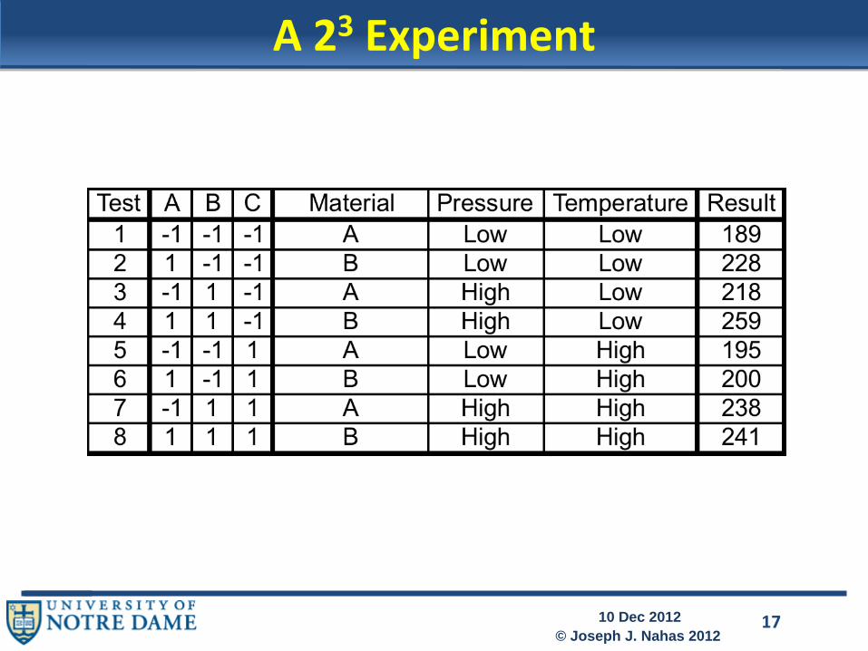
A 23
Experiment
18© Joseph J. Nahas 2012
10 Dec 2012
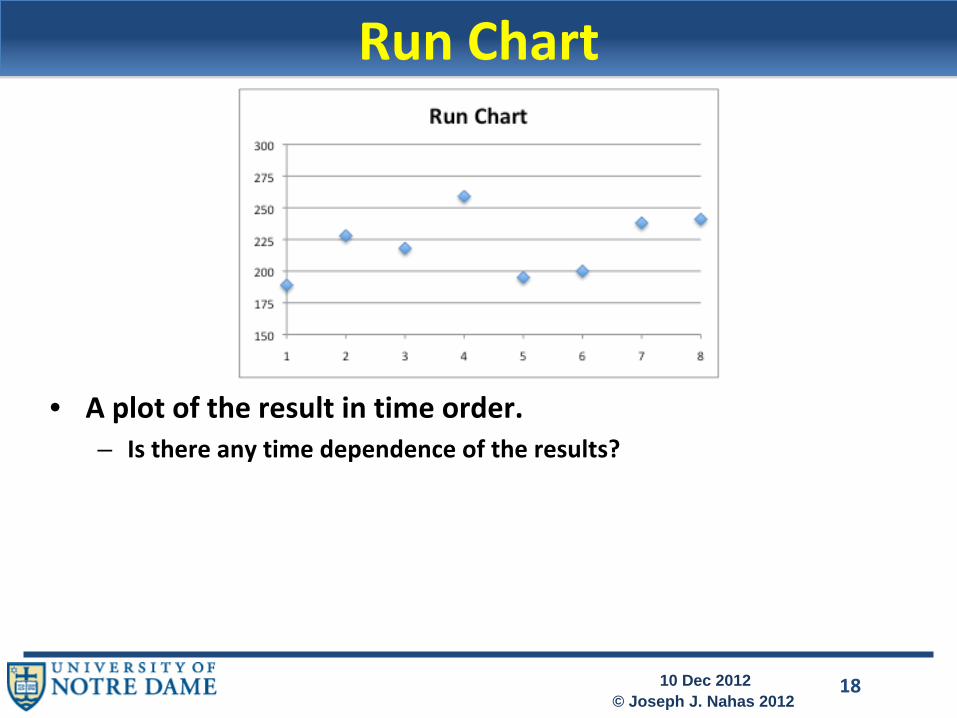
Run Chart
• A plot of the result in time order.– Is there any time dependence of the results?

19© Joseph J. Nahas 2012
10 Dec 2012
Response by Parameter
Each point averages theresponse for all the valuesof the other two variables.

20© Joseph J. Nahas 2012
10 Dec 2012
Pressure and Temperature Response vs Material
No Dependence
Large Dependence
Each point averages theresponse of the two valuesof the other variable.
21© Joseph J. Nahas 2012
10 Dec 2012
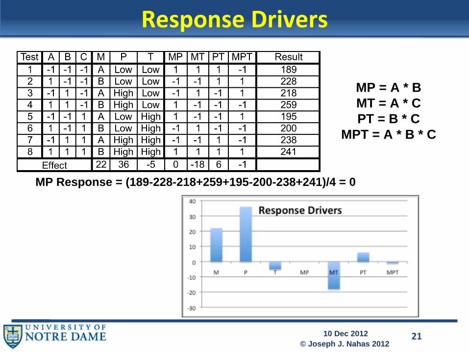
Response Drivers
MP Response = (189-228-218+259+195-200-238+241)/4 = 0
MP = A * BMT = A * CPT = B * C
MPT = A * B * C
22© Joseph J. Nahas 2012
10 Dec 2012
Outline1.
Introduction
2.
Design of Experiments Basics3.
Full Factorial Designs Simple ExampleA.
2n
DesignsB.
Single FactorC.
2 Factor Plots
4.
Fractional Factorial Designs Arrays

23© Joseph J. Nahas 2012
10 Dec 2012
Fractional Factorial 23‐1• Not all parameter combinations are tested.• Parameter values are balanced against every other
parameter.• Example: 23‐1
Note balance for each parameter:o Each value of A has both values for B and C.o Each value of B has both values for A and C.o Each value of C has both values for A and B.
Parameter
Test A B C
1 1 1 1
2 1 2 2
3 2 1 2
4 2 2 1
NIST ESH 5.3.3.4

24© Joseph J. Nahas 2012
10 Dec 2012
Fractional Factorial 27‐4• Not all parameter combinations are tested.• Parameter values are balanced against every other
parameter.– i. e. the array is orthogonal.
• Example: 27‐4Note balance for each parameter:
o Each value of A has both values for B, C, D, E, F, and G.o Each value of B has both values for A, C, D, E, F, and G.o Each value of C has both values for A, B, D, E, G and G.o Etc.
Parameter
A B C D E F G
1 1 1 1 1 1 1 1
2 1 1 1 2 2 2 2
3 1 2 2 1 1 2 2
4 1 2 2 2 2 1 1
5 2 1 2 1 2 1 2
6 2 1 2 2 1 2 1
7 2 2 1 1 2 2 1
8 2 2 1 2 1 1 2