Statistics and Econometrics I - 國立臺灣大學homepage.ntu.edu.tw/~sschen/Teaching/Lecture8_Asymptotics_2016.… · Statistics and Econometrics I Asymptotic Theory Shiu-Sheng

Statistics and Econometrics I

Asymptotic Theory

Shiu-Sheng Chen

Department of Economics

National Taiwan University

September 13, 2016

Shiu-Sheng Chen (NTU Econ) Statistics and Econometrics I September 13, 2016 1 / 30

Asymptotic Theory: Motivation

Asymptotic theory or large sample theory aims at answering the

question: what happens as we gather more and more data?

In particular, given random sample, {X1, X2, X3, . . . , Xn}, and

statistic:

Tn = t(X1, X2, . . . , Xn),

what is the limiting behavior of Tn as n −→∞?


Asymptotic Theory: Motivation

Why asking such a question?

For instance, given random sample {Xi}ni=1 ∼i.i.d. N(µ, σ2), we know

that

X̄n ∼ N(µ,σ2

n

)However, if {Xi}ni=1 ∼i.i.d. (µ, σ2), what is the distribution of X̄n?

I We don’t know, indeed.

Is it possible to find a good approximation of the distribution of X̄n

as n −→∞?


Part I

Preliminary Knowledge




Limit

Markov Inequality

Chebyshev Inequality



Limit of a Real Sequence

Definition (Limit)

If for every ε > 0, and an integer N(ε),

|bn − b| < ε, ∀ n > N(ε)

then we say that a sequence of real numbers {b1, . . . , bn} converges to a

limit b.

It is denoted by

limn→∞

bn = b



Markov Inequality

Theorem (Markov Inequality)

Suppose that X is a random variable such that P (X ≥ 0) = 1. Then for

every real number m > 0,

P (X ≥ m) ≤ E(X)

m



Chebyshev Inequality

Theorem (Chebyshev Inequality)

Let Y ∼ (E(Y ), V ar(Y )). Then for every number ε > 0,

P(∣∣Y − E(Y )

∣∣ ≥ ε) ≤ V ar(Y )

ε2

Proof: Let X = [Y − E(Y )]2, then

P (X ≥ 0) = 1

and

E(X) = V ar(Y )

Hence, the result can be derived by applying the Markov Inequality.


Part II

Modes of Convergence



Types of Convergence

For a random variable, we consider three modes of convergence:

Converge in Probability

Converge in Distribution

Converge in Mean Square




Definition (Converge in Probability)

Let {Yn} be a sequence of random variables and let Y be another random

variable. For any ε > 0,

P (|Yn − Y | < ε) −→ 1, as n −→∞

then we say that Yn converges in probability to Y , and denote it by

Ynp−→ Y

Equivalently,

P (|Yn − Y | ≥ ε) −→ 0, as n −→∞




{Xi}ni=1 ∼i.i.d. Bernoulli(0.5) and then compute Yn = X̄n =∑

iXi

n

In this case, Ynp−→ 0.5

Total Flips

X

0 200 400 600 800 1000

0.2

0.4

0.6

0.8

1.0



Converge in Distribution

Definition (Converge in Distribution)

Let {Yn} be a sequence of random variables with distribution function

FYn(y), (denoted by Fn(y) for simplicity). Let Y be another random

variable with distribution function, FY (y). If

limn→∞

Fn(y) = FY (y) at all y for which FY (y) is continuous

then we say that Yn converges in distribution to Y .

It is denoted by

Ynd−→ Y

FY (y) is called the limiting distribution of Yn.



Converge in Mean Square

Definition (Converge in Mean Square)

Let {Yn} be a sequence of random variables and let Y be another random

variable. If

E(Yn − Y )2 −→ 0, as n −→∞.

Then we say that Yn converges in mean square to Y .

It is denoted by

Ynms−→ Y

It is also called converge in quadratic mean.


Part III

Important Theorems


Important Theorems

Theorems

Theorem

Ynms−→ c if and only if

limn→∞

E(Yn) = c, and limn→∞

V ar(Yn) = 0.

Proof. It can be shown that

E(Yn − c)2 = E([Yn − E(Yn)]2) + [E(Yn)− c]2


Important Theorems

Theorems

Theorem

If Ynms−→ Y then Yn

p−→ Y

Proof: Note that P (|Yn − Y |2 ≥ 0) = 1, and by Markov Inequality,

P (|Yn − Y | ≥ k) = P (|Yn − Y |2 ≥ k2) ≤ E(|Yn − Y |2)

k2


Important Theorems

Weak Law of Large Numbers, WLLN

Theorem (WLLN)

Given a random sample {Xi}ni=1 with σ2 = V ar(X1) <∞. Let X̄n

denote the sample mean, and note that E(X̄n) = E(X1) = µ. Then

X̄np−→ µ

Proof: (1) By Chebyshev Inequality (2) By Converge in Mean Square

Sample mean X̄n is getting closer (in probability sense) to the

population mean µ as the sample size increases.

That is, if we use X̄n as a guess of unknown µ, we are quite happy

that the sample mean makes a good guess.


Important Theorems

WLLN for Other Moments

Note that the WLLN can be thought as∑ni=1Xi

n=X1 +X2 + · · ·Xn

n

p−→ E(X1)

Hence, ∑ni=1X

2i

n=X2

1 +X22 + · · ·X2

n

n

p−→ E(X21 )


Important Theorems

An Application of WLLN

Example: Assume Wn ∼ Binomial(n, µ), and let Yn = Wnn . Then

Ynp−→ µ

I Why?

I Since Wn =∑iXi, Xi ∼i.i.d.Bernoulli(µ) with E(X1) = µ,

V ar(X1) = µ(1− µ), the result follows by WLLN.


Important Theorems

An Application of WLLN

Example: Assume Wn ∼ Binomial(n, µ), and let Yn = Wnn . Then

Ynp−→ µ

I Why?

I Since Wn =∑iXi, Xi ∼i.i.d.Bernoulli(µ) with E(X1) = µ,

V ar(X1) = µ(1− µ), the result follows by WLLN.


Important Theorems

Central Limit Theorem, CLT

Theorem (CLT)

Let {Xi}ni=1 be a random sample, where E(X1) = µ <∞,

V ar(X1) = σ2 <∞, then

Zn =X̄n − E(X̄n)√V ar(X̄n)

=

√n(X̄n − µ)

σ

d−→ N(0, 1)

If a random sample is taken from any distribution with mean µ and

variance σ2, regardless of whether this distribution is discrete or

continuous, then the distribution of the random variable Zn will be

approximately the standard normal distribution in large sample.


Important Theorems

CLT

Using notation of asymptotic distribution,

X̄n − µ√σ2

n

∼A N(0, 1),

Or

X̄n ∼A N(µ,σ2

n

),

where ∼A represents asymptotic distribution, and A represents

Asymptotically


Important Theorems

An Application of CLT

Example: Assume {Xi} ∼i.i.d.Bernoulli(µ), then

X̄n − µ√µ(1−µ)

n

d−→ N(0, 1).

I Why?

I Since E(X̄n) = µ, and V ar(X̄n) = σ2

n = µ(1−µ)n


Important Theorems

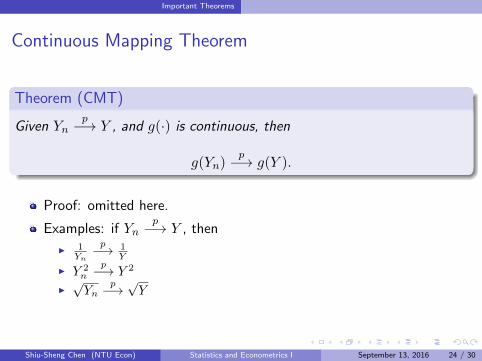
Continuous Mapping Theorem

Theorem (CMT)

Given Ynp−→ Y , and g(·) is continuous, then

g(Yn)p−→ g(Y ).

Proof: omitted here.

Examples: if Ynp−→ Y , then

I 1Yn

p−→ 1Y

I Y 2n

p−→ Y 2

I√Yn

p−→√Y


Important Theorems

Theorem

Theorem

Given Wnp−→W and Yn

p−→ Y , then

Wn + Ynp−→W + Y

WnYnp−→WY



Important Theorems

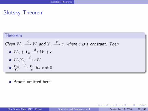
Slutsky Theorem

Theorem

Given Wnd−→W and Yn

p−→ c, where c is a constant. Then

Wn + Ynd−→W + c

WnYnd−→ cW

WnYn

d−→ Wc for c 6= 0



Important Theorems

The Delta Method

Theorem

Given√n(Yn − θ)

d−→ N(0, σ2). Let g(·) be differentiable, and g′(θ) 6= 0

exists, then√n(g(Yn)− g(θ))

d−→ N(0, [g′(θ)]2σ2).

Proof: (sketch) Given 1st-order Taylor approximation

g(Yn) ≈ g(θ) + g′(θ)(Yn − θ),

then √n(g(Yn)− g(θ))

g′(θ)≈√n(Yn − θ)

d−→ N(0, σ2)


Important Theorems

Example

Given {Xi}ni=1 ∼i.i.d. (µ, σ2), find the asymptotic distribution ofX̄n

1−X̄n.

I Note that by CLT,

√n(X̄n − µ)

d−→ N(0, σ2)

I Hence, by the Delta method,

g(X̄n) =X̄n

1− X̄n, g(µ) =

µ

1− µ, g′(µ) =

1

(1− µ)2

√n

(X̄n

1− X̄n− µ

1− µ

)d−→ N

(0,

1

(1− µ)4σ2

)


Important Theorems

Applications: Limiting Property of χ2 Random Variable

Theorem

Given Wn ∼ χ2(n), and let Xn = Wnn . Then

Xnp−→ 1


Important Theorems

Applications: Limiting Property of t Random Variable

Theorem

Given Un ∼ t(n), then

Und−→ N(0, 1)


Documents

Statistics and Econometrics I - 國立臺灣大學homepage.ntu.edu.tw/~sschen/Teaching/Lecture8_Asymptotics_2016.… · Statistics and Econometrics I Asymptotic Theory Shiu-Sheng