Embed Size (px)
Citation preview
Deutsche Geodätische Kommission
bei der Bayerischen Akademie der Wissenschaften
Reihe C Dissertationen Heft Nr. 660
Stefan Josef Auer
3D Synthetic Aperture Radar Simulation
for Interpreting Complex Urban Reflection Scenarios
München 2011
Verlag der Bayerischen Akademie der Wissenschaftenin Kommission beim Verlag C. H. Beck
ISSN 0065-5325 ISBN 978-3-7696-5072-3

Deutsche Geodätische Kommission
bei der Bayerischen Akademie der Wissenschaften
Reihe C Dissertationen Heft Nr. 660
3D Synthetic Aperture Radar Simulation
for Interpreting Complex Urban Reflection Scenarios
Vollständiger Abdruck
der von der Fakultät für Bauingenieur- und Vermessungswesen
der Technischen Universität München
zur Erlangung des akademischen Grades eines
Doktor-Ingenieurs (Dr.-Ing.)
genehmigten Dissertation
von
Dipl.-Ing. Stefan Josef Auer
München 2011
Verlag der Bayerischen Akademie der Wissenschaftenin Kommission beim Verlag C. H. Beck
ISSN 0065-5325 ISBN 978-3-7696-5072-3

Adresse der Deutschen Geodätischen Kommission:
Deutsche Geodätische KommissionAlfons-Goppel-Straße 11 ! D – 80 539 München
Telefon +49 – 89 – 23 031 1113 ! Telefax +49 – 89 – 23 031 - 1283 / - 1100e-mail [email protected] ! http://www.dgk.badw.de
Prüfungskommission
Vorsitzender: Univ.-Prof. Dr.-Ing. Dr. h.c. mult. Reiner Rummel
Prüfer der Dissertation: 1. Univ.-Prof. Dr.-Ing. habil. Richard Bamler
2. Univ.-Prof. Dr.-Ing. habil. Stefan Hinz, Universität Karlsruhe3. Prof. Antonio Iodice, Ph.D, Università degli Studi di Napoli Federico II, Italien
Die Dissertation wurde am 09.12.2010 bei der Technischen Universität München eingereichtund durch die Fakultät für Bauingenieur- und Vermessungswesen am 11.03.2011 angenommen.
© 2011 Deutsche Geodätische Kommission, München
Alle Rechte vorbehalten. Ohne Genehmigung der Herausgeber ist es auch nicht gestattet,die Veröffentlichung oder Teile daraus auf photomechanischem Wege (Photokopie, Mikrokopie) zu vervielfältigen.
ISSN 0065-5325 ISBN 978-3-7696-5072-3
3
Abstract
Due to the high spatial resolution of up to 1 m, very high resolution spaceborne SAR sensorssuch as TerraSAR-X/TanDEM-X or COSMO-SkyMed enable the monitoring of single objectson the earth surface. However, the interpretation of the appearance of objects on SAR imagesis difficult due to distortion effects like foreshortening or layover. So far, the nature of scatterersevoking prominent SAR image features is still not known in detail. Simulation methods based onrendering algorithms enable to support the visual interpretation of SAR images, as the focus canbe set on the object geometry. Mainly developed for providing test data sets, simulators reportedin the literature are limited to the azimuth-range plane. Additional methods for exploiting thegeometry of simulated data still have to be developed. In order to overcome these limitations,the work presented in this thesis adresses three new aspects. First, SAR simulation is conductedin three dimensions, including the elevation domain. Second, methods for the directed analysisof image signatures are introduced. Finally, the inversion of SAR imaging systems is simulatedfor analyzing the physical origin of SAR image signatures.
In order to meet these objectives, a SAR simulator named RaySAR has been developed basedon ray tracing methods which provides simulation products in three steps: modeling, sampling,and 3D analysis of scatterers. In the modeling step, the geometry and surface parameters ofobjects are defined within a virtual scene. Geometrical and radiometrical information aboutsignal contributions is captured by sampling the scene. To this end, POV-Ray, an open-sourceray tracer, is adapted in order to provide output data in SAR geometry. In this regard, anideal SAR system is simulated which is characterized by infinite resolution in azimuth, range,and elevation. Specular reflections are detected based on a geometrical analysis of the signalpath. In the last step, scatterers are analyzed in three dimensions based on images simulatedin the azimuth-range plane. Layover situations can be resolved due to the availability of 3Dinformation. Moreover, SAR image signatures can be linked with the geometry of simulatedobjects.
The results of different case studies show potentials and limitations of the simulation concept.With regard to the sampling step, limitations occur due to simplified reflection models and apartial loss of diffuse multiple reflections. However, RaySAR fully covers specular reflections andenables to simulate object models characterized by a high level of detail. Concerning the requiredlevel of detail of building models, at least basic facade details have to be geometrically described.Triple reflections at building corners are confirmed as prominent building hints on SAR images.In addition, signal reflections of bounce levels larger than 3 are likely to appear for isolatedbuildings. When using detailed building models, simulated signatures can be automaticallylinked to real SAR data. Thereafter, the inversion of the SAR imaging process is enabled byidentifying the corresponding scatterers on the 3D model of the simulated scene. The casestudies reveal, that a high number of SAR image signatures do not directly represent thegeometry of objects. For instance, multiple reflections may be localized in 3D space next tobuildings, on ground or even beneath the ground level.
4
Zusammenfassung
Aktuelle satellitengetragene SAR-Systeme wie TerraSAR-X/TanDEM-X oder COSMO-SkyMed ermoglichen die Uberwachung von Einzelobjekten an der Erdoberflache aufgrundihrer hohen raumliche Auflosung. Die Interpretation des Erscheinungsbilds von Objekten inSAR-Bildern ist dennoch schwierig aufgrund von Verzerrungseffekten wie der Verkurzung oderUberlagerung von Objektinformation. Die Natur von Streuern, die deutlich sichtbare SAR-Bildsignaturen hervorrufen, ist bislang noch nicht im Detail bekannt. Auf Render-Algorithmenbasierende Simulationsmethoden ermoglichen die Unterstutzung der visuellen Interpretationvon SAR-Bildern, indem das Augenmerk auf die Geometrie von Objekten gelegt werden kann.Bisher veroffentlichte Simulationsverfahren wurden hauptsachlich fur die Erzeugung von Test-datensatzen entwickelt und sind auf die Azimut-Entfernung-Ebene begrenzt. WeitergehendeMethoden fur die Auswertung der geometrischen Information simulierter Daten mussen nochentwickelt werden. Der in dieser Doktorarbeit prasentierte Ansatz spricht drei neue Aspektean, um diese Limitierungen zu uberwinden. Zum einen wird die Simulation von SAR-Daten indrei Dimensionen durchgefuhrt, einschließlich der Elevationsrichtung. Zudem werden Methodenaufgezeigt fur eine gesteuerte Analyse von Bildsignaturen. Schließlich wird die Inversion einesSAR-Abbildungssystems simuliert, um den physikalischen Ursprung von SAR-Bildsignaturenfeststellen zu konnen.
Fur die Realisierung dieser Ziele wurde ein SAR-Simulator namens RaySAR entwickelt, derauf Raytracing-Methoden basiert und Simulationsprodukte anhand von drei Arbeitsschrittenbereitstellt: Modellierung, Abtastung und 3D Analyse von Streuern. Der Modellierungsschrittbeinhaltet die Definition der Geometrie und Oberflache von Objekten innerhalb einer virtuellenSzene. Geometrische und radiometrische Informationen uber Signalbeitrage werden durch dieAbtastung der Szene erfasst. In diesem Zusammenhang wird ein ideales SAR-System simuliert,welches eine unendliche Auflosung in Azimut-, Entfernungs- und Elevationsrichtung besitzt.Spiegelnde Reflexionen werden erkannt anhand einer geometrischen Analyse des Signalpfads.Im letzten Arbeitsschritt werden auf der Grundlage von simulierten Bilddaten in der Azimut-Entfernung-Ebene Streuer im dreidimensionalen Raum analysiert. Uberlagerungseffekte inSAR-Bildern lassen sich dabei durch die Verfugbarkeit von 3D Information auflosen. Daruberhinaus konnen SAR-Bildsignaturen mit der Geometrie von simulierten Objekten in Verbindunggebracht werden.
Die Ergebnisse von verschiedenen Fallstudien zeigen das Leistungsvermogen und Grenzendes Simulationskonzepts. Limitierende Faktoren bei der Abtastung sind vereinfachte Reflex-ionsmodelle und ein Teilverlust von diffusen Mehrfachreflexionen. Jedoch erlaubt RaySARdie vollstandige Erfassung von spiegelnden Reflexionen und ermoglicht die Simulation vonhochdetailierten Objektmodellen. In Bezug auf den notwendigen Detailierungsgrad vonGebaudemodellen mussen zumindest grundlegende Fassadendetails geometrisch beschriebensein. Dreifachreflexionen an Gebaudeecken werden als hervortretendes Bildmerkmal furGebaude bestatigt. Zudem ist das Auftreten von Reflexionsgraden großer als 3 wahrscheinlichfur freistehende Gebaude. Die Verwendung detailierter Gebaudemodelle ermoglicht eine au-tomatische Verknupfung von simulierten Bildsignaturen und realen SAR-Daten. Daraus ergibtsich die Moglichkeit, den SAR-Abbildungsprozess umzukehren und die zugehorigen Streuer im3D Modell der simulierten Szene zu identifizieren. Die Fallstudien zeigen, dass eine große Anzahlvon SAR-Bildsignaturen die Geometrie von Objekten nicht direkt reprasentieren. Mehrfachre-flexionen konnen im dreidimensionalen Raum beispielsweise neben Gebauden, auf Bodenhoheoder sogar unterhalb der Erdoberflache lokalisiert werden.
5
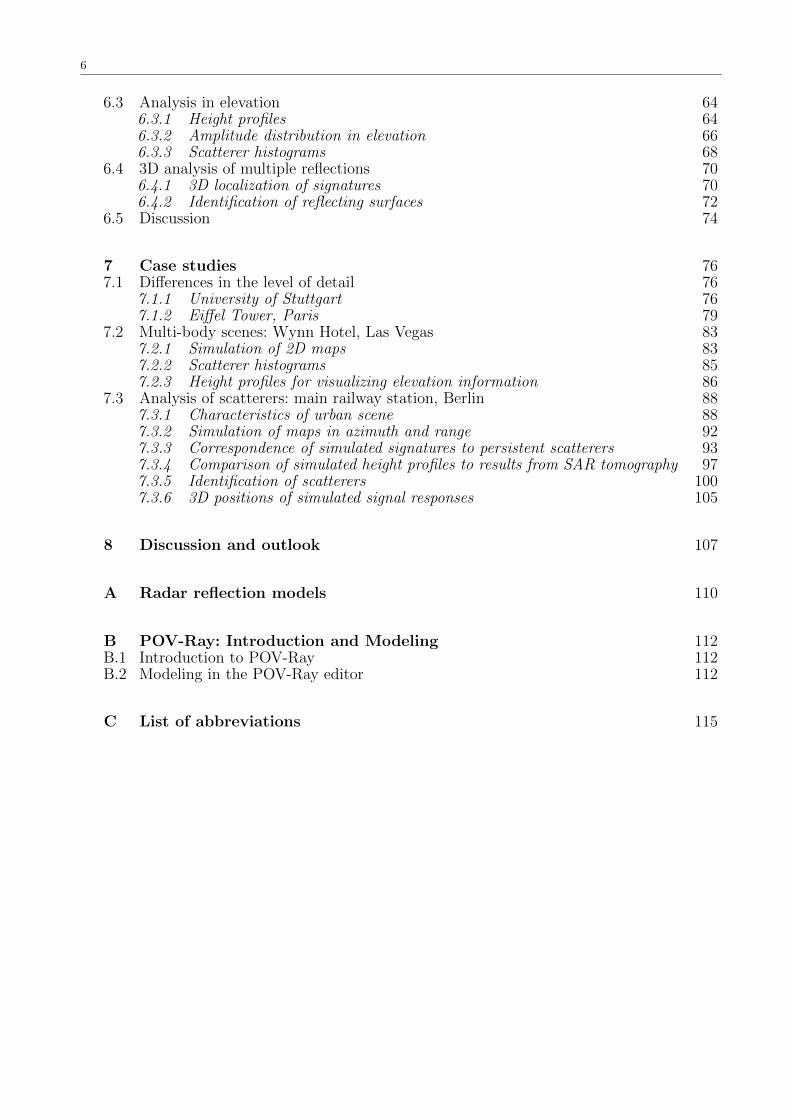
Contents
1 Introduction 71.1 Scientific relevance of the topic 71.2 Objectives and focus 81.3 Reader’s guide 9
2 Basics and state of the art 102.1 Basics on Synthetic Aperture Radar 10
2.1.1 SAR imaging and radar signal 102.1.2 VHR SAR for urban areas 122.1.3 Geometrical distortions in SAR images 132.1.4 SAR image signatures representing buildings 152.1.5 Methods for the localization of scatterers using SAR data 19
2.2 Introduction to render techniques 242.2.1 The render equation 252.2.2 Rendering algorithms 262.2.3 Relevance of render techniques for SAR simulation 28
2.3 SAR simulation - state of the art 292.3.1 Concepts for SAR simulation 292.3.2 VHR SAR simulation for urban areas 312.3.3 Discussion of most related work 31
3 Introduction to RaySAR 343.1 3D SAR simulation approach - new aspects 343.2 Motivation for using POV-Ray 353.3 SAR simulation concept - modeling, sampling, 3D analysis 35
4 Modeling - definition of 3D scenes 374.1 Data sources for 3D building models 374.2 Design of the virtual SAR system 394.3 SAR simulation radiometry 39
4.3.1 Reflection models for SAR simulation 394.3.2 Comparison to radar reflection models 414.3.3 Evaluation of POV Ray reflection models 44
4.4 Modeling step - summary 45
5 Sampling - extraction of data in SAR geometry 475.1 Extraction of geometrical information 47
5.1.1 Detection of reflection contributions 475.1.2 Focusing in azimuth 495.1.3 Focusing in elevation 535.1.4 Detection of specular reflections 55
5.2 Evaluation of the simulation of multiple reflections 555.2.1 Strength of multiple reflected signals 565.2.2 Proportion between multiple reflections and direct backscattering 575.2.3 Geometrical and radiometrical completeness 58
5.3 Sampling step - summary 60
6 Methods for SAR simulation in 3D 626.1 3D models for simulation examples 626.2 Simulation in azimuth and range 62
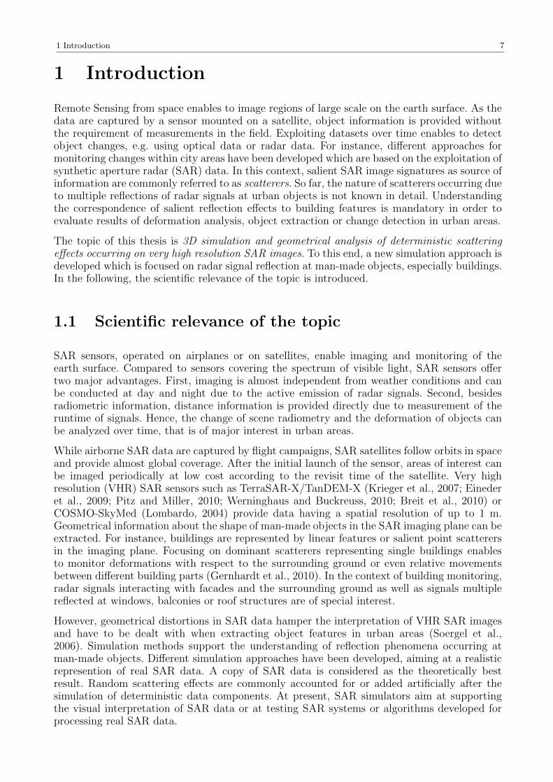
6
6.3 Analysis in elevation 646.3.1 Height profiles 646.3.2 Amplitude distribution in elevation 666.3.3 Scatterer histograms 68
6.4 3D analysis of multiple reflections 706.4.1 3D localization of signatures 706.4.2 Identification of reflecting surfaces 72
6.5 Discussion 74
7 Case studies 767.1 Differences in the level of detail 76
7.1.1 University of Stuttgart 767.1.2 Eiffel Tower, Paris 79
7.2 Multi-body scenes: Wynn Hotel, Las Vegas 837.2.1 Simulation of 2D maps 837.2.2 Scatterer histograms 857.2.3 Height profiles for visualizing elevation information 86
7.3 Analysis of scatterers: main railway station, Berlin 887.3.1 Characteristics of urban scene 887.3.2 Simulation of maps in azimuth and range 927.3.3 Correspondence of simulated signatures to persistent scatterers 937.3.4 Comparison of simulated height profiles to results from SAR tomography 977.3.5 Identification of scatterers 1007.3.6 3D positions of simulated signal responses 105
8 Discussion and outlook 107
A Radar reflection models 110
B POV-Ray: Introduction and Modeling 112B.1 Introduction to POV-Ray 112B.2 Modeling in the POV-Ray editor 112
C List of abbreviations 115
1 Introduction 7
1 Introduction
Remote Sensing from space enables to image regions of large scale on the earth surface. As thedata are captured by a sensor mounted on a satellite, object information is provided withoutthe requirement of measurements in the field. Exploiting datasets over time enables to detectobject changes, e.g. using optical data or radar data. For instance, different approaches formonitoring changes within city areas have been developed which are based on the exploitation ofsynthetic aperture radar (SAR) data. In this context, salient SAR image signatures as source ofinformation are commonly referred to as scatterers. So far, the nature of scatterers occurring dueto multiple reflections of radar signals at urban objects is not known in detail. Understandingthe correspondence of salient reflection effects to building features is mandatory in order toevaluate results of deformation analysis, object extraction or change detection in urban areas.
The topic of this thesis is 3D simulation and geometrical analysis of deterministic scatteringeffects occurring on very high resolution SAR images. To this end, a new simulation approach isdeveloped which is focused on radar signal reflection at man-made objects, especially buildings.In the following, the scientific relevance of the topic is introduced.
1.1 Scientific relevance of the topic
SAR sensors, operated on airplanes or on satellites, enable imaging and monitoring of theearth surface. Compared to sensors covering the spectrum of visible light, SAR sensors offertwo major advantages. First, imaging is almost independent from weather conditions and canbe conducted at day and night due to the active emission of radar signals. Second, besidesradiometric information, distance information is provided directly due to measurement of theruntime of signals. Hence, the change of scene radiometry and the deformation of objects canbe analyzed over time, that is of major interest in urban areas.
While airborne SAR data are captured by flight campaigns, SAR satellites follow orbits in spaceand provide almost global coverage. After the initial launch of the sensor, areas of interest canbe imaged periodically at low cost according to the revisit time of the satellite. Very highresolution (VHR) SAR sensors such as TerraSAR-X/TanDEM-X (Krieger et al., 2007; Einederet al., 2009; Pitz and Miller, 2010; Werninghaus and Buckreuss, 2010; Breit et al., 2010) orCOSMO-SkyMed (Lombardo, 2004) provide data having a spatial resolution of up to 1 m.Geometrical information about the shape of man-made objects in the SAR imaging plane can beextracted. For instance, buildings are represented by linear features or salient point scatterersin the imaging plane. Focusing on dominant scatterers representing single buildings enablesto monitor deformations with respect to the surrounding ground or even relative movementsbetween different building parts (Gernhardt et al., 2010). In the context of building monitoring,radar signals interacting with facades and the surrounding ground as well as signals multiplereflected at windows, balconies or roof structures are of special interest.
However, geometrical distortions in SAR data hamper the interpretation of VHR SAR imagesand have to be dealt with when extracting object features in urban areas (Soergel et al.,2006). Simulation methods support the understanding of reflection phenomena occurring atman-made objects. Different simulation approaches have been developed, aiming at a realisticrepresention of real SAR data. A copy of SAR data is considered as the theoretically bestresult. Random scattering effects are commonly accounted for or added artificially after thesimulation of deterministic data components. At present, SAR simulators aim at supportingthe visual interpretation of SAR data or at testing SAR systems or algorithms developed forprocessing real SAR data.
8 1 Introduction
The analysis of deterministic scatterers on a geometrical basis or the separation of scatterers in2D or 3D has not been realized so far. Hence, the nature of dominant SAR image signatures,which form the basis for the generation of SAR products, is still not known in detail. The SARsimulation approach introduced in this thesis concentrates on this open field of research. De-terministic reflection effects are simulated in three dimensions and methods for supporting theinterpretation and analysis of simulation results are provided. The main goal is to geometricallylink SAR image signatures to the geometry of the corresponding urban objects. In this context,multiple reflected radar signals are expected to cause strong signal responses and, hence, are ofmajor importance.
1.2 Objectives and focus
The development and applications of SAR simulation methods presented in this work are fo-cused on man-made objects imaged by VHR spaceborne SAR sensors. Urban areas or inhabitedareas are of special interest since most methods for exploiting SAR data aim at the detectionof changes affecting human life. Moreover, the number of deterministic SAR image signaturesis expected to be bigger for man-made objects than for areas dominated by vegetation or openfields. The reason is that buildings, bridges, etc. are composed by regular structures such as flatsurfaces, curved surfaces or corners formed by two or three intersecting planes. Thus, the prob-ability of the occurrence of direct backscattering or of multiple reflections at the earth surfaceis assumed to be linked to the regularity of imaged objects. Feature extraction tools designedfor dominant SAR image features are able to separate geometrical or radiometrical informationabout objects from noise. Moreover, the distance information shows higher stability for salientscatterers, offering the possibility to detect deformation in the range of millimeters per yearfrom space. The development of a SAR simulator for analyzing VHR SAR data is mandatoryto understand reflection effects occurring at single objects, now visible in the new generationof SAR data. Basically, there are two major objectives and one minor objective to be fulfilledby the simulation approach:
Objective 1: 3D SAR simulation using object models of high detail
The SAR simulation concept has to be focused on deterministic reflection effects, especiallymultiple reflections. SAR data have to be simulated in three dimensions (azimuth, range, andelevation) using 3D object models characterized by a high level of detail. SAR processingeffects affecting the geometrical position of multiple reflections have to be accounted for. Signalcontributions have to be detected within the simulated scene. Information about the type ofscattering process has to be provided. Eventually, different kinds of reflection effects have to beseparated to enable a directed analysis of scatterers of interest.
Objective 2: Enhancement of knowledge about the nature of scatterers
Besides support for the visual interpretation of SAR data, additional tools for a detailed geo-metrical and quantitative analysis have to be developed in order to enhance knowledge aboutthe nature of scatterers. First, simulation methods have to developed for compensating geomet-rical effects occurring due to the SAR imaging principle. Second, the correspondence of imagesignatures to building features has to be analyzed. To this end, the 3D position of scatterershas to be found within simulated scenes. Finally, the inversion of the SAR imaging process hasto be realized. For that purpose, reflecting surfaces contributing to salient image pixels have tobe identified at simulated object models.
Minor objective 3: Use of existing software packages
Existing software components shall be used for SAR simulation since they are expected to offerreliable, optimized and fast source code libraries as well as progressive simulation algorithms.
1.3 Reader’s guide 9
Furthermore, prominent software packages are anticipated to be maintained for future computerplatforms. Thus, given simulation tools will be adapted to the problem of SAR simulation. Inaddition, essential own developments need to be added in order to provide necessary informationin SAR geometry. Integration of existing methods is expected to save time which can be usedfor realizing the geometrical analysis of scatterers after the simulation of SAR data.
While persuing the objectives, several preconditions and requirements have to be met:
The geometrical correctness of simulation results is more important than the radiometricalcorrectness. Simplified SAR reflection models are anticipated to be sufficient for approximating and an-
alyzing dominant SAR image features. Due to this compromise, integration and simulationof 3D object models of high detail is expected to be feasible. Specular und diffuse reflection of radar signals have to be modeled simultaneously. Random scattering effects are not of major interest and are considered as negligible. Generally, the basic aim is not to provide copies of SAR data but to describe the spatial
distribution of salient image signatures for a given SAR imaging geometry. Deterministicscattering effects of interest may be emphasized when reasonable.
1.3 Reader’s guide
The thesis is structured as follows. Basics on SAR, methods for SAR simulation and renderingtechniques are given in chapter 2. Thereafter, new aspects of the thesis with regard to relatedwork and the concept for SAR simulation are introduced in chapter 3. Requirements for themodeling of scenes are discussed in chapter 4. In this regard, the main focus is on the definitionof object geometries and on reflection properties of surfaces. In chapter 5, the extraction ofgeometrical information in the SAR imaging geometry is explained. Besides, limitations of thesimulator with respect to the detection of signal reflections are discussed. New methods forSAR simulation in three dimensions are introduced in chapter 6. To this end, simulation resultsare presented and discussed for two basic shapes. In chapter 7, simulation results are shownfor different 3D building models and are compared to VHR SAR data. For single buildings andmulti-body scenes, the influence of the level of detail of object models on simulation productsis evaluated. Moreover, simulated data are linked to real data in order to analyze the natureof SAR image signatures. Finally, the results of the thesis and an outlook to future work aregiven in chapter 8.
10 2 Basics and state of the art
2 Basics and state of the art
This chapter covers the relevant theory for the introduction and discussion of the SAR simula-tion approach proposed in this thesis. Basically, two different fields of research are connected:render techniques which are applied for supporting the interpretation of data captured by SARsensors. Fundamental theory corresponding to these fields are introduced in chapters 2.1 and2.2, respectively. Afterward, a literature survey on SAR simulation approaches is given followedby a discussion of related work.
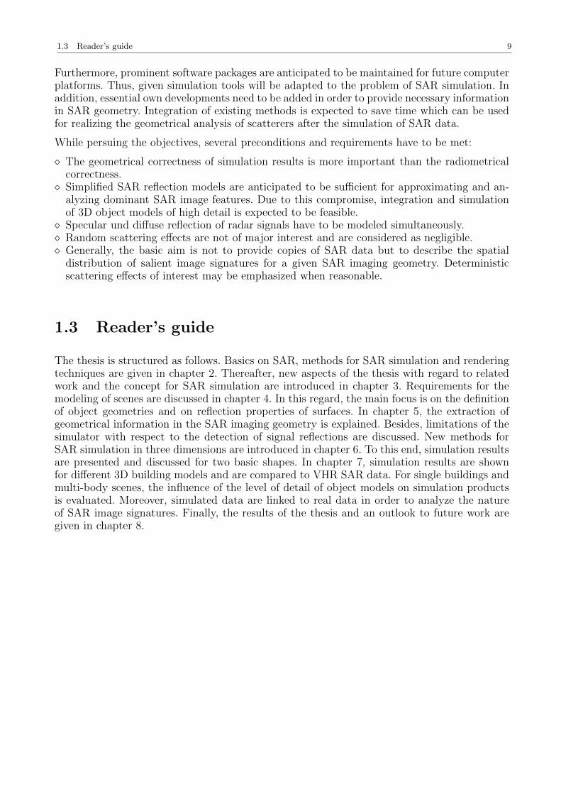
Fig. 1. Imaging geometry of a SAR sensor following its orbit in azimuth direction. The direction of the signal emission(range direction) is defined by look angle θ with respect to the nadir pointing orthogonally to the earth surface. Objectsare imaged within the antenna footprint.
2.1 Basics on Synthetic Aperture Radar
2.1.1 SAR imaging and radar signal
The expression synthetic aperture radar (SAR) characterizes radar systems forming an artifi-cially extended antenna in flight-direction, which are operated airborne or spaceborne. Captur-ing SAR data is independent from day time due to the active emission of signals. Moreover,imaging the earth surface by means of radar signals is almost independent of weather condi-tions, what is a major advantage compared to sensors in the optical or infrared spectrum. In thefollowing, only a brief introduction is given to synthetic aperture radar. Detailed informationabout the functionality of SAR systems can be found in Skolnik (1990), Henderson and Lewis(1998), and Cumming and Wong (2005).
In figure 1, the imaging geometry is shown for a SAR sensor following its orbit. The SAR
2.1 Basics on Synthetic Aperture Radar 11
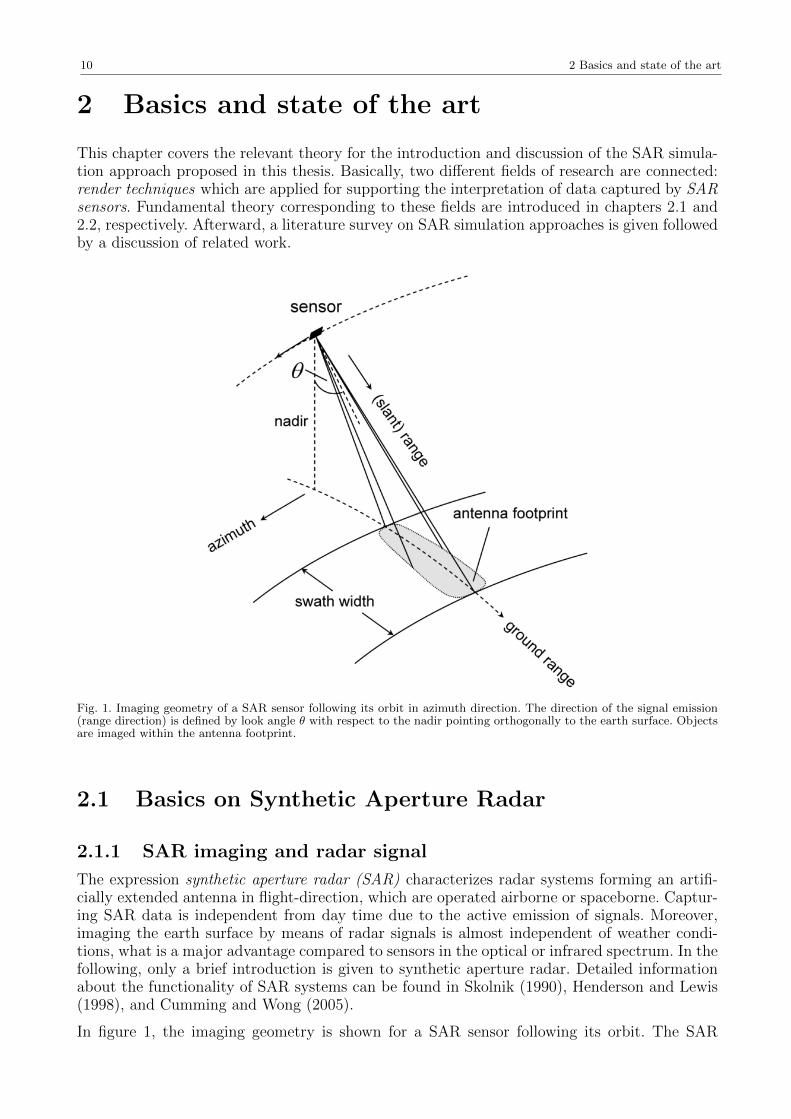
Launch date June 15th, 2007
Antenna size 4.8 m x 0.8 m
Altitude 514km
Inclination 97.44, sun-synchronous
Velocity 7.6km per second
Revisit time 11 days
Range of incidence angle 22 - 55
Scene size 5km in azimuth, 10km in range
Pulse repetition frequency 3000Hz - 6000Hz
Radar center frequency 9.65GHz
Signal wavelength 3.1 cm (X-Band)
Spatial resolution 1.1 m in azimuth, 0.6 m in range
Polarization HH, VV, HV, VH; experimental: full polarization
Table 1. Parameters of the TerraSAR-X satellite.
sensor’s line-of-sight coordinate is called slant range or range. It is commonly located in a planeorthogonal to the flight direction but may also be squinted, i.e. not orthogonal to the line-of-flight. The look angle θ of the SAR sensor with respect to the nadir defines the direction of theline-of sight. In standard SAR imaging mode, called stripmap mode, both the look angle andthe squint angle of the SAR sensor’s line of sight are kept more or less stable. Hence, continuousimaging along the synthetic aperture is enabled what is reasonable for imaging areas of largescale. The local angle of incidence θi at the earth surface corresponds to the angle between theSAR sensor’s line-of-sight to the surface and the normal to the tangent plane at that surface.Electromagnetic signals are emitted in pulsed form expanding in a beam in slant range directionwhich covers the antenna footprint at the earth surface. Signal responses backscattered fromobjects within the antenna footprint are detected at the sensor. In Table 1, the basic systemparameters of the TerraSAR-X satellite are summarized (Eineder et al., 2009; Pitz and Miller,2010; Werninghaus and Buckreuss, 2010; Breit et al., 2010).
The position of a SAR image signature is defined by
the azimuth coordinate x along the orbit the slant range coordinate r captured along the line-of-sight of the SAR sensor
Besides amplitude information giving information about the strength of the backscattered sig-nal, distance information is provided based on measurement of the runtime of the electromag-netic signal. The radar signal can be characterized by
u(τ) = A · exp (j(2πf0τ + Φ)) (1)
where τ is the fast time variable, A is the signal amplitude, j is the imaginary unit, and f0 isthe radar center frequency. The phase Φ for a point scatterer is defined as
Φ = −4π
λR− n · 2π (2)
where R is the spatial distance between the SAR sensor and the imaged object, λ is the signal
12 2 Basics and state of the art
wavelength, and n is an integer keeping Φ within the interval between 0 and 2π. For the sake ofsimplicity, the phase delay caused by the atmosphere as well as phase contributions occurringdue to the scattering of signals on the earth surface are neglected. The signal intensity I isderived by squaring the amplitude A, i.e. I = A2. Being related to the frequency of the carriersignal, the signal wavelength is
λ =c
f0
(3)
where c is the velocity of light. SAR wave signals are emitted either in horizontal or in verticalpolarization and are detected in horizontal and/or vertical polarization (see e.g. Tsang andKong (2001) for further information about the polarization of radar signals). For example,TerraSAR-X covers the combinations HH, i.e. emission and detection of horizontal polarizedradar signals, VV, HV and VH in standard mode (see Table 1).
The measurement of the signal runtime in slant range direction is enabled by emitting achirp, whose signal power is temporally distributed. During post-processing of the SAR rawdata (Bamler, 1992; Franceschetti and Lanari, 1999), the signal power is regained by correlatingthe received signal with a reference chirp in range. For instance, the processed signal responseof a corner reflector is a sinc-function. In theory, the width of the sinc-function’s main lobedetermines the resolution in range and is
δr =c
2fr(4)
where fr is the bandwidth of the chirp emitted by the radar antenna.
In azimuth direction, objects at the earth surface are imaged coherently by a synthetic antenna.To this end, the motion of the platform is utilized for collecting SAR raw data of a target overa short time period. The signal power in azimuth is regained by correlation of the SAR rawdata with a reference chirp in azimuth. Comparable to the range domain, the signal responseof a corner reflector yields a sinc function whose mainlobe width defines the spatial resolutionof the SAR system in azimuth:
δx =L
2(5)
where L is the physical length of the radar antenna.
SAR systems operated in spotlight mode reach a spatial resolution in azimuth which is higherthan the theoretical limit given by equation 5. The length of the synthetic aperture is increasedby squinting the radar beam in direction to the area to be imaged. Thereby, the target band-width in azimuth becomes larger than in standard stripmap mode. In case of TerraSAR-X, thespatial resolution in azimuth is improved from 3.3 m in stripmap mode to 1.1 m in high reso-lution spotlight mode (see Table 1). As major drawback of spotlight mode, continuous imagingof the earth surface is not possible. Hence, the area of interest has to be defined a-priori.
2.1.2 VHR SAR for urban areas
When imaged by SAR sensors of lower resolution, e.g. ERS-1/2 (Attema et al., 1998) or En-visat (Louet and Bruzzi, 1999), man-made objects are included in a low number of resolutioncells. Hence, monitoring of objects of interest such as residental buildings, industrial buildings,bridges, etc. is limited or even impossible. For instance, in Perski et al. (2007) the collapse oflarge buildings is analyzed based on distance information corresponding to salient point signa-tures. To this end, data stacks of the ERS-1/2 and Envisat satellite missions are processed using
2.1 Basics on Synthetic Aperture Radar 13
Persistent Scatterer Interferometry (see chapter 2.1.5). However, the detection of deformationsignals at buildings is limited by the low number of point signatures representing the objectsof interest.
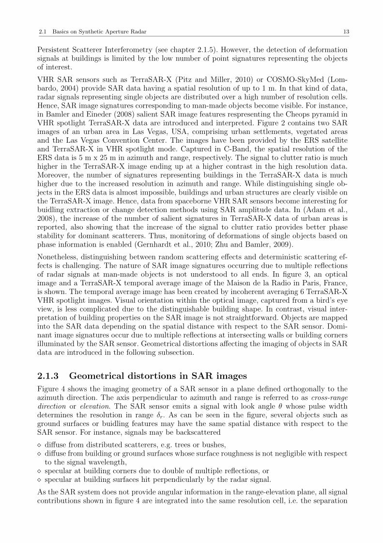
VHR SAR sensors such as TerraSAR-X (Pitz and Miller, 2010) or COSMO-SkyMed (Lom-bardo, 2004) provide SAR data having a spatial resolution of up to 1 m. In that kind of data,radar signals representing single objects are distributed over a high number of resolution cells.Hence, SAR image signatures corresponding to man-made objects become visible. For instance,in Bamler and Eineder (2008) salient SAR image features respresenting the Cheops pyramid inVHR spotlight TerraSAR-X data are introduced and interpreted. Figure 2 contains two SARimages of an urban area in Las Vegas, USA, comprising urban settlements, vegetated areasand the Las Vegas Convention Center. The images have been provided by the ERS satelliteand TerraSAR-X in VHR spotlight mode. Captured in C-Band, the spatial resolution of theERS data is 5 m x 25 m in azimuth and range, respectively. The signal to clutter ratio is muchhigher in the TerraSAR-X image ending up at a higher contrast in the high resolution data.Moreover, the number of signatures representing buildings in the TerraSAR-X data is muchhigher due to the increased resolution in azimuth and range. While distinguishing single ob-jects in the ERS data is almost impossible, buildings and urban structures are clearly visible onthe TerraSAR-X image. Hence, data from spaceborne VHR SAR sensors become interesting forbuidling extraction or change detection methods using SAR amplitude data. In (Adam et al.,2008), the increase of the number of salient signatures in TerraSAR-X data of urban areas isreported, also showing that the increase of the signal to clutter ratio provides better phasestability for dominant scatterers. Thus, monitoring of deformations of single objects based onphase information is enabled (Gernhardt et al., 2010; Zhu and Bamler, 2009).
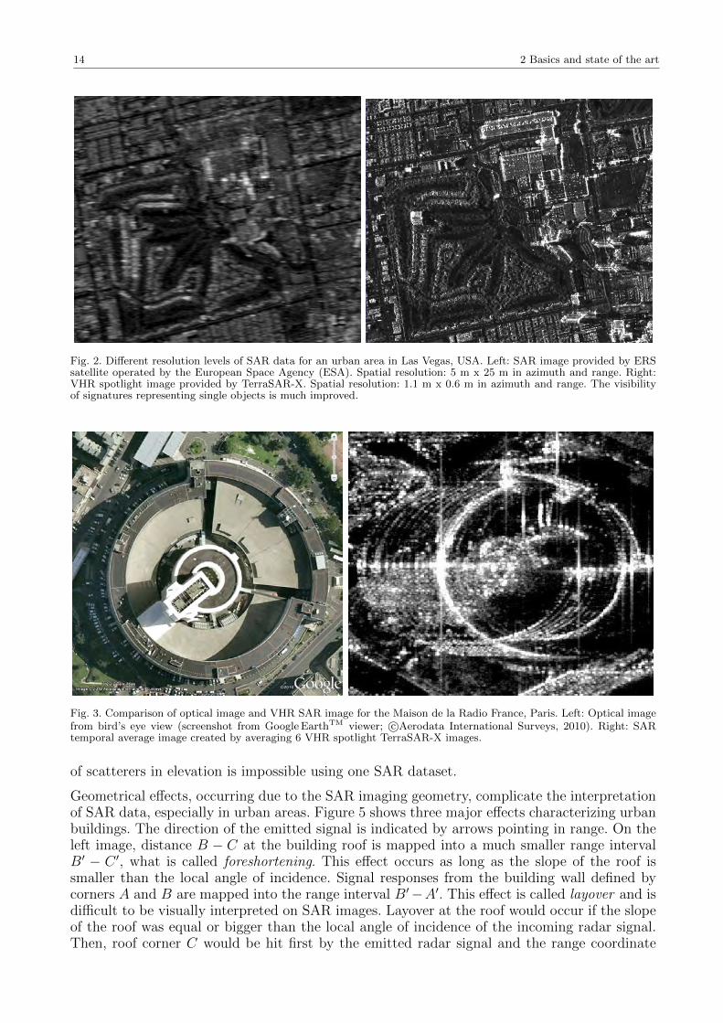
Nonetheless, distinguishing between random scattering effects and deterministic scattering ef-fects is challenging. The nature of SAR image signatures occurring due to multiple reflectionsof radar signals at man-made objects is not understood to all ends. In figure 3, an opticalimage and a TerraSAR-X temporal average image of the Maison de la Radio in Paris, France,is shown. The temporal average image has been created by incoherent averaging 6 TerraSAR-XVHR spotlight images. Visual orientation within the optical image, captured from a bird’s eyeview, is less complicated due to the distinguishable building shape. In contrast, visual inter-pretation of building properties on the SAR image is not straightforward. Objects are mappedinto the SAR data depending on the spatial distance with respect to the SAR sensor. Domi-nant image signatures occur due to multiple reflections at intersecting walls or building cornersilluminated by the SAR sensor. Geometrical distortions affecting the imaging of objects in SARdata are introduced in the following subsection.
2.1.3 Geometrical distortions in SAR images
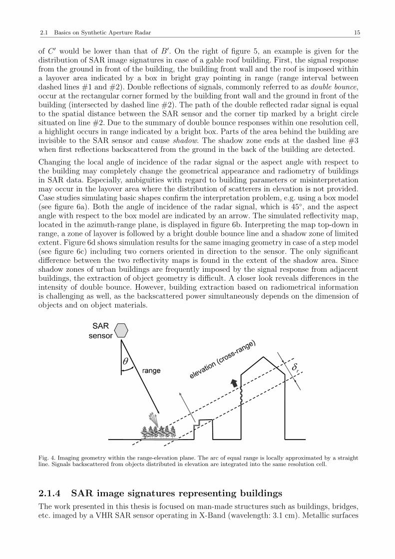
Figure 4 shows the imaging geometry of a SAR sensor in a plane defined orthogonally to theazimuth direction. The axis perpendicular to azimuth and range is referred to as cross-rangedirection or elevation. The SAR sensor emits a signal with look angle θ whose pulse widthdetermines the resolution in range δr. As can be seen in the figure, several objects such asground surfaces or buidling features may have the same spatial distance with respect to theSAR sensor. For instance, signals may be backscattered
diffuse from distributed scatterers, e.g. trees or bushes, diffuse from building or ground surfaces whose surface roughness is not negligible with respect
to the signal wavelength, specular at building corners due to double of multiple reflections, or specular at building surfaces hit perpendicularly by the radar signal.
As the SAR system does not provide angular information in the range-elevation plane, all signalcontributions shown in figure 4 are integrated into the same resolution cell, i.e. the separation
14 2 Basics and state of the art
Fig. 2. Different resolution levels of SAR data for an urban area in Las Vegas, USA. Left: SAR image provided by ERSsatellite operated by the European Space Agency (ESA). Spatial resolution: 5 m x 25 m in azimuth and range. Right:VHR spotlight image provided by TerraSAR-X. Spatial resolution: 1.1 m x 0.6 m in azimuth and range. The visibilityof signatures representing single objects is much improved.
Fig. 3. Comparison of optical image and VHR SAR image for the Maison de la Radio France, Paris. Left: Optical imagefrom bird’s eye view (screenshot from Google EarthTM viewer; c©Aerodata International Surveys, 2010). Right: SARtemporal average image created by averaging 6 VHR spotlight TerraSAR-X images.
of scatterers in elevation is impossible using one SAR dataset.
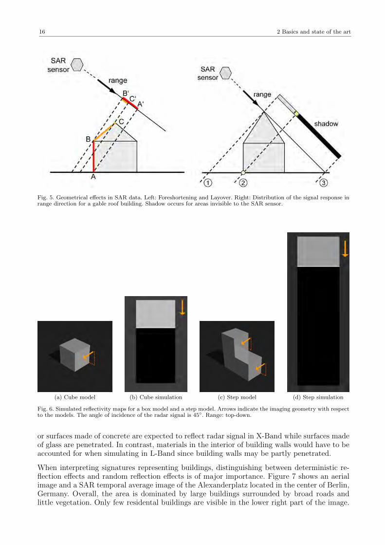
Geometrical effects, occurring due to the SAR imaging geometry, complicate the interpretationof SAR data, especially in urban areas. Figure 5 shows three major effects characterizing urbanbuildings. The direction of the emitted signal is indicated by arrows pointing in range. On theleft image, distance B − C at the building roof is mapped into a much smaller range intervalB′ − C ′, what is called foreshortening. This effect occurs as long as the slope of the roof issmaller than the local angle of incidence. Signal responses from the building wall defined bycorners A and B are mapped into the range interval B′−A′. This effect is called layover and isdifficult to be visually interpreted on SAR images. Layover at the roof would occur if the slopeof the roof was equal or bigger than the local angle of incidence of the incoming radar signal.Then, roof corner C would be hit first by the emitted radar signal and the range coordinate
2.1 Basics on Synthetic Aperture Radar 15
of C ′ would be lower than that of B′. On the right of figure 5, an example is given for thedistribution of SAR image signatures in case of a gable roof building. First, the signal responsefrom the ground in front of the building, the building front wall and the roof is imposed withina layover area indicated by a box in bright gray pointing in range (range interval betweendashed lines #1 and #2). Double reflections of signals, commonly referred to as double bounce,occur at the rectangular corner formed by the building front wall and the ground in front of thebuilding (intersected by dashed line #2). The path of the double reflected radar signal is equalto the spatial distance between the SAR sensor and the corner tip marked by a bright circlesituated on line #2. Due to the summary of double bounce responses within one resolution cell,a highlight occurs in range indicated by a bright box. Parts of the area behind the building areinvisible to the SAR sensor and cause shadow. The shadow zone ends at the dashed line #3when first reflections backscattered from the ground in the back of the building are detected.
Changing the local angle of incidence of the radar signal or the aspect angle with respect tothe building may completely change the geometrical appearance and radiometry of buildingsin SAR data. Especially, ambiguities with regard to building parameters or misinterpretationmay occur in the layover area where the distribution of scatterers in elevation is not provided.Case studies simulating basic shapes confirm the interpretation problem, e.g. using a box model(see figure 6a). Both the angle of incidence of the radar signal, which is 45, and the aspectangle with respect to the box model are indicated by an arrow. The simulated reflectivity map,located in the azimuth-range plane, is displayed in figure 6b. Interpreting the map top-down inrange, a zone of layover is followed by a bright double bounce line and a shadow zone of limitedextent. Figure 6d shows simulation results for the same imaging geometry in case of a step model(see figure 6c) including two corners oriented in direction to the sensor. The only significantdifference between the two reflectivity maps is found in the extent of the shadow area. Sinceshadow zones of urban buildings are frequently imposed by the signal response from adjacentbuildings, the extraction of object geometry is difficult. A closer look reveals differences in theintensity of double bounce. However, building extraction based on radiometrical informationis challenging as well, as the backscattered power simultaneously depends on the dimension ofobjects and on object materials.
Fig. 4. Imaging geometry within the range-elevation plane. The arc of equal range is locally approximated by a straightline. Signals backscattered from objects distributed in elevation are integrated into the same resolution cell.
2.1.4 SAR image signatures representing buildings
The work presented in this thesis is focused on man-made structures such as buildings, bridges,etc. imaged by a VHR SAR sensor operating in X-Band (wavelength: 3.1 cm). Metallic surfaces
16 2 Basics and state of the art
Fig. 5. Geometrical effects in SAR data. Left: Foreshortening and Layover. Right: Distribution of the signal response inrange direction for a gable roof building. Shadow occurs for areas invisible to the SAR sensor.
(a) Cube model (b) Cube simulation (c) Step model (d) Step simulation
Fig. 6. Simulated reflectivity maps for a box model and a step model. Arrows indicate the imaging geometry with respectto the models. The angle of incidence of the radar signal is 45. Range: top-down.
or surfaces made of concrete are expected to reflect radar signal in X-Band while surfaces madeof glass are penetrated. In contrast, materials in the interior of building walls would have to beaccounted for when simulating in L-Band since building walls may be partly penetrated.
When interpreting signatures representing buildings, distinguishing between deterministic re-flection effects and random reflection effects is of major importance. Figure 7 shows an aerialimage and a SAR temporal average image of the Alexanderplatz located in the center of Berlin,Germany. Overall, the area is dominated by large buildings surrounded by broad roads andlittle vegetation. Only few residental buildings are visible in the lower right part of the image.
2.1 Basics on Synthetic Aperture Radar 17
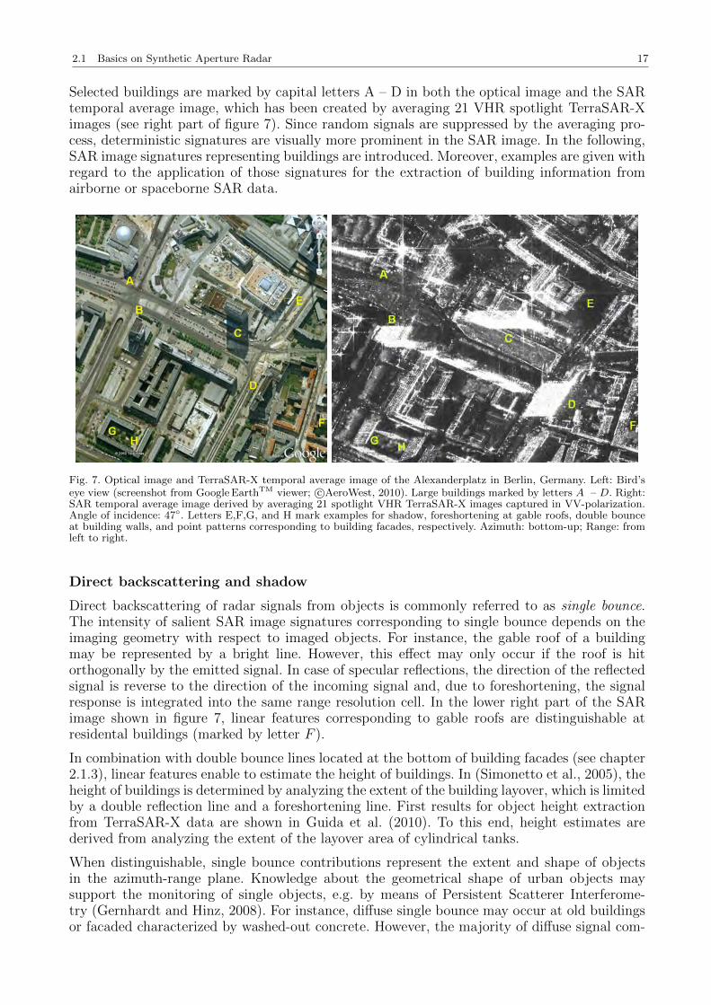
Selected buildings are marked by capital letters A – D in both the optical image and the SARtemporal average image, which has been created by averaging 21 VHR spotlight TerraSAR-Ximages (see right part of figure 7). Since random signals are suppressed by the averaging pro-cess, deterministic signatures are visually more prominent in the SAR image. In the following,SAR image signatures representing buildings are introduced. Moreover, examples are given withregard to the application of those signatures for the extraction of building information fromairborne or spaceborne SAR data.
Fig. 7. Optical image and TerraSAR-X temporal average image of the Alexanderplatz in Berlin, Germany. Left: Bird’seye view (screenshot from Google EarthTM viewer; c©AeroWest, 2010). Large buildings marked by letters A – D. Right:SAR temporal average image derived by averaging 21 spotlight VHR TerraSAR-X images captured in VV-polarization.Angle of incidence: 47. Letters E,F,G, and H mark examples for shadow, foreshortening at gable roofs, double bounceat building walls, and point patterns corresponding to building facades, respectively. Azimuth: bottom-up; Range: fromleft to right.
Direct backscattering and shadow
Direct backscattering of radar signals from objects is commonly referred to as single bounce.The intensity of salient SAR image signatures corresponding to single bounce depends on theimaging geometry with respect to imaged objects. For instance, the gable roof of a buildingmay be represented by a bright line. However, this effect may only occur if the roof is hitorthogonally by the emitted signal. In case of specular reflections, the direction of the reflectedsignal is reverse to the direction of the incoming signal and, due to foreshortening, the signalresponse is integrated into the same range resolution cell. In the lower right part of the SARimage shown in figure 7, linear features corresponding to gable roofs are distinguishable atresidental buildings (marked by letter F ).
In combination with double bounce lines located at the bottom of building facades (see chapter2.1.3), linear features enable to estimate the height of buildings. In (Simonetto et al., 2005), theheight of buildings is determined by analyzing the extent of the building layover, which is limitedby a double reflection line and a foreshortening line. First results for object height extractionfrom TerraSAR-X data are shown in Guida et al. (2010). To this end, height estimates arederived from analyzing the extent of the layover area of cylindrical tanks.
When distinguishable, single bounce contributions represent the extent and shape of objectsin the azimuth-range plane. Knowledge about the geometrical shape of urban objects maysupport the monitoring of single objects, e.g. by means of Persistent Scatterer Interferome-try (Gernhardt and Hinz, 2008). For instance, diffuse single bounce may occur at old buildingsor facaded characterized by washed-out concrete. However, the majority of diffuse signal com-
18 2 Basics and state of the art
ponents backscattered from buildings may be hardly visible in SAR data since most buildingwalls show little roughness compared to the signal wavelength. Moreover, diffuse signals frombuilding walls may be overlayed by diffuse backscatter from the ground in front of the building.
The exploitation of shadow provides information about the height of buildings. In figure 7, letterE in the SAR image marks an example for shadow at buildings. For instance, the height ofbuilding walls invisible to the SAR sensor can be estimated by analyzing the length of buildingshadows (Bolter and Leberl, 2000). Hill et al. (2006) vary parameters of a 2.5D building modeland map it into the azimuth-range plane for comparison with airborne SAR data. Afterwards,the building parameters are optimized by cross-checking the extent of the building shadow byan active-contour library.
Double reflections
Linear double bounce signatures occur, for instance, in case of signal interaction with facadesand the surrounding ground. Ideal corners provoking double bounce are commonly referred to asdihedrals and consist of two surfaces oriented orthogonally to each other. A double bounce lineshows strong intensity if the dihedral faces the line-of-sight of the SAR sensor. Hence, buildingsfacades oriented in line-of-flight of the SAR sensor are likely to cause dominant signatures. Inthe SAR temporal average image shown in figure 7, a double bounce line is marked by letter G.In Brunner et al. (2009), the power of double bounce response from building walls is analyzeddepending on the aspect angle. Complementary, the geometry of linear signatures correspondingto signals interacting with building walls and the surrounding ground is extracted and discussedin Wegner et al. (2010).
As reported in the literature, double bounce lines occuring in SAR data of urban areas are usedfor extracting the outline of buildings. In Quartulli and Datcu (2004), the shape of buildings isextracted in the azimuth-range plane from single airborne SAR data, what is performed basedon Monte Carlo simulation. Besides other image features, double reflection lines are analyzedfor finding the best fit for building parameters. By fusing salient double bounce lines extractedfrom SAR data captured from orthogonal aspect angles, the detection rate of buildings and thecorrectness of the extraction of rectangular building outlines can be increased (Thiele et al.,2007b; Xu and Jin, 2007).
Besides geometrical information about the shape of buildings, dominant double bounce linesenable the detection of building heights based on SAR image radiometry. Franceschetti et al.(2007) present a functional model for estimating the height of buildings, characterized by flatroofs, from airborne SAR data based on the intensity of double bounce lines. In order to focuson the influence of object geometry, knowledge about surface materials is necessary. Guida et al.(2010) show first results of object height extraction based on the radiometry of TerraSAR-Xdata captured in stripmap or spotlight mode.
Triple reflections
The majority of modern buildings within urban areas show regular shapes including corners.Ideal corner reflectors, commonly referred to as trihedrals, are composed by three orthogonalplanes. In case of an ideal corner roughly oriented in line-of-sight of the SAR sensor, a salientpoint signature is likely to appear on the SAR image, whose intensity is characterized by a2D − sinc-function. In Groot and Otten (1993), it is shown that the signal peak of a cornerreflector is always located within one resolution cell even if the size of a corner reflector is largerthan the resolution of the SAR system. The effective surface contributing to the radar signalresponse of a corner reflector, oriented in line-of-sight of the SAR sensor, forms a pentagonalshape (Sarabandi and Chiu, 1996). In figure 7, facades in the SAR temporal average image aredominated by point signatures organized in patterns. As an example, letter H marks a pointpattern which is likely to be linked to trihedral reflections of radar signals.
2.1 Basics on Synthetic Aperture Radar 19
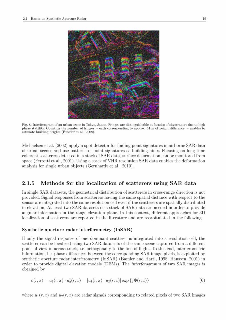
Fig. 8. Interferogram of an urban scene in Tokyo, Japan. Fringes are distinguishable at facades of skyscrapers due to highphase stability. Counting the number of fringes – each corresponding to approx. 44 m of height difference – enables toestimate building heights (Eineder et al., 2008).
Michaelsen et al. (2002) apply a spot detector for finding point signatures in airborne SAR dataof urban scenes and use patterns of point signatures as building hints. Focusing on long-timecoherent scatterers detected in a stack of SAR data, surface deformation can be monitored fromspace (Ferretti et al., 2001). Using a stack of VHR resolution SAR data enables the deformationanalysis for single urban objects (Gernhardt et al., 2010).
2.1.5 Methods for the localization of scatterers using SAR data
In single SAR datasets, the geometrical distribution of scatterers in cross-range direction is notprovided. Signal responses from scatterers having the same spatial distance with respect to thesensor are integrated into the same resolution cell even if the scatterers are spatially distributedin elevation. At least two SAR datasets or a stack of SAR data are needed in order to provideangular information in the range-elevation plane. In this context, different approaches for 3Dlocalization of scatterers are reported in the literature and are recapitulated in the following.
Synthetic aperture radar interferometry (InSAR)
If only the signal response of one dominant scatterer is integrated into a resolution cell, thescatterer can be localized using two SAR data sets of the same scene captured from a differentpoint of view in across-track, i.e. orthogonally to the line-of-flight. To this end, interferometricinformation, i.e. phase differences between the corresponding SAR image pixels, is exploited bysynthetic aperture radar interferometry (InSAR) (Bamler and Hartl, 1998; Hanssen, 2001) inorder to provide digital elevation models (DEMs). The interferogramm of two SAR images isobtained by
υ(r, x) = u1(r, x) · u∗2(r, x) = |u1(r, x)| |u2(r, x)| exp jΦ(r, x) (6)
where u1(r, x) and u2(r, x) are radar signals corresponding to related pixels of two SAR images
20 2 Basics and state of the art
imaging the same area of interest. The interferometric phase is defined by
Φ(r, x) =4π
λ∆R (7)
and is ambiguous with respect to integer multiples of 2π. The sensibility of the phase dependson the signal wavelength λ as well as on the range difference ∆R = R2 −R1 where R1 and R2
are the spatial distances between the two sensor positions and the target, respectively.
In figure 8, the interferometric phase is shown for an urban scene in Tokyo, Japan. The SARdata have been captured by TerraSAR-X in spotlight mode. Detailed information can be foundin Eineder et al. (2008) and Eineder et al. (2009). The interferometric phase has been obtainedfrom two subsequent passes of the SAR sensor and is represented by a color wheel continuouslychanging between red, green and blue. Turning the color wheel from red to red correspondsto a phase difference of 2π which is referred to as a fringe. For the example at hand, fringesare clearly distinguishable at the facades of skyscrapers in the interferogram due to high phasestability.
The height of the building can be estimated by unwrapping the interferometric phase in orderto get the absolute phase with respect to a reference point selected within the urban scene. Forinstance, Bolter and Leberl (2000) extract 2.5D building models from multi-aspect airborneInSAR data. The height of building facades visible to the SAR sensor is estimated based oninterferometric information. Gamba et al. (2000) fit horizontal planes to 3D surface informationprovided by airborne InSAR data in order to estimate the height of buildings. To this end, scanlines are defined in range direction and are used as seeds in an iterative region growing processfor the detection of flat regions.
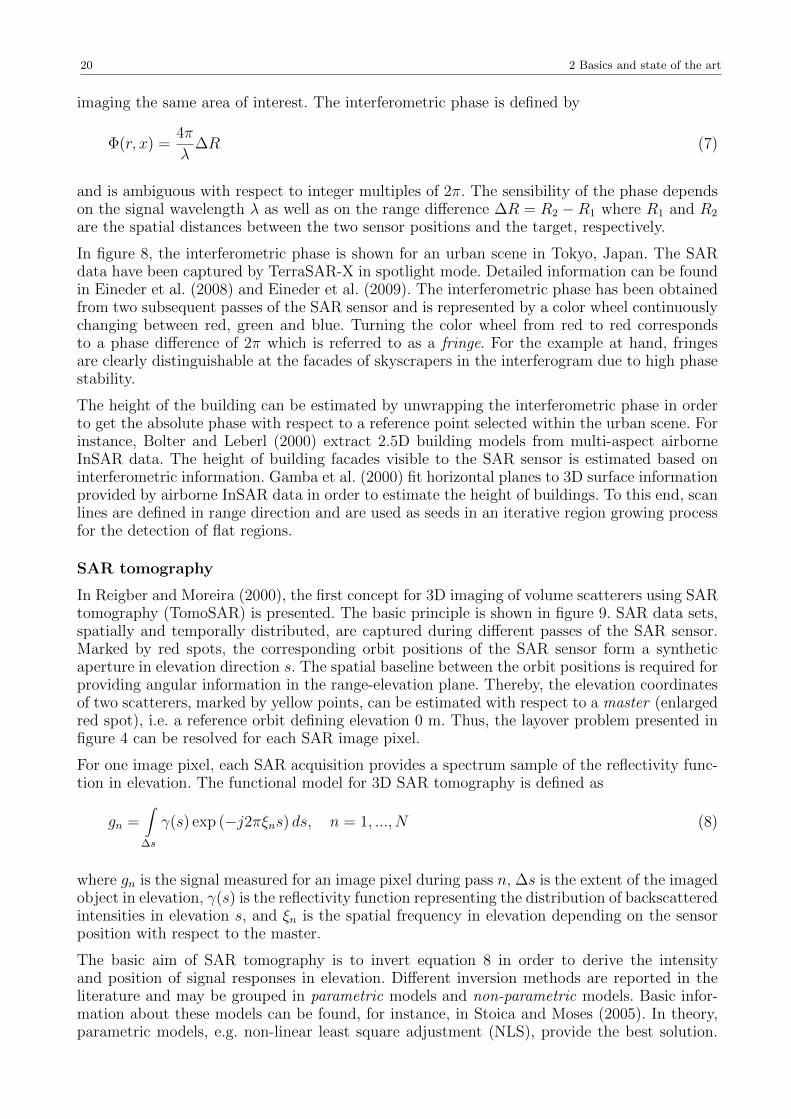
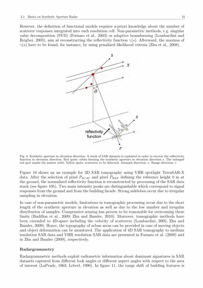
SAR tomography
In Reigber and Moreira (2000), the first concept for 3D imaging of volume scatterers using SARtomography (TomoSAR) is presented. The basic principle is shown in figure 9. SAR data sets,spatially and temporally distributed, are captured during different passes of the SAR sensor.Marked by red spots, the corresponding orbit positions of the SAR sensor form a syntheticaperture in elevation direction s. The spatial baseline between the orbit positions is required forproviding angular information in the range-elevation plane. Thereby, the elevation coordinatesof two scatterers, marked by yellow points, can be estimated with respect to a master (enlargedred spot), i.e. a reference orbit defining elevation 0 m. Thus, the layover problem presented infigure 4 can be resolved for each SAR image pixel.
For one image pixel, each SAR acquisition provides a spectrum sample of the reflectivity func-tion in elevation. The functional model for 3D SAR tomography is defined as
gn =∫
∆s
γ(s) exp (−j2πξns) ds, n = 1, ..., N (8)
where gn is the signal measured for an image pixel during pass n, ∆s is the extent of the imagedobject in elevation, γ(s) is the reflectivity function representing the distribution of backscatteredintensities in elevation s, and ξn is the spatial frequency in elevation depending on the sensorposition with respect to the master.
The basic aim of SAR tomography is to invert equation 8 in order to derive the intensityand position of signal responses in elevation. Different inversion methods are reported in theliterature and may be grouped in parametric models and non-parametric models. Basic infor-mation about these models can be found, for instance, in Stoica and Moses (2005). In theory,parametric models, e.g. non-linear least square adjustment (NLS), provide the best solution.
2.1 Basics on Synthetic Aperture Radar 21
However, the definition of functional models requires a-priori knowledge about the number ofscatterer responses integrated into each resolution cell. Non-parametric methods, e.g. singularvalue decomposition (SVD) (Fornaro et al., 2003) or adaptive beamforming (Lombardini andReigber, 2003), aim at reconstructing the reflectivity function γ(s). Afterward, the maxima ofγ(s) have to be found, for instance, by using penalized likelihood criteria (Zhu et al., 2008).
Fig. 9. Synthetic aperture in elevation direction. A stack of SAR datasets is exploited in order to recover the reflectivityfunction in elevation direction. Red spots: orbits forming the synthetic aperture in elevation direction s. The enlargedred spot marks the master orbit. Yellow spots: scatterers to be detected. Azimuth direction: x. Range direction: r.
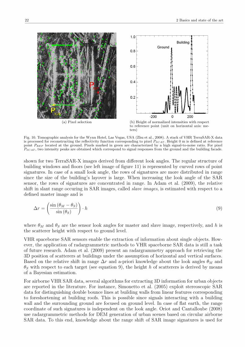
Figure 10 shows an an example for 3D SAR tomography using VHR spotlight TerraSAR-Xdata. After the selection of pixel PSCAT and pixel PREF defining the reference height 0 m atthe ground, the normalized reflectivity function is reconstructed by processing of the SAR datastack (see figure 10b). Two main intensity peaks are distinguishable which correspond to signalresponses from the ground and from the building facade. Strong sidelobes occur due to irregularsampling in elevation.
In case of non-parametric models, limitations in tomographic processing occur due to the shortlength of the synthetic aperture in elevation as well as due to the low number and irregulardistribution of samples. Compressive sensing has proven to be reasonable for overcoming theselimits (Budillon et al., 2009; Zhu and Bamler, 2010). Moreover, tomographic methods havebeen extended to 4D-space including the velocity of scatterers (Lombardini, 2005; Zhu andBamler, 2009). Hence, the topography of urban areas can be provided in case of moving objectsand object deformation can be monitored. The application of 4D SAR tomography to mediumresolution SAR data and VHR resolution SAR data are presented in Fornaro et al. (2009) andin Zhu and Bamler (2009), respectively.
Radargrammetry
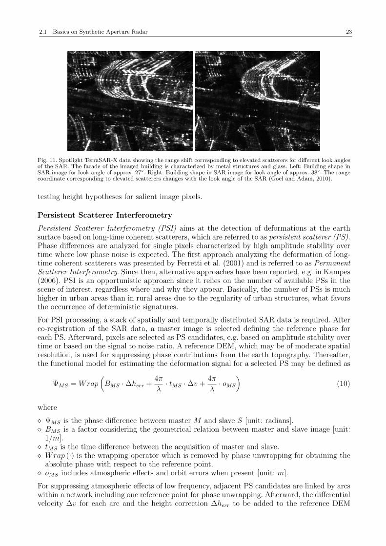
Radargrammetric methods exploit radiometric information about dominant signatures in SARdatasets captured from different look angles or different aspect angles with respect to the areaof interest (LaPrade, 1963; Leberl, 1990). In figure 11, the range shift of building features is
22 2 Basics and state of the art
(a) Pixel selection (b) Height of normalized intensities with respectto reference point (unit on horizontal axis: me-ters)
Fig. 10. Tomographic analysis for the Wynn Hotel, Las Vegas, USA (Zhu et al., 2008). A stack of VHR TerraSAR-X datais processed for reconstructing the reflectivity function corresponding to pixel PSCAT . Height 0 m is defined at referencepoint PREF located at the ground. Pixels marked in green are characterized by a high signal-to-noise ratio. For pixelPSCAT , two intensity peaks are obtained which correspond to signal responses from the ground and the building facade.
shown for two TerraSAR-X images derived from different look angles. The regular structure ofbuilding windows and floors (see left image of figure 11) is represented by curved rows of pointsignatures. In case of a small look angle, the rows of signatures are more distributed in rangesince the size of the building’s layover is large. When increasing the look angle of the SARsensor, the rows of signatures are concentrated in range. In Adam et al. (2009), the relativeshift in slant range occuring in SAR images, called slave images, is estimated with respect to adefined master image and is
∆r =
(sin (θM − θS)
sin (θS)
)· h (9)
where θM and θS are the sensor look angles for master and slave image, respectively, and h isthe scatterer height with respect to ground level.
VHR spaceborne SAR sensors enable the extraction of information about single objects. How-ever, the application of radargrammetric methods to VHR spaceborne SAR data is still a taskof future research. Adam et al. (2009) present an radargrammetry approach for retrieving the3D position of scatterers at buildings under the assumption of horizontal and vertical surfaces.Based on the relative shift in range ∆r and a-priori knowledge about the look angles θM andθS with respect to each target (see equation 9), the height h of scatterers is derived by meansof a Bayesian estimation.
For airborne VHR SAR data, several algorithms for extracting 3D information for urban objectsare reported in the literature. For instance, Simonetto et al. (2005) exploit stereoscopic SARdata for distinguishing double bounce lines at building walls from linear features correspondingto foreshortening at building roofs. This is possible since signals interacting with a buildingwall and the surrounding ground are focused on ground level. In case of flat earth, the rangecoordinate of such signatures is independent on the look angle. Oriot and Cantalloube (2008)use radargrammetric methods for DEM generation of urban scenes based on circular airborneSAR data. To this end, knowledge about the range shift of SAR image signatures is used for
2.1 Basics on Synthetic Aperture Radar 23
Fig. 11. Spotlight TerraSAR-X data showing the range shift corresponding to elevated scatterers for different look anglesof the SAR. The facade of the imaged building is characterized by metal structures and glass. Left: Building shape inSAR image for look angle of approx. 27. Right: Building shape in SAR image for look angle of approx. 38. The rangecoordinate corresponding to elevated scatterers changes with the look angle of the SAR (Goel and Adam, 2010).
testing height hypotheses for salient image pixels.
Persistent Scatterer Interferometry
Persistent Scatterer Interferometry (PSI) aims at the detection of deformations at the earthsurface based on long-time coherent scatterers, which are referred to as persistent scatterer (PS).Phase differences are analyzed for single pixels characterized by high amplitude stability overtime where low phase noise is expected. The first approach analyzing the deformation of long-time coherent scatterers was presented by Ferretti et al. (2001) and is referred to as PermanentScatterer Interferometry. Since then, alternative approaches have been reported, e.g. in Kampes(2006). PSI is an opportunistic approach since it relies on the number of available PSs in thescene of interest, regardless where and why they appear. Basically, the number of PSs is muchhigher in urban areas than in rural areas due to the regularity of urban structures, what favorsthe occurrence of deterministic signatures.
For PSI processing, a stack of spatially and temporally distributed SAR data is required. Afterco-registration of the SAR data, a master image is selected defining the reference phase foreach PS. Afterward, pixels are selected as PS candidates, e.g. based on amplitude stability overtime or based on the signal to noise ratio. A reference DEM, which may be of moderate spatialresolution, is used for suppressing phase contributions from the earth topography. Thereafter,the functional model for estimating the deformation signal for a selected PS may be defined as
ΨMS = Wrap(BMS ·∆herr +
4π
λ· tMS ·∆v +
4π
λ· oMS
)(10)
where
ΨMS is the phase difference between master M and slave S [unit: radians]. BMS is a factor considering the geometrical relation between master and slave image [unit:
1/m]. tMS is the time difference between the acquisition of master and slave. Wrap (·) is the wrapping operator which is removed by phase unwrapping for obtaining the
absolute phase with respect to the reference point. oMS includes atmospheric effects and orbit errors when present [unit: m].
For suppressing atmospheric effects of low frequency, adjacent PS candidates are linked by arcswithin a network including one reference point for phase unwrapping. Afterward, the differentialvelocity ∆v for each arc and the height correction ∆herr to be added to the reference DEM
24 2 Basics and state of the art
can be estimated based on statistical assumptions. However, there are two major limitations.First, a deformation model has to be defined in order to separate the deformation signal fromatmospheric residuals and noise. Second, the separation of scatterers within the same resolutioncell is not possible. A theoretical concept for overcoming the second limitation is reportedin Ferretti et al. (2005).
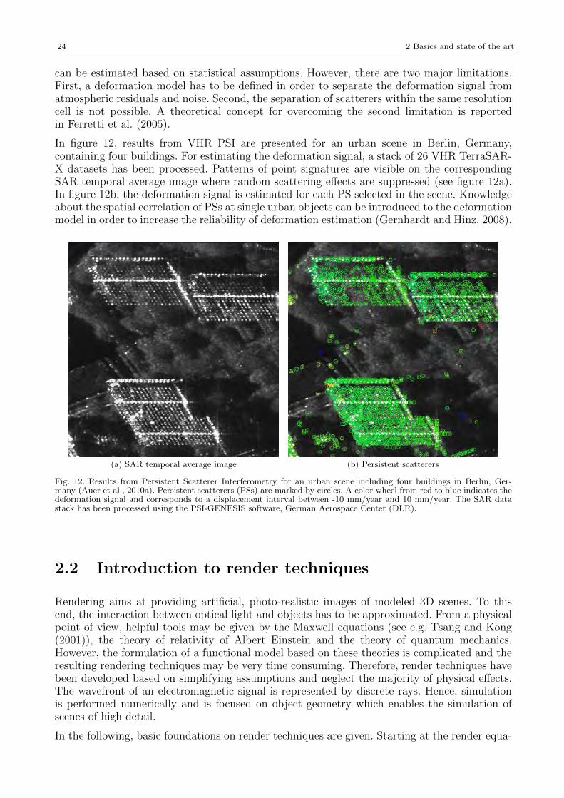
In figure 12, results from VHR PSI are presented for an urban scene in Berlin, Germany,containing four buildings. For estimating the deformation signal, a stack of 26 VHR TerraSAR-X datasets has been processed. Patterns of point signatures are visible on the correspondingSAR temporal average image where random scattering effects are suppressed (see figure 12a).In figure 12b, the deformation signal is estimated for each PS selected in the scene. Knowledgeabout the spatial correlation of PSs at single urban objects can be introduced to the deformationmodel in order to increase the reliability of deformation estimation (Gernhardt and Hinz, 2008).
(a) SAR temporal average image (b) Persistent scatterers
Fig. 12. Results from Persistent Scatterer Interferometry for an urban scene including four buildings in Berlin, Ger-many (Auer et al., 2010a). Persistent scatterers (PSs) are marked by circles. A color wheel from red to blue indicates thedeformation signal and corresponds to a displacement interval between -10 mm/year and 10 mm/year. The SAR datastack has been processed using the PSI-GENESIS software, German Aerospace Center (DLR).
2.2 Introduction to render techniques
Rendering aims at providing artificial, photo-realistic images of modeled 3D scenes. To thisend, the interaction between optical light and objects has to be approximated. From a physicalpoint of view, helpful tools may be given by the Maxwell equations (see e.g. Tsang and Kong(2001)), the theory of relativity of Albert Einstein and the theory of quantum mechanics.However, the formulation of a functional model based on these theories is complicated and theresulting rendering techniques may be very time consuming. Therefore, render techniques havebeen developed based on simplifying assumptions and neglect the majority of physical effects.The wavefront of an electromagnetic signal is represented by discrete rays. Hence, simulationis performed numerically and is focused on object geometry which enables the simulation ofscenes of high detail.
In the following, basic foundations on render techniques are given. Starting at the render equa-
2.2 Introduction to render techniques 25
tion, which theoretically provides an optimum solution, different algorithms for rendering im-ages are briefly introduced. Finally, the relevance of render algorithms for SAR simulation isdiscussed.
2.2.1 The render equation
The major precondition for any functional model approximating global illumination withinan illuminated scene is the conservation of energy. In other words, the sum of the reflected,transmitted and absorbed signal has to be constant at each surface illuminated by a lightsource. In sum, the outgoing radiance from a point ~x, located on a surface, in direction ~$ maybe described as
Io(~x, ~$) = Ie(~x, ~$) + Ir(~x, ~$) + It(~x, ~$) (11)
where
Ie(~x, ~$) is radiance emitted by the surface itself [unit: Wsr·m2 ; sr: steradians],
Ir(~x, ~$) is radiance specular or diffuse reflected at the surface, and It(~x, ~$) is radiance transmitted through the surface.
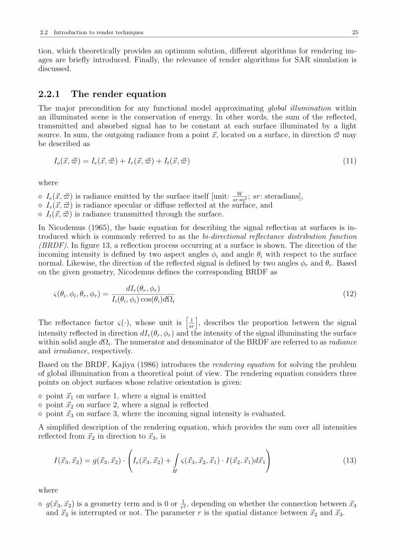
In Nicodemus (1965), the basic equation for describing the signal reflection at surfaces is in-troduced which is commonly referred to as the bi-directional reflectance distribution function(BRDF). In figure 13, a reflection process occurring at a surface is shown. The direction of theincoming intensity is defined by two aspect angles φi and angle θi with respect to the surfacenormal. Likewise, the direction of the reflected signal is defined by two angles φr and θr. Basedon the given geometry, Nicodemus defines the corresponding BRDF as
ς(θi, φi, θr, φr) =dIr(θr, φr)
Ii(θi, φi) cos(θi)dΩi
(12)
The reflectance factor ς(·), whose unit is[
1sr
], describes the proportion between the signal
intensity reflected in direction dIr(θr, φr) and the intensity of the signal illuminating the surfacewithin solid angle dΩi. The numerator and denominator of the BRDF are referred to as radianceand irradiance, respectively.
Based on the BRDF, Kajiya (1986) introduces the rendering equation for solving the problemof global illumination from a theoretical point of view. The rendering equation considers threepoints on object surfaces whose relative orientation is given:
point ~x1 on surface 1, where a signal is emitted point ~x2 on surface 2, where a signal is reflected point ~x3 on surface 3, where the incoming signal intensity is evaluated.
A simplified description of the rendering equation, which provides the sum over all intensitiesreflected from ~x2 in direction to ~x3, is
I(~x3, ~x2) = g(~x3, ~x2) ·
Ie(~x3, ~x2) +∫H
ς(~x3, ~x2, ~x1) · I(~x2, ~x1)d~x1
(13)
where
g(~x3, ~x2) is a geometry term and is 0 or 1r2
, depending on whether the connection between ~x3
and ~x2 is interrupted or not. The parameter r is the spatial distance between ~x2 and ~x3.
26 2 Basics and state of the art
Ie(~x3, ~x2) is the intensity emitted at point ~x2 in direction to point ~x3, i.e. if surface 2 is alight source. ς(~x3, ~x2, ~x1) is the bidirectional reflectance distribution function describing the reflection pro-
cess starting at ~x1, including ~x2, and ending at ~x3. I(~x2, ~x1) is the intensity emitted at point ~x1 in direction to surface ~x2. H is the hemisphere covering the surface marked by point ~x2.
While g(~x3, ~x2), Ie(~x3, ~x2) and ς(~x3, ~x2, ~x1) are assumed to be given by scene geometry andobject materials, I(~x2, ~x1) is unknown. Thus, the main task of render algorithms is to approx-imate the entity of all intensities impinging on point ~x2 at surface 2 from hemisphere H. In itsbasic form, the rendering equation neglects signal diffraction, atmospheric effects, wavelengthdependence, and signal polarization.
Fig. 13. Geometry of bi-directional reflection process (Nicodemus, 1965).
2.2.2 Rendering algorithms
Different algorithms for rendering are reported in the literature which can be considered asapproximations of the rendering equation. The components of a scene to be rendered are iden-tical for all rendering methods: besides the geometry and material of objects, at least one lightsource and a camera is needed. Main differences occur when representating reality, i.e. whenapproximating the render equation. The focus is either on providing photo-realistic images ata high computational cost, e.g. for animated movies, or on providing near-realistic images inreal-time, e.g. for video games. A short history of relevant render algorithms is given in thefollowing.
(Appel, 1968) simulate optical images of objects which are toned by a digital plotter. Usingpoint by point shading, rays are followed in inverse direction starting at the projection center ofthe camera. The main motivation is the simulation of shadow which gives information aboutthe relative position of two or more objects within a simulated scene. Moreover, the visibility ofobjects to the camera can be checked efficiently. However, the detection of intensities is limitedto direct backscattering of type ’diffuse’. Bouknight (1970) present the scanline algorithm wherethe boundaries of 3D objects are transformed into the 2D image plane of the camera. Afterwards,intersections between object boundaries and horizontal scanlines are detected within the image
2.2 Introduction to render techniques 27
plane in order to identify the interior and exterior of projected objects. Eventually, interiorareas visible to the camera are analyzed for intensity contributions. For simplification, theposition of the light source is equal to the camera position. Multiple reflection of signals isneglected. Catmull (1974) adopts the concept of mapping polygons of 3D objects into the 2Dimage plane. However, depth information for checking the visibility of objects, called z-buffer, isprovided and stored for a raster imposed on the image plane, what is called rasterization. Phong(1975) aims at the simulation of curved objects at a sufficient degree and in real-time. Inthis context, reflection models for specular and diffuse reflection are introduced in order toincrease the radiometrical quality of simulated images. Still, multiple reflection of signals is notconsidered. Moreover, the diffuse signal interaction within the scene is not modelled and onlyapproximated by means of a constant value (ambient light).
In Whitted (1980), the ray tracing approach is introduced. While keeping the diffuse reflectionmodel from Phong (1975), the specular reflection model is enhanced in order to include multiplereflections of type ’specular’. Rays are followed in inverse direction starting at the camera. Thediffuse signal interaction between objects is not simulated, i.e. object shadow is represented inblack color or assigned with a intensity constant. Moreover, the sharpness at intensity edges isexaggerated compared to reality. Further information about ray tracing can be found in Glassner(2002). As an enhancement of standard ray tracing, Cook et al. (1984) introduce distributed raytracing. Rays are spatially distributed near the direction of specular reflection for modeling glossand depth of field. Moreover, distributing rays in time enables to simulate motion blur. Heckbertand Hanrahan (1984) aim at solving the discrete sampling problem adherent to ray tracing,which is time-consuming and is affected by aliasing. After transforming 3D object polygons tothe image plane of the camera, beams are used instead of discrete samples in order to detectintensities within the modeled scene (beam tracing). Thereby, intersection polygons are detectedat objects visible to the camera. Specular multiple reflection of signals is approximated by usingthe detected intersection polygons for defining new beams. However, the rendering concept islimited to planar surfaces.
A concept for approximating the transfer of diffuse signals between objects is introducedby Goral et al. (1984) and referred to as Radiosity. Based on a scene representation by meansof flat polygons, the signal impinging on a polygon face is the sum over the diffuse intensitiesscattered from all other polygons. Specular reflections are neglected. Path tracing, a renderingconcept introduced by Kajiya (1986), aims at approximating both specular and diffuse reflec-tions of any kind and, hence, to approximate global illumination. In contrast to the standardray tracing approach, a ray hitting an object is not followed in specular direction. Instead,the direction of the reflected ray is chosen randomly. By emitting a high number of rays foreach image pixel and adding the detected intensities, the render equation is appproximated.However, the computational cost is immense, as a low number of rays per pixel yields noisyimages. Veach and Guibas (1997) propose a new sampling method, called Metropolis sampling,for path tracing. Rays are distributed along initial paths giving a-priori information about theexpected distribution of intensities within the rendered image. Hence, computation time canbe saved due to a reduced number of rays. Jensen (1996) present an alternative approach forthe approximation of global illumination, which is called photon mapping and is reasonable forsimulating caustics.
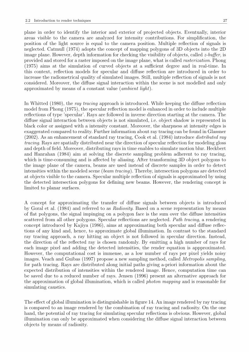
The effect of global illumination is distinguishable in figure 14. An image rendered by ray tracingis compared to an image rendered by the combination of ray tracing and radiosity. On the onehand, the potential of ray tracing for simulating specular reflections is obvious. However, globalillumination can only be approximated when considering the diffuse signal interaction betweenobjects by means of radiosity.
28 2 Basics and state of the art
Fig. 14. Global illumination effect for a multi-body scene. Left: ray tracing neglecting diffuse signal interaction betweenobjects. Ambient light is deactivated. Right: combination of ray tracing and radiosity for the approximation of globalillumination. The model scene is available in the POV-Ray hall of fame (POV-Ray, 2011).
2.2.3 Relevance of render techniques for SAR simulation
As was already indicated above, rendering algorithms are mainly applied for simulations inthe visible spectrum. In optical images, color information depends on the chemical propertyof objects and, hence, differences in backscattering for different signal wavelengths. Moreover,with little exception, the signal wavelength (approx. 380 nm - 750 nm) can be considered asbeing small compared to the roughness of object surfaces. Hence, the simulation of diffusesignal interaction at objects is important while specular effects only have to be added in caseof specific materials, e.g. metallic surfaces or surfaces made of glass. To conclude, standard raytracing is not sufficient for the simulation of optical data since global illumination is requiredfor photo-realistic representation (see example in figure 14).
However, tools given by rendering methods are also applied for simulating signal-object inter-action in case of larger wavelengths. For instance, Ikegami et al. (1991) use ray tracing forcalculating the mean field strength of radio systems along pre-defined profiles within an urbanscene. In Schmitz et al. (2009), beam tracing is applied for simulating the propagation of radiosignals within an urban scene in near real time. In Lehnert (1993), the detection problem ofray tracing is identified when simulating room accoustics. Artificial signal differences occur ifthe size of the detection element is not adapted to the density of rays during ray tracing.
The strength of radar responses from objects is influenced by the roughness and permittivityof surfaces. Signals of constant frequency are emitted and detected. The signal wavelength,e.g. 3.1 cm for X-Band, is comparable to the height deviation of objects or even large, e.g.in case of smooth surfaces at man-made objects. Therefore, specular reflections are expectedto dominate diffuse reflections at urban objects. The importance of diffuse signal interactionbetween objects is of less importance than for simulations in the optical spectrum. However,when using rendering methods for SAR simulation, new reflection models have to be defined orgiven reflection models have to be adapted for describing the interaction of radar signals andobjects.
At present, the application of two rendering methods for SAR simulation is reported in theliterature: rasterization and ray tracing. Rasterization aims at SAR simulation in real-time,e.g.
for simulating direct backscattering of radar signals, e.g. (Rius et al., 1993) (Balz, 2006), for approximating double reflections (Balz and Stilla, 2009), or for checking the visibility of objects (Margarit et al., 2007).
2.3 SAR simulation - state of the art 29
Ray tracing enables the simulation of multiple reflections, e.g. for providing test data for featureextraction algorithms. A detailed literature survey on the simulation of detailed objects basedon ray tracing is given in chapter 2.3.3. The approach presented in this thesis is based on raytracing as well. To this end, the open-source ray tracer POV-Ray is adapted and enhanced inorder to provide output data in SAR geometry. An introduction to POV-Ray and its modelingtools is given in Appendix B.
2.3 SAR simulation - state of the art
2.3.1 Concepts for SAR simulation
In Franceschetti et al. (1995), SAR simulators are cathegorized in image simulators and rawdata simulators. Simulators of the former kind aim at directly simulating SAR images, i.e.without intermediate raw data used as input for a SAR processor. SAR raw data simulatorsare developed in order to provide test data for processing algorithms or for the radiometricanalysis of SAR data.
Early concepts for SAR image simulators concentrate on the simulation of direct backscatteringfrom open areas. Muhleman (1964) presents a reflection model based on ray optics in order toestimate the mean surface slope and the rotation rate of the Venus. Boyell (1969) simulatesdirect backscattering from lunar surfaces in real-time on a television screen. Terrain occlusionsand shadow are detected along ground range profiles. In Holtzman et al. (1978), SAR imagesof rural, homogeneous areas are simulated and are recorded on photographic film in order tosupport information extraction from SAR data. The amount of silver grains on the photographicfilm is calculated based on the radar equation. The spatial correlation of speckle on resolutioncell level is approximated in Raney and Wessels (1988), showing that imposing random specklenoise to a simulated SAR image pixel is not sufficient. Simulation results for airborne SARimages are presented for a rural scene. Gelautz et al. (1998) introduce an approach for simulatingSAR amplitude data for alpine regions. To this end, points of a digital elevation model (DEM)are mapped into the azimuth-range plane and post-processed in order to obtain a regular raster.Eventually, simulated SAR data are used for supporting the projection of real SAR data on aDEM of moderate resolution.
Besides the simulation of rural areas, image simulators are applied for the purpose of provid-ing a-priori knowledge about man-made objects. For instance, ray tracing methods are appliedin Wohlers et al. (1980) for simulating SAR image signatures of airplanes. The main moti-vation is to provide test data for automated object identification. However, the simulation oftargets is limited to direct backscattering. Nasr and Vidal-Madjar (1991) use ray tracing meth-ods for detecting specular reflectors, dihedral, and trihedral geometries, labeled as ’ElementaryGeometric Reflectors (EGRs)’, for each target. Afterwards, the target response is derived bysumming up the signal of EGRs for each resolution cell and is enbedded into SEASAT data.Analyzing the shape of objects in real SAR data is not persued due to the limited resolution ofthe SEASAT satellite. Rius et al. (1993) use rendering tools provided by a graphics workstationfor simulating the radar cross section of 3D objects. Simulation of radiometric information isperformed using physical optics, edge diffraction and signal absorption. Multiple reflections ofradar signals are neglected. Bolter (2001) simulate the direct backscattering of radar signalsfor refining 2.5D building models extracted from multi-aspect airborne InSAR data. Knowl-edge provided by SAR simulation is used for discarding building layover and occluded shadowareas as data source for building reconstruction. Xu and Jin (2006) simulate polarimetric SARdata based on a mapping and projection algorithm in order to provide test data for buildingreconstruction methods. Multiple reflections are accounted for but only simulated within the
30 2 Basics and state of the art
incident field of the radar signal. Rasterization methods are used in Balz (2006) for simulatingSAR images or urban areas in real-time. Depth information of objects visible to the virtualSAR sensor is gathered by a z-buffer. In Balz and Stilla (2009), the approximation of doublereflections of radar signals is included into the simulation approach. Melody (2009) analyze thepath of multiple reflected radar signals for finding the real position of objects. Thus, hintedobjects without direct response but multi-bounce response can be detected within an imagedscene. Brunner (2009) presents a ray tracing approach for simulating the appearance of ba-sic building shapes in VHR SAR data. Simulated SAR data for different incidence angles ofthe radar signal enable to estimate the height of buildings based on correlation methods. Thesimulation of double reflections of radar signals is limited to one azimuth resolution cell.
Simulators for providing SAR raw data are based on physical models describing reflection phe-nomena, e.g. (Tsang and Kong, 2001; Franceschetti et al., 2001). In this context, the geometricaldescription of single objects is simplified or even neglected. Camporeale and Galati (1991) dis-cuss two SAR simulator concepts for the simulation of raw data. End-to-end simulators enablethe analysis of changes to the SAR system response of targets, e.g. the saturation of intensities.In contrast, assuming a constant SAR system response for targets enables to simulate areasof large-scale with reduced calculating time. Franceschetti et al. (1992) define SAR reflectionmodels in order to provide SAR raw data for open terrain. Shadow areas are detected usingray tracing methods. In Franceschetti et al. (2002), the SAR simulation approach is enhancedby reflection models for double and triple bounce at buildings. Simulation results for the ap-proximation of multiple reflections are presented in Franceschetti et al. (2003). Since the focusis on radiometric correctness and on the definition of reflection models in closed form, theSAR simulation approach is limited to basic shapes, e.g. buildings are represented by box mod-els. Bickert et al. (2002) simulate SAR raw data for the purpose of supporting the developmentof a ground moving target indication (GMTI) algorithm. To this end, radar signals of movingtargets are added to a clutter map derived from given SAR data. Speck et al. (2002) presenta raw data simulator based on separate modules for 3D objects, such as buildings or vehicles,and the background. Information about the radar cross section of targets is kept in a data basewhile electromagnetic properties of surfaces are used for approximating backscattering from theground.
Including angular information in cross-range direction, different InSAR simulators are reportedin the literature. For instance, Franceschetti et al. (1998) include signal decorrelation intothe definition of electromagnetic models for the simulation of SAR reflectivity maps. Hence,the disturbance of the interferometric signal is not included artificially to the simulated data.Simulation scenarios for layover situations are not presented. Petit and Adragna (2000) applysimulation techniques for evaluating the loss of coherence in case of direct backscattering ofthe radar signal from sloped surfaces. InSAR simulation methods, using a DEM as input, arepresented by Eineder (2003) in order to enable the prediction of shadow and layover areas formountainous areas of large scale. A grid of points representing the DEM surface is derived byintersecting the DEM with radar signal wavefronts regularly distributed in range. Mori andDe Vita (2004) present a InSAR raw data simulator operating in time domain and consideringthe curvature of the sensor orbit and the earth surface. The approach aims at the simulationof direct backscattering of radar signals for areas of large scale. Focused on urban areas, Thieleet al. (2007a) simulate phase profiles of basic building shapes in case of single bounce of radarsignals and compare it to phase profiled extracted from airborne SAR data. The radiometricalcorrectness of the simulation results is limited since surface backscattering is assumed to onlydepend on the local angle of incidence of the radar signal. In Thiele et al. (2010), the interferenceof the signal phase is simulated for adjacent buildings represented by boxes whose heights vary.
2.3 SAR simulation - state of the art 31
2.3.2 VHR SAR simulation for urban areas
The strength of radar signals backscattered to the SAR sensor depends on surface parameters(roughness, correlation length, permittivity) but also on the geometry of objects, which maybe characterized by regular shapes such as dihedrals or trihedrals. In SAR data of low ormedium resolution, most objects are smaller than the resolution of the SAR system. Hence,with regard to SAR simulation, an object representation by means of backscatter coefficientsmay be appropriate, as shown e.g. by Holtzman et al. (1978) or Speck et al. (2002). Whenusing this method, acceptable results are expected for homogeneous areas of large scale. Incontrast, SAR simulation approaches for supporting the interpretation of VHR SAR data haveto consider the geometry of a scene of interest as the signal response of single objects may bedistributed over a high number of pixels.
In case of multiple reflections of radar signals at single objects, the description of object geom-etry is expected to be fundamental. A compromize has to be found between the radiometricand geometric correctness of simulation results. A reliable representation of the radiometry ofmultiple reflections is enabled by equations in closed form based on the Maxwell equations. Forinstance, both the position and the signal power of double bounce signatures corresponding tosignal interaction with building walls and the surrounding ground can be simulated. Moreover,the inversion of reflection models in closed form enables the extraction of object heights basedon the intensity of SAR image signatures (Franceschetti et al., 2007). For this purpose, sur-face parameters of objects have to be known a-priori, what may be challenging for man-madeobjects Brunner et al. (2009). Moreover, the simulation of objects has to rely on basic objectshapes, e.g. box models (Franceschetti et al., 2002).
However, non-metallic building corners having a sidelength of 10 cm are anticipated to be vis-ible in VHR SAR data, even if their extent is much smaller than the size of a resolution cell.Examples for building parts forming small corners may be windows, balconies, facade protru-sions or roof structures. Hence, a high level of detail of building models may be required inorder to enable the simulation of SAR image signatures corresponding to multiple reflections ofthe radar signal. Rendering methods such as rasterization or ray tracing have been developedfor simulating object models of that detailedness at the cost of limited radiometric correctnessof rendered images. The propagation of signal wave fronts is approximated by discrete samples– rays – which are not appropriate for substituting radar reflection models in closed form. How-ever, since the work presented in this thesis aims at the geometrical analysis of salient signaturesin VHR SAR data, the focus has to be put on the geometrical correctness of simulation results.Ray tracing methods are applied for sampling modeled scenes containing man-made objects andfor providing output data in SAR geometry. Due to the duality of geometry and radiometryin case of multiple reflections of radar signals, limitations with regard to the correctness of thesimulated signal strength have to be accepted.
2.3.3 Discussion of most related work
At this point, work related to the simulation approach presented in this thesis is introduced.Three relevant simulators – SPECRAY-EM/FERMAT, GRECOSAR, and PIRDIS – are dis-cussed as they show similarities to the simulation approach presented in this thesis:
ray tracing methods are applied for simulating radar signals, multiple reflections of radar signals are accounted for, simulation of VHR SAR data is enabled and persued, and detailed object models may be simulated.
SPECRAY-EM/FERMAT has been developed in a joint project of ONERA (Office Nationald’Etudes et de Recherches Aerospatiales) and OKTAL-SE, France, combining knowledge aboutelectromagnetics, render techniques and the handling of data bases. The main objectives are the
32 2 Basics and state of the art
calculation of the radar cross section of objects, the prediction of sensor capabilities, and thesimulation of objects within environments for testing target detection algorithms. In advance tothe simulation procedure, modeled object scenes have to be represented by means of triangles.Sampling of scenes is performed by means of tubes defined by a perspective view in line-of-sight of the sensor (Mametsa et al., 2001). The synthetic aperture is simulated and azimuthprocessing effects are accounted for. Simulation results are reported for single objects (Hammeret al., 2008) and open terrain including objects (Latger et al., 2005). Models for the reflection ofradar signals are defined for metallic, diffuse and specular surfaces. The strength of the signalresponse is approximated using high-frequency RCS prediction techniques (Knott et al., 2004),namely geometrical optics (GO) for specular reflection and physical optics (PO) for diffusereflection. Speckle, atmospheric effects, and signal diffraction may be simulated (Berges et al.,2004). Multiple reflections of radar signals are considered. Simulation results are provided inthe azimuth-range or azimut-ground-range plane. A cross-comparison to other SAR simulatorsbased on render techniques can be found in Hammer et al. (2008).
GRECOSAR aims at the simulation of polarimetric SAR data of single objects. The devel-opment of the simulator is based on the assumption that object classification is improved byincluding polarimetric information. Thus, polarimetric SAR data are simulated for testing clas-sification algorithms. Simulation results are presented for vessel models (Margarit et al., 2006)and building models of high detail (Margarit et al., 2007). The approach is based on GRECO(Graphical Electromagnetic Computing), a tool for simulating the radar cross section of ob-jects on a graphics workstation (Rius et al., 1993). Margarit et al. (2006) adapt GRECO tothe imaging geometry of a SAR and combine it with a processor for SAR raw data. Curvedobjects are approximated by triangles in order to enable a intersection test for rays emitted bythe virtual SAR antenna. The backscattering from perfectly conducting surfaces is evaluatedusing physical optics (PO) while multiple reflections are approximated by a combination ofgeometrical and physical optics (GO + PO). After simulation of the synthetic aperture, theSAR raw data are post-processed. Scattering maps are created by polarimetric decompositionof the simulated SAR data and image features are identified, e.g. the distribution of dihedralsand trihedrals characterizing vessels for different aspect angles (Margarit et al., 2009).
PIRDIS (Platform-Independent Range/Doppler Image Simulation) is a simulator for SAR am-plitude data introduced by Meyer-Hilberg (2006). The main objective of the simulation ap-proach is to provide test data for SAR ground moving target indication (GMTI). Moreover,data can be simulated for certain SAR imaging geometries in order to evaluate the performanceof future SAR systems. Multiple reflection and polarization of the radar signal is consideredas well as atmospheric effects. Physical optics (PO) is used for simulating the backscatteringfrom terrain. Eventually, the simulated SAR image is composed by signal response from thebackground and signal response from moving or non-moving objects (Meyer-Hilberg et al.,2008).
As mentioned above, all related simulation approaches are focused on object geometry and,hence, consider multiple reflections at objects. The main motivation of the simulation ap-proaches is to provide a reliable approximation of real SAR data in the azimuth-range planegiven a certain amount of a-priori knowledge about the scene to be simulated, e.g. object ge-ometry, object movements, surface characteristics or disturbing factors such as certain weatherconditions or noise. To this end, radar reflection models are integrated in the ray tracing en-vironment and SAR image characteristics like speckle or the sinc-function as the response ofpoint scatterers are considered. With regard to the application of simulated data, simulationsare conducted for different purposes:
(1) Tools for information extraction from SAR data can be tested, for instance, algorithms forobject detection (major objective of SPECRAY-EM/FERMAT and PIRDIS) or for objectclassification (GRECOSAR).
(2) Simulated SAR data can be visually compared to SAR data in order to interpret imaged
2.3 SAR simulation - state of the art 33
scenes (major objective of SPECRAY-EM/FERMAT).(3) Future SAR system performances can be tested (major objective of SPECRAY-
EM/FERMAT and PIRDIS).
In any case, the ideal simulation result would be a copy of real SAR data minimizing systematicerrors in provided test data. The interpretation of SAR image signatures is performed on theimage level, i.e. the expression ’scatterer’ is linked to a salient image pixel. Investigating theorigin of SAR image signatures on the object level is not enabled.
However, the interpretation of salient SAR image features corresponding to multiple reflectionsof the radar signal requires additional support beyond the simulation of data in the azimuth-range plane. The expression ’scatterer’ has to be linked to the geometry of structures withinsimulated scenes. For this purpose, methods are required for analyzing the correspondance ofdominant SAR image signatures to regular and non-regular object geometries. More specifically,the inversion of the SAR imaging process has to be simulated. Still, the nature of dominantsignatures on SAR images is not known in detail what is crucial when evaluating the reliabilityand meaning of SAR products, e.g. deformation signals for single objects detected by PSI.As introduced in Section 2.3.1, ray tracing methods are applied in Nasr and Vidal-Madjar(1991) for seeking dihedrals, trihedrals, and specular backscattering surfaces characterizingthe signal response of objects. To this end, a-priori knowledge about the geometrical shapeof structures provoking dominant SAR image signatures is introduced. However, salient SARimage signatures may also occur at non-ideal scatterers such as trihedrals without tips, non-orthogonal corners, or corners partly occluded with respect to the line-of-sight of the SARsensor.
For all related SAR simulation approaches, SAR products are interpreted in 2D image space.SPECRAY-EM/FERMAT and PIRDIS simulate the distribution of signals in azimuth andrange. Accordingly, scatterers within the same resolution cell are not spatially separated duringthe simulation process. Layover situations can not be resolved, for instance, in order to find thenumber of dominant scatterers corresponding to a SAR image pixel. Besides map in the azimuth-range plane, GRECOSAR enables to include the third dimension by simulating interferometricSAR data. However, the spatial distribution of signals in height is visualized on 2D imagesindicating the SAR sensor’s line-of-sight.
The SAR simulation approach presented in this thesis has been developed in order to meet thelimitations discussed above. New methods have to be developed for investigating the nature ofdominant scatterers in urban areas based on simulated SAR data. To this end, the 3D positionof phase centers, i.e. including the elevation domain, is directly simulated. Basic ideas and casestudies with regard to the SAR simulation concept are presented in Auer et al. (2008), Aueret al. (2009b), Auer et al. (2009a), Auer et al. (2010b), and Auer et al. (2010a). A detailedintroduction and discussion of the developed SAR simulation methods is given in chapters 5and 6.
34 3 Introduction to RaySAR
3 Introduction to RaySAR
3.1 3D SAR simulation approach - new aspects
The SAR simulation approach presented in this thesis is focused on developing new methodsfor supporting the interpretation of salient signatures on VHR SAR images corresponding toman-made objects. In this regard, the SAR simulator, named RaySAR, aims at solving thelimitations of related simulators discussed in Chapter 2.3.3 where the interpretation of signaldistributions is conducted on 2D image planes. In sum, the simulation approach addresses threenew aspects:
(1) 3D SAR simulation in azimuth, range, and elevation.(2) Methods for the geometrical analysis of scatterers are provided.(3) The inversion of the SAR imaging system is simulated.
to (1)
A new 3D SAR simulator based on ray tracing methods, named RaySAR, is proposed enablingthe analysis of signatures in azimuth, range, and elevation. To this end, the open-source raytracer POV-Ray (Persistence of Vision Ray Tracer) is adapted and enhanced for providing out-put data in SAR imaging geometry. The SAR system is represented by a camera characterizedby orthographic projection in azimuth and elevation as well as by a signal source emitting par-allel light. Simulation applications are focused on the simulation of urban environments withlimited extent. Focusing of multiple reflections is performed directly without data gatheringalong a virtual synthetic aperture. RaySAR simulates an ideal SAR system having infinite res-olution in azimuth, range, and elevation, i.e. a corner reflector is focused to a point in 3D space.Hence, several scatterers contributing signals to the same SAR image pixel can be separatedin elevation. It is not the purpose of RaySAR to simulate the entire imaging chain consideringthe pulse repetition frequency (PRF) of the SAR system and speckle. In contrast, emphasizingSAR image signatures may be welcome for understanding the geometrical shape of objects inSAR data.
to (2)
Simulated SAR data only form a basis product where SAR image signatures of interest areselected for further analysis. Different reflection levels can be assigned to separate image layersin order to focus on a bounce level of interest, e.g. double or triple bounce. Image pixels con-taining specular reflections can be distinguished from pixels only characterized by diffuse signalresponse. The elevation of scatterers can be displayed along profiles pointing in azimuth andrange. Moreover, the distribution of intensities in elevation can be simulated for selected pixels,which enables to find the number of scatterer responses integrated into the same resolutioncell. Finally, phase centers simulated in SAR imaging geometry can be mapped into detailed3D object models for analyzing the physical correspondance to object features.
to (3)
RaySAR includes methods for identifying object surfaces contributing to salient image signa-tures. Hence, object surfaces hit by the virtual radar signal are geometrically linked to signa-tures within the simulated image, i.e. the SAR imaging system can be inverted. Starting in thereal SAR image, signatures can be cross-compared to signatures in the simulated SAR image.Afterwards, surfaces contributing to the signature can be identified within the simulated 3Dobject model. Thereby, the discussion of the nature of scatterers is shifted from signatures in
3.2 Motivation for using POV-Ray 35
the SAR image plane, e.g. points or lines, to the geometry of structures in the object space,e.g. dihedrals, trihedrals or non-regular reflectors.
3.2 Motivation for using POV-Ray
In order to meet the requirements summarized at the end of Chapter 1.2, the decision was madeto use render methods for SAR simulation. In this context, the minor objective ’integrationand enhancement of available software’ (Chapter 1.2) was chosen by purpose. When using andadapting tools of available software, the focus can be set on the the main component of thiswork: the analysis of the nature of scatterers which is mainly covered by research beyond thesimulation of SAR data in the azimuth-range plane. Finally, the open-source ray tracer POV-Ray was chosen as appropriate platform for developing a SAR simulator. An brief introductionto POV-Ray can be found in Chapter B.1. In summary, the ray tracing package fitted well intothe defined requirement profile due to the following properties:
POV-Ray comprises a variety of fast simulation tools. The POV-Ray source code has been continously developed and improved by a huge commu-
nity since 1991. Basic modules are thoroughly tested and free from programming errors. The inclusion of own developments is possible due to free access to its source code. POV-Ray uses an efficient concept for tracing rays, more specifically, ray tracing in reverse
direction, which starts at the center of each image pixel and follows rays backward on theirway to the signal source. POV-Ray offers appropriate interfaces for importing object models of high detail. Moreover,
the representation of the radar signal by means of rays enables the simulation of analyticalshapes such as curves or spheres.
Basic shapes and the imaging geometry of the SAR sensor within a virtual scene can be definedin the POV-Ray editor. Moreover, basic algorithms such as the ray tracing procedure, inter-section tests between rays and objects or the detection of intensities or shadows can be usedas provided by the basic POV-Ray software. However, own developments have been added toPOV-Ray’s source code in order to provide output data in SAR geometry.
3.3 SAR simulation concept - modeling, sampling, 3D
analysis
An overview of the SAR simulation concept is given in figure 15. Basically, the processingchain contains three main components: modeling, sampling by the ray tracer and scattereranalysis. Modeling has to be performed in order to provide necessary input information aboutobjects to be simulated. To this end, the geometry of objects has to be described, e.g. by meansof analytical shapes or polygons (see Chapter 4.1 for detailed information). Moreover, surfacecharacteristics have to be assigned to all objects for steering the reflection behavior (see Chapter4.3). Finally, the position and parameters of the virtual SAR have to be added to the modeledscene (see Chapter 4.2). After the definition of rendering settings, sampling of the object sceneis conducted based on ray tracing methods provided by POV-Ray (see Chapter 5). For eachsignal detected in the scene the following information is derived:
the 3D-position and signal amplitude corresponding to detected signal contributions, bounce level information for each detected signal, flags for marking specular directions, and
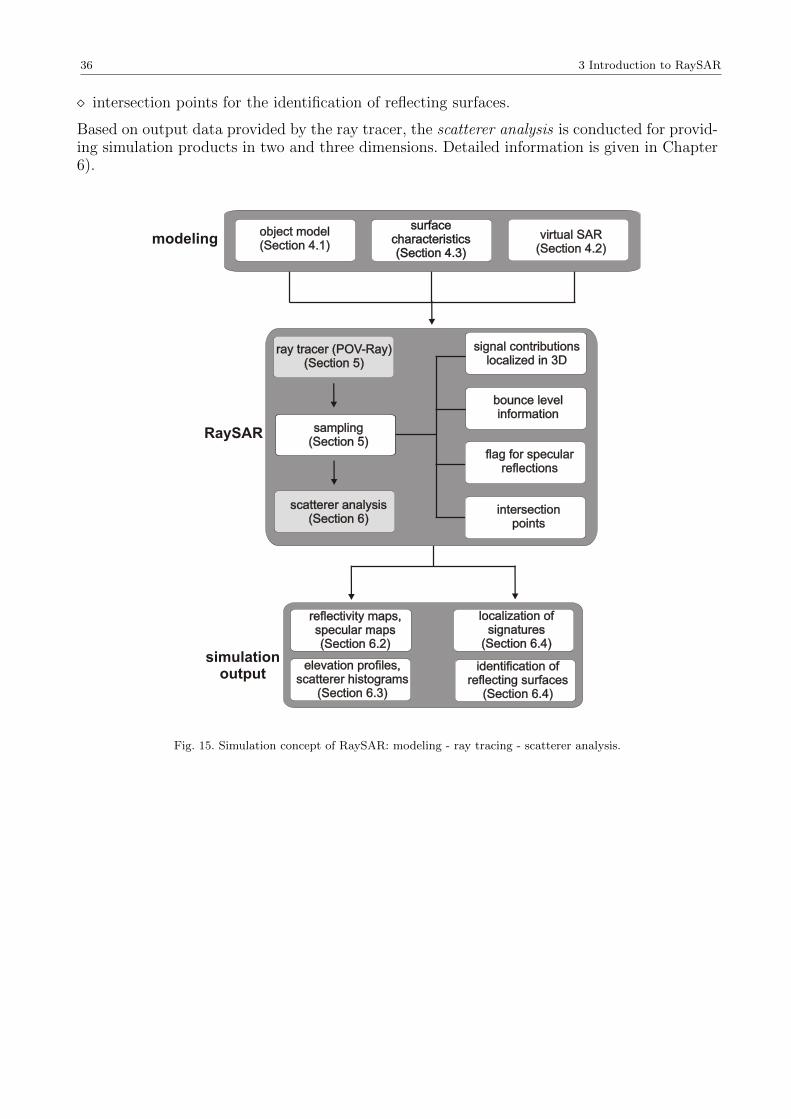
36 3 Introduction to RaySAR
intersection points for the identification of reflecting surfaces.
Based on output data provided by the ray tracer, the scatterer analysis is conducted for provid-ing simulation products in two and three dimensions. Detailed information is given in Chapter6).
Fig. 15. Simulation concept of RaySAR: modeling - ray tracing - scatterer analysis.
4 Modeling - definition of 3D scenes 37
4 Modeling - definition of 3D scenes
In advance to the ray tracing procedure, the object scene to be simulated has to be defined.To this end, the geometry of objects has to be represented by means of 2.5D or 3D models.Backscattering characteristics have to be assigned to all object surfaces for modeling the re-flection of radar signals. Finally, the imaging geometry of the SAR system has to be defined inthe coordinate system of the object scene. Details with respect to the different modeling stepsare given in this chapter.
4.1 Data sources for 3D building models
Geometrical information about buildings can be provided on several ways, e.g. by own modelingor by importing available building models into the simulation environment. A brief introductionand discussion of different sources for building models is given in the following.
Modeling in POV-Ray editor
Modeling in the POV-Ray editor is reasonable for the simulation of basic shapes such as cubes,curved surfaces, or corners. Constructive solid geometry (CSG) may be appropriate in order tocreate objects characterized by specific geometrical shapes (Hoffmann, 1989). As main advan-tage of direct modeling in POV-Ray, simultaneous access to object coordinates, transformationparameters, camera parameters and render settings is provided. Hence, case studies for basicshapes can be conducted in a reasonable amount of time. In contrast, the major disadvantageis that modeling is performed in a text editor where objects are not visually displayed. Ac-cordingly, the correctness of the object geometry can not be controlled in a CAD-environmentand has to be checked by rendering images. Moreover, the time needed for modeling increasessignificantly when increasing the level of detail of objects.
From practical experience, the modeling capability of the POV-Ray text editor was helpfulfor controlling the correctness of the SAR simulation approach, e.g. the radar signal responsecorresponding to a corner reflector represented by three polygons. Moreover, fine tuning of theSAR imaging geometry and editing of surface parameters has to be conducted in the POV-Rayeditor (see chapter B.2).
Modeling in CAD software
Compared to modeling in the POV-Ray editor, CAD software offers instant display of objectsfor visual controlling. Specific modeling tools for directly providing POV-Ray render files areavailable, e.g. Moray (Moray, 2011) or Wings3D (Wings3D, 2011). Generally, any object modelto be simulated by RaySAR has to be integrated in the POV-Ray environment. Thus, objectmodels created by using CAD software such as 3ds Max, Maya, or AutoCAD have to betransformed in the POV-Ray format.
With regard to the simulation approach, the creation of own building models of high detailby using CAD-software was not conducted. Basic shapes were modeled in the POV-Ray editorwhile buildings models of high detail were provided by partners. Even if the modeling of objectsin CAD-software is much faster than in the POV-Ray editor, it is still very time consuming.Furthermore, detailed information about the geometry of objects has to be given a-priori, e.g.by architectural plans.
38 4 Modeling - definition of 3D scenes
Import of 3D models with free access
Building models of many popular buildings are available on the internet, either on homepagescorresponding to building sights, e.g. the Eiffel tower (Eiffel, 2011) or on building data bases,e.g. GoogleTM 3D Warehouse (Google, 2011). When using these models as input for the SARsimulator, the modeling effort is reduced to the definition of the SAR imaging geometry andthe adaptation of surface reflection characteristics in the POV-Ray editor.
However, significant drawbacks have to be mentioned at this point. The majority of down-loadable 3D building models lack in reliability measures as no information is given about thecreation of models and the accuracy of data sources. In most of the cases, building detailsare roughly approximated by a basic geometrical description, e.g. facades represented by flatpolygons, imposed with 2D textures suggesting the 3D geometry of building features. Hence,from the radar point of view, the level of detail of most building models is low. Moreover, theaccess to specific model components is often limited and constant backscattering characteristicshave to be selected for all surfaces. The transformation of common CAD model formats into thePOV-Ray format may introduce changes to the model scene which can be avoided when directlymodeling in the POV-Ray editor. Finally, the application of SAR simulation methods becomesopportunistic since the selection of test sites is driven by the availability and accessibility of3D models.
To conclude, the application of free accessable 3D models with unknown correctness for SARsimulation is only reasonable for case studies. In this context, basic reflection phenomena can beinvestigated at objects having a moderate level of detail. In any case, reliable SAR simulationsuch as the analysis of reflection phenomena for selected SAR image pixels is not enabled.
City models
The creation of city models is mostly initiated by city governments. Hence, these models are ofspecial interest for SAR simulation since the reliability of data used for providing the buildingmodels is known. The level of detail ranges from 2.5D models characterized by flat walls to3D models including facades details. Models of the latter case may especially serve simulationmethods focused on the inversion of the SAR imaging process. Besides, the accessability tomodel features may be enabled due to the given contact to the model provider, e.g. for assigningspecific backscattering characteristics to different building parts. Hence, systematic radiometricerrors can be reduced in combination with a high geometrical correctness of simulation results.While city models of moderate level of detail are developed for areas of large scale, buildingmodels of high detail are only available for selected and popular buildings. In this thesis, theanalysis of reflection phenomena for selected SAR image pixels is based on detailed buildingmodels taken from city models.
Creating models based on measured data
The data basis for the creation of building models can be provided by airborne and terrestriallaserscanning (LiDAR) or photogrammetry. Point clouds of high density are required for rep-resenting edges or curved surfaces characterizing building features. From practical experience,the extraction of facade information from data captured by airborne sensors is challenging dueto data gaps, e.g. due to occlusion by vegetation or undersampling of small building featuressuch as window structures or balconies. For testing the RaySAR simulation approach, buildingmodels have been created based on multi-aspect airborne LiDAR data captured by the RIEGLLMS-Q560 airborne laserscanner. While the creation of 2.5D building models was enabled with-out any complications, the full representation of facade details relevant for SAR simulation wasimpossible. In further studies, the fusion of airborne and terrestrial laserscanning data may bereasonable for solving this problem.
4.2 Design of the virtual SAR system 39
4.2 Design of the virtual SAR system
A real SAR system employs central perspective in elevation in combination with orthogonalscanning in azimuth. For spatially limited areas, e.g. individual buildings, and spaceborne geom-etry, the central perspective in elevation can be well approximated by orthographic projection.In other words, for a local scene located in the far field with respect to the SAR sensor, thewavefront can be assumed to be flat.
Using an orthographic projection offers several advantages: first, a 2-D orthographic cameratype is readily available in POV-Ray. Second, the simulation results become independent of thespatial distance between the virtual SAR and the simulated object. Hence, zooming into theobject to be simulated is enabled. Finally, an ideal SAR system can be simulated for detectingthe positions of signal responses in azimuth, range, and elevation (see chapter 5.1). As maindisadvantage, the simulation approach is bound to local scenes where the angle of incidenceis assumed to be constant. Mapping errors in range depend on the difference between theassumed incidence angle and the true incidence angle and will increase when the simulatedarea is enlarged. For reducing the problem, urban areas of large scale may be split up into tileswhose simulated data are connected afterwards. In any case, mapping errors will occur and willbe maximum at the seam lines between adjacent tiles.
Figure 16 summarizes the design of the virtal SAR system by means of a basic example wherethe object scene to be simulated is represented by two spheres. Instead of modeling the syntheticaperture by moving a virtual SAR, a static system is used for directly simulating SAR data.The imaging geometry and extent of the simulated area is defined using the parameters of theorthographic camera (see Appendix B.2). In case of a monostatic system, both the orthographiccamera and the signal source are located at the same position in space. The POV-Ray sensorcoordinate system and the coordinate system of the virtual SAR are linked as follows:
the azimuth axis corresponds to the horizontal axis of the sensor plane. the elevation axis corresponds to the vertical axis of the sensor plane. the range axis is oriented perpendicularly to the sensor plane. Along this axis, depth infor-
mation is provided by tracing rays.
The local incidence angle and the aspect angle with repect to the imaged object have to beknown for adapting the SAR imaging geometry. The detection of shadow along all scan positionsin azimuth is enabled by including a cylindrical light source emitting parallel light (see AppendixB.2). Constant signal illumination is guaranteed for all objects within the light cylinder.
4.3 SAR simulation radiometry
4.3.1 Reflection models for SAR simulation
The RaySAR models for the reflection of radar signals are based on reflection models given byPOV-Ray (see Appendix B.2). To this end, the parameters of the POV-Ray models are adaptedto approximate the reflection of radar signals. First, the radar signal emitted at a SAR system isrepresented by a vector containing normalized intensity values, i.e. color rgb < 1, 1, 1 >. SinceSAR systems emit a single frequency signal, e.g. in X-Band, only one POV-Ray ’color’ channelis required for SAR simulation. Instead of simulating continous wavefronts, the radar signal isapproximated by means of rays. The effect of surface colors on reflected signals is disabled bynormalization, i.e. color rgb < 1, 1, 1 >. Moreover, textures of 3D object models are removed.Hence, signals detected by the ray tracer only depend on
the imaging geometry with respect to the simulated object
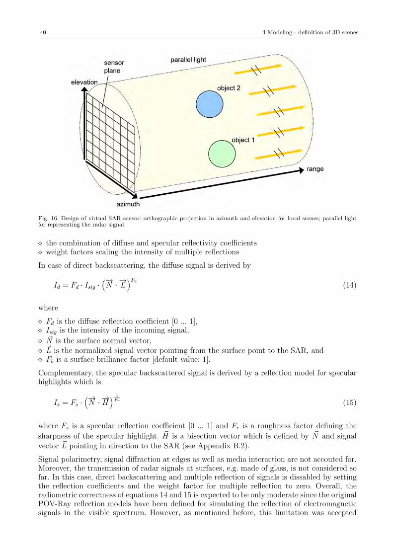
40 4 Modeling - definition of 3D scenes
Fig. 16. Design of virtual SAR sensor: orthographic projection in azimuth and elevation for local scenes; parallel lightfor representing the radar signal.
the combination of diffuse and specular reflectivity coefficients weight factors scaling the intensity of multiple reflections
In case of direct backscattering, the diffuse signal is derived by
Id = Fd · Isig ·(−→N · −→L
)Fb(14)
where
Fd is the diffuse reflection coefficient [0 ... 1], Isig is the intensity of the incoming signal,
~N is the surface normal vector, ~L is the normalized signal vector pointing from the surface point to the SAR, and Fb is a surface brilliance factor [default value: 1].
Complementary, the specular backscattered signal is derived by a reflection model for specularhighlights which is
Is = Fs ·(−→N · −→H
) 1Fr (15)
where Fs is a specular reflection coefficient [0 ... 1] and Fr is a roughness factor defining the
sharpness of the specular highlight. ~H is a bisection vector which is defined by ~N and signalvector ~L pointing in direction to the SAR (see Appendix B.2).
Signal polarimetry, signal diffraction at edges as well as media interaction are not accouted for.Moreover, the transmission of radar signals at surfaces, e.g. made of glass, is not considered sofar. In this case, direct backscattering and multiple reflection of signals is dissabled by settingthe reflection coefficients and the weight factor for multiple reflection to zero. Overall, theradiometric correctness of equations 14 and 15 is expected to be only moderate since the originalPOV-Ray reflection models have been defined for simulating the reflection of electromagneticsignals in the visible spectrum. However, as mentioned before, this limitation was accepted
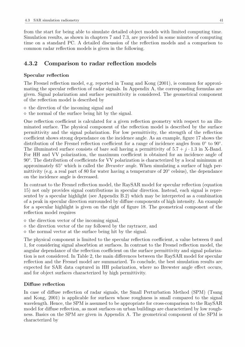
4.3 SAR simulation radiometry 41
from the start for being able to simulate detailed object models with limited computing time.Simulation results, as shown in chapters 7 and 7.3, are provided in some minutes of computingtime on a standard PC. A detailed discussion of the reflection models and a comparison tocommon radar reflection models is given in the following.
4.3.2 Comparison to radar reflection models
Specular reflection
The Fresnel reflection model, e.g. reported in Tsang and Kong (2001), is common for approxi-mating the specular reflection of radar signals. In Appendix A, the corresponding formulas aregiven. Signal polarization and surface permittivity is considered. The geometrical componentof the reflection model is described by
the direction of the incoming signal and the normal of the surface being hit by the signal.
One reflection coefficient is calculated for a given reflection geometry with respect to an illu-minated surface. The physical component of the reflection model is described by the surfacepermittivity and the signal polarization. For low permittivity, the strength of the reflectioncoefficient shows strong dependance on the incidence angle. As an example, figure 17 shows thedistribution of the Fresnel reflection coefficient for a range of incidence angles from 0 to 90.The illuminated surface consists of bare soil having a permittivity of 5.7 + j · 1.3 in X-Band.For HH and VV polarization, the maximum coefficient is obtained for an incidence angle of90. The distribution of coefficients for VV polarization is characterized by a local minimum atapproximately 65 which is called the Brewster angle. When simulating a surface of high per-mittivity (e.g. a real part of 80 for water having a temperature of 20 celsius), the dependanceon the incidence angle is decreased.
In contrast to the Fresnel reflection model, the RaySAR model for specular reflection (equation15) not only provides signal contributions in specular direction. Instead, each signal is repre-sented by a specular highlight (see Appendix B.2) which may be interpreted as a combinationof a peak in specular direction surrounded by diffuse components of high intensity. An examplefor a specular highlight is given on the right of figure 18. The geometrical component of thereflection model requires
the direction vector of the incoming signal, the direction vector of the ray followed by the raytracer, and the normal vector at the surface being hit by the signal.
The physical component is limited to the specular reflection coefficient, a value between 0 and1, for considering signal absorbtion at surfaces. In contrast to the Fresnel reflection model, theangular dependance of the reflection coefficient on the surface permittivity and signal polariza-tion is not considered. In Table 2, the main differences between the RaySAR model for specularreflection and the Fresnel model are summarized. To conclude, the best simulation results areexpected for SAR data captured in HH polarization, where no Brewster angle effect occurs,and for object surfaces characterized by high permittivity.
Diffuse reflection
In case of diffuse reflection of radar signals, the Small Perturbation Method (SPM) (Tsangand Kong, 2001) is applicable for surfaces whose roughness is small compared to the signalwavelength. Hence, the SPM is assumed to be appropriate for cross-comparison to the RaySARmodel for diffuse reflection, as most surfaces on urban buildings are characterized by low rough-ness. Basics on the SPM are given in Appendix A. The geometrical component of the SPM ischaracterized by
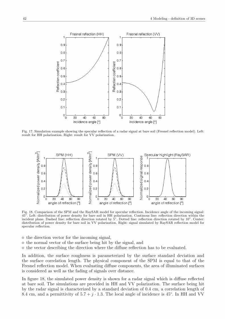
42 4 Modeling - definition of 3D scenes
Fig. 17. Simulation example showing the specular reflection of a radar signal at bare soil (Fresnel reflection model). Left:result for HH polarization. Right: result for VV polarization.
Fig. 18. Comparison of the SPM and the RaySAR model for specular reflection. Incidence angle of the incoming signal:45. Left: distribution of power density for bare soil in HH polarization. Continous line: reflection direction within theincident plane. Dashed line: reflection direction rotated by 5. Dotted line: reflection direction rotated by 10. Center:distribution of power density for bare soil in VV polarization. Right: signal simulated by RaySAR reflection model forspecular reflection.
the direction vector for the incoming signal, the normal vector of the surface being hit by the signal, and the vector describing the direction where the diffuse reflection has to be evaluated.
In addition, the surface roughness is parameterized by the surface standard deviation andthe surface correlation length. The physical component of the SPM is equal to that of theFresnel reflection model. When evaluating diffuse components, the area of illuminated surfacesis considered as well as the fading of signals over distance.
In figure 18, the simulated power density is shown for a radar signal which is diffuse reflectedat bare soil. The simulations are provided in HH and VV polarization. The surface being hitby the radar signal is characterized by a standard deviation of 0.4 cm, a correlation length of8.4 cm, and a permittivity of 5.7 + j · 1.3. The local angle of incidence is 45. In HH and VV
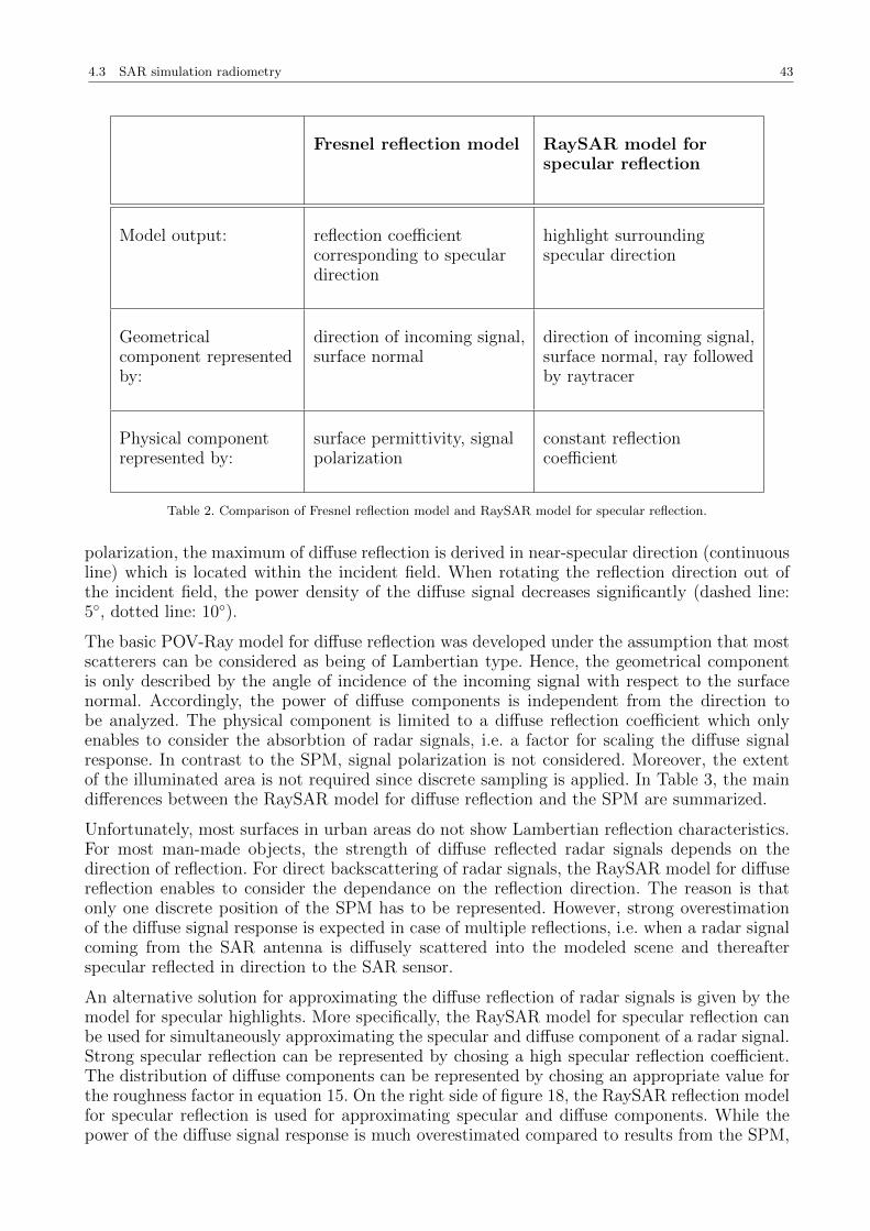
4.3 SAR simulation radiometry 43
Fresnel reflection model RaySAR model forspecular reflection
Model output: reflection coefficientcorresponding to speculardirection
highlight surroundingspecular direction
Geometricalcomponent representedby:
direction of incoming signal,surface normal
direction of incoming signal,surface normal, ray followedby raytracer
Physical componentrepresented by:
surface permittivity, signalpolarization
constant reflectioncoefficient
Table 2. Comparison of Fresnel reflection model and RaySAR model for specular reflection.
polarization, the maximum of diffuse reflection is derived in near-specular direction (continuousline) which is located within the incident field. When rotating the reflection direction out ofthe incident field, the power density of the diffuse signal decreases significantly (dashed line:5, dotted line: 10).
The basic POV-Ray model for diffuse reflection was developed under the assumption that mostscatterers can be considered as being of Lambertian type. Hence, the geometrical componentis only described by the angle of incidence of the incoming signal with respect to the surfacenormal. Accordingly, the power of diffuse components is independent from the direction tobe analyzed. The physical component is limited to a diffuse reflection coefficient which onlyenables to consider the absorbtion of radar signals, i.e. a factor for scaling the diffuse signalresponse. In contrast to the SPM, signal polarization is not considered. Moreover, the extentof the illuminated area is not required since discrete sampling is applied. In Table 3, the maindifferences between the RaySAR model for diffuse reflection and the SPM are summarized.
Unfortunately, most surfaces in urban areas do not show Lambertian reflection characteristics.For most man-made objects, the strength of diffuse reflected radar signals depends on thedirection of reflection. For direct backscattering of radar signals, the RaySAR model for diffusereflection enables to consider the dependance on the reflection direction. The reason is thatonly one discrete position of the SPM has to be represented. However, strong overestimationof the diffuse signal response is expected in case of multiple reflections, i.e. when a radar signalcoming from the SAR antenna is diffusely scattered into the modeled scene and thereafterspecular reflected in direction to the SAR sensor.
An alternative solution for approximating the diffuse reflection of radar signals is given by themodel for specular highlights. More specifically, the RaySAR model for specular reflection canbe used for simultaneously approximating the specular and diffuse component of a radar signal.Strong specular reflection can be represented by chosing a high specular reflection coefficient.The distribution of diffuse components can be represented by chosing an appropriate value forthe roughness factor in equation 15. On the right side of figure 18, the RaySAR reflection modelfor specular reflection is used for approximating specular and diffuse components. While thepower of the diffuse signal response is much overestimated compared to results from the SPM,
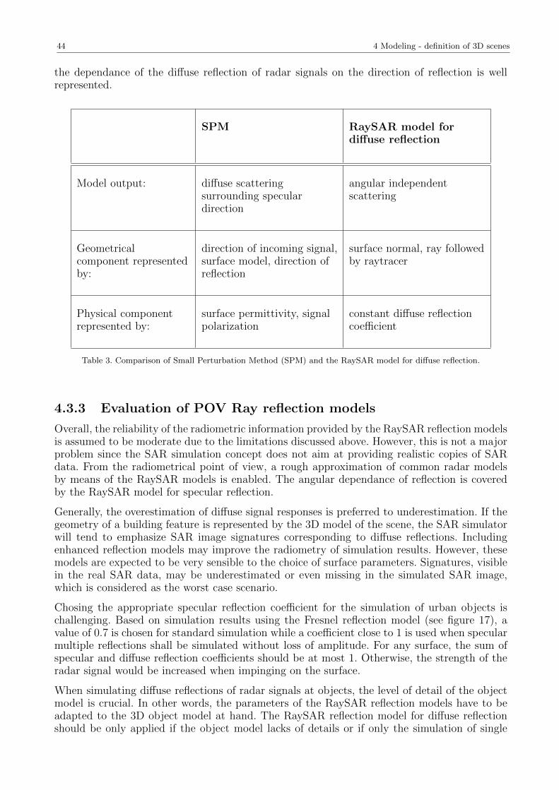
44 4 Modeling - definition of 3D scenes
the dependance of the diffuse reflection of radar signals on the direction of reflection is wellrepresented.
SPM RaySAR model fordiffuse reflection
Model output: diffuse scatteringsurrounding speculardirection
angular independentscattering
Geometricalcomponent representedby:
direction of incoming signal,surface model, direction ofreflection
surface normal, ray followedby raytracer
Physical componentrepresented by:
surface permittivity, signalpolarization
constant diffuse reflectioncoefficient
Table 3. Comparison of Small Perturbation Method (SPM) and the RaySAR model for diffuse reflection.
4.3.3 Evaluation of POV Ray reflection models
Overall, the reliability of the radiometric information provided by the RaySAR reflection modelsis assumed to be moderate due to the limitations discussed above. However, this is not a majorproblem since the SAR simulation concept does not aim at providing realistic copies of SARdata. From the radiometrical point of view, a rough approximation of common radar modelsby means of the RaySAR models is enabled. The angular dependance of reflection is coveredby the RaySAR model for specular reflection.
Generally, the overestimation of diffuse signal responses is preferred to underestimation. If thegeometry of a building feature is represented by the 3D model of the scene, the SAR simulatorwill tend to emphasize SAR image signatures corresponding to diffuse reflections. Includingenhanced reflection models may improve the radiometry of simulation results. However, thesemodels are expected to be very sensible to the choice of surface parameters. Signatures, visiblein the real SAR data, may be underestimated or even missing in the simulated SAR image,which is considered as the worst case scenario.
Chosing the appropriate specular reflection coefficient for the simulation of urban objects ischallenging. Based on simulation results using the Fresnel reflection model (see figure 17), avalue of 0.7 is chosen for standard simulation while a coefficient close to 1 is used when specularmultiple reflections shall be simulated without loss of amplitude. For any surface, the sum ofspecular and diffuse reflection coefficients should be at most 1. Otherwise, the strength of theradar signal would be increased when impinging on the surface.
When simulating diffuse reflections of radar signals at objects, the level of detail of the objectmodel is crucial. In other words, the parameters of the RaySAR reflection models have to beadapted to the 3D object model at hand. The RaySAR reflection model for diffuse reflectionshould be only applied if the object model lacks of details or if only the simulation of single
4.4 Modeling step - summary 45
bounce is of interest. Thereby, the shape of objects represented by flat surfaces can be madevisible in the the azimuth-range plane. Moreover, shadow maps can be provided.
In case of detailed 3D object models, the RaySAR model for specular reflection should beused for the reliable representation of multiple reflections. For VHR SAR systems in X-Band,the expression ’detailed’ is linked to the following precondition: when simulating an object, alltrihedrals having a sidelength of larger than 10 cm have to be represented in the 3D objectmodel. If object surfaces show little roughness compared to the signal wavelength (3.1 cm inX-Band), a rough approximation of the SPM model is enabled. To this end, the roughness pa-rameter of the specular highlight model has to be chosen appropriately for each surface in orderto model the angular dependance of signal reflection. For instance, the diffuse backscatteringdisplayed in figure 18, simulated for bare soil having a surface standard deviation of 0.4 cmand a surface correlation length of 8.4 cm, can be approximated by using a roughness factorof 3.3 · 10−3. When using the SPM, the power densities larger than 0.05 W
m2 cover an angleinterval of approximately 32.8 and 31.6 in HH and VV, respectively. The RaySAR model forspecular reflection yields signal responses covering an angle interval of 32.2. When reducingthe surface standard deviation to 0.1 cm and doubling the surface correlation length of 16.4 cm,the roughness factor may be chosen as 8.5 · 10−4. Then, the SPM power densities larger than0.05 cover an angle interval of 16.5 and 16.3 for HH and VV, respectively. The main lobe ofthe radar signal simulated by the RaySAR model for specular reflection is located within anangle interval of 16.4. Table 4 gives a short summary for the setting of surface parameters inRaySAR. For man-made objects, a constant permittivity of 5.7 + j · 1.3 is chosen for groundsurfaces and buildings.
The simulation of signal interactions with objects and the surrounding ground is not straight-forward. In most cases, the ground has to be represented by a flat plane where no diffuse signalwould be detected when using the parameters given by Table 4. When using the RaySAR modelfor diffuse reflection, the assumption of Lambertian backscattering will cause strong overesti-mation of multiple reflections where ground is involved. A good compromize may be using ahigh roughness value for the reflection model for specular highlights, e.g. 0.3, in combinationwith a decreased specular reflection coefficient, e.g. 0.3, in order to enable direct backscatteringof radar signals from the ground in combination with angle dependent multiple reflections. Inany case, geometrical information is needed for reliable simulation of ground surfaces.
To conclude, any definition of reflection parameters can only provide a rough approximation ofreal signal reflections. Especially, appropriate setting of the reflection coefficients and, hence,the absorbtion of radar signals is hard to be realized. Hence, limitations in the representation ofSAR image radiometry have to be accepted. However, the geometrical component of specularand diffuse reflection of radar signals can be considered. This is of major importance sincethe development of RaySAR is focused on simulating the geometrical distribution of signalresponses.
4.4 Modeling step - summary
In this chapter, the modeling of 3D object scenes has been adressed from three aspects: thedefinition of 3D object models, the definition of the virtual SAR system, and the definition ofradar reflection models.
The modeling of geometrical shapes can be performed in the POV-Ray editor. In contrast,modeling of detailed objects is very time consuming and requires knowledge about the originof data. Hence, when applying RaySAR to real SAR data, the simulation of objects is focusedon available object models of known origin.
The virtual SAR system is represented by an orthographic camera in azimuth and elevation.
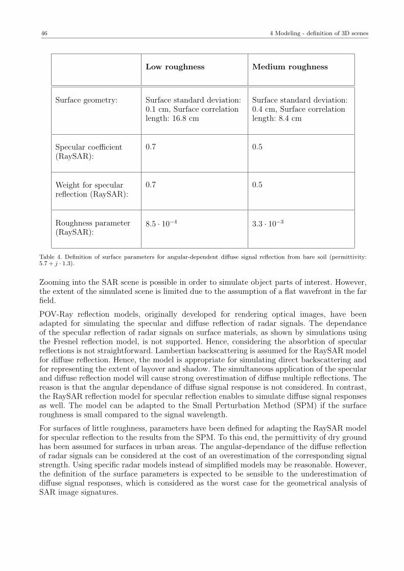
46 4 Modeling - definition of 3D scenes
Low roughness Medium roughness
Surface geometry: Surface standard deviation:0.1 cm, Surface correlationlength: 16.8 cm
Surface standard deviation:0.4 cm, Surface correlationlength: 8.4 cm
Specular coefficient(RaySAR):
0.7 0.5
Weight for specularreflection (RaySAR):
0.7 0.5
Roughness parameter(RaySAR):
8.5 · 10−4 3.3 · 10−3
Table 4. Definition of surface parameters for angular-dependent diffuse signal reflection from bare soil (permittivity:5.7 + j · 1.3).
Zooming into the SAR scene is possible in order to simulate object parts of interest. However,the extent of the simulated scene is limited due to the assumption of a flat wavefront in the farfield.
POV-Ray reflection models, originally developed for rendering optical images, have beenadapted for simulating the specular and diffuse reflection of radar signals. The dependanceof the specular reflection of radar signals on surface materials, as shown by simulations usingthe Fresnel reflection model, is not supported. Hence, considering the absorbtion of specularreflections is not straightforward. Lambertian backscattering is assumed for the RaySAR modelfor diffuse reflection. Hence, the model is appropriate for simulating direct backscattering andfor representing the extent of layover and shadow. The simultaneous application of the specularand diffuse reflection model will cause strong overestimation of diffuse multiple reflections. Thereason is that the angular dependance of diffuse signal response is not considered. In contrast,the RaySAR reflection model for specular reflection enables to simulate diffuse signal responsesas well. The model can be adapted to the Small Perturbation Method (SPM) if the surfaceroughness is small compared to the signal wavelength.
For surfaces of little roughness, parameters have been defined for adapting the RaySAR modelfor specular reflection to the results from the SPM. To this end, the permittivity of dry groundhas been assumed for surfaces in urban areas. The angular-dependance of the diffuse reflectionof radar signals can be considered at the cost of an overestimation of the corresponding signalstrength. Using specific radar models instead of simplified models may be reasonable. However,the definition of the surface parameters is expected to be sensible to the underestimation ofdiffuse signal responses, which is considered as the worst case for the geometrical analysis ofSAR image signatures.
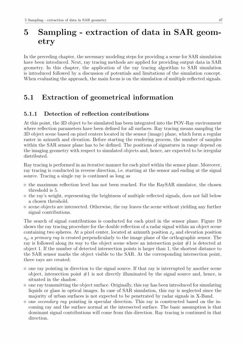
5 Sampling - extraction of data in SAR geometry 47
5 Sampling - extraction of data in SAR geom-etry
In the preceding chapter, the necessary modeling steps for providing a scene for SAR simulationhave been introduced. Next, ray tracing methods are applied for providing output data in SARgeometry. In this chapter, the application of the ray tracing algorithm to SAR simulationis introduced followed by a discussion of potentials and limitations of the simulation concept.When evaluating the approach, the main focus is on the simulation of multiple reflected signals.
5.1 Extraction of geometrical information
5.1.1 Detection of reflection contributions
At this point, the 3D object to be simulated has been integrated into the POV-Ray environmentwhere reflection parameters have been defined for all surfaces. Ray tracing means sampling the3D object scene based on pixel centers located in the sensor (image) plane, which form a regularraster in azimuth and elevation. Before starting the rendering process, the number of sampleswithin the SAR sensor plane has to be defined. The positions of signatures in range depend onthe imaging geometry with respect to simulated objects and, hence, are expected to be irregulardistributed.
Ray tracing is performed in an iterative manner for each pixel within the sensor plane. Moreover,ray tracing is conducted in reverse direction, i.e. starting at the sensor and ending at the signalsource. Tracing a single ray is continued as long as
the maximum reflection level has not been reached. For the RaySAR simulator, the chosenthreshold is 5. the ray’s weight, representing the brightness of multiple reflected signals, does not fall below
a chosen threshold. scene objects are intersected. Otherwise, the ray leaves the scene without yielding any further
signal contributions.
The search of signal contributions is conducted for each pixel in the sensor plane. Figure 19shows the ray tracing procedure for the double reflection of a radar signal within an object scenecontaining two spheres. At a pixel center, located at azimuth position xp and elevation positionsp, a primary ray is created perpendicularly to the image plane of the orthographic sensor. Theray is followed along its way to the object scene where an intersection point #1 is detected atobject 1. If the number of detected intersection points is larger than 1, the shortest distance tothe SAR sensor marks the object visible to the SAR. At the corresponding intersection point,three rays are created:
one ray pointing in direction to the signal source. If that ray is interrupted by another sceneobject, intersection point #1 is not directly illuminated by the signal source and, hence, issituated in the shadow. one ray transmitting the object surface. Originally, this ray has been introduced for simulating
liquids or glass in optical images. In case of SAR simulation, this ray is neglected since themajority of urban surfaces is not expected to be penetrated by radar signals in X-Band. one secondary ray pointing in specular direction. This ray is constructed based on the in-
coming ray and the surface normal at the intersected surface. The basic assumption is thatdominant signal contributions will come from this direction. Ray tracing is continued in thatdirection.
48 5 Sampling - extraction of data in SAR geometry
Fig. 19. Localization of signal contributions by means of RaySAR for the double reflection of a radar signal. Rays arefollowed in reverse direction (r1 → r2 → r3), i.e. starting at the SAR sensor and ending at the SAR antenna.
If intersection point #1 is situated in the shadow, no signal is detected. Otherwise, the signalamplitude is calculated using the RaySAR reflection models described in chapter 4.3. Further-more, a decision is made whether the current reflection process at the intersection point #1 isof type ’specular’ or not. To this end, the reflection geometry at intersection point 1 is analyzed(see chapter 5.1.4). Eventually, the 3D coordinates of a radar signal backscattered from object#1 are:
xs = xp
rs = r1
ss = sp
(16)
The search for a double reflected signal is started by following the secondary ray which intersectsobject 2 (intersection point #2). Again, a shadow test is conducted. Given the SAR antenna assignal source, the amplitude of the signal reflected in direction of the secondary ray is calculatedand weighted using the reflection coefficient assigned to object 1. The analysis for specular/non-specular reflection is performed locally at intersection point #2 since the secondary ray hasbeen already defined in specular direction. For providing the coordinates of the double bounceprocess, a ray parallel to the primary ray has to be created at intersection point #2. In thefollowing, this ray is referred to as focusing ray. The intersection point between the focusing rayand the planar signal source determines the origin of the radar signal at the virtual SAR and isfound in the world coordinate system of the simulated object model. This point is not relatedto the antenna of a real SAR system (see chapter 4.2). Instead, the signal origin is a mean forsimulating the 3D position of multiple reflected radar signals. To this end, the coordinates of thesignal origin are transformed into the image coordinate system of the virtual sensor (see crossat x0 and s0 in figure 19), what is possible due to the known sensor position and line-of-sight.Thereafter, the azimuth, range, and elevation coordinate of the double reflected radar signal isderived by
xs =x0 + xp
2(17)
5.1 Extraction of geometrical information 49
rs =r1 + r2 + r3
2(18)
ss =s0 + sp
2(19)
A detailed discussion of these equations is provided in chapter 5.1.2 and 5.1.3. The search fortriple reflections is continued after the definition of a new secondary ray at intersection point#2, which is not displayed in figure 19. In case of an intersected object, another focusing ray isneeded for finding the coordinates of the triple bounce signal. Eventually, output informationis gathered for each detected radar signal and stored in a signal vector, which is
Ss =[xs rs ss As bs fs Xi Yi Zi
](20)
where
xs, rs, and ss describe the position of the signal phase center. As is the amplitude of the detected signal [normalized value between 0 and 1]. bs is the bounce level corresponding to the detected signal, e.g. 1 in case of single bounce. fs is a flag for marking specular reflections [0 for non-specular, 1 for specular] (see chapter
5.1.4). Xi, Yi, and Zi are the coordinates of the detected intersection point. The position of the point
is captured optionally in order to identify the reflecting surfaces contributing to a salient SARimage signature (see chapter 6.4.2).
In case of n signal contributions, Ss is extended to a signal matrix of size n x 6 where differentsignal contributions are organized in rows.
RaySAR simulates a non-squinted SAR. For direct backscattering from objects, the signalresponse is found at the zero doppler position along the synthetic aperture. Instead of simulatingthe spatial resolution of signatures, only the position of the amplitude peak is simulated in theazimuth-range plane. Hence, the geometrical resolution of the virtual SAR system is infinite,i.e. a trihedral is focused at one point in space. By purpose, the dependance of SAR products onthe number and distribution of samples or the length of the synthetic aperture in azimuth andelevation is not considered. In contrast, phase centers are directly simulated assuming a staticSAR system. Discrete sampling by means of the ray tracer enables the simulation of analyticalshapes, e.g. a sphere defined by one point and a radius, but also causes disadvantages. Signalcontributions are represented by vector data which have to be rasterized in order to provideSAR images. Since the ray tracer can be considered as a kind of scanner, the spatial resolutionof the SAR simulator has to be chosen appropriately. In this context, the expression ’spatialresolution’ refers to the level of object detail represented by the resulting point cloud (Lichti,2004). While surface information is well represented by means of point patterns, the simulationof edges is moderate due to discrete sampling of a continuous structure.
The simulation of detailed 3D models is enabled by neglecting physical effects affecting thesignal interaction with objects, such as signal diffraction at edges or creeping waves on metallicsurfaces. However, for signals in X-Band, these effects are expected to be much weaker thanspecular reflections, which are of main interest in this thesis. Moreover, the majority of sig-nal reflections are expected to occur in the optics region (object size > 10 times the signalwavelength) where physical surface effects are minimal (Knott et al., 2004).
5.1.2 Focusing in azimuth
Real SAR data are derived by processing raw data captured along the synthetic aperture inazimuth. The corresponding processing effects have to be accounted for when simulating the
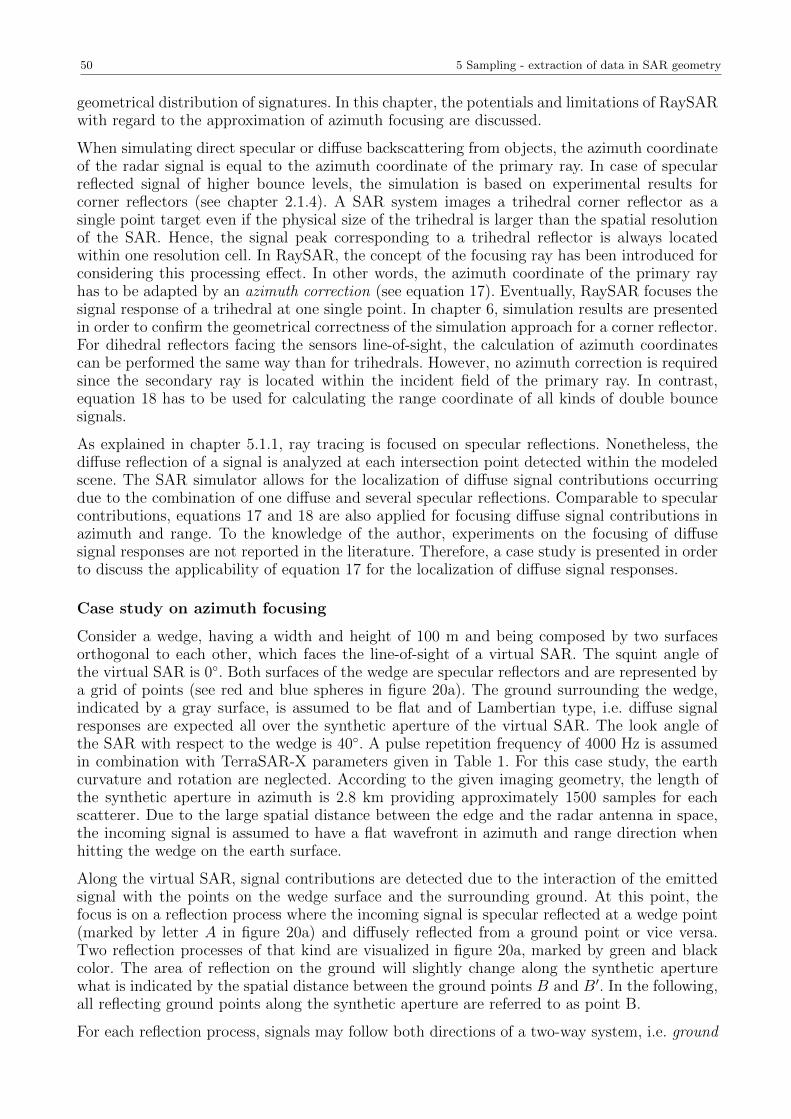
50 5 Sampling - extraction of data in SAR geometry
geometrical distribution of signatures. In this chapter, the potentials and limitations of RaySARwith regard to the approximation of azimuth focusing are discussed.
When simulating direct specular or diffuse backscattering from objects, the azimuth coordinateof the radar signal is equal to the azimuth coordinate of the primary ray. In case of specularreflected signal of higher bounce levels, the simulation is based on experimental results forcorner reflectors (see chapter 2.1.4). A SAR system images a trihedral corner reflector as asingle point target even if the physical size of the trihedral is larger than the spatial resolutionof the SAR. Hence, the signal peak corresponding to a trihedral reflector is always locatedwithin one resolution cell. In RaySAR, the concept of the focusing ray has been introduced forconsidering this processing effect. In other words, the azimuth coordinate of the primary rayhas to be adapted by an azimuth correction (see equation 17). Eventually, RaySAR focuses thesignal response of a trihedral at one single point. In chapter 6, simulation results are presentedin order to confirm the geometrical correctness of the simulation approach for a corner reflector.For dihedral reflectors facing the sensors line-of-sight, the calculation of azimuth coordinatescan be performed the same way than for trihedrals. However, no azimuth correction is requiredsince the secondary ray is located within the incident field of the primary ray. In contrast,equation 18 has to be used for calculating the range coordinate of all kinds of double bouncesignals.
As explained in chapter 5.1.1, ray tracing is focused on specular reflections. Nonetheless, thediffuse reflection of a signal is analyzed at each intersection point detected within the modeledscene. The SAR simulator allows for the localization of diffuse signal contributions occurringdue to the combination of one diffuse and several specular reflections. Comparable to specularcontributions, equations 17 and 18 are also applied for focusing diffuse signal contributions inazimuth and range. To the knowledge of the author, experiments on the focusing of diffusesignal responses are not reported in the literature. Therefore, a case study is presented in orderto discuss the applicability of equation 17 for the localization of diffuse signal responses.
Case study on azimuth focusing
Consider a wedge, having a width and height of 100 m and being composed by two surfacesorthogonal to each other, which faces the line-of-sight of a virtual SAR. The squint angle ofthe virtual SAR is 0. Both surfaces of the wedge are specular reflectors and are represented bya grid of points (see red and blue spheres in figure 20a). The ground surrounding the wedge,indicated by a gray surface, is assumed to be flat and of Lambertian type, i.e. diffuse signalresponses are expected all over the synthetic aperture of the virtual SAR. The look angle ofthe SAR with respect to the wedge is 40. A pulse repetition frequency of 4000 Hz is assumedin combination with TerraSAR-X parameters given in Table 1. For this case study, the earthcurvature and rotation are neglected. According to the given imaging geometry, the length ofthe synthetic aperture in azimuth is 2.8 km providing approximately 1500 samples for eachscatterer. Due to the large spatial distance between the edge and the radar antenna in space,the incoming signal is assumed to have a flat wavefront in azimuth and range direction whenhitting the wedge on the earth surface.
Along the virtual SAR, signal contributions are detected due to the interaction of the emittedsignal with the points on the wedge surface and the surrounding ground. At this point, thefocus is on a reflection process where the incoming signal is specular reflected at a wedge point(marked by letter A in figure 20a) and diffusely reflected from a ground point or vice versa.Two reflection processes of that kind are visualized in figure 20a, marked by green and blackcolor. The area of reflection on the ground will slightly change along the synthetic aperturewhat is indicated by the spatial distance between the ground points B and B′. In the following,all reflecting ground points along the synthetic aperture are referred to as point B.
For each reflection process, signals may follow both directions of a two-way system, i.e. ground
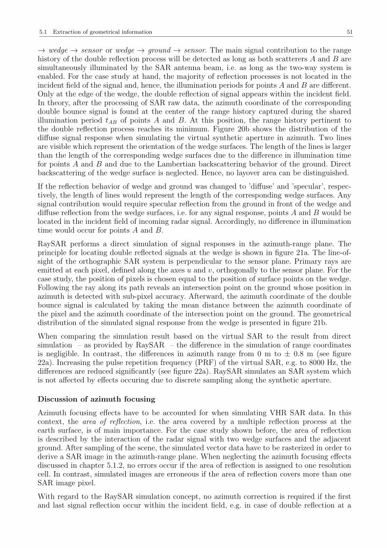
5.1 Extraction of geometrical information 51
→ wedge → sensor or wedge → ground → sensor. The main signal contribution to the rangehistory of the double reflection process will be detected as long as both scatterers A and B aresimultaneously illuminated by the SAR antenna beam, i.e. as long as the two-way system isenabled. For the case study at hand, the majority of reflection processes is not located in theincident field of the signal and, hence, the illumination periods for points A and B are different.Only at the edge of the wedge, the double reflection of signal appears within the incident field.In theory, after the processing of SAR raw data, the azimuth coordinate of the correspondingdouble bounce signal is found at the center of the range history captured during the sharedillumination period tAB of points A and B. At this position, the range history pertinent tothe double reflection process reaches its minimum. Figure 20b shows the distribution of thediffuse signal response when simulating the virtual synthetic aperture in azimuth. Two linesare visible which represent the orientation of the wedge surfaces. The length of the lines is largerthan the length of the corresponding wedge surfaces due to the difference in illumination timefor points A and B and due to the Lambertian backscattering behavior of the ground. Directbackscattering of the wedge surface is neglected. Hence, no layover area can be distinguished.
If the reflection behavior of wedge and ground was changed to ’diffuse’ and ’specular’, respec-tively, the length of lines would represent the length of the corresponding wedge surfaces. Anysignal contribution would require specular reflection from the ground in front of the wedge anddiffuse reflection from the wedge surfaces, i.e. for any signal response, points A and B would belocated in the incident field of incoming radar signal. Accordingly, no difference in illuminationtime would occur for points A and B.
RaySAR performs a direct simulation of signal responses in the azimuth-range plane. Theprinciple for locating double reflected signals at the wedge is shown in figure 21a. The line-of-sight of the orthographic SAR system is perpendicular to the sensor plane. Primary rays areemitted at each pixel, defined along the axes u and v, orthogonally to the sensor plane. For thecase study, the position of pixels is chosen equal to the position of surface points on the wedge.Following the ray along its path reveals an intersection point on the ground whose position inazimuth is detected with sub-pixel accuracy. Afterward, the azimuth coordinate of the doublebounce signal is calculated by taking the mean distance between the azimuth coordinate ofthe pixel and the azimuth coordinate of the intersection point on the ground. The geometricaldistribution of the simulated signal response from the wedge is presented in figure 21b.
When comparing the simulation result based on the virtual SAR to the result from directsimulation – as provided by RaySAR – the difference in the simulation of range coordinatesis negligible. In contrast, the differences in azimuth range from 0 m to ± 0.8 m (see figure22a). Increasing the pulse repetition frequency (PRF) of the virtual SAR, e.g. to 8000 Hz, thedifferences are reduced significantly (see figure 22a). RaySAR simulates an SAR system whichis not affected by effects occuring due to discrete sampling along the synthetic aperture.
Discussion of azimuth focusing
Azimuth focusing effects have to be accounted for when simulating VHR SAR data. In thiscontext, the area of reflection, i.e. the area covered by a multiple reflection process at theearth surface, is of main importance. For the case study shown before, the area of reflectionis described by the interaction of the radar signal with two wedge surfaces and the adjacentground. After sampling of the scene, the simulated vector data have to be rasterized in order toderive a SAR image in the azimuth-range plane. When neglecting the azimuth focusing effectsdiscussed in chapter 5.1.2, no errors occur if the area of reflection is assigned to one resolutioncell. In contrast, simulated images are erroneous if the area of reflection covers more than oneSAR image pixel.
With regard to the RaySAR simulation concept, no azimuth correction is required if the firstand last signal reflection occur within the incident field, e.g. in case of double reflection at a
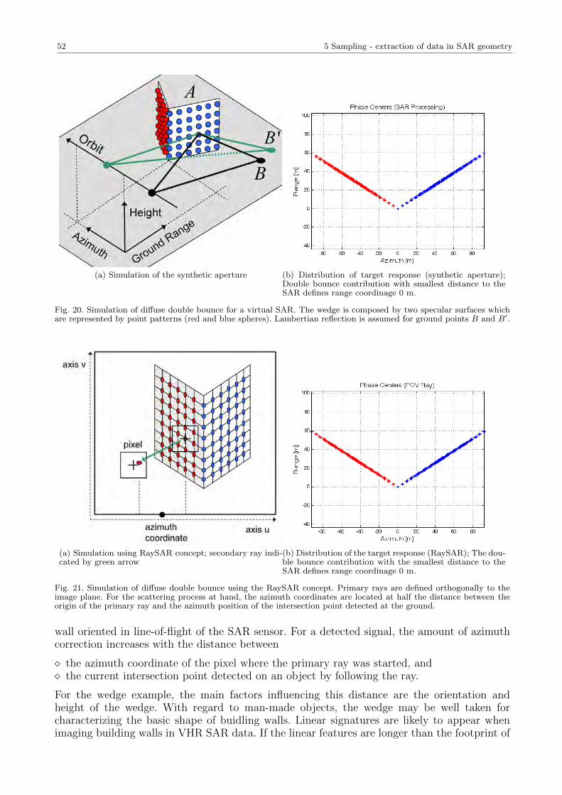
52 5 Sampling - extraction of data in SAR geometry
(a) Simulation of the synthetic aperture (b) Distribution of target response (synthetic aperture);Double bounce contribution with smallest distance to theSAR defines range coordinage 0 m.
Fig. 20. Simulation of diffuse double bounce for a virtual SAR. The wedge is composed by two specular surfaces whichare represented by point patterns (red and blue spheres). Lambertian reflection is assumed for ground points B and B′.
(a) Simulation using RaySAR concept; secondary ray indi-cated by green arrow
(b) Distribution of the target response (RaySAR); The dou-ble bounce contribution with the smallest distance to theSAR defines range coordinage 0 m.
Fig. 21. Simulation of diffuse double bounce using the RaySAR concept. Primary rays are defined orthogonally to theimage plane. For the scattering process at hand, the azimuth coordinates are located at half the distance between theorigin of the primary ray and the azimuth position of the intersection point detected at the ground.
wall oriented in line-of-flight of the SAR sensor. For a detected signal, the amount of azimuthcorrection increases with the distance between
the azimuth coordinate of the pixel where the primary ray was started, and the current intersection point detected on an object by following the ray.
For the wedge example, the main factors influencing this distance are the orientation andheight of the wedge. With regard to man-made objects, the wedge may be well taken forcharacterizing the basic shape of buidling walls. Linear signatures are likely to appear whenimaging building walls in VHR SAR data. If the linear features are longer than the footprint of
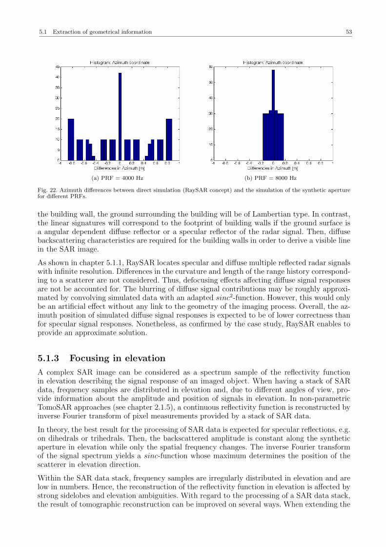
5.1 Extraction of geometrical information 53
(a) PRF = 4000 Hz (b) PRF = 8000 Hz
Fig. 22. Azimuth differences between direct simulation (RaySAR concept) and the simulation of the synthetic aperturefor different PRFs.
the building wall, the ground surrounding the building will be of Lambertian type. In contrast,the linear signatures will correspond to the footprint of building walls if the ground surface isa angular dependent diffuse reflector or a specular reflector of the radar signal. Then, diffusebackscattering characteristics are required for the building walls in order to derive a visible linein the SAR image.
As shown in chapter 5.1.1, RaySAR locates specular and diffuse multiple reflected radar signalswith infinite resolution. Differences in the curvature and length of the range history correspond-ing to a scatterer are not considered. Thus, defocusing effects affecting diffuse signal responsesare not be accounted for. The blurring of diffuse signal contributions may be roughly approxi-mated by convolving simulated data with an adapted sinc2-function. However, this would onlybe an artificial effect without any link to the geometry of the imaging process. Overall, the az-imuth position of simulated diffuse signal responses is expected to be of lower correctness thanfor specular signal responses. Nonetheless, as confirmed by the case study, RaySAR enables toprovide an approximate solution.
5.1.3 Focusing in elevation
A complex SAR image can be considered as a spectrum sample of the reflectivity functionin elevation describing the signal response of an imaged object. When having a stack of SARdata, frequency samples are distributed in elevation and, due to different angles of view, pro-vide information about the amplitude and position of signals in elevation. In non-parametricTomoSAR approaches (see chapter 2.1.5), a continuous reflectivity function is reconstructed byinverse Fourier transform of pixel measurements provided by a stack of SAR data.
In theory, the best result for the processing of SAR data is expected for specular reflections, e.g.on dihedrals or trihedrals. Then, the backscattered amplitude is constant along the syntheticaperture in elevation while only the spatial frequency changes. The inverse Fourier transformof the signal spectrum yields a sinc-function whose maximum determines the position of thescatterer in elevation direction.
Within the SAR data stack, frequency samples are irregularly distributed in elevation and arelow in numbers. Hence, the reconstruction of the reflectivity function in elevation is affected bystrong sidelobes and elevation ambiguities. With regard to the processing of a SAR data stack,the result of tomographic reconstruction can be improved on several ways. When extending the
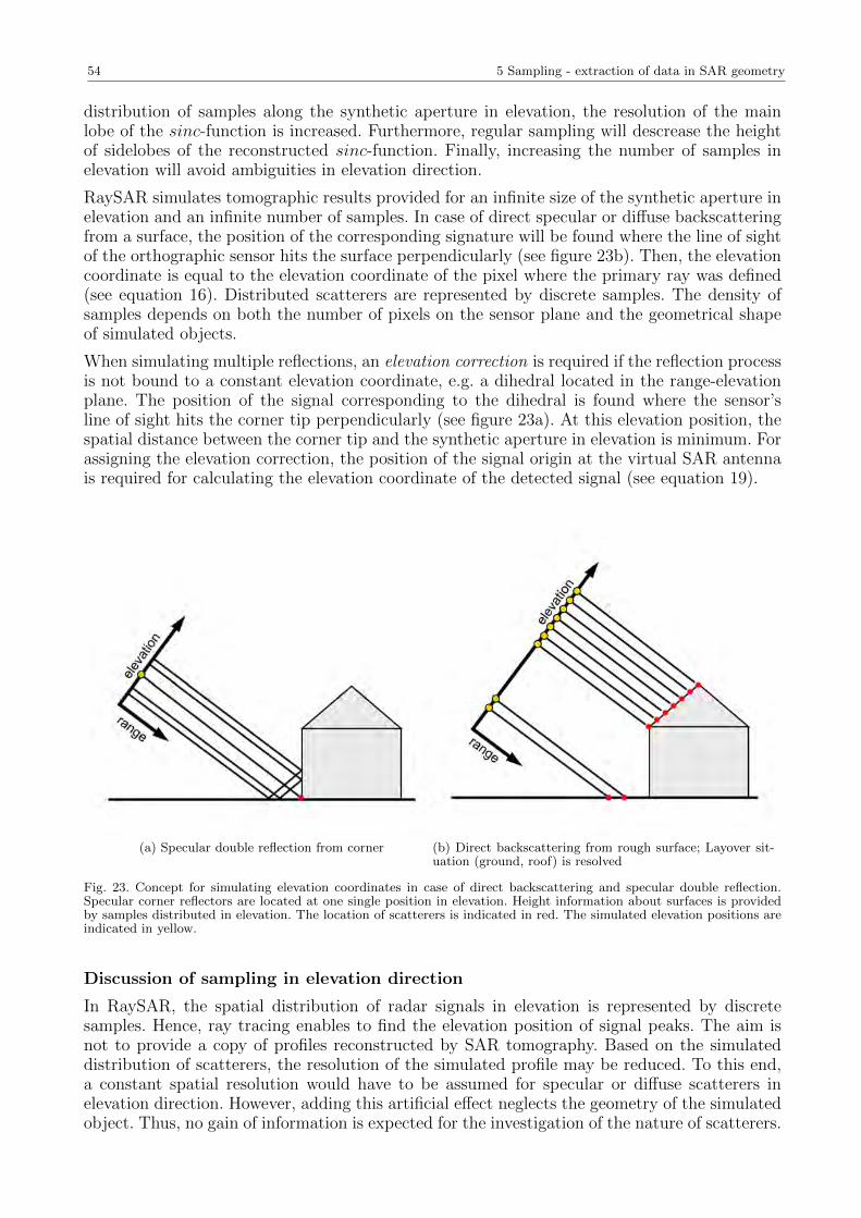
54 5 Sampling - extraction of data in SAR geometry
distribution of samples along the synthetic aperture in elevation, the resolution of the mainlobe of the sinc-function is increased. Furthermore, regular sampling will descrease the heightof sidelobes of the reconstructed sinc-function. Finally, increasing the number of samples inelevation will avoid ambiguities in elevation direction.
RaySAR simulates tomographic results provided for an infinite size of the synthetic aperture inelevation and an infinite number of samples. In case of direct specular or diffuse backscatteringfrom a surface, the position of the corresponding signature will be found where the line of sightof the orthographic sensor hits the surface perpendicularly (see figure 23b). Then, the elevationcoordinate is equal to the elevation coordinate of the pixel where the primary ray was defined(see equation 16). Distributed scatterers are represented by discrete samples. The density ofsamples depends on both the number of pixels on the sensor plane and the geometrical shapeof simulated objects.
When simulating multiple reflections, an elevation correction is required if the reflection processis not bound to a constant elevation coordinate, e.g. a dihedral located in the range-elevationplane. The position of the signal corresponding to the dihedral is found where the sensor’sline of sight hits the corner tip perpendicularly (see figure 23a). At this elevation position, thespatial distance between the corner tip and the synthetic aperture in elevation is minimum. Forassigning the elevation correction, the position of the signal origin at the virtual SAR antennais required for calculating the elevation coordinate of the detected signal (see equation 19).
(a) Specular double reflection from corner (b) Direct backscattering from rough surface; Layover sit-uation (ground, roof) is resolved
Fig. 23. Concept for simulating elevation coordinates in case of direct backscattering and specular double reflection.Specular corner reflectors are located at one single position in elevation. Height information about surfaces is providedby samples distributed in elevation. The location of scatterers is indicated in red. The simulated elevation positions areindicated in yellow.
Discussion of sampling in elevation direction
In RaySAR, the spatial distribution of radar signals in elevation is represented by discretesamples. Hence, ray tracing enables to find the elevation position of signal peaks. The aim isnot to provide a copy of profiles reconstructed by SAR tomography. Based on the simulateddistribution of scatterers, the resolution of the simulated profile may be reduced. To this end,a constant spatial resolution would have to be assumed for specular or diffuse scatterers inelevation direction. However, adding this artificial effect neglects the geometry of the simulatedobject. Thus, no gain of information is expected for the investigation of the nature of scatterers.
5.2 Evaluation of the simulation of multiple reflections 55
Signal responses directly backscattered from objects are regularly distributed in the azimuth-elevation plane. In contrast, multiple reflections may be irregularly distributed due to the needfor an elevation correction. For obtaining a reflectivity profile in elevation, a rasterization stepis needed (see chapter 6.3). The localization of directly backscattered signals in elevation ishelpful for resolving layover situations at man-made objects (see figure 23b). Furthermore, theinterpretion of scatterers is supported since the spatial distribution of single bounce contribu-tions provides information about the geometrical shape of objects. Specular multiple reflectionsat dihedrals or trihedrals are located at one single point in elevation. Thus, point scatterersspatially distributed in elevation can be separated for each resolution cell.
Comparable to the azimuth direction, the correctness of the localization of diffuse reflectedsignals is lower than for specular reflected signals. However, the resulting elevation positionof diffuse signal responses is expected to be close to reality. In chapter 6.3, basic shapes aresimulated by RaySAR. To this end, the output data provided by the ray tracer are exploitedin order to analyze signal responses in elevation direction. In this context, the functionality ofthe simulation in elevation direction is verified by simulation results for a corner reflector.
5.1.4 Detection of specular reflections
In RaySAR, the simulation of SAR image radiometry is limited due to simplified reflectionmodels. Additional information may be helpful for interpreting salient signatures in real SARdata which are not appropriately represented by the simulated map. To this end, a geometricalanalysis of signal reflections, applied during the sampling of the modeled scene, enables to detectspecular reflections at dihedrals, trihedrals or other structures. Rays only following speculardirections on their way from the signal source to the sensor are marked by a flag value. Infigure 24, the basic concept for the geometrical analysis is visualized. Tracing a ray starts atthe center of an image pixel within the sensor plane. The primary ray ~R, intersecting the sensorplane orthogonally, is followed and an intersection point P is detected on an object surface. Atthis position, a virtual ray ~S is defined in specular direction based on the surface normal ~Nand the incoming ray ~R by
~S = ~R− 2 ~N · ( ~N · ~R) (21)
Vector ~L, pointing in direction to the signal source, and vector ~S define a scalar angle which is
cos(α) =∣∣∣~S · ~L∣∣∣ (22)
If α is smaller than a defined threshold ∆α, which is 1, the signal reflection is classified as’specular’. Then, the default flag value is changed from 0 to 1. Since the geometrical analysis isconducted for all primary and secondary rays, one flag value is defined for each signal responsedetected in the simulated scene. In figure 24, an example for diffuse reflection is given sincevector ~L is not situated in the cone defined by vector ~S and angle ∆α.
5.2 Evaluation of the simulation of multiple reflections
In this chapter, the potentials and limitations of ray tracing with regard to the simulation ofmultiple reflections are discussed. The need for the discussion is based on the fact that, tothe knowledge of the author, a thorough evaluation of the applicability of ray tracing for thesimulation of multiple reflections of radar signals is not reported in the literature. Generally, the
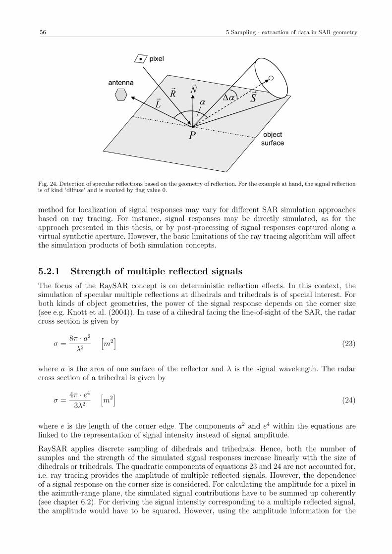
56 5 Sampling - extraction of data in SAR geometry
Fig. 24. Detection of specular reflections based on the geometry of reflection. For the example at hand, the signal reflectionis of kind ’diffuse’ and is marked by flag value 0.
method for localization of signal responses may vary for different SAR simulation approachesbased on ray tracing. For instance, signal responses may be directly simulated, as for theapproach presented in this thesis, or by post-processing of signal responses captured along avirtual synthetic aperture. However, the basic limitations of the ray tracing algorithm will affectthe simulation products of both simulation concepts.
5.2.1 Strength of multiple reflected signals
The focus of the RaySAR concept is on deterministic reflection effects. In this context, thesimulation of specular multiple reflections at dihedrals and trihedrals is of special interest. Forboth kinds of object geometries, the power of the signal response depends on the corner size(see e.g. Knott et al. (2004)). In case of a dihedral facing the line-of-sight of the SAR, the radarcross section is given by
σ =8π · a2
λ2
[m2]
(23)
where a is the area of one surface of the reflector and λ is the signal wavelength. The radarcross section of a trihedral is given by
σ =4π · e4
3λ2
[m2]
(24)
where e is the length of the corner edge. The components a2 and e4 within the equations arelinked to the representation of signal intensity instead of signal amplitude.
RaySAR applies discrete sampling of dihedrals and trihedrals. Hence, both the number ofsamples and the strength of the simulated signal responses increase linearly with the size ofdihedrals or trihedrals. The quadratic components of equations 23 and 24 are not accounted for,i.e. ray tracing provides the amplitude of multiple reflected signals. However, the dependenceof a signal response on the corner size is considered. For calculating the amplitude for a pixel inthe azimuth-range plane, the simulated signal contributions have to be summed up coherently(see chapter 6.2). For deriving the signal intensity corresponding to a multiple reflected signal,the amplitude would have to be squared. However, using the amplitude information for the
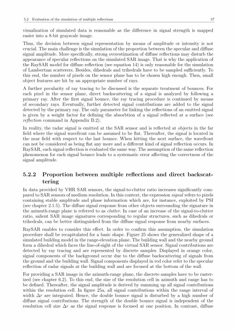
5.2 Evaluation of the simulation of multiple reflections 57
visualization of simulated data is reasonable as the difference in signal strength is mappedeasier into a 8-bit grayscale image.
Thus, the decision between signal representation by means of amplitude or intensity is notcrucial. The main challenge is the simulation of the proportion between the specular and diffusesignal amplitude. More specifically, strong overestimation of diffuse reflections may disturb theappearance of specular reflections on the simulated SAR image. That is why the application ofthe RaySAR model for diffuse reflection (see equation 14) is only reasonable for the simulationof Lambertian scatterers. Besides, dihedrals and trihedrals have to be sampled sufficiently. Tothis end, the number of pixels on the sensor plane has to be chosen high enough. Then, smallobject features are hit by an appropriate number of rays.
A further pecularity of ray tracing to be discussed is the separate treatment of bounces. Foreach pixel in the sensor plane, direct backscattering of a signal is analyzed by following aprimary ray. After the first signal bounce, the ray tracing procedure is continued by meansof secondary rays. Eventually, further detected signal contributions are added to the signaldetected by the primary ray. The only parameter for linking the reflections of an emitted signalis given by a weight factor for defining the absorbtion of a signal reflected at a surface (seereflection command in Appendix B.2).
In reality, the radar signal is emitted at the SAR sensor and is reflected at objects in the farfield where the signal wavefront can be assumed to be flat. Thereafter, the signal is located inthe near field with respect to the last bounce. When hitting the next surface, the wavefrontcan not be considered as being flat any more and a different kind of signal reflection occurs. InRaySAR, each signal reflection is evaluated the same way. The assumption of the same reflectionphenomenon for each signal bounce leads to a systematic error affecting the correctness of thesignal amplitude.
5.2.2 Proportion between multiple reflections and direct backscat-tering
In data provided by VHR SAR sensors, the signal-to-clutter ratio increases significantly com-pared to SAR sensors of medium resolution. In this context, the expression signal refers to pixelscontaining stable amplitude and phase information which are, for instance, exploited by PSI(see chapter 2.1.5). The diffuse signal response from other objects surrounding the signature inthe azimuth-range plane is referred to as clutter. In case of an increase of the signal-to-clutterratio, salient SAR image signatures corresponding to regular structures, such as dihedrals ortrihedrals, can be better distinguished from the diffuse signal response from nearby surfaces.
RaySAR enables to consider this effect. In order to confirm this assumption, the simulationprocedure shall be recapitulated for a basic shape. Figure 25 shows the generalized shape of asimulated building model in the range-elevation plane. The building wall and the nearby groundform a dihedral which faces the line-of-sight of the virtual SAR sensor. Signal contributions aredetected by ray tracing and are represented by discrete samples. Displayed in orange color,signal components of the background occur due to the diffuse backscattering of signals fromthe ground and the building wall. Signal components displayed in red color refer to the specularreflection of radar signals at the building wall and are focused at the bottom of the wall.
For providing a SAR image in the azimuth-range plane, the discrete samples have to be raster-ized (see chapter 6.2). To this end, the size of the resolution cell in azimuth and range has tobe defined. Thereafter, the signal amplitude is derived by summing up all signal contributionswithin the resolution cell. In figure 25a, all signal contributions within the range interval ofwidth ∆r are integrated. Hence, the double bounce signal is disturbed by a high number ofdiffuse signal contributions. The strength of the double bounce signal is independent of theresolution cell size ∆r as the signal response is focused at one position. In contrast, diffuse
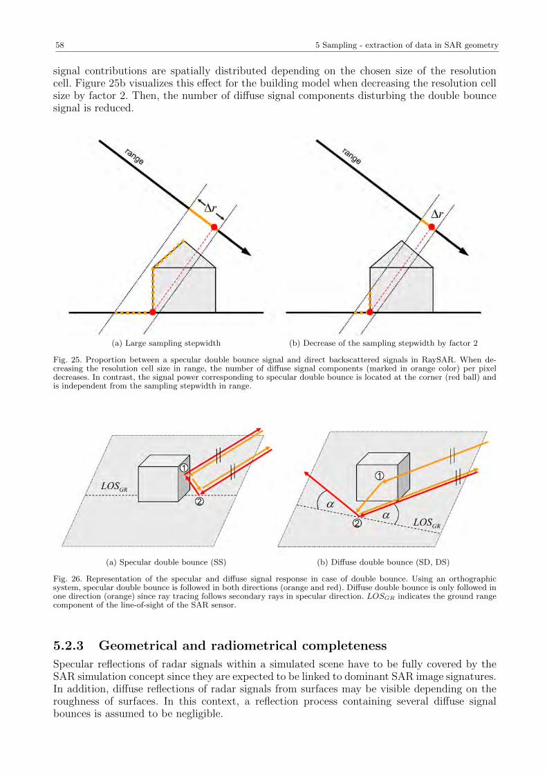
58 5 Sampling - extraction of data in SAR geometry
signal contributions are spatially distributed depending on the chosen size of the resolutioncell. Figure 25b visualizes this effect for the building model when decreasing the resolution cellsize by factor 2. Then, the number of diffuse signal components disturbing the double bouncesignal is reduced.
(a) Large sampling stepwidth (b) Decrease of the sampling stepwidth by factor 2
Fig. 25. Proportion between a specular double bounce signal and direct backscattered signals in RaySAR. When de-creasing the resolution cell size in range, the number of diffuse signal components (marked in orange color) per pixeldecreases. In contrast, the signal power corresponding to specular double bounce is located at the corner (red ball) andis independent from the sampling stepwidth in range.
(a) Specular double bounce (SS) (b) Diffuse double bounce (SD, DS)
Fig. 26. Representation of the specular and diffuse signal response in case of double bounce. Using an orthographicsystem, specular double bounce is followed in both directions (orange and red). Diffuse double bounce is only followed inone direction (orange) since ray tracing follows secondary rays in specular direction. LOSGR indicates the ground rangecomponent of the line-of-sight of the SAR sensor.
5.2.3 Geometrical and radiometrical completeness
Specular reflections of radar signals within a simulated scene have to be fully covered by theSAR simulation concept since they are expected to be linked to dominant SAR image signatures.In addition, diffuse reflections of radar signals from surfaces may be visible depending on theroughness of surfaces. In this context, a reflection process containing several diffuse signalbounces is assumed to be negligible.
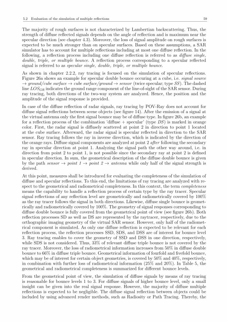
5.2 Evaluation of the simulation of multiple reflections 59
The majority of rough surfaces is not characterized by Lambertian backscattering. Thus, thestrength of diffuse reflected signals depends on the angle of reflection and is maximum near thespecular direction (see chapter 4.3). Moreover, the loss of signal amplitude on rough surfaces isexpected to be much stronger than on specular surfaces. Based on these assumptions, a SARsimulator has to account for multiple reflections including at most one diffuse reflection. In thefollowing, a reflection process including one diffuse reflection is referred to as diffuse single,double, triple, or multiple bounce. A reflection process corresponding to a specular reflectedsignal is referred to as specular single, double, triple, or multiple bounce.
As shown in chapter 2.2.2, ray tracing is focused on the simulation of specular reflections.Figure 26a shows an example for specular double bounce occuring at a cube, i.e. signal source→ ground/cube surface→ cube surface/ground→ sensor (twice specular; type SS ). The dashedline LOSGR indicates the ground range component of the line-of-sight of the SAR sensor. Duringray tracing, both directions of the two-way system are analyzed. Hence, the position and theamplitude of the signal response is provided.
In case of the diffuse reflection of radar signals, ray tracing by POV-Ray does not account fordiffuse signal reflections between scene objects (see figure 14). After the emission of a signal atthe virtual antenna only the first signal bounce may be of diffuse type. In figure 26b, an examplefor a reflection process of the combination ’diffuse + specular’ (type DS ) is marked in orangecolor. First, the radar signal is diffusely scattered at point 2 in direction to point 1 locatedat the cube surface. Afterward, the radar signal is specular reflected in direction to the SARsensor. Ray tracing follows the ray in inverse direction, which is indicated by the direction ofthe orange rays. Diffuse signal components are analyzed at point 2 after following the secondaryray in specular direction at point 1. Analyzing the signal path the other way around, i.e. indirection from point 2 to point 1, is not possible since the secondary ray at point 2 is definedin specular direction. In sum, the geometrical description of the diffuse double bounce is givenby the path sensor → point 1 → point 2 → antenna while only half of the signal strength isderived.
At this point, measures shall be introduced for evaluating the completeness of the simulation ofdiffuse and specular reflections. To this end, the limitations of ray tracing are analyzed with re-spect to the geometrical and radiometrical completeness. In this context, the term completenessmeans the capability to handle a reflection process of certain type by the ray tracer. Specularsignal reflections of any reflection level are geometrically and radiometrically covered by 100%as the ray tracer follows the signal in both directions. Likewise, diffuse single bounce is geomet-rically and radiometrically covered by 100%. The geometry of signal responses corresponding todiffuse double bounce is fully covered from the geometrical point of view (see figure 26b). Bothreflection processes SD as well as DS are represented by the raytracer, respectively, due to theorthographic imaging geometry of the virtual SAR sensor. However, only half of the radiomet-rical component is simulated. As only one diffuse reflection is expected to be relevant for eachreflection process, the reflection processes SSD, SDS, and DSS are of interest for bounce level3. Ray tracing enables to cover the geometry of SSD and DSS in one direction, respectively,while SDS is not considered. Thus, 33% of relevant diffuse triple bounce is not covered by theray tracer. Moreover, the loss of radiometrical information increases from 50% in diffuse doublebounce to 66% in diffuse triple bounce. Geometrical information of fourfold and fivefold bounce,which may be of interest for certain object geometries, is covered by 50% and 40%, respectively,in combination with further loss of radiometrical information (25% and 20%). In Table 5, thegeometrical and radiometrical completeness is summarized for different bounce levels.
From the geometrical point of view, the simulation of diffuse signals by means of ray tracingis reasonable for bounce levels 1 to 3. For diffuse signals of higher bounce level, only a smallinsight can be given into the real signal response. However, the majority of diffuse multiplereflections is expected to be negligible. The diffuse signal reflection between objects could beincluded by using advanced render methods, such as Radiosity or Path Tracing. Thereby, the
60 5 Sampling - extraction of data in SAR geometry
Type Relevantreflectionprocesses
Geometricalcompleteness
Radiometricalcompleteness
Diffuse singlebounce
D 100% 100%
Diffuse doublebounce
DS, SD 100% 50% (can becompensated byfactor 2 for thesignal amplitude)
Diffuse triplebounce
DSS, SDS, SSD 66% (DSS, SSD) 33%
Diffuse fourfoldbounce
SSSD, SSDS,SDSS, DSSS
50% (SSSD,DSSS)
25%
Diffuse fivefoldbounce
SSSSD, SSSDS,SSDSS, SDSSS,DSSSS
40% (SSSSD,DSSSS)
20%
Table 5. Evaluation of the geometrical and radiometrical completeness of diffuse signal response detected by RaySAR.Relevant signal responses are composed by one diffuse reflection (D) and other bounces of specular type (S). Reflectionprocesses containing more than one diffuse reflection are assumed to be negligible.
simulation of signal reflections of kind SDS should be enabled in combination with 100% ofradiometrical completeness at the cost of a significant increase of calculating time. However,the improvement of the simulation of diffuse signal reflections is a future research topic.
5.3 Sampling step - summary
In RaySAR, ray tracing methods are applied for the sampling of modeled scenes. The contin-uous wave front of the radar signal is approximated by means of rays which are followed ininverse direction, i.e. from the sensor to the signal source. The signal response from objectsis located directly without the formation of a virtual SAR. To this end, fosusing rays have tobe defined at intersection points detected within the simulated scene. Thereby, azimuth andelevation corrections can be applied. RaySAR simulates an ideal SAR system having infiniteresolution in azimuth, range, and elevation. Hence, the signal response is localized by findingthe position of the amplitude peak in 3D. In case of multiple reflections of radar signals, thesimulation of specular signal contributions is expected to be of higher correctness than for dif-fuse signal contributions. Performing a geometrical analysis of reflection phenomena enables toidentify pixels containing specular reflections, which are likely to be part of salient SAR image

5.3 Sampling step - summary 61
signatures.
The dependance of the backscattered signal on the size of dihedrals and trihedrals is considered.However, the separate treatment of bounces leads to systematic errors when simulating multiplereflections. The proportion between signal, i.e. signal characterized by stable phase information,and clutter can be approximated. In this context, the parameters describing the diffuse reflectionon surfaces have to be defined appropriately. By trend, RaySAR overestimates the amplitude ofdiffuse signal contributions (see chapter 4.3) what leads to an underestimation of the proportionbetween signal and clutter.
With regard to the completeness of the simulation of signal responses, specular reflectionsof radar signals are covered by 100%. However, multiple reflections are followed in speculardirection which leads to a partial loss of diffuse signal. While radiometric information is alreadylost starting for bounce level 2, geometrical information about diffuse signals is lost for bouncelevels higher than 2. To conclude, the application of ray tracing methods is reasonable for thesimulation of diffuse reflections having a bounce level up to 3. For higher bounce levels, only aninsight into the real SAR data can be provided. Advanced rendering methods may be includedin the future for a better approximation of global illumination.
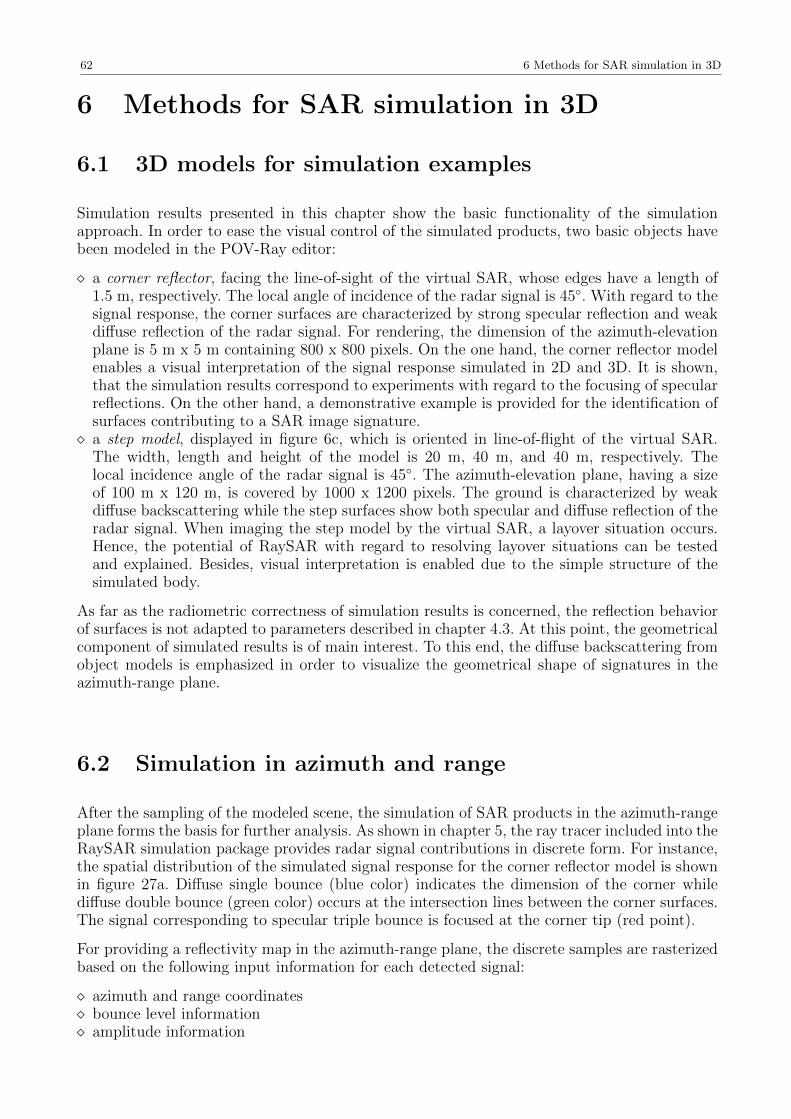
62 6 Methods for SAR simulation in 3D
6 Methods for SAR simulation in 3D
6.1 3D models for simulation examples
Simulation results presented in this chapter show the basic functionality of the simulationapproach. In order to ease the visual control of the simulated products, two basic objects havebeen modeled in the POV-Ray editor:
a corner reflector, facing the line-of-sight of the virtual SAR, whose edges have a length of1.5 m, respectively. The local angle of incidence of the radar signal is 45. With regard to thesignal response, the corner surfaces are characterized by strong specular reflection and weakdiffuse reflection of the radar signal. For rendering, the dimension of the azimuth-elevationplane is 5 m x 5 m containing 800 x 800 pixels. On the one hand, the corner reflector modelenables a visual interpretation of the signal response simulated in 2D and 3D. It is shown,that the simulation results correspond to experiments with regard to the focusing of specularreflections. On the other hand, a demonstrative example is provided for the identification ofsurfaces contributing to a SAR image signature. a step model, displayed in figure 6c, which is oriented in line-of-flight of the virtual SAR.
The width, length and height of the model is 20 m, 40 m, and 40 m, respectively. Thelocal incidence angle of the radar signal is 45. The azimuth-elevation plane, having a sizeof 100 m x 120 m, is covered by 1000 x 1200 pixels. The ground is characterized by weakdiffuse backscattering while the step surfaces show both specular and diffuse reflection of theradar signal. When imaging the step model by the virtual SAR, a layover situation occurs.Hence, the potential of RaySAR with regard to resolving layover situations can be testedand explained. Besides, visual interpretation is enabled due to the simple structure of thesimulated body.
As far as the radiometric correctness of simulation results is concerned, the reflection behaviorof surfaces is not adapted to parameters described in chapter 4.3. At this point, the geometricalcomponent of simulated results is of main interest. To this end, the diffuse backscattering fromobject models is emphasized in order to visualize the geometrical shape of signatures in theazimuth-range plane.
6.2 Simulation in azimuth and range
After the sampling of the modeled scene, the simulation of SAR products in the azimuth-rangeplane forms the basis for further analysis. As shown in chapter 5, the ray tracer included into theRaySAR simulation package provides radar signal contributions in discrete form. For instance,the spatial distribution of the simulated signal response for the corner reflector model is shownin figure 27a. Diffuse single bounce (blue color) indicates the dimension of the corner whilediffuse double bounce (green color) occurs at the intersection lines between the corner surfaces.The signal corresponding to specular triple bounce is focused at the corner tip (red point).
For providing a reflectivity map in the azimuth-range plane, the discrete samples are rasterizedbased on the following input information for each detected signal:
azimuth and range coordinates bounce level information amplitude information
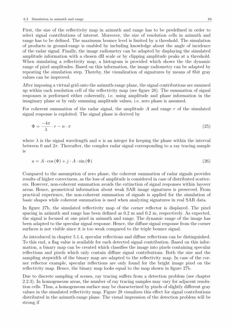
6.2 Simulation in azimuth and range 63
First, the size of the reflectivity map in azimuth and range has to be predefined in order toselect signal contributions of interest. Moreover, the size of resolution cells in azimuth andrange has to be defined. The maximum bounce level is limited by a threshold. The simulationof products in ground-range is enabled by including knowledge about the angle of incidenceof the radar signal. Finally, the image radiometry can be adapted by displaying the simulatedamplitude information with a chosen dB scale or by clipping amplitude peaks at a threshold.When simulating a reflectivity map, a histogram is provided which shows the the dynamicrange of pixel amplitudes. Based on this information, the image radiometry can be adapted byrepeating the simulation step. Thereby, the visualization of signatures by means of 8bit grayvalues can be improved.
After imposing a virtual grid onto the azimuth-range plane, the signal contributions are summedup within each resolution cell of the reflectivity map (see figure 28). The summation of signalresponses is performed either coherently, i.e. using amplitude and phase information in theimaginary plane or by only summing amplitude values, i.e. zero phase is assumed.
For coherent summation of the radar signal, the amplitude A and range r of the simulatedsignal response is exploited. The signal phase is derived by
Φ =−4π
λ· r − n · π (25)
where λ is the signal wavelength and n is an integer for keeping the phase within the intervalbetween 0 and 2π. Thereafter, the complex radar signal corresponding to a ray tracing sampleis
u = A · cos (Φ) + j · A · sin (Φ) (26)
Compared to the assumption of zero phase, the coherent summation of radar signals providesresults of higher correctness, as the loss of amplitude is considered in case of distributed scatter-ers. However, non-coherent summation avoids the extinction of signal responses within layoverareas. Hence, geometrical information about weak SAR image signatures is preserved. Frompractical experience, the non-coherent summation of signals is applied for the simulation ofbasic shapes while coherent summation is used when analyzing signatures in real SAR data.
In figure 27b, the simulated reflectivity map of the corner reflector is displayed. The pixelspacing in azimuth and range has been defined as 0.2 m and 0.2 m, respectively. As expected,the signal is focused at one pixel in azimuth and range. The dynamic range of the image hasbeen adapted to the specular signal response. Hence, the diffuse signal response from the cornersurfaces is not visible since it is too weak compared to the triple bounce signal.
As introduced in chapter 5.1.4, specular reflections and diffuse reflections can be distinguished.To this end, a flag value is available for each detected signal contribution. Based on this infor-mation, a binary map can be created which classifies the image into pixels containing specularreflections and pixels which only contain diffuse signal contributions. Both the size and thesampling stepwidth of the binary map are adapted to the reflectivity map. In case of the cor-ner reflector example, specular reflections are only found for the bright image pixel on thereflectivity map. Hence, the binary map looks equal to the map shown in figure 27b.
Due to discrete sampling of scenes, ray tracing suffers from a detection problem (see chapter2.2.3). In homogeneous areas, the number of ray tracing samples may vary for adjacent resolu-tion cells. Thus, a homogeneous surface may be characterized by pixels of slightly different grayvalues in the simulated reflectivity map. Figure 28 visualizes this effect for signal contributionsdistributed in the azimuth-range plane. The visual impression of the detection problem will bestrong if
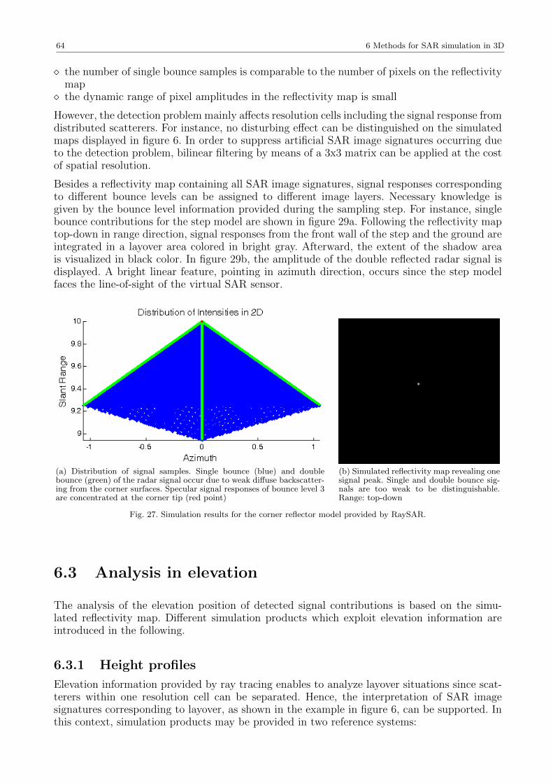
64 6 Methods for SAR simulation in 3D
the number of single bounce samples is comparable to the number of pixels on the reflectivitymap the dynamic range of pixel amplitudes in the reflectivity map is small
However, the detection problem mainly affects resolution cells including the signal response fromdistributed scatterers. For instance, no disturbing effect can be distinguished on the simulatedmaps displayed in figure 6. In order to suppress artificial SAR image signatures occurring dueto the detection problem, bilinear filtering by means of a 3x3 matrix can be applied at the costof spatial resolution.
Besides a reflectivity map containing all SAR image signatures, signal responses correspondingto different bounce levels can be assigned to different image layers. Necessary knowledge isgiven by the bounce level information provided during the sampling step. For instance, singlebounce contributions for the step model are shown in figure 29a. Following the reflectivity maptop-down in range direction, signal responses from the front wall of the step and the ground areintegrated in a layover area colored in bright gray. Afterward, the extent of the shadow areais visualized in black color. In figure 29b, the amplitude of the double reflected radar signal isdisplayed. A bright linear feature, pointing in azimuth direction, occurs since the step modelfaces the line-of-sight of the virtual SAR sensor.
(a) Distribution of signal samples. Single bounce (blue) and doublebounce (green) of the radar signal occur due to weak diffuse backscatter-ing from the corner surfaces. Specular signal responses of bounce level 3are concentrated at the corner tip (red point)
(b) Simulated reflectivity map revealing onesignal peak. Single and double bounce sig-nals are too weak to be distinguishable.Range: top-down
Fig. 27. Simulation results for the corner reflector model provided by RaySAR.
6.3 Analysis in elevation
The analysis of the elevation position of detected signal contributions is based on the simu-lated reflectivity map. Different simulation products which exploit elevation information areintroduced in the following.
6.3.1 Height profiles
Elevation information provided by ray tracing enables to analyze layover situations since scat-terers within one resolution cell can be separated. Hence, the interpretation of SAR imagesignatures corresponding to layover, as shown in the example in figure 6, can be supported. Inthis context, simulation products may be provided in two reference systems:
6.3 Analysis in elevation 65
Fig. 28. Rasterization of ray tracing samples: signal contributions are summed up within each resolution cell in theazimuth-range plane. The summation is performed either coherently, i.e. using amplitude and phase information, or onlyusing amplitude information.
(a) Single Bounce (b) Double Bounce (c) Pixel of interest (d) Defined profiles
Fig. 29. Step model: separation of bounces and definition of elevation profiles for a pixel of interest. Profiles #1 and #2are defined for displaying elevation information in range and azimuth. Profile #3 is defined perpendicularly to the imageplane and enables to display the distribution of signal responses in cross-range direction. Azimuth: left-right. Range:top-down.
(1) elevation: coordinates in cross-range direction which are directly provided by the samplingstep. The elevation coordinate of 0 m corresponds to the center of the sensor plane definedfor the rendering process.
(2) height over ground : height with respect to a reference point on the ground surroundingthe simulated object. The transformation of the elevation coordinates to the height-over-ground system is enabled by the known angle of incidence of the radar signal and theassumption of a flat ground surrounding the building.
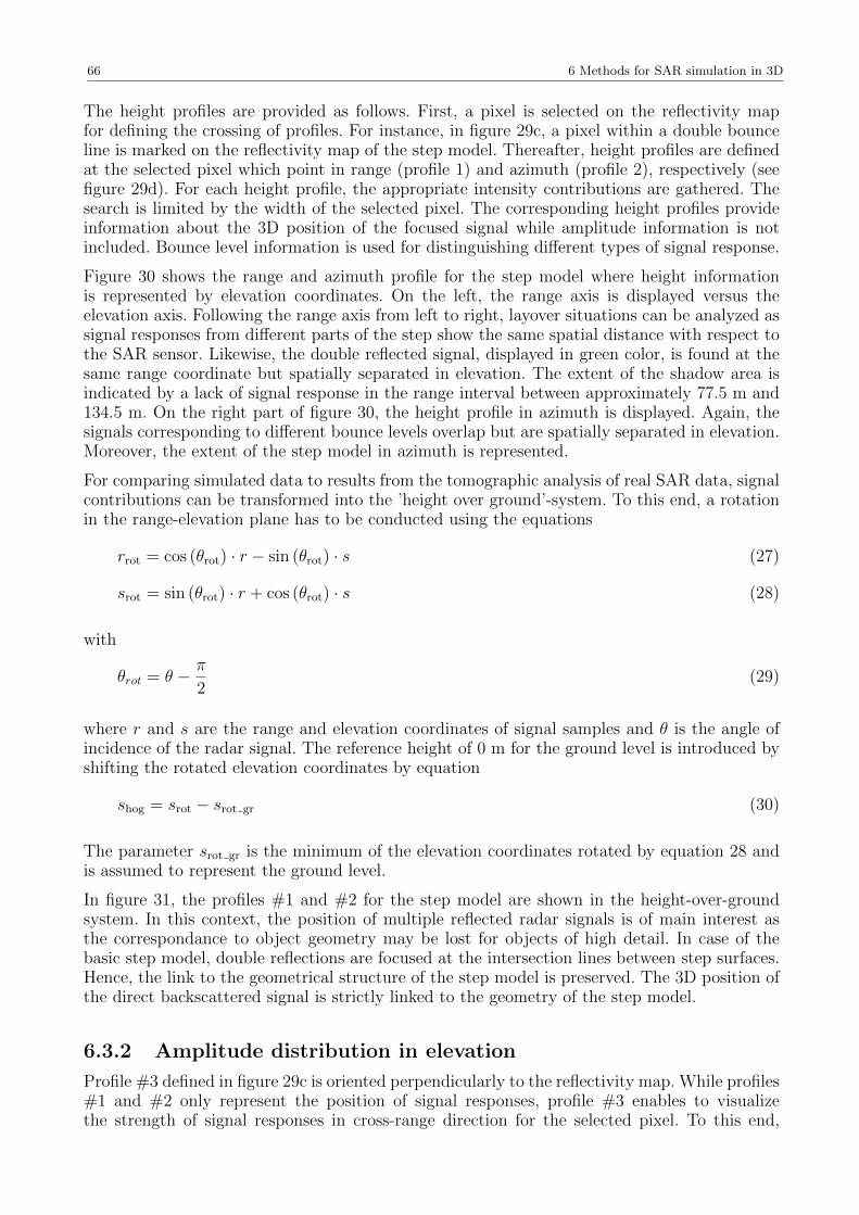
66 6 Methods for SAR simulation in 3D
The height profiles are provided as follows. First, a pixel is selected on the reflectivity mapfor defining the crossing of profiles. For instance, in figure 29c, a pixel within a double bounceline is marked on the reflectivity map of the step model. Thereafter, height profiles are definedat the selected pixel which point in range (profile 1) and azimuth (profile 2), respectively (seefigure 29d). For each height profile, the appropriate intensity contributions are gathered. Thesearch is limited by the width of the selected pixel. The corresponding height profiles provideinformation about the 3D position of the focused signal while amplitude information is notincluded. Bounce level information is used for distinguishing different types of signal response.
Figure 30 shows the range and azimuth profile for the step model where height informationis represented by elevation coordinates. On the left, the range axis is displayed versus theelevation axis. Following the range axis from left to right, layover situations can be analyzed assignal responses from different parts of the step show the same spatial distance with respect tothe SAR sensor. Likewise, the double reflected signal, displayed in green color, is found at thesame range coordinate but spatially separated in elevation. The extent of the shadow area isindicated by a lack of signal response in the range interval between approximately 77.5 m and134.5 m. On the right part of figure 30, the height profile in azimuth is displayed. Again, thesignals corresponding to different bounce levels overlap but are spatially separated in elevation.Moreover, the extent of the step model in azimuth is represented.
For comparing simulated data to results from the tomographic analysis of real SAR data, signalcontributions can be transformed into the ’height over ground’-system. To this end, a rotationin the range-elevation plane has to be conducted using the equations
rrot = cos (θrot) · r − sin (θrot) · s (27)
srot = sin (θrot) · r + cos (θrot) · s (28)
with
θrot = θ − π
2(29)
where r and s are the range and elevation coordinates of signal samples and θ is the angle ofincidence of the radar signal. The reference height of 0 m for the ground level is introduced byshifting the rotated elevation coordinates by equation
shog = srot − srot gr (30)
The parameter srot gr is the minimum of the elevation coordinates rotated by equation 28 andis assumed to represent the ground level.
In figure 31, the profiles #1 and #2 for the step model are shown in the height-over-groundsystem. In this context, the position of multiple reflected radar signals is of main interest asthe correspondance to object geometry may be lost for objects of high detail. In case of thebasic step model, double reflections are focused at the intersection lines between step surfaces.Hence, the link to the geometrical structure of the step model is preserved. The 3D position ofthe direct backscattered signal is strictly linked to the geometry of the step model.
6.3.2 Amplitude distribution in elevation
Profile #3 defined in figure 29c is oriented perpendicularly to the reflectivity map. While profiles#1 and #2 only represent the position of signal responses, profile #3 enables to visualizethe strength of signal responses in cross-range direction for the selected pixel. To this end,
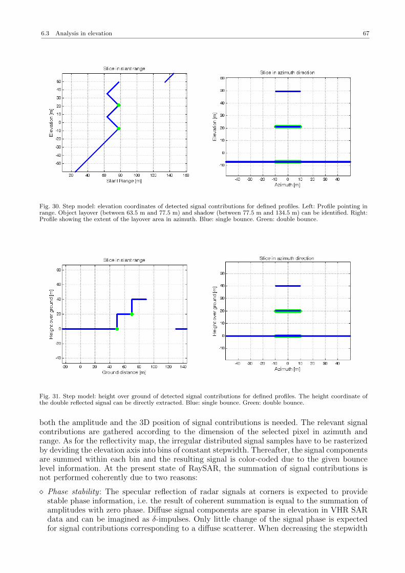
6.3 Analysis in elevation 67
Fig. 30. Step model: elevation coordinates of detected signal contributions for defined profiles. Left: Profile pointing inrange. Object layover (between 63.5 m and 77.5 m) and shadow (between 77.5 m and 134.5 m) can be identified. Right:Profile showing the extent of the layover area in azimuth. Blue: single bounce. Green: double bounce.
Fig. 31. Step model: height over ground of detected signal contributions for defined profiles. The height coordinate ofthe double reflected signal can be directly extracted. Blue: single bounce. Green: double bounce.
both the amplitude and the 3D position of signal contributions is needed. The relevant signalcontributions are gathered according to the dimension of the selected pixel in azimuth andrange. As for the reflectivity map, the irregular distributed signal samples have to be rasterizedby deviding the elevation axis into bins of constant stepwidth. Thereafter, the signal componentsare summed within each bin and the resulting signal is color-coded due to the given bouncelevel information. At the present state of RaySAR, the summation of signal contributions isnot performed coherently due to two reasons:
Phase stability : The specular reflection of radar signals at corners is expected to providestable phase information, i.e. the result of coherent summation is equal to the summation ofamplitudes with zero phase. Diffuse signal components are sparse in elevation in VHR SARdata and can be imagined as δ-impulses. Only little change of the signal phase is expectedfor signal contributions corresponding to a diffuse scatterer. When decreasing the stepwidth
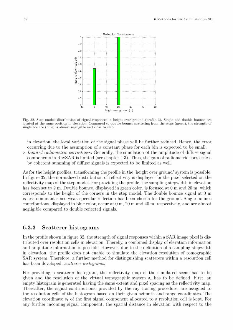
68 6 Methods for SAR simulation in 3D
Fig. 32. Step model: distribution of signal responses in height over ground (profile 3). Single and double bounce arelocated at the same position in elevation. Compared to double bounce scattering from the steps (green), the strength ofsingle bounce (blue) is almost negligible and close to zero.
in elevation, the local variation of the signal phase will be further reduced. Hence, the erroroccurring due to the assumption of a constant phase for each bin is expected to be small. Limited radiometric correctness : Generally, the simulation of the amplitude of diffuse signal
components in RaySAR is limited (see chapter 4.3). Thus, the gain of radiometric correctnessby coherent summing of diffuse signals is expected to be limited as well.
As for the height profiles, transforming the profile in the ’height over ground’ system is possible.In figure 32, the normalized distribution of reflectivity is displayed for the pixel selected on thereflectivity map of the step model. For providing the profile, the sampling stepwidth in elevationhas been set to 2 m. Double bounce, displayed in green color, is focused at 0 m and 20 m, whichcorresponds to the height of the corners in the step model. The double bounce signal at 0 mis less dominant since weak specular reflection has been chosen for the ground. Single bouncecontributions, displayed in blue color, occur at 0 m, 20 m and 40 m, respectively, and are almostnegligible compared to double reflected signals.
6.3.3 Scatterer histograms
In the profile shown in figure 32, the strength of signal responses within a SAR image pixel is dis-tributed over resolution cells in elevation. Thereby, a combined display of elevation informationand amplitude information is possible. However, due to the definition of a sampling stepwidthin elevation, the profile does not enable to simulate the elevation resolution of tomographicSAR system. Therefore, a further method for distinguishing scatterers within a resolution cellhas been developed: scatterer histograms.
For providing a scatterer histogram, the reflectivity map of the simulated scene has to begiven and the resolution of the virtual tomographic system δs has to be defined. First, anempty histogram is generated having the same extent and pixel spacing as the reflectivity map.Thereafter, the signal contributions, provided by the ray tracing procedure, are assigned tothe resolution cells of the histogram based on their given azimuth and range coordinates. Theelevation coordinate s1 of the first signal component allocated to a resolution cell is kept. Forany further incoming signal component, the spatial distance in elevation with respect to the
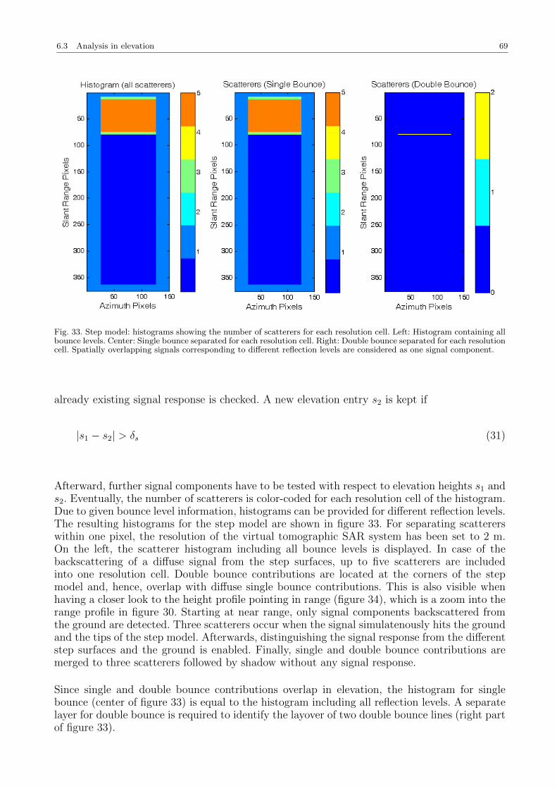
6.3 Analysis in elevation 69
Fig. 33. Step model: histograms showing the number of scatterers for each resolution cell. Left: Histogram containing allbounce levels. Center: Single bounce separated for each resolution cell. Right: Double bounce separated for each resolutioncell. Spatially overlapping signals corresponding to different reflection levels are considered as one signal component.
already existing signal response is checked. A new elevation entry s2 is kept if
|s1 − s2| > δs (31)
Afterward, further signal components have to be tested with respect to elevation heights s1 ands2. Eventually, the number of scatterers is color-coded for each resolution cell of the histogram.Due to given bounce level information, histograms can be provided for different reflection levels.The resulting histograms for the step model are shown in figure 33. For separating scattererswithin one pixel, the resolution of the virtual tomographic SAR system has been set to 2 m.On the left, the scatterer histogram including all bounce levels is displayed. In case of thebackscattering of a diffuse signal from the step surfaces, up to five scatterers are includedinto one resolution cell. Double bounce contributions are located at the corners of the stepmodel and, hence, overlap with diffuse single bounce contributions. This is also visible whenhaving a closer look to the height profile pointing in range (figure 34), which is a zoom into therange profile in figure 30. Starting at near range, only signal components backscattered fromthe ground are detected. Three scatterers occur when the signal simulatenously hits the groundand the tips of the step model. Afterwards, distinguishing the signal response from the differentstep surfaces and the ground is enabled. Finally, single and double bounce contributions aremerged to three scatterers followed by shadow without any signal response.
Since single and double bounce contributions overlap in elevation, the histogram for singlebounce (center of figure 33) is equal to the histogram including all reflection levels. A separatelayer for double bounce is required to identify the layover of two double bounce lines (right partof figure 33).
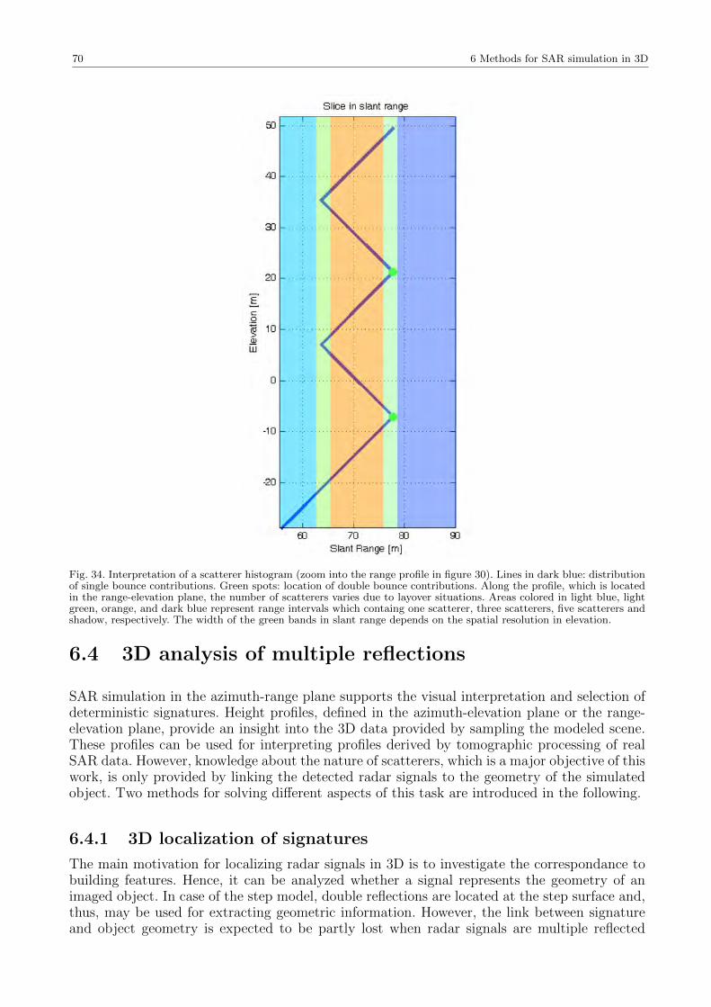
70 6 Methods for SAR simulation in 3D
Fig. 34. Interpretation of a scatterer histogram (zoom into the range profile in figure 30). Lines in dark blue: distributionof single bounce contributions. Green spots: location of double bounce contributions. Along the profile, which is locatedin the range-elevation plane, the number of scatterers varies due to layover situations. Areas colored in light blue, lightgreen, orange, and dark blue represent range intervals which containg one scatterer, three scatterers, five scatterers andshadow, respectively. The width of the green bands in slant range depends on the spatial resolution in elevation.
6.4 3D analysis of multiple reflections
SAR simulation in the azimuth-range plane supports the visual interpretation and selection ofdeterministic signatures. Height profiles, defined in the azimuth-elevation plane or the range-elevation plane, provide an insight into the 3D data provided by sampling the modeled scene.These profiles can be used for interpreting profiles derived by tomographic processing of realSAR data. However, knowledge about the nature of scatterers, which is a major objective of thiswork, is only provided by linking the detected radar signals to the geometry of the simulatedobject. Two methods for solving different aspects of this task are introduced in the following.
6.4.1 3D localization of signatures
The main motivation for localizing radar signals in 3D is to investigate the correspondance tobuilding features. Hence, it can be analyzed whether a signal represents the geometry of animaged object. In case of the step model, double reflections are located at the step surface and,thus, may be used for extracting geometric information. However, the link between signatureand object geometry is expected to be partly lost when radar signals are multiple reflected
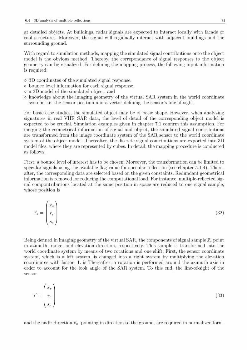
6.4 3D analysis of multiple reflections 71
at detailed objects. At buildings, radar signals are expected to interact locally with facade orroof structures. Moreover, the signal will regionally interact with adjacent buildings and thesurrounding ground.
With regard to simulation methods, mapping the simulated signal contributions onto the objectmodel is the obvious method. Thereby, the correpondance of signal responses to the objectgeometry can be visualized. For defining the mapping process, the following input informationis required:
3D coordinates of the simulated signal response, bounce level information for each signal response, a 3D model of the simulated object, and knowledge about the imaging geometry of the virtual SAR system in the world coordinate
system, i.e. the sensor position and a vector defining the sensor’s line-of-sight.
For basic case studies, the simulated object may be of basic shape. However, when analyzingsignatures in real VHR SAR data, the level of detail of the corresponding object model isexpected to be crucial. Simulation examples given in chapter 7.1 confirm this assumption. Formerging the geometrical information of signal and object, the simulated signal contributionsare transformed from the image coordinate system of the SAR sensor to the world coordinatesystem of the object model. Thereafter, the discrete signal contributions are exported into 3Dmodel files, where they are represented by cubes. In detail, the mapping procedure is conductedas follows.
First, a bounce level of interest has to be chosen. Moreover, the transformation can be limited tospecular signals using the available flag value for specular reflection (see chapter 5.1.4). There-after, the corresponding data are selected based on the given constaints. Redundant geometricalinformation is removed for reducing the computational load. For instance, multiple-reflected sig-nal compontributions located at the same position in space are reduced to one signal sample,whose position is
~xs =
xs
rs
ss
(32)
Being defined in imaging geometry of the virtual SAR, the components of signal sample ~xs pointin azimuth, range, and elevation direction, respectively. This sample is transformed into theworld coordinate system by means of two rotations and one shift. First, the sensor coordinatesystem, which is a left system, is changed into a right system by multiplying the elevationcoordinates with factor -1. is Thereafter, a rotation is performed around the azimuth axis inorder to account for the look angle of the SAR system. To this end, the line-of-sight of thesensor
~r =
xr
rr
sr
(33)
and the nadir direction ~vn, pointing in direction to the ground, are required in normalized form.
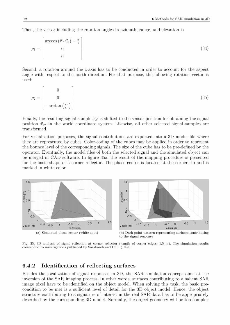
72 6 Methods for SAR simulation in 3D
Then, the vector including the rotation angles in azimuth, range, and elevation is
ρ1 =
arccos (~r · ~vn)− π
2
0
0
(34)
Second, a rotation around the z-axis has to be conducted in order to account for the aspectangle with respect to the north direction. For that purpose, the following rotation vector isused:
ρ2 =
0
0
−arctan(xrrr
) (35)
Finally, the resulting signal sample ~xs′ is shifted to the sensor position for obtaining the signalposition ~xs′′ in the world coordinate system. Likewise, all other selected signal samples aretransformed.
For visualization purposes, the signal contributions are exported into a 3D model file wherethey are represented by cubes. Color-coding of the cubes may be applied in order to representthe bounce level of the corresponding signals. The size of the cube has to be pre-defined by theoperator. Eventually, the model files of both the selected signal and the simulated object canbe merged in CAD software. In figure 35a, the result of the mapping procedure is presentedfor the basic shape of a corner reflector. The phase center is located at the corner tip and ismarked in white color.
(a) Simulated phase center (white spot) (b) Dark point pattern representing surfaces contributingto the signal response
Fig. 35. 3D analysis of signal reflection at corner reflector (length of corner edges: 1.5 m). The simulation resultscorrespond to investigations published by Sarabandi and Chiu (1996).
6.4.2 Identification of reflecting surfaces
Besides the localization of signal responses in 3D, the SAR simulation concept aims at theinversion of the SAR imaging process. In other words, surfaces contributing to a salient SARimage pixel have to be identified on the object model. When solving this task, the basic pre-condition to be met is a sufficient level of detail for the 3D object model. Hence, the objectstructure contributing to a signature of interest in the real SAR data has to be appropriatelydescribed by the corresponding 3D model. Normally, the object geometry will be too complex
6.4 3D analysis of multiple reflections 73
and, hence, will not be perfectly met by the 3D model. However, the level of generalizationshould be low enough. Then, RaySAR enables to approximate the inversion of the imagingprocess of a SAR system.
As ray tracing is performed by means of samples, no surfaces are detected on reflecting objects.Instead, the distribution of intersection points can be mapped onto the object model. Thereby,the interaction of signals with scene objects is indicated. The proceeding of the mapping pro-cedure is introduced in the following.
As explained in chapter 5.1.1, the coordinates Xi, Yi, and Zi of each intersection point can bestored optionally during the sampling step. The position of the intersection points is definedin the world coordinate system of the object model. Thus, each detected signal is assigned toan intersection point. The necessary link between the azimuth-range plane and the 3D objectgeometry is provided by selecting a pixel of interest on the simulated reflectivity map (seechapter 6.2). The size of the selected pixel limits the search for signal contributions and, hence,also limits the search for intersection points. Redundant geometrical information is locallyremoved, i.e. nearby intersection points corresponding to the same bounce level are reduced toone sample. When being exported to a 3D model file, the intersection points are represented bycubes whose size has to be predefined. The area of redundancy for intersection points is equalto the cube size. Hence, no cubes of the same bounce level will overlap in the 3D model file.
In case of single bounce of a radar signal, the coordinate of the corresponding intersection pointcan be directly extracted from the signal vector (see equation 20). In case of higher reflectionlevels, intersection points of lower reflection levels have to be considered as well. For instance,a triple bounce component may be given in the signal matrix by
Ss =
. . . . . . . . .
xs1 rs1 ss1 As1 1 fs1 Xi1 Yi1 Zi1
xs2 rs2 ss2 As2 2 fs2 Xi2 Yi2 Zi2
xs3 rs3 ss3 As3 3 fs3 Xi3 Yi3 Zi3
. . . . . . . . .
(36)
where the fifth column contains the bounce level information, i.e. numbers from 1 to 3. Whenanalyzing the triple bounce effect, the selection of a SAR image pixel will lead to the azimuthand range coordinates xs3 and rs3. These coordinates are directly linked to the intersectionpoint located at Xi3, Yi3, and Zi3. At this point, the radar signal was reflected for the first timein the scene, i.e. the intersection point for the first bounce is found. Since ray tracing followsone ray after another one, the corresponding signal response is ordered with increasing bouncelevel (see signal matrix in equation 36). Hence, starting at the current row in signal matrix Ss,the intersection points describing the second and third bounce can be found in the two rowsabove. In order to enable the identification of scatterers, intersection points corresponding to asignal reflection have to be stored even if no signal is detected. For the example at hand, thefirst and second row of matrix Ss always have to exist to fully describe the path of the reflectedsignal. For SAR simulation without the identification of scatterers, these rows are not stored ifthe amplitude values As1 and As2 are zero.
In figure 35b, the surfaces contributing to the triple bounce signal of the corner reflector modelare marked by a dark pattern of points. As expected, the effective reflecting surface, contributingto the specular highlight in figure 27b, is smaller than the corner surface and forms a pentagonalshape. In reality, the illuminated surface of the corner reflector will slightly change along thesynthetic aperture and, thus, will be slightly differerent to the simulated result. However, thedifference will be small due to the small angular range of the spaceborne SAR system.
74 6 Methods for SAR simulation in 3D
The density of intersection points on the reflecting surfaces enables to visually control thesampling of the corner reflector. Eventually, color-coding may be applied for displaying differ-ent bounce levels. In the corner reflector example, color-coding is dissabled since only triplereflection of the radar signal occurs.
6.5 Discussion
Simulated reflectivity maps only enable the visual comparison to real SAR data. Visual in-terpretation is hardly supported as signatures corresponding to different bounce levels maybe confused. Hence, reflectivity maps can only considered as a basic product to be used fortriggering further analysis of SAR image signatures.
When assigning different bounce levels to separate layers, however, the focus can be put onsignatures of interest. For instance, linear features corresponding to foreshortening can then bevisually distinguished from double bounce lines. With regard to the application to real SARdata, layers containing different bounce levels can provide specific geometrical informationabout objects, e.g.:
Layer for single bounce: provides the geometrical shape of objects in the azimuth-range planeand enables to identify layover situations. To this end, the emphasis of a signal response fromthe object of interest is reasonable. Moreover, the extent of shadow can be visualized. Layer for double bounce: provides geometrical information about the location of diffuse or
specular double reflections. Double reflections of signals can occur at one single object, e.g.at protrusions on a building facades, or due to signal interaction with adjacent objects, e.g.a building wall and the surrounding ground. Layer for triple bounce: provides the position of signal responses corresponding to diffuse
or specular triple reflections. Triple bounce of specular kind is expected to cause dominantpoint signatures in SAR data. Moreover, point signatures may be helpful for coregisteringsimulated and real SAR data as the power peak of a trihedral is always located within oneresolution cell.
When creating the image layers, the signal contributions are separated based on bounce levelinformation. Accordingly, diffuse and specular reflections of the same bounce level are inte-grated into one image layer. However, distinguishing between specular and non-specular signalresponses should be enabled for two purposes. First, specular reflections may be underestimatedby RaySAR due to inappropriate settings for the reflection models or due to local undersamplingof object features. The identification of specular reflections may help to compensate for theselimitations as specular signal responses are marked. Moreover, the focus should be on specularsignals when exploiting the simulated data for analyzing real SAR data. The reason is that forspecular reflections the geometrical correctness of azimuth focusing is higher than for diffusereflections (see chapter 5.1.2). For distinguishing specular reflections, binary maps are createdfor each bounce level where specular reflections are marked. Hence, pixels containing specularsignal responses from e.g. direct backscattering, dihedrals or trihedrals can be identified in thesimulated data.
Height profiles can be extracted for each pixel on the reflectivity map. By analyzing the distribu-tion of radar signals in the elevation-range plane, layover situations can be resolved. Moreover,the elevation of the simulated radar signal can be displayed with respect to a reference point onthe ground. Then, the height of multiple reflected signals can be analyzed on simulated objects.The simulated profiles can be compared to height profiles from SAR tomography, which arecommonly visualized in height with respect to a reference point.
For each pixel of the reflectivity map, the amplitude distribution can be simulated. To thisend, the sampling stepwidth in elevation has to be defined. The radiometric correctness of
6.5 Discussion 75
simulated amplitudes is moderate due to the simplified reflection models of RaySAR. However,the position of the simulated amplitudes can be compared to signal peaks extracted fromreflectivity functions provided by SAR tomography. Comparable to the azimuth domain, thebest result is expected for specular reflected signals whose signal peak is located within oneresolution cell in elevation. Nonetheless, the spatial resolution of the tomographic SAR systemcan not be considered when simulating the amplitude distribution in elevation. Hence, as acomplementary tool, scatterer histograms enable to count the number of scatterers within eachresolution cell on the reflectivity map, given a spatial resolution in elevation. In this regard,the selection of relevant radar signals can be limited to a bounce level of interest. For instance,a histogram containing all bounce levels provides a general overview of layover effects in thesimulated scene. Separate histograms for multiple reflections enable to recover the layover ofdominant scatterers. Finally, simulated scatterer histograms may support SAR tomographybased on parametric models where the number of scatterers within a resolution cell has to beknown a-priori.
Height profiles in azimuth and range only provide an insight in the simulated 3D data. Thenature of scatterers has to be investigated in the world coordinate system of the object. To thisend, the simulated signals can be mapped into the model scene in order to merge the radarsignal and the object geometry in CAD software. Thereby, the detected signal can be locatedon the simulated object. The 3D distribution of simulated radar signals can be compared toresults provided by methods for localizing scatterers in real SAR data (see chapter 2.1.5).For identifying scatterers at objects, the surfaces contributing to an image signature can bemarked in the model scene. More specifically, salient signatures can be analyzed with regard totheir origin. Thus, methods focused on the exploitation of salient SAR image features can besupported, e.g. methods for object extraction/monitoring or Persistent Scatterer Interferometry(see chapters 2.1.4 and 2.1.5).
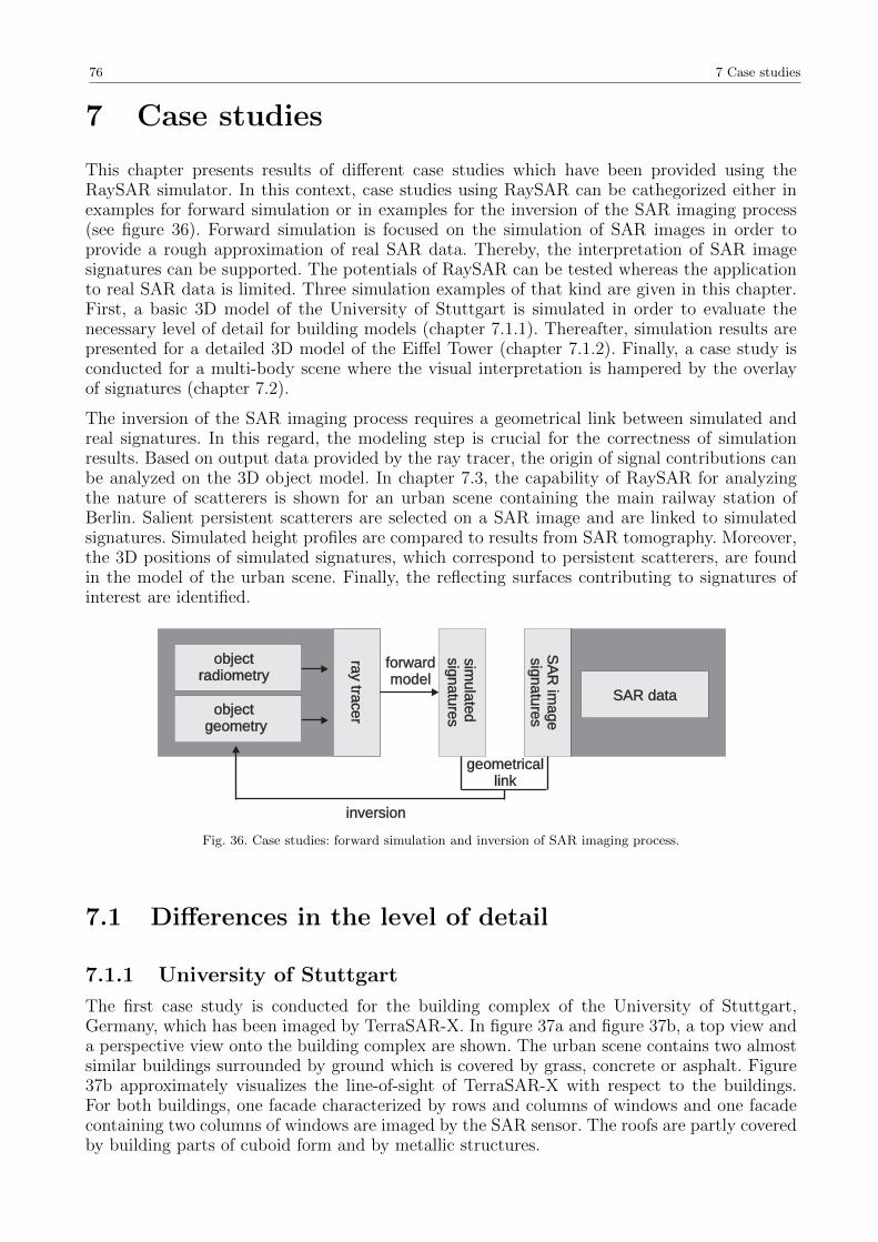
76 7 Case studies
7 Case studies
This chapter presents results of different case studies which have been provided using theRaySAR simulator. In this context, case studies using RaySAR can be cathegorized either inexamples for forward simulation or in examples for the inversion of the SAR imaging process(see figure 36). Forward simulation is focused on the simulation of SAR images in order toprovide a rough approximation of real SAR data. Thereby, the interpretation of SAR imagesignatures can be supported. The potentials of RaySAR can be tested whereas the applicationto real SAR data is limited. Three simulation examples of that kind are given in this chapter.First, a basic 3D model of the University of Stuttgart is simulated in order to evaluate thenecessary level of detail for building models (chapter 7.1.1). Thereafter, simulation results arepresented for a detailed 3D model of the Eiffel Tower (chapter 7.1.2). Finally, a case study isconducted for a multi-body scene where the visual interpretation is hampered by the overlayof signatures (chapter 7.2).
The inversion of the SAR imaging process requires a geometrical link between simulated andreal signatures. In this regard, the modeling step is crucial for the correctness of simulationresults. Based on output data provided by the ray tracer, the origin of signal contributions canbe analyzed on the 3D object model. In chapter 7.3, the capability of RaySAR for analyzingthe nature of scatterers is shown for an urban scene containing the main railway station ofBerlin. Salient persistent scatterers are selected on a SAR image and are linked to simulatedsignatures. Simulated height profiles are compared to results from SAR tomography. Moreover,the 3D positions of simulated signatures, which correspond to persistent scatterers, are foundin the model of the urban scene. Finally, the reflecting surfaces contributing to signatures ofinterest are identified.
sim
ula
ted
sig
natu
res
sim
ula
ted
sig
natu
res
SA
Rim
age
sig
natu
res
SA
Rim
age
sig
natu
res
SAR dataSAR data
forwardmodel
forwardmodel
inversion
geometricallink
geometricallink
objectgeometry
objectgeometry
objectradiometry
objectradiometry
ray
tracer
ray
tracer
Fig. 36. Case studies: forward simulation and inversion of SAR imaging process.
7.1 Differences in the level of detail
7.1.1 University of Stuttgart
The first case study is conducted for the building complex of the University of Stuttgart,Germany, which has been imaged by TerraSAR-X. In figure 37a and figure 37b, a top view anda perspective view onto the building complex are shown. The urban scene contains two almostsimilar buildings surrounded by ground which is covered by grass, concrete or asphalt. Figure37b approximately visualizes the line-of-sight of TerraSAR-X with respect to the buildings.For both buildings, one facade characterized by rows and columns of windows and one facadecontaining two columns of windows are imaged by the SAR sensor. The roofs are partly coveredby building parts of cuboid form and by metallic structures.
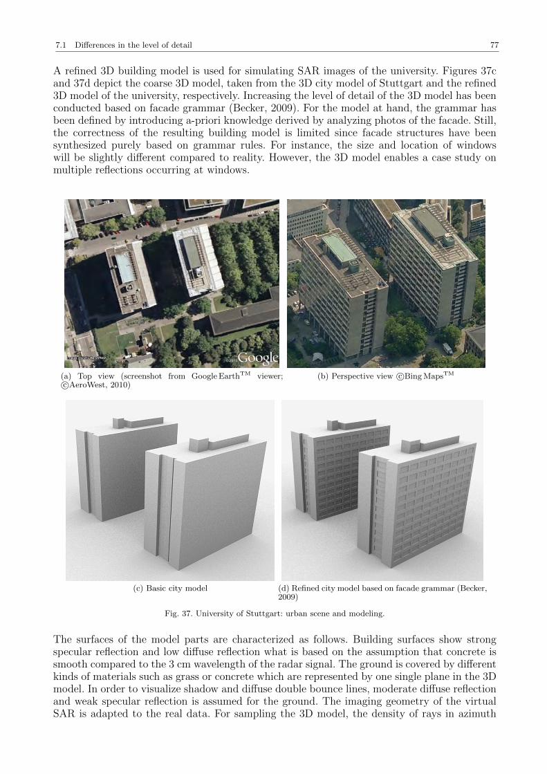
7.1 Differences in the level of detail 77
A refined 3D building model is used for simulating SAR images of the university. Figures 37cand 37d depict the coarse 3D model, taken from the 3D city model of Stuttgart and the refined3D model of the university, respectively. Increasing the level of detail of the 3D model has beenconducted based on facade grammar (Becker, 2009). For the model at hand, the grammar hasbeen defined by introducing a-priori knowledge derived by analyzing photos of the facade. Still,the correctness of the resulting building model is limited since facade structures have beensynthesized purely based on grammar rules. For instance, the size and location of windowswill be slightly different compared to reality. However, the 3D model enables a case study onmultiple reflections occurring at windows.
(a) Top view (screenshot from Google EarthTM viewer;c©AeroWest, 2010)
(b) Perspective view c©Bing MapsTM
(c) Basic city model (d) Refined city model based on facade grammar (Becker,2009)
Fig. 37. University of Stuttgart: urban scene and modeling.
The surfaces of the model parts are characterized as follows. Building surfaces show strongspecular reflection and low diffuse reflection what is based on the assumption that concrete issmooth compared to the 3 cm wavelength of the radar signal. The ground is covered by differentkinds of materials such as grass or concrete which are represented by one single plane in the 3Dmodel. In order to visualize shadow and diffuse double bounce lines, moderate diffuse reflectionand weak specular reflection is assumed for the ground. The imaging geometry of the virtualSAR is adapted to the real data. For sampling the 3D model, the density of rays in azimuth
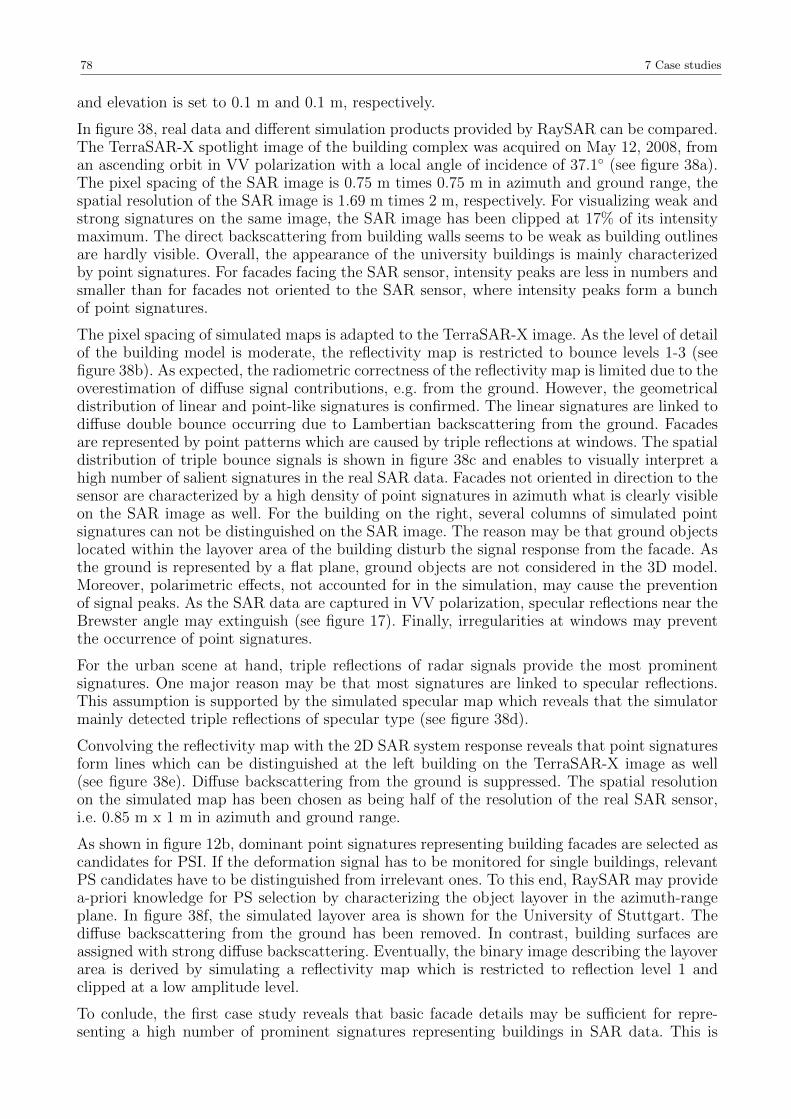
78 7 Case studies
and elevation is set to 0.1 m and 0.1 m, respectively.
In figure 38, real data and different simulation products provided by RaySAR can be compared.The TerraSAR-X spotlight image of the building complex was acquired on May 12, 2008, froman ascending orbit in VV polarization with a local angle of incidence of 37.1 (see figure 38a).The pixel spacing of the SAR image is 0.75 m times 0.75 m in azimuth and ground range, thespatial resolution of the SAR image is 1.69 m times 2 m, respectively. For visualizing weak andstrong signatures on the same image, the SAR image has been clipped at 17% of its intensitymaximum. The direct backscattering from building walls seems to be weak as building outlinesare hardly visible. Overall, the appearance of the university buildings is mainly characterizedby point signatures. For facades facing the SAR sensor, intensity peaks are less in numbers andsmaller than for facades not oriented to the SAR sensor, where intensity peaks form a bunchof point signatures.
The pixel spacing of simulated maps is adapted to the TerraSAR-X image. As the level of detailof the building model is moderate, the reflectivity map is restricted to bounce levels 1-3 (seefigure 38b). As expected, the radiometric correctness of the reflectivity map is limited due to theoverestimation of diffuse signal contributions, e.g. from the ground. However, the geometricaldistribution of linear and point-like signatures is confirmed. The linear signatures are linked todiffuse double bounce occurring due to Lambertian backscattering from the ground. Facadesare represented by point patterns which are caused by triple reflections at windows. The spatialdistribution of triple bounce signals is shown in figure 38c and enables to visually interpret ahigh number of salient signatures in the real SAR data. Facades not oriented in direction to thesensor are characterized by a high density of point signatures in azimuth what is clearly visibleon the SAR image as well. For the building on the right, several columns of simulated pointsignatures can not be distinguished on the SAR image. The reason may be that ground objectslocated within the layover area of the building disturb the signal response from the facade. Asthe ground is represented by a flat plane, ground objects are not considered in the 3D model.Moreover, polarimetric effects, not accounted for in the simulation, may cause the preventionof signal peaks. As the SAR data are captured in VV polarization, specular reflections near theBrewster angle may extinguish (see figure 17). Finally, irregularities at windows may preventthe occurrence of point signatures.
For the urban scene at hand, triple reflections of radar signals provide the most prominentsignatures. One major reason may be that most signatures are linked to specular reflections.This assumption is supported by the simulated specular map which reveals that the simulatormainly detected triple reflections of specular type (see figure 38d).
Convolving the reflectivity map with the 2D SAR system response reveals that point signaturesform lines which can be distinguished at the left building on the TerraSAR-X image as well(see figure 38e). Diffuse backscattering from the ground is suppressed. The spatial resolutionon the simulated map has been chosen as being half of the resolution of the real SAR sensor,i.e. 0.85 m x 1 m in azimuth and ground range.
As shown in figure 12b, dominant point signatures representing building facades are selected ascandidates for PSI. If the deformation signal has to be monitored for single buildings, relevantPS candidates have to be distinguished from irrelevant ones. To this end, RaySAR may providea-priori knowledge for PS selection by characterizing the object layover in the azimuth-rangeplane. In figure 38f, the simulated layover area is shown for the University of Stuttgart. Thediffuse backscattering from the ground has been removed. In contrast, building surfaces areassigned with strong diffuse backscattering. Eventually, the binary image describing the layoverarea is derived by simulating a reflectivity map which is restricted to reflection level 1 andclipped at a low amplitude level.
To conlude, the first case study reveals that basic facade details may be sufficient for repre-senting a high number of prominent signatures representing buildings in SAR data. This is
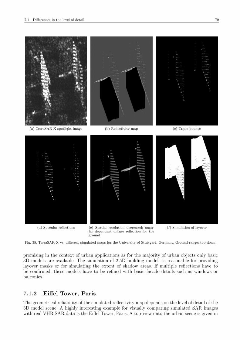
7.1 Differences in the level of detail 79
(a) TerraSAR-X spotlight image (b) Reflectivity map (c) Triple bounce
(d) Specular reflections (e) Spatial resolution decreased; angu-lar dependent diffuse reflection for theground
(f) Simulation of layover
Fig. 38. TerraSAR-X vs. different simulated maps for the University of Stuttgart, Germany. Ground-range: top-down.
promising in the context of urban applications as for the majority of urban objects only basic3D models are available. The simulation of 2.5D building models is reasonable for providinglayover masks or for simulating the extent of shadow areas. If multiple reflections have tobe confirmed, these models have to be refined with basic facade details such as windows orbalconies.
7.1.2 Eiffel Tower, Paris
The geometrical reliability of the simulated reflectivity map depends on the level of detail of the3D model scene. A highly interesting example for visually comparing simulated SAR imageswith real VHR SAR data is the Eiffel Tower, Paris. A top-view onto the urban scene is given in
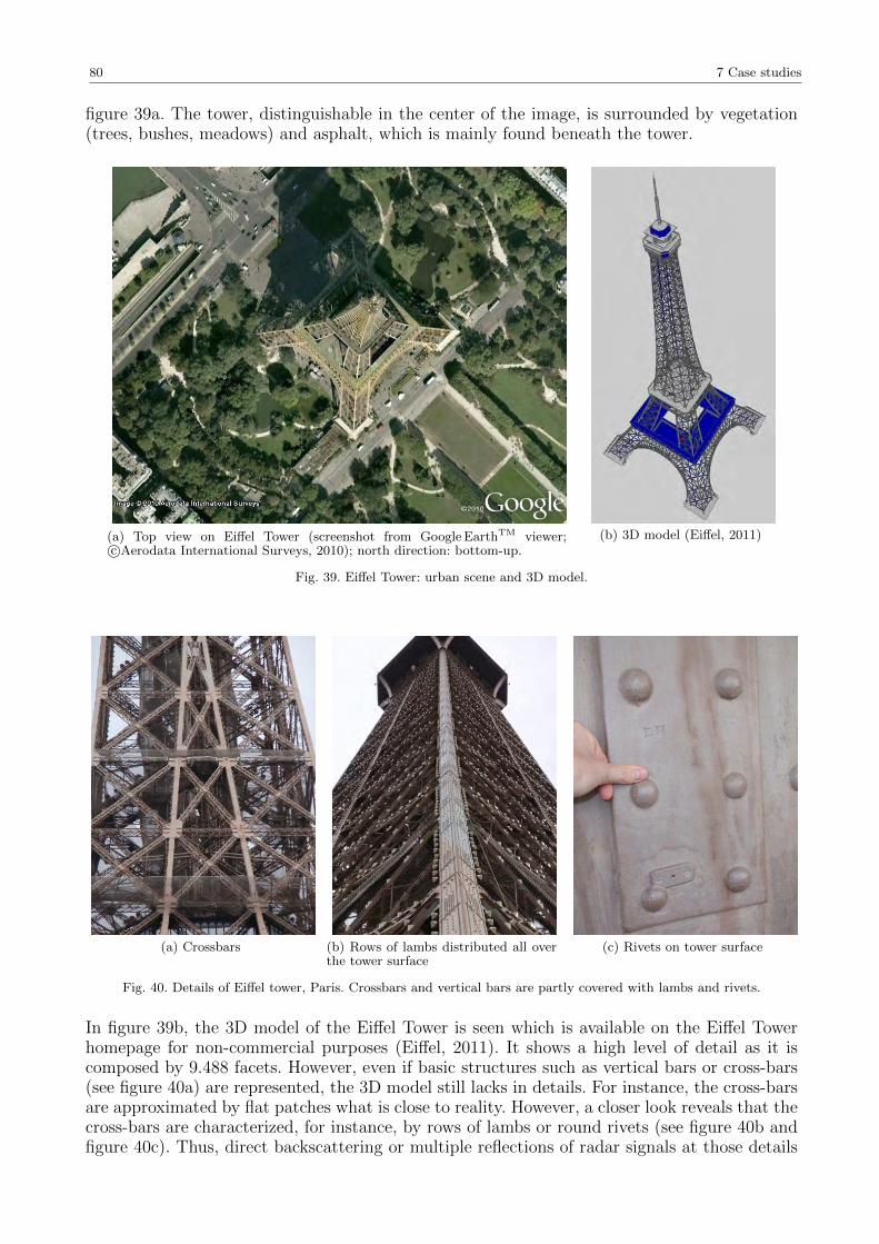
80 7 Case studies
figure 39a. The tower, distinguishable in the center of the image, is surrounded by vegetation(trees, bushes, meadows) and asphalt, which is mainly found beneath the tower.
(a) Top view on Eiffel Tower (screenshot from Google EarthTM viewer;c©Aerodata International Surveys, 2010); north direction: bottom-up.
(b) 3D model (Eiffel, 2011)
Fig. 39. Eiffel Tower: urban scene and 3D model.
(a) Crossbars (b) Rows of lambs distributed all overthe tower surface
(c) Rivets on tower surface
Fig. 40. Details of Eiffel tower, Paris. Crossbars and vertical bars are partly covered with lambs and rivets.
In figure 39b, the 3D model of the Eiffel Tower is seen which is available on the Eiffel Towerhomepage for non-commercial purposes (Eiffel, 2011). It shows a high level of detail as it iscomposed by 9.488 facets. However, even if basic structures such as vertical bars or cross-bars(see figure 40a) are represented, the 3D model still lacks in details. For instance, the cross-barsare approximated by flat patches what is close to reality. However, a closer look reveals that thecross-bars are characterized, for instance, by rows of lambs or round rivets (see figure 40b andfigure 40c). Thus, direct backscattering or multiple reflections of radar signals at those details
7.1 Differences in the level of detail 81
can not be confirmed by the simulator. Comparable to the university example in chapter 7.1.1,a compromise is necessary when defining the surface parameters of the tower.
Strong specular reflection and a high reflectivity factor are assigned to all tower surfaces. Inaddition, weak diffuse backscattering is added for roughly approximating local multiple reflec-tions at the crossbar details explained above. Since double bounce contributions caused by theinteraction between tower and ground are of interest, a flat plane is defined beneath the towermodel. It is characterized by low diffuse reflection in combination with strong reflectivity.
The imaging geometry of the virtual SAR, i.e. the angle of incidence and the heading angle,is adapted to the TerraSAR-X orbit. To this end, the tower is rotated and the local incidenceangle is set to 34.6. The number of rays in the azimuth-elevation plane is set to 1.000 inazimuth times 4.000, resulting in a sampling density of 0.1 m times 0.1 m. Sampling the 3Dmodel yields 4.13 million signal contributions.
For providing the reflectivity map, the pixel sampling is adapted to the sampling of the real SARdata, i.e. 0.43 m x 0.4 m in azimuth and ground range. The maximum number of reflections isset to 5 (figure 42a). In sum, the sampling of the 3D model and the creation of the reflectivitymap take 5 minutes and 14 seconds on a standard PC (2 GHz Dual Core, 4 GB RAM).
For comparison, a temporal average image has been created based on 6 TerraSAR-X spotlightdatasets. Hence, the appearance of the Eiffel Tower on the SAR image is characterized bydeterministic reflection effects as speckle is reduced (see figure 41a). Signal responses from thetower as well as from distributed scatterers on the ground are distinguishable. Due to a multi-looking factor of 2 in azimuth and range, the pixel spacing in the SAR image is 0.86 m x 0.8m in azimuth and ground range.
Figure 41 contains two simulated reflectivity maps. On the first one, signal contributions havebeen added non-coherently. For creating the second reflectivity map, the coherent summationof signal components has been considered (see figure 41c). On this map, the appearance of thetower components is more difficult to be distinguished as the layover of radar signal may causethe extinction of signal amplitudes. The coherently summed reflectivity map is more realisticthan the non-coherently summed one. However, the appearance of the Eiffel Tower can bebetter visually interpreted in figure 41b.
Compared to the real SAR image, many signatures are clearly visible on the reflectivity map aswell. The shortest distance with respect to the SAR sensor is obtained for the pinnacle (markedby letter A), followed by cross beam structures (B) in higher regions of the tower, two mainplattforms (C, D), three visible feet of the tower (E, F , G) and the shadow zone (H). Duringthe sampling step, a low amount of signal power penetrated the cross beam structures andcaused single bounce backscattering from the background of the tower. By contrast, this regionis almost completely shadowed in the SAR image. This might appear due to signal diffractionat tower crossbeams which is not considered in the simulation process. Moreover, the 3D modeldoes not contain any structures in the interior of the tower what is different to the real tower(see figure 39b and figure 40a).
In the 3D model used for SAR simulation, objects in the neighborhood of the tower are neglectedsince the ground is represented by a flat plane. Hence, the overlay of radar signals from towerand ground objects can not be confirmed by RaySAR but is clearly visible on the real SARimage. For instance, signatures C − G are overlaid with diffuse signals from vegetation orman-made structures in the neighborhood of the tower.
Double bounce signatures caused by signal interaction with the tower and the surroundingground show up at the bottom (I) and at both sides of the tower (J ,K). While signature (I) isalso apparent on the real SAR image, signatures (J) and (K) are not distinguishable. On theone hand, these signatures may dissappear because of objects covering the ground which avoidsignal backscattering to the sensor. Moreover, the diffuse reflection from the ground is defined
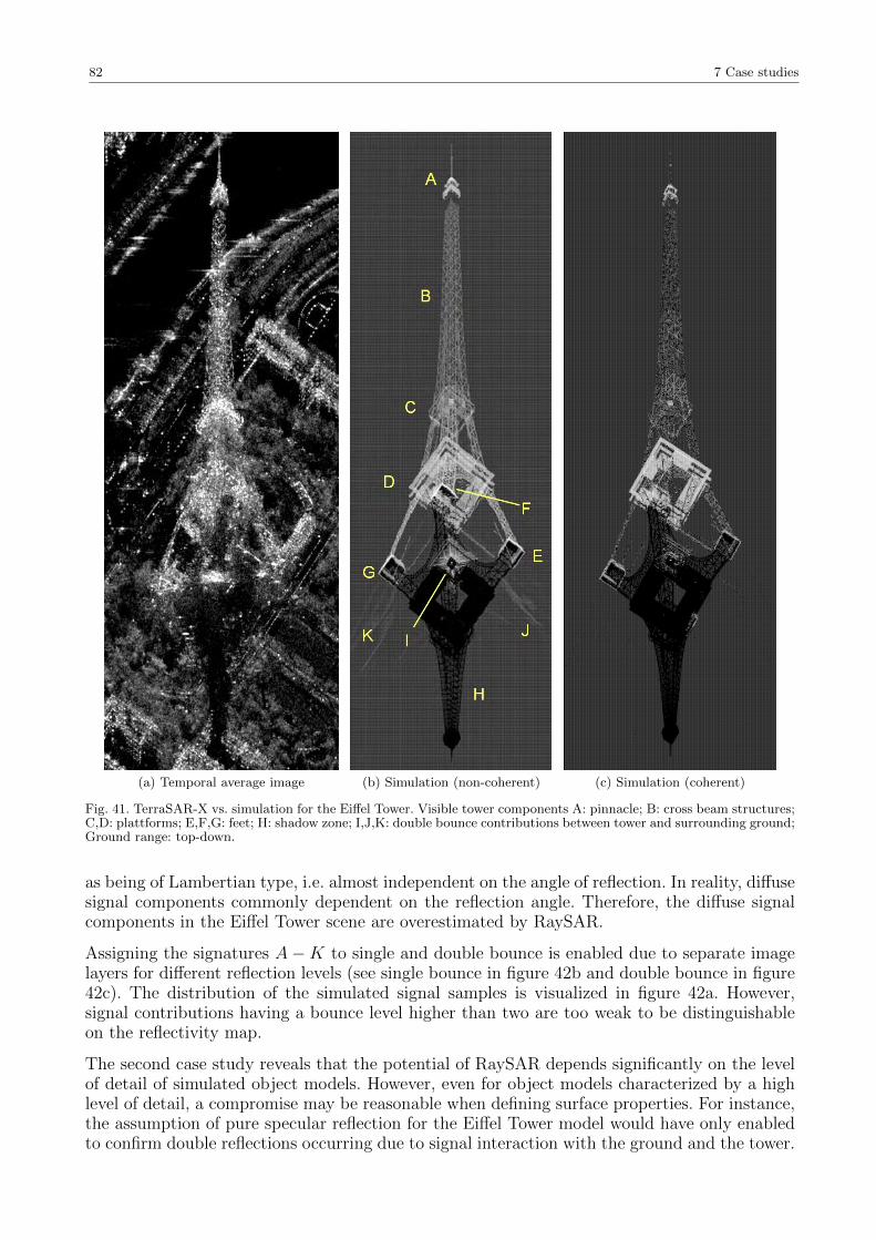
82 7 Case studies
(a) Temporal average image (b) Simulation (non-coherent) (c) Simulation (coherent)
Fig. 41. TerraSAR-X vs. simulation for the Eiffel Tower. Visible tower components A: pinnacle; B: cross beam structures;C,D: plattforms; E,F,G: feet; H: shadow zone; I,J,K: double bounce contributions between tower and surrounding ground;Ground range: top-down.
as being of Lambertian type, i.e. almost independent on the angle of reflection. In reality, diffusesignal components commonly dependent on the reflection angle. Therefore, the diffuse signalcomponents in the Eiffel Tower scene are overestimated by RaySAR.
Assigning the signatures A−K to single and double bounce is enabled due to separate imagelayers for different reflection levels (see single bounce in figure 42b and double bounce in figure42c). The distribution of the simulated signal samples is visualized in figure 42a. However,signal contributions having a bounce level higher than two are too weak to be distinguishableon the reflectivity map.
The second case study reveals that the potential of RaySAR depends significantly on the levelof detail of simulated object models. However, even for object models characterized by a highlevel of detail, a compromise may be reasonable when defining surface properties. For instance,the assumption of pure specular reflection for the Eiffel Tower model would have only enabledto confirm double reflections occurring due to signal interaction with the ground and the tower.
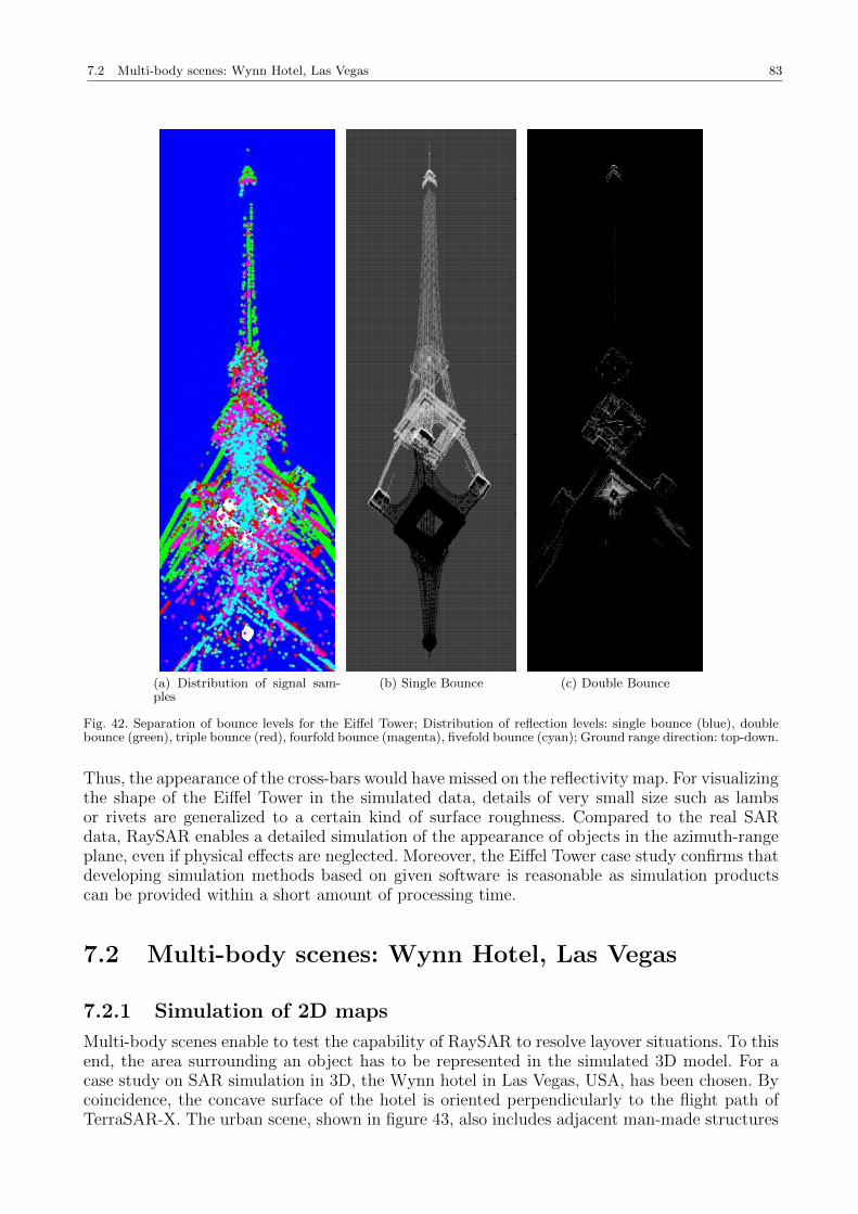
7.2 Multi-body scenes: Wynn Hotel, Las Vegas 83
(a) Distribution of signal sam-ples
(b) Single Bounce (c) Double Bounce
Fig. 42. Separation of bounce levels for the Eiffel Tower; Distribution of reflection levels: single bounce (blue), doublebounce (green), triple bounce (red), fourfold bounce (magenta), fivefold bounce (cyan); Ground range direction: top-down.
Thus, the appearance of the cross-bars would have missed on the reflectivity map. For visualizingthe shape of the Eiffel Tower in the simulated data, details of very small size such as lambsor rivets are generalized to a certain kind of surface roughness. Compared to the real SARdata, RaySAR enables a detailed simulation of the appearance of objects in the azimuth-rangeplane, even if physical effects are neglected. Moreover, the Eiffel Tower case study confirms thatdeveloping simulation methods based on given software is reasonable as simulation productscan be provided within a short amount of processing time.
7.2 Multi-body scenes: Wynn Hotel, Las Vegas
7.2.1 Simulation of 2D maps
Multi-body scenes enable to test the capability of RaySAR to resolve layover situations. To thisend, the area surrounding an object has to be represented in the simulated 3D model. For acase study on SAR simulation in 3D, the Wynn hotel in Las Vegas, USA, has been chosen. Bycoincidence, the concave surface of the hotel is oriented perpendicularly to the flight path ofTerraSAR-X. The urban scene, shown in figure 43, also includes adjacent man-made structures
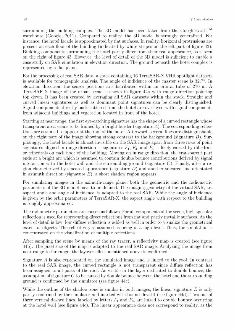
84 7 Case studies
surrounding the building complex. The 3D model has been taken from the Google EarthTM
warehouse (Google, 2011). Compared to reality, the 3D model is strongly generalized. Forinstance, the hotel facade is approximated by flat surfaces. In reality, horizontal protrusions arepresent on each floor of the building (indicated by white stripes on the left part of figure 43).Building components surrounding the hotel partly differ from their real appearance, as is seenon the right of figure 43. However, the level of detail of the 3D model is sufficient to enable acase study on SAR simulation in elevation direction. The ground beneath the hotel complex isrepresented by a flat plane.
For the processing of real SAR data, a stack containing 16 TerraSAR-X VHR spotlight datasetsis available for tomographic analysis. The angle of indidence of the master scene is 32.7. Inelevation direction, the sensor positions are distributed within an orbital tube of 270 m. ATerraSAR-X image of the urban scene is shown in figure 44a with range direction pointingtop down. It has been created by averaging all SAR datasets within the stack. Straight andcurved linear signatures as well as dominant point signatures can be clearly distinguished.Signal components directly backscattered from the hotel are overlayed with signal componentsfrom adjacent buildings and vegetation located in front of the hotel.
Starting at near range, the first eye-catching signature has the shape of a curved rectangle whosetransparent area seems to be framed by a bright border (signature A). The corresponding reflec-tions are assumed to appear at the roof of the hotel. Afterward, several lines are distinguishableon the right part of the image showing strong contrast to the background (signature B). Sur-prisingly, the hotel facade is almost invisible on the SAR image apart from three rows of pointsignatures aligned in range direction – signatures F1, F2, and F3 – likely caused by dihedralsor trihedrals on each floor of the building. Moving on in range direction, the transparent partends at a bright arc which is assumed to contain double bounce contributions derived by signalinteraction with the hotel wall and the surrounding ground (signature C). Finally, after a re-gion characterized by smeared appearance (signature D) and another smeared line orientatedin azimuth direction (signature E), a short shadow region appears.
For simulating images in the azimuth-range plane, both the geometric and the radiometricparameters of the 3D model have to be defined. The imaging geometry of the virtual SAR, i.e.aspect angle and angle of incidence, is adapted to the real SAR. While the angle of incidenceis given by the orbit parameters of TerraSAR-X, the aspect angle with respect to the buildingis roughly approximated.
The radiometric parameters are chosen as follows. For all components of the scene, high specularreflection is used for representing direct reflections from flat and partly metallic surfaces. As thelevel of detail is low, low diffuse reflection is added as well in order to visualize the geometricalextent of objects. The reflectivity is assumed as being of a high level. Thus, the simulation isconcentrated on the visualization of multiple reflections.
After sampling the scene by means of the ray tracer, a reflectivity map is created (see figure44b). The pixel size of the map is adapted to the real SAR image. Analyzing the image fromnear range to far range, the layover effect mentioned above is confirmed.
Signature A is also represented on the simulated image and is linked to the roof. In contrastto the real SAR image, the curved rectangle is not transparent since diffuse reflection hasbeen assigned to all parts of the roof. As visible in the layer dedicated to double bounce, theassumption of signature C to be caused by double bounce between the hotel and the surroundingground is confirmed by the simulator (see figure 44c).
While the outline of the shadow zone is similar in both images, the linear signature E is onlypartly confirmed by the simulator and marked with bounce level 4 (see figure 44d). Two out ofthree vertical dashed lines, labeled by letters F1 and F3, are linked to double bounce occurringat the hotel wall (see figure 44c). The linear appearance does not correspond to reality, as the
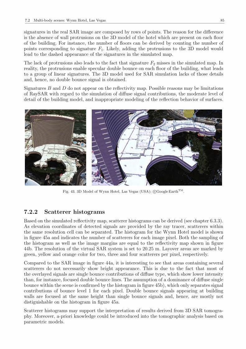
7.2 Multi-body scenes: Wynn Hotel, Las Vegas 85
signatures in the real SAR image are composed by rows of points. The reason for the differenceis the absence of wall protrusions on the 3D model of the hotel which are present on each floorof the building. For instance, the number of floors can be derived by counting the number ofpoints corresponding to signature F1. Likely, adding the protrusions to the 3D model wouldlead to the dashed appearance of the signatures in the simulated map.
The lack of protrusions also leads to the fact that signature F2 misses in the simulated map. Inreality, the protrusions enable specular double bounce on each floor of the building, what leadsto a group of linear signatures. The 3D model used for SAR simulation lacks of those detailsand, hence, no double bounce signal is obtained.
Signatures B and D do not appear on the reflectivity map. Possible reasons may be limitationsof RaySAR with regard to the simulation of diffuse signal contributions, the moderate level ofdetail of the building model, and inappropriate modeling of the reflection behavior of surfaces.
Fig. 43. 3D Model of Wynn Hotel, Las Vegas (USA); c©Google EarthTM.
7.2.2 Scatterer histograms
Based on the simulated reflectivity map, scatterer histograms can be derived (see chapter 6.3.3).As elevation coordinates of detected signals are provided by the ray tracer, scatterers withinthe same resolution cell can be separated. The histogram for the Wynn Hotel model is shownin figure 45a and indicates the number of scatterers for each image pixel. Both the sampling ofthe histogram as well as the image margins are equal to the reflectivity map shown in figure44b. The resolution of the virtual SAR system is set to 20.25 m. Layover areas are marked bygreen, yellow and orange color for two, three and four scatterers per pixel, respectively.
Compared to the SAR image in figure 44a, it is interesting to see that areas containing severalscatterers do not necessarily show bright appearance. This is due to the fact that most ofthe overlayed signals are single bounce contributions of diffuse type, which show lower intensitythan, for instance, focused double bounce lines. The assumption of a dominance of diffuse singlebounce within the scene is confirmed by the histogram in figure 45b), which only separates signalcontributions of bounce level 1 for each pixel. Double bounce signals appearing at buildingwalls are focused at the same height than single bounce signals and, hence, are mostly notdistiguishable on the histogram in figure 45a.
Scatterer histograms may support the interpretation of results derived from 3D SAR tomogra-phy. Moreover, a-priori knowledge could be introduced into the tomographic analysis based onparametric models.
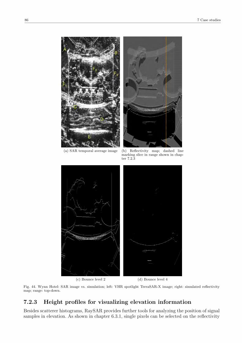
86 7 Case studies
(a) SAR temporal average image (b) Reflectivity map; dashed linemarking slice in range shown in chap-ter 7.2.3
(c) Bounce level 2 (d) Bounce level 4
Fig. 44. Wynn Hotel: SAR image vs. simulation; left: VHR spotlight TerraSAR-X image; right: simulated reflectivitymap; range: top-down.
7.2.3 Height profiles for visualizing elevation information
Besides scatterer histograms, RaySAR provides further tools for analyzing the position of signalsamples in elevation. As shown in chapter 6.3.1, single pixels can be selected on the reflectivity
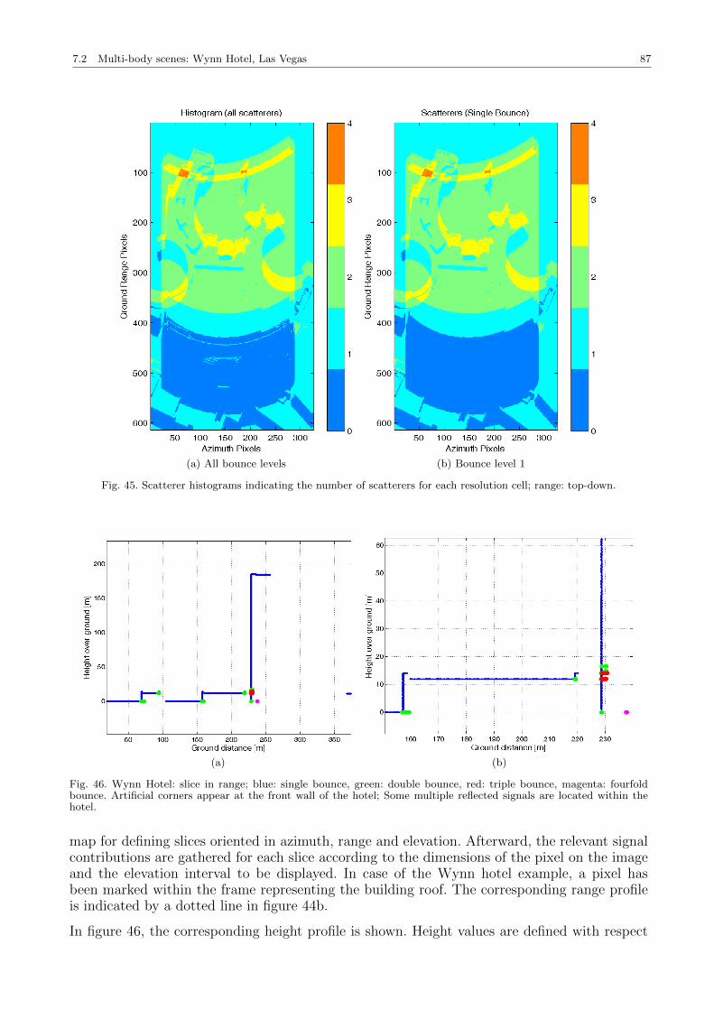
7.2 Multi-body scenes: Wynn Hotel, Las Vegas 87
(a) All bounce levels (b) Bounce level 1
Fig. 45. Scatterer histograms indicating the number of scatterers for each resolution cell; range: top-down.
(a) (b)
Fig. 46. Wynn Hotel: slice in range; blue: single bounce, green: double bounce, red: triple bounce, magenta: fourfoldbounce. Artificial corners appear at the front wall of the hotel; Some multiple reflected signals are located within thehotel.
map for defining slices oriented in azimuth, range and elevation. Afterward, the relevant signalcontributions are gathered for each slice according to the dimensions of the pixel on the imageand the elevation interval to be displayed. In case of the Wynn hotel example, a pixel hasbeen marked within the frame representing the building roof. The corresponding range profileis indicated by a dotted line in figure 44b.
In figure 46, the corresponding height profile is shown. Height values are defined with respect
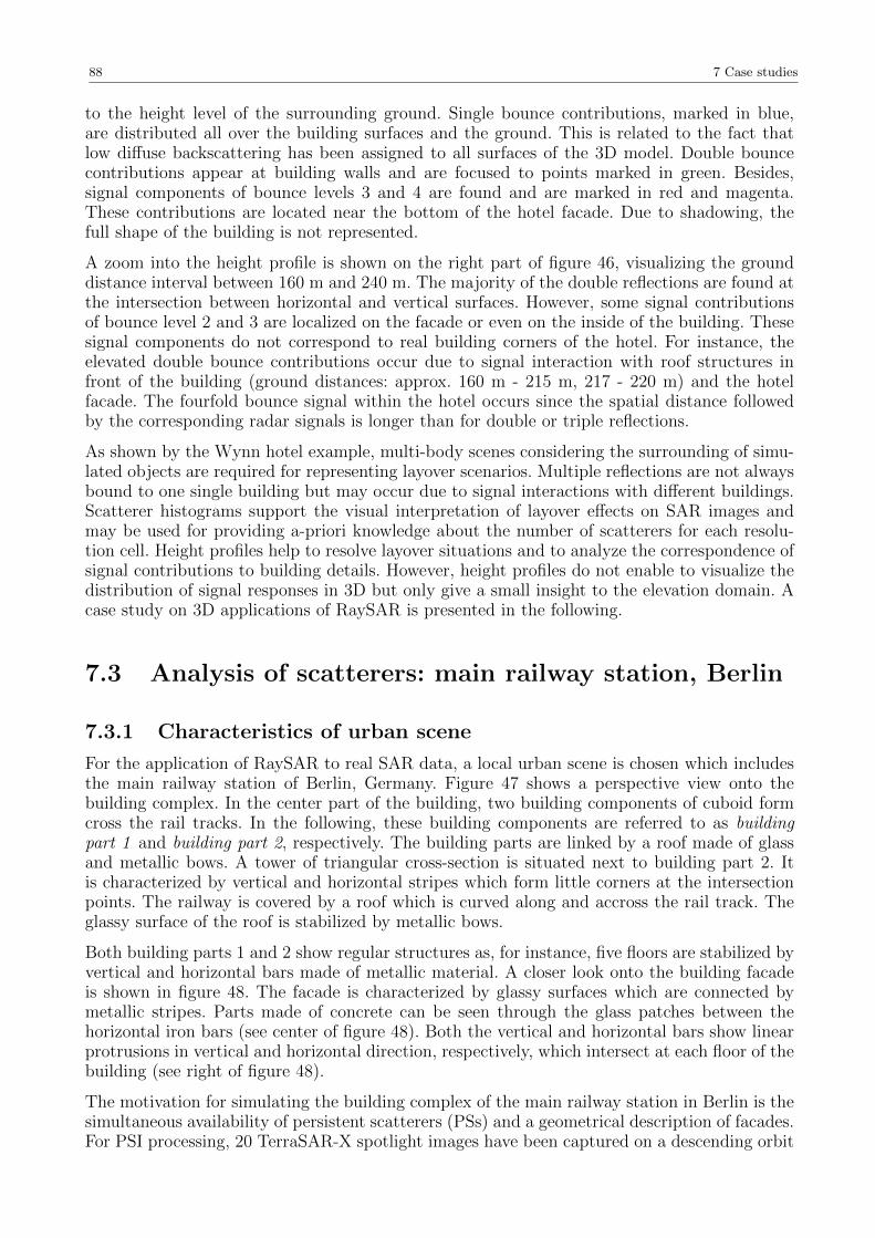
88 7 Case studies
to the height level of the surrounding ground. Single bounce contributions, marked in blue,are distributed all over the building surfaces and the ground. This is related to the fact thatlow diffuse backscattering has been assigned to all surfaces of the 3D model. Double bouncecontributions appear at building walls and are focused to points marked in green. Besides,signal components of bounce levels 3 and 4 are found and are marked in red and magenta.These contributions are located near the bottom of the hotel facade. Due to shadowing, thefull shape of the building is not represented.
A zoom into the height profile is shown on the right part of figure 46, visualizing the grounddistance interval between 160 m and 240 m. The majority of the double reflections are found atthe intersection between horizontal and vertical surfaces. However, some signal contributionsof bounce level 2 and 3 are localized on the facade or even on the inside of the building. Thesesignal components do not correspond to real building corners of the hotel. For instance, theelevated double bounce contributions occur due to signal interaction with roof structures infront of the building (ground distances: approx. 160 m - 215 m, 217 - 220 m) and the hotelfacade. The fourfold bounce signal within the hotel occurs since the spatial distance followedby the corresponding radar signals is longer than for double or triple reflections.
As shown by the Wynn hotel example, multi-body scenes considering the surrounding of simu-lated objects are required for representing layover scenarios. Multiple reflections are not alwaysbound to one single building but may occur due to signal interactions with different buildings.Scatterer histograms support the visual interpretation of layover effects on SAR images andmay be used for providing a-priori knowledge about the number of scatterers for each resolu-tion cell. Height profiles help to resolve layover situations and to analyze the correspondence ofsignal contributions to building details. However, height profiles do not enable to visualize thedistribution of signal responses in 3D but only give a small insight to the elevation domain. Acase study on 3D applications of RaySAR is presented in the following.
7.3 Analysis of scatterers: main railway station, Berlin
7.3.1 Characteristics of urban scene
For the application of RaySAR to real SAR data, a local urban scene is chosen which includesthe main railway station of Berlin, Germany. Figure 47 shows a perspective view onto thebuilding complex. In the center part of the building, two building components of cuboid formcross the rail tracks. In the following, these building components are referred to as buildingpart 1 and building part 2, respectively. The building parts are linked by a roof made of glassand metallic bows. A tower of triangular cross-section is situated next to building part 2. Itis characterized by vertical and horizontal stripes which form little corners at the intersectionpoints. The railway is covered by a roof which is curved along and accross the rail track. Theglassy surface of the roof is stabilized by metallic bows.
Both building parts 1 and 2 show regular structures as, for instance, five floors are stabilized byvertical and horizontal bars made of metallic material. A closer look onto the building facadeis shown in figure 48. The facade is characterized by glassy surfaces which are connected bymetallic stripes. Parts made of concrete can be seen through the glass patches between thehorizontal iron bars (see center of figure 48). Both the vertical and horizontal bars show linearprotrusions in vertical and horizontal direction, respectively, which intersect at each floor of thebuilding (see right of figure 48).
The motivation for simulating the building complex of the main railway station in Berlin is thesimultaneous availability of persistent scatterers (PSs) and a geometrical description of facades.For PSI processing, 20 TerraSAR-X spotlight images have been captured on a descending orbit
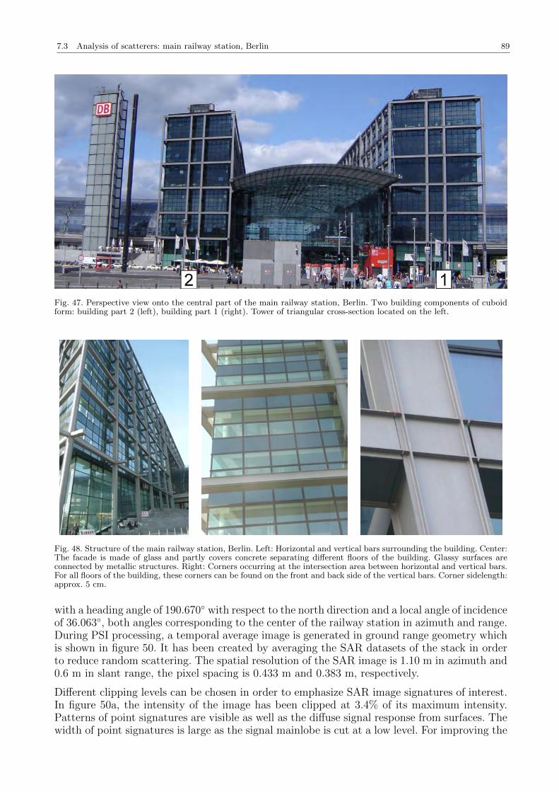
7.3 Analysis of scatterers: main railway station, Berlin 89
Fig. 47. Perspective view onto the central part of the main railway station, Berlin. Two building components of cuboidform: building part 2 (left), building part 1 (right). Tower of triangular cross-section located on the left.
Fig. 48. Structure of the main railway station, Berlin. Left: Horizontal and vertical bars surrounding the building. Center:The facade is made of glass and partly covers concrete separating different floors of the building. Glassy surfaces areconnected by metallic structures. Right: Corners occurring at the intersection area between horizontal and vertical bars.For all floors of the building, these corners can be found on the front and back side of the vertical bars. Corner sidelength:approx. 5 cm.
with a heading angle of 190.670 with respect to the north direction and a local angle of incidenceof 36.063, both angles corresponding to the center of the railway station in azimuth and range.During PSI processing, a temporal average image is generated in ground range geometry whichis shown in figure 50. It has been created by averaging the SAR datasets of the stack in orderto reduce random scattering. The spatial resolution of the SAR image is 1.10 m in azimuth and0.6 m in slant range, the pixel spacing is 0.433 m and 0.383 m, respectively.
Different clipping levels can be chosen in order to emphasize SAR image signatures of interest.In figure 50a, the intensity of the image has been clipped at 3.4% of its maximum intensity.Patterns of point signatures are visible as well as the diffuse signal response from surfaces. Thewidth of point signatures is large as the signal mainlobe is cut at a low level. For improving the
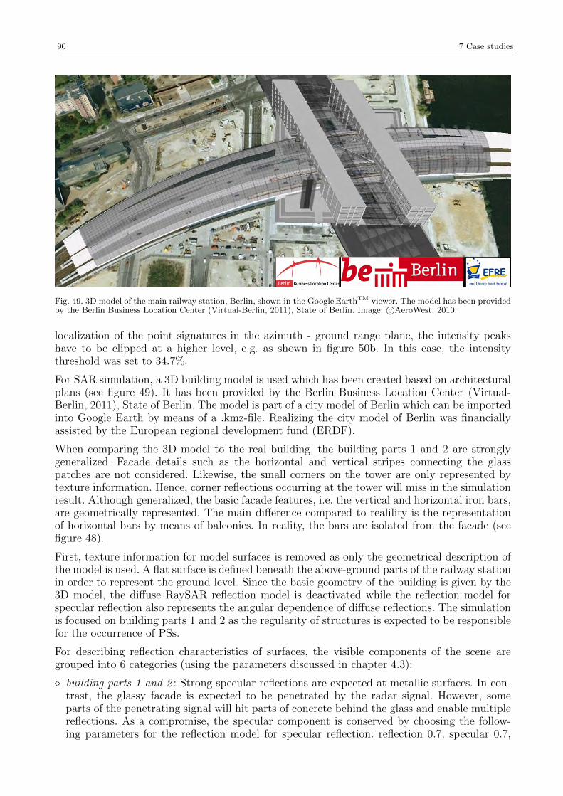
90 7 Case studies
Fig. 49. 3D model of the main railway station, Berlin, shown in the Google EarthTM viewer. The model has been providedby the Berlin Business Location Center (Virtual-Berlin, 2011), State of Berlin. Image: c©AeroWest, 2010.
localization of the point signatures in the azimuth - ground range plane, the intensity peakshave to be clipped at a higher level, e.g. as shown in figure 50b. In this case, the intensitythreshold was set to 34.7%.
For SAR simulation, a 3D building model is used which has been created based on architecturalplans (see figure 49). It has been provided by the Berlin Business Location Center (Virtual-Berlin, 2011), State of Berlin. The model is part of a city model of Berlin which can be importedinto Google Earth by means of a .kmz-file. Realizing the city model of Berlin was financiallyassisted by the European regional development fund (ERDF).
When comparing the 3D model to the real building, the building parts 1 and 2 are stronglygeneralized. Facade details such as the horizontal and vertical stripes connecting the glasspatches are not considered. Likewise, the small corners on the tower are only represented bytexture information. Hence, corner reflections occurring at the tower will miss in the simulationresult. Although generalized, the basic facade features, i.e. the vertical and horizontal iron bars,are geometrically represented. The main difference compared to realility is the representationof horizontal bars by means of balconies. In reality, the bars are isolated from the facade (seefigure 48).
First, texture information for model surfaces is removed as only the geometrical description ofthe model is used. A flat surface is defined beneath the above-ground parts of the railway stationin order to represent the ground level. Since the basic geometry of the building is given by the3D model, the diffuse RaySAR reflection model is deactivated while the reflection model forspecular reflection also represents the angular dependence of diffuse reflections. The simulationis focused on building parts 1 and 2 as the regularity of structures is expected to be responsiblefor the occurrence of PSs.
For describing reflection characteristics of surfaces, the visible components of the scene aregrouped into 6 categories (using the parameters discussed in chapter 4.3):
building parts 1 and 2 : Strong specular reflections are expected at metallic surfaces. In con-trast, the glassy facade is expected to be penetrated by the radar signal. However, someparts of the penetrating signal will hit parts of concrete behind the glass and enable multiplereflections. As a compromise, the specular component is conserved by choosing the follow-ing parameters for the reflection model for specular reflection: reflection 0.7, specular 0.7,
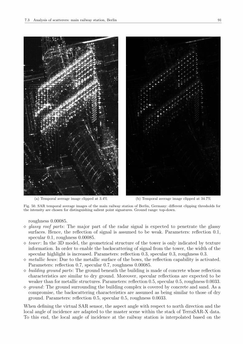
7.3 Analysis of scatterers: main railway station, Berlin 91
(a) Temporal average image clipped at 3.4% (b) Temporal average image clipped at 34.7%
Fig. 50. SAR temporal average images of the main railway station of Berlin, Germany: different clipping thresholds forthe intensity are chosen for distinguishing salient point signatures. Ground range: top-down.
roughness 0.00085. glassy roof parts : The major part of the radar signal is expected to penetrate the glassy
surfaces. Hence, the reflection of signal is assumed to be weak. Parameters: reflection 0.1,specular 0.1, roughness 0.00085. tower : In the 3D model, the geometrical structure of the tower is only indicated by texture
information. In order to enable the backscattering of signal from the tower, the width of thespecular highlight is increased. Parameters: reflection 0.3, specular 0.3, roughness 0.3. metallic bows : Due to the metallic surface of the bows, the reflection capability is activated.
Parameters: reflection 0.7, specular 0.7, roughness 0.00085. building ground parts : The ground beneath the building is made of concrete whose reflection
characteristics are similar to dry ground. Moreover, specular reflections are expected to beweaker than for metallic structures. Parameters: reflection 0.5, specular 0.5, roughness 0.0033. ground : The ground surrounding the building complex is covered by concrete and sand. As a
compromise, the backscattering characteristics are assumed as being similar to those of dryground. Parameters: reflection 0.5, specular 0.5, roughness 0.0033.
When defining the virtual SAR sensor, the aspect angle with respect to north direction and thelocal angle of incidence are adapted to the master scene within the stack of TerraSAR-X data.To this end, the local angle of incidence at the railway station is interpolated based on the
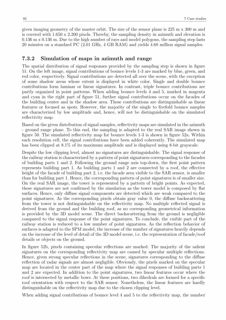
92 7 Case studies
given imaging geometry of the master orbit. The size of the sensor plane is 225 m x 300 m andis covered with 1.650 x 2.200 pixels. Thereby, the sampling density in azimuth and elevation is0.136 m x 0.136 m. Due to the high number of rays and model polygons, the sampling step lasts20 minutes on a standard PC (2.01 GHz, 4 GB RAM) and yields 4.68 million signal samples.
7.3.2 Simulation of maps in azimuth and range
The spatial distribution of signal responses provided by the sampling step is shown in figure51. On the left image, signal contributions of bounce levels 1-3 are marked by blue, green, andred color, respectively. Signal contributions are detected all over the scene, with the exceptionof some shadow areas whose extent is displayed in white color. Single and double bouncecontributions form laminar or linear signatures. In contrast, triple bounce contributions arepartly organized in point patterns. When adding bounce levels 4 and 5, marked in magentaand cyan in the right part of figure 51, further signal contributions occur on the facades ofthe building center and in the shadow area. These contributions are distinguishable as linearfeatures or focused as spots. However, the majority of the single to fivefold bounce samplesare characterized by low amplitude and, hence, will not be distinguishable on the simulatedreflectivity map.
Based on the given distribution of signal samples, reflectivity maps are simulated in the azimuth- ground range plane. To this end, the sampling is adapted to the real SAR image shown infigure 50. The simulated reflectivity map for bounce levels 1-3 is shown in figure 52a. Withineach resolution cell, the signal contributions have been added coherently. The simulated maphas been clipped at 8.1% of its maximum amplitude and is displayed using 8-bit grayscale.
Despite the low clipping level, almost no signatures are distinguishable. The signal response ofthe railway station is characterized by a pattern of point signatures corresponding to the facadesof building parts 1 and 2. Following the ground range axis top-down, the first point patternrepresents building part 1. As building parts 1 and 2 are connected by a roof, the effectiveheight of the facade of building part 2, i.e. the facade area visible to the SAR sensor, is smallerthan for building part 1. Hence, the corresponding pattern of point signatures is of smaller size.On the real SAR image, the tower is represented by a pattern of bright points. As expected,these signatures are not confirmed by the simulation as the tower model is composed by flatsurfaces. Hence, only diffuse signal components are detected which are weak compared to thepoint signatures. As the corresponding pixels obtain gray value 0, the diffuse backscatteringfrom the tower is not distinguishable on the reflectivity map. No multiple reflected signal isderived from the ground and the building roof, as no corresponding geometrical informationis provided by the 3D model scene. The direct backscattering from the ground is negligiblecompared to the signal response of the point signatures. To conclude, the visible part of therailway station is reduced to a low number of point signatures. As the reflection behavior ofsurfaces is adapted to the SPM model, the increase of the number of signatures heavily dependson the increase of the level of detail of the 3D model scene, i.e. the representation of facade/roofdetails or objects on the ground.
In figure 52b, pixels containing specular reflections are marked. The majority of the salientsignatures on the corresponding reflectivity map are caused by specular multiple reflections.Hence, given strong specular reflections in the scene, signatures corresponding to the diffusereflection of radar signals are almost negligible. Obviously, the pixels marked on the specularmap are located in the center part of the map where the signal responses of building parts 1and 2 are expected. In addition to the point signatures, two linear features occur where theroof is intersected by metallic bows. At these positions, two dihedrals are formed for a specificroof orientation with respect to the SAR sensor. Nonetheless, the linear features are hardlydistinguishable on the reflectivity map due to the chosen clipping level.
When adding signal contributions of bounce level 4 and 5 to the reflectivity map, the number
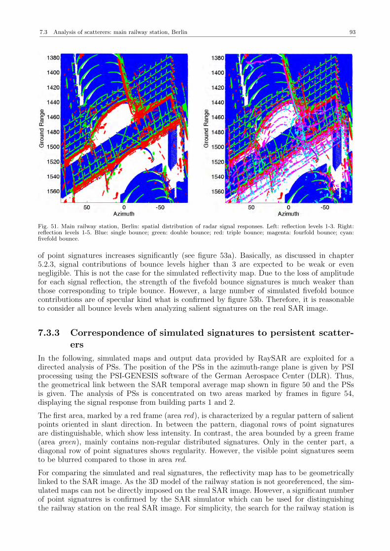
7.3 Analysis of scatterers: main railway station, Berlin 93
Fig. 51. Main railway station, Berlin: spatial distribution of radar signal responses. Left: reflection levels 1-3. Right:reflection levels 1-5. Blue: single bounce; green: double bounce; red: triple bounce; magenta: fourfold bounce; cyan:fivefold bounce.
of point signatures increases significantly (see figure 53a). Basically, as discussed in chapter5.2.3, signal contributions of bounce levels higher than 3 are expected to be weak or evennegligible. This is not the case for the simulated reflectivity map. Due to the loss of amplitudefor each signal reflection, the strength of the fivefold bounce signatures is much weaker thanthose corresponding to triple bounce. However, a large number of simulated fivefold bouncecontributions are of specular kind what is confirmed by figure 53b. Therefore, it is reasonableto consider all bounce levels when analyzing salient signatures on the real SAR image.
7.3.3 Correspondence of simulated signatures to persistent scatter-ers
In the following, simulated maps and output data provided by RaySAR are exploited for adirected analysis of PSs. The position of the PSs in the azimuth-range plane is given by PSIprocessing using the PSI-GENESIS software of the German Aerospace Center (DLR). Thus,the geometrical link between the SAR temporal average map shown in figure 50 and the PSsis given. The analysis of PSs is concentrated on two areas marked by frames in figure 54,displaying the signal response from building parts 1 and 2.
The first area, marked by a red frame (area red), is characterized by a regular pattern of salientpoints oriented in slant direction. In between the pattern, diagonal rows of point signaturesare distinguishable, which show less intensity. In contrast, the area bounded by a green frame(area green), mainly contains non-regular distributed signatures. Only in the center part, adiagonal row of point signatures shows regularity. However, the visible point signatures seemto be blurred compared to those in area red.
For comparing the simulated and real signatures, the reflectivity map has to be geometricallylinked to the SAR image. As the 3D model of the railway station is not georeferenced, the sim-ulated maps can not be directly imposed on the real SAR image. However, a significant numberof point signatures is confirmed by the SAR simulator which can be used for distinguishingthe railway station on the real SAR image. For simplicity, the search for the railway station is
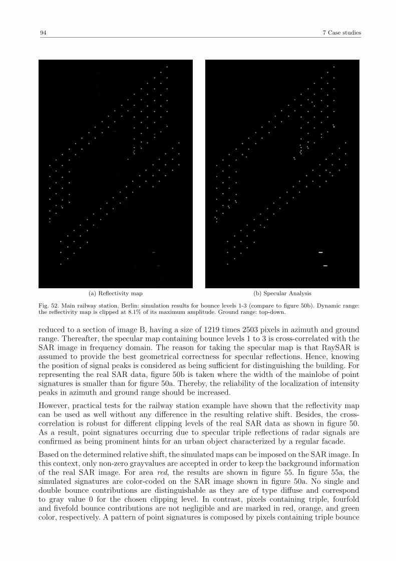
94 7 Case studies
(a) Reflectivity map (b) Specular Analysis
Fig. 52. Main railway station, Berlin: simulation results for bounce levels 1-3 (compare to figure 50b). Dynamic range:the reflectivity map is clipped at 8.1% of its maximum amplitude. Ground range: top-down.
reduced to a section of image B, having a size of 1219 times 2503 pixels in azimuth and groundrange. Thereafter, the specular map containing bounce levels 1 to 3 is cross-correlated with theSAR image in frequency domain. The reason for taking the specular map is that RaySAR isassumed to provide the best geometrical correctness for specular reflections. Hence, knowingthe position of signal peaks is considered as being sufficient for distinguishing the building. Forrepresenting the real SAR data, figure 50b is taken where the width of the mainlobe of pointsignatures is smaller than for figure 50a. Thereby, the reliability of the localization of intensitypeaks in azimuth and ground range should be increased.
However, practical tests for the railway station example have shown that the reflectivity mapcan be used as well without any difference in the resulting relative shift. Besides, the cross-correlation is robust for different clipping levels of the real SAR data as shown in figure 50.As a result, point signatures occurring due to specular triple reflections of radar signals areconfirmed as being prominent hints for an urban object characterized by a regular facade.
Based on the determined relative shift, the simulated maps can be imposed on the SAR image. Inthis context, only non-zero grayvalues are accepted in order to keep the background informationof the real SAR image. For area red, the results are shown in figure 55. In figure 55a, thesimulated signatures are color-coded on the SAR image shown in figure 50a. No single anddouble bounce contributions are distinguishable as they are of type diffuse and correspondto gray value 0 for the chosen clipping level. In contrast, pixels containing triple, fourfoldand fivefold bounce contributions are not negligible and are marked in red, orange, and greencolor, respectively. A pattern of point signatures is composed by pixels containing triple bounce
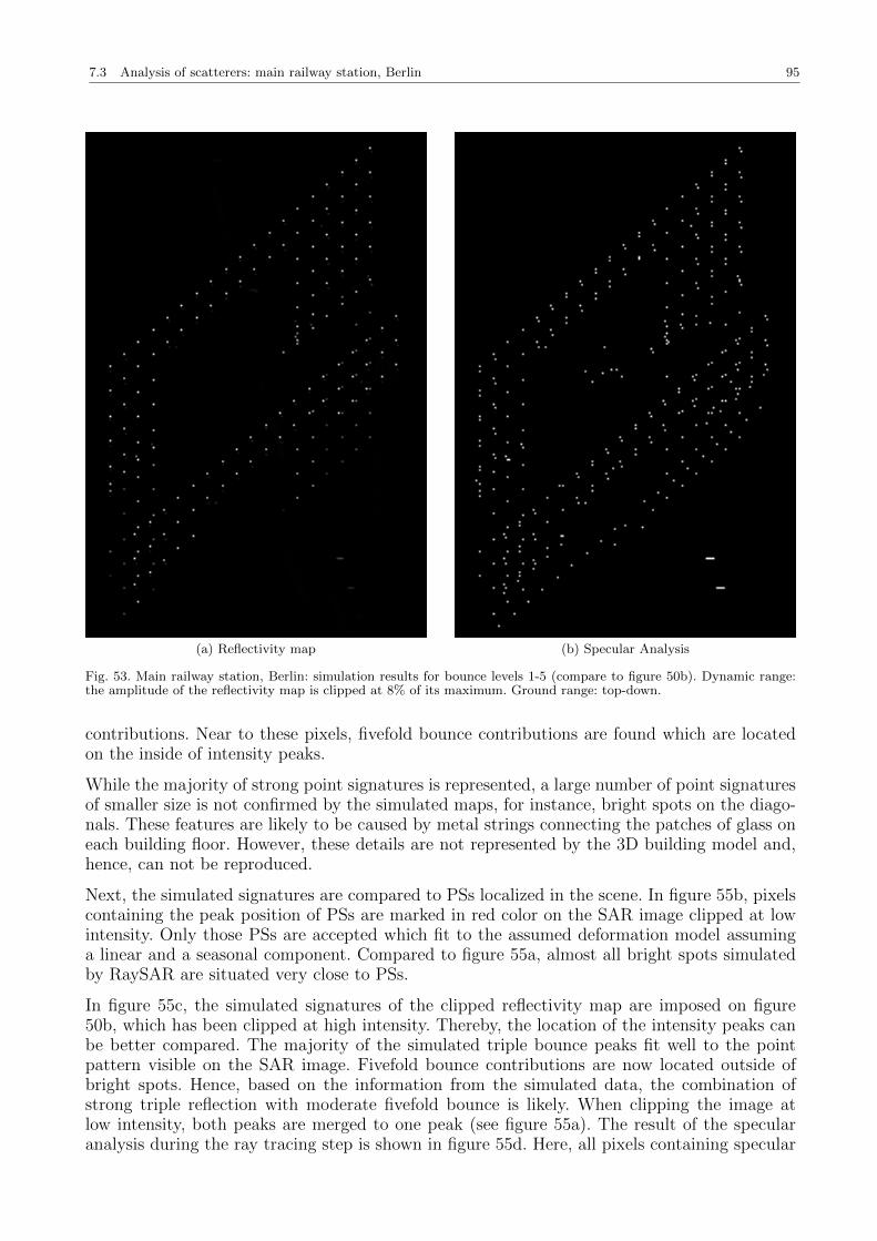
7.3 Analysis of scatterers: main railway station, Berlin 95
(a) Reflectivity map (b) Specular Analysis
Fig. 53. Main railway station, Berlin: simulation results for bounce levels 1-5 (compare to figure 50b). Dynamic range:the amplitude of the reflectivity map is clipped at 8% of its maximum. Ground range: top-down.
contributions. Near to these pixels, fivefold bounce contributions are found which are locatedon the inside of intensity peaks.
While the majority of strong point signatures is represented, a large number of point signaturesof smaller size is not confirmed by the simulated maps, for instance, bright spots on the diago-nals. These features are likely to be caused by metal strings connecting the patches of glass oneach building floor. However, these details are not represented by the 3D building model and,hence, can not be reproduced.
Next, the simulated signatures are compared to PSs localized in the scene. In figure 55b, pixelscontaining the peak position of PSs are marked in red color on the SAR image clipped at lowintensity. Only those PSs are accepted which fit to the assumed deformation model assuminga linear and a seasonal component. Compared to figure 55a, almost all bright spots simulatedby RaySAR are situated very close to PSs.
In figure 55c, the simulated signatures of the clipped reflectivity map are imposed on figure50b, which has been clipped at high intensity. Thereby, the location of the intensity peaks canbe better compared. The majority of the simulated triple bounce peaks fit well to the pointpattern visible on the SAR image. Fivefold bounce contributions are now located outside ofbright spots. Hence, based on the information from the simulated data, the combination ofstrong triple reflection with moderate fivefold bounce is likely. When clipping the image atlow intensity, both peaks are merged to one peak (see figure 55a). The result of the specularanalysis during the ray tracing step is shown in figure 55d. Here, all pixels containing specular
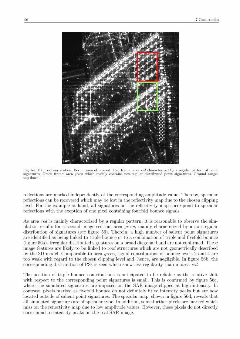
96 7 Case studies
Fig. 54. Main railway station, Berlin: area of interest. Red frame: area red characterized by a regular pattern of pointsignatures. Green frame: area green which mainly contains non-regular distributed point signatures. Ground range:top-down.
reflections are marked independently of the corresponding amplitude value. Thereby, specularreflections can be recovered which may be lost in the reflectivity map due to the chosen clippinglevel. For the example at hand, all signatures on the reflectivity map correspond to specularreflections with the exeption of one pixel containing fourfold bounce signals.
As area red is mainly characterized by a regular pattern, it is reasonable to observe the sim-ulation results for a second image section, area green, mainly characterized by a non-regulardistribution of signatures (see figure 56). Therein, a high number of salient point signaturesare identified as being linked to triple bounce or to a combination of triple and fivefold bounce(figure 56a). Irregular distributed signatures on a broad diagonal band are not confirmed. Theseimage features are likely to be linked to roof structures which are not geometrically describedby the 3D model. Comparable to area green, signal contributions of bounce levels 2 and 4 aretoo weak with regard to the chosen clipping level and, hence, are negligible. In figure 56b, thecorresponding distribution of PSs is seen which show less regularity than in area red.
The position of triple bounce contributions is anticipated to be reliable as the relative shiftwith respect to the corresponding point signatures is small. This is confirmed by figure 56c,where the simulated signatures are imposed on the SAR image clipped at high intensity. Incontrast, pixels marked as fivefold bounce do not definitely fit to intensity peaks but are nowlocated outside of salient point signatures. The specular map, shown in figure 56d, reveals thatall simulated signatures are of specular type. In addition, some further pixels are marked whichmiss on the reflectivity map due to low amplitude values. However, these pixels do not directlycorrespond to intensity peaks on the real SAR image.
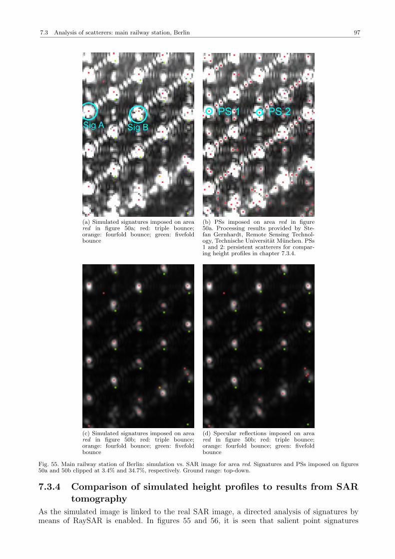
7.3 Analysis of scatterers: main railway station, Berlin 97
(a) Simulated signatures imposed on areared in figure 50a; red: triple bounce;orange: fourfold bounce; green: fivefoldbounce
(b) PSs imposed on area red in figure50a. Processing results provided by Ste-fan Gernhardt, Remote Sensing Technol-ogy, Technische Universitat Munchen. PSs1 and 2: persistent scatterers for compar-ing height profiles in chapter 7.3.4.
(c) Simulated signatures imposed on areared in figure 50b; red: triple bounce;orange: fourfold bounce; green: fivefoldbounce
(d) Specular reflections imposed on areared in figure 50b; red: triple bounce;orange: fourfold bounce; green: fivefoldbounce
Fig. 55. Main railway station of Berlin: simulation vs. SAR image for area red. Signatures and PSs imposed on figures50a and 50b clipped at 3.4% and 34.7%, respectively. Ground range: top-down.
7.3.4 Comparison of simulated height profiles to results from SARtomography
As the simulated image is linked to the real SAR image, a directed analysis of signatures bymeans of RaySAR is enabled. In figures 55 and 56, it is seen that salient point signatures
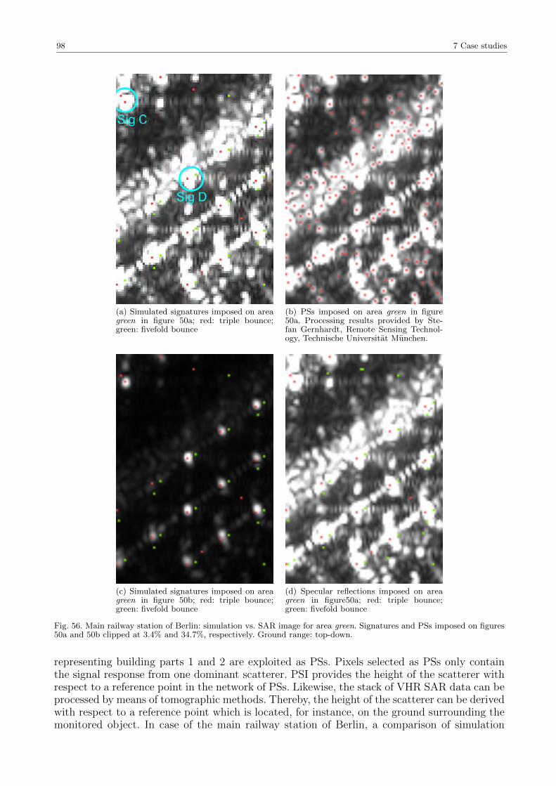
98 7 Case studies
(a) Simulated signatures imposed on areagreen in figure 50a; red: triple bounce;green: fivefold bounce
(b) PSs imposed on area green in figure50a. Processing results provided by Ste-fan Gernhardt, Remote Sensing Technol-ogy, Technische Universitat Munchen.
(c) Simulated signatures imposed on areagreen in figure 50b; red: triple bounce;green: fivefold bounce
(d) Specular reflections imposed on areagreen in figure50a; red: triple bounce;green: fivefold bounce
Fig. 56. Main railway station of Berlin: simulation vs. SAR image for area green. Signatures and PSs imposed on figures50a and 50b clipped at 3.4% and 34.7%, respectively. Ground range: top-down.
representing building parts 1 and 2 are exploited as PSs. Pixels selected as PSs only containthe signal response from one dominant scatterer. PSI provides the height of the scatterer withrespect to a reference point in the network of PSs. Likewise, the stack of VHR SAR data can beprocessed by means of tomographic methods. Thereby, the height of the scatterer can be derivedwith respect to a reference point which is located, for instance, on the ground surrounding themonitored object. In case of the main railway station of Berlin, a comparison of simulation
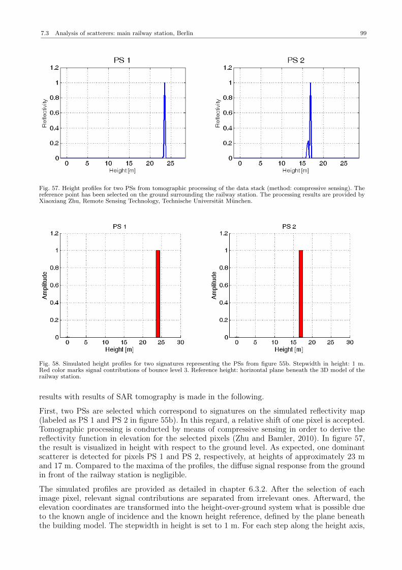
7.3 Analysis of scatterers: main railway station, Berlin 99
Fig. 57. Height profiles for two PSs from tomographic processing of the data stack (method: compressive sensing). Thereference point has been selected on the ground surrounding the railway station. The processing results are provided byXiaoxiang Zhu, Remote Sensing Technology, Technische Universitat Munchen.
Fig. 58. Simulated height profiles for two signatures representing the PSs from figure 55b. Stepwidth in height: 1 m.Red color marks signal contributions of bounce level 3. Reference height: horizontal plane beneath the 3D model of therailway station.
results with results of SAR tomography is made in the following.
First, two PSs are selected which correspond to signatures on the simulated reflectivity map(labeled as PS 1 and PS 2 in figure 55b). In this regard, a relative shift of one pixel is accepted.Tomographic processing is conducted by means of compressive sensing in order to derive thereflectivity function in elevation for the selected pixels (Zhu and Bamler, 2010). In figure 57,the result is visualized in height with respect to the ground level. As expected, one dominantscatterer is detected for pixels PS 1 and PS 2, respectively, at heights of approximately 23 mand 17 m. Compared to the maxima of the profiles, the diffuse signal response from the groundin front of the railway station is negligible.
The simulated profiles are provided as detailed in chapter 6.3.2. After the selection of eachimage pixel, relevant signal contributions are separated from irrelevant ones. Afterward, theelevation coordinates are transformed into the height-over-ground system what is possible dueto the known angle of incidence and the known height reference, defined by the plane beneaththe building model. The stepwidth in height is set to 1 m. For each step along the height axis,
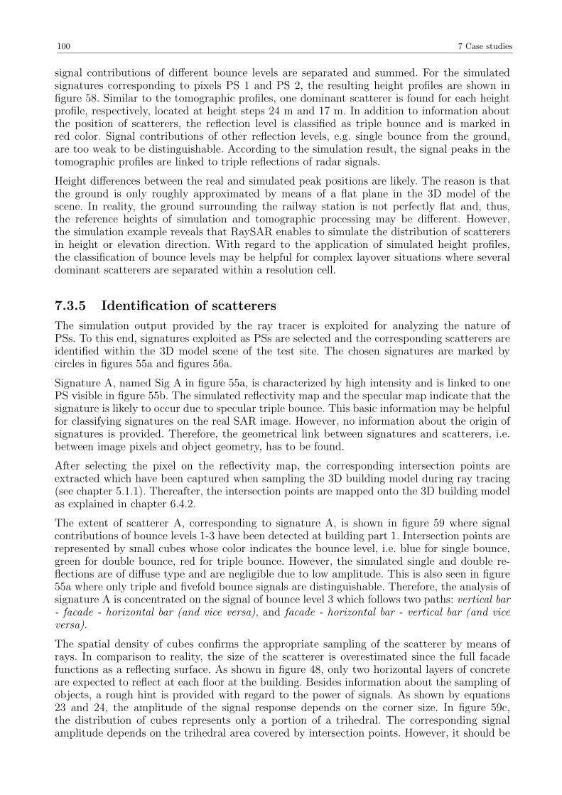
100 7 Case studies
signal contributions of different bounce levels are separated and summed. For the simulatedsignatures corresponding to pixels PS 1 and PS 2, the resulting height profiles are shown infigure 58. Similar to the tomographic profiles, one dominant scatterer is found for each heightprofile, respectively, located at height steps 24 m and 17 m. In addition to information aboutthe position of scatterers, the reflection level is classified as triple bounce and is marked inred color. Signal contributions of other reflection levels, e.g. single bounce from the ground,are too weak to be distinguishable. According to the simulation result, the signal peaks in thetomographic profiles are linked to triple reflections of radar signals.
Height differences between the real and simulated peak positions are likely. The reason is thatthe ground is only roughly approximated by means of a flat plane in the 3D model of thescene. In reality, the ground surrounding the railway station is not perfectly flat and, thus,the reference heights of simulation and tomographic processing may be different. However,the simulation example reveals that RaySAR enables to simulate the distribution of scatterersin height or elevation direction. With regard to the application of simulated height profiles,the classification of bounce levels may be helpful for complex layover situations where severaldominant scatterers are separated within a resolution cell.
7.3.5 Identification of scatterers
The simulation output provided by the ray tracer is exploited for analyzing the nature ofPSs. To this end, signatures exploited as PSs are selected and the corresponding scatterers areidentified within the 3D model scene of the test site. The chosen signatures are marked bycircles in figures 55a and figures 56a.
Signature A, named Sig A in figure 55a, is characterized by high intensity and is linked to onePS visible in figure 55b. The simulated reflectivity map and the specular map indicate that thesignature is likely to occur due to specular triple bounce. This basic information may be helpfulfor classifying signatures on the real SAR image. However, no information about the origin ofsignatures is provided. Therefore, the geometrical link between signatures and scatterers, i.e.between image pixels and object geometry, has to be found.
After selecting the pixel on the reflectivity map, the corresponding intersection points areextracted which have been captured when sampling the 3D building model during ray tracing(see chapter 5.1.1). Thereafter, the intersection points are mapped onto the 3D building modelas explained in chapter 6.4.2.
The extent of scatterer A, corresponding to signature A, is shown in figure 59 where signalcontributions of bounce levels 1-3 have been detected at building part 1. Intersection points arerepresented by small cubes whose color indicates the bounce level, i.e. blue for single bounce,green for double bounce, red for triple bounce. However, the simulated single and double re-flections are of diffuse type and are negligible due to low amplitude. This is also seen in figure55a where only triple and fivefold bounce signals are distinguishable. Therefore, the analysis ofsignature A is concentrated on the signal of bounce level 3 which follows two paths: vertical bar- facade - horizontal bar (and vice versa), and facade - horizontal bar - vertical bar (and viceversa).
The spatial density of cubes confirms the appropriate sampling of the scatterer by means ofrays. In comparison to reality, the size of the scatterer is overestimated since the full facadefunctions as a reflecting surface. As shown in figure 48, only two horizontal layers of concreteare expected to reflect at each floor at the building. Besides information about the sampling ofobjects, a rough hint is provided with regard to the power of signals. As shown by equations23 and 24, the amplitude of the signal response depends on the corner size. In figure 59c,the distribution of cubes represents only a portion of a trihedral. The corresponding signalamplitude depends on the trihedral area covered by intersection points. However, it should be
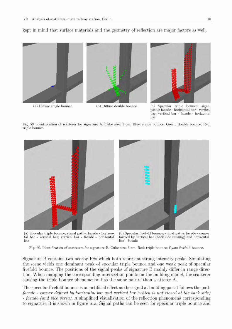
7.3 Analysis of scatterers: main railway station, Berlin 101
kept in mind that surface materials and the geometry of reflection are major factors as well.
(a) Diffuse single bounce (b) Diffuse double bounce (c) Specular triple bounce; signalpaths: facade - horizontal bar - verticalbar; vertical bar - facade - horizontalbar
Fig. 59. Identification of scatterer for signature A. Cube size: 5 cm. Blue: single bounce; Green: double bounce; Red:triple bounce.
(a) Specular triple bounce; signal paths: facade - horizon-tal bar - vertical bar; vertical bar - facade - horizontalbar
(b) Specular fivefold bounce; signal paths: facade - cornerformed by vertical bar (back side missing) and horizontalbar - facade
Fig. 60. Identification of scatterers for signature B. Cube size: 5 cm. Red: triple bounce; Cyan: fivefold bounce.
Signature B contains two nearby PSs which both represent strong intensity peaks. Simulatingthe scene yields one dominant peak of specular triple bounce and one weak peak of specularfivefold bounce. The positions of the signal peaks of signature B mainly differ in range direc-tion. When mapping the corresponding intersection points on the building model, the scatterercausing the triple bounce phenomenon has the same nature than scatterer A.
The specular fivefold bounce is an artificial effect as the signal at building part 1 follows the pathfacade - corner defined by horizontal bar and vertical bar (which is not closed at the back side)- facade (and vice versa). A simplified visualization of the reflection phenomena correspondingto signature B is shown in figure 61a. Signal paths can be seen for specular triple bounce and
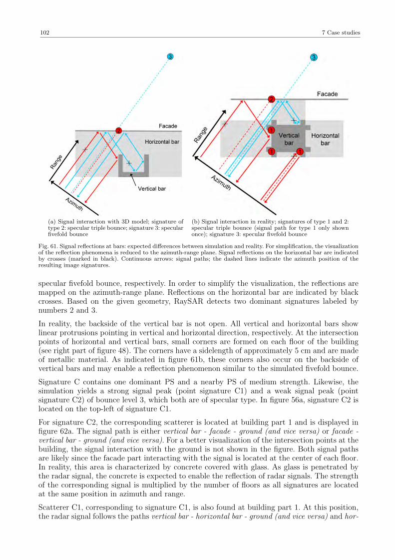
102 7 Case studies
(a) Signal interaction with 3D model; signature oftype 2: specular triple bounce; signature 3: specularfivefold bounce
(b) Signal interaction in reality; signatures of type 1 and 2:specular triple bounce (signal path for type 1 only shownonce); signature 3: specular fivefold bounce
Fig. 61. Signal reflections at bars: expected differences between simulation and reality. For simplification, the visualizationof the reflection phenomena is reduced to the azimuth-range plane. Signal reflections on the horizontal bar are indicatedby crosses (marked in black). Continuous arrows: signal paths; the dashed lines indicate the azimuth position of theresulting image signatures.
specular fivefold bounce, respectively. In order to simplify the visualization, the reflections aremapped on the azimuth-range plane. Reflections on the horizontal bar are indicated by blackcrosses. Based on the given geometry, RaySAR detects two dominant signatures labeled bynumbers 2 and 3.
In reality, the backside of the vertical bar is not open. All vertical and horizontal bars showlinear protrusions pointing in vertical and horizontal direction, respectively. At the intersectionpoints of horizontal and vertical bars, small corners are formed on each floor of the building(see right part of figure 48). The corners have a sidelength of approximately 5 cm and are madeof metallic material. As indicated in figure 61b, these corners also occur on the backside ofvertical bars and may enable a reflection phenomenon similar to the simulated fivefold bounce.
Signature C contains one dominant PS and a nearby PS of medium strength. Likewise, thesimulation yields a strong signal peak (point signature C1) and a weak signal peak (pointsignature C2) of bounce level 3, which both are of specular type. In figure 56a, signature C2 islocated on the top-left of signature C1.
For signature C2, the corresponding scatterer is located at building part 1 and is displayed infigure 62a. The signal path is either vertical bar - facade - ground (and vice versa) or facade -vertical bar - ground (and vice versa). For a better visualization of the intersection points at thebuilding, the signal interaction with the ground is not shown in the figure. Both signal pathsare likely since the facade part interacting with the signal is located at the center of each floor.In reality, this area is characterized by concrete covered with glass. As glass is penetrated bythe radar signal, the concrete is expected to enable the reflection of radar signals. The strengthof the corresponding signal is multiplied by the number of floors as all signatures are locatedat the same position in azimuth and range.
Scatterer C1, corresponding to signature C1, is also found at building part 1. At this position,the radar signal follows the paths vertical bar - horizontal bar - ground (and vice versa) and hor-
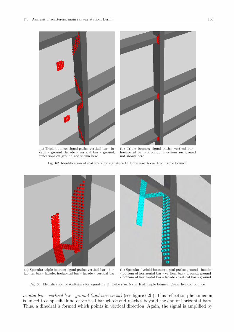
7.3 Analysis of scatterers: main railway station, Berlin 103
(a) Triple bounce; signal paths: vertical bar - fa-cade - ground; facade - vertical bar - ground;reflections on ground not shown here
(b) Triple bounce; signal paths: vertical bar -horizontal bar - ground; reflections on groundnot shown here
Fig. 62. Identification of scatterers for signature C. Cube size: 5 cm. Red: triple bounce.
(a) Specular triple bounce; signal paths: vertical bar - hor-izontal bar - facade; horizontal bar - facade - vertical bar
(b) Specular fivefold bounce; signal paths: ground - facade- bottom of horizontal bar - vertical bar - ground; ground- bottom of horizontal bar - facade - vertical bar - ground
Fig. 63. Identification of scatterers for signature D. Cube size: 5 cm. Red: triple bounce; Cyan: fivefold bounce.
izontal bar - vertical bar - ground (and vice versa) (see figure 62b). This reflection phenomenonis linked to a specific kind of vertical bar whose end reaches beyond the end of horizontal bars.Thus, a dihedral is formed which points in vertical direction. Again, the signal is amplified by
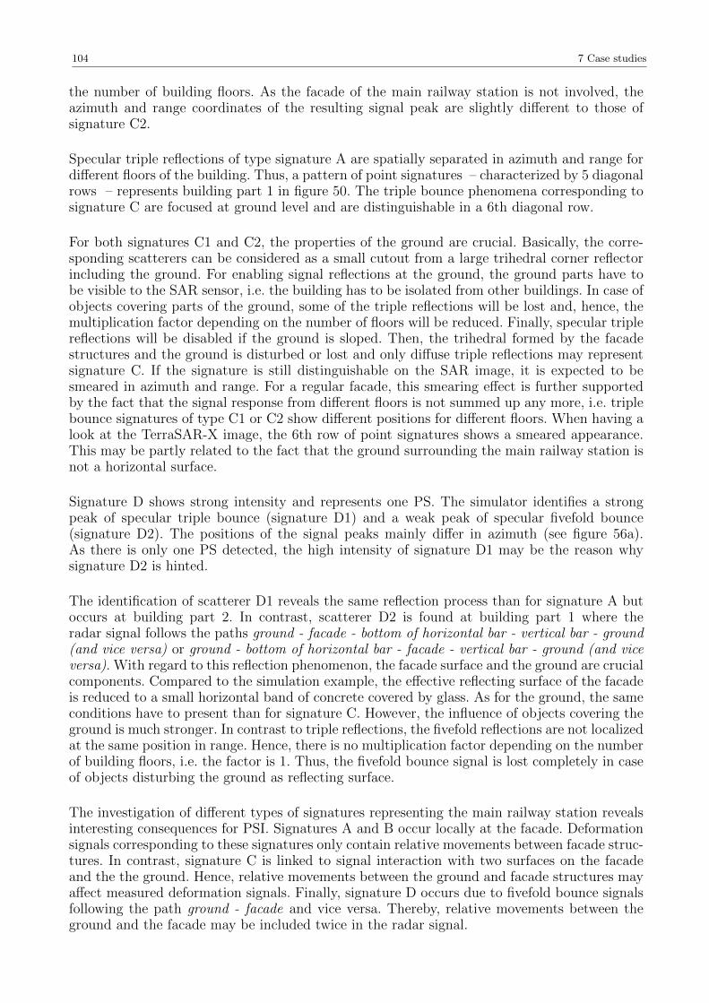
104 7 Case studies
the number of building floors. As the facade of the main railway station is not involved, theazimuth and range coordinates of the resulting signal peak are slightly different to those ofsignature C2.
Specular triple reflections of type signature A are spatially separated in azimuth and range fordifferent floors of the building. Thus, a pattern of point signatures – characterized by 5 diagonalrows – represents building part 1 in figure 50. The triple bounce phenomena corresponding tosignature C are focused at ground level and are distinguishable in a 6th diagonal row.
For both signatures C1 and C2, the properties of the ground are crucial. Basically, the corre-sponding scatterers can be considered as a small cutout from a large trihedral corner reflectorincluding the ground. For enabling signal reflections at the ground, the ground parts have tobe visible to the SAR sensor, i.e. the building has to be isolated from other buildings. In case ofobjects covering parts of the ground, some of the triple reflections will be lost and, hence, themultiplication factor depending on the number of floors will be reduced. Finally, specular triplereflections will be disabled if the ground is sloped. Then, the trihedral formed by the facadestructures and the ground is disturbed or lost and only diffuse triple reflections may representsignature C. If the signature is still distinguishable on the SAR image, it is expected to besmeared in azimuth and range. For a regular facade, this smearing effect is further supportedby the fact that the signal response from different floors is not summed up any more, i.e. triplebounce signatures of type C1 or C2 show different positions for different floors. When having alook at the TerraSAR-X image, the 6th row of point signatures shows a smeared appearance.This may be partly related to the fact that the ground surrounding the main railway station isnot a horizontal surface.
Signature D shows strong intensity and represents one PS. The simulator identifies a strongpeak of specular triple bounce (signature D1) and a weak peak of specular fivefold bounce(signature D2). The positions of the signal peaks mainly differ in azimuth (see figure 56a).As there is only one PS detected, the high intensity of signature D1 may be the reason whysignature D2 is hinted.
The identification of scatterer D1 reveals the same reflection process than for signature A butoccurs at building part 2. In contrast, scatterer D2 is found at building part 1 where theradar signal follows the paths ground - facade - bottom of horizontal bar - vertical bar - ground(and vice versa) or ground - bottom of horizontal bar - facade - vertical bar - ground (and viceversa). With regard to this reflection phenomenon, the facade surface and the ground are crucialcomponents. Compared to the simulation example, the effective reflecting surface of the facadeis reduced to a small horizontal band of concrete covered by glass. As for the ground, the sameconditions have to present than for signature C. However, the influence of objects covering theground is much stronger. In contrast to triple reflections, the fivefold reflections are not localizedat the same position in range. Hence, there is no multiplication factor depending on the numberof building floors, i.e. the factor is 1. Thus, the fivefold bounce signal is lost completely in caseof objects disturbing the ground as reflecting surface.
The investigation of different types of signatures representing the main railway station revealsinteresting consequences for PSI. Signatures A and B occur locally at the facade. Deformationsignals corresponding to these signatures only contain relative movements between facade struc-tures. In contrast, signature C is linked to signal interaction with two surfaces on the facadeand the the ground. Hence, relative movements between the ground and facade structures mayaffect measured deformation signals. Finally, signature D occurs due to fivefold bounce signalsfollowing the path ground - facade and vice versa. Thereby, relative movements between theground and the facade may be included twice in the radar signal.
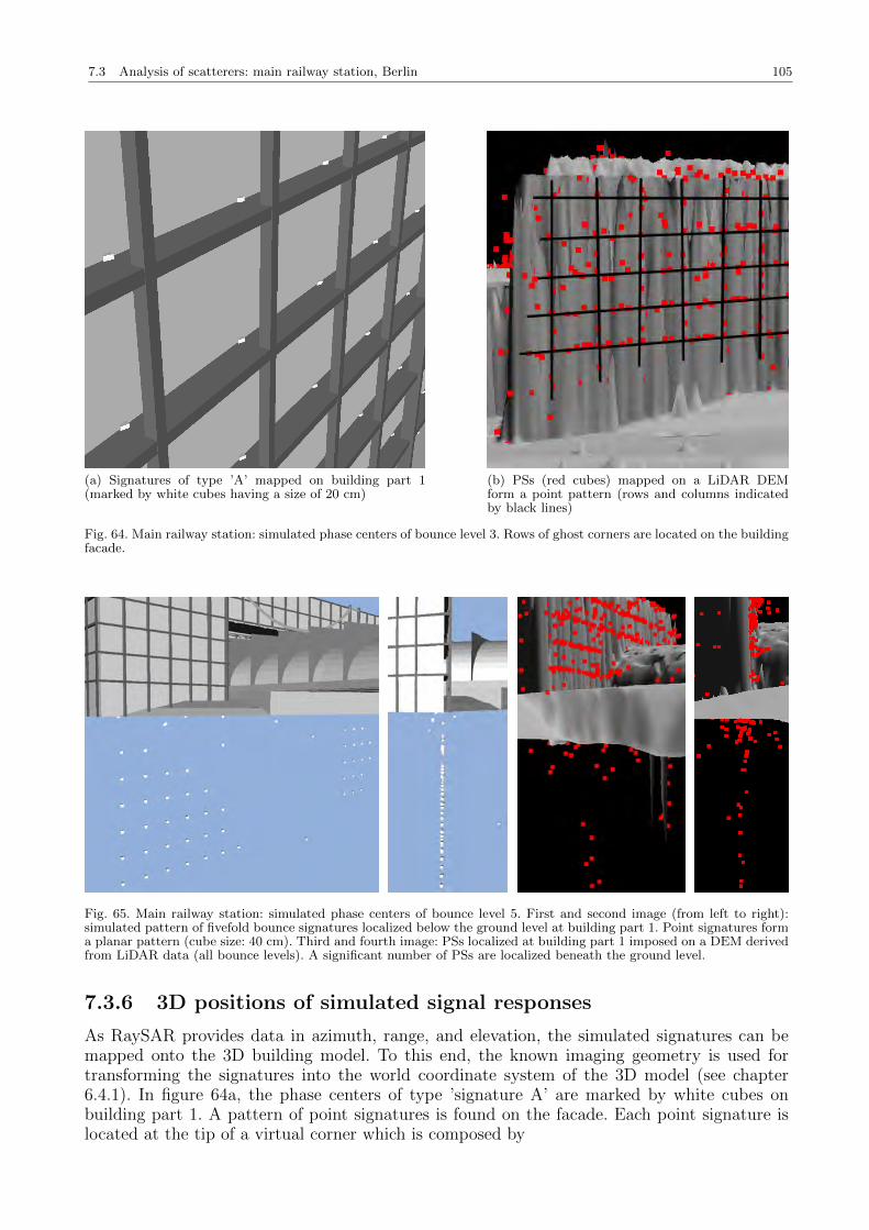
7.3 Analysis of scatterers: main railway station, Berlin 105
(a) Signatures of type ’A’ mapped on building part 1(marked by white cubes having a size of 20 cm)
(b) PSs (red cubes) mapped on a LiDAR DEMform a point pattern (rows and columns indicatedby black lines)
Fig. 64. Main railway station: simulated phase centers of bounce level 3. Rows of ghost corners are located on the buildingfacade.
Fig. 65. Main railway station: simulated phase centers of bounce level 5. First and second image (from left to right):simulated pattern of fivefold bounce signatures localized below the ground level at building part 1. Point signatures forma planar pattern (cube size: 40 cm). Third and fourth image: PSs localized at building part 1 imposed on a DEM derivedfrom LiDAR data (all bounce levels). A significant number of PSs are localized beneath the ground level.
7.3.6 3D positions of simulated signal responses
As RaySAR provides data in azimuth, range, and elevation, the simulated signatures can bemapped onto the 3D building model. To this end, the known imaging geometry is used fortransforming the signatures into the world coordinate system of the 3D model (see chapter6.4.1). In figure 64a, the phase centers of type ’signature A’ are marked by white cubes onbuilding part 1. A pattern of point signatures is found on the facade. Each point signature islocated at the tip of a virtual corner which is composed by
106 7 Case studies
one plane defined by the surface of a vertical bar, one plane defined by the surface of a horizontal bar, one plane defined by the facade of building part 1.
As the triple bounce signatures are not necessarily caused by physical corners, they representghost corners. Likewise, a point pattern of the same kind can also be found at building part 2.However, the number of point signatures is less in numbers than for building part 1 as the glassyroof in between building parts 1 and 2 reduces the effective height of the facade of building part2. In figure 64b, the localized PSs are mapped onto a LiDAR DEM of the main railway station.In contrast to figure 64a showing only triple bounce contributions, PSs of all bounce levels aredisplayed. As simulated by RaySAR, the point pattern on the facade is confirmed. Overall, thePS show little deviation from the horizontal and vertical lines colored in black which have beenintroduced artificially. A major factor influencing the deviation from the point pattern is thelimited accuracy of the localization in elevation due to the narrow orbital tube of TerraSAR-X.
When mapping the simulated fivefold bounce signatures of type ’D2’ into the 3D model, they arefound beneath the ground level at building part 1. On the left part of figure 65, two perspectiveviews onto the resulting point pattern are shown. As for the triple reflections, the signaturesare organized in a vertical point pattern. Since the signatures are linked to multiple reflectionsat horizonatal and vertical bars, the spatial distribution depends on the regularity of structureson the facade of building part 1.
Mapping the PSs onto the DEM reveals that some of the PSs are localized beneath buildingpart 1 and are approximately grouped on a vertical plane as well (right part of figure 65). Thepoints are less in numbers than in the simulated result and are irregularly distributed. Again,the deviation from the vertical plane is affected by the limited accuracy of the localizationin elevation. With regard to limitations of the simulated result, the ground is only roughlyapproximated as the ground level is represented by a flat plane in the 3D model. As indicatedby the LiDAR DEM, the real ground in front of the facade slightly varies in height and ispartly covered with objects. Hence, the majority of the simulated fivefold bounce signal isunlikely to occur since specular reflections are disturbed or made impossible. Nonetheless, theappearance of regular patterns of PSs below the ground level is confirmed for other isolatedbuildings in the center of Berlin. Hence, even if the difference between the simulation resultand the distribution of PSs is evident, a strong hint is given that also specular fivefold bouncesignatures are exploited as PSs.
8 Discussion and outlook 107
8 Discussion and outlook
In the introduction part of this thesis, three objectives are summarized which lead to researchconducted for the development and application of simulation methods. In the following, theresults of the thesis are discussed with reference to these objectives.
The first objective is to enable 3D SAR simulation using object models of high detail. Using aspecific imaging concept, that is an orthographic camera in combination with a source emittingparallel signals, this objective has been realized. The resulting SAR simulator is named RaySARand has been developed based on ray tracing methods. Signal contributions are simulated inazimuth, range, and elevation. Thereby, data are provided in SAR geometry and are used forproviding different simulation products, which can be compared to real SAR data. Reflectivitymaps in the azimuth-range plane support the visual interpretation of real data. Moreover, thesemaps are used for selecting pixels of interest whose correspondence to scatterers can be analyzed.For instance, elevation profiles can be defined in order to separate signal contributions in cross-range direction. By linking the simulated reflectivity maps to real SAR data, the inversion ofthe SAR imaging system can be simulated. Hence, in case of SAR image signatures confirmedby RaySAR, the interaction of radar signals with surfaces can be visualized in the simulated3D models.
The 3D position of signal contributions is derived directly without simulating the syntheticaperture. RaySAR represents an ideal SAR system which, for instance, focuses the signal re-sponse of a trihedral at one point in space. Only the peak position of signatures is simulatedwheras providing a copy of real SAR data is not persued. By direct simulation of the signalresponse from objects, calculating time is saved as no processing of raw data is required. Thus,simulation results for different imaging geometries or different object properties can be providedwithin minutes.
SAR simulation based on ray tracing reveals several limitations. First, the radiometrical cor-rectness of simulated signal responses is moderate. In order to improve the image radiometry,the reflection models of RaySAR may be exchanged with more reliable ones. However, only littleimprovement is expected, especially in case of multiple reflections. While specular reflectionsare covered by 100%, the representation of diffuse multiple reflections lacks of completenessconcerning both the geometry and the radiometry. For example, the ray tracer enables will notgeometrically describe 50 % of diffuse fourfold bounce signals occurring in a scene.
The reliability of the simulation results depends significantly on the level of detail of objectmodels. For VHR SAR data, theoretical assumptions indicate that the geometry of cornershaving a sidelength larger than 5 cm should be represented in 3D models. However, the avail-ability of those details in 3D models is only realistic for prominent objects. At present, basic citymodels are available in 2.5D or 3D where only basic facade details are geometrically described.To this end, different case studies have been conducted for discussing the influence of the levelof detail of object models:
Moderate level of detail: 3D models characterized by a low level of detail enable to sim-ulate the appearance of objects in the SAR image plane. Basic support is given for orientingin SAR data or for the visual interpretation of large image signatures. In most cases, dif-fuse reflection of Lambertian type has to be assigned to surfaces in order to guarantee thatobjects are distinguishable in the simulated data, e.g. object outlines or shadow areas. Theseparation of different reflection levels by means of image layers enables to provide a-prioriknowledge about objects. Signals of reflection level 1 describe object outlines in the SARimage plane which may be used, for instance, for grouping signatures representing singleobjects. The bottom lines of objects can be described by means of double bounce signatures.For 3D models of low detail, only large corners are simulated which may be used for linking
108 8 Discussion and outlook
simulated data and real SAR data. However, the low level of detail of the object modelslimits the directed analysis of signatures. Detailed 3D object models enable more realistic simulations as the geometry of small
object features is described. The major gain of information is observed for reflection levelshigher than 2. For instance, point patterns representing building facades in VHR SAR datacan be reproduced. In this context, the dependance of diffuse reflection on the directionof reflection can be confirmed. Then, the appearance of objects is likely to be reduced toa low number of signatures on the simulated image. Nonetheless, this will correspond tothe object appearance on the real SAR image if the surface parameters have been definedappropriately. Eventually, finding the link between simulated and real data becomes morerobust as the geometrical and radiometrical correctness of simulated signatures increases.
The second objective of the thesis is to enhance the knowledge about the nature of scatterers. Inorder to fulfil this task, several case studies have been conducted for single/multi body scenesas well as for object models characterized by different levels of detail. Still, the investigation ofreflection phenomena is in the early stages. However, a first insight into the nature of scatterersat buildings is enabled.
Double bounce: Linear signatures at building walls which are rotated with respect tothe line-of-sight of the SAR sensor require Lambertian-like diffuse signal reflection. In otherwords, the diffuse reflection of the radar signal has to be almost independent from the re-flection angle. The diffuse scatterer may be either the facade or the ground surrounding abuilding. In contast, the intensity of double bounce lines is expected to be weak if the diffusereflection depends on the reflection angle. Triple bounce: When being localized in 3D, the majority of signal contributions of reflection
level 3 are located either on facades or at the bottom of building walls. The first case occursdue to local triple bounce at features on the facade, e.g. windows or balconies. In contrast,the second case requires signal interaction with the ground surrounding the building and twosignal reflections on the building facade. At facades characterized by rows of windows, pointpatterns corresponding to specular triple bounce are the most prominent image signatures.When aiming at the simulation of those signatures, at least basic facade details have to begeometrically described in the 3D model. Reflection levels larger than 3: Two case studies – the Wynn hotel and the main railway
station – give strong hints that signals of reflection levels higher than 3 are apparent in VHRSAR data. Moreover, signatures of reflection level 5 are likely to be exploited as persistentscatterers. When localizing signal responses at buildings, e.g. by means of PSI, some of themwrongly found beneath the ground level. The simulation results for the main railway stationreveal that this pheomenon is likely to be related to multiple reflections. Specular fivefoldbounce is expected for isolated buildings surrounded by flat terrain which is covered, forinstance, by concrete or asphalt. In this case, the reliability of the position of simulatedfivefold bounce signatures also depends on the ground model. Hence, the ground has to bemodeled in detail, for instance, by using a high resolution DEM.
A high number of signatures lack of correspondance to features of the imaged object, i.e. theydo not represent the geometry of the scatterer. For instance, the majority of the point signaturesrepresenting the main railway station of Berlin fit into this category and, hence, may be labeledas ghost corners. Therefore, the extraction of object information based on multiple reflectedradar signals may lead to errors. This problem should be kept in mind since lines or pointsignatures are confirmed by the simulator as being prominent hints for urban objects.
The third objective of the thesis is to develop a SAR simulator based on existing software pack-ages. Parts of RaySAR are based on POV-Ray, an open-source raytracer. Own developmentshave been added to the source code in order to provide output data in SAR geometry. Using anexisting software has proven to be reasonable as the available methods are fast and reliable. Inaddition, using existing tools saved development time which could be used for working on the
8 Discussion and outlook 109
core of this thesis: the development of a 3D SAR simulator and the investigation of the originof SAR image signatures.
The current status of RaySAR offers several aspects for future work which mainly concern theenhancement of RaySAR and the analysis of reflection phenomena.
First, potentials for improving the SAR simulator have to be tested. In this regard, the focus maybe on increasing the completeness of diffuse multiple reflections. In its current form, RaySARdoes not enable to cover all relevant diffuse multiple reflections. Instead, only a small insight intodiffuse reflection phenomena is possible. However, concentrating on the simulation of multiplereflections including one diffuse reflection is reasonable. For instance, fourfold bounce signaturesrepresenting the Wynn Hotel may be explained in more detail (see chapter 7.2). As the raytracer is only a component of the RaySAR package, it can be exchanged with more sophisticatedrendering methods, which consider the exchange of diffuse signals between objects. Adding theradiosity algorithm (Goral et al., 1984) to basic ray tracing may be a way to solve this task.An alternative solution may be the application of path tracing (Kajiya, 1986) where rays arerandomly distributed at intersected surfaces. Nonethess, both methods will lead to a significantincrease of the calculating time which hampers the testing of different imaging geometries orthe simulation of SAR image stacks.
Second, the exploitation of VHR SAR data leads to the need of new simulation methods tobe added to RaySAR. For instance, 2D simulation methods may be applied or extended forproviding a-priori knowledge for object extraction or change detection using real SAR data. PSIprocessing may make use of grouping patterns of point signatures within the simulated outline ofurban objects. As shown in Gernhardt and Hinz (2008), the reliability of deformation estimationcan be increased when monitoring groups of scatterers. Simulating the outline of buildings orbuilding shadow may also support algorithms for change detection as image signatures canbe assigned to single objects of interest. New concepts for tomographic SAR may be tested bymeans of data stacks simulated for basic object models. To this end, the SAR imaging geometryand phase noise of real SAR missions can be considered.
Finally, the developed methods for 3D analysis enable further case studies on the nature ofscatterers. Especially, a categorization of ghost corners is reasonable. This can be seen for themain railway station of Berlin (see chapter 7.3.6). Ghost corners on the building facade lackof correspondence to metallic bars but describe the main corpus of the building. In contrast,triple bounce signals located on the ground or fivefold bounce signals found beneath the groundlevel do not represent the geometry of the building. The simulation of highly detailed modelsmay enable to recover new reflection phenomena. Unfortunately, 3D models of high detail areonly available for prominent buildings. Hence, in most cases, reflection phenomena will haveto be explained by means of 3D models describing the main features of objects. This may besufficient as, for instance, the simulation of the University of Stuttgart reveals that prominentimage signatures representing a building can be confirmed when considering basic facade details.
110 A Radar reflection models
A Radar reflection models
Specular reflections of radar signals are commonly described by the Fresnel reflection model. Fordiffuse reflections, different reflection models such as the Small Perturbation Method (SPM)or the Kirchhoff Approach (KA) have been defined for different levels of surface roughness.In the following, the Fresnel reflection model and the SPM are briefly recapitulated. Detailedinformation can be found, for instance, in Franceschetti et al. (2001) and Tsang and Kong(2001).
Fresnel reflection model
The Fresnel reflection coefficients, providing the portion of signal reflected in specular direction,depend on the angle of incidence of the incoming signal θi as well as on the complex relativedielectric constant defined as
εr =ε2
ε1
(A.1)
describing the proportion between the permittivity of the upper medium and lower mediumin a simulated scene. In the SAR simulation case, the upper and lower medium represent theatmosphere and a reflecting surface at the earth surface, respectively. The Fresnel coefficient inhorizontal polarization is calculated by
rh =
∣∣∣∣∣∣cos θi −√εr − sin2 θi
cos θi +√εr − sin2 θi
∣∣∣∣∣∣2
(A.2)
and the Fresnel coefficient in vertical polarization is defined as
rv =
∣∣∣∣∣∣εr cos θi −√εr − sin2 θi
εr cos θi +√εr − sin2 θi
∣∣∣∣∣∣2
(A.3)
Small Perturbation Method (SPM)
The Small Perturbation Method (SPM) approximates the diffuse reflection of radar signals atsurfaces whose surface height variation is small compared to the signal wavelength. From thegeometrical point of view, the strength of diffuse reflected signals depends on three angles: theangle of incidence θi of the incoming signal and two angles defining the direction of reflection,i.e. θr representing the reflection angle with respect to the surface normal and ϑr defining therotation with respect to the incident field. The power density of a signal diffusely reflected intoa certain direction is derived by
|Epq|2 =4a |k2 cos θr cos θiβpq|2W (ηxy)
(2πR)2 (A.4)
where a is the area of the surface, k = 2πλ
is the signal wavenumber, and R is the spatial distancebetween SAR and object. W (κx, κy) is the surface power spectrum, i.e. the Fourier transformof the surface autocorrelation function. It may be defined by means of standard surface modelssuch as gaussian or exponential shapes or by using fractals (Franceschetti et al., 2001). In this
A Radar reflection models 111
thesis, an isotropic gaussian surface was used for surface representation, which may be definedas
W (κx, κy) = πσ2L2c · exp
−√κ2x + κ2
y · Lc2
2 (A.5)
where σ is the surface standard deviation and Lc is the surface correlation length. Finally, signalpolarimetry is considered by parameter βpq. At this point, the examples of HH and V V areintroduced:
βhh =(εr − 1) cos (ϑr)(
cos θr +√εr − sin2 θr
)·(
cos θi +√εr − sin2 θi
) (A.6)
βvv =
(√εr − sin2 (θr) ·
√εr − sin2 (θi) · cosϑr − εr sin (θi) sin (θr)
)· (εr − 1)(
εr cos θr +√εr − sin2 θr
)·(εr cos θi +
√εr − sin2 θi
) (A.7)
The parameters for cross-polarization can be found in Franceschetti et al. (2001).
112 B POV-Ray: Introduction and Modeling
B POV-Ray: Introduction and Modeling
B.1 Introduction to POV-Ray
The idea for POV-Ray (POV-Ray, 2011), where the abbrevation POV stands for Persistenceof Vision, was born in May 1991 when David Buck offered the development of a new raytracer to the render community. POV-Ray should be based on DKB-Trace, an existing raytracer developed by Buck for Amiga graphics which had been adapted to be used on personalcomputers (Buck, 2011). Since then, POV-Ray has been enhanced and has currently reachedversion 3.6.2. It is an open-source software programmed in C++ where own developments can beadded to its source-code. Ray tracing, radiosity and a simplified version of photon mapping aresupported. Modeling is performed in a text editor for defining scene objects and render settings.To this end, POV-Ray owns a programming language which is translated by a parser for beingused in the C++ source code. In addition, modeling software is available for providing POV-Rayscenes, e.g. Moray (Moray, 2011) or Wings3D (Wings3D, 2011). Transforming standard modelformats in to the POV-Ray format (.pov) is possible, e.g. by using AccuTrans 3D (AccuTrans,2011). Further information about POV-Ray can be found, for instance, in Wolfe (1999) andin Lama (2004). Basics with regard to modeling in the POV-Ray editor are introduced in thenext subsection.
B.2 Modeling in the POV-Ray editor
Modeling in the POV-Ray editor is introduced from two aspects. First, tools for describing thescene geometry are presented. Afterward, parameters for defining the reflection characteristicsof objects are explained. In this context, the focus is on tools and parameters relevant for SARsimulation.
Scene geometry
Basically, a scene to be rendered has to contain three kinds of elements: at least one lightsource, a camera for defining the observer’s point of view and the geometry and material ofobjects. The standard light source is point light whose origin is situated at one point in space.The emission of parallel light is obtained using the POV-Ray command parallel. For instance,the properties of a light source emitting parallel light can be defined by
light sourcecolor rgb < I1, I2, I3 > parallel translate < x1, y1, z1 > point at < x2, y2, z2 >
The command color rgb < I1, I2, I3 > represents the emitted signal by one channel for blue,green, and red light, respectively. Furthermore, the position of the light source and the directionof the emitted signal are defined by vectors translate < x1, y1, z1 > and point at < x2, y2, z2 >,respectively.
Various camera types are offered by POV-Ray. A perspective camera, which is the standardcamera type, is defined by means of a projection center and an image plane, located in front ofthe projection center. Rays for detecting intensities in the 3D scene are defined by connectingthe projection center and the center of pixels on the image plane. The number of rays dependson the number of pixels on the image plane. The parallelism of rays is obtained by using anorthographic camera. In contrast to a perspective camera, the sampling density at objects isindependent from the spatial distance sensor-object and, hence, only depends on the spatial
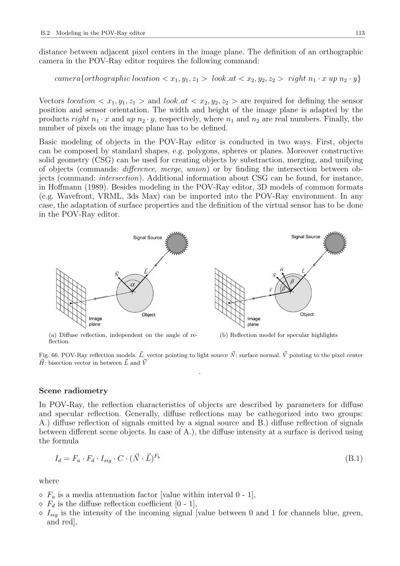
B.2 Modeling in the POV-Ray editor 113
distance between adjacent pixel centers in the image plane. The definition of an orthographiccamera in the POV-Ray editor requires the following command:
cameraorthographic location < x1, y1, z1 > look at < x2, y2, z2 > right n1 · x up n2 · y
Vectors location < x1, y1, z1 > and look at < x2, y2, z2 > are required for defining the sensorposition and sensor orientation. The width and height of the image plane is adapted by theproducts right n1 · x and up n2 · y, respectively, where n1 and n2 are real numbers. Finally, thenumber of pixels on the image plane has to be defined.
Basic modeling of objects in the POV-Ray editor is conducted in two ways. First, objectscan be composed by standard shapes, e.g. polygons, spheres or planes. Moreover constructivesolid geometry (CSG) can be used for creating objects by substraction, merging, and unifyingof objects (commands: difference, merge, union) or by finding the intersection between ob-jects (command: intersection). Additional information about CSG can be found, for instance,in Hoffmann (1989). Besides modeling in the POV-Ray editor, 3D models of common formats(e.g. Wavefront, VRML, 3ds Max) can be imported into the POV-Ray environment. In anycase, the adaptation of surface properties and the definition of the virtual sensor has to be donein the POV-Ray editor.
(a) Diffuse reflection, independent on the angle of re-flection.
(b) Reflection model for specular highlights
Fig. 66. POV-Ray reflection models. ~L: vector pointing to light source ~N : surface normal. ~V pointing to the pixel center~H: bisection vector in between ~L and ~V
.
Scene radiometry
In POV-Ray, the reflection characteristics of objects are described by parameters for diffuseand specular reflection. Generally, diffuse reflections may be cathegorized into two groups:A.) diffuse reflection of signals emitted by a signal source and B.) diffuse reflection of signalsbetween different scene objects. In case of A.), the diffuse intensity at a surface is derived usingthe formula
Id = Fa · Fd · Isig · C · ( ~N · ~L)Fb (B.1)
where
Fa is a media attenuation factor [value within interval 0 - 1], Fd is the diffuse reflection coefficient [0 - 1], Isig is the intensity of the incoming signal [value between 0 and 1 for channels blue, green,
and red],
114 B POV-Ray: Introduction and Modeling
C is the color of the surface hit by the signal [value between 0 and 1 for channels blue, green,and red],
~N is the surface normal vector, ~L is the normalized signal vector pointing from the surface point to the signal source, and Fb is a surface brilliance factor.
According to equation B.1, diffuse reflection at object surfaces is assumed to be of type ’lam-bertian’. Figure 66a displays a diffuse reflection process. The reflected intensity only dependon the incidence angle α of the incoming signal hitting the surface. Diffuse signal reflectionsbetween objects, which corresponds to case B.), are not considered by the raytracing conceptand may only be represented by constant intensity (POV-Ray command ambient).
Specular highlights are added artificially in case of a specific geometry defined by the incomingray and the reflected ray. As shown in figure 66b, surface normal ~N and signal vector ~L, bothfixed at the intersection point detected by the ray tracer, define bisection vector ~H. In case ofspecular reflection, the angle between vectors ~N and ~H equals zero. The corresponding equationfor specular highlights is defined as
Is = Fs · C · ( ~N · ~H)1Fr (B.2)
where Fs is a specular reflection coefficient [0 - 1] and Fr is a roughness factor defining thesharpness of the specular highlight. In sum, the surface characteristics of an object may bedefined by using the command
texture pigment color rgb < I1, I2, I3 >finish reflection Fw diffuse Fd specular Fs roughness Fr
The color of the surface is defined by command pigment ·, while surface reflection is modeledby command finish ·. Command reflection · is required for weighting specular reflectedrays by factor Fw chosen from the interval between 0 and 1. In case of multiple reflections, raytracing is stopped if the ray’s weight falls below a given threshold, if the pre-defined trace levelmaximum is reached, or if no further intersection point is detected within the modeled scene.
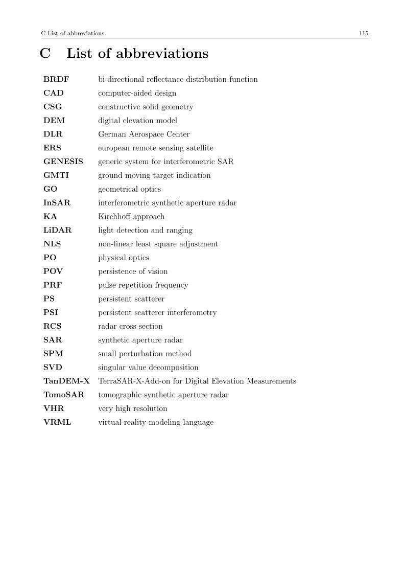
C List of abbreviations 115
C List of abbreviations
BRDF bi-directional reflectance distribution function
CAD computer-aided design
CSG constructive solid geometry
DEM digital elevation model
DLR German Aerospace Center
ERS european remote sensing satellite
GENESIS generic system for interferometric SAR
GMTI ground moving target indication
GO geometrical optics
InSAR interferometric synthetic aperture radar
KA Kirchhoff approach
LiDAR light detection and ranging
NLS non-linear least square adjustment
PO physical optics
POV persistence of vision
PRF pulse repetition frequency
PS persistent scatterer
PSI persistent scatterer interferometry
RCS radar cross section
SAR synthetic aperture radar
SPM small perturbation method
SVD singular value decomposition
TanDEM-X TerraSAR-X-Add-on for Digital Elevation Measurements
TomoSAR tomographic synthetic aperture radar
VHR very high resolution
VRML virtual reality modeling language
116 REFERENCES
References
AccuTrans, 2011. AccuTrans 3D. Micromouse Productions, www.micromouse.ca [checked: 24.02.2011].Adam, N., Eineder, M., Yague-Martinez, N., Bamler, R., 2008. High resolution interferometric stacking
with TerraSAR-X. In: Proceedings of IEEE International Geoscience and Remote Sensing Sympo-sium (IGARSS), Vol. 2, 117–120.
Adam, N., Zhu, X., Minet, C., Liebhart, W., Eineder, M., Bamler, R., 2009. Techniques and examplesfor the 3D reconstruction of complex scattering situations using TerraSAR-X. In: Proceedings ofIEEE International Geoscience and Remote Sensing Symposium (IGARSS), Vol. 3, 900–903.
Appel, A., 1968. Some techniques for shading machine renderings of solids. In: Proceedings of thespring joint computer conference AFIPS, ACM, New York, NY, USA, 37–45.
Attema, E., Duchossois, G., Kohlhammer, G., 1998. ERS-1/2 SAR land applications: overview andmain results. In: Proceedings of IEEE International Geoscience and Remote Sensing Symposium(IGARSS), Vol. 4, 1796–1798.
Auer, S., Balz, T., Becker, S., Bamler, R., 2010a. 3D SAR simulation of urban areas based on detailedbuilding models. Photogrammetric Engineering & Remote Sensing, Journal of the American Societyfor Photogrammetry and Remote Sensing 76 (12): 1373–1384.
Auer, S., Hinz, S., Bamler, R., 2008. Ray tracing for simulating reflection phenomena in SAR images.In: Proceedings of IEEE International Geoscience and Remote Sensing Symposium (IGARSS),Vol. 5, 518–521.
Auer, S., Hinz, S., Bamler, R., 2010b. Ray-tracing simulation techniques for understanding high-resolution SAR images. IEEE Transactions on Geoscience and Remote Sensing 48 (3): 1445–1456.
Auer, S., Zhu, X., Hinz, S., Bamler, R., 2009a. 3D analysis of scattering effects based on ray tracingtechniques. In: Proceedings of IEEE International Geoscience and Remote Sensing Symposium(IGARSS), Vol. 3, 17–20.
Auer, S., Zhu, X., Hinz, S., Bamler, R., 2009b. Ray tracing and SAR-tomography for 3D analysis ofmicrowave scattering at man-made objects. In: International Archives of Photogrammetry, RemoteSensing and Spatial Information Sciences, Vol. 38-3/W4, 157–162.
Balz, T., 2006. Real-time SAR simulation of complex scenes using programmable graphics processingunits. In: Proceedings of the ISPRS TCVII Mid-term Symposium, Enschede.
Balz, T., Stilla, U., 2009. Hybrid GPU-based single- and double-bounce SAR simulation. IEEE Trans-actions on Geoscience and Remote Sensing 47: 3519–3529.
Bamler, R., 1992. A comparison of range-doppler and wavenumber domain SAR focusing algorithms.IEEE Transactions on Geoscience and Remote Sensing 30 (4): 706–713.
Bamler, R., Eineder, M., 2008. The pyramids of gizeh seen by TerraSAR-X - a prime example forunexpected scattering mechanisms in SAR. IEEE Geoscience and Remote Sensing Letters 5 (3):468–470.
Bamler, R., Hartl, P., 1998. Synthetic aperture radar interferometry. Inverse Problems 14: R1–R54.Becker, S., 2009. Generation and application of rules for quality dependent facade reconstruction.
ISPRS Journal of Photogrammetry and Remote Sensing 64 (6): 640–653.Berges, A., Latger, J., Mametsa, H., 2004. FERMAT a new radar simulation approach. In: Proceedings
of International Conference on Radar Systems (RADAR).Bickert, B., Meyer-Hilberg, J., Schmid, J., 2002. A radar raw data generator and modular algorithm
simulation system for MTI development. In: Proceedings of the European Conference on SyntheticAperture Radar (EUSAR).
Bolter, R., 2001. Buildings from SAR: Detection and reconstruction of buildings from multiple viewhigh resolution SAR data. Ph.D. thesis, Technische Universitat Graz, Graz.
Bolter, R., Leberl, F., 2000. Detection and reconstruction of buildings from multiple view interferomet-ric SAR data. In: Proceedings of IEEE International Geoscience and Remote Sensing Symposium(IGARSS), Vol. 2, 749–751.
Bouknight, W., 1970. A procedure for generation of three-dimensional half-toned computer graphicspresentations. Commun. ACM 13 (9): 527–536.
REFERENCES 117
Boyell, R., 1969. Computer simulation of lunar displays. In: Proceedings of SPIE Conference, Vol. 2,339–356.
Breit, H., Fritz, T., Balss, U., Lachaise, M., Niedermeier, A., Vonavka, M., 2010. TerraSAR-X SARprocessing and products. IEEE Transactions on Geoscience and Remote Sensing 48 (2): 727–740.
Brunner, D., 2009. Advanced methods for building information extraction from very high resolutionSAR data to support emergency response. Ph.D. thesis, University of Trento.
Brunner, D., Bruzzone, L., Ferro, A., Lemoine, G., 2009. Analysis of the reliability of the double bouncescattering mechanism for detecting buildings in VHR SAR images. In: Proceedings of RadarCon2009, Pasadena, USA.
Buck, D., 2011. The early history of POV-Ray. www.povray.org [checked: 24.02.2011].Budillon, A., Evangelista, A., Schirinzi, G., 2009. SAR tomography from sparse samples. In: Proceed-
ings of IEEE International Geoscience and Remote Sensing Symposium (IGARSS), Vol. 4, IV–865–IV–868.
Camporeale, C., Galati, G., 1991. Digital computer simulation of synthetic aperture systems andimages. European Transactions on Telecommunications 2 (NO: 3): 343–352.
Catmull, E., 1974. A subdivision algorithm for computer display of curved surfaces. Ph.D. thesis,University of Utah.
Cook, R. L., Porter, T., Carpenter, L., 1984. Distributed ray tracing. SIGGRAPH Comput. Graph.18 (3): 137–145.
Cumming, I., Wong, F., 2005. Digital Processing of Synthetic Aperture Radar Data: Algorithms andImplementation. Artech House Publishers.
Eiffel, 2011. Le site officiel de la tour eiffel. www.tour-eiffel.fr [checked: 24.02.2011].Eineder, M., 2003. Efficient simulation of SAR interferograms of large areas and of rugged terrain.
IEEE Transactions on Geoscience and Remote Sensing 41 (6): 1415–1427.Eineder, M., Adam, N., Bamler, R., Yague-Martinez, N., Breit, H., 2009. Spaceborne spotlight SAR
interferometry with TerraSAR-X. IEEE Transactions on Geoscience and Remote Sensing 47 (5):1524–1535.
Eineder, M., Adam, N., Brcic, R., Yague-Martinez, N., Fritz, T., 2008. High bandwidth spotlight SARinterferometry with TerraSAR-X. In: Proceedings of IEEE International Geoscience and RemoteSensing Symposium (IGARSS) 2008, Vol. 2, 113–116.
Ferretti, A., Bianchi, M., Prati, C., Rocca, F., 2005. Higher-order permanent scatterers analysis.EURASIP J. Appl. Signal Process. : 3231–3242.
Ferretti, A., Prati, C., Rocca, F., 2001. Permanent scatterers in SAR interferometry. IEEE Transac-tions on Geoscience and Remote Sensing 39 (1): 8–20.
Fornaro, G., Reale, D., Serafino, F., 2009. Four-dimensional SAR imaging for height estimation andmonitoring of single and double scatterers. IEEE Transactions on Geoscience and Remote Sensing47 (1): 224–237.
Fornaro, G., Serafino, F., Soldovieri, F., 2003. Three-dimensional focusing with multipass SAR data.IEEE Transactions on Geoscience and Remote Sensing 41 (3): 507–517.
Franceschetti, G., Guida, R., Iodice, A., Riccio, D., Ruello, G., Stilla, U., 2007. Building feature extrac-tion via a deterministic approach: application to real high resolution SAR images. In: Proceedingsof IEEE International Geoscience and Remote Sensing Symposium (IGARSS), 2681–2684.
Franceschetti, G., Iodice, A., Migliaccio, M., Riccio, D., 1998. A novel across-track SAR interferometrysimulator. IEEE Transactions on Geoscience and Remote Sensing 36 (3): 950 –962.
Franceschetti, G., Iodice, A., Riccio, D., 2001. Fractal Models for Scattering from Natural Surfaces.Academic Press, Ch. 1.6.5, 467–485.
Franceschetti, G., Iodice, A., Riccio, D., 2002. A canonical problem in electromagnetic backscatteringfrom buildings. IEEE Transactions on Geoscience and Remote Sensing 40 (8): 1787–1801.
Franceschetti, G., Iodice, A., Riccio, D., Ruello, G., 2003. SAR raw signal simulation for urban struc-tures. IEEE Transactions on Geoscience and Remote Sensing 41 (9): 1986–1995.
Franceschetti, G., Lanari, R., 1999. Synthetic Aperture Radar Processing. CRC Press LLC.Franceschetti, G., Migliaccio, M., Riccio, D., 1995. The SAR simulation: an overview. In: Proceedings
118 REFERENCES
of IEEE International Geoscience and Remote Sensing Symposium (IGARSS), Vol. 3, 2283–2285.Franceschetti, G., Migliaccio, M., Riccio, D., Schirinzi, G., 1992. SARAS: a synthetic aperture radar
(SAR) raw signal simulator. IEEE Transactions on Geoscience and Remote Sensing 30 (1): 110–123.Gamba, P., Houshmand, B., Saccani, M., 2000. Detection and extraction of buildings from interfero-
metric SAR data. IEEE Transactions on Geoscience and Remote Sensing 38 (1): 611–617.Gelautz, M., Frick, H., Raggam, J., Burgstaller, J., Leberl, F., 1998. SAR image simulation and analysis
of alpine terrain. ISPRS Journal of Photogrammetry and Remote Sensing 53 (1): 17–38.Gernhardt, S., Adam, N., Eineder, M., Bamler, R., 2010. Potential of very high resolution SAR for
persistent scatterer interferometry in urban areas. Annals of GIS 16 (2): 103–111.Gernhardt, S., Hinz, S., 2008. Advanced displacement estimation for PSI using high resolution SAR
data. In: Proceedings of IEEE International Geoscience and Remote Sensing Symposium (IGARSS),Vol. 3, 1276–1279.
Glassner, A. S., 2002. An Introduction to Ray Tracing, 9th Edition. Morgan Kaufmann, San Francisco.Goel, K., Adam, N., 2010. A bayesian method for very high resolution multi aspect angle radargram-
metry. In: Proceedings of the European Conference on Synthetic Aperture Radar (EUSAR).Google, 2011. Google 3D warehouse. http://sketchup.google.com/3dwarehouse [checked: 24.02.2011].Goral, C. M., Torrance, K. E., Greenberg, D. P., Battaile, B., 1984. Modeling the interaction of light
between diffuse surfaces. SIGGRAPH Comput. Graph. 18 (3): 213–222.Groot, J., Otten, M., 1993. Corner reflector imaging by high resolution SAR. In: Proceedings of SAR
Calibration Workshop ESA WPP-048, ESTEC, Noordwijk, The Netherlands, 43–50.Guida, R., Iodice, A., Riccio, D., 2010. Assessment of TerraSAR-X products with a new feature ex-
traction application: Monitoring of cylindrical tanks. IEEE Transactions on Geoscience and RemoteSensing 48 (2): 930–938.
Hammer, H., Balz, T., Cadario, E., Soergel, U., Thoennessen, U., Stilla, U., 2008. Comparison of SARsimulation concepts for the analysis of high resolution SAR data. In: Proceedings of the EuropeanConference on Synthetic Aperture Radar (EUSAR).
Hanssen, R., 2001. Radar Interferometry: Data Interpretation and Error Analysis, 1st Edition. KluwerAcademic Publishers, Dordrecht, The Netherlands.
Heckbert, P. S., Hanrahan, P., 1984. Beam tracing polygonal objects. In: SIGGRAPH ’84: Proceedingsof the 11th annual conference on Computer graphics and interactive techniques, ACM, New York,NY, USA, 119–127.
Henderson, F., Lewis, A., 1998. Principles & Applications of Imaging Radar. John Wiley & Sons, Inc.,New York.
Hill, R., Moate, C., Blacknell, D., 2006. Urban scene analysis from SAR image sequences. In: Proceed-ings of the European Conference on Synthetic Aperture Radar (EUSAR).
Hoffmann, C. M., 1989. Geometric & Solid Modeling. Morgan Kaufmann Publishers, San Mateo,California.
Holtzman, J., Frost, V., Abbott, J., Kaupp, V., 1978. Radar image simulation. IEEE Transactions onGeoscience Electronics 16 (4): 296–303.
Ikegami, F., Takeuchi, T., Yoshida, S., 1991. Theoretical prediction of mean field strength for urbanmobile radio. IEEE Transactions on Antennas and Propagation 39 (3): 299–302.
Jensen, H. W., 1996. Global illumination using photon maps. In: Proceedings of the eurographicsworkshop on Rendering techniques ’96, Springer-Verlag, London, UK, 21–30.
Kajiya, J. T., 1986. The rendering equation. SIGGRAPH Comput. Graph. 20 (4): 143–150.Kampes, B., 2006. Radar Interferometry - Persistent Scatterer Technique. Springer, Dordrecht, The
Netherlands.Knott, E., Shaeffer, J., Tuley, M., 2004. Radar Cross Section, 2nd Edition. SciTech Publishing, NC.Krieger, G., Moreira, A., Fiedler, H., Hajnsek, I., Werner, M., Younis, M., Zink, M., 2007. TanDEM-X:
A satellite formation for high-resolution SAR interferometry. IEEE Transactions on Geoscience andRemote Sensing 45 (11): 3317–3341.
Lama, T., 2004. 3D-Welten. Hanser, Munchen.LaPrade, G. L., 1963. An analytical and experimental study of stereo for radar. Photogrammetric
REFERENCES 119
Engineering 29 (2): 294–300.Latger, J., Mametsa, H., Berges, A., 2005. SPECRAY EM / FERMAT - a new modelling radar ap-
proach from numerical models of terrain to SAR images. In: Proceedings of International Conferenceon Radar Systems (RADAR).
Leberl, F., 1990. Radargrammetric Image Processing. Artech House, Boston, MA.Lehnert, H., 1993. Systematic errors of the ray-tracing algorithm. Applied Acoustics 38 (2-4): 207–221.Lichti, D., 2004. A resolution measure for terrestrial laser scanners. International Archives of Pho-
togrammetry, Remote Sensing and Spatial Information Sciences 34 34 (B5): 552–558.Lombardini, F., 2005. Differential tomography: a new framework for SAR interferometry. IEEE Trans-
actions on Geoscience and Remote Sensing 43 (1): 37–44.Lombardini, F., Reigber, A., 2003. Adaptive spectral estimation for multibaseline SAR tomography
with airborne L-band data. In: Proceedings of IEEE International Geoscience and Remote SensingSymposium (IGARSS), Vol. 3, 2014–2016.
Lombardo, P., 2004. A multichannel spaceborne radar for the COSMO-SkyMed satellite constellation.In: Proceedings of IEEE Aerospace Conference, Vol. 1, 111–119.
Louet, J., Bruzzi, S., 1999. ENVISAT mission and system. In: Proceedings of IEEE InternationalGeoscience and Remote Sensing Symposium (IGARSS), Vol. 3, 1680 –1682.
Mametsa, H. J., Rouas, F., Berges, A., Latger, J., 2001. Imaging radar simulation in realistic environ-ment using shooting and bouncing rays technique. In: Proceedings of SPIE Conference, SAR ImageAnalysis, Modeling and Techniques IV, 34–40.
Margarit, G., Mallorqui, J., Fortuny-Guasch, J., Lopez-Martinez, C., 2009. Phenomenological vesselscattering study based on simulated inverse SAR imagery. IEEE Transactions on Geoscience andRemote Sensing 47 (4): 1212–1223.
Margarit, G., Mallorqui, J. J., Lopez-Martinez, C., 2007. GRECOSAR, a SAR simulator for complextargets: Application to urban environments. In: Proceedings of IEEE International Geoscience andRemote Sensing Symposium (IGARSS), 4160–4163.
Margarit, G., Mallorqui, J. J., Rius, J. M., Sanz-Marcos, J., 2006. On the usage of GRECOSAR,an orbital polarimetric SAR simulator of complex targets, to vessel classification studies. IEEETransactions on Geoscience and Remote Sensing 44 (12): 3517–3526.
Melody, J., 2009. Predicted-wavefront backprojection for knowledge-aided SAR image reconstruction.In: Proceedings of RadarCon 2009, Pasadena, USA.
Meyer-Hilberg, J., 2006. PIRDIS: A new versatile tool for SAR/MTI systems simulation. In: Proceed-ings of the European Conference on Synthetic Aperture Radar (EUSAR).
Meyer-Hilberg, J., Neumann, C., Senkowski, H., 2008. GMTI systems simulation using the SAR sim-ulation tool PIRDIS. In: Proceedings of the European Conference on Synthetic Aperture Radar(EUSAR).
Michaelsen, E., Soergel, U., Stilla, U., 2002. Grouping salient scatterers in InSAR data for recognitionof industrial buildings. In: Proceedings of 16th International Conference on Pattern Recognition,Vol. 2, 613–616.
Moray, 2011. Moray. www.stmuc.com/moray [checked: 24.02.2011].Mori, A., De Vita, F., 2004. A time-domain raw signal simulator for interferometric SAR. IEEE
Transactions on Geoscience and Remote Sensing 42 (9): 1811–1817.Muhleman, D., 1964. Radar scattering from venus and the moon. Symposium on Radar and Radio-
metric Observations of Venus during the 1962 Conjunction 69: 34–41.Nasr, J., Vidal-Madjar, D., 1991. Image simulation of geometric targets for spaceborne synthetic
aperture radar. IEEE Transactions on Geoscience and Remote Sensing 29 (6): 986–996.Nicodemus, F., 1965. Directional reflectance and emissivity of an opaque surface. Appl. Opt. 4 (7):
767–773.Oriot, H., Cantalloube, H., 2008. Circular SAR imagery for urban remote sensing. In: Proceedings of
the European Conference on Synthetic Aperture Radar (EUSAR).Perski, Z., Van Leijen, F., Hanssen, R., 2007. Applicability of PSInSAR for building hazard identifi-
cation. study of the 29 January 2006 Katowice Exhibition Hall collapse and the 24 February 2006
120 REFERENCES
Moskow Basmanny Market collapse. In: Proceedings of the Envisat Symposium.Petit, D., Adragna, F., 2000. A new interferogram simulator: 2SIR. study of coherence losses for
tortured reliefs. In: Proceedings of SAR Workshop: CEOS - Working Group on Calibration andValidation, Vol. 450, 591–596.
Phong, B., 1975. Illumination for computer generated pictures. Communications of the ACM 18 18 (6):311–317.
Pitz, W., Miller, D., 2010. The TerraSAR-X satellite. IEEE Transactions on Geoscience and RemoteSensing 48 (2): 615–622.
POV-Ray, 2011. POV-Ray. Persistence of Vision Raytracer Propriety Limited, www.povray.org[checked: 24.02.2011].
Quartulli, M., Datcu, M., 2004. Stochastic geometrical modeling for built-up area understanding froma single SAR intensity image with meter resolution. IEEE Transactions on Geoscience and RemoteSensing 42 (9): 1996–2003.
Raney, R., Wessels, G., 1988. Spatial considerations in SAR speckle consideration. IEEE Transactionson Geoscience and Remote Sensing 26 (5): 666–672.
Reigber, A., Moreira, A., 2000. First demonstration of airborne SAR tomography using multibaselineL-band data. IEEE Transactions on Geoscience and Remote Sensing 38 (5): 2142–2152.
Rius, J., Ferrando, M., Jofre, L., 1993. GRECO: graphical electromagnetic computing for RCS pre-diction in real time. IEEE Antennas and Propagation Magazine 35 (2): 7–17.
Sarabandi, K., Chiu, T.-C., 1996. Optimum corner reflectors for calibration of imaging radars. IEEETransactions on Antennas and Propagation 44 (10): 1348–1361.
Schmitz, A., Rick, T., Karolski, T., Kobbelt, L., Kuhlen, T., 2009. Simulation of radio wave prop-agation by beam tracing. In: Proceedings of Eurographics Symposium on Parallel Graphics andVisualization.
Simonetto, E., Oriot, H., Garello, R., 2005. Rectangular building extraction from stereoscopic airborneradar images. IEEE Transactions on Geoscience and Remote Sensing 43 (10): 2386–2395.
Skolnik, M., 1990. Radar Handbook. McGraw-Hill Professional.Soergel, U., Thoennessen, U., Brenner, A., Stilla, U., 2006. High-resolution SAR data: new opportuni-
ties and challenges for the analysis of urban areas. IEE Proceedings - Radar, Sonar and Navigation153 (3): 294–300.
Speck, R., Hager, M., Suß, H., 2002. An end-to-end simulator for spaceborne SAR-systems. In: Pro-ceedings of the European Conference on Synthetic Aperture Radar (EUSAR).
Stoica, P., Moses, R., 2005. Spectral analysis of signals. Prentice Hall, New Jersey.Thiele, A., Cadario, E., Schulz, K., Thoennessen, U., Soergel, U., 2007a. InSAR phase profiles at
building locations. In: International Archives of Photogrammetry, Remote Sensing and Spatial In-formation Sciences, Vol. 3/W49A, 203–208.
Thiele, A., Cadario, E., Schulz, K., Thonnessen, U., Soergel, U., 2007b. Building recognition frommulti-aspect high-resolution InSAR data in urban areas. IEEE Transactions on Geoscience andRemote Sensing 45 (11): 3583–3593.
Thiele, A., Hinz, S., Cadario, E., Adam, N., 2010. 3D building reconstruction by exploiting SAR andGIS data. In: Proceedings of the European Conference on Synthetic Aperture Radar (EUSAR).
Tsang, L., Kong, J., 2001. Scattering of Electromagnetic Waves: Theories and Applications. JohnWiley & Sons, Inc., New York.
Veach, E., Guibas, L. J., 1997. Metropolis light transport. Computer Graphics 31 (Annual ConferenceSeries): 65–76.
Virtual-Berlin, 2011. Virtual-Berlin. www.virtual-berlin.de [checked: 24.02.2011].Wegner, J., Auer, S., Soergel, U., 2010. Geometrical investigation of SAR double-bounce lines. Pho-
togrammetric Engineering and Remote Sensing, ISPRS Hannover Workshop Issue 76(9): 1071–1080.Werninghaus, R., Buckreuss, S., 2010. The TerraSAR-X mission and system design. IEEE Transactions
on Geoscience and Remote Sensing 48 (2): 606 –614.Whitted, T., 1980. An improved illumination model for shaded display. Commun. ACM 23 (6): 343–
349.
REFERENCES 121
Wings3D, 2011. Wings3D. www.wings3d.com [checked: 24.02.2011].Wohlers, M., Hsiao, S., Mendelsohn, J., Gardner, G., 1980. Computer simulation of synthetic aperture
radar images of three-dimensional objects. IEEE Transactions on Geoscience and Remote Sensing16 (3): 258–271.
Wolfe, R., 1999. 3D Graphics: A Visual Approach. Oxford University Press.Xu, F., Jin, Y.-Q., 2006. Imaging simulation of polarimetric SAR for a comprehensive terrain scene
using the mapping and projection algorithm. IEEE Transactions on Geoscience and Remote Sensing44 (11): 3219–3234.
Xu, F., Jin, Y.-Q., 2007. Automatic reconstruction of building objects from multiaspect meter-resolution SAR images. IEEE Transactions on Geoscience and Remote Sensing 45 (7): 2336–2353.
Zhu, X., Adam, N., Bamler, R., 2008. First demonstration of space-borne high resolution SAR tomog-raphy in urban environment using TerraSAR-X data. In: Proceedings of CEOS SAR Workshop onCalibration and Validation.
Zhu, X., Bamler, R., 2009. Very high resolution SAR tomography via compressive sensing. In: Pro-ceedings of FRINGE Workshop.
Zhu, X., Bamler, R., 2010. Tomographic SAR inversion by L1 -norm regularization - the compressivesensing approach. IEEE Transactions on Geoscience and Remote Sensing 48: 3839–3846.
122 LIST OF FIGURES
List of Figures
1 Imaging geometry of a SAR sensor 10
2 Different resolution levels of SAR data for an urban area in Las Vegas, USA. 14
3 Comparison of optical image and VHR SAR image for the Maison de la RadioFrance 14
4 Imaging geometry within the range-elevation plane 15
5 Geometrical effects in SAR data 16
6 Simulated reflectivity maps for a box model and a step model 16
7 Optical image and TerraSAR-X temporal average image of the Alexanderplatzin Berlin, Germany 17
8 Interferogram of an urban scene in Tokyo, Japan 19
9 Synthetic aperture in elevation direction 21
10 Tomographic analysis for the Wynn Hotel, Las Vegas, USA 22
11 Range shift of elevated scatterers for different look angles of the SAR 23
12 Results from PSI for an urban scene in Berlin, Germany 24
13 Geometry of bi-directional reflection process 26
14 Global illumination effect for a multi-body scene 28
15 Simulation concept of RaySAR 36
16 Design of virtual SAR sensor 40
17 Simulation example using Fresnel reflection model 42
18 Comparison of the SPM and the RaySAR model for specular reflection. 42
19 Localization of signal contributions by means of RaySAR 48
20 Simulation of diffuse double bounce for virtual SAR 52
21 Simulation of diffuse double bounce using the RaySAR concept 52
22 Azimuth differences between the direct simulation (RaySAR concept) and thesimulation of the synthetic aperture. 53
23 Concept for simulating elevation coordinates in case of direct backscatteringand specular double reflection 54
24 Detection of specular reflections based on reflection geometry 56
25 Representation of the proportion between signal and clutter in RaySAR 58
26 Representation of the specular and diffuse signal response in case of doublebounce 58
27 Simulation results for the corner reflector model provided by RaySAR. 64
28 Rasterization of discrete samples provided by the ray tracer 65
29 Step model: separation of bounces and definition of elevation profiles for pixelsof interest 65
LIST OF FIGURES 123
30 Step model: elevation coordinates of detected signal contributions for definedprofiles 67
31 Step model: height over ground of detected signal contributions for definedprofiles 67
32 Step model: distribution of signal response in height over ground 68
33 Step model: histograms showing the number of scatterers for each resolutioncell 69
34 Interpretation of scatterer histogram 70
35 3D analysis of signal reflection at corner reflector 72
36 Case studies: forward simulation and inversion of SAR imaging process 76
37 University of Stuttgart: urban scene and modeling 77
38 TerraSAR-X vs. different simulated maps for the University of Stuttgart,Germany 79
39 Eiffel Tower: urban scene and 3D model 80
40 Details of Eiffel Tower, Paris 80
41 Eiffel Tower: SAR image vs. simulated image 82
42 Eiffel Tower: separation of bounce levels 83
43 3D Model of Wynn Hotel, Las Vegas 85
44 Wynn Hotel: SAR image vs. simulation 86
45 Wynn Hotel: scatterer histograms 87
46 Wynn Hotel: slice in range 87
47 Perspective view onto the central part of the main railway station, Berlin 89
48 Geometrical structure of the main railway station, Berlin. 89
49 3D model of the main railway station, Berlin 90
50 SAR temporal average images of the main railway station of Berlin, Germany 91
51 Main railway station, Berlin: spatial distribution of radar signal responses 93
52 Main railway station, Berlin: simulation results for bounce levels 1-3 94
53 Main railway station, Berlin: simulation results for bounce levels 1 to 5 95
54 Main railway station, Berlin: area of interest 96
55 Main railway station Berlin: simulation vs. SAR image for area red 97
56 Main railway station Berlin: simulation vs. SAR image for area green 98
57 Height profiles derived by tomographic processing of the data stack 99
58 Simulated height profiles for two signatures representing PSs 99
59 Identification of scatterer for signature A 101
60 Identification of scatterers for signature B 101
61 Signal reflections at bars: expected differences between simulation and reality 102
62 Identification of scatterers for signature C 103

124 LIST OF FIGURES
63 Identification of scatterers for signature D 103
64 Main railway station: simulated phase centers of bounce level 3 105
65 Main railway station: simulated phase centers of bounce level 5 105
66 POV-Ray reflection models 113

LIST OF TABLES 125
List of Tables
1 Parameters of the TerraSAR-X satellite 11
2 Comparison of the Fresnel reflection model and the RaySAR model for specularreflection 43
3 Comparison of the Small Perturbation Method (SPM) and the RaySAR modelfor diffuse reflection 44
4 Definition of surface parameters for angular-dependent diffuse signal reflectionfrom bare soil 46
5 Evaluation of the geometrical and radiometrical completeness of diffuse signalresponses detected by RaySAR 60

126 LIST OF TABLES
Acknowledgments
After four years filled with lots of excitements and, sometimes, sorrows as well, the work hasbeen done. When looking back in time, it is doubtless that reaching this moment would nothave been possible without the support of colleagues, friends and my family.
Firstly, I am very grateful to my supervisor Richard Bamler. Besides being available for the-oretical questions, he was a perfect guide with respect to professionalism, scientific work andtime management. He showed much interest in my work what was very motivating for me.
Many thanks to Stefan Hinz who encouraged me to start my PhD thesis at the TechnischeUniversitat Munchen (TUM). Especially during the first two years of my thesis, he was alwaysavailable when basic questions of a PhD newcomer had to be answered. Besides, he showed tome how to orient oneself in the field of research.
I am glad that I had the opportunity to work with Antonio Iodice and his colleagues fromthe university of Naples, namely Raffaella Guida, Pasquale Imperatore, Gerardo di Martino,Antonio Natale, Daniele Riccio, Guiseppe Ruello, and Ivana Zinno. During three stays abroad,they supported me in learning the theory of signal reflection. Limitations and potentials of mywork could be discussed from different point of views. Moreover, they gave me insights to theneapolitan way of life, for instance, by having (extended) dinners at Sophia Loren’s pizzeria orby watching memorable SSC Napoli football matches in neapolitan bars.
At any time, the working environment for the thesis was optimal. Stefan Gernhardt and Xiaoxi-ang Zhu (Technische Universitat Munchen) as well as Nico Adam and Michael Eineder (GermanAerospace Center) supplied processing results and new ideas. Horst Hammer (Fraunhofer IOSB,Karlsruhe) offered to compare simulated images in order to test parts of the RaySAR package.Uwe Sorgel and Jan Wegner (Leibniz Universitat Hannover), Timo Balz (Wuhan University),and Susanne Becker (Universitat Stuttgart) supported fundamental simulation case studies.Ronny Hansch (Technische Universitat Berlin) provided photos and measures which were veryhelpful to understand reflection phenomena occurring at the main railway station of Berlin.Eventually, three stays abroad in Naples would not have been possible without the support ofthe International Graduate School of Science and Engineering (IGSSE) at TUM.
In the end, some sentences are dedicated to the private part of my life. I am very grateful tomy parents, Irmgard and Franz Auer, as they always encouraged me to follow my interestsand enabled a carefree life. Certainly, I would not have made my way to research without theirsupport. Finally, I want to thank Andrea for her patience, jolliness, and love. Moments withyou remind me that life is wonderful.


![SAR data.ppt [Μόνο για ανάγνωση] · Introduction – Active microwave Radar ... distance from the transmitter to the ... Microsoft PowerPoint - SAR data.ppt](https://img.pdfslide.tips/doc/110x75/5aea1e197f8b9a36698ca182/sar-datappt-active-microwave-radar-distance.jpg)