Stochastic, risk and vulnerability models and control strategies

This project has received funding from the European Union Seventh Framework Programme

under grant agreement n° 609349.

OPTIMISED DESIGN METHODOLOGIES FOR ENERGY-EFFICIENT

BUILDINGS INTEGRATED IN THE NEIGHBOURHOOD ENERGY SYSTEMS

eeEmbedded

D3.1 Stochastic risk and vulnerability models and control strategies

Responsible Authors:

Stefan Gnüchtel, Jens Kaiser, Hervé Pruvost, Pit Stenzel, Tom Grille

Co-Authors:

Raphael Schär

Due date: 30.06.2015

Issue date: 30.06.2015

Nature: Other

Coordinator: R. J. Scherer, Institute for Construction Informatics, Technische Universität Dresden, Germany

D3.1

Stochastic, risk and vulnerability models and control strategies

Version 0.1

Page 2/127

© eeEmbedded Consortium www.eeEmbedded.eu

Start date of project: 01.10.2013 Duration: 48 months

Organisation name of lead contractor for this deliverable: TU Dresden, IET Germany

History

Version Description Lead Author Date

0.1 Deliverable Structure IET 21.10.2014

0.2 Draft of Chapter 1 and 2 IET 12.03.2015 0.3 Enhancement of Chapter 1 and 2 IET 03.05.2015

0.4 Draft of Chapter 3 CIB 04.05.2015

0.5 Draft of Chapter 4 EAS 04.05.2015

0.6 Enhancements of Chapter 1 and 2 IET 10.06.2015 0.7 Enhancements of Chapter 3 CIB 12.06.2015

0.8 Enhancements of Chapter 4 EAS 25.06.2015

0.9 Pre-Final Version CIB, EAS, IET, SAR 26.06.2015 1.0 Final Version CIB, EAS, IET, SAR 29.06.2015

1.1 Checked and approved by Coordinator CIB 30.06.2015

Copyright

This report is © eeEmbedded Consortium 2015. Its duplication is restricted to the personal use

within the consortium, the funding agency and the project reviewers. Its duplication is allowed

in its integral form only for anyone's personal use for the purposes of research or education.

Citation

Gnüchtel, S., Kaiser, J., Pruvost, H., Stenzel, P., Grille, T., Schär, R. (2015); eeEmbedded D3.1: Stochastic, risk and vulnerability models and control strategies, © eeEmbedded Consortium, Brussels.

Acknowledgements

The work presented in this document has been conducted in the context of the seventh framework

programme of the European community project eeEmbedded (n° 609349). eeEmbedded is a 48

month project that started in October 2013 and is funded by the European Commission as well as by

the industrial partners. Their support is gratefully appreciated. The partners in the project are

Technische Universität Dresden (Germany), Fraunhofer-Gesellschaft zur Förderung der angewandten

Forschung E.V (Germany), Allplan Slovensko s.r.o. (Slovakia), Data Design System ASA (Norway), RIB

Information Technologies AG (Germany), Jotne EPM Technology AS (Norway), Granlund OY (Finland),

SOFISTIK HELLAS AE (Greece), Institute for applied Building Informatics IABI (Germany), FR. SAUTER

AG (Switzerland), , Obermeyer Planen + Beraten (Germany), Centro de Estudios Materiales y Control

de Obras S.A. (Spain), STRABAG AG (Austria) and Koninklijke BAM Group NV (The Netherlands). This

report owes to a collaborative effort of the above organisations.

D3.1


Version 0.1

Page 3/127


Abbreviations

BACS Building Automation and Control Systems

DV Decision Value

ER Exchange Requirement

ERM Exchange Requirement Model

FM Facility Management

HVAC Heating Ventilation Air Conditioning

IFC Industry Foundation Classes

KDR Key Design Requirement

KDI Key Design Indicator

KPI Key Performance Indicator

KPR Key Performance Requirement

LCC Lifecycle Cost

LCA Lifecycle Assessment

MPC Model predictive control

MVD Model View Definition

UC Use case

KRI Key Risk Indicator

UA Uncertainty Analysis

SA Sensitivity Analysis

GAMS General Algebraic Modeling System

ARIMA Auto Regressive Integrated Moving Average

ARMA Auto-Regressive-Moving Average

GARCH Generalized Auto Regressive Conditional Heteroscedasticity

COP Coefficient of Performance

CHP Coupled heat and power device

UC Use case

MTBF Mean time between failure

MTTF Mean time to failure

MTTR Mean time to recover / man time to repair

FMEA Failure Modes and Effects Analysis

Project of SEVENTH FRAMEWORK PROGRAMME OF THE EUROPEAN COMMUNITY

Dissemination Level

PU Public X

PP Restricted to other programme participants (including the Commission Services)

RE Restricted to a group specified by the consortium (including the Commission Services)

CO Confidential, only for members of the consortium (including the Commission Services)

D3.1


Version 0.1

Page 4/127


Table of Content

Executive Summary __________________________________________________________________ 5

1 Intensions and introduction _______________________________________________________ 7

1.1 Focus described within DOW ____________________________________________________ 7

1.2 Intensions and focus of stochastic approaches within the building lifecycle process ________ 7

1.3 Overall structure and workflow of the design process of energy systems ________________10

1.4 Relationship to the overall eeEmbedded approach __________________________________17

2 Stochastic models and approaches _________________________________________________19

2.1 Introducing stochastic processes ________________________________________________19

2.2 Forecasting energy consumption ________________________________________________24

2.3 Vulnerability analysis __________________________________________________________54

2.4 Example ____________________________________________________________________66

3 Energy Risk Model ______________________________________________________________73

3.1 Sustainability, Vulnerability and Cost Risk Models ___________________________________74

3.2 Key Risk Indicator Framework ___________________________________________________75

3.3 Risk analysis workflow for optimised building design under uncertainty _________________82

3.4 Content of the Energy Risk Model _______________________________________________89

4 Control strategies _______________________________________________________________94

4.1 Intentions and introduction ____________________________________________________94

4.2 Classification of control strategies _______________________________________________98

4.3 Data structure and implementation aspects ______________________________________104

4.4 Development of high level control strategy plans __________________________________109

5 Technical background and implementation aspects __________________________________113

5.1 Overview __________________________________________________________________113

5.2 Brief introduction of the used software tools _____________________________________114

6 Conclusions __________________________________________________________________117

References _______________________________________________________________________119

D3.1


Version 0.1

Page 5/127


Executive Summary

The objective of the Deliverable 3.1 "Stochastic, risk and vulnerability models and control strategies"

was to develop and describe simplified stochastic models to support the forecast of the energy

demand respectively the CO2 emission within the building lifecycle based on certain stochastic

approaches. Beside the energy focused analysis the analysis of malfunction and underperformance

as well as vulnerability analysis are discussed. Based on that an energy risk model, vulnerability risk

model and a sustainability risk model is elaborated. While focusing on the energy systems high level

control strategies with strong relationship to the KPI-based design framework and the FM related

topics are discussed. The main goal is to develop the basis and instruments for a highly performant

operation of the energy systems in combination with the building taking into consideration risk

related aspects.

The deliverable D3.1 is connected with D3.2 and certain work packages covering implementation

aspects workflow and related tasks. It is structured into five chapters:

In Chapter 1 overall intensions are described related to the usage of stochastic based analysis within the design process. As a starting point the focus mentioned within the DOW leads to the benefits of using stochastic analysis within the building lifecycle analysis. This capter contains an integration of the stochastic approaches into the overal design workflow of energy systems.

Chapter 2 provides a brief introduction of the used stochastic processes and models followed by descriptions of the forecasting and prognosis of the energy consumption and CO2 emissions within the building lifecycle. This chapter contains the description of identified regressors with significant impact especially on energy demand followed by a brief introduction of vulnerability analysis. An examples completes this chapter.

Chapter 3 contains a description of an energy risk model, which starts with an explanation of the Key Risk Indicator Framework. In the second part the risk analysis workflow is explained in detail. Furthermore a general introduction of sustainability, vulnerability and cost risks is given.

In Chapter 4 is focused on control strategies and starts with an overall classification followed by a description of data structures and a discussion of implementation aspects. This chapter concludes with a section dealing with the development of high level control strategies in preparation of the operational phase of the building.

Chapter 5 delivers an overview combined with a brief introduction to software tools which are used within the stochastic related design tasks.

The following partners were involved and each partner has contributed from their expert viewpoint

as follows:

The software and content developer CIB provided input mainly to Chapter 2 and Chapter 3 related to the development of the energy risk model with the sub-chapters about risk indicator framework and the related workflow.

The project partners EAS and SAR were focused BACS related topics with special attention on the description of control strategies including related data structures which are consider the newly developed ESIM and additionally support the BACS template concept. As a main outcome high level control strategy plans have been described within Chapter 4.

The software developer and representative of the energy system domain IET provided input for the chapters 1 and 2 as well as Chapter 5. A simplified stochastic based approach was elaborated while identifying certain stochastic regressors with impact on the energy demand

D3.1


Version 0.1

Page 6/127


within the building lifecycle. Additionally special aspects of a vulnerability analysis regarding to energy systems were described.

The pre-described work was done in a collaborative manner accompanied by regularly web-based

meetings as well as face-to-face-meetings. The elaboration of this deliverable was answered by

project partner IET.

D3.1


Version 0.1

Page 7/127


1 Intensions and introduction

1.1 Focus described within DOW

Within the description of work of the eeEmbedded project the topics, intensions and main focuses

are described in the following manner.

Investigation, analysis and adaption of existing stochastic based approaches covering the following

topics related to the intension:

Energy consumption

Risk management

Reliability analysis

The main intensions are addressed as follows:

(1) Forecasting of the overall amount of energy use and CO2 emission over the building lifecycle applying standard stochastic approaches based on the Wiener Process for accumulated random variables and stochastic processes

(2) Estimation of malfunction or underperformance of the energy systems as a whole, based on vulnerability analysis, extreme value statistics and stochastic processes, like the Poisson Process, successfully applied for hazard considerations

(3) Estimation of the energy-subsystems and their interaction, through a simplified vulnerability analysis, based on hazard consideration as under (2).

The priority are on the following methods

a) Mapping stochastic models in stochastic numerical equations b) Simulate samples for the stochastic evaluation with the Monte Carlo or the Latin Hypercube

method c) Elaborate techniques to extract stable and robust prognosis values and forecasting scenarios

from the stochastic numerical results

1.2 Intensions and focus of stochastic approaches within the building lifecycle process

On the path along the design process of a building several design variants and alternatives will be

elaborated. Many decisions have to be taken along this way and some of these decisions are related

to energy consumption, CO2 emission and dependability or reliability of the building and energy

systems. Considering this background the following significant common requirements or tasks are

identifiable:

(1) Comparison of design concepts based on significant key values or indicators with the help of transient building energy and system simulation

(2) Translation of the design concept or variant into an analysis model close to the real world boundary conditions taking into account deterministic and stochastic parameters which supports the intention formulated under (1)

(3) Generation of a workflow for processing analysis tasks complying the requirements addressed within (1) and (2)

D3.1


Version 0.1

Page 8/127


Reviewing the existing strategies for building energy analysis a hybrid approach covering both, the

deterministic and the stochastic nature of constraints, circumstances, and processes running within

the building and energy systems provides the fulfilment of the requirements mentioned above.

Deterministic analysis models still exist in various kinds of quality and levels of detail. Beside this

stochastic based approaches for energy analysis are elaborated and combined with deterministic

analysis approaches (Van Gelder, 2014).

The common initial step of a stochastic based analysis is the identification of uncertainties expressed

as variables. The variables relate to the focused aspects of energy consumption, CO2 emission,

energy system malfunction and underperformance, as well as costs, over the building lifecycle. The

stochastic models shall then provide a mathematical representation of those uncertainties together

with their correlations and their influence on the previously mentioned aspects expressed as output

variables. The variables defined can be differentiated into static uncertainties (e.g. expressed as

probability distribution) and dynamic uncertainties (e.g. expressed as stochastic process) according

to their nature and especially their time-dependency. The need for sampling or mapping of those

variables to another representation will arise from the simulation tool capability and the goal of the

analysis.

With respect to the ability of the simulation tools basically three approaches can be identified to

consider time-dependency and randomness:

(1) Within deterministic simulations the stochastic variables need to be expressed in a static

manner. Most of time it results in generating samples from the stochastic variables under

consideration of a fixed time period. The overall sampling process can follow the Monte

Carlo or Latin Hypercube Sampling methods, or even picking of some specific generated

values is possible, or even picking of some specific generated values is possible. In this way

usual statistical experiments like uncertainty and sensitivity analyses can be performed using

a third-party tool that processes the input and output data. Such an approach has been

implemented in the ISES project in which the simulation tools “Therakles” (Nicolai, 2013) and

“NANDRAD” (Nicolai & Paepke, 2012) have been used for thermal building simulation. Within

the eeEmbedded project the transient building and energy system simulation framework

“TRNSYS-TUD” (Perschk, 2010) which provides enhanced capabilities compared to the

commercial version of the software “TRNSYS” will be used (see Chapter 5.2.5).

(2) There are two kinds of simulations computing randomness:

a. Without time as variable: the underlying calculation model is often deterministic and

less complex than by specific solvers as quoted in the previous point. The simulation

tool is able to perform among others Monte Carlo or Latin Hypercube methods by

itself. As under the previous point, such approaches are suitable for statistical

experiments.

b. With time as variable: the simulation relies on stochastic numerical equations in

which stochastic variables are differentiated between inputs and outputs. In the

equations the variables are expressed as functions of time. Such approaches are

suitable to simulate randomness in time, contrary to the two previous ones that

allow for statistical analyses.

D3.1


Version 0.1

Page 9/127


Common tools able to perform only one or both kinds of simulations described under (2) are for

example @Risk, Frontline Solvers, Oracle’s Crystal Ball, MatLab© for commercial ones or R (see

Chapter 5.2.1) as open source software.

Usually, from such simulations some important statements about the building performance can be

made:

Time-dependant simulation: Forecasting of energy use, CO2 emission or failure frequency over time

Uncertainty analysis: Study of how uncertainty spreads in output variables like KPIs.

Sensitivity analysis: Assess the sensitivity of outputs with regard to inputs. It is useful to:

o Exclude negligible input variables from the simulation model thus reducing the computing effort

o Identify key variables e.g. key design parameters the designer should focuses on

o Assess the robustness of the building regarding its performances against some input variables e.g. variables the planner has no control on like climate.

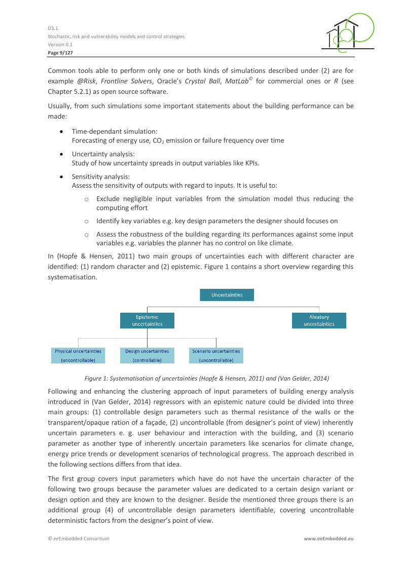
In (Hopfe & Hensen, 2011) two main groups of uncertainties each with different character are

identified: (1) random character and (2) epistemic. Figure 1 contains a short overview regarding this

systematisation.

Figure 1: Systematisation of uncertainties (Hopfe & Hensen, 2011) and (Van Gelder, 2014)

Following and enhancing the clustering approach of input parameters of building energy analysis

introduced in (Van Gelder, 2014) regressors with an epistemic nature could be divided into three

main groups: (1) controllable design parameters such as thermal resistance of the walls or the

transparent/opaque ration of a façade, (2) uncontrollable (from designer’s point of view) inherently

uncertain parameters e. g. user behaviour and interaction with the building, and (3) scenario

parameter as another type of inherently uncertain parameters like scenarios for climate change,

energy price trends or development scenarios of technological progress. The approach described in

the following sections differs from that idea.

The first group covers input parameters which have do not have the uncertain character of the

following two groups because the parameter values are dedicated to a certain design variant or

design option and they are known to the designer. Beside the mentioned three groups there is an

additional group (4) of uncontrollable design parameters identifiable, covering uncontrollable

deterministic factors from the designer’s point of view.

D3.1


Version 0.1

Page 10/127


(1) Controllable design parameters a. thermal resistance of the walls b. transparent/opaque ration of a façade c. layer structure, thickness and optical properties of a glazing system d. type and nominal capacity of a boiler, heat pump or CHP

(2) Uncontrollable inherently uncertain parameters a. User occupancy (Markov process) b. User behaviour c. Reliability / Malfunction (Poisson process)

(3) Uncontrollable inherently uncertain scenario parameters a. Technological progress (Wiener process) b. Climate trend (Wiener Process) c. Energy price (GARCH)

(4) Uncontrollable deterministic factors a. Site location b. International, national and regional design standards c. Public holidays

Depending on the main intensions addressed within Chapter 1.2 and the clustering introduced

above, certain parameters have to be modelled with the help of appropriate stochastic approaches

according to the type of analysis.

Within Chapter 1.3 certain models and approaches will be introduced in brief.

1.3 Overall structure and workflow of the design process of energy systems

The stepwise design approach which includes optimisation and embedded stochastic analysis covers

the following main subsystems of the building energy supply. These subsystems are core parts of the

energy systems information model (ESIM) shown in Figure 2 and described within (Kaiser et al.,

2015).

Figure 2: Core objects within the energy system information model ESIM

D3.1


Version 0.1

Page 11/127


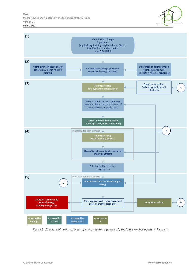
Figure 3 contains a schema which presents the overall workflow for designing, analysing as well as

optimising the energy generation and distribution system taking into account a broad variety of

influencing factors while elaborating a sophisticated and state-of-the-art as well as future-proof

energy system.

The approach is divided into several main working steps, each containing one or more subtasks. The

working steps are labelled with numbers (1) to (5) on the left margin of the coloured background

boxes. The boxes containing a brief description of the tasks and subtasks are coloured differently

regarding to the software tools which will be used to process the dedicated analysis. There is a

legend added on the bottom of the figure where the related software tools are named.

Within Figure 3 circles are placed containing the letters A, B, C, and D. These labels are anchor points

indicating links to Figure 4 which presents an overview of the considered regressors and their

assignment to stochastic processes. To ensure consistency between both figures, Figure 4 contains

the same labels (A) to (D). A brief explanation of the letters according to Figure 4 will be given below:

(A) Probable realisation of a Markov chain modelling the energy consumption of end energy for

heating/cooling and electricity

(B) Results of an estimation of end energy for heating / cooling and electricity and simulated

weather data as well as energy price

(C) Results of an estimation of the technological progress related to energy systems and building

envelop

(D) Results of an estimation of malfunction and a reliability scenario

D3.1


Version 0.1

Page 12/127


Figure 3: Structure of design process of energy systems (Labels (A) to (D) are anchor points to Figure 4)

D3.1


Version 0.1

Page 13/127


The starting point of the workflow which is marked with the label (1) in Figure 3 is the definition of

the following aspects:

1. Area which is characterized

a. Technology

i. Existing technology

ii. Future technology

b. Building

i. Building stock

ii. Preview on future re-vitalisation of the building sock

iii. Newly build rate

c. Energy infrastructure development

i. Streets

ii. Energy / media supply networks

iii. Introduction terms of new routes for heat and gas supply networks

2. Structure of prices and costs

d. Technology

i. Current investment and operational costs

ii. Volatilities

e. Energy prices

i. Curve of prices on the energy (stock) exchange during the last few years

ii. Already existing futures or forwards on energy

3. Local conditions

f. Weather / climate on the site location

g. Influences coming from the neighbourhood which infects the site location

4. Period under observation

h. E.g. 30 years

The second step within the workflow – marked with the label (2) in Figure 3 - covers the pre-

selection and localisation of the energy generators. Within this task a reasonable - and possibly

heterogeneous - portfolio containing a limited number of types of energy (heat and/or electricity)

generators is defined. To set-up a full scale matrix each of this energy generator types is described

with only a few variants of nominal power. Out of this matrix a certain number of combinations will

be selected to process a complete optimised application scenario based on a typical year of the

analysis period taking into account typical load curves for electricity and heat demand related to the

usage of the building. Within this step the optimisation is processed by the software tool FWOpt, see

Chapter 5.2.2. The typical load curves used within this working step will be defined without

variations. As a result of this step a set of energy generators which fits best to the supply tasks will be

identified and localized.

Within the third step of the workflow marked with the label (3) in Figure 3 the distribution networks

for heating energy and/or natural gas supply will be designed newly or enhanced with the help of the

software tool STEFaN, see Chapter 5.2.2. To develop a future-proof concept this design step takes

into consideration various numbers of scenarios of heating demand.

D3.1


Version 0.1

Page 14/127


Step four (4) in Figure 3 covers a second optimisation step considering various scenarios for energy

demand and energy prices in combination with various set-ups of energy generators. The certain

scenarios of energy demand will be elaborated with the software tool R-ARIMA. Scenarios for the

progression of the energy price will be processed by the software tool R-GARCH in case of short-term

prognosis (< 1 day) and R-ARIMA in case of a large time scale. As a result of this working step

approximated yearly costs for energy supply will be worked out for each of the analysed generator

set-ups and scenarios. Out of this range of values the less expensive set-up of energy generators will

be set as reference system. Chapter 5.2.1 contains a brief introduction to the software package R.

Within the fifth step (5) in Figure 3 different scenarios for the energy usage and the progression of

energy prices will be analysed with the help of the software tool TRNSYS-TUD (see Chapter 5.2.5) for

transient building and energy system simulation. Within the transient analysis scenarios for the

progression of technological progress related to the types of energy generation will be considered.

The analysis is taking into account the probabilistic character of the occupancy of people modelled by

the software tool R-birth-and-death within various types of buildings and the related indirect effects

like the selection of indoor temperature set-points and manual driven natural ventilation as well as

interaction with shading devices. Furthermore the individual operation of lighting and user specific

equipment within each analysis the individual operational schedule of each energy generator but

also the energy usage as well as the attached energy costs will be elaborated as time series.

The results are available for downstream analysis possibly covering the evaluation of the preferred

set-up with respect to common political or individual financial targets or analysis of operational

dependability processed by the software tool R-Poisson.

Figure 4 explains the localisation and interdependencies of the identified regressors. The regressors

will be introduced in more detail starting within Chapter 2.2.4.

D3.1


Version 0.1

Page 15/127


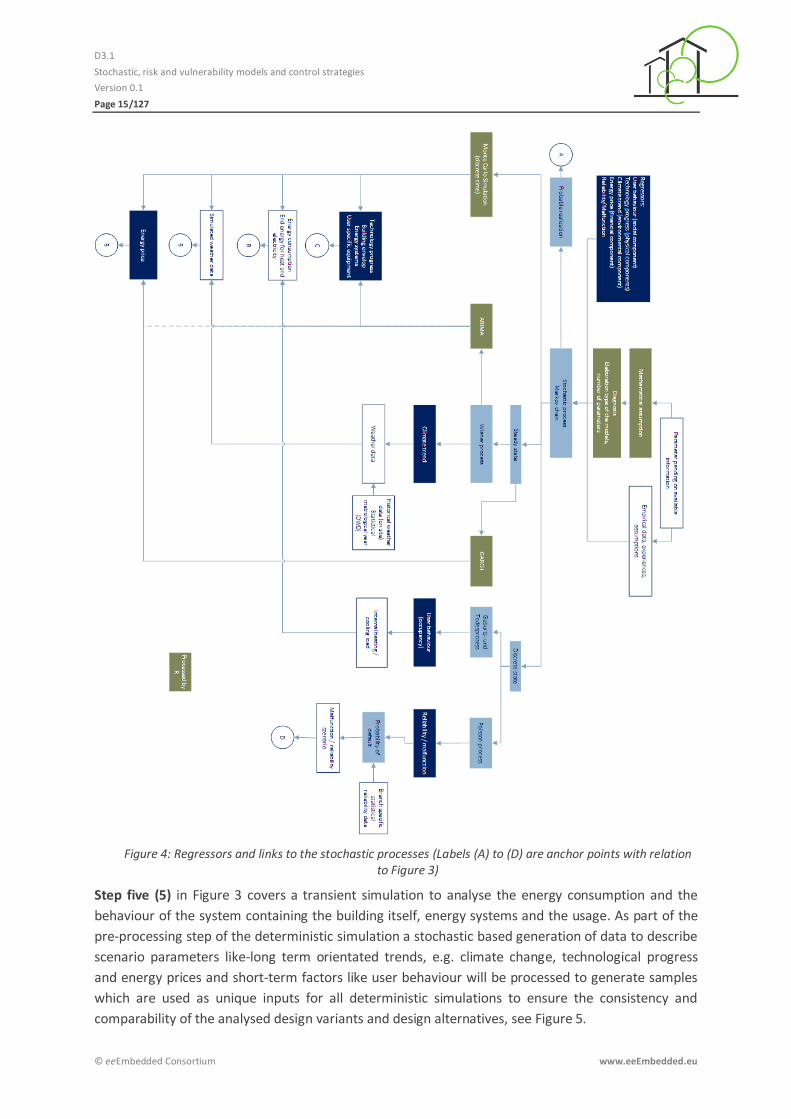
Figure 4: Regressors and links to the stochastic processes (Labels (A) to (D) are anchor points with relation to Figure 3)

Step five (5) in Figure 3 covers a transient simulation to analyse the energy consumption and the

behaviour of the system containing the building itself, energy systems and the usage. As part of the

pre-processing step of the deterministic simulation a stochastic based generation of data to describe

scenario parameters like-long term orientated trends, e.g. climate change, technological progress

and energy prices and short-term factors like user behaviour will be processed to generate samples

which are used as unique inputs for all deterministic simulations to ensure the consistency and

comparability of the analysed design variants and design alternatives, see Figure 5.

D3.1


Version 0.1

Page 16/127


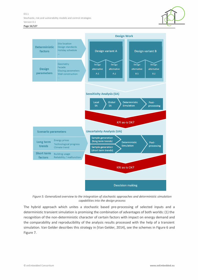
Figure 5: Generalized overview to the integration of stochastic approaches and deterministic simulation capabilities into the design process

The hybrid approach which unites a stochastic based pre-processing of selected inputs and a

deterministic transient simulation is promising the combination of advantages of both worlds: (1) the

recognition of the non-deterministic character of certain factors with impact on energy demand and

the comparability and reproducibility of the analysis results processed with the help of a transient

simulation. Van Gelder describes this strategy in (Van Gelder, 2014), see the schemes in Figure 6 and

Figure 7.

D3.1


Version 0.1

Page 17/127


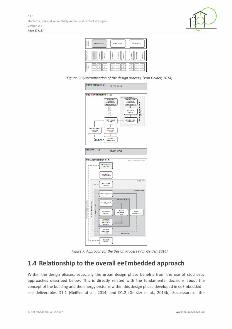
Figure 6: Systematisation of the design process, (Van Gelder, 2014)

Figure 7: Approach for the Design Process (Van Gelder, 2014)

1.4 Relationship to the overall eeEmbedded approach

Within the design phases, especially the urban design phase benefits from the use of stochastic

approaches described below. This is directly related with the fundamental decisions about the

concept of the building and the energy systems within this design phase developed in eeEmbedded -

see deliverables D1.1 (Geißler at al., 2014) and D1.2 (Geißler et al., 2014b). Successors of the

D3.1


Version 0.1

Page 18/127


stochastic analysis are the architect and the energy expert. Workflow related points are mentioned

above. The stochastic analysis fits seamlessly into the design workflow.

Based on the conceptual nature of the urban design phase a high number of certain kinds of

templates will be used to speed-up the design process. This concept is adaptable to the stochastic

analysis as mentioned in eeEmbedded Deliverable D1.4 (Solvik et al., 2014). In conjunction with the

template concept and the ESIM concept which will contain information about

reliability/dependability the stochastic analysis can be easily included in the overall framework. The

strong cloud-orientated approach of eeEmbedded described in deliverable D1.5 (Zellner et al., 2014)

provides the needed analysis capabilities and computing power to use the stochastic analysis

approaches in a worthwhile manner.

There are certain links from T3.1 to T3.3, respectively D3.1 to eeEmbedded deliverable D3.2, as well

as eeEmbedded work packages WP5 and WP6.

D3.1


Version 0.1

Page 19/127


2 Stochastic models and approaches

2.1 Introducing stochastic processes

Stochastic processes are defined as processes which are not exclusively deterministic, taking into

account one or more probabilistic variables. A stochastic process is represented as a set of

probabilistic values depending on parameter with passing through a parameter space. The

parameter could represent the time or have any other meaning. Beside there could be other

additional parameters too (Meyna & Pauli, 2010).

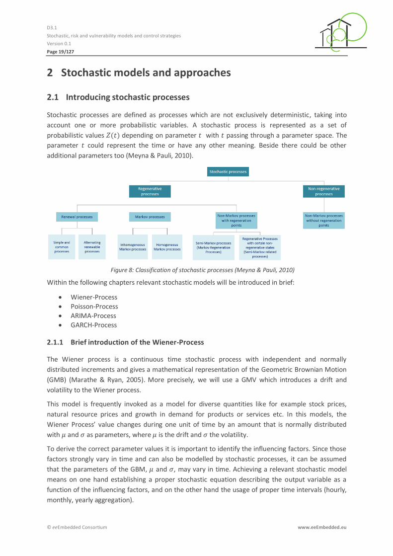
Figure 8: Classification of stochastic processes (Meyna & Pauli, 2010)

Within the following chapters relevant stochastic models will be introduced in brief:

Wiener-Process

Poisson-Process

ARIMA-Process

GARCH-Process

Brief introduction of the Wiener-Process 2.1.1

The Wiener process is a continuous time stochastic process with independent and normally

distributed increments and gives a mathematical representation of the Geometric Brownian Motion

(GMB) (Marathe & Ryan, 2005). More precisely, we will use a GMV which introduces a drift and

volatility to the Wiener process.

This model is frequently invoked as a model for diverse quantities like for example stock prices,

natural resource prices and growth in demand for products or services etc. In this models, the

Wiener Process’ value changes during one unit of time by an amount that is normally distributed

with and as parameters, where is the drift and the volatility.

To derive the correct parameter values it is important to identify the influencing factors. Since those

factors strongly vary in time and can also be modelled by stochastic processes, it can be assumed

that the parameters of the GBM, and , may vary in time. Achieving a relevant stochastic model

means on one hand establishing a proper stochastic equation describing the output variable as a

function of the influencing factors, and on the other hand the usage of proper time intervals (hourly,

monthly, yearly aggregation).

D3.1


Version 0.1

Page 20/127


One example of an approach using the Wiener-Process for forecasting building energy consumption

is drawn in (Brohus et. al., 2012). The authors set up a system of stochastic differential equations

(SDE) describing incremental load changes, by which variables like external and internal

temperatures, convective and radiation heat flows and heat losses, are defined by a Wiener

processes like follows:

where , the “white noise” characterising the Wiener-Process.

The common way of identifying parameters of stochastic processes would be to use historical data. It

can be assumed that a lack of such data exists in most cases.

Brief introduction of the Poisson-Process 2.1.2

The Poisson-Process is a type of birth-death-process covering only birth events. Within this process

the occurrence of certain events according to the point of time of their occurrence within a time

interval is modelled. The Poisson process depends on only one parameter, , which gives the rate of

occurences for every point in time (e.g. a hazard rate). The events and the time of their occurrence

are independent from each other. The time between the events follows an exponential distribution

with the parameter .

Poisson processes are used to model the occurrence of malfunction within dependability analysis and

as approximation for the binomial distribution (Bernoulli distribution).

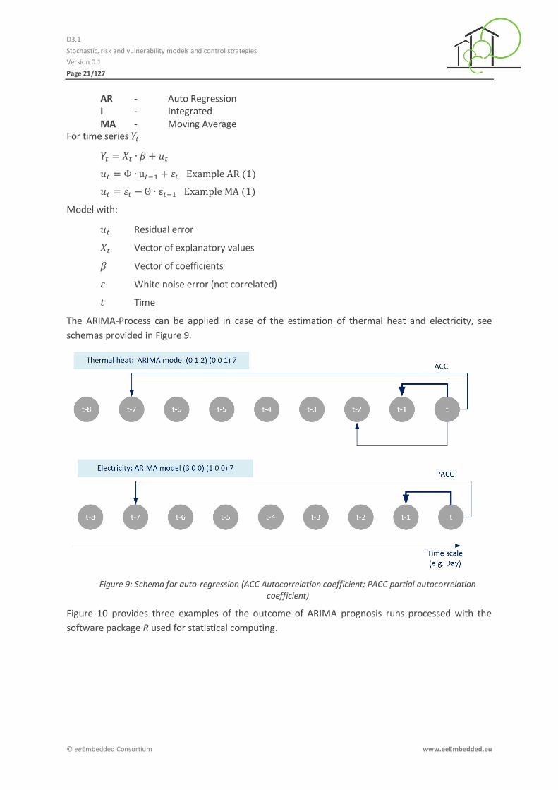
Brief description of the ARIMA-Process 2.1.3

ARMA is the abbreviation of AutoRegressive-Moving Average. The notation stands for

Auto-regressive terms

Moving-average terms

The common formulation of the equation has the following form:

∑

∑

ARMA is a subset of the process with . It stands for linear models for steady

state, time discrete stochastic processes. These processes are used for time series analysis within

prognosis models regarding financial and economic issues.

This approach covers the analysis of a single time series or a set of time series describing the

behaviour of certain indicators of interest. The ARIMA-Process is focused on the differences between

the values of the prognosis and needs an integration step after the prognosis is done.

In the mathematical sense the ARIMA models are linear difference equations or systems of

equations.

The ARIMA-Process is characterized by the parameters , and and is considered when the ARMA-

Process is applied to the times differentiated time series . The notation is .

ARIMA Model

D3.1


Version 0.1

Page 21/127


AR - Auto Regression I - Integrated MA - Moving Average

For time series

Model with:

Residual error

Vector of explanatory values

Vector of coefficients

White noise error (not correlated)

Time

The ARIMA-Process can be applied in case of the estimation of thermal heat and electricity, see

schemas provided in Figure 9.

Figure 9: Schema for auto-regression (ACC Autocorrelation coefficient; PACC partial autocorrelation coefficient)

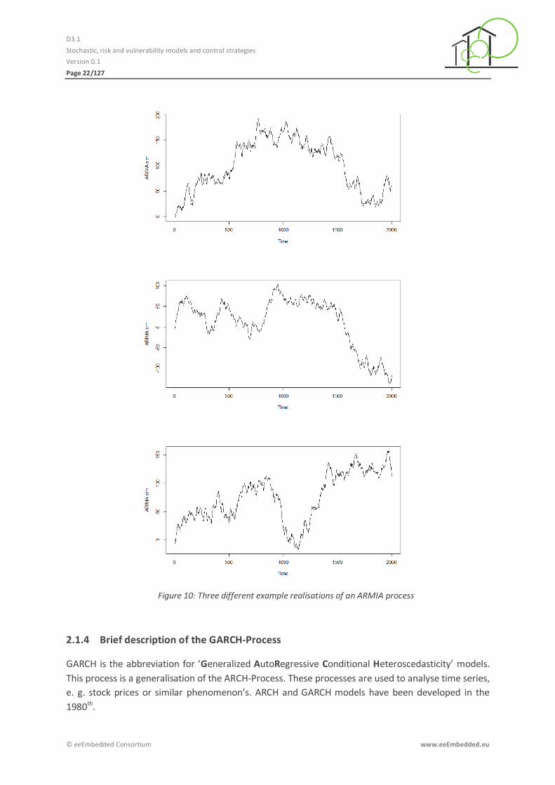
Figure 10 provides three examples of the outcome of ARIMA prognosis runs processed with the

software package R used for statistical computing.

D3.1


Version 0.1

Page 22/127


Figure 10: Three different example realisations of an ARMIA process

Brief description of the GARCH-Process 2.1.4

GARCH is the abbreviation for ‘Generalized AutoRegressive Conditional Heteroscedasticity’ models.

This process is a generalisation of the ARCH-Process. These processes are used to analyse time series,

e. g. stock prices or similar phenomenon’s. ARCH and GARCH models have been developed in the

1980th.

D3.1


Version 0.1

Page 23/127


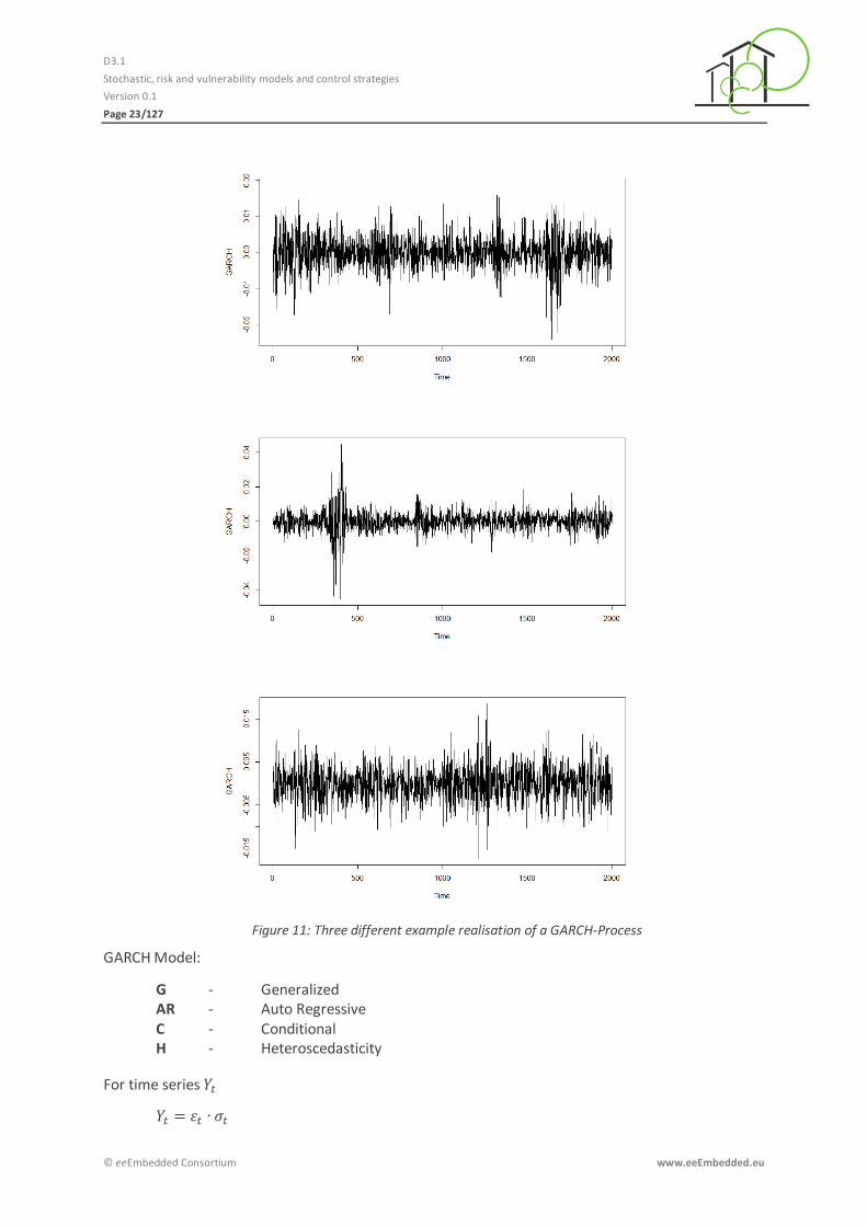
Figure 11: Three different example realisation of a GARCH-Process

GARCH Model:

G - Generalized AR - Auto Regressive C - Conditional H - Heteroscedasticity

For time series

D3.1


Version 0.1

Page 24/127


The model is given by the following terms

or in a aggregated manner

∑

∑

or in other form

Modell with:

Order of GARCH terms

Order of ARCH terms

Vector of Regression coefficients

Vector of Regression coefficients

White noise error (not correlated)

Time

2.2 Forecasting energy consumption

Clustering of factors with high impact on energy consumption 2.2.1

In general the energy consumption for heating/cooling and electricity of a building is influenced by

several internal and external factors. These factors could be categorized into several main clusters.

Figure 12 categorizes the main factors with the most impact on energy related prognosis in a general

manner: (1) physical factors with strong relation to weather and climate phenomenon’s, but also (2)

historical factors especially if existing energy systems or buildings have to be integrated and/or

enhanced, (3) social factors covering the usage scenarios in general and other factors with an

random nature.

Figure 12: Groups of parameters within a prognosis

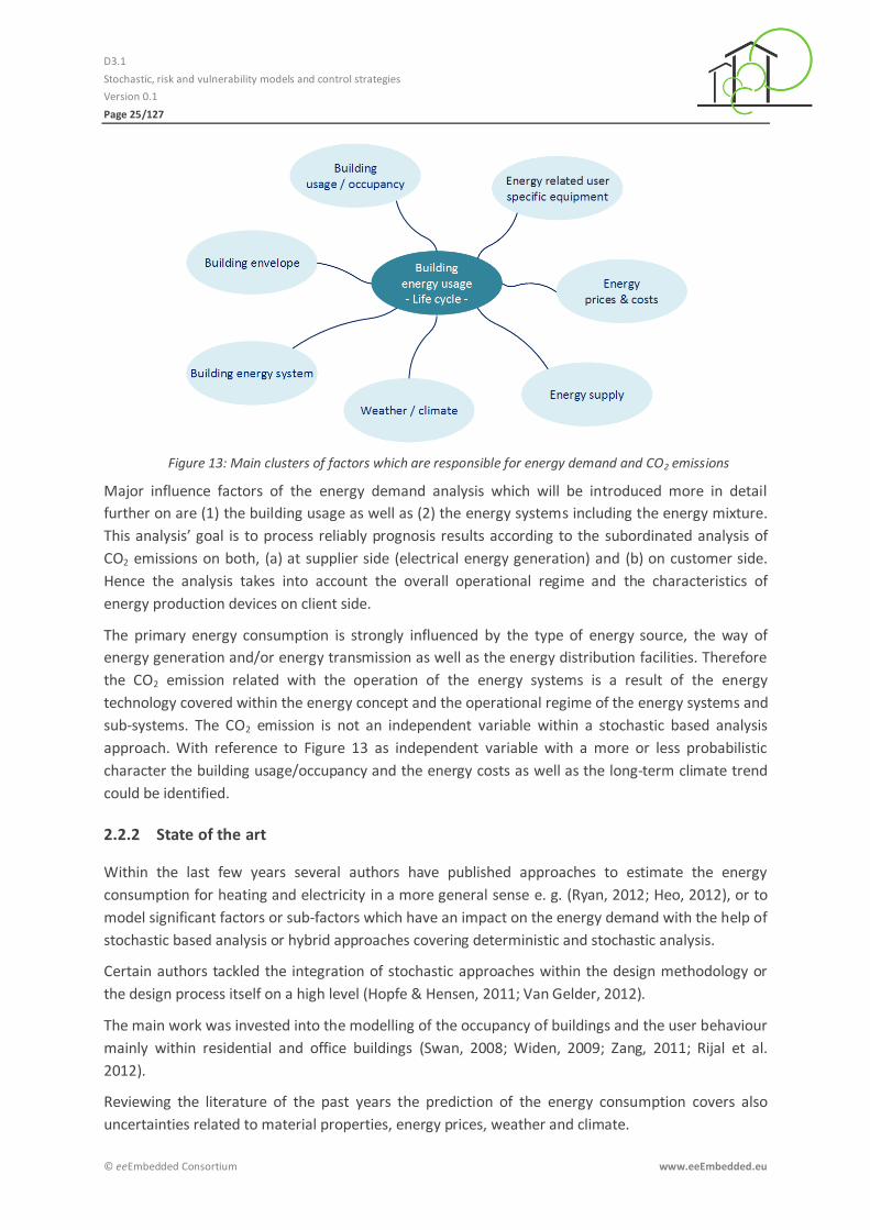
Figure 13 gives a high-level overview about these clusters without the intention to be exhaustive. To

reduce complexity not all existing interdependencies between these clusters are addressed within

this figure.

D3.1


Version 0.1

Page 25/127


Figure 13: Main clusters of factors which are responsible for energy demand and CO2 emissions

Major influence factors of the energy demand analysis which will be introduced more in detail

further on are (1) the building usage as well as (2) the energy systems including the energy mixture.

This analysis’ goal is to process reliably prognosis results according to the subordinated analysis of

CO2 emissions on both, (a) at supplier side (electrical energy generation) and (b) on customer side.

Hence the analysis takes into account the overall operational regime and the characteristics of

energy production devices on client side.

The primary energy consumption is strongly influenced by the type of energy source, the way of

energy generation and/or energy transmission as well as the energy distribution facilities. Therefore

the CO2 emission related with the operation of the energy systems is a result of the energy

technology covered within the energy concept and the operational regime of the energy systems and

sub-systems. The CO2 emission is not an independent variable within a stochastic based analysis

approach. With reference to Figure 13 as independent variable with a more or less probabilistic

character the building usage/occupancy and the energy costs as well as the long-term climate trend

could be identified.

State of the art 2.2.2

Within the last few years several authors have published approaches to estimate the energy

consumption for heating and electricity in a more general sense e. g. (Ryan, 2012; Heo, 2012), or to

model significant factors or sub-factors which have an impact on the energy demand with the help of

stochastic based analysis or hybrid approaches covering deterministic and stochastic analysis.

Certain authors tackled the integration of stochastic approaches within the design methodology or

the design process itself on a high level (Hopfe & Hensen, 2011; Van Gelder, 2012).

The main work was invested into the modelling of the occupancy of buildings and the user behaviour

mainly within residential and office buildings (Swan, 2008; Widen, 2009; Zang, 2011; Rijal et al.

2012).

Reviewing the literature of the past years the prediction of the energy consumption covers also

uncertainties related to material properties, energy prices, weather and climate.

D3.1


Version 0.1

Page 26/127


There are several tools available for processing analysis and prognosis of energy consumption based

on simplified benchmark-based approaches, e. g. RETscreen, CASAnova, IWU Kurzverfahren Energie-

profil.

Prognosis of energy demand as part of the design workflow 2.2.3

At first before starting a prognosis of energy demand clarification is needed about the duration of

the assumed analysis period and depending on that the consideration of refurbishment activities

over the lifecycle period under focus. With reference to the building lifecycle an implied period of 30

years for the analysis seems to be a reasonable value.

There are tools available for short- (hours to a few days) and medium-term (one to several years)

prognosis which have to be enhanced for taking into account long-term trends covering more than a

few years according to the building lifecycle.

Existing and newly developed tools are assembled to build up a toolbox to support all design steps

which are arranged within the schema given in Figure 3. The overall target is the development of an

automated processable workflow to support and finally speed-up the overall design workflow as well

as minimising manual interferences.

The overall progression of the energy demand will be analysed with the help of deterministic

simulations in combination with pre-processed variables using stochastic processes without memory

– so called Markov processes. A known representative and special case of this process is the Wiener-

Process which is concurrently a marginal case of the ARIMA model too.

The particular involved simulation will be performed based on a discretisation of time to simulate so

called Markov chains. Based on the main target the simulation will be performed using different time

steps, e. g. one day for short-term prognosis of the final energy - like in eeEmbedded project - or one

year or five-year time steps which is not in focus within eeEmbedded.

Within the early design stages there is only a rough picture available as input for the elaboration of

an energy concept about (1) the building geometry, (2) the construction details and (3) the future

usage of the building. For this case standardised load profiles for electrical energy and natural gas

supply are available to bridge this gap. These profiles are described within (BDEW, 20079 and (E-

Control, 2011). In the case that more accurate and validated data is available, this values should be

used instead of the standardised load profiles. The standard load profiles will be used for generating

individual load profiles taking into account the influence of outside air temperature throughout the

day, the type of day (business day, Saturday, Sunday / public holiday), but also the type of usage

(several kinds of pre-defined business branches, household and others) based on a Sigmoid function,

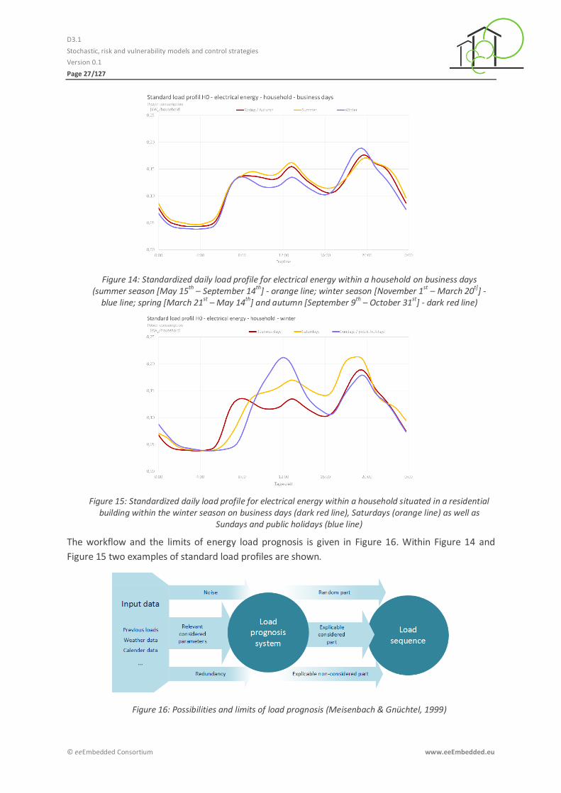
see Figure 14 and Figure 15.

D3.1


Version 0.1

Page 27/127


Figure 14: Standardized daily load profile for electrical energy within a household on business days (summer season [May 15

th – September 14

th] - orange line; winter season [November 1

st – March 20

t]] -

blue line; spring [March 21st – May 14th] and autumn [September 9th – October 31st] - dark red line)

Figure 15: Standardized daily load profile for electrical energy within a household situated in a residential building within the winter season on business days (dark red line), Saturdays (orange line) as well as

Sundays and public holidays (blue line)

The workflow and the limits of energy load prognosis is given in Figure 16. Within Figure 14 and

Figure 15 two examples of standard load profiles are shown.

Figure 16: Possibilities and limits of load prognosis (Meisenbach & Gnüchtel, 1999)

D3.1


Version 0.1

Page 28/127


There are several common working steps identified within the workflow:

(1) Preliminary investigation including sample survey with the following subtasks

a. Concept development for the prognosis model

b. Data capture and data verification

(2) Identification of the prognosis model

a. Elaboration of dependencies

b. Selection of the prognosis model

c. Selection of the input values

(3) Adaptation of the model

a. Ascertainment of free parameters

(4) Back-interpretation and check

(5) Processing of the prognosis

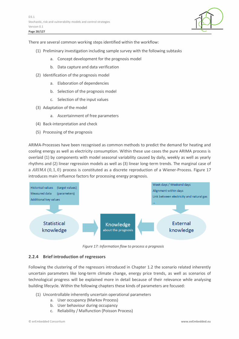
ARIMA-Processes have been recognised as common methods to predict the demand for heating and

cooling energy as well as electricity consumption. Within these use cases the pure ARIMA process is

overlaid (1) by components with model seasonal variability caused by daily, weekly as well as yearly

rhythms and (2) linear regression models as well as (3) linear long-term trends. The marginal case of

a process is constituted as a discrete reproduction of a Wiener-Process. Figure 17

introduces main influence factors for processing energy prognosis.

Figure 17: Information flow to process a prognosis

Brief introduction of regressors 2.2.4

Following the clustering of the regressors introduced in Chapter 1.2 the scenario related inherently

uncertain parameters like long-term climate change, energy price trends, as well as scenarios of

technological progress will be explained more in detail because of their relevance while analysing

building lifecycle. Within the following chapters these kinds of parameters are focused:

(1) Uncontrollable inherently uncertain operational parameters a. User occupancy (Markov Process) b. User behaviour during occupancy c. Reliability / Malfunction (Poisson Process)

D3.1


Version 0.1

Page 29/127


(2) Uncontrollable inherently uncertain scenario parameters a. Technological progress (Wiener process) b. Climate trend (Wiener Process) c. Energy price (GARCH)

In Table 1 to

D3.1


Version 0.1

Page 30/127


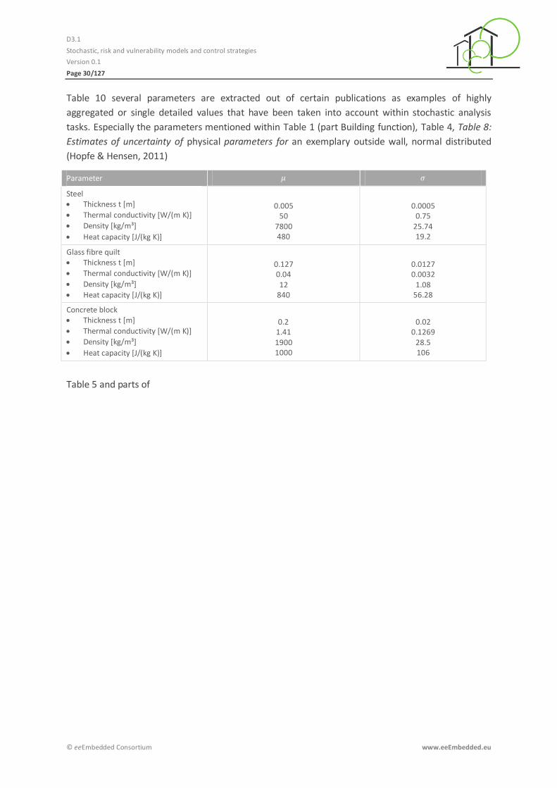
Table 10 several parameters are extracted out of certain publications as examples of highly

aggregated or single detailed values that have been taken into account within stochastic analysis

tasks. Especially the parameters mentioned within Table 1 (part Building function), Table 4, Table 8:

Estimates of uncertainty of physical parameters for an exemplary outside wall, normal distributed

(Hopfe & Hensen, 2011)

Parameter

Steel Thickness t [m]

Thermal conductivity [W/(m K)]

Density [kg/m³]

Heat capacity [J/(kg K)]

0.005 50

7800 480

0.0005 0.75

25.74 19.2

Glass fibre quilt Thickness t [m]


Density [kg/m³]


0.127 0.04 12

840

0.0127 0.0032

1.08 56.28

Concrete block Thickness t [m]


Density [kg/m³]


0.2 1.41 1900 1000

0.02 0.1269

28.5 106

Table 5 and parts of

D3.1


Version 0.1

Page 31/127


Table 7 (internal loads, ventilation), as well as values given in Table 6 are applicable within the

stochastic related approach described in this document.

Table 1: Sensitivity parameters, extract of (Hoes, 2008)

Parameter Min Mean Max SD

Building function and type of user

Occupant per floor area [m²/occupant]

Occupant mobility [R]

4.3

1

11.1

4

22.8

8

3.1

1.2

Building concept (passive / active system)

Building response time; Specific active mass (kg/m²]

Active system response time Maximum heating load [W] Maximum cooling load [W]

Window size in façade Percentage of transparency total façade [%]

Influence of outdoor environment in indoor environment; Heat transfer through transparent construction

Solar heat gain - g-value [-]

Size transparent surfaces [m²]

Heat transfer coefficient - U-value [W/(m² K]

Heat transport through opaque construction thermal resistance (R-value) [(m²K)/W]

Daylight gains light transmittance [-]

Heat gains lighting [W/m²]

Heat gains apparatus [W/m²]

5

200 300

6

0.40 -

1.2

1.3

0.7 6.2 5.7

50

500 650

35

0.60 -

2.1

2.5

0.75 12.7 17.5

100

800

1250

100

0.85 -

3.0

4.0

0.80 33.9 34.0

15.8

100 150

15.7

0.10 -

0.3

0.5

0.0 4.6 4.7

Table 2: Design scenario parameters (Hopfe & Hensen, 2011)

Parameter

Room size [m²] [182,325]

Switch between single / double glazing yes/no

Table 3: Design scenario parameters, extract of (Van Gelder, 2014)

Parameter Discrete scenario values Reference

Nominal energy price evolution -1.5 % / +2.3 % / +10 % Van Gelder, 2014

Table 4: Stochastic design parameters, extract of (Van Gelder, 2014)

Parameter Distribution Reference

Air infiltration rate at 50 Pa l/h Van Gelder, 2014

Heat recovery rate of the ventilation system

Van Gelder, 2014

D3.1


Version 0.1

Page 32/127


Legend

Uniform distribution between a and b

Normal distribution with mean value and standard deviation

Weibull deviation with scale factor and shape factor

Additional comment Discrete uniform distributions are indicated by the same values

Table 5: Uncertainty parameters, extract of (Van Gelder, 2014)

Parameter Distribution Reference

Set temperature occupancy day zone °C Van Gelder, 2014

Set temperature absence day zone 15°C, no reduction Van Gelder, 2014

Set temperature occupancy night zone °C Van Gelder, 2014

Internal heat gains W Van Gelder, 2014

Air change rate day zone 1/h Van Gelder, 2014

Air change rate night zone 1/h Van Gelder, 2014

Legend

Uniform distribution between a and b

Normal distribution with mean value and standard deviation

Weibull deviation with scale factor and shape factor

Additional comment Discrete uniform distributions are indicated by the same values

Table 6: Estimation of uncertainty of parameters related to thermal load or operation regime, normal distributed (Hopfe & Hensen, 2011)

Parameter

Infiltration AC Rate [ACH] 0.5 0.17

Loads people [W/m²] 15 2.4

Loads lighting [W/m²] 15 2.4

Loads equipment [W/m²] 20 3.2

Glass surface [%] 75 22.5

D3.1


Version 0.1

Page 33/127


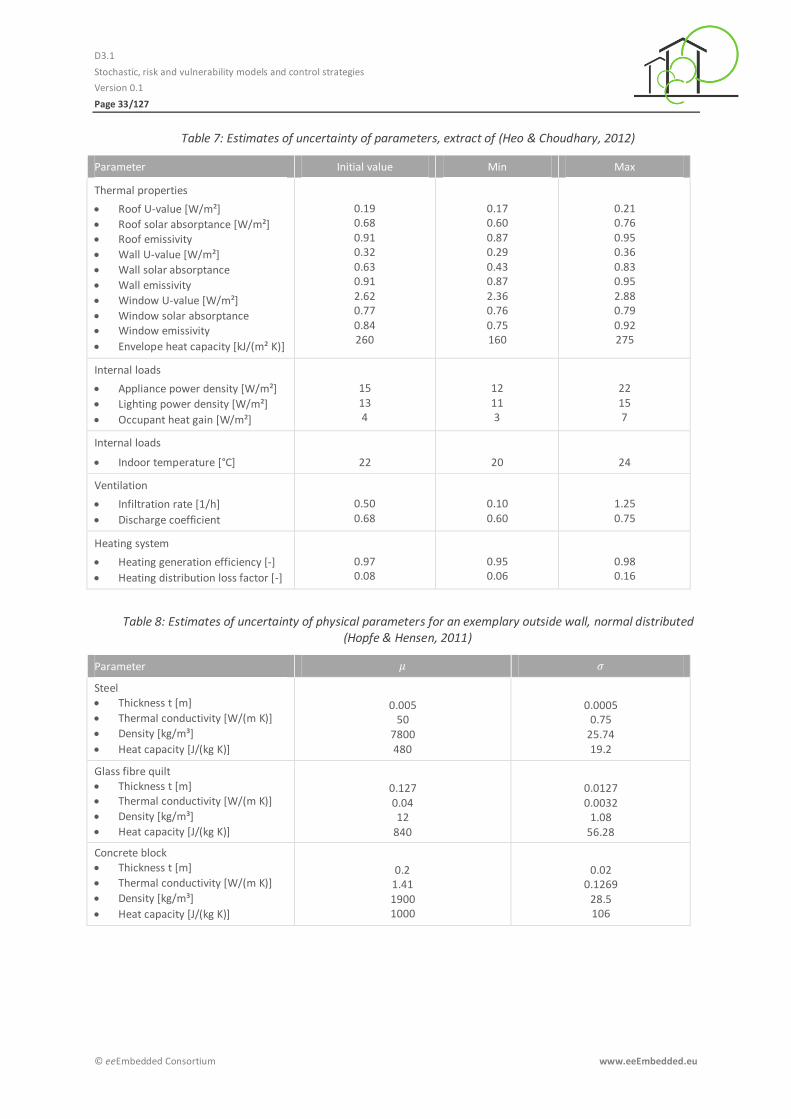
Table 7: Estimates of uncertainty of parameters, extract of (Heo & Choudhary, 2012)

Parameter Initial value Min Max

Thermal properties

Roof U-value [W/m²]

Roof solar absorptance [W/m²] Roof emissivity

Wall U-value [W/m²]

Wall solar absorptance

Wall emissivity

Window U-value [W/m²]

Window solar absorptance Window emissivity

Envelope heat capacity [kJ/(m² K)]

0.19 0.68 0.91 0.32 0.63 0.91 2.62 0.77 0.84 260

0.17 0.60 0.87 0.29 0.43 0.87 2.36 0.76 0.75 160

0.21 0.76 0.95 0.36 0.83 0.95 2.88 0.79 0.92 275

Internal loads

Appliance power density [W/m²]

Lighting power density [W/m²]

Occupant heat gain [W/m²]

15 13 4

12 11 3

22 15 7

Internal loads

Indoor temperature [°C] 22 20 24

Ventilation

Infiltration rate [1/h]

Discharge coefficient

0.50 0.68

0.10 0.60

1.25 0.75

Heating system

Heating generation efficiency [-]

Heating distribution loss factor [-]

0.97 0.08

0.95 0.06

0.98 0.16

Table 8: Estimates of uncertainty of physical parameters for an exemplary outside wall, normal distributed (Hopfe & Hensen, 2011)

Parameter

Steel Thickness t [m]


Density [kg/m³]


0.005 50

7800 480

0.0005 0.75

25.74 19.2

Glass fibre quilt Thickness t [m] Thermal conductivity [W/(m K)]

Density [kg/m³]


0.127 0.04 12

840

0.0127 0.0032

1.08 56.28

Concrete block Thickness t [m]


Density [kg/m³]


0.2 1.41 1900 1000

0.02 0.1269

28.5 106

D3.1


Version 0.1

Page 34/127


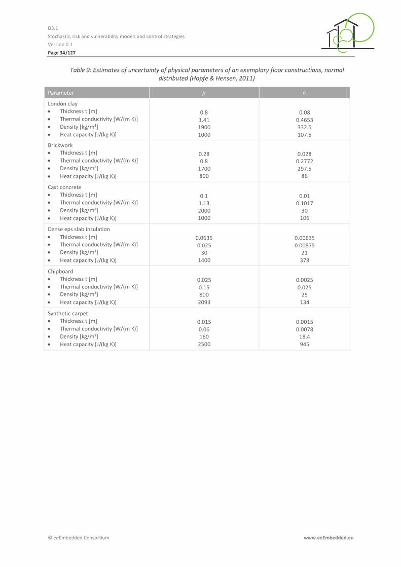
Table 9: Estimates of uncertainty of physical parameters of an exemplary floor constructions, normal distributed (Hopfe & Hensen, 2011)

Parameter

London clay Thickness t [m]


Density [kg/m³]


0.8 1.41 1900 1000

0.08 0.4653 332.5 107.5

Brickwork Thickness t [m]


Density [kg/m³]


0.28 0.8

1700 800

0.028 0.2772 297.5

86

Cast concrete Thickness t [m]


Density [kg/m³]


0.1 1.13 2000 1000

0.01 0.1017

30 106

Dense eps slab insulation

Thickness t [m] Thermal conductivity [W/(m K)]

Density [kg/m³]


0.0635 0.025

30 1400

0.00635 0.00875

21 378

Chipboard Thickness t [m]

Thermal conductivity [W/(m K)] Density [kg/m³]


0.025 0.15 800

2093

0.0025 0.025

25 134

Synthetic carpet Thickness t [m]


Density [kg/m³]


0.015 0.06 160

2500

0.0015 0.0078

18.4 945

D3.1


Version 0.1

Page 35/127


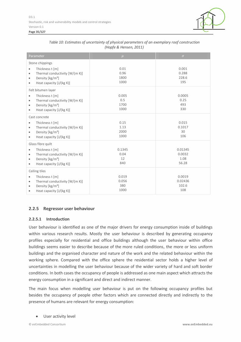
Table 10: Estimates of uncertainty of physical parameters of an exemplary roof construction (Hopfe & Hensen, 2011)

Parameter

Stone chippings

Thickness t [m] Thermal conductivity [W/(m K)]

Density [kg/m³]


0.01 0.96 1800 1000

0.001 0.288 228.6 195

Felt bitumen layer

Thickness t [m]


Density [kg/m³]


0.005 0.5

1700 1000

0.0005 0.25 493 330

Cast concrete

Thickness t [m]


Density [kg/m³]


0.15 1.13 2000 1000

0.015 0.1017

30 106

Glass fibre quilt

Thickness t [m]


Density [kg/m³]


0.1345 0.04 12

840

0.01345 0.0032

1.08 56.28

Ceiling tiles

Thickness t [m]

Thermal conductivity [W/(m K)] Density [kg/m³]


0.019 0.056 380

1000

0.0019 0.02436

102.6 108

Regressor user behaviour 2.2.5

2.2.5.1 Introduction

User behaviour is identified as one of the major drivers for energy consumption inside of buildings

within various research results. Mostly the user behaviour is described by generating occupancy

profiles especially for residential and office buildings although the user behaviour within office

buildings seems easier to describe because of the more ruled conditions, the more or less uniform

buildings and the organised character and nature of the work and the related behaviour within the

working sphere. Compared with the office sphere the residential sector holds a higher level of

uncertainties in modelling the user behaviour because of the wider variety of hard and soft border

conditions. In both cases the occupancy of people is addressed as one main aspect which attracts the

energy consumption in a significant and direct and indirect manner.

The main focus when modelling user behaviour is put on the following occupancy profiles but

besides the occupancy of people other factors which are connected directly and indirectly to the

presence of humans are relevant for energy consumption:

User activity level

D3.1


Version 0.1

Page 36/127


Occupancy

o Density

o Occurrence

User interaction with

o User equipment

Usage of user specific equipment

o Building components

Shading

Natural ventilation / Window opening

o HVAC / electrical systems

Lighting

Temperature set point

Ventilation set point

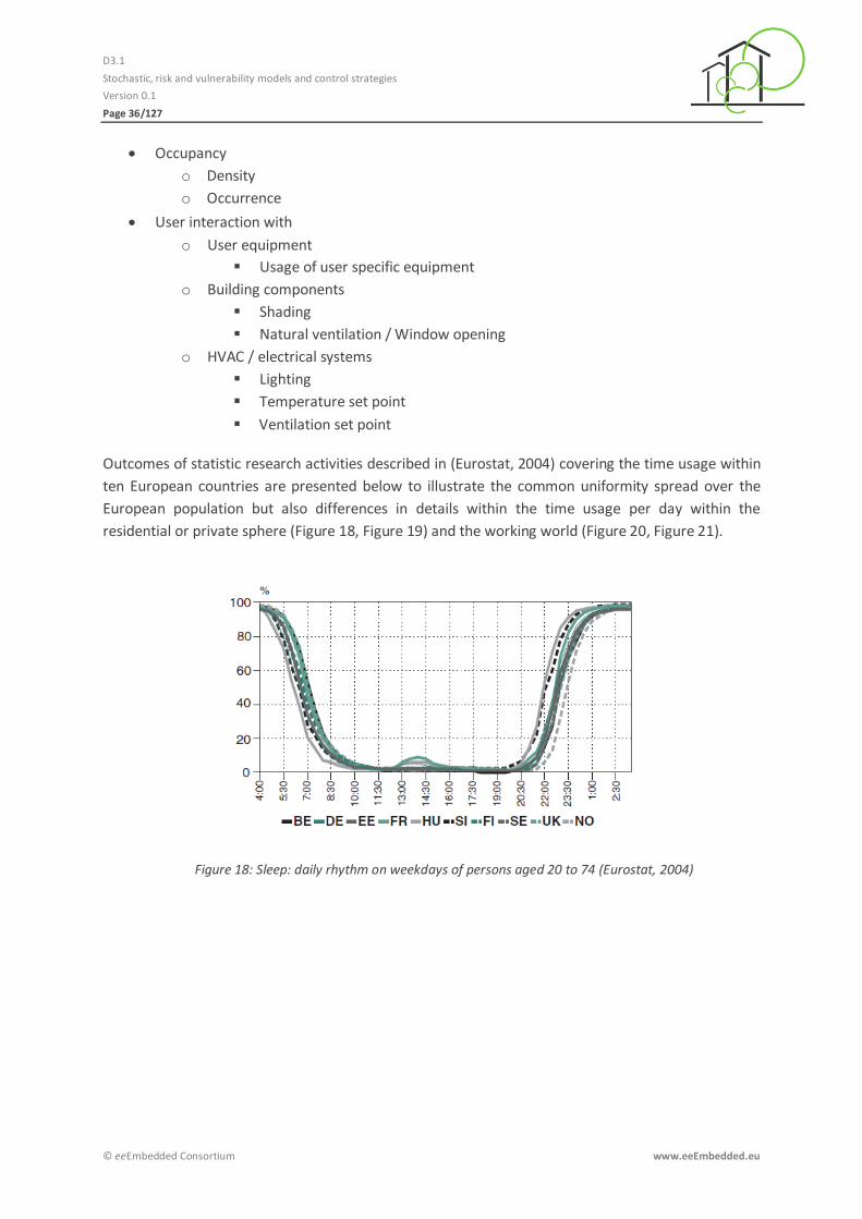
Outcomes of statistic research activities described in (Eurostat, 2004) covering the time usage within

ten European countries are presented below to illustrate the common uniformity spread over the

European population but also differences in details within the time usage per day within the

residential or private sphere (Figure 18, Figure 19) and the working world (Figure 20, Figure 21).

Figure 18: Sleep: daily rhythm on weekdays of persons aged 20 to 74 (Eurostat, 2004)

D3.1


Version 0.1

Page 37/127


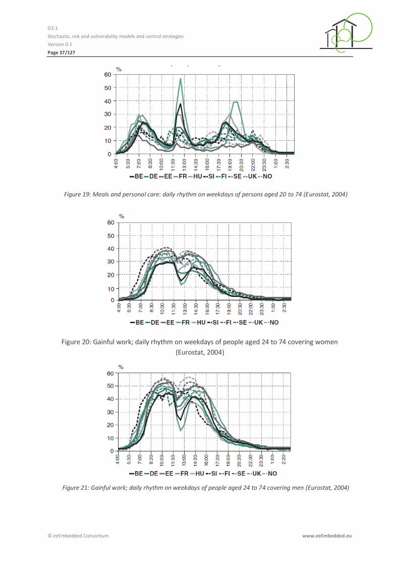
Figure 19: Meals and personal care: daily rhythm on weekdays of persons aged 20 to 74 (Eurostat, 2004)

Figure 20: Gainful work; daily rhythm on weekdays of people aged 24 to 74 covering women

(Eurostat, 2004)

Figure 21: Gainful work; daily rhythm on weekdays of people aged 24 to 74 covering men (Eurostat, 2004)

D3.1


Version 0.1

Page 38/127


2.2.5.2 Occupancy modelling

Within the past few years a great amount of research and analysis work was done to observe and

model the user behaviour within different types of buildings or to take into account the user’s

occupancy in relation to the energy demand within buildings, e.g. (Richardson et al., 2008; Page,

2008; Ipsos-RSL, 2000; Duarte et al., 2013; Yun et al., 2009; Rijal et al., 2007; van Den Wymelenberg,

2012; Guerra Santin, 2011; Hoes, 2009; Martani, 2012; Zhang et al., 2011; Bourgeois et al., 2006;

Widén et al., 2009; Virote, 2012; Humphreys & Nicol, 2002).

To model user behaviour, two steps are needed. At first, an occupancy model simulates the number

of people in every zone at every given time. Secondly, interaction models represent the possible

interactions of occupants with their environment, e.g. with the BACS or the lighting.

In the mathematical modelling of occupancy, two distinct approaches are dominant. One is agent-

based modelling, which simulates every single occupant individually see e.g. (Liao et al., 2010). The

major upside of this approach is the possibility of an extremely high level of detail. Furthermore the

dependence between zones, meaning that a person who is in one room cannot be in another, is

captured. The major downside is very high computational costs.

As occupancy simulation is only one of many tools in eeEmbedded, we decided for the

computationally efficient method of inhomogeneous first-order Markov chain models, which

simulates the number of occupants per zone forthrightly see e.g. (Richardson et al., 2008).

The term first-order Markov chain implies that the number of occupants in a zone at an arbitrary

time only depends on the state at time and the probability of transition between the states.

In mathematical terms, this is

| | .

The term inhomogeneous implies that these probabilities of transition depend on the current point

of time.

In the earlier design stages (urban design phase), it is possible that a zone is a floor or even the whole

building, while in later design stages (early and detailed design phase) with more information

available, a zone will be a special type of room like a manager’s office.

Additionally each zone has an associated level of activity, which is assigned to every occupant in the

zone. A zone with very high activity is e.g. a gym, while a bedroom is an example for a zone with a

low level of activity. These activity levels are used to estimate a person’s heat emission during the

energy simulation.

To simulate the number of occupants in a zone over the course of a day, all that is needed is a matrix

for every time step, containing the probabilities to transition between all possible states. Such a set

of matrices, belonging to one single zone, is called a zone profile.

D3.1


Version 0.1

Page 39/127


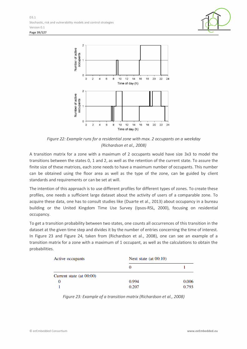
Figure 22: Example runs for a residential zone with max. 2 occupants on a weekday

(Richardson et al., 2008)

A transition matrix for a zone with a maximum of 2 occupants would have size 3x3 to model the

transitions between the states 0, 1 and 2, as well as the retention of the current state. To assure the

finite size of these matrices, each zone needs to have a maximum number of occupants. This number

can be obtained using the floor area as well as the type of the zone, can be guided by client

standards and requirements or can be set at will.

The intention of this approach is to use different profiles for different types of zones. To create these

profiles, one needs a sufficient large dataset about the activity of users of a comparable zone. To

acquire these data, one has to consult studies like (Duarte et al., 2013) about occupancy in a bureau

building or the United Kingdom Time Use Survey (Ipsos-RSL, 2000), focusing on residential

occupancy.

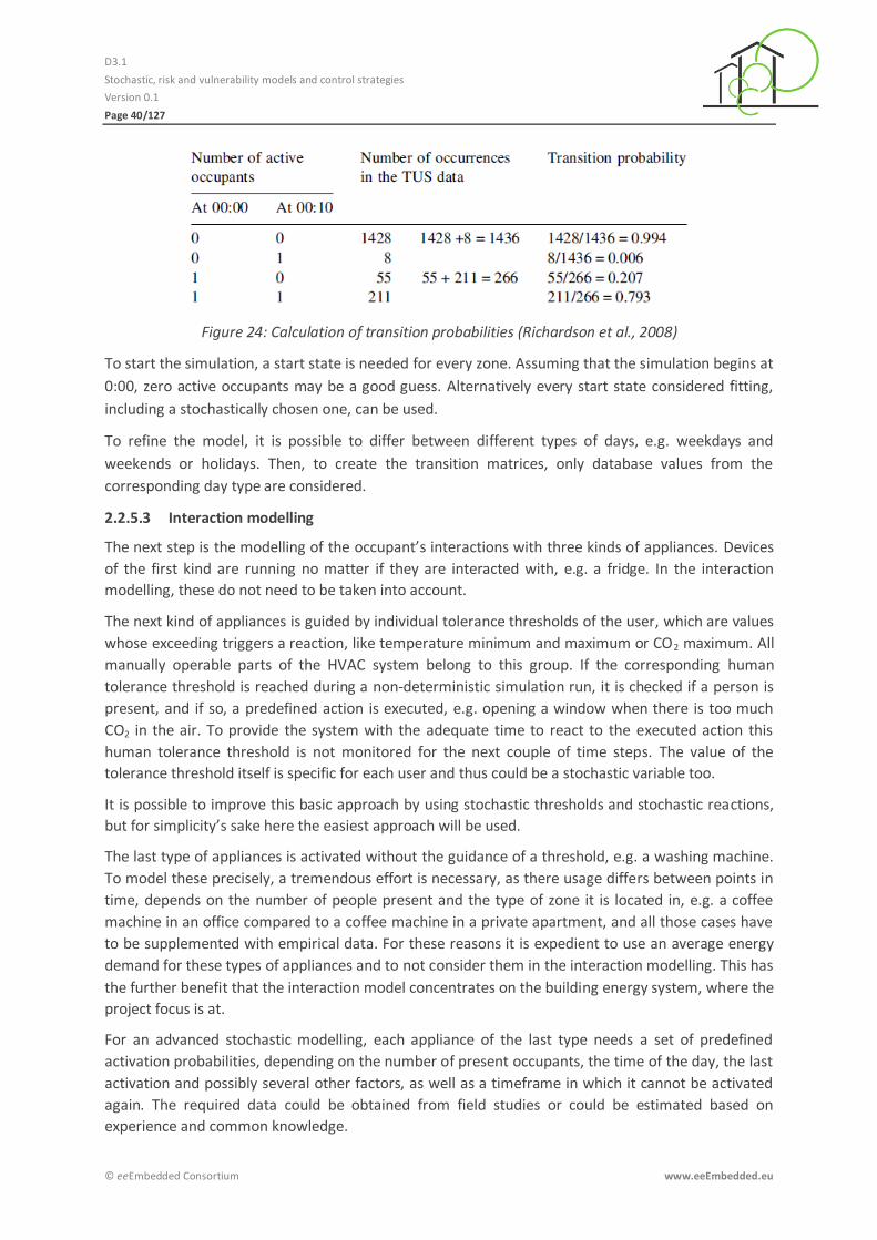
To get a transition probability between two states, one counts all occurrences of this transition in the

dataset at the given time step and divides it by the number of entries concerning the time of interest.

In Figure 23 and Figure 24, taken from (Richardson et al., 2008), one can see an example of a

transition matrix for a zone with a maximum of 1 occupant, as well as the calculations to obtain the

probabilities.

Figure 23: Example of a transition matrix (Richardson et al., 2008)

D3.1


Version 0.1

Page 40/127


Figure 24: Calculation of transition probabilities (Richardson et al., 2008)

To start the simulation, a start state is needed for every zone. Assuming that the simulation begins at

0:00, zero active occupants may be a good guess. Alternatively every start state considered fitting,

including a stochastically chosen one, can be used.

To refine the model, it is possible to differ between different types of days, e.g. weekdays and

weekends or holidays. Then, to create the transition matrices, only database values from the

corresponding day type are considered.

2.2.5.3 Interaction modelling

The next step is the modelling of the occupant’s interactions with three kinds of appliances. Devices

of the first kind are running no matter if they are interacted with, e.g. a fridge. In the interaction

modelling, these do not need to be taken into account.

The next kind of appliances is guided by individual tolerance thresholds of the user, which are values

whose exceeding triggers a reaction, like temperature minimum and maximum or CO2 maximum. All

manually operable parts of the HVAC system belong to this group. If the corresponding human

tolerance threshold is reached during a non-deterministic simulation run, it is checked if a person is

present, and if so, a predefined action is executed, e.g. opening a window when there is too much

CO2 in the air. To provide the system with the adequate time to react to the executed action this

human tolerance threshold is not monitored for the next couple of time steps. The value of the

tolerance threshold itself is specific for each user and thus could be a stochastic variable too.

It is possible to improve this basic approach by using stochastic thresholds and stochastic reactions,

but for simplicity’s sake here the easiest approach will be used.

The last type of appliances is activated without the guidance of a threshold, e.g. a washing machine.

To model these precisely, a tremendous effort is necessary, as there usage differs between points in

time, depends on the number of people present and the type of zone it is located in, e.g. a coffee

machine in an office compared to a coffee machine in a private apartment, and all those cases have

to be supplemented with empirical data. For these reasons it is expedient to use an average energy

demand for these types of appliances and to not consider them in the interaction modelling. This has

the further benefit that the interaction model concentrates on the building energy system, where the

project focus is at.

For an advanced stochastic modelling, each appliance of the last type needs a set of predefined

activation probabilities, depending on the number of present occupants, the time of the day, the last

activation and possibly several other factors, as well as a timeframe in which it cannot be activated

again. The required data could be obtained from field studies or could be estimated based on

experience and common knowledge.

D3.1


Version 0.1

Page 41/127


Regressor climate trend 2.2.6


Processing building lifecycle analysis commonly covers a period of about 30 to 50 years. Focussing on

the main drivers of the energy demand especially for heating and cooling purposes leads to the

climate or more specific to the climate change within the period under observation. A brief definition

of the term ‘climate’ is given in (Bernhofer, 2008) as the totality of all weather states including their

typical sequence and their daily and seasonable fluctuations which are possible at a certain location.

Following this definition, the climate is the result of processes within the atmosphere but also the

result of the interdependencies between continents, oceans, atmosphere and solar activity.

The analysis of climate and climate change needs a separation of the climate into the basic climate

(Bernhofer, 2008) elements with significant influence on building design and energy demand: (1)

temperature, (2) precipitation, (3) wind, (4) radiation balance, (5) potential evaporation, and (6)

climatic water balance. Climate elements are meteorological values characterising the climate as

single value or as combination of values. The first four mentioned climate elements have a

fundamental importance and will affect the building and energy system design. Besides the climate

elements, climate factors are identified and addressed as processes and states which cause, sustain

and modify the climate. Typical factors are solar radiation, height above sea level and the spread of

land and sea areas.

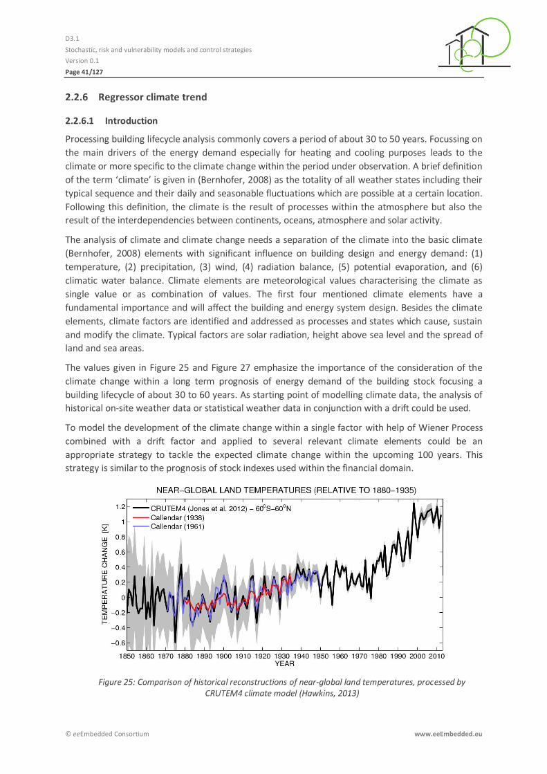
The values given in Figure 25 and Figure 27 emphasize the importance of the consideration of the

climate change within a long term prognosis of energy demand of the building stock focusing a

building lifecycle of about 30 to 60 years. As starting point of modelling climate data, the analysis of

historical on-site weather data or statistical weather data in conjunction with a drift could be used.

To model the development of the climate change within a single factor with help of Wiener Process

combined with a drift factor and applied to several relevant climate elements could be an

appropriate strategy to tackle the expected climate change within the upcoming 100 years. This

strategy is similar to the prognosis of stock indexes used within the financial domain.

Figure 25: Comparison of historical reconstructions of near-global land temperatures, processed by CRUTEM4 climate model (Hawkins, 2013)

D3.1


Version 0.1

Page 42/127


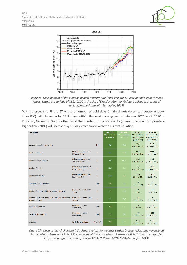
Figure 26: Development of the avarage annual temperature (thick line are 11-year-periode smooth mean values) within the periode of 1821-2100 in the city of Dresden (Germany); future values are results of

several prognosis models (Bernhofer, 2013)

With reference to Figure 27 e.g. the number of cold days (minimal outside air temperature lower

than 0°C) will decrease by 17.3 days within the next coming years between 2021 until 2050 in

Dresden, Germany. On the other hand the number of tropical nights (mean outside air temperature

higher than 20°C) will increase by 1.6 days compared with the current situation.

Figure 27: Mean values of characteristic climate values for weather station Dresden-Klotzsche – measured historical data between 1961-1990 compared with measured data between 1991-2010 and results of a

long term prognosis covering periods 2021-2050 and 2071-2100 (Bernhofer, 2013)

D3.1


Version 0.1

Page 43/127


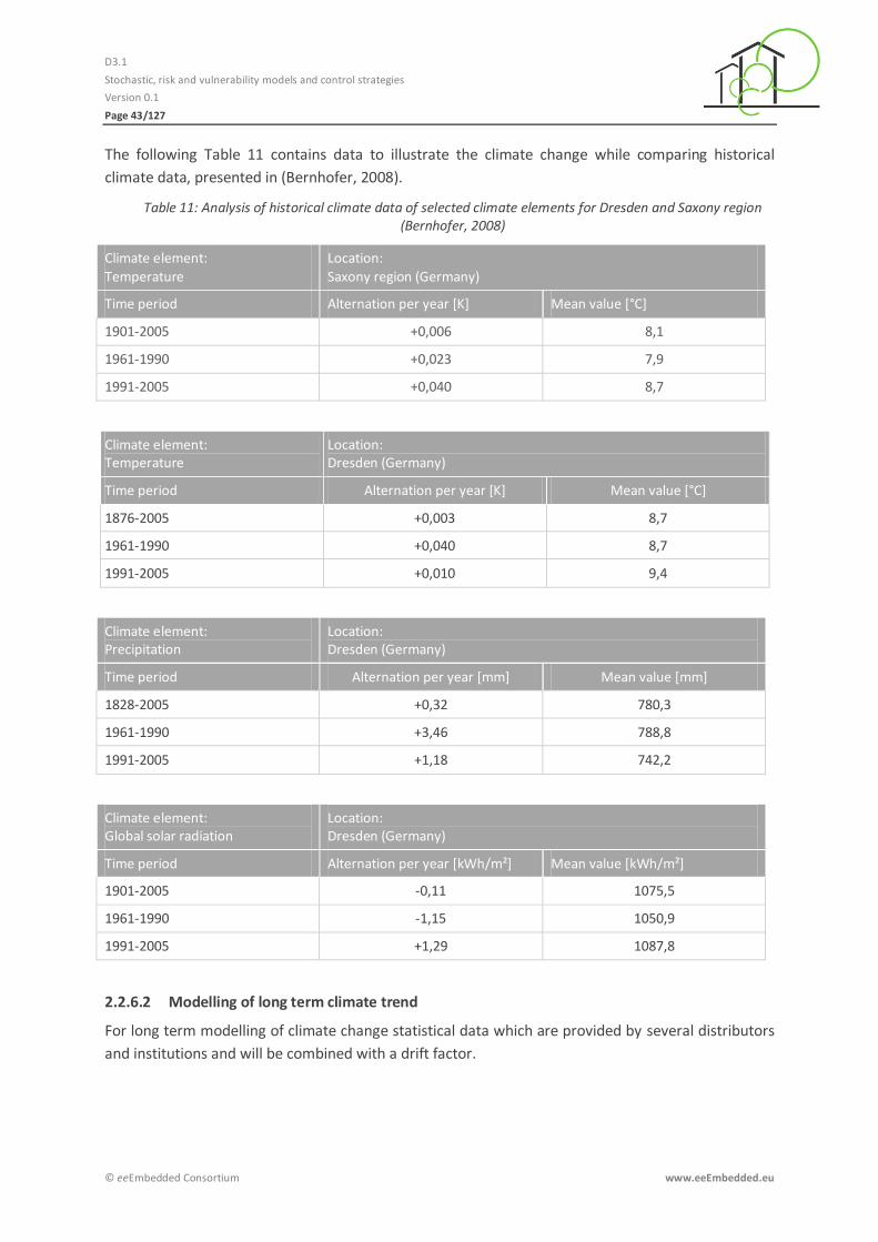
The following Table 11 contains data to illustrate the climate change while comparing historical

climate data, presented in (Bernhofer, 2008).

Table 11: Analysis of historical climate data of selected climate elements for Dresden and Saxony region (Bernhofer, 2008)

Climate element:

Temperature

Location:

Saxony region (Germany)

Time period Alternation per year [K] Mean value [°C]

1901-2005 +0,006 8,1

1961-1990 +0,023 7,9

1991-2005 +0,040 8,7

Climate element: Temperature

Location: Dresden (Germany)

Time period Alternation per year [K] Mean value [°C]

1876-2005 +0,003 8,7

1961-1990 +0,040 8,7

1991-2005 +0,010 9,4

Climate element: Precipitation


Time period Alternation per year [mm] Mean value [mm]

1828-2005 +0,32 780,3

1961-1990 +3,46 788,8

1991-2005 +1,18 742,2

Climate element: Global solar radiation


Time period Alternation per year [kWh/m²] Mean value [kWh/m²]

1901-2005 -0,11 1075,5

1961-1990 -1,15 1050,9

1991-2005 +1,29 1087,8

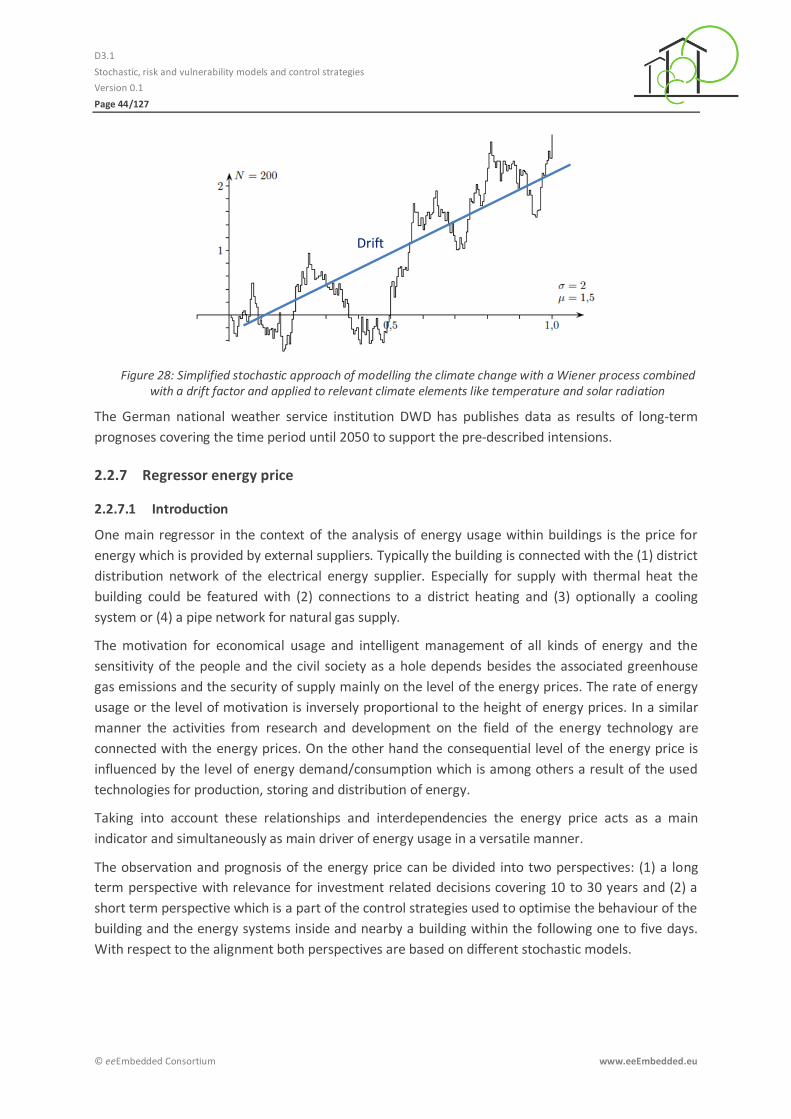
2.2.6.2 Modelling of long term climate trend

For long term modelling of climate change statistical data which are provided by several distributors

and institutions and will be combined with a drift factor.

D3.1


Version 0.1

Page 44/127


Figure 28: Simplified stochastic approach of modelling the climate change with a Wiener process combined with a drift factor and applied to relevant climate elements like temperature and solar radiation

The German national weather service institution DWD has publishes data as results of long-term

prognoses covering the time period until 2050 to support the pre-described intensions.

Regressor energy price 2.2.7


One main regressor in the context of the analysis of energy usage within buildings is the price for

energy which is provided by external suppliers. Typically the building is connected with the (1) district

distribution network of the electrical energy supplier. Especially for supply with thermal heat the

building could be featured with (2) connections to a district heating and (3) optionally a cooling

system or (4) a pipe network for natural gas supply.

The motivation for economical usage and intelligent management of all kinds of energy and the

sensitivity of the people and the civil society as a hole depends besides the associated greenhouse

gas emissions and the security of supply mainly on the level of the energy prices. The rate of energy

usage or the level of motivation is inversely proportional to the height of energy prices. In a similar

manner the activities from research and development on the field of the energy technology are

connected with the energy prices. On the other hand the consequential level of the energy price is

influenced by the level of energy demand/consumption which is among others a result of the used

technologies for production, storing and distribution of energy.

Taking into account these relationships and interdependencies the energy price acts as a main

indicator and simultaneously as main driver of energy usage in a versatile manner.

The observation and prognosis of the energy price can be divided into two perspectives: (1) a long

term perspective with relevance for investment related decisions covering 10 to 30 years and (2) a

short term perspective which is a part of the control strategies used to optimise the behaviour of the

building and the energy systems inside and nearby a building within the following one to five days.

With respect to the alignment both perspectives are based on different stochastic models.

Drift

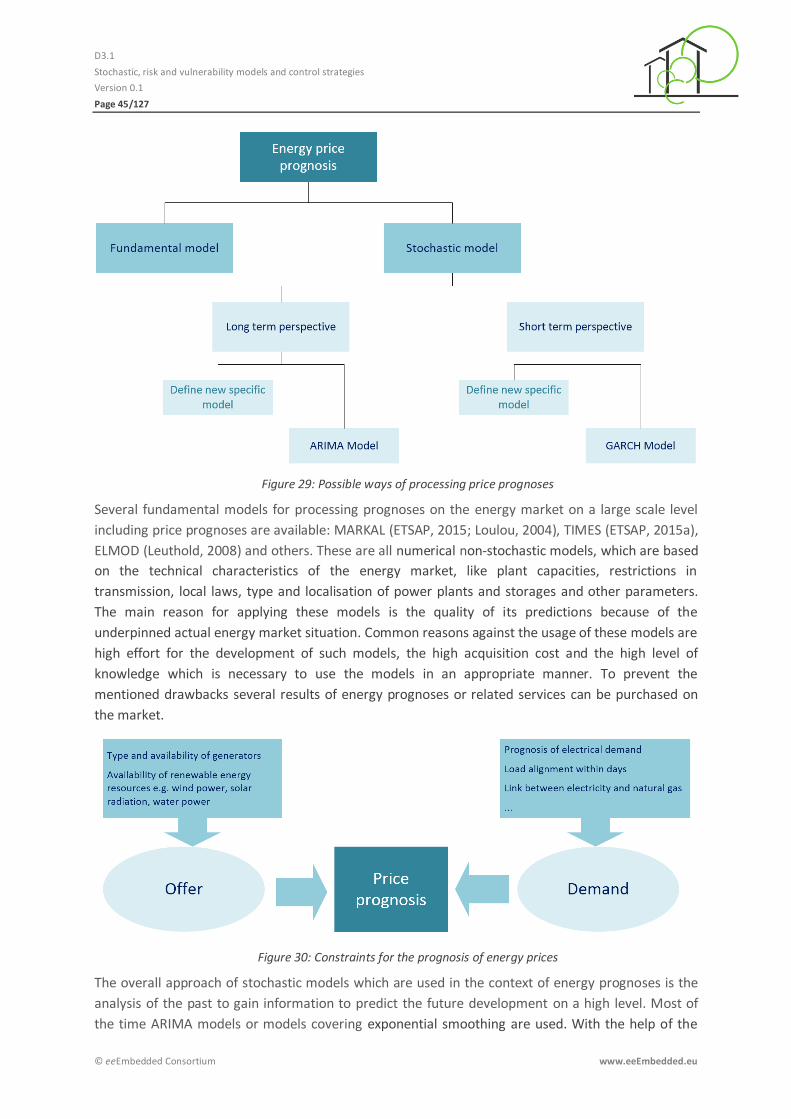
D3.1


Version 0.1

Page 45/127


Figure 29: Possible ways of processing price prognoses

Several fundamental models for processing prognoses on the energy market on a large scale level

including price prognoses are available: MARKAL (ETSAP, 2015; Loulou, 2004), TIMES (ETSAP, 2015a),

ELMOD (Leuthold, 2008) and others. These are all numerical non-stochastic models, which are based

on the technical characteristics of the energy market, like plant capacities, restrictions in

transmission, local laws, type and localisation of power plants and storages and other parameters.

The main reason for applying these models is the quality of its predictions because of the

underpinned actual energy market situation. Common reasons against the usage of these models are

high effort for the development of such models, the high acquisition cost and the high level of

knowledge which is necessary to use the models in an appropriate manner. To prevent the

mentioned drawbacks several results of energy prognoses or related services can be purchased on

the market.

Figure 30: Constraints for the prognosis of energy prices

The overall approach of stochastic models which are used in the context of energy prognoses is the

analysis of the past to gain information to predict the future development on a high level. Most of

the time ARIMA models or models covering exponential smoothing are used. With the help of the

D3.1


Version 0.1

Page 46/127


forecast approach the best fitting parameters for a given time series will be found to predict the

future values including confidence intervals. These models are easy to use and when using pre-

configured software packages for processing forecast, the model of a given class which fits best will

be found. As main argument against the usage of stochastic models in this context could be

mentioned that the processed analysis is not the natural way of representing dependencies.

There are several data related issues which have to be discussed when applying prognoses in general

and stochastic approaches in specific to the target of depending on the target of forecasting energy

prices. Regarding the time resolution the mentioned long term prognoses could be processed on

hourly or daily basis depending on the level of detail for modelling the energy systems and the

energy demand when covering a forecast period of 10 to 30 years or more.

According to the character of the long term prognoses the results are covering a broad confidence

interval. Applying long term prognoses according to a single location like a building site in

conjunction with a wide prognosis period several uncertainties with high impact on the results are

arising. Typical factors - partly with strong relation to a certain country or an administrative region -

in that sense are politically, financially (e.g. tax fees) and technologically driven boundary conditions.

The regionalisation of the processed results while focussing on a certain location is a mayor issue

when using these data too. While making design related decisions about the conjunction with the

building envelop and the type of energy systems, the overall long-term trend of the energy price acts

as the main factor which has to be observed.

2.2.7.2 Indices

Appropriate indices are available to monitor the rate of energy related exchange activities, e.g. the

wholesale price for electrical energy named as Physical Electricity Index (Phelix) and its derivatives

available for Germany and Austria monitored on the European Power Exchange (EPEX SPOT) in Paris

which acts as reference index. NetConnect Germany provides the price index NCG.

Figure 31: Example of Phelix index and derivatives (wholesaling price for electrical energy) between June 2013 and June 2015 (ISPEX, 2015)

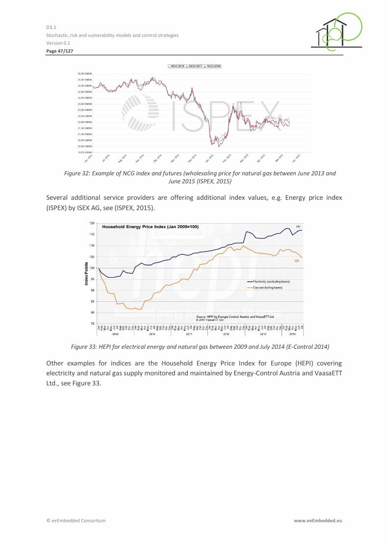
D3.1


Version 0.1

Page 47/127


Figure 32: Example of NCG index and futures (wholesaling price for natural gas between June 2013 and June 2015 (ISPEX, 2015)

Several additional service providers are offering additional index values, e.g. Energy price index

(ISPEX) by ISEX AG, see (ISPEX, 2015).

Figure 33: HEPI for electrical energy and natural gas between 2009 and July 2014 (E-Control 2014)

Other examples for indices are the Household Energy Price Index for Europe (HEPI) covering

electricity and natural gas supply monitored and maintained by Energy-Control Austria and VaasaETT

Ltd., see Figure 33.

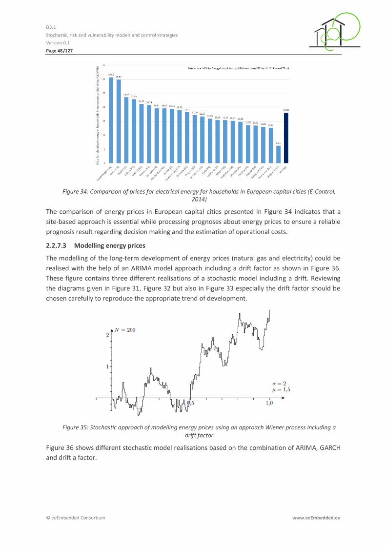
D3.1


Version 0.1

Page 48/127


Figure 34: Comparison of prices for electrical energy for households in European capital cities (E-Control, 2014)

The comparison of energy prices in European capital cities presented in Figure 34 indicates that a

site-based approach is essential while processing prognoses about energy prices to ensure a reliable

prognosis result regarding decision making and the estimation of operational costs.

2.2.7.3 Modelling energy prices

The modelling of the long-term development of energy prices (natural gas and electricity) could be

realised with the help of an ARIMA model approach including a drift factor as shown in Figure 36.

These figure contains three different realisations of a stochastic model including a drift. Reviewing

the diagrams given in Figure 31, Figure 32 but also in Figure 33 especially the drift factor should be

chosen carefully to reproduce the appropriate trend of development.

Figure 35: Stochastic approach of modelling energy prices using an approach Wiener process including a drift factor

Figure 36 shows different stochastic model realisations based on the combination of ARIMA, GARCH

and drift a factor.

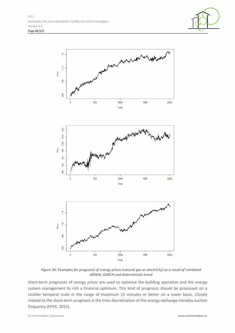
D3.1


Version 0.1

Page 49/127


Figure 36: Examples for prognosis of energy prices (natural gas or electricity) as a result of combined ARIMA, GARCH und deterministic trend

Short-term prognoses of energy prices are used to optimise the building operation and the energy

system management to rich a financial optimum. This kind of prognosis should be processed on a

smaller temporal scale in the range of maximum 15 minutes or better on a lower basis. Closely

related to the short-term prognosis is the time discretisation of the energy exchange intraday auction

frequency (EPEX, 2015).

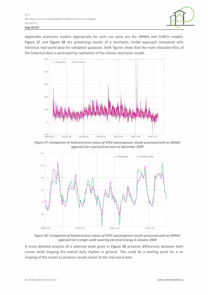
D3.1


Version 0.1

Page 50/127


Applicable stochastic models appropriate for such use cases are the ARIMA and GARCH models.

Figure 37 and Figure 38 are presenting results of a stochastic model approach compared with

historical real-world data for validation purposes. Both figures show that the main characteristics of

the historical data is portrayed by realisation of the chosen stochastic model.

Figure 37: Comparison of historical price values of EPEX and prognosis results processed with an ARIMA approach for a period from June to December 2009

Figure 38: Comparison of historical price values of EPEX and prognosis results processed with an ARIMA approach for a single week covering electrical energy in January 2009

A more detailed analysis of a selected week given in Figure 38 presents differences between both

curves while keeping the overall daily rhythm in general. This could be a starting point for a re-

shaping of the model to produce results closer to the real-word data.

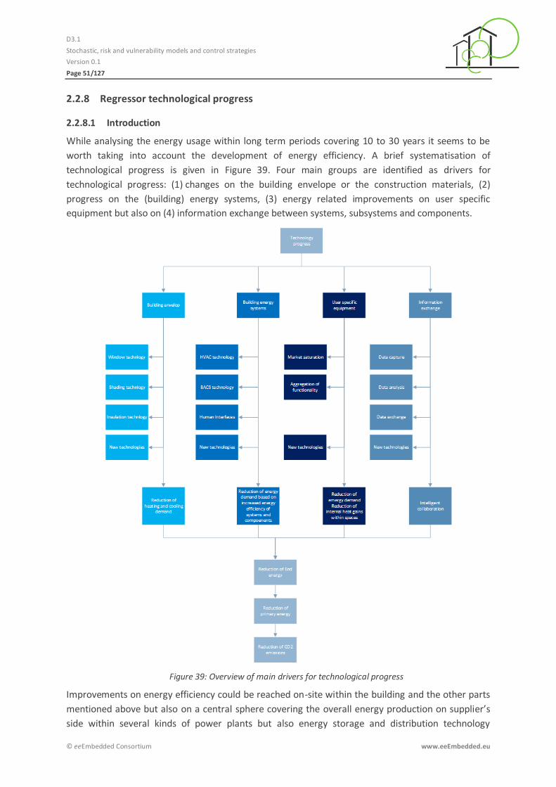
D3.1


Version 0.1

Page 51/127


Regressor technological progress 2.2.8


While analysing the energy usage within long term periods covering 10 to 30 years it seems to be

worth taking into account the development of energy efficiency. A brief systematisation of

technological progress is given in Figure 39. Four main groups are identified as drivers for

technological progress: (1) changes on the building envelope or the construction materials, (2)

progress on the (building) energy systems, (3) energy related improvements on user specific

equipment but also on (4) information exchange between systems, subsystems and components.

Figure 39: Overview of main drivers for technological progress

Improvements on energy efficiency could be reached on-site within the building and the other parts

mentioned above but also on a central sphere covering the overall energy production on supplier’s

side within several kinds of power plants but also energy storage and distribution technology

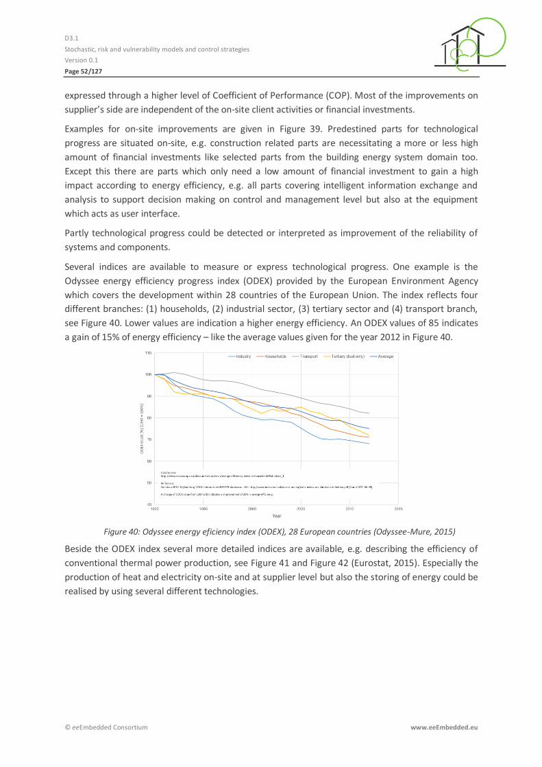
D3.1


Version 0.1

Page 52/127


expressed through a higher level of Coefficient of Performance (COP). Most of the improvements on

supplier’s side are independent of the on-site client activities or financial investments.

Examples for on-site improvements are given in Figure 39. Predestined parts for technological

progress are situated on-site, e.g. construction related parts are necessitating a more or less high

amount of financial investments like selected parts from the building energy system domain too.

Except this there are parts which only need a low amount of financial investment to gain a high

impact according to energy efficiency, e.g. all parts covering intelligent information exchange and

analysis to support decision making on control and management level but also at the equipment

which acts as user interface.

Partly technological progress could be detected or interpreted as improvement of the reliability of

systems and components.

Several indices are available to measure or express technological progress. One example is the

Odyssee energy efficiency progress index (ODEX) provided by the European Environment Agency

which covers the development within 28 countries of the European Union. The index reflects four

different branches: (1) households, (2) industrial sector, (3) tertiary sector and (4) transport branch,

see Figure 40. Lower values are indication a higher energy efficiency. An ODEX values of 85 indicates

a gain of 15% of energy efficiency – like the average values given for the year 2012 in Figure 40.

Figure 40: Odyssee energy eficiency index (ODEX), 28 European countries (Odyssee-Mure, 2015)

Beside the ODEX index several more detailed indices are available, e.g. describing the efficiency of

conventional thermal power production, see Figure 41 and Figure 42 (Eurostat, 2015). Especially the

production of heat and electricity on-site and at supplier level but also the storing of energy could be

realised by using several different technologies.

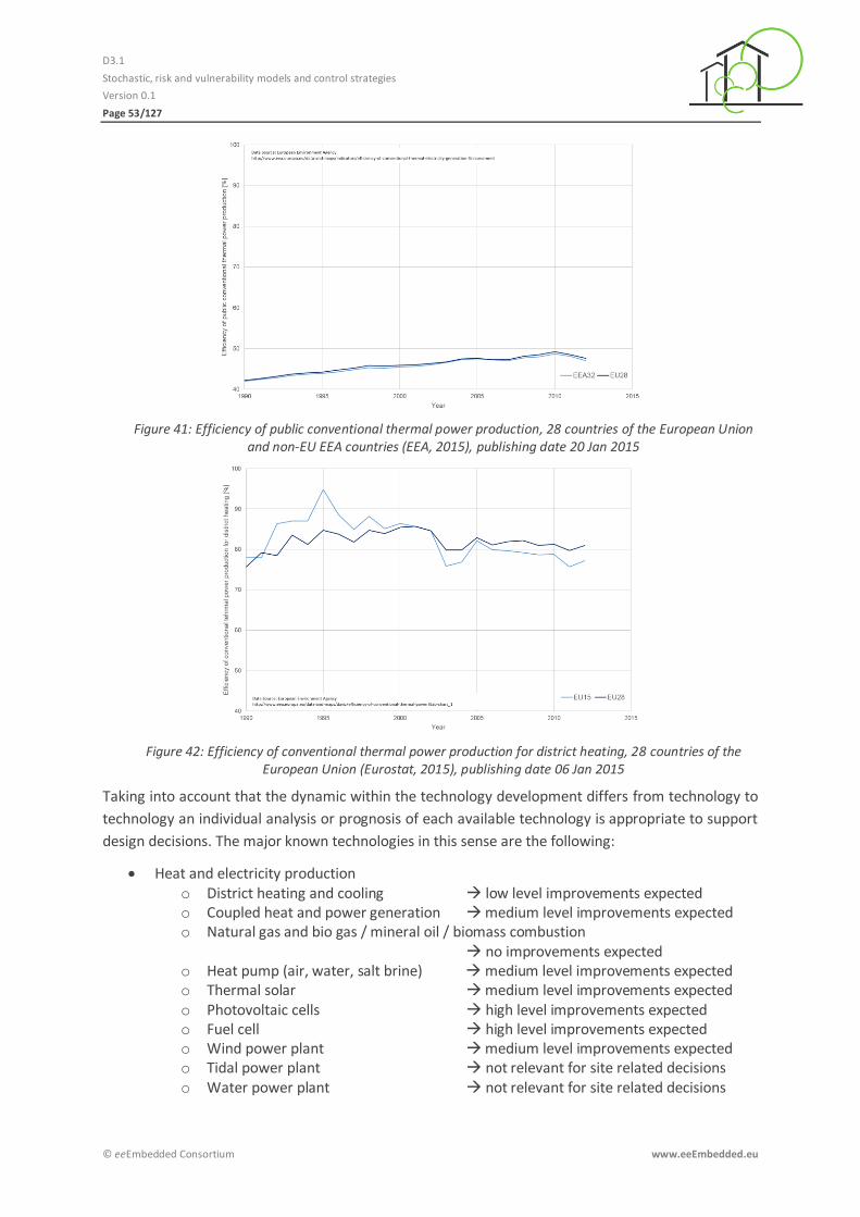
D3.1


Version 0.1

Page 53/127


Figure 41: Efficiency of public conventional thermal power production, 28 countries of the European Union and non-EU EEA countries (EEA, 2015), publishing date 20 Jan 2015

Figure 42: Efficiency of conventional thermal power production for district heating, 28 countries of the European Union (Eurostat, 2015), publishing date 06 Jan 2015

Taking into account that the dynamic within the technology development differs from technology to

technology an individual analysis or prognosis of each available technology is appropriate to support

design decisions. The major known technologies in this sense are the following:

Heat and electricity production o District heating and cooling low level improvements expected o Coupled heat and power generation medium level improvements expected o Natural gas and bio gas / mineral oil / biomass combustion

no improvements expected o Heat pump (air, water, salt brine) medium level improvements expected o Thermal solar medium level improvements expected o Photovoltaic cells high level improvements expected o Fuel cell high level improvements expected o Wind power plant medium level improvements expected o Tidal power plant not relevant for site related decisions o Water power plant not relevant for site related decisions

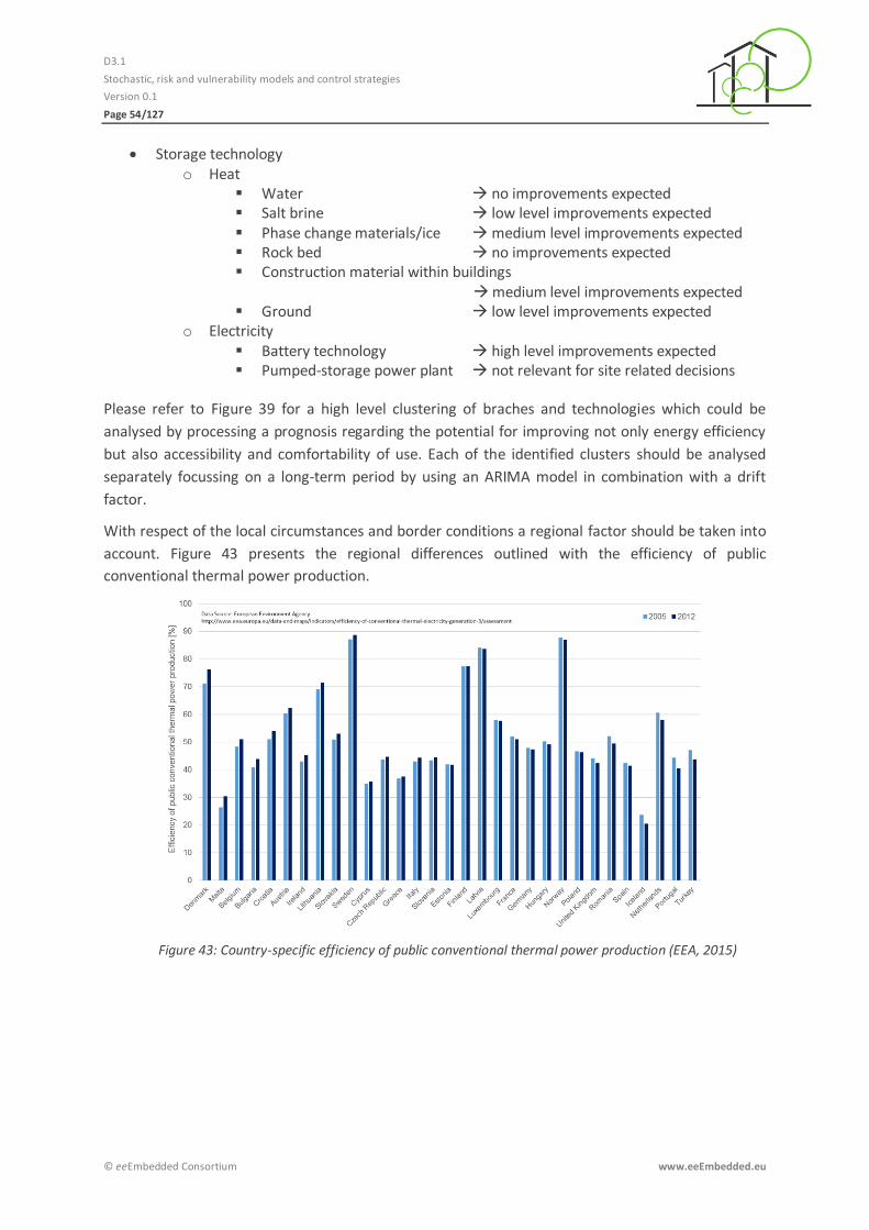
D3.1


Version 0.1

Page 54/127


Storage technology o Heat

Water no improvements expected Salt brine low level improvements expected Phase change materials/ice medium level improvements expected Rock bed no improvements expected Construction material within buildings

medium level improvements expected Ground low level improvements expected

o Electricity Battery technology high level improvements expected Pumped-storage power plant not relevant for site related decisions

Please refer to Figure 39 for a high level clustering of braches and technologies which could be

analysed by processing a prognosis regarding the potential for improving not only energy efficiency

but also accessibility and comfortability of use. Each of the identified clusters should be analysed

separately focussing on a long-term period by using an ARIMA model in combination with a drift

factor.

With respect of the local circumstances and border conditions a regional factor should be taken into

account. Figure 43 presents the regional differences outlined with the efficiency of public

conventional thermal power production.

Figure 43: Country-specific efficiency of public conventional thermal power production (EEA, 2015)

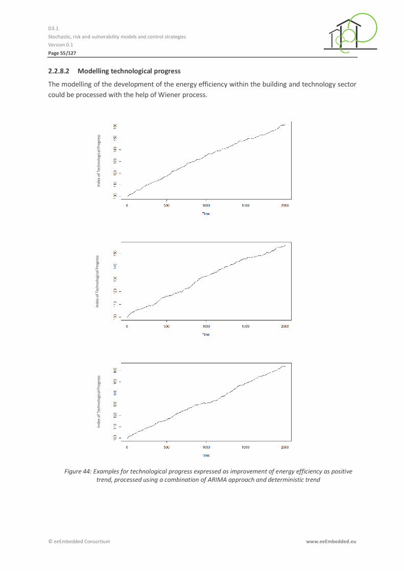
D3.1


Version 0.1

Page 55/127


2.2.8.2 Modelling technological progress

The modelling of the development of the energy efficiency within the building and technology sector

could be processed with the help of Wiener process.

Figure 44: Examples for technological progress expressed as improvement of energy efficiency as positive trend, processed using a combination of ARIMA approach and deterministic trend

Ind

ex o

f Te

chn

olo

gica

l Pro

gres

s In

dex

of

Tech

no

logi

cal P

rogr

ess

Ind

ex o

f Te

chn

olo

gica

l Pro

gres

s

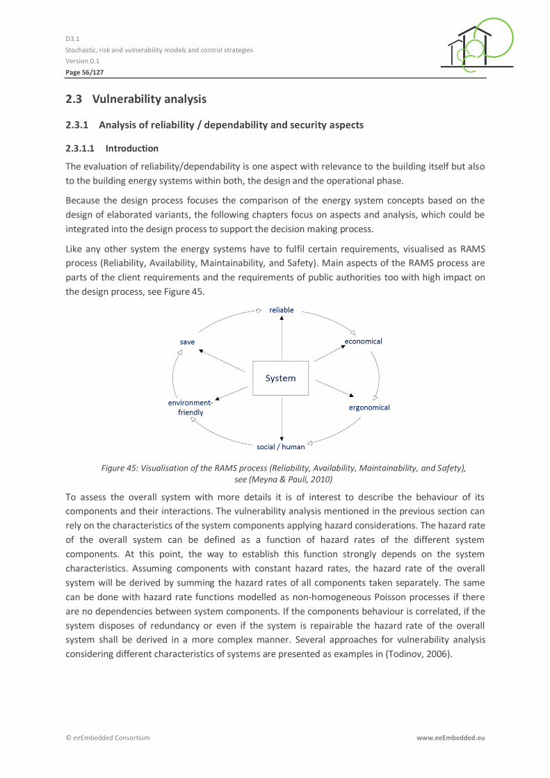
D3.1


Version 0.1

Page 56/127


2.3 Vulnerability analysis

Analysis of reliability / dependability and security aspects 2.3.1


The evaluation of reliability/dependability is one aspect with relevance to the building itself but also

to the building energy systems within both, the design and the operational phase.

Because the design process focuses the comparison of the energy system concepts based on the

design of elaborated variants, the following chapters focus on aspects and analysis, which could be

integrated into the design process to support the decision making process.

Like any other system the energy systems have to fulfil certain requirements, visualised as RAMS

process (Reliability, Availability, Maintainability, and Safety). Main aspects of the RAMS process are

parts of the client requirements and the requirements of public authorities too with high impact on

the design process, see Figure 45.

Figure 45: Visualisation of the RAMS process (Reliability, Availability, Maintainability, and Safety), see (Meyna & Pauli, 2010)

To assess the overall system with more details it is of interest to describe the behaviour of its

components and their interactions. The vulnerability analysis mentioned in the previous section can

rely on the characteristics of the system components applying hazard considerations. The hazard rate

of the overall system can be defined as a function of hazard rates of the different system

components. At this point, the way to establish this function strongly depends on the system

characteristics. Assuming components with constant hazard rates, the hazard rate of the overall

system will be derived by summing the hazard rates of all components taken separately. The same

can be done with hazard rate functions modelled as non-homogeneous Poisson processes if there

are no dependencies between system components. If the components behaviour is correlated, if the

system disposes of redundancy or even if the system is repairable the hazard rate of the overall

system shall be derived in a more complex manner. Several approaches for vulnerability analysis

considering different characteristics of systems are presented as examples in (Todinov, 2006).

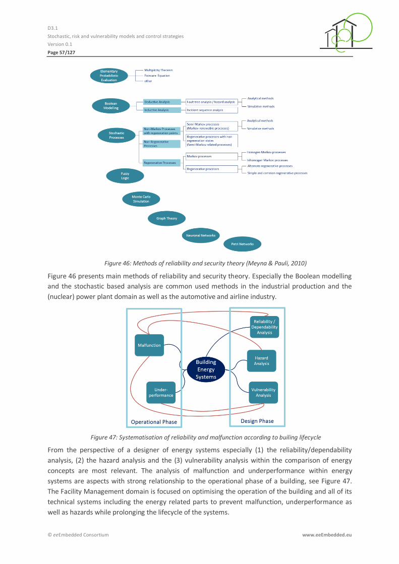
D3.1


Version 0.1

Page 57/127


Figure 46: Methods of reliability and security theory (Meyna & Pauli, 2010)

Figure 46 presents main methods of reliability and security theory. Especially the Boolean modelling

and the stochastic based analysis are common used methods in the industrial production and the

(nuclear) power plant domain as well as the automotive and airline industry.

Figure 47: Systematisation of reliability and malfunction according to builing lifecycle

From the perspective of a designer of energy systems especially (1) the reliability/dependability

analysis, (2) the hazard analysis and the (3) vulnerability analysis within the comparison of energy

concepts are most relevant. The analysis of malfunction and underperformance within energy

systems are aspects with strong relationship to the operational phase of a building, see Figure 47.

The Facility Management domain is focused on optimising the operation of the building and all of its

technical systems including the energy related parts to prevent malfunction, underperformance as

well as hazards while prolonging the lifecycle of the systems.

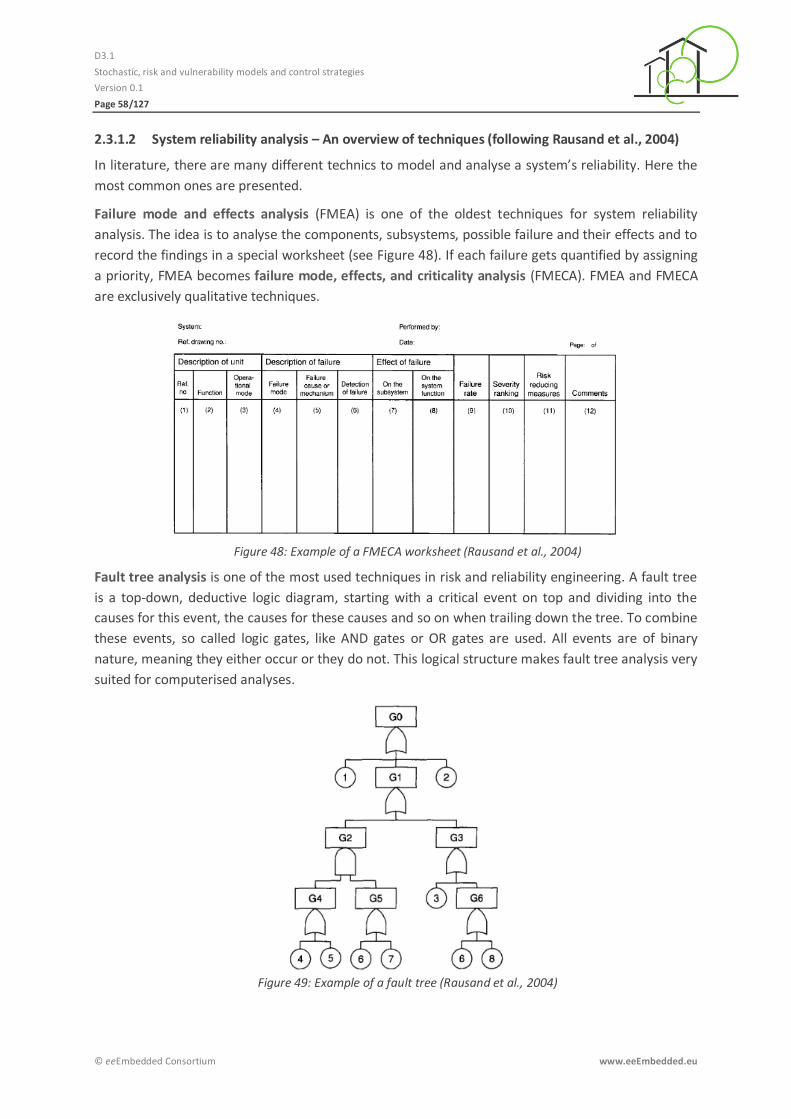
D3.1


Version 0.1

Page 58/127


2.3.1.2 System reliability analysis – An overview of techniques (following Rausand et al., 2004)

In literature, there are many different technics to model and analyse a system’s reliability. Here the

most common ones are presented.

Failure mode and effects analysis (FMEA) is one of the oldest techniques for system reliability

analysis. The idea is to analyse the components, subsystems, possible failure and their effects and to

record the findings in a special worksheet (see Figure 48). If each failure gets quantified by assigning

a priority, FMEA becomes failure mode, effects, and criticality analysis (FMECA). FMEA and FMECA

are exclusively qualitative techniques.

Figure 48: Example of a FMECA worksheet (Rausand et al., 2004)

Fault tree analysis is one of the most used techniques in risk and reliability engineering. A fault tree

is a top-down, deductive logic diagram, starting with a critical event on top and dividing into the

causes for this event, the causes for these causes and so on when trailing down the tree. To combine

these events, so called logic gates, like AND gates or OR gates are used. All events are of binary

nature, meaning they either occur or they do not. This logical structure makes fault tree analysis very

suited for computerised analyses.

Figure 49: Example of a fault tree (Rausand et al., 2004)

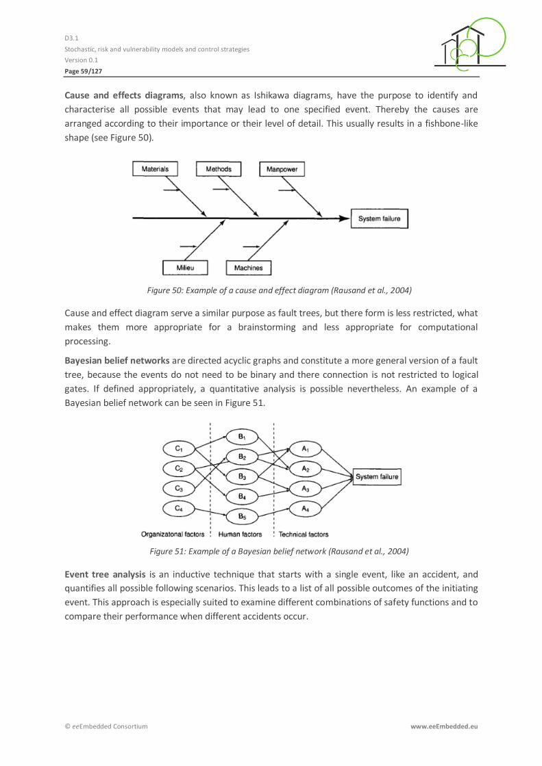
D3.1


Version 0.1

Page 59/127


Cause and effects diagrams, also known as Ishikawa diagrams, have the purpose to identify and

characterise all possible events that may lead to one specified event. Thereby the causes are

arranged according to their importance or their level of detail. This usually results in a fishbone-like

shape (see Figure 50).

Figure 50: Example of a cause and effect diagram (Rausand et al., 2004)

Cause and effect diagram serve a similar purpose as fault trees, but there form is less restricted, what

makes them more appropriate for a brainstorming and less appropriate for computational

processing.

Bayesian belief networks are directed acyclic graphs and constitute a more general version of a fault

tree, because the events do not need to be binary and there connection is not restricted to logical

gates. If defined appropriately, a quantitative analysis is possible nevertheless. An example of a

Bayesian belief network can be seen in Figure 51.

Figure 51: Example of a Bayesian belief network (Rausand et al., 2004)

Event tree analysis is an inductive technique that starts with a single event, like an accident, and

quantifies all possible following scenarios. This leads to a list of all possible outcomes of the initiating

event. This approach is especially suited to examine different combinations of safety functions and to

compare their performance when different accidents occur.

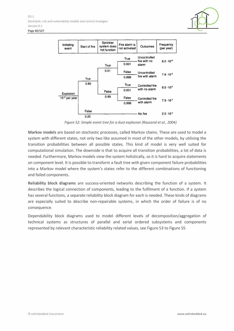
D3.1


Version 0.1

Page 60/127


Figure 52: Simple event tree for a dust explosion (Rausand et al., 2004)

Markov models are based on stochastic processes, called Markov chains. These are used to model a

system with different states, not only two like assumed in most of the other models, by utilising the

transition probabilities between all possible states. This kind of model is very well suited for

computational simulation. The downside is that to acquire all transition probabilities, a lot of data is

needed. Furthermore, Markov models view the system holistically, so it is hard to acquire statements

on component level. It is possible to transform a fault tree with given component failure probabilities

into a Markov model where the system’s states refer to the different combinations of functioning

and failed components.

Reliability block diagrams are success-oriented networks describing the function of a system. It

describes the logical connection of components, leading to the fulfilment of a function. If a system

has several functions, a separate reliability block diagram for each is needed. These kinds of diagrams

are especially suited to describe non-repairable systems, in which the order of failure is of no

consequence.

Dependability block diagrams used to model different levels of decomposition/aggregation of

technical systems as structures of parallel and serial ordered subsystems and components

represented by relevant characteristic reliability related values, see Figure 53 to Figure 55

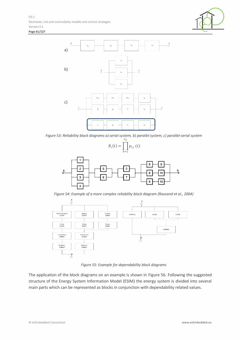
D3.1


Version 0.1

Page 61/127


Figure 53: Reliability block diagrams a) serial system, b) parallel system, c) parallel-serial system

∏

Figure 54: Example of a more complex reliability block diagram (Rausand et al., 2004)

Figure 55: Example for dependability block diagrams

The application of the block diagrams on an example is shown in Figure 56. Following the suggested

structure of the Energy System Information Model (ESIM) the energy system is divided into several

main parts which can be represented as blocks in conjunction with dependability related values.

b)

c)

a)

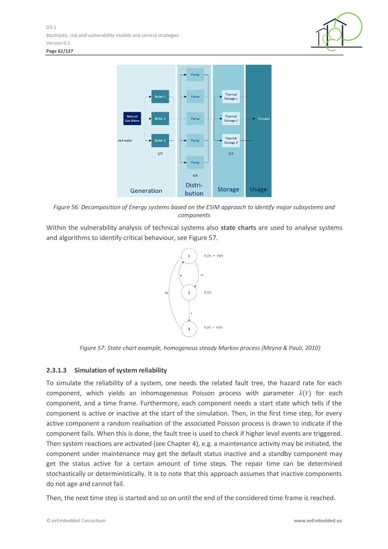
D3.1


Version 0.1

Page 62/127


Figure 56: Decomposition of Energy systems based on the ESIM approach to identify major subsystems and components

Within the vulnerability analysis of technical systems also state charts are used to analyse systems

and algorithms to identify critical behaviour, see Figure 57.

Figure 57: State chart example, homogenous steady Markov process (Meyna & Pauli, 2010)

2.3.1.3 Simulation of system reliability

To simulate the reliability of a system, one needs the related fault tree, the hazard rate for each

component, which yields an inhomogeneous Poisson process with parameter for each

component, and a time frame. Furthermore, each component needs a start state which tells if the

component is active or inactive at the start of the simulation. Then, in the first time step, for every

active component a random realisation of the associated Poisson process is drawn to indicate if the

component fails. When this is done, the fault tree is used to check if higher level events are triggered.

Then system reactions are activated (see Chapter 4), e.g. a maintenance activity may be initiated, the

component under maintenance may get the default status inactive and a standby component may

get the status active for a certain amount of time steps. The repair time can be determined

stochastically or deterministically. It is to note that this approach assumes that inactive components

do not age and cannot fail.

Then, the next time step is started and so on until the end of the considered time frame is reached.

D3.1


Version 0.1

Page 63/127


If a component has a non-constant hazard rate, it may be advisable to reset after it got repaired,

e.g. to the beginning of the useful life region (see Figure 58).

In most cases the goal is to derive KPIs, e.g. described in Chapter 2.3.2, referring to the failure of the

whole system, which is the top event of the corresponding fault tree, so at least these points in time

at which the system fails have to be stored during simulation. As failure of the system is most often

an event with very small probability, the simulation has to be repeated several times before

statistical statements can be claimed.

2.3.1.4 Optimisation of reliability/dependability within the design process

There are several approaches available for enhancing dependability and robustness within the design

phase (Meyna & Pauli, 2010):

Simplification enhance dependability through reduction of complexity

Marginal importance reduction of importance of an single component or sub-system concerning the failure probability of the hole system; identify the components within a system which are most important for the survival or failure-free operation of the system

Derating / permanent load reduction Reduction of the load level of relevant components to enlarge the lifetime or to reduce the probability of failure

Redundancy multiply the existence of components with an high importance for the survival or failure-free operation of the system

The pre-mentioned aspects can be taken into consideration when designing technical systems. The

integration of these points into the comparison and analysis the energy systems can provide

important inputs into the decision making domain within the design process.

Several techniques and methods are available for system conception and system evaluation:

Reliability model

Reliability allocation

Reliability prognosis Failure type , failure effect, criticality analysis

Tolerance analysis

System / subsystem / component choice

Especially thermal energy systems are exposed to varying operational conditions within the

operation phase. With respect to this conditions several evaluation methods are available to rate the

reliability/dependability of technical systems, subsystems and components mostly used on

manufacturers side but not within the design phase of a building:

Temperature dependence according to ARRHENIUS

Temperature-humidity dependence according to EYRING

Mechanical load according to WÖHLER

Temperature-change according to COFFIN-MANSON

Compared with the industry production and the electronic industry there is a very small data base

available which provide information to reliability/dependability. The manufacturers of components

used inside of energy systems are mostly not forced by law or other standards to publish a broad

D3.1


Version 0.1

Page 64/127


variety of information about reliability/dependability which could be used within an analysis. There

are a small number of data resources/handbooks available to predict dependability provided by the

electronic/semiconductor industry as well as military departments and the large scale production

industry, see (Meyna & Pauli, 2010):

Bell

SAE

Siemens (SN 29500)

ESReDA

MIL-HDBK217

Union Technique de l'Electricite (RDF 2000)

EPRD-97

NPRD-95 / 2011

The information given within these resources cover failure rates for certain technical components

and systems. The failure rates are based on several different models, see (Meyna & Pauli, 2010):

Constant failure rate o Time dependent linear failure rate o Time dependent linear increasing failure rate o Time dependent linear decreasing failure rate o Linear bath tube failure rate model

Common failure rate model

Average failure rate model

Timely variable failure rate

2.3.1.5 Key figures

Several Key Performance Indicators within the reliability/dependability are described below.

MTBF

One of the major key figures in the reliability/dependability analysis is the Mean Time Between

Failures (MTBF). This value describes the expected average operational time between the

occurrences of two consecutive failures events of a maintained technical unit. MTBF is used as Key

Performance Indicator for technical components or systems. Within the analysis of design concepts

this value could be used as key figure for evaluation purposes to compare concepts or components.

MTBF has a strong relationship to the maintenance concept and the FM domain.

MTTF

The abbreviation MTTF stands for Mean Time to Failure. This value describes the expected average

life time of a non-maintained technical unit. MTBF is used as Key Performance Indicator for technical

components or systems too and could be used in general to compare components or system

concepts.

MTTR

The abbreviation MTTR stands for Mean Time to Repair or Mean Time to Recover. This value

describes the expected average time for maintenance after an occurrence of a failure. MTTR is used

as Key Performance Indicator for maintenance planning in the FM domain.

D3.1


Version 0.1

Page 65/127


Availability

The availability A of a system is calculated based on the pre-mentioned values in the following

manner:

Energy consumption or production assigned to systems, subsystems, components

Especially within the analysis of malfunction and underperformance of an energy system the

difference between measured and expected energy consumption/production rate and the COP of

several components and systems can be used as indicator to detect suboptimal operational

behaviour of the technical systems and control algorithms.

2.3.1.6 Workflow

The overall workflow within the analysis covers the following steps:

1. Formulation of requirement/to-be state regarding each system, subsystem and component covering the following main topics

a. (Energy) performance b. Availability c. Reliability

2. Identification of values which are used as indicators describing the state implementation of the monitoring system (e.g. measurement equipment, maintenance data)

3. Generation of KPI expressing malfunction and/or underperformance

Prognosis of system downtime

Analysis of the applicability of the process for estimating malfunction and underperformance

o Based on discrete values as process results o Repeated Simulation of the stochastic process o Extraction of probability distributions

The analysis is based on investigation and elaboration of relevant

Inputs

Parameters

Border conditions

Restrictions in usage

The analysis has to check which modifications or combinations/superimpositions are needed to

produce reliable outputs.

Regressor reliability 2.3.2


Following the definition of the Institute of Electrical and Electronics Engineers (IEEE), reliability is “the

ability of a system or component to perform its required functions under stated conditions for a

specified period of time”, see (Verma et al., 2010).

There are four major aspects in this definition:

D3.1


Version 0.1

Page 66/127


- Ability refers to the likelihood that the system or component will work as expected and is therefore expressed by a number between 0 and 1

- Required function needs to be specified exactly and is the criterion reliability is measured against

- Specified period of time: A statement about reliability has only sense when restricted to a time frame

- Stated conditions include air pressure, temperature, humidity, etc. and may largely effect the reliability of a system or component

In eeEmbedded the working conditions will be assumed to be in an acceptable range. The reason for

this simplification is that a reliability simulation under different working conditions would need a

much larger data base, and the data situation concerning reliability in building engineering is already

quite limited.

2.3.2.2 Mathematical definition

To define reliability mathematically, for each component we have a random variable with a

distribution , describing the “time to first failure”. Then the reliability states the probability that

the component is still working correctly at an arbitrary point in time :

Now the hazard rate, which gives the average number of failure per unit of time is defined using the

probability density of , which is the derivative of with respect to the time:

By solving the resulting differential equation, one derives the following representation of :

{ ∫

}

2.3.2.3 Failure of components

To model reliability in eeEmbedded, the hazard rate for every component is needed. That is

realisable by either having access to the hazard rate directly, or by having information about and

its distribution , as depends only on the distribution of .

In reality, many components have a bath-tube shaped hazard curve (Figure 58).

Following (Verma et al., 2010), the three regions are called

1) Early failure region 2) Useful life region 3) Wear-out region

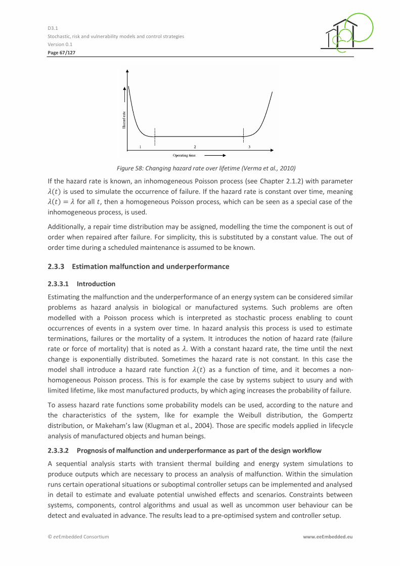
D3.1


Version 0.1

Page 67/127


Figure 58: Changing hazard rate over lifetime (Verma et al., 2010)

If the hazard rate is known, an inhomogeneous Poisson process (see Chapter 2.1.2) with parameter

is used to simulate the occurrence of failure. If the hazard rate is constant over time, meaning

for all , then a homogeneous Poisson process, which can be seen as a special case of the

inhomogeneous process, is used.

Additionally, a repair time distribution may be assigned, modelling the time the component is out of

order when repaired after failure. For simplicity, this is substituted by a constant value. The out of

order time during a scheduled maintenance is assumed to be known.

Estimation malfunction and underperformance 2.3.3


Estimating the malfunction and the underperformance of an energy system can be considered similar

problems as hazard analysis in biological or manufactured systems. Such problems are often

modelled with a Poisson process which is interpreted as stochastic process enabling to count

occurrences of events in a system over time. In hazard analysis this process is used to estimate

terminations, failures or the mortality of a system. It introduces the notion of hazard rate (failure

rate or force of mortality) that is noted as . With a constant hazard rate, the time until the next

change is exponentially distributed. Sometimes the hazard rate is not constant. In this case the

model shall introduce a hazard rate function as a function of time, and it becomes a non-

homogeneous Poisson process. This is for example the case by systems subject to usury and with

limited lifetime, like most manufactured products, by which aging increases the probability of failure.

To assess hazard rate functions some probability models can be used, according to the nature and

the characteristics of the system, like for example the Weibull distribution, the Gompertz

distribution, or Makeham’s law (Klugman et al., 2004). Those are specific models applied in lifecycle

analysis of manufactured objects and human beings.

2.3.3.2 Prognosis of malfunction and underperformance as part of the design workflow

A sequential analysis starts with transient thermal building and energy system simulations to

produce outputs which are necessary to process an analysis of malfunction. Within the simulation

runs certain operational situations or suboptimal controller setups can be implemented and analysed

in detail to estimate and evaluate potential unwished effects and scenarios. Constraints between

systems, components, control algorithms and usual as well as uncommon user behaviour can be

detect and evaluated in advance. The results lead to a pre-optimised system and controller setup.

D3.1


Version 0.1

Page 68/127


The malfunction analysis is closely related to the reliability analysis.

Analysis about the applicability of the process for estimating of malfunction and underperformance Poisson-Process

o Based on discrete values as process results o Repeated simulation of the stochastic process o Extraction of probability distributions

Investigation and elaboration of relevant o Inputs o Parameters o Border conditions o Restrictions in usage

Check which modifications or combinations / superimpositions are needed to produce stable operational conditions and reliable outputs

Hazard analysis 2.3.4

The hazard analysis is commonly used within the design of energy systems like (nuclear) power

plants or other similar large scale facilities with high impact to the natural environment and the

population nearby the construction side. Within the residential sector on local or district level hazard

analysis are not in the foreground of the design process. Notwithstanding the following methods

should be mentioned which can support hazard analysis without explaining more details:

System orientated Failure Modes and Effects Analysis (FMEA)

Construction orientated FMEA

Process orientated FMEA

2.4 Example

In the following subchapters the usage and implementation of the pre-described approaches and

features will be illustrate based on an example covering the analysis and optimisation of a social care

centre. The real property contains ten buildings with several different functions: (1) care home, (2)

homes for elderly, (3) day care for elderly, (4) kindergarten, (5) school and (6) administrative building.

Introduction 2.4.1

The main target of the analysis work is the transformation of the existing heat generation setup

which is based on two boilers burning natural gas into a concept focused on renewable energy use.

The re-design of the energy supply chain is embedded into a super ordinated refurbishment concept

of the real estate which includes - beside the energy related parts - an improvement of the thermal

quality of the building construction too. Like typically found within refurbishment projects the

degrees of freedom in re-shaping certain aspects of buildings and energy systems are limited. The

introduced example features limits in changing the topology of the heat distribution network

because of the existing canals and pathways for hosting the pipe network. The heat generator

portfolio contains the following devices: (1) boiler for billets of wood, (2) wood gas burning CHP

device, (3) thermal solar system as well as (4) natural gas fired boiler for backup purposes and peak

load cases. Additionally a heat storage is included in the concept.

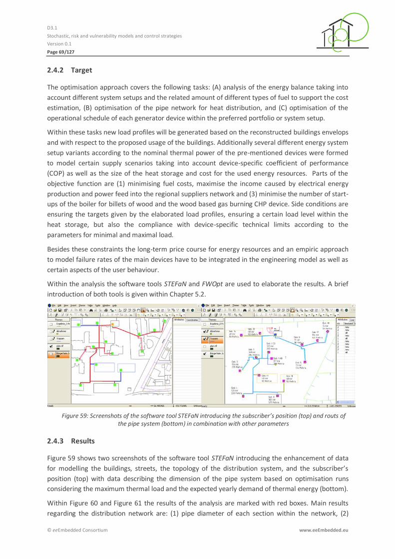
D3.1


Version 0.1

Page 69/127


Target 2.4.2

The optimisation approach covers the following tasks: (A) analysis of the energy balance taking into

account different system setups and the related amount of different types of fuel to support the cost

estimation, (B) optimisation of the pipe network for heat distribution, and (C) optimisation of the

operational schedule of each generator device within the preferred portfolio or system setup.

Within these tasks new load profiles will be generated based on the reconstructed buildings envelops

and with respect to the proposed usage of the buildings. Additionally several different energy system

setup variants according to the nominal thermal power of the pre-mentioned devices were formed

to model certain supply scenarios taking into account device-specific coefficient of performance

(COP) as well as the size of the heat storage and cost for the used energy resources. Parts of the

objective function are (1) minimising fuel costs, maximise the income caused by electrical energy

production and power feed into the regional suppliers network and (3) minimise the number of start-

ups of the boiler for billets of wood and the wood based gas burning CHP device. Side conditions are

ensuring the targets given by the elaborated load profiles, ensuring a certain load level within the

heat storage, but also the compliance with device-specific technical limits according to the

parameters for minimal and maximal load.

Besides these constraints the long-term price course for energy resources and an empiric approach

to model failure rates of the main devices have to be integrated in the engineering model as well as

certain aspects of the user behaviour.

Within the analysis the software tools STEFaN and FWOpt are used to elaborate the results. A brief

introduction of both tools is given within Chapter 5.2.

Figure 59: Screenshots of the software tool STEFaN introducing the subscriber’s position (top) and routs of the pipe system (bottom) in combination with other parameters

Results 2.4.3

Figure 59 shows two screenshots of the software tool STEFaN introducing the enhancement of data

for modelling the buildings, streets, the topology of the distribution system, and the subscriber’s

position (top) with data describing the dimension of the pipe system based on optimisation runs

considering the maximum thermal load and the expected yearly demand of thermal energy (bottom).

Within Figure 60 and Figure 61 the results of the analysis are marked with red boxes. Main results

regarding the distribution network are: (1) pipe diameter of each section within the network, (2)

D3.1


Version 0.1

Page 70/127


total length of the network, (3) normative mass flux for each section, (4) heat loss over the observed

analysis period, as well as (5) investment costs in total and for each section. Additional results are (6)

yearly operational costs and (7) the financial income due to power feed back into the regional

electricity distribution network.

In the sense of a Monte Carlo simulation (MCS) the standard thermal load profiles introduced within

Chapter 2.2.3 are processed 35 times taking into consideration a probability distribution of the

thermal load. As an example the resulting thermal load profiles within a typical week at the

beginning of the heating season are presented in Figure 62 as summarised heat demand for the

social care centre with a rough probabilistic approach for modelling the uncertainties according to

the user behaviour.

Each of the 35 realisations of a thermal load profile is applied to the four design variants covering a

different setup of heating generators and storage devices to calculate the energy demand as a basis

for the calculation of yearly operational costs. The resulting cost range for each variant is given in

Figure 63 as candlestick symbols.

Based on an individual estimation of mean time before failure (MTBF) and mean time to repair

(MTTR) for each individual heat generator type the up-time/down-time-schedule is processed for an

analysis period of one year to consider the reliability/dependability within the cost calculation. Figure

64 contains an overview of the availability for each individual heat generator type within one year

shown for each sample. Along the Y-axis the samples are applied. The down-time is expressed as

zero, availability-time is expressed as one. Within the graph on the top the values for the CHP-device

are displayed. Because of the youngish and more complex technology the down-time-periods are

more numerous and longer for CHP compared with the matured technology of the gas fired boiler,

described with the graph on the bottom. The woodchip boiler is situated in between both pre-

mentioned technologies from the reliability point of view.

With respect to the duration of the building lifecycle the analysis covers an estimation of the price for

the different sources of energy used within the variants. Figure 65 contains the results of the

probability density of prices for each energy source in year 2020 (left) and year 2030 (right),

estimated for woodchips (top), electricity (middle), as well as natural gas (bottom).

As shown in Figure 63 the variant with a CHP device delivering 30 kW electrical power in combination

with an heat storage of 750 kWh of thermal capacity and generates the lowest yearly cost lower than

200.000 Euro to average per year of about 200.000 Euro over all 35 processed samples while

considering the pre-described border conditions and constrains.

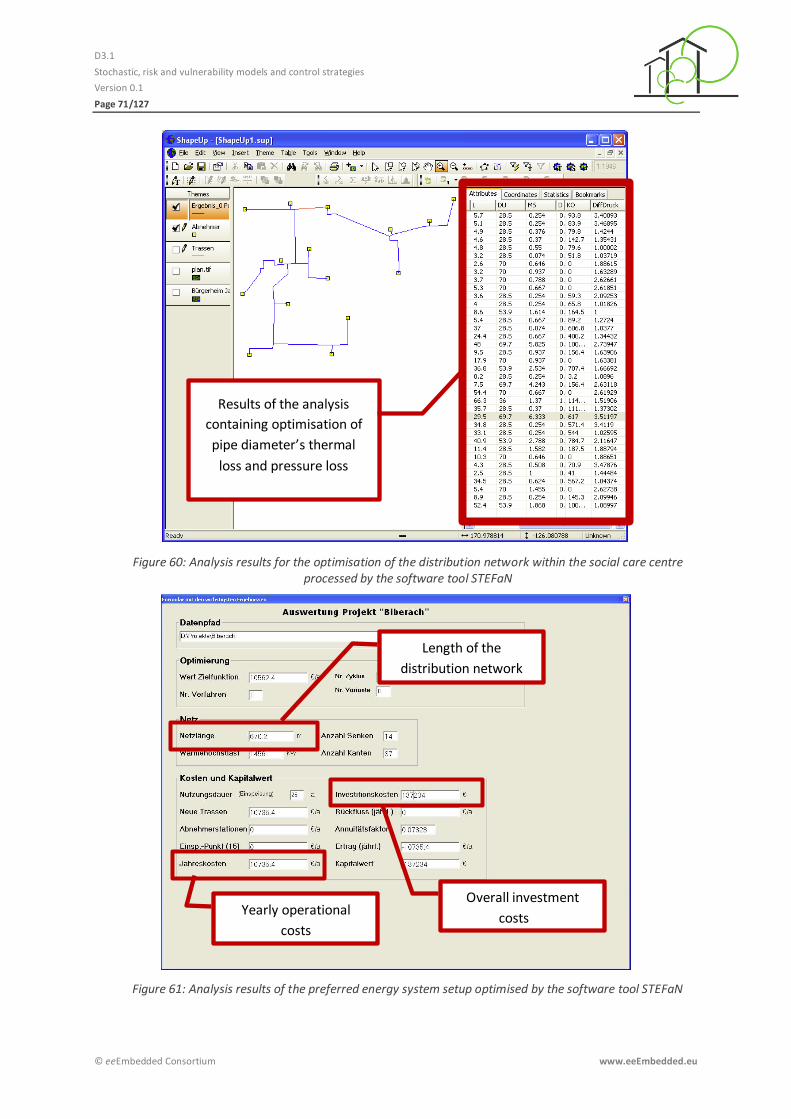
D3.1


Version 0.1

Page 71/127


Figure 60: Analysis results for the optimisation of the distribution network within the social care centre processed by the software tool STEFaN

Figure 61: Analysis results of the preferred energy system setup optimised by the software tool STEFaN

Length of the

distribution network

Overall investment

costs Yearly operational

costs

Results of the analysis

containing optimisation of

pipe diameter’s thermal

loss and pressure loss

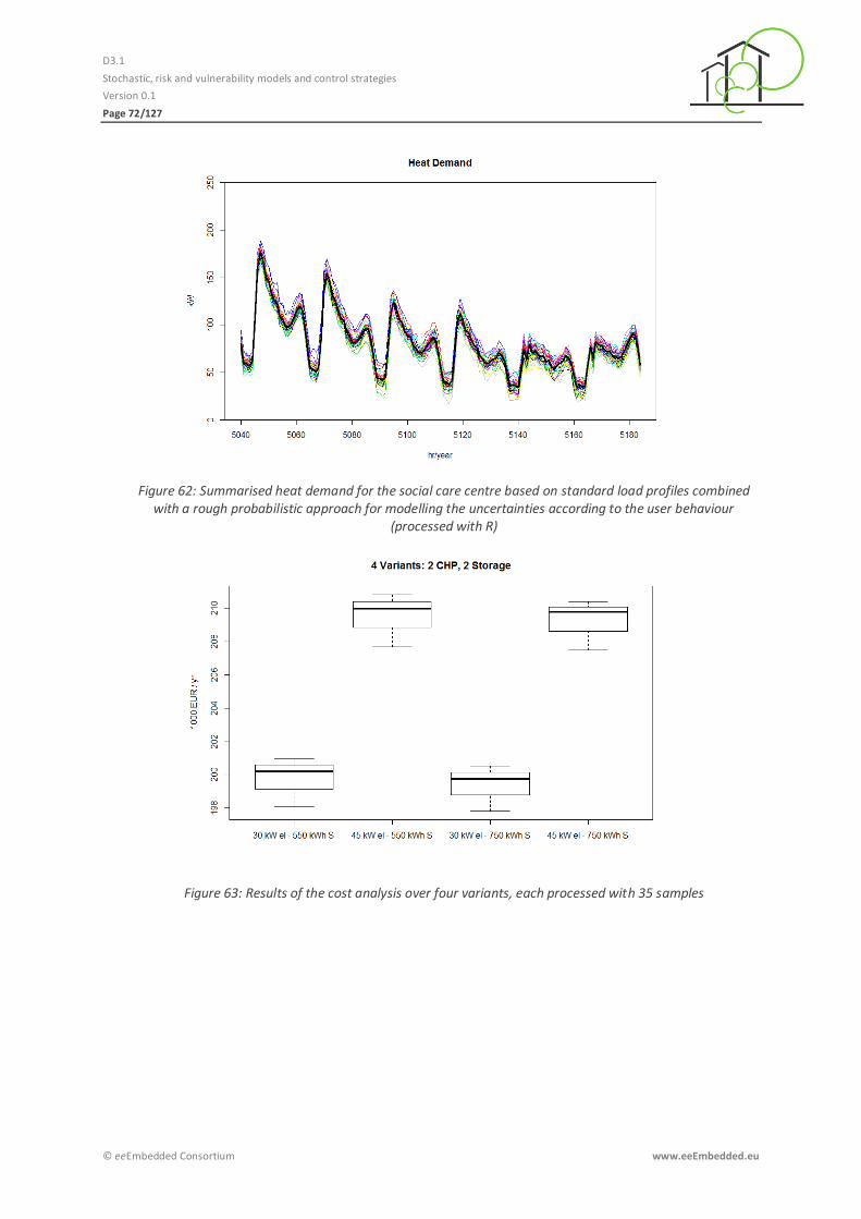
D3.1


Version 0.1

Page 72/127


Figure 62: Summarised heat demand for the social care centre based on standard load profiles combined with a rough probabilistic approach for modelling the uncertainties according to the user behaviour

(processed with R)

Figure 63: Results of the cost analysis over four variants, each processed with 35 samples

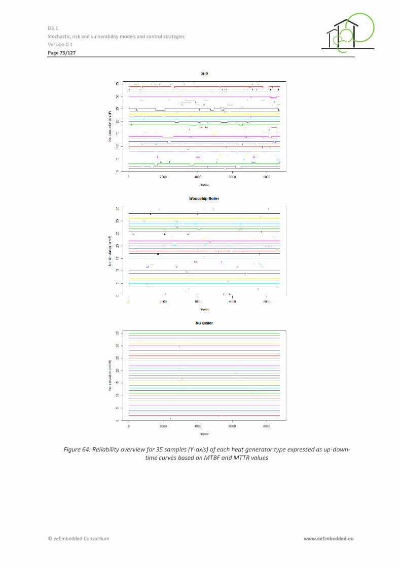
D3.1


Version 0.1

Page 73/127


Figure 64: Reliability overview for 35 samples (Y-axis) of each heat generator type expressed as up-down-time curves based on MTBF and MTTR values

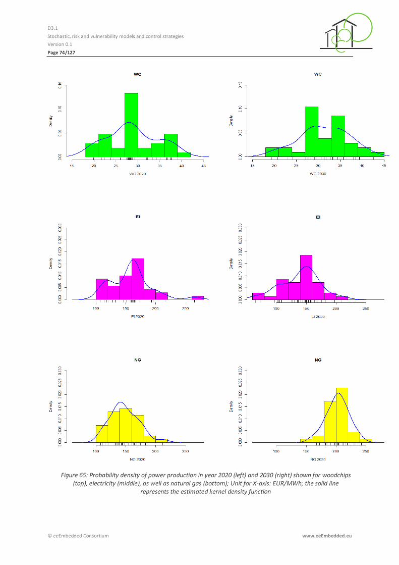
D3.1


Version 0.1

Page 74/127


Figure 65: Probability density of power production in year 2020 (left) and 2030 (right) shown for woodchips (top), electricity (middle), as well as natural gas (bottom); Unit for X-axis: EUR/MWh; the solid line

represents the estimated kernel density function

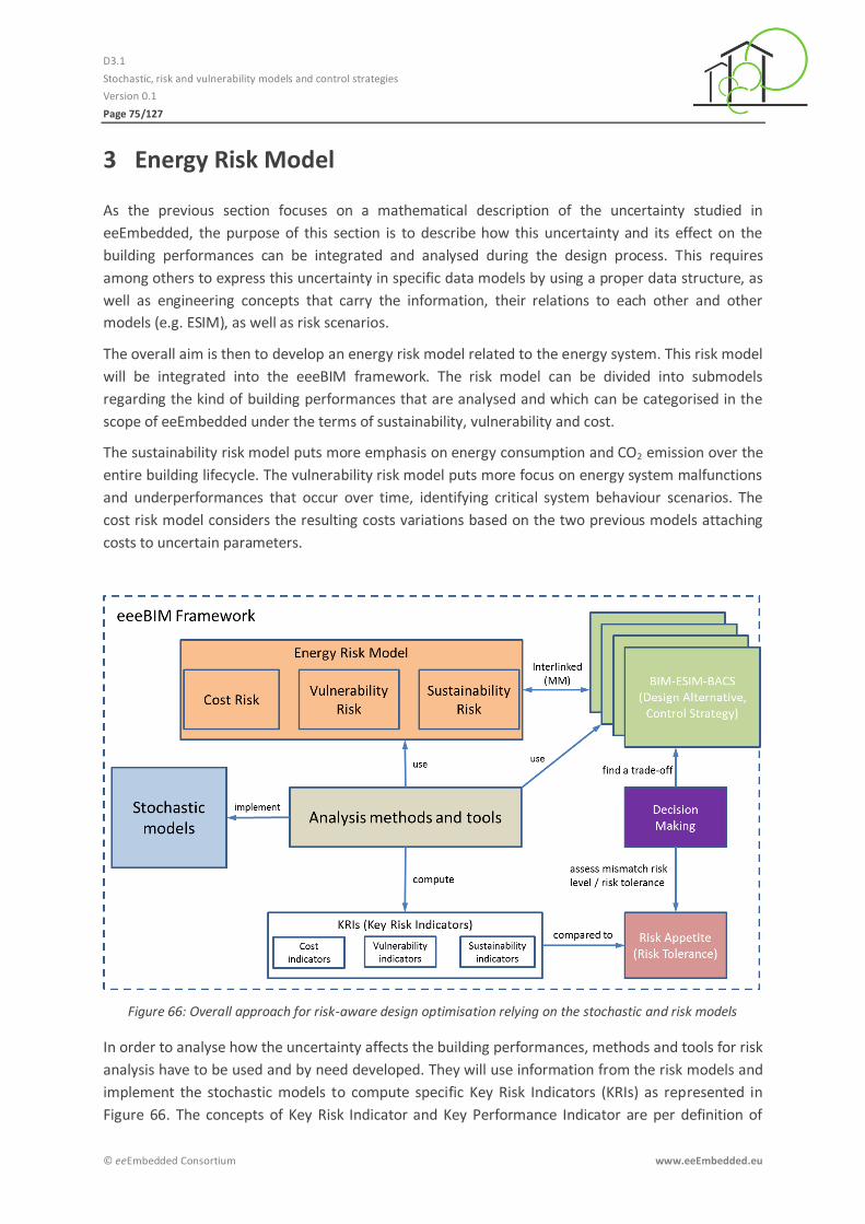
D3.1


Version 0.1

Page 75/127


3 Energy Risk Model

As the previous section focuses on a mathematical description of the uncertainty studied in

eeEmbedded, the purpose of this section is to describe how this uncertainty and its effect on the

building performances can be integrated and analysed during the design process. This requires

among others to express this uncertainty in specific data models by using a proper data structure, as

well as engineering concepts that carry the information, their relations to each other and other

models (e.g. ESIM), as well as risk scenarios.

The overall aim is then to develop an energy risk model related to the energy system. This risk model

will be integrated into the eeeBIM framework. The risk model can be divided into submodels

regarding the kind of building performances that are analysed and which can be categorised in the

scope of eeEmbedded under the terms of sustainability, vulnerability and cost.

The sustainability risk model puts more emphasis on energy consumption and CO2 emission over the

entire building lifecycle. The vulnerability risk model puts more focus on energy system malfunctions

and underperformances that occur over time, identifying critical system behaviour scenarios. The

cost risk model considers the resulting costs variations based on the two previous models attaching

costs to uncertain parameters.

Figure 66: Overall approach for risk-aware design optimisation relying on the stochastic and risk models

In order to analyse how the uncertainty affects the building performances, methods and tools for risk

analysis have to be used and by need developed. They will use information from the risk models and

implement the stochastic models to compute specific Key Risk Indicators (KRIs) as represented in

Figure 66. The concepts of Key Risk Indicator and Key Performance Indicator are per definition of

D3.1


Version 0.1

Page 76/127


similar nature but serve distinct purposes. In a common understanding the concept of KRI is often

defined as the inverse concept of KPI which is not always the case. Both should be either minimised

or maximised according to the kind of performance of interest and the design goals. For example

when minimising the energy demand (KPI) a designer wishes to minimise the uncertainty on the

energy demand value (KRI) as well. Another simple example of KRI is the failure frequency of an

energy subsystem which can be modelled as a failure frequency function in a stochastic model. This

function uses the hazard rates of the components of the energy subsystem. The description of

component interactions and their hazard rate properties are then part of the vulnerability risk model.

The analysis tool would calculate the failure frequency which can be expressed as KRI. Based on this

KRI design alternatives and facility management guidelines can be derived, expressed as control

strategies or maintenance plans, that would reduce the KRI value to an acceptable level.

3.1 Sustainability, Vulnerability and Cost Risk Models

Requirements for a Sustainability Risk Model 3.1.1

Per definition sustainability concentrates on maintaining performances over the entire life cycle of a

building. However the meaning of this word has been extended with the appearance of the Green

Building concept or Sustainable Building and the related environmental guidelines (LEED, 2011). In

the scope of the project this issue concentrates mostly on energy consumption and CO2 emission

that have to be kept in reasonable and targeted quantities over decades. The assessment of energy

use and CO2 emission will rely on the model developed in Task 3.1. The purpose of the sustainability

risk model is first to catch relevant information for this stochastic model by referencing factors of

influence from the related stochastic models. These are primary the technological progress,

influencing the energy efficiency of building elements, as well as the climate and the building usage,

both directly influencing the building’s energy consumption and CO2 emission. Second the

sustainability risk model has to draw up scenarios of cyclic peak loads and resulting changes in the

overall energy balance leading to more exhaust gas and wasted energy. For CO2 emission the

characteristics of the energy system are also of importance and especially the kind of energy used. It

is essential to differentiate between high carbon power technologies using fossil energy sources like

fuel or gas boilers and low carbon power technologies like wind power, solar power, geothermal

power, etc. At a lower level of granularity, the components of such technologies also have specific

energy and CO2 related characteristics. Sustainability indices can then be allocated to those different

technologies and components, thus enabling the planner to get an idea of the actual sustainability

risk of the design choices he makes. Examples for these indices are heating, cooling or energy

demand or the number of hours, a certain temperature threshold is exceeded.

Requirements for a Vulnerability Risk Model 3.1.2

To model the system vulnerability it is necessary to identify all parameters that influence the system

behaviour. In this sense the components characteristics are of importance as well as their

interactions. Such information like component lifetime, hazard rates and the composition of

components has to be described in the model. Fault trees are used to model the hierarchic

propagation of faults from component to system level. External factors are also of importance like

the energy demand resulting for example from the building usage and the climate. Moreover,

D3.1


Version 0.1

Page 77/127


vulnerability does not only mean failure but also underperformance. The level of redundancy, as well

as the frequency and intensity of energy peak loads play an essential role in maintaining the system

performance. Having redundant components like building energy sources at building level (boilers,

PV, solar thermal panels, etc.) and at district level (power plants, wind turbines, neighbour buildings,

etc.) is somehow necessary to ensure covering the building energy demand even when components

fail or peak loads occur. More than only to cover energy demand, it is also of importance that the

system components work at their efficient load by avoiding overload of some devices which

enhances wear and reduces yield. In the same sense, the system should avoid under-speed of

devices to reduce yield. Together with the characterisation of the system properties and the external

factors, it is also important to identify risk cases or scenarios describing critical behaviours on the

basis of components’ interactions. Those risk scenarios are also part of the vulnerability risk model.

Typical values that are extracted from the vulnerability risk model are system overspeed and

underspeed, failure rate, mean time to failure or repair and availability data such as point availability

or interval availability.

To summarise, the following main aspects can be considered under the concept of vulnerability:

- Underperformance e.g. wrong energy balance between supply, use, storage, transmission and distribution, or bad devices yield

- Failure e.g. breakdowns, damages, blackouts - Malfunction e.g. wrong sensor values, wrong devices setup

Requirements for a Cost Risk Model 3.1.3

The cost risk model references all items that have an influence on the overall costs of the building.

The main drivers here are energy prices and technological progress. During the whole building

lifecycle those costs occur in the different phases of the project from design/retrofit over

construction to exploitation. Focusing on energy and the energy system the costs can be classified in

the three following categories:

Energy system costs: HVAC, BACS devices unit costs and installation costs.

Operation costs: energy price with fix and variable parts depending on the energy market

Maintenance costs: spare parts unit costs, labour costs, consumable resource costs (from vulnerability risk model)

The risk model has to describe the uncertainty over costs by using suitable representations that

express their random character. Here the probability distributions of cost-related KPIs like

construction cost, energy system cost or maintenance cost are appropriate.

3.2 Key Risk Indicator Framework

The activity of analysing and controlling risk has been of growing interest since the last decade and is

increasingly establishing itself as a necessary and systematic management procedure in different

industries. Especially, since the publication of the international standard (ISO/IEC 31000:2009) about

risk management this trend has accelerated. This standard has resulted from an assembly of several

previous standards and guidelines developed in the last two decades in different countries. This has

made it an internationally recognised reference for risk management. The standard applies to any

organisation regardless of its size, activity or sector. In parallel to the development of the standards

D3.1


Version 0.1

Page 78/127


relative young domains applying them and feeding them with new findings have emerged like among

others Operational Risk Management (ORM), Enterprise Risk Management (ERM) and Project Risk

Management (PRM). The main application area of such domains is and has always been the

corporate and market finance field which is the precursor for the development of risk management

techniques. Nevertheless, as mentioned above such techniques and related concepts spread

themselves to the industries of manufacturing and services in general, and especially in activities

commonly associated with high risk levels like in chemical and medical industries. In the AEC industry

there is still a poor use of risk management techniques. Some current risk management methods

that are currently applied examine risk as a rather isolated purpose in the context of traditional

management techniques that break down the project into manageable, self-contained subtasks

within specific application fields like project scheduling and cost planning. Also, risk management is

still done mostly occasionally during a project as it should be accomplished continuously throughout

all project phases and began already in a very early project state. In order to bridge these gaps, it

become of interest to take benefit of the latest risk management techniques applied in other fields

and to integrate them into the innovative research activities made in the context of eeEmbedded

and in the BIM community in general.

Application of risk management concepts 3.2.1

As stated by (Beasley et al., 2011) ERM provides the opportunity for organisational leaders to achieve

a robust and holistic enterprise-wide view of potential risks that may affect the achievement of the

organisation’s objectives. As for corporate management a building project is an organised and

collaborative activity that aims at the achievement of a final product with regard to precise

requirements expressed by clients and decision makers. In view of that it also requires to get a good

overview of risk in order to support design and investment decisions that minimise the probability of

performance mismatches. In order to enable a holistic view and efficient control of risk, techniques

and concepts from the risk management domains like KRIs (Key Risk Indicators) are brought into the

eeEmbedded project.

As represented on Figure 67 the ISO standard (ISO/IEC 31000:2009) defines four essential steps that

have to be executed in a dynamic way as parts of a risk management cycle comprising risk

identification, risk analysis, risk treatment and risk monitoring. Risk identification performs an

exhaustive listing of all possible threats, their categorisation, and the recognition of the affected

models instances as well as of risk chains. Risk analysis enables the evaluation and prioritisation of

risks with help of risk simulations. Risk treatment planning consists of determining preventive

measures and reaction strategies to reduce threats to the project objectives and to enhance

reactivity. Within the execution phase of the project the risk monitoring and control tasks

continuously re-evaluate the suitability of the planned treatment measures and support identifying

new emerging risks. In a similar way, as mentioned by (Sherwood, 2012) ERM defines the five

following steps for performing risk management: 1. identify risks, 2. describe and/or quantify risks, 3.

decide how to mitigate risks, 4. implement decisions, 5. monitor results of decisions and make

changes as needed.

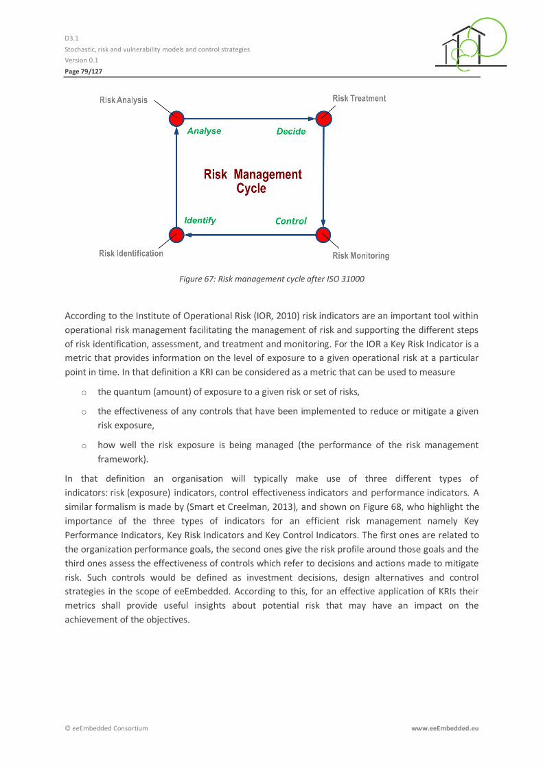
D3.1


Version 0.1

Page 79/127


Figure 67: Risk management cycle after ISO 31000

According to the Institute of Operational Risk (IOR, 2010) risk indicators are an important tool within

operational risk management facilitating the management of risk and supporting the different steps

of risk identification, assessment, and treatment and monitoring. For the IOR a Key Risk Indicator is a

metric that provides information on the level of exposure to a given operational risk at a particular

point in time. In that definition a KRI can be considered as a metric that can be used to measure

o the quantum (amount) of exposure to a given risk or set of risks,

o the effectiveness of any controls that have been implemented to reduce or mitigate a given

risk exposure,

o how well the risk exposure is being managed (the performance of the risk management

framework).

In that definition an organisation will typically make use of three different types of

indicators: risk (exposure) indicators, control effectiveness indicators and performance indicators. A

similar formalism is made by (Smart et Creelman, 2013), and shown on Figure 68, who highlight the

importance of the three types of indicators for an efficient risk management namely Key

Performance Indicators, Key Risk Indicators and Key Control Indicators. The first ones are related to

the organization performance goals, the second ones give the risk profile around those goals and the

third ones assess the effectiveness of controls which refer to decisions and actions made to mitigate

risk. Such controls would be defined as investment decisions, design alternatives and control

strategies in the scope of eeEmbedded. According to this, for an effective application of KRIs their

metrics shall provide useful insights about potential risk that may have an impact on the

achievement of the objectives.

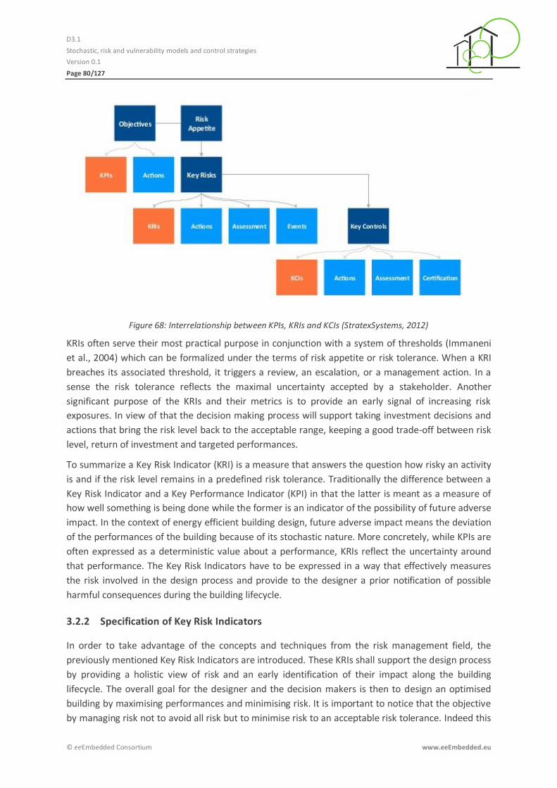
D3.1


Version 0.1

Page 80/127


Figure 68: Interrelationship between KPIs, KRIs and KCIs (StratexSystems, 2012)

KRIs often serve their most practical purpose in conjunction with a system of thresholds (Immaneni

et al., 2004) which can be formalized under the terms of risk appetite or risk tolerance. When a KRI

breaches its associated threshold, it triggers a review, an escalation, or a management action. In a

sense the risk tolerance reflects the maximal uncertainty accepted by a stakeholder. Another

significant purpose of the KRIs and their metrics is to provide an early signal of increasing risk

exposures. In view of that the decision making process will support taking investment decisions and

actions that bring the risk level back to the acceptable range, keeping a good trade-off between risk

level, return of investment and targeted performances.

To summarize a Key Risk Indicator (KRI) is a measure that answers the question how risky an activity

is and if the risk level remains in a predefined risk tolerance. Traditionally the difference between a

Key Risk Indicator and a Key Performance Indicator (KPI) in that the latter is meant as a measure of

how well something is being done while the former is an indicator of the possibility of future adverse

impact. In the context of energy efficient building design, future adverse impact means the deviation

of the performances of the building because of its stochastic nature. More concretely, while KPIs are

often expressed as a deterministic value about a performance, KRIs reflect the uncertainty around

that performance. The Key Risk Indicators have to be expressed in a way that effectively measures

the risk involved in the design process and provide to the designer a prior notification of possible

harmful consequences during the building lifecycle.

Specification of Key Risk Indicators 3.2.2

In order to take advantage of the concepts and techniques from the risk management field, the

previously mentioned Key Risk Indicators are introduced. These KRIs shall support the design process

by providing a holistic view of risk and an early identification of their impact along the building

lifecycle. The overall goal for the designer and the decision makers is then to design an optimised

building by maximising performances and minimising risk. It is important to notice that the objective

by managing risk not to avoid all risk but to minimise risk to an acceptable risk tolerance. Indeed this

D3.1


Version 0.1

Page 81/127


error is often made in the praxis because reducing risk implies taking investment decisions and

actions that consume resource and generate costs, thus impacting the performances. That is why the

concepts of KRIs and risk tolerance are both introduced and play a complementary role to the KPIs.

The KCIs are not integrated in the overall risk management approach described in this deliverable,

but could be developed in future works in the context of the operation phase of the building

lifecycle.

As for the submodels of the Energy Risk Model the Key Risk Indicators can be classified in the three

main categories of sustainability, vulnerability and cost. Specifying KRIs in those three categories and

selecting some of them for the implementation of a prototype would provide an already wide and

interdisciplinary view of risk as support for a proof of concept.

In the context of eeEmbedded the Key Risk Indicators can either provide a measure of uncertainty

around certain KPIs or they can specifically express certain underperformances and critical states

that do not relate to predefined KPIs. In the context of sustainability and cost it is of interest to

evaluate the deviations in KPI values caused by uncertainty. This can be done for energy

consumption, gas emission and costs on the basis of the eeE KPIs specified in (Guruz et al., 2014). In

view of that this performance deviation represents the risk to which a KRI relates, except for the

thermal comfort. A KRI can then be defined on the basis of the value distribution of a KPI resulting

from uncertainty. In other words it can be defined as a statistical indicator deduced from the

probability distribution of a KPI. For that purpose indicators like standard deviation (σ), mean and

mode (most probable value) are used. Other interesting indicators would also be the probability of

being over or beneath the KPI target value or even being in or outside a certain value range. Such

indicators are also easily deduced from the probability distribution of a KPI. For vulnerability and

thermal comfort (sustainability) other kinds of indicators have to be introduced that express how

building performance can be threatened by risk and that are independent from the predefined eeE

KPIs. Most of them are also defined in terms of probabilistic values. In view of that a set of KRIs for

eeEmbedded has been specified and they are listed in Table 12, Table 13 and Table 14. In each table

the KRI category, a subcategory, a KRI type, KRIs and a unit are defined. The latter two define the KRI

metrics.

Table 12: KRIs in sustainability category

Category Subcategory Key Risk Indicator type KRIs Unit

Sustainability

Energy

consumption

Uncertainty on heating demand σ , mode, mean kWh/(m².a)

Uncertainty on cooling demand σ , mode, mean kWh/(m².a)

Uncertainty on electrical energy demand σ , mode, mean kWh/(m².a)

Uncertainty on primary energy use σ , mode, mean kWh/(m².a)

Uncertainty on total energy demand σ , mode, mean kWh/(m².a)

CO2 Emission Uncertainty on CO2 emission σ , mode, mean Kg/(m².a)

Thermal

comfort

Pre-heating time σ , mode, mean Kh

Pre-cooling time σ , mode, mean Kh

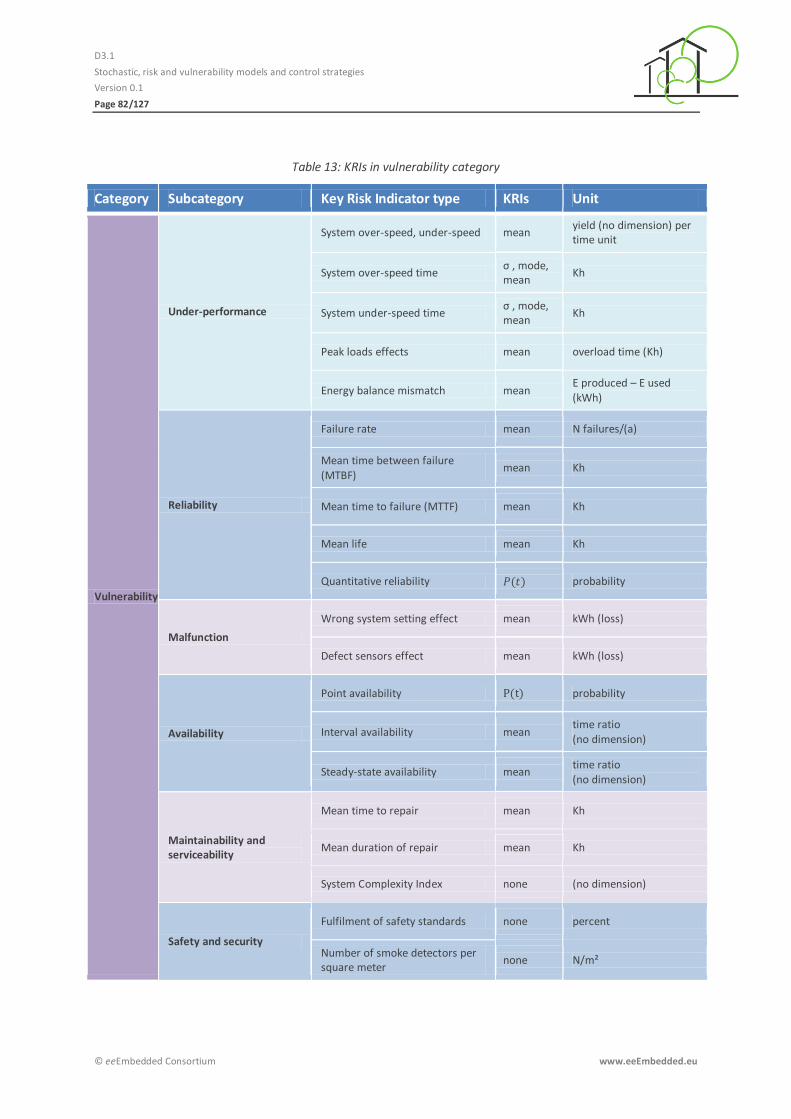
D3.1


Version 0.1

Page 82/127


Table 13: KRIs in vulnerability category


Vulnerability

Under-performance

System over-speed, under-speed mean yield (no dimension) per time unit

System over-speed time σ , mode, mean

Kh

System under-speed time σ , mode, mean

Kh

Peak loads effects mean overload time (Kh)

Energy balance mismatch mean E produced – E used (kWh)

Reliability

Failure rate mean N failures/(a)

Mean time between failure (MTBF)

mean Kh

Mean time to failure (MTTF) mean Kh

Mean life mean Kh

Quantitative reliability probability

Malfunction

Wrong system setting effect mean kWh (loss)

Defect sensors effect mean kWh (loss)

Availability

Point availability probability

Interval availability mean time ratio (no dimension)

Steady-state availability mean time ratio (no dimension)

Maintainability and serviceability

Mean time to repair mean Kh

Mean duration of repair mean Kh

System Complexity Index none (no dimension)

Safety and security

Fulfilment of safety standards none percent

Number of smoke detectors per square meter

none N/m²

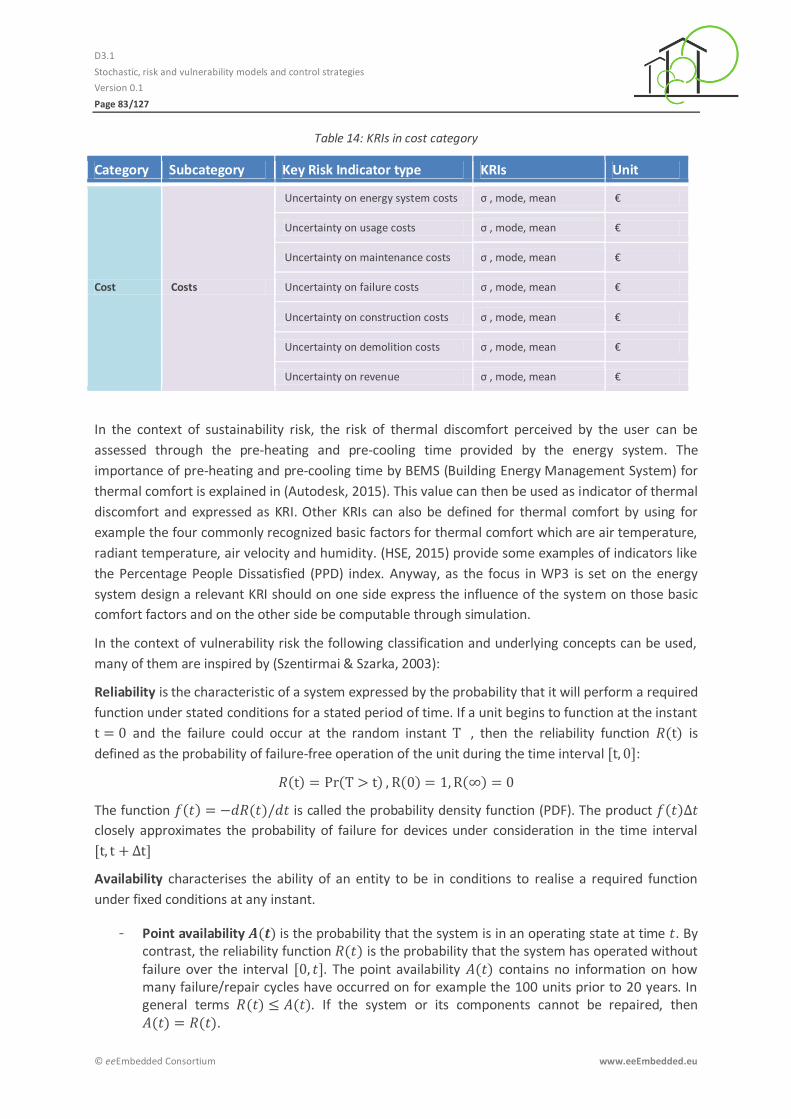
D3.1


Version 0.1

Page 83/127


Table 14: KRIs in cost category


Cost Costs

Uncertainty on energy system costs σ , mode, mean €

Uncertainty on usage costs σ , mode, mean €

Uncertainty on maintenance costs σ , mode, mean €

Uncertainty on failure costs σ , mode, mean €

Uncertainty on construction costs σ , mode, mean €

Uncertainty on demolition costs σ , mode, mean €

Uncertainty on revenue σ , mode, mean €

In the context of sustainability risk, the risk of thermal discomfort perceived by the user can be

assessed through the pre-heating and pre-cooling time provided by the energy system. The

importance of pre-heating and pre-cooling time by BEMS (Building Energy Management System) for

thermal comfort is explained in (Autodesk, 2015). This value can then be used as indicator of thermal

discomfort and expressed as KRI. Other KRIs can also be defined for thermal comfort by using for

example the four commonly recognized basic factors for thermal comfort which are air temperature,

radiant temperature, air velocity and humidity. (HSE, 2015) provide some examples of indicators like

the Percentage People Dissatisfied (PPD) index. Anyway, as the focus in WP3 is set on the energy

system design a relevant KRI should on one side express the influence of the system on those basic

comfort factors and on the other side be computable through simulation.

In the context of vulnerability risk the following classification and underlying concepts can be used,

many of them are inspired by (Szentirmai & Szarka, 2003):

Reliability is the characteristic of a system expressed by the probability that it will perform a required

function under stated conditions for a stated period of time. If a unit begins to function at the instant

and the failure could occur at the random instant , then the reliability function is

defined as the probability of failure-free operation of the unit during the time interval :

The function is called the probability density function (PDF). The product

closely approximates the probability of failure for devices under consideration in the time interval

Availability characterises the ability of an entity to be in conditions to realise a required function

under fixed conditions at any instant.

- Point availability is the probability that the system is in an operating state at time . By contrast, the reliability function is the probability that the system has operated without failure over the interval . The point availability contains no information on how many failure/repair cycles have occurred on for example the 100 units prior to 20 years. In general terms . If the system or its components cannot be repaired, then .

D3.1


Version 0.1

Page 84/127


- Interval (mission) availability is the expected fractional amount of an interval of specified length that the system is in an operable state. This interval may be the design life of the system or the time to accomplish some particular mission.

- Steady-state (asymptotic, limiting) availability is the limit of interval availability for an infinite interval. If the system under consideration is not repairable, then its steady-state availability is equal to zero.

Maintainability and serviceability characterise the ability of an entity to be maintained or restored

to a state in which it can realise a required function when maintenance is done under fixed

conditions with prescribed procedures and means. Hereby, serviceability describes the features that

facilitate and speed-up maintenance actions. An important aspect for the maintainability of a system

is its complexity. It is possible to quantify it with a system complexity index, as demonstrated in

(Wohl, 1982) which we can also use as indicator for maintainability risk.

Safety and security characterise the ability of an entity to meet fixed conditions and to avoid critical

or catastrophic events. Hereby safety protects against accidents while security protects against

intentional induced harms like sabotage.

Underperformance characterises a state in which the system cannot develop its full potential

performance. Reasons may be a wrong energy balance between supply, use, storage, transmission

and distribution or a suboptimal yield. It is to notice that underperformance can be among others the

result of a lack of reliability or availability.

Malfunction describes a state in which a component or a subsystem do not perform its expected

function because for example of a defect sensors delivering wrong values or bad device

configuration.

3.3 Risk analysis workflow for optimised building design under uncertainty

In the following chapter, a detailed risk analysis workflow for the consideration of uncertainty in the

building design process is developed. This workflow is meant to be integrated in the eeE Key Point

Framework, established in Deliverable 2.1 (Guruz et al., 2014). The focus of this framework is to

enable a KPI-driven design optimisation, meaning that an optimal design can be assessed through

several KPIs that have to fulfill target values. For the risk analysis workflow the major tools we

dispose of are Alternative Analysis (AA), comparing different design solutions and their KPIs,

Sensitivity Analysis (SA), deriving the impact of design variables on the KPIs and Uncertainty Analysis

(UA) yielding the probability distributions of the KPIs and thus deriving the KRIs (see Chapter 3.1).

At first a short overview over different SA methods and their features is given (see Chapter 3.3.1).

Then the general work flow is established (see Chapter 3.3.2). Finally the exact methods for every

step of the workflow are chosen and explained (see Chapter 3.3.3).

Sensitivity Analysis overview 3.3.1

There are several kinds of SA methods available which for our purposes will be distinguished in three

groups: Local SA, global SA and screening.

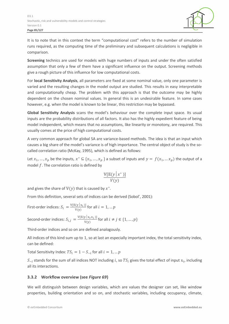
D3.1


Version 0.1

Page 85/127


It is to note that in this context the term “computational cost” refers to the number of simulation

runs required, as the computing time of the preliminary and subsequent calculations is negligible in

comparison.

Screening technics are used for models with huge numbers of inputs and under the often satisfied

assumption that only a few of them have a significant influence on the output. Screening methods

give a rough picture of this influence for low computational costs.

For local Sensitivity Analysis, all parameters are fixed at some nominal value, only one parameter is

varied and the resulting changes in the model output are studied. This results in easy interpretable

and computationally cheap. The problem with this approach is that the outcome may be highly

dependent on the chosen nominal values. In general this is an undesirable feature. In some cases

however, e.g. when the model is known to be linear, this restriction may be bypassed.

Global Sensitivity Analysis scans the model’s behaviour over the complete input space. Its usual

inputs are the probability distributions of all factors. It also has the highly expedient feature of being

model independent, which means that no assumptions, like linearity or monotony, are required. This

usually comes at the price of high computational costs.

A very common approach for global SA are variance-based methods. The idea is that an input which

causes a big share of the model’s variance is of high importance. The central object of study is the so-

called correlation ratio (McKay, 1995), which is defined as follows:

Let be the inputs, a subset of inputs and the output of a

model . The correlation ratio is defined by

and gives the share of that is caused by .

From this definition, several sets of indices can be derived (Sobol’, 2001):

First-order indices:

for all

Second-order indices:

for all

Third-order indices and so on are defined analogously.

All indices of this kind sum up to , so at last an especially important index, the total sensitivity index,

can be defined:

Total Sensitivity Index: for all

stands for the sum of all indices NOT including , so gives the total effect of input , including

all its interactions.

Workflow overview (see Figure 69) 3.3.2

We will distinguish between design variables, which are values the designer can set, like window

properties, building orientation and so on, and stochastic variables, including occupancy, climate,

D3.1


Version 0.1

Page 86/127


technological progress and energy prices (see Chapter 2.2.4). Reliability is modelled separately and

will not be part of the sensitivity analysis.

In the eeEmbedded approach (Guruz et al., 2014), at first several KPIs of interest are chosen and

target ranges, meaning values regarded as desirable, are assigned. These are also known as KPIs to-

be.

For a more holistic impression it may be beneficial to form new KPIs, combining existing ones. One

way to do so is by creating a composition of KPIs, possibly including weighting, e.g.

. When using this approach, some kind of standardisation has to be

applied, e.g. transforming all KPIs to , to counteract the impact of different units of

measurement and orders of magnitude. Also, if negative values are possible, it is advisable to use the

absolute values of the KPIs.

Another way is to set thresholds for existing KPIs, e.g. {

.

It is to note that for such a KPI, the following distinction between a linear and a non-linear impact of

an input may be meaningless (see Chapter 3.3.3).

Than the KRIs to-be, which express the risk tolerance mentioned in Chapter 3.2 are chosen, meaning

some KRIs of interest are picked and target ranges are assigned.

The next step is to compare the performance of some manually chosen design alternatives by

performing an AA. After the most appealing one is picked for profound examination, one has to

decide which design variables should be varied and which should be fixed in the subsequent

analyses, e.g. because they are default values that are not changeable, or because they are of no

interest.

Next is the execution of a screening to distinguish between three categories of inputs: (a) negligible,

(b) linear and additive or (c) non-linear or involved in interactions with other factors.

The non-important factors can be fixed at a nominal value, e.g. at their expected value and are of no

further interest.

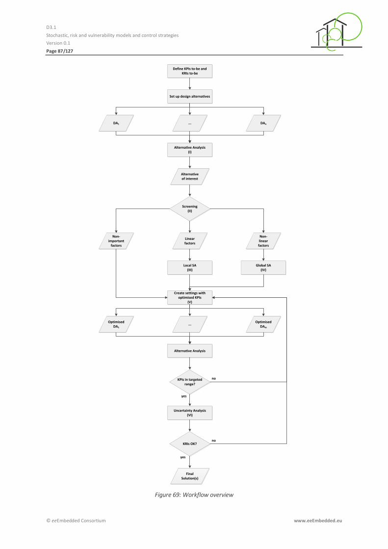
D3.1


Version 0.1

Page 87/127


Define KPIs to-be andKRIs to-be

Alternative Analysis(I)

Create settings with optimised KPIs

(V)

Local SA(III)

Set up design alternatives

...DA1 DAn

Alternative of interest

Screening(II)

Linear factors

Non-important

factors

Non-linear

factors

Global SA(IV)

...Optimised

DA1

Optimised DAm

Alternative Analysis

KPIs in targeted range?

Uncertainty Analysis(VI)

KRIs OK?

Final Solution(s)

yes

yes

no

no

Figure 69: Workflow overview

D3.1


Version 0.1

Page 88/127


For the linear inputs a local SA is performed, because for them, the arbitrary chosen values of the

other inputs have no impact. For each KPI, this yields the strength and direction of the analysed

input.

For the non-linear factors, a global SA is performed to understand in detail which inputs interact with

each other and how strong their contribution is.

This procedure yields solid knowledge to create several design alternatives which aim at optimising

the targeted KPIs. To check the robustness of these settings an UA will be performed by repeatedly

sampling the involved stochastic variables. The result is the KPI’s probability distributions which can

be evaluated to verify the KRIs of interest.

Detailed Approach 3.3.3

To perform the initial AA (see Figure 69(I)), several design alternatives are created by assigning values

to all design variables. Then cases for the stochastic variables are chosen, like extremely cold climate,

high occupancy or the average cases. These cases are either predefined, like the data of an extremely

cold year, or are generated by repeated sampling and selecting an appropriate case, e.g. the energy

price development which constitutes the average of the drawn samples. Then the simulation is

executed with the same set of realisations of the stochastic variables for each design alternative. This

assures comparability. If reliability-based KPIs are of interest, for each design alternative several runs

of the reliability simulation (see Chapter 2.3.1.3) are performed to derive these KPIs. The resulting

KPIs are studied and a design alternative, meaning a setting of design variables is picked to be

explored deeper.

The screening method used in our approach (see Figure 69 (II)) will be the Morris One-At-a-Time

Design (Morris, 1991), which is the most widely used screening method. Its strength is, that it is

computational cheap, easy to calculate and interpret, but nevertheless quite precise. Its weakness is

that no distributions are considered. To further improve the method, two extensions proposed by

(Campolongo et al., 2007) are applied.

The main idea of the Morris method is the computation of several so called elementary effects (EEs)

for each input by varying one input at a time over a certain amount of fixed levels. For the design

variables, values according to the number of levels are picked from their range. The choice of these

values can be guided by the probability distribution of the factors or the length of their definition

range. Here it is advisable to use the lowest-level properties possible, e.g. to vary the U-value instead

of varying between several complete windows. This approach gives insights that will later on help to

decide for the most suitable solutions.

For the stochastic variables a case for every level has to be specified. A way to do this is to sample

the stochastic variable repeatedly and to select the cases sorted by a signature value, like e.g.

occupants density for occupancy. Then the method creates a sample plan, which tells what levels of

inputs are to be combined for simulations. An improved way to create this plan is the space fill

improvement of (Campolongo et al., 2007), which optimises the scanning of the input space. This

method considers possible EEs per factor and chooses the best ones to compute. This does not

increase the number of model evaluations required.

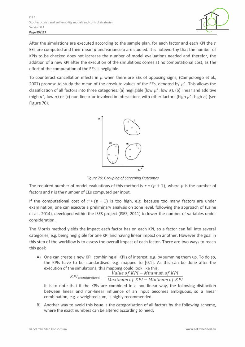
D3.1


Version 0.1

Page 89/127


After the simulations are executed according to the sample plan, for each factor and each KPI the

EEs are computed and their mean and variance σ are studied. It is noteworthy that the number of

KPIs to be checked does not increase the number of model evaluations needed and therefor, the

addition of a new KPI after the execution of the simulations comes at no computational cost, as the

effort of the computation of the EEs is negligible.

To counteract cancellation effects in when there are EEs of opposing signs, (Campolongo et al.,

2007) propose to study the mean of the absolute values of the EEs, denoted by . This allows the

classification of all factors into three categories: (a) negligible (low , low ), (b) linear and additive

(high , low ) or (c) non-linear or involved in interactions with other factors (high , high ) (see

Figure 70).

Figure 70: Grouping of Screening Outcomes

The required number of model evaluations of this method is , where is the number of

factors and is the number of EEs computed per input.

If the computational cost of is too high, e.g. because too many factors are under

examination, one can execute a preliminary analysis on zone level, following the approach of (Laine

et al., 2014), developed within the ISES project (ISES, 2011) to lower the number of variables under

consideration.

The Morris method yields the impact each factor has on each KPI, so a factor can fall into several

categories, e.g. being negligible for one KPI and having linear impact on another. However the goal in

this step of the workflow is to assess the overall impact of each factor. There are two ways to reach

this goal:

A) One can create a new KPI, combining all KPIs of interest, e.g. by summing them up. To do so, the KPIs have to be standardised, e.g. mapped to . As this can be done after the execution of the simulations, this mapping could look like this:

It is to note that if the KPIs are combined in a non-linear way, the following distinction between linear and non-linear influence of an input becomes ambiguous, so a linear combination, e.g. a weighted sum, is highly recommended.

B) Another way to avoid this issue is the categorisation of all factors by the following scheme, where the exact numbers can be altered according to need:

D3.1


Version 0.1

Page 90/127


I. If a KPI has a non-linear influence at least 10 % of the KPIs, it is considered non-linear.

II. If a KPI is not non-linear and has a linear influence at least 10 % of the KPIs, it is considered linear.

III. The remaining KPIs are considered negligible. Now the further treatment of the three groups is explained.

Treatment of group (a): As the impact of these inputs on the KPIs of interest is negligible, they can be

fixed at an arbitrary value in their range, e.g. the expected value or the midpoint of their range can

be chosen.

Treatment of group (b): Here, by calculating the difference quotient for each input, the simplest form

of local SA can be applied (see Figure 69 (III)). As it is known that the factor’s impact is linear, two

model evaluations are sufficient to determine the slope of the KPIs. As the factor is known to not

interact with other factors, these can be fixed at arbitrary values and for the stochastic variables, a

random sample or an arbitrary case, advisably not too extreme, can be used. The result is a number

for each KPI, giving the strength and the direction of the impact the factor has on this KPI.

Treatment of group (c): Here a more educated approach has to be applied. Depending on the set of

sensitivity indices (see Global SA in Chapter 3.3.1) one wants to derive, there are two advisable

global SA methods (see Figure 69 (IV)). If the aim is to discover the precise structure of interactions

between the inputs, the Sobol’ method (Sobol’, 2001) is appropriate. This method allows the

calculation of all sensitivity indices up to a certain order at the cost of , where is the

number of indices to be computed and is the sample size, meaning the number of samples drawn

from each factors’ distribution.

If the evaluation of the impact of every single input is of interest, the extended Fourier Amplitude

Sensitivity Test (eFAST) (Saltelli et al., 1999) computes the complete sets of first-order and total-

order indices at the cost of , where is the number of inputs and is the sample size.

The design variables are assumed to be uniformly distributed, either discrete or over their possible

range. This reflects the designer’s free choice to pick any value for the design variable he likes. Also it

is advisable to use the concrete objects of choice, e.g. ten different types of glazing, instead of some

technical properties that can’t be picked, e.g. an U-value.

As input, both methods need samples of the factors according to their probability distributions and

yield a scheme of inputs for which simulations have to be executed. Each of these simulations has to

be supplemented with a sample of all involved stochastic variables. Given the simulation outputs, the

methods compute the desired indices for each factor and each KPI. Note that these can only have

positive values, which means they give the strength of the impact, not the direction. For both

methods the choice of sample size is non-trivial, because it depends on the number of factors, their

distributions and correlations.

To sample the design variables Latin Hypercube Sampling (LHS) (McKay et al., 1979), a special kind of

stratified sampling, is used. LHS leads to a faster convergence of the factors’ empirical distributions

towards their theoretical distributions, thus lowering the sample size needed. LHS’ major drawback is

a biased variance estimator, which is of no consequence in this workflow.

Combining the gathered knowledge from the global and local SA, one now can create several design

alternatives that aim at optimising the targeted KPIs (see Figure 69 (V)). An AA is performed to

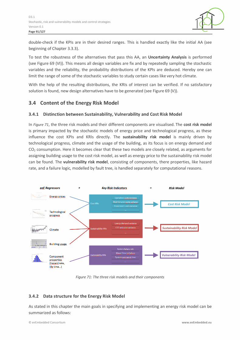
D3.1


Version 0.1

Page 91/127


double-check if the KPIs are in their desired ranges. This is handled exactly like the initial AA (see

beginning of Chapter 3.3.3).

To test the robustness of the alternatives that pass this AA, an Uncertainty Analysis is performed

(see Figure 69 (VI)). This means all design variables are fix and by repeatedly sampling the stochastic

variables and the reliability, the probability distributions of the KPIs are deduced. Hereby one can

limit the range of some of the stochastic variables to study certain cases like very hot climate.

With the help of the resulting distributions, the KRIs of interest can be verified. If no satisfactory

solution is found, new design alternatives have to be generated (see Figure 69 (V)).

3.4 Content of the Energy Risk Model

Distinction between Sustainability, Vulnerability and Cost Risk Model 3.4.1

In Figure 71, the three risk models and their different components are visualised. The cost risk model

is primary impacted by the stochastic models of energy price and technological progress, as these

influence the cost KPIs and KRIs directly. The sustainability risk model is mainly driven by

technological progress, climate and the usage of the building, as its focus is on energy demand and

CO2 consumption. Here it becomes clear that these two models are closely related, as arguments for

assigning building usage to the cost risk model, as well as energy price to the sustainability risk model

can be found. The vulnerability risk model, consisting of components, there properties, like hazard

rate, and a failure logic, modelled by fault tree, is handled separately for computational reasons.

Figure 71: The three risk models and their components

Data structure for the Energy Risk Model 3.4.2

As stated in this chapter the main goals in specifying and implementing an energy risk model can be

summarized as follows:

D3.1


Version 0.1

Page 92/127


- (1) provide uncertainty data to tools used for risk analysis - (2) support the identification of potential underperformances that can occur during the

building lifecycle - (3) provide a baseline for a risk-aware building design relying on the selection of proper

design alternatives and FM guidelines expressed as control strategies and maintenance plans In order to reach those goals the energy risk model must be elaborated in a way that it can be used

within the different domains specified in the eeEmbedded vision for a KPI-based holistic multi-

disciplinary design (Geißler et al., 2014). Those domains are differentiated between the design,

simulation and decision domains.

In order for the energy risk model to fulfil its first goal which is strongly related to the simulation

domain there is a need for a data structure providing the following features:

- representation of the uncertainty through stochastic variables - allocation of the stochastic variables to related design objects like building, building site,

building room, energy system component, etc. - representation of parameter variations for the alternative analyses and risk scenarios - representation of the variable samples necessary for the envisioned sensitivity and

uncertainty analyses - handling of the possible huge amount of parameter variations resulting from the data

requirements of such sensitivity and uncertainty analyses - easy exchange and mapping of the information for providing input data to several simulation

tools e.g. TRNSYS or R - easy configuration and population of the model

To allow for such features and to integrate the stochastic regressors identified in Chapter 2 into the

eeEmbedded overall multi-model data it has been chosen to reuse and further develop the

simulation matrix developed in the ISES project (Freudenberg et al., 2014). Indeed the simulation

matrix can provide a harmonised manner of capturing parameter variations for design parameters

(controllable parameters for the designer) as well as stochastic regressors (uncontrollable

parameters for the designer because of their stochastic nature). It is built using the eXtensible

Markup Language (XML) (W3C, 2015) that allows for a high level of interoperability. Indeed the XML

language is very flexible for creating, extending or modifying an information model quite easily. Also

XML as resource format is very spread in the software industry and can be easily transferred

between software applications. In view of that there exist sufficient tools for manipulating and

transforming XML information as it can be required for example by mapping the information into a

specific input format for a specific simulation tool. Moreover there exist different developer tools for

creating applications and user interfaces for an XML model. For all that reasons the simulation matrix

fits the previously listed requirements and can be used as an instance of the energy risk model for

simulation purpose.

The matrix is structured into two main sections as represented on Figure 72, one for describing

“Variances” and the second for describing “Combinations”. The “Variances” section defines all

desired variances of parameters, and the “Combinations” section contains links to the several

parameter variances and thus combines these variations defining particular building design

alternatives used as basis for simulation. In that way it is possible to make several combinations by

either varying one parameter each time or all parameters together. This possibility makes this

approach well suited to satisfy the specific requirements of different analysis methods, like for

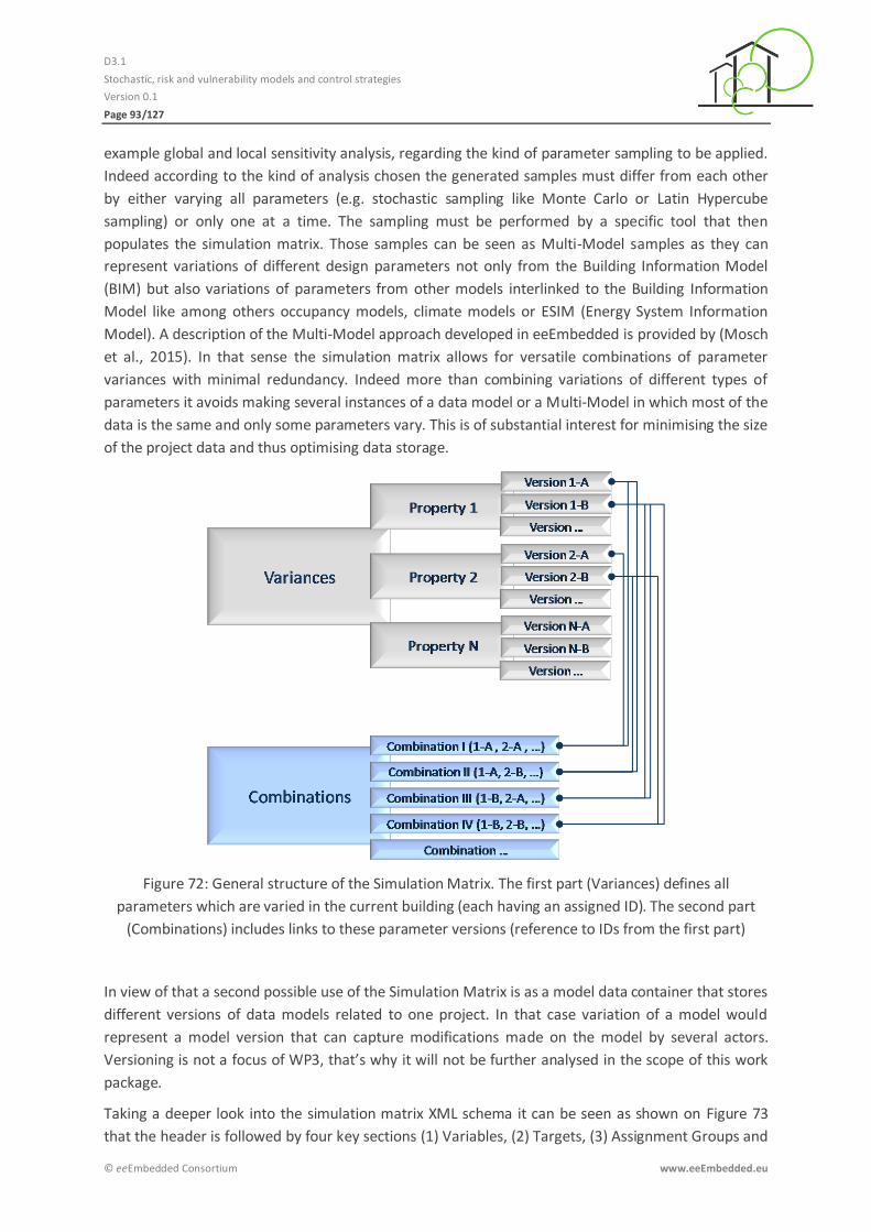
D3.1


Version 0.1

Page 93/127


example global and local sensitivity analysis, regarding the kind of parameter sampling to be applied.

Indeed according to the kind of analysis chosen the generated samples must differ from each other

by either varying all parameters (e.g. stochastic sampling like Monte Carlo or Latin Hypercube

sampling) or only one at a time. The sampling must be performed by a specific tool that then

populates the simulation matrix. Those samples can be seen as Multi-Model samples as they can

represent variations of different design parameters not only from the Building Information Model

(BIM) but also variations of parameters from other models interlinked to the Building Information

Model like among others occupancy models, climate models or ESIM (Energy System Information

Model). A description of the Multi-Model approach developed in eeEmbedded is provided by (Mosch

et al., 2015). In that sense the simulation matrix allows for versatile combinations of parameter

variances with minimal redundancy. Indeed more than combining variations of different types of

parameters it avoids making several instances of a data model or a Multi-Model in which most of the

data is the same and only some parameters vary. This is of substantial interest for minimising the size

of the project data and thus optimising data storage.

Figure 72: General structure of the Simulation Matrix. The first part (Variances) defines all

parameters which are varied in the current building (each having an assigned ID). The second part

(Combinations) includes links to these parameter versions (reference to IDs from the first part)

In view of that a second possible use of the Simulation Matrix is as a model data container that stores

different versions of data models related to one project. In that case variation of a model would

represent a model version that can capture modifications made on the model by several actors.

Versioning is not a focus of WP3, that’s why it will not be further analysed in the scope of this work

package.

Taking a deeper look into the simulation matrix XML schema it can be seen as shown on Figure 73

that the header is followed by four key sections (1) Variables, (2) Targets, (3) Assignment Groups and

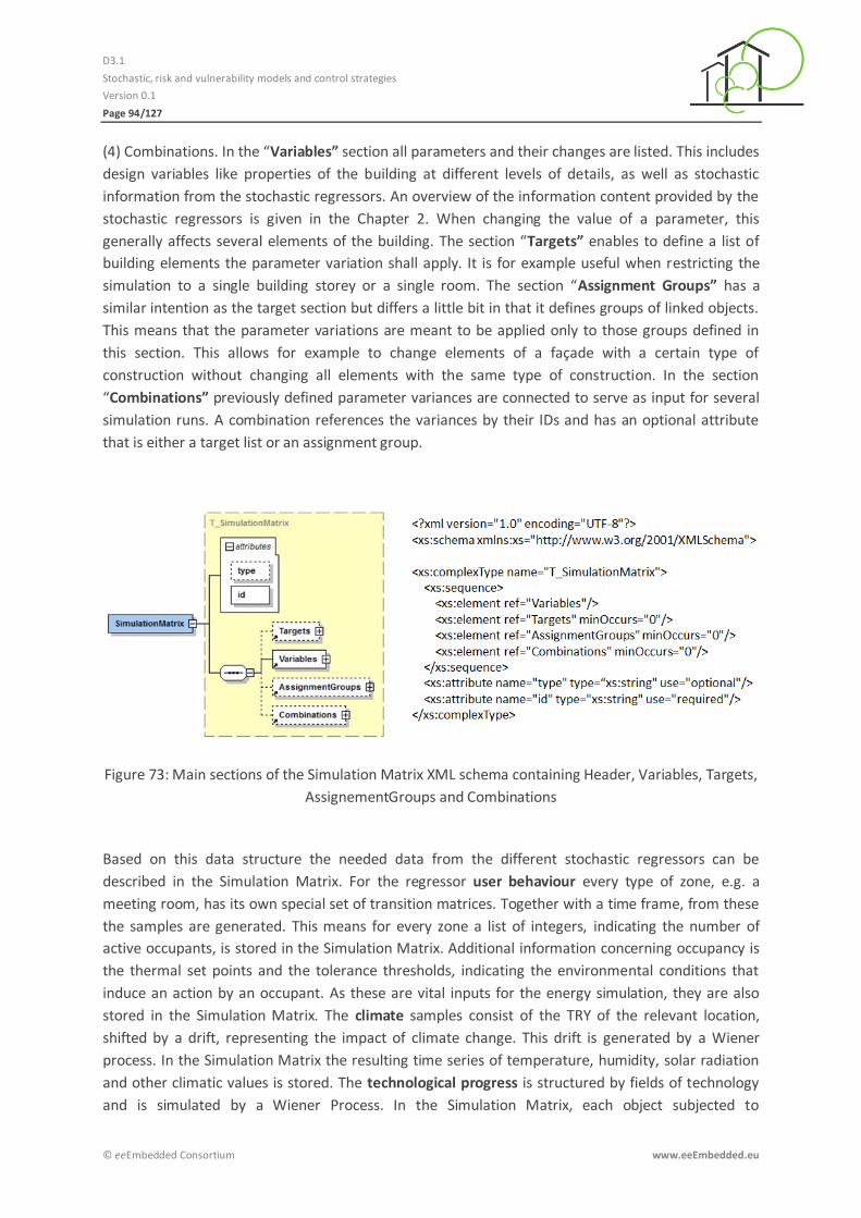
D3.1


Version 0.1

Page 94/127


(4) Combinations. In the “Variables” section all parameters and their changes are listed. This includes

design variables like properties of the building at different levels of details, as well as stochastic

information from the stochastic regressors. An overview of the information content provided by the

stochastic regressors is given in the Chapter 2. When changing the value of a parameter, this

generally affects several elements of the building. The section “Targets” enables to define a list of

building elements the parameter variation shall apply. It is for example useful when restricting the

simulation to a single building storey or a single room. The section “Assignment Groups” has a

similar intention as the target section but differs a little bit in that it defines groups of linked objects.

This means that the parameter variations are meant to be applied only to those groups defined in

this section. This allows for example to change elements of a façade with a certain type of

construction without changing all elements with the same type of construction. In the section

“Combinations” previously defined parameter variances are connected to serve as input for several

simulation runs. A combination references the variances by their IDs and has an optional attribute

that is either a target list or an assignment group.

Figure 73: Main sections of the Simulation Matrix XML schema containing Header, Variables, Targets,

AssignementGroups and Combinations

Based on this data structure the needed data from the different stochastic regressors can be

described in the Simulation Matrix. For the regressor user behaviour every type of zone, e.g. a

meeting room, has its own special set of transition matrices. Together with a time frame, from these

the samples are generated. This means for every zone a list of integers, indicating the number of

active occupants, is stored in the Simulation Matrix. Additional information concerning occupancy is

the thermal set points and the tolerance thresholds, indicating the environmental conditions that

induce an action by an occupant. As these are vital inputs for the energy simulation, they are also

stored in the Simulation Matrix. The climate samples consist of the TRY of the relevant location,

shifted by a drift, representing the impact of climate change. This drift is generated by a Wiener

process. In the Simulation Matrix the resulting time series of temperature, humidity, solar radiation

and other climatic values is stored. The technological progress is structured by fields of technology

and is simulated by a Wiener Process. In the Simulation Matrix, each object subjected to

D3.1


Version 0.1

Page 95/127


technological progress gets a time series assigned, consisting of values between 0 and 100, which

symbolise the increase in energy efficiency in percent in the component’s respective field. Energy

prices are simulated per source of energy via an ARIMA or a GARCH model. The Simulation Matrix

contains the outputs of these models, which is a time series of prices over a time frame for each

source of energy. The reliability model consists of several components and a failure logic in the form

of a fault tree. For each of these components the Simulation Matrix contains a hazard rate and, if

available additional information like repair times or times of scheduled maintenance.

As stated the simulation matrix has a strong relation to the simulation domain. Anyway the energy

risk model shall also interact with the design and decision domain in order to complete all the risk

management steps from the risk management cycle. Indeed as part of the risk identification step it is

of importance to identify first KRIs and related stochastic regressors, but also to allocate them to

elements of the engineering domains like the Building Information Model and the Energy System

Information Model as explained in (Pruvost et al., 2012). As an example the hazard rates that are part

of the vulnerability risk model shall be linked to corresponding components of the energy system. At

some point in the risk analysis process also the KRIs shall be interlinked to physical elements like the

building itself, a building zone or an energy subsystem. For that purpose an ontology can be used for

modelling the energy risk model in the context of the eeEmbedded Multi-Model and ontological

approach (Mosch et al., 2015). Ontology has the advantage to offer a very flexible structure thus

enabling to easily extend an engineering model with new information, like ESIM complemented with

hazard information. In ontology data interlinking is based on the concept of “triple” integrated in the

ontology format RDF that stands for Resource Description Format and the Web Ontology Language

OWL that implements its syntax (W3C, 2014). This concept used in the context of the Semantic Web

is very powerful for describing links with a high level of semantic. In that sense, more than

interlinking risk information with engineering elements, ontology could also be applied for modelling

risk scenarios like the ones described by fault trees. Another substantial interest in using ontology is

for the decision domain. Indeed OWL and its embedded description logic features allows for

reasoning on the overall data. More precisely there exist a set of modeller tools including generic

reasoners that apply the logical statements made in a model in order either to validate its

consistency, to complete its taxonomy or to create new links between its objects. In view of that it

seems possible to use ontology for linking risk responses like design alternatives or control strategies

to specific risk profiles expressed in terms of KRIs. This modelling strategy for integrating the energy

risk model into the design and decision domains are in a conceptual state and shall be further

analysed in future works.

D3.1


Version 0.1

Page 96/127


4 Control strategies

4.1 Intentions and introduction

The purpose of the Task 3.3 is to support the designer to set already in the design phase high level

control strategies which will be implemented in the operation phase, thereby enabling more efficient

Facility Management. Those control strategies shall provide a response to the actual vulnerability

and sustainability risk state of the building and respectively the energy system. They can rely on

templates like for example so called “management templates” used in BACS systems.

Templates can be of different categories like design templates, control templates and maintenance

templates. The design templates should be more the focus of Task 3.5. Indeed the goal of this task is

to help the designer make design alternatives which are based on the vulnerability, sustainability and

cost prognosis and which optimize the building design taking into consideration a trade-off between

targeted performances and investments. Task 3.3 put more emphasis on facility management aiming

at setting guidelines for building exploitation. In this sense control and maintenance templates are in

this section of interest. They have to be built upon the stochastic and risk models developed in Task

3.1 (Chapter 2) and Task 3.2 (Chapter 3).

The risk models by describing worst case scenarios and the critical system behaviour also define the

functions each template should provide. The purpose of the control templates is to specify different

ways the energy management system shall operate to avoid or fix those scenarios. For maintenance

purpose the templates can rely on the failure scenarios to specify maintenance plans. On the other

side, from the stochastic models it is possible to define time points at which specific control

strategies have to be implemented. Indeed as the stochastic model describes daily or yearly peak

loads the energy management system shall use specific control options in time accordingly.

Moreover early warnings can be specified helping the energy management system to recognize when

it shall implement a specific control option.

In order to be able to develop high level control strategy plans a classification of different control

strategies as well as an appropriated development methodology was elaborated. A general

classification of control strategies was specified and will be introduced in Section 4.2. In the

eeEmbedded context control strategies are divided in (1) operational control strategies, (2) short-

term control strategies and (3) long-term control strategies.

Control strategies in the context of eeEmbedded 4.1.1

The embedding of control strategies in the eeEmbedded context is described in this section. Figure 74

illustrates the integration of the control strategies in the eeeBIM Framework and the overall

stochastic approach.

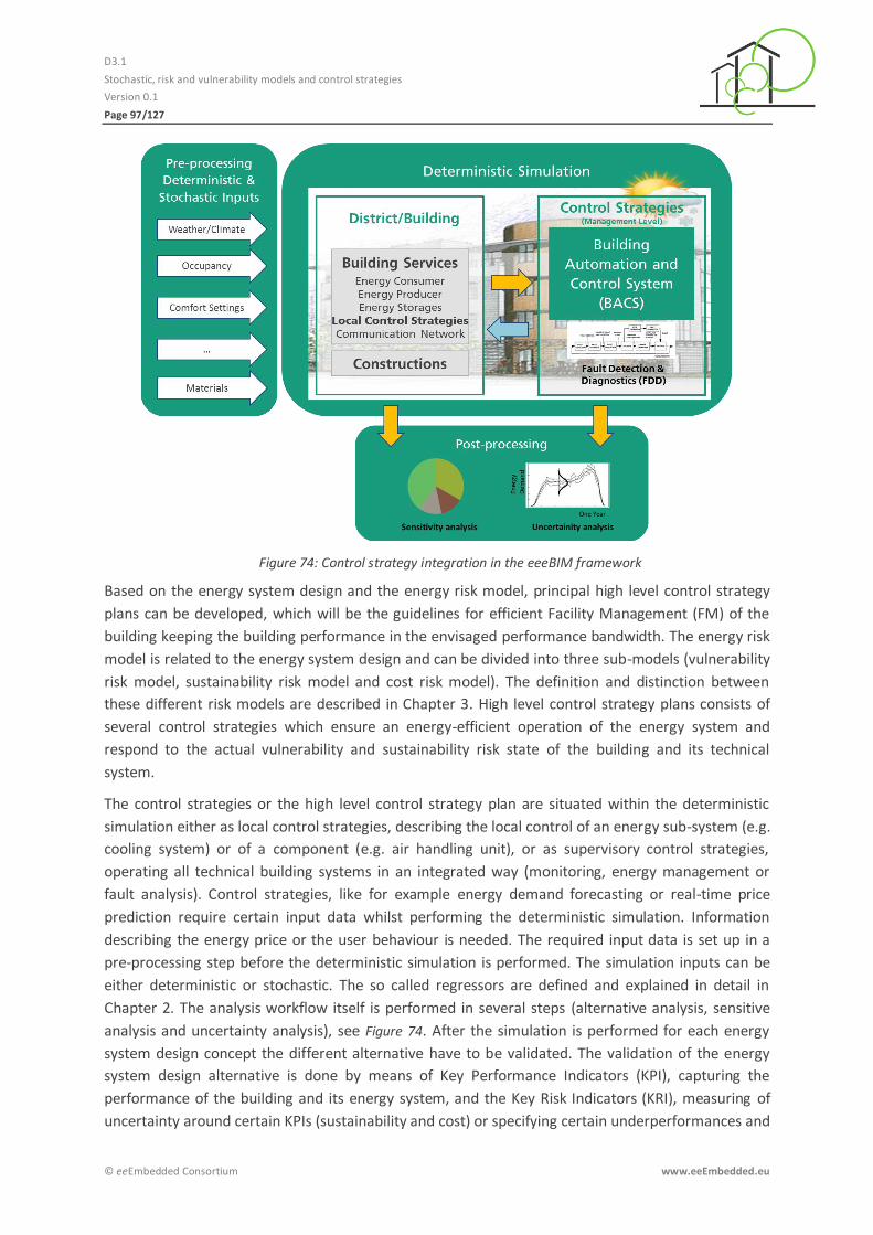
D3.1


Version 0.1

Page 97/127


Figure 74: Control strategy integration in the eeeBIM framework

Based on the energy system design and the energy risk model, principal high level control strategy

plans can be developed, which will be the guidelines for efficient Facility Management (FM) of the

building keeping the building performance in the envisaged performance bandwidth. The energy risk

model is related to the energy system design and can be divided into three sub-models (vulnerability

risk model, sustainability risk model and cost risk model). The definition and distinction between

these different risk models are described in Chapter 3. High level control strategy plans consists of

several control strategies which ensure an energy-efficient operation of the energy system and

respond to the actual vulnerability and sustainability risk state of the building and its technical

system.

The control strategies or the high level control strategy plan are situated within the deterministic

simulation either as local control strategies, describing the local control of an energy sub-system (e.g.

cooling system) or of a component (e.g. air handling unit), or as supervisory control strategies,

operating all technical building systems in an integrated way (monitoring, energy management or

fault analysis). Control strategies, like for example energy demand forecasting or real-time price

prediction require certain input data whilst performing the deterministic simulation. Information

describing the energy price or the user behaviour is needed. The required input data is set up in a

pre-processing step before the deterministic simulation is performed. The simulation inputs can be

either deterministic or stochastic. The so called regressors are defined and explained in detail in

Chapter 2. The analysis workflow itself is performed in several steps (alternative analysis, sensitive

analysis and uncertainty analysis), see Figure 74. After the simulation is performed for each energy

system design concept the different alternative have to be validated. The validation of the energy

system design alternative is done by means of Key Performance Indicators (KPI), capturing the

performance of the building and its energy system, and the Key Risk Indicators (KRI), measuring of

uncertainty around certain KPIs (sustainability and cost) or specifying certain underperformances and

D3.1


Version 0.1

Page 98/127


critical states of the energy system. Based on the simulation results captured by KPIs and KRIs it can

be decided whether the high level control strategy plans are suitable to keeping the building

performance in the envisaged performance bandwidth and avoid underperformances and critical

states of the energy system or whether the control strategy arrangement has to be reworked. After

updating the high level control strategy plan the deterministic simulation can be carried out again.

Existing standards describing control strategies 4.1.2

There exist already standards, norms or guidelines that cover partial aspects of control strategies in

the broadest sense. This section provides the state of the art according to control strategies and an

overview of the most related standards, norms or guidelines. The research on the related works

forms the basis for the classification in Chapter 4.2.

The standards EN 15232 and ISO 16484 as well as the German guideline VDI 3813 cover or deal with

functional descriptions of building, plant and room automation (BAC and/or RA functions

respectively). The mentioned functional descriptions are closely related to control strategies to

operate a building in an energy-efficient way while maintain the user comfort.

EN 15252 - Energy performance of buildings – Impact of Building Automation, Controls and

Building Management

This European standard EN 15252 provides a structured list of control, building automation and

technical building management functions which have an impact on the energy performance of

buildings and it technical building system (EN 15232). Using BAC Efficiency Classes (A, B, C, and D) of

building automation and technical building management functions the required building energy

performance can be achieved. The EN 15232 provides a promising basis for a functional description

of building automation and control system which can be covered by BACS models.

ISO 16484 - Building automation and control systems (BACS) -- Part 3: Functions

The international standard ISO 16484 provides a guideline for integrated planning and operation of

building automation and control systems. The standard defines BACS hardware, BAC functions and a

data communication protocol (BACnet) (ISO 16484-3, ISO 16484-5).

VDI 3813 - Building automation and control systems (BACS) - Room control functions (RA

functions)

The German guideline VDI 3813 applies to room control applications in the field of building services.

The guideline is defining room automation (RA) functions which are grouped into different function

groups (sensor functions, actuator functions, operator and display functions, application functions,

management functions, and service and diagnosis functions). Each RA function can be seen as a black

box including an interface description (VDI3813).

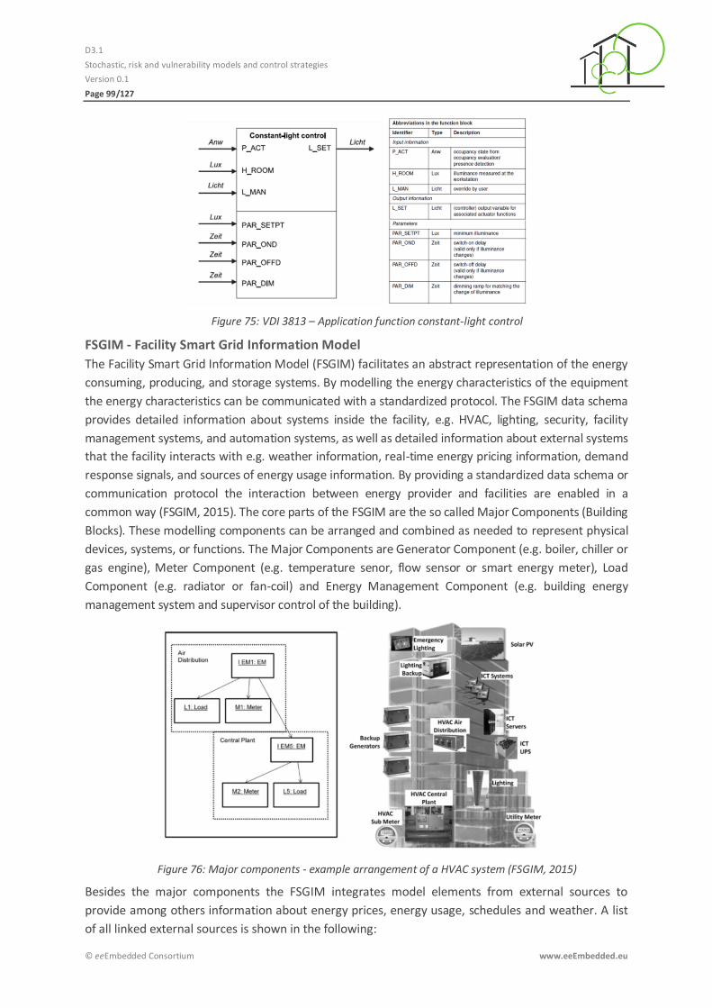
D3.1


Version 0.1

Page 99/127


Figure 75: VDI 3813 – Application function constant-light control

FSGIM - Facility Smart Grid Information Model

The Facility Smart Grid Information Model (FSGIM) facilitates an abstract representation of the energy

consuming, producing, and storage systems. By modelling the energy characteristics of the equipment

the energy characteristics can be communicated with a standardized protocol. The FSGIM data schema

provides detailed information about systems inside the facility, e.g. HVAC, lighting, security, facility

management systems, and automation systems, as well as detailed information about external systems

that the facility interacts with e.g. weather information, real-time energy pricing information, demand

response signals, and sources of energy usage information. By providing a standardized data schema or

communication protocol the interaction between energy provider and facilities are enabled in a

common way (FSGIM, 2015). The core parts of the FSGIM are the so called Major Components (Building

Blocks). These modelling components can be arranged and combined as needed to represent physical

devices, systems, or functions. The Major Components are Generator Component (e.g. boiler, chiller or

gas engine), Meter Component (e.g. temperature senor, flow sensor or smart energy meter), Load

Component (e.g. radiator or fan-coil) and Energy Management Component (e.g. building energy

management system and supervisor control of the building).

Figure 76: Major components - example arrangement of a HVAC system (FSGIM, 2015)

Besides the major components the FSGIM integrates model elements from external sources to

provide among others information about energy prices, energy usage, schedules and weather. A list

of all linked external sources is shown in the following:

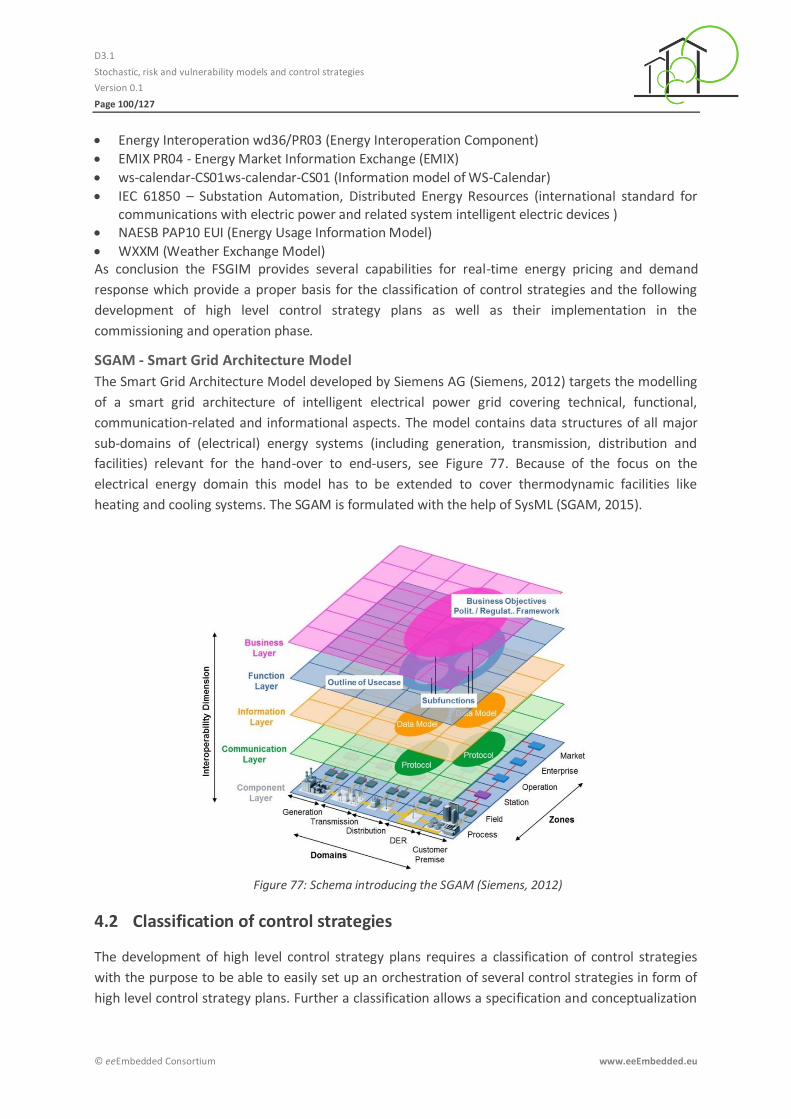
D3.1


Version 0.1

Page 100/127


Energy Interoperation wd36/PR03 (Energy Interoperation Component)

EMIX PR04 - Energy Market Information Exchange (EMIX)

ws-calendar-CS01ws-calendar-CS01 (Information model of WS-Calendar)

IEC 61850 – Substation Automation, Distributed Energy Resources (international standard for communications with electric power and related system intelligent electric devices )

NAESB PAP10 EUI (Energy Usage Information Model)

WXXM (Weather Exchange Model) As conclusion the FSGIM provides several capabilities for real-time energy pricing and demand

response which provide a proper basis for the classification of control strategies and the following

development of high level control strategy plans as well as their implementation in the

commissioning and operation phase.

SGAM - Smart Grid Architecture Model

The Smart Grid Architecture Model developed by Siemens AG (Siemens, 2012) targets the modelling

of a smart grid architecture of intelligent electrical power grid covering technical, functional,

communication-related and informational aspects. The model contains data structures of all major

sub-domains of (electrical) energy systems (including generation, transmission, distribution and

facilities) relevant for the hand-over to end-users, see Figure 77. Because of the focus on the

electrical energy domain this model has to be extended to cover thermodynamic facilities like

heating and cooling systems. The SGAM is formulated with the help of SysML (SGAM, 2015).

Figure 77: Schema introducing the SGAM (Siemens, 2012)

4.2 Classification of control strategies

The development of high level control strategy plans requires a classification of control strategies

with the purpose to be able to easily set up an orchestration of several control strategies in form of

high level control strategy plans. Further a classification allows a specification and conceptualization

D3.1


Version 0.1

Page 101/127


of those control strategies and their implementation using the generic eeTemplate (Zellner et al.

2015) and the ESIM data structure (Kaiser et al. 2015).

There are several possibilities to classify control strategies. Classifications according to 1)

management and application control strategies, 2) preventative, detective and corrective control

strategies, or 3) time horizon related control strategies are feasible. A classification into management

and application control strategies allows the distinction of specific applications, e.g. thermal control,

shading control, lighting control, on a lower level of the automation pyramid (see Figure 84), and

integrated management functionalities, e.g. monitoring, optimization and fault detection and

diagnosis (FDD), on a higher level of the automation pyramid. A classification into preventative,

detective and corrective control strategies is possible but not suitable, because most of the control

strategies can be assigned to each class. Finally a decision was taken to classify control strategies

according to the time horizon. A distinction into operational, short-term and long-term control

strategies to describe three main time horizons was chosen, in which each category can be further

decomposed into management and application control strategies (see Figure 87). An overview on

selected control strategies and their assignment to the elaborated classification is given in the

following sections.

Operational control strategies 4.2.1

In this section an overview on selected Operational Control Strategies is given and their usage in the

eeeBIM Framework and their influence on the potential energy system design or the integrated

building design respectively. This category summarizes control strategies that optimize the

operational behaviour of the energy system within a time horizon up to one day. The focus in the

operational phase lays on the Fault Detection and Diagnosis (FDD), Real-time pricing & energy

prediction and the Demand Response (Manual, Semi-Automated or Automated) for that each of

those are described a bit more in detail in the following.

4.2.1.1 Fault detection and diagnosis

Major attention will be paid to Fault Detection and Diagnosis (FDD) during the operation phase of the

energy system. Several faults can be identified, located, isolated and mostly avoided using a FDD

approach and hence the building performance can be increased. The following excerpt of possible

faults relevant to the eeeBIM Framework can be detected through FDD (Managan, 2013):

Equipment malfunction (such as broken/leaking valves, broken/stuck dampers, sensors out of calibration)

Systems with the wrong set points and operating schedules

Unintentional manual overrides

Dirty filters or strainers Pumps with throttled discharges

Short cycling of equipment

Excessive oscillation (hunting) of control points and/or control loop tuning needs

Incorrect fan and pump speeds, pressures, or low flow rates.

Improper building or space pressurizations (negative or positive)

Inefficient boiler combustion

Excessive building peak electrical demand

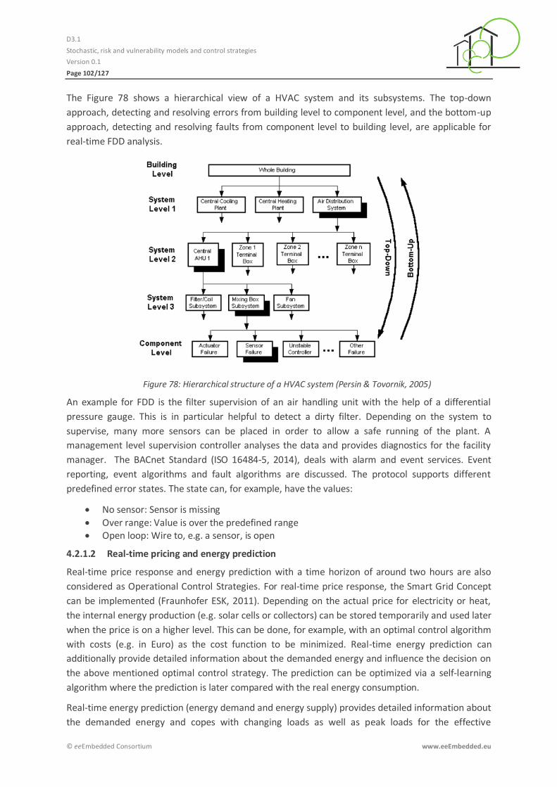
D3.1


Version 0.1

Page 102/127


The Figure 78 shows a hierarchical view of a HVAC system and its subsystems. The top-down

approach, detecting and resolving errors from building level to component level, and the bottom-up

approach, detecting and resolving faults from component level to building level, are applicable for

real-time FDD analysis.

Figure 78: Hierarchical structure of a HVAC system (Persin & Tovornik, 2005)

An example for FDD is the filter supervision of an air handling unit with the help of a differential

pressure gauge. This is in particular helpful to detect a dirty filter. Depending on the system to

supervise, many more sensors can be placed in order to allow a safe running of the plant. A

management level supervision controller analyses the data and provides diagnostics for the facility

manager. The BACnet Standard (ISO 16484-5, 2014), deals with alarm and event services. Event

reporting, event algorithms and fault algorithms are discussed. The protocol supports different

predefined error states. The state can, for example, have the values:

No sensor: Sensor is missing

Over range: Value is over the predefined range Open loop: Wire to, e.g. a sensor, is open

4.2.1.2 Real-time pricing and energy prediction

Real-time price response and energy prediction with a time horizon of around two hours are also

considered as Operational Control Strategies. For real-time price response, the Smart Grid Concept

can be implemented (Fraunhofer ESK, 2011). Depending on the actual price for electricity or heat,

the internal energy production (e.g. solar cells or collectors) can be stored temporarily and used later

when the price is on a higher level. This can be done, for example, with an optimal control algorithm

with costs (e.g. in Euro) as the cost function to be minimized. Real-time energy prediction can

additionally provide detailed information about the demanded energy and influence the decision on

the above mentioned optimal control strategy. The prediction can be optimized via a self-learning

algorithm where the prediction is later compared with the real energy consumption.

Real-time energy prediction (energy demand and energy supply) provides detailed information about

the demanded energy and copes with changing loads as well as peak loads for the effective

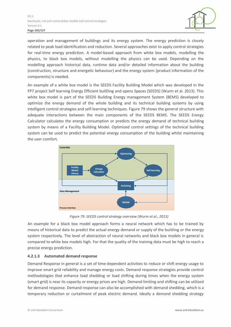
D3.1


Version 0.1

Page 103/127


operation and management of buildings and its energy system. The energy prediction is closely

related to peak load identification and reduction. Several approaches exist to apply control strategies

for real-time energy prediction. A model-based approach from white box models, modelling the

physics, to black box models, without modelling the physics can be used. Depending on the

modelling approach historical data, runtime data and/or detailed information about the building

(construction, structure and energetic behaviour) and the energy system (product information of the

components) is needed.

An example of a white box model is the SEEDS Facility Building Model which was developed in the

FP7 project Self learning Energy Efficient builDing and opens Spaces (SEEDS) (Wurm et al. 2013). This

white box model is part of the SEEDS Building Energy management System (BEMS) developed to

optimize the energy demand of the whole building and its technical building systems by using

intelligent control strategies and self-learning techniques. Figure 79 shows the general structure with

adequate interactions between the main components of the SEEDS BEMS. The SEEDS Energy

Calculator calculates the energy consumption or predicts the energy demand of technical building

system by means of a Facility Building Model. Optimized control settings of the technical building

system can be used to predict the potential energy consumption of the building whilst maintaining

the user comfort.

Controller

Data Management

Process Interface

Facility Model Library

Optimizing

Energy Calculator

Self-learning

Archiving

WISAN

Figure 79: SEEDS control strategy overview (Wurm et al., 2013)

An example for a black box model approach forms a neural network which has to be trained by

means of historical data to predict the actual energy demand or supply of the building or the energy

system respectively. The level of abstraction of neural networks and black box models in general is

compared to white box models high. For that the quality of the training data must be high to reach a

precise energy prediction.

4.2.1.3 Automated demand response

Demand Response in general is a set of time‐dependent activities to reduce or shift energy usage to

improve smart grid reliability and manage energy costs. Demand response strategies provide control

methodologies that enhance load shedding or load shifting during times when the energy system

(smart grid) is near its capacity or energy prices are high. Demand limiting and shifting can be utilized

for demand response. Demand response can also be accomplished with demand shedding, which is a

temporary reduction or curtailment of peak electric demand. Ideally a demand shedding strategy

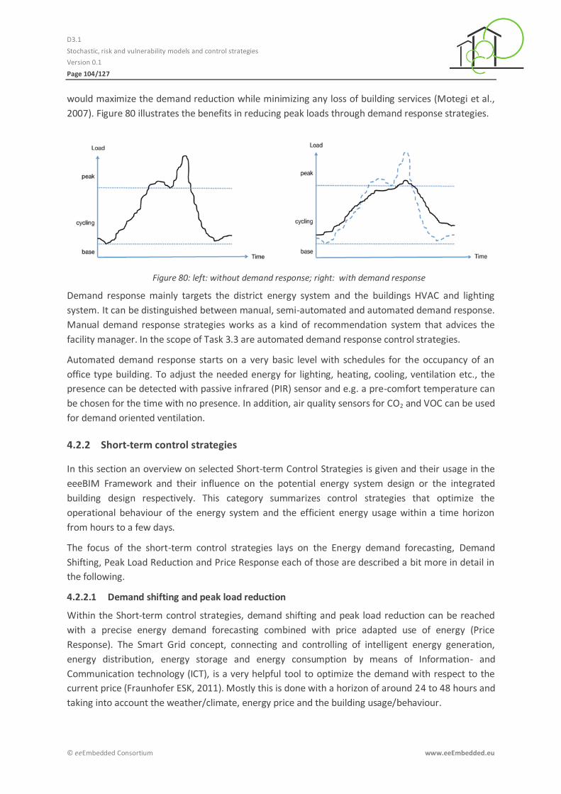
D3.1


Version 0.1

Page 104/127


would maximize the demand reduction while minimizing any loss of building services (Motegi et al.,

2007). Figure 80 illustrates the benefits in reducing peak loads through demand response strategies.

Figure 80: left: without demand response; right: with demand response

Demand response mainly targets the district energy system and the buildings HVAC and lighting

system. It can be distinguished between manual, semi-automated and automated demand response.

Manual demand response strategies works as a kind of recommendation system that advices the

facility manager. In the scope of Task 3.3 are automated demand response control strategies.

Automated demand response starts on a very basic level with schedules for the occupancy of an

office type building. To adjust the needed energy for lighting, heating, cooling, ventilation etc., the

presence can be detected with passive infrared (PIR) sensor and e.g. a pre-comfort temperature can

be chosen for the time with no presence. In addition, air quality sensors for CO2 and VOC can be used

for demand oriented ventilation.

Short-term control strategies 4.2.2

In this section an overview on selected Short-term Control Strategies is given and their usage in the

eeeBIM Framework and their influence on the potential energy system design or the integrated

building design respectively. This category summarizes control strategies that optimize the

operational behaviour of the energy system and the efficient energy usage within a time horizon

from hours to a few days.

The focus of the short-term control strategies lays on the Energy demand forecasting, Demand

Shifting, Peak Load Reduction and Price Response each of those are described a bit more in detail in

the following.

4.2.2.1 Demand shifting and peak load reduction

Within the Short-term control strategies, demand shifting and peak load reduction can be reached

with a precise energy demand forecasting combined with price adapted use of energy (Price

Response). The Smart Grid concept, connecting and controlling of intelligent energy generation,

energy distribution, energy storage and energy consumption by means of Information- and

Communication technology (ICT), is a very helpful tool to optimize the demand with respect to the

current price (Fraunhofer ESK, 2011). Mostly this is done with a horizon of around 24 to 48 hours and

taking into account the weather/climate, energy price and the building usage/behaviour.

D3.1


Version 0.1

Page 105/127


Another example for demand shifting control strategies is the intelligent usage of the thermal mass

of the building. Pre‐cooling the thermal mass of the building can be used to shift the cooling demand

and to reduce the peak load. In summer, the building mass can be cooled during the night to reduce

the cooling load in the day hours. As a result, the cooling load is shifted in time and the peak demand

is reduced. The building mass can be cooled most effectively during unoccupied hours because it is

possible to relax the comfort constraints (Motegi et al., 2007). Furthermore a pre-heating of the

building thermal mass is possible to avoid peak loads due to demand shifting.

4.2.2.2 Energy demand forecasting

The energy consumption for heating/cooling as well as electricity of a building is influenced by

several internal and external factors. A categorization into several main clusters of these factors was

given in Chapter 2.2.1. The main clusters among others are for instance the building

usage/occupancy, the energy price and the weather/climate.

The energy demand forecasting as control strategy can be assigned to the short-term as well as to

long-term control strategies. In the context of short-term strategies the energy prediction takes place

for hours up to a few days. The energy demand forecasting can be design model based, where e.g.

the weather input and a presence scheduler are two necessary inputs for calculating the demanded

energy. Appropriated approaches to predict the energy demand were introduced in Chapter 2.2.

4.2.2.3 Price response

Price-based demand response refers to changes in usage by customers in response to changes in the

prices they pay and include critical-peak pricing, real-time pricing and time-of-use rates. If the price

differentials between hours or time periods are significant, customers can respond to the price

structure with significant changes in energy use, reducing their energy costs if they adjust the timing

of their energy usage to take advantage of lower-priced periods and avoid consuming when prices

are higher.

In general prices are important, both to energy users and energy producers. Prices response provides

the opportunity for energy users to voluntarily reduce their energy consumption when prices rise in

the regional wholesale energy market. In open energy markets, prices are volatile and typically rise

fast. In the wholesale market prices can fluctuate in minutes due to peak demand events.

As already mentioned price response strategies include time-of-use rates and critical-peak pricing. In

(DOE, 2006) both strategies are described as follows:

Time-of-use (TOU): a rate with different unit prices for usage during different blocks of time, usually

defined for a 24 hour day. TOU rates reflect the average cost of generating and delivering power

during those time periods.

Real-time pricing (RTP): a rate in which the price for electricity typically fluctuates hourly reflecting

changes in the wholesale price of electricity. Customers are typically notified of RTP prices on a day-

ahead or hour-ahead basis.

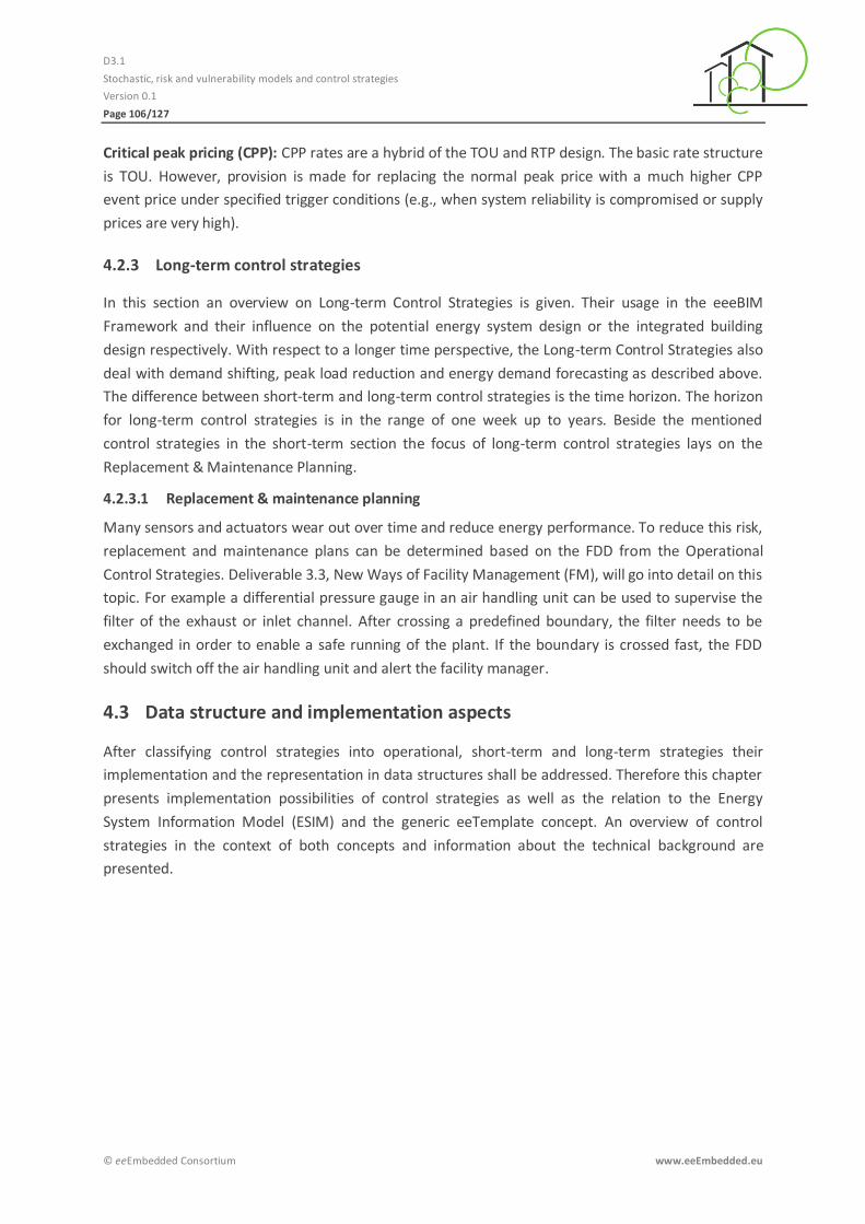
D3.1


Version 0.1

Page 106/127


Critical peak pricing (CPP): CPP rates are a hybrid of the TOU and RTP design. The basic rate structure

is TOU. However, provision is made for replacing the normal peak price with a much higher CPP

event price under specified trigger conditions (e.g., when system reliability is compromised or supply

prices are very high).

Long-term control strategies 4.2.3

In this section an overview on Long-term Control Strategies is given. Their usage in the eeeBIM

Framework and their influence on the potential energy system design or the integrated building

design respectively. With respect to a longer time perspective, the Long-term Control Strategies also

deal with demand shifting, peak load reduction and energy demand forecasting as described above.

The difference between short-term and long-term control strategies is the time horizon. The horizon

for long-term control strategies is in the range of one week up to years. Beside the mentioned

control strategies in the short-term section the focus of long-term control strategies lays on the

Replacement & Maintenance Planning.

4.2.3.1 Replacement & maintenance planning

Many sensors and actuators wear out over time and reduce energy performance. To reduce this risk,

replacement and maintenance plans can be determined based on the FDD from the Operational

Control Strategies. Deliverable 3.3, New Ways of Facility Management (FM), will go into detail on this

topic. For example a differential pressure gauge in an air handling unit can be used to supervise the

filter of the exhaust or inlet channel. After crossing a predefined boundary, the filter needs to be

exchanged in order to enable a safe running of the plant. If the boundary is crossed fast, the FDD

should switch off the air handling unit and alert the facility manager.

4.3 Data structure and implementation aspects

After classifying control strategies into operational, short-term and long-term strategies their

implementation and the representation in data structures shall be addressed. Therefore this chapter

presents implementation possibilities of control strategies as well as the relation to the Energy

System Information Model (ESIM) and the generic eeTemplate concept. An overview of control

strategies in the context of both concepts and information about the technical background are

presented.

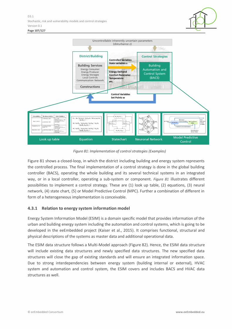
D3.1


Version 0.1

Page 107/127


Figure 81: Implementation of control strategies (Examples)

Figure 81 shows a closed-loop, in which the district including building and energy system represents

the controlled process. The final implementation of a control strategy is done in the global building

controller (BACS), operating the whole building and its several technical systems in an integrated

way, or in a local controller, operating a sub-system or component. Figure 81 illustrates different

possibilities to implement a control strategy. These are (1) look up table, (2) equations, (3) neural

network, (4) state chart, (5) or Model Predictive Control (MPC). Further a combination of different in

form of a heterogeneous implementation is conceivable.

Relation to energy system information model 4.3.1

Energy System Information Model (ESIM) is a domain specific model that provides information of the

urban and building energy system including the automation and control systems, which is going to be

developed in the eeEmbedded project (Kaiser et al., 2015). It comprises functional, structural and

physical descriptions of the systems as master data and additional operational data.

The ESIM data structure follows a Multi-Model approach (Figure 82). Hence, the ESIM data structure

will include existing data structures and newly specified data structures. The new specified data

structures will close the gap of existing standards and will ensure an integrated information space.

Due to strong interdependencies between energy system (building internal or external), HVAC

system and automation and control system, the ESIM covers and includes BACS and HVAC data

structures as well.

D3.1


Version 0.1

Page 108/127


Figure 82: ESIM relation to other domain models

Beside existing data structure the ESIM owns core parts which contain the following identified main

aspects of energy systems: (1) energy sources, (2) transformation facilities, (3) distribution systems,

(4) storage systems, (5) automation and control systems (ACS), (6) consumption / usage information

and (6) energy-related information exchange. The Figure 83 illustrates the core part related structure

in a high-level manner. A detailed description of the ESIM core parts are given in (Kaiser et al., 2015).

The representation of control strategies (operational, short-term and long-term strategies) takes

place in the automation and control system part. In general this part covers different physical types

of ACS, sub-systems and component to describe the orchestration of production/transformation,

distribution, storage and use of energy and media. Further behavioural and functional information

are covered. There exists a strong relation between control strategies introduced in Chapter 4.2, and

functions (RA/BAC functions). To fulfil a specific control strategy a corresponding set of

functionalities are needed.

Figure 83: ESIM Core Parts – Automation and Control System

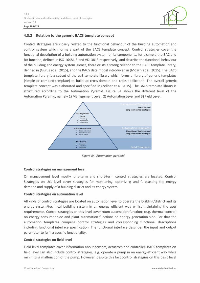
D3.1


Version 0.1

Page 109/127


Relation to the generic BACS template concept 4.3.2

Control strategies are closely related to the functional behaviour of the building automation and

control system which forms a part of the BACS template concept. Control strategies cover the

functional description of a building automation system or its components, for example the BAC and

RA function, defined in ISO 16484-3 and VDI 3813 respectively, and describe the functional behaviour

of the building and energy system. Hence, there exists a strong relation to the BACS template library,

defined in (Guruz et al. 2015), and the BACS data model introduced in (Mosch et al. 2015). The BACS

template library is a subset of the eeE template library which forms a library of generic templates

(simple or complex template) to build-up cross-domain and cross-application. The overall generic

template concept was elaborated and specified in (Zellner et al. 2015). The BACS template library is

structured according to the Automation Pyramid. Figure 84 shows the different level of the

Automation Pyramid, namely 1) Management Level, 2) Automation Level and 3) Field Level.

Figure 84: Automation pyramid

Control strategies on management level

On management level mostly long-term and short-term control strategies are located. Control

Strategies on this level cover strategies for monitoring, optimizing and forecasting the energy

demand and supply of a building district and its energy system.

Control strategies on automation level

All kinds of control strategies are located on automation level to operate the building/district and its

energy system/technical building system in an energy efficient way whilst maintaining the user

requirements. Control strategies on this level cover room automation functions (e.g. thermal control)

on energy consumer side and plant automation functions on energy generation side. For that the

automation templates comprise control strategies and corresponding functional descriptions

including functional interface specification. The functional interface describes the input and output

parameter to fulfil a specific functionality.

Control strategies on field level

Field level templates cover information about sensors, actuators and controller. BACS templates on

field level can also include control strategies, e.g. operate a pump in an energy-efficient way while

minimizing malfunction of the pump. However, despite this fact control strategies on this basic level

D3.1


Version 0.1

Page 110/127


are not in scope of Task 3.3, because the purpose is the development of high level control strategy

Plans which serve as basis for the implementation in the operation phase enabling more efficient

Facility Management (FM). Although control strategies related to maintenance are important on

BACS field level. For maintenance purpose the control strategies can rely on the failure scenarios to

specify maintenance plans.

The following example shall show the relationship between control strategies and BACS templates.

The example bases on the simple building demonstrator which is introduced in Chapter 4.4.2.

The Figure 85 presents the corresponding BACS management template, namely Simple Building

Control, and its interlinkages to other BACS templates. The Simple Building Control covers all

information to plan, simulate and later to operate a building in an energy efficient manner whilst

maintaining the user comfort. Therefore, the management template comprises several automation

templates that cover control strategies for thermal comfort control on energy consumer side and

control strategies for heating and cooling plants on energy producer side. Besides the control

strategy the corresponding room automation (RA) functions and building automation and control

(BAC) functions including functional interface description are covered. Further Simple Building

Control Template comprises BACS equipment information for controller, sensors and actuators. In

order to validate the BACS design solution, based on the Simple Building Control Template,

information about building usage as well as weather and climate conditions are provided. As it can

be seen the management template also contains a kind of control strategy plan. The Building Control

Strategy template comprises control strategies for real-time pricing, energy forecasting and

replacement & maintenance planning. Each of these templates includes application and

management functions which are needed to realize the appropriated control strategy. Depending on

the application or management function respectively a functional interface description is given that

has to be implemented to fulfil a specific function (BAC/RA function).

Figure 86 presents the BACS automation template Thermal Control, included in BACS management

template above, a bit more in detail. The illustrated automation template can be either a part of a

management template or can be used on its own. The Thermal Control template comprises BACS

field templates covering sensor-related information (Temperature Sensor) and data structures

covering the local controls of the technical system (Fan-Coil Control). Both BACS Field Templates can

contain control strategies as well, e.g. replacement and maintenance plans. Further the control

strategy (Thermal Control Strategy) covering the RA functions to fulfil the thermal control of a spatial

structure is described by the template content. The presented Automation Template also covers

domain-independent information like space usage, weather or lifecycle cost.

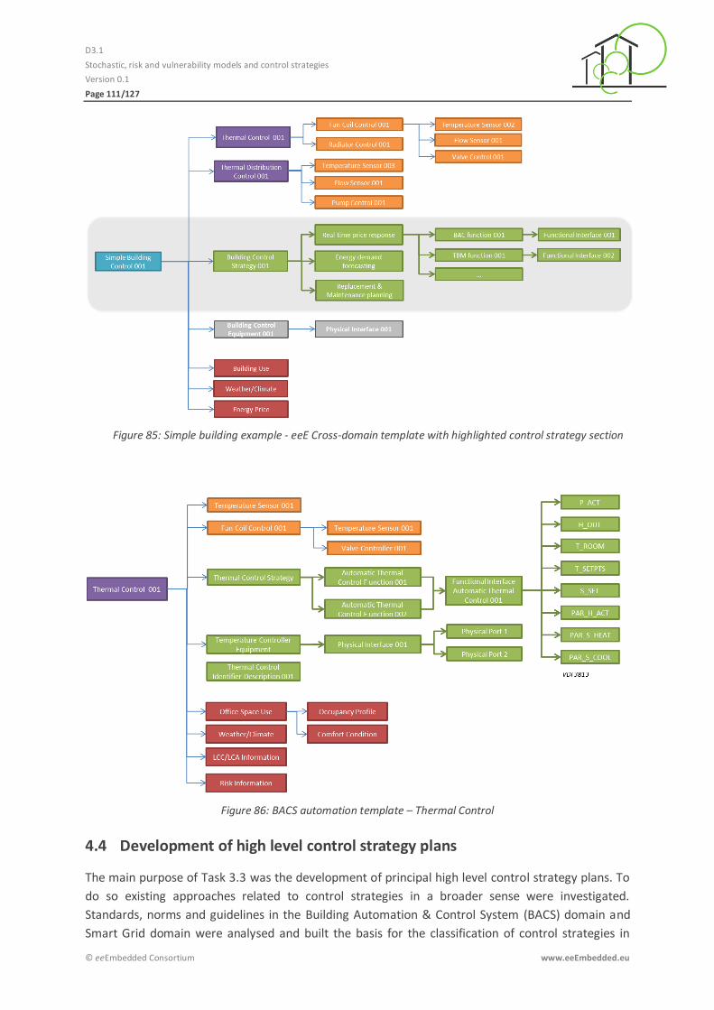
D3.1


Version 0.1

Page 111/127


Figure 85: Simple building example - eeE Cross-domain template with highlighted control strategy section

Figure 86: BACS automation template – Thermal Control

4.4 Development of high level control strategy plans

The main purpose of Task 3.3 was the development of principal high level control strategy plans. To

do so existing approaches related to control strategies in a broader sense were investigated.

Standards, norms and guidelines in the Building Automation & Control System (BACS) domain and

Smart Grid domain were analysed and built the basis for the classification of control strategies in

D3.1


Version 0.1

Page 112/127


Chapter 4.2. The following chapter presents the basic methodology on how to develop high level

control strategy plans, their integration in the overall stochastic analysis framework as well as the

elaboration of such principal high level control strategy plans on a simple example.

Development methodology 4.4.1

Based on the energy system design and the energy risk model, high level control strategy plans are

going to be developed. To be able to design these control strategy plans in a manner way an

appropriated development methodology is needed. The development of Control Strategy Plans is

part of the design process introduced in Chapter 4.2. The schematic workflow for designing,

analysing as well as optimizing the energy generation and distribution system taking into account a

broad variety of influencing factors while elaborating a sophisticated and state-of the art as well as

future-proof energy system was introduced in Figure 3. A set of appropriate control strategies can be

selected in several working steps and their subtasks to operate the elaborated energy system or

partial energy systems, e.g. energy generation or distribution network. For that the energy system

design can be simulated including the high level control strategy plans increase the performance or

to identify optimization potential of the design alternative.

However, these high level control strategy plans developed according to the defined methodology

are not necessarily the control strategy plans which are used in the commissioning and operation

phase, but they should serve as their baselines for the real building and energy system operation to

ensure energy optimized performance whilst maintaining the user comfort.

The Figure 87 illustrates the elaboration of high level control strategy plans. As already mentioned an

energy system design variant and the related risk model form the basis. Therefore, the elaboration of

high level control strategy plans follows the overall structure of finding variants and alternatives

within the eeEmbedded project. Based on different BACS requirements, Key Design Parameter (KDP)

to-be, Operational Control Strategies are defined. This control strategies and further KDP to-be form

the baseline for short-term control strategies which again result in long-term control strategies.

Possible KDPs to-be are maintenance intervals, invest costs, lifecycle costs (LCC), user comfort or

energy efficiency (see Figure 87). As an example, with the demand of low LCC, a high user comfort

and predictable maintenance intervals with the risk of higher invest cost, additional sensors for FDD

guarantee a safe running from operational perspective. Having a sustainable FDD as a baseline,

detailed and predictable replacement/maintenance plans can be developed.

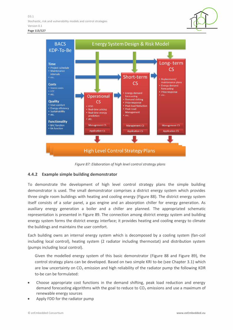
D3.1


Version 0.1

Page 113/127


Figure 87: Elaboration of high level control strategy plans

Example simple building demonstrator 4.4.2

To demonstrate the development of high level control strategy plans the simple building

demonstrator is used. The small demonstrator comprises a district energy system which provides

three single room buildings with heating and cooling energy (Figure 88). The district energy system

itself consists of a solar panel, a gas engine and an absorption chiller for energy generation. As

auxiliary energy generation a boiler and a chiller are planned. The appropriated schematic

representation is presented in Figure 89. The connection among district energy system and building

energy system forms the district energy interface; it provides heating and cooling energy to climate

the buildings and maintains the user comfort.

Each building owns an internal energy system which is decomposed by a cooling system (fan-coil

including local control), heating system (2 radiator including thermostat) and distribution system

(pumps including local control).

Given the modelled energy system of this basic demonstrator (Figure 88 and Figure 89), the

control strategy plans can be developed. Based on two simple KRI to-be (see Chapter 3.1) which

are low uncertainty on CO2 emission and high reliability of the radiator pump the following KDR

to-be can be formulated:

Choose appropriate cost functions in the demand shifting, peak load reduction and energy demand forecasting algorithms with the goal to reduce to CO2 emissions and use a maximum of renewable energy sources

Apply FDD for the radiator pump

D3.1


Version 0.1

Page 114/127


Based on these KDR to-be, specific BACS templates are chosen and integrated in the model. In a next

step, the workflow from the previous chapters starts. This means, on a high level perspective, sample

generation, deterministic simulations including the control strategies, post processing and analysis of

the data. After this step, the KRI as-is are available and can be compared to the targeted KRI to-be. If

the performance is sufficient, the next design steps starts. Otherwise, the KDR to-be have to be

adapted in order to perform better in terms of KRI as-is.

Figure 88: Simple building demonstrator

Figure 89: Schematic representation district energy system

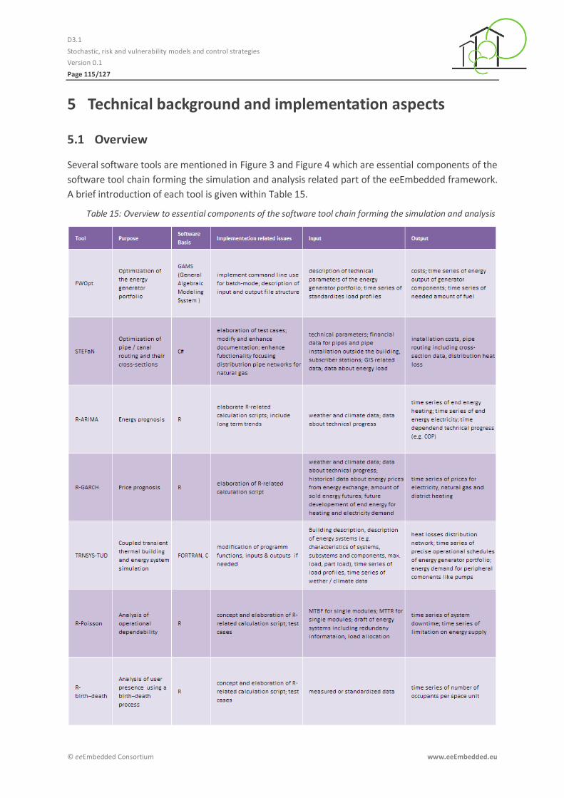
D3.1


Version 0.1

Page 115/127


5 Technical background and implementation aspects

5.1 Overview

Several software tools are mentioned in Figure 3 and Figure 4 which are essential components of the

software tool chain forming the simulation and analysis related part of the eeEmbedded framework.

A brief introduction of each tool is given within Table 15.

Table 15: Overview to essential components of the software tool chain forming the simulation and analysis

D3.1


Version 0.1

Page 116/127


5.2 Brief introduction of the used software tools

The following chapters are providing more detailed information about each tool.

R 5.2.1

The software package R is described as “language and environment for statistical computing and

graphics … providing a wide variety of statistical (linear and nonlinear modelling, classical statistical

tests, time-series analysis, classification, clustering …) and graphical techniques” (R Project, 2015). R

is distributed as free software under the Free Software Foundation’s GNU General Public License and

available for all common software platforms. Regarding the stochastic related tasks within the

workflow of the analysis approach of the eeEmbedded project R will be used on certain stages within

the tool chain.

STEFaN 5.2.2

Within the software tool chain which is used to design and optimise the energy system - especially

the energy generation part, storages and distribution networks - the software tool STEFaN (Gnüchtel,

2013a) helps to optimise the topology of the distribution network taking into account the subscribers

maximum thermal load, their geographical position and additional circumstances which act as

geographical, infrastructural of financial hindrances, e.g. rivers, streets, pedestrian walkways,

buildings or special conditions within the ground. The tools is using a GIS data set which contains

information about the position of buildings and other infrastructure elements. This information is

extended with data describing the subscriber’s position, the maximum thermal load and the load

profiles. As a result the optimised topology of the distribution network based on financial and

operational issues is processed, see Figure 90.

The software tool was developed from eeEmbedded project partner TUD-IET and is currently running

on Windows platforms. The solution STEFaN is publicly available for free in binary format without

support1. For commercial use a registration is required. Figure 91 shows a network topology as result

of an optimisation run.

1 http://tu-dresden.de/die_tu_dresden/fakultaeten/fakultaet_maschinenwesen/iet/ew/forschung_und_projekte/mldh/download_mldh

Figure 90: Software tool STEFaN – covering the enhancement of GIS data for modelling the buildings, topology and infrastructure beside the site and the distribution pipe system and subscriber’s position

http://www.gnu.org/

http://www.r-project.org/COPYING

http://tu-dresden.de/die_tu_dresden/fakultaeten/fakultaet_maschinenwesen/iet/ew/forschung_und_projekte/mldh/download_mldh

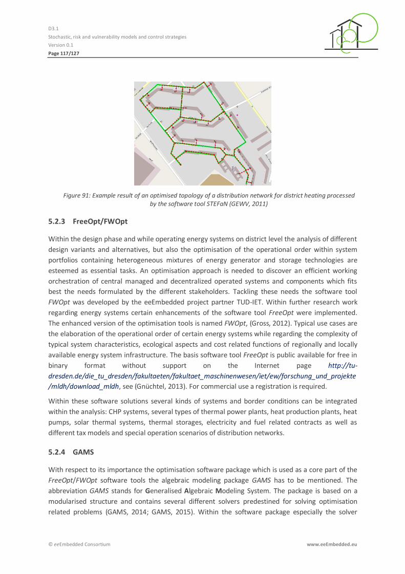
D3.1


Version 0.1

Page 117/127


Figure 91: Example result of an optimised topology of a distribution network for district heating processed by the software tool STEFaN (GEWV, 2011)

FreeOpt/FWOpt 5.2.3

Within the design phase and while operating energy systems on district level the analysis of different

design variants and alternatives, but also the optimisation of the operational order within system

portfolios containing heterogeneous mixtures of energy generator and storage technologies are

esteemed as essential tasks. An optimisation approach is needed to discover an efficient working

orchestration of central managed and decentralized operated systems and components which fits

best the needs formulated by the different stakeholders. Tackling these needs the software tool

FWOpt was developed by the eeEmbedded project partner TUD-IET. Within further research work

regarding energy systems certain enhancements of the software tool FreeOpt were implemented.

The enhanced version of the optimisation tools is named FWOpt, (Gross, 2012). Typical use cases are

the elaboration of the operational order of certain energy systems while regarding the complexity of

typical system characteristics, ecological aspects and cost related functions of regionally and locally

available energy system infrastructure. The basis software tool FreeOpt is public available for free in

binary format without support on the Internet page http://tu-

dresden.de/die_tu_dresden/fakultaeten/fakultaet_maschinenwesen/iet/ew/forschung_und_projekte

/mldh/download_mldh, see (Gnüchtel, 2013). For commercial use a registration is required.

Within these software solutions several kinds of systems and border conditions can be integrated

within the analysis: CHP systems, several types of thermal power plants, heat production plants, heat

pumps, solar thermal systems, thermal storages, electricity and fuel related contracts as well as

different tax models and special operation scenarios of distribution networks.

GAMS 5.2.4

With respect to its importance the optimisation software package which is used as a core part of the

FreeOpt/FWOpt software tools the algebraic modeling package GAMS has to be mentioned. The

abbreviation GAMS stands for Generalised Algebraic Modeling System. The package is based on a

modularised structure and contains several different solvers predestined for solving optimisation

related problems (GAMS, 2014; GAMS, 2015). Within the software package especially the solver




D3.1


Version 0.1

Page 118/127


CPLEX will be used for optimisation purposes. GAMS is available for all common operation software

platforms and under certain license models.

TRNSYS-TUD 5.2.5

TRNSYS is the abbreviation for TRaNsient SYstem Simulation program which is developed by the

University of Wisconsin in Madison, USA for approximately 35 years. This simulation package is

focused on modeling energy systems and related buildings. It is based on a modularised concept

which provides a high level of flexibility when analysing various kinds of energy systems while

involving peripheral conditions and related phenomena. Because of the modularised approach of the

software design experienced users have the possibility to add their own written software code to the

core software parts to process simulation according to their individual tasks. Parts of the software

code are distributed as source code, other (core) parts are available only as binaries.

Within the eeEmbedded project TRNSYS acts as a common placeholder for software systems used for

transient thermal building and energy system simulation and similar purposes. Within a productive

environment based on research results of the eeEmbedded project a comparable tool with similar

functionality could be used.

The eeEmbedded project partner TUD-IET started the development of its own individual software

modules for TRNSYS in 1994. Since this time more and more new simulation modules were added or

existing modules were re-shaped respectively adapted to support the special tasks within research

projects. Because of the high rate of newly developed software modules and approaches which are

unique compared with the software setup which is available as commercial solution the suffix TUD

was added to the original trademark TRNSYS to indicate the difference between the commercial tool

and the research-orientated solution TRNSYS-TUD. The additional or modified software modules

developed by TUD-IET are not available for purchase or free distribution.

D3.1


Version 0.1

Page 119/127


6 Conclusions

Chapter 1 contains an overview about the intensions related to the usage of stochastic approaches

within the design process in general and related to the description of work (DOW) of the

eeEmbedded project. Within this chapter typical design steps within the workflow of energy system

design are described. A systematisation of the involved stochastic models is given and linked to

appropriate tasks within the design workflow.

Chapter 2 provides one main subchapters dedicated to the forecasting of energy consumption within

the building lifecycle. With respect to the expected duration of the lifecycle certain regressors were

identified and discussed in the context of their individual stochastic character and importance to the

energy consumption. As main regressors are mentioned user behaviour, climate trend, energy price

as well as technological progress. Besides the energy consumption certain aspects related to a

vulnerability analysis within the design process of (energy) systems is discussed within a second

subchapter. Especially a reliability/dependability analysis could support the decision making domain

when comparing different energy system concepts. Unfortunately in the construction and energy

system domain there is no broad data base available which contains reliability/dependability related

values for processing a high detailed analysis. Because of the strong relationship to the operational

phase of a building the aspects malfunction and underperformance are mentioned but not discussed

in a detailed manner.

In Chapter 3 the energy risk model, consisting of the sustainability risk model, the vulnerability risk

model and the cost risk model, has been established. Each of these submodels has been described

considering the concepts they rely on, their content and their structure. Especially their relation to

the stochastic models, the analysed building performances and the overall eeEmbedded Multi-Model

framework has been explained. Those models are meant to be the backbone for performing risk

management in the context of an optimised energy efficient building design. Especially substantial

methodologies from application domains in which risk management is already wide spread have

been analysed and applied for the purpose of building design. Indeed a big lack of harmonised and

rational ways of managing risk in building design has been noticed in the building industry in general.

An essential contribution of the energy risk model is the introduction of specific Key Risk Indicators

that are integrated into and complement the eeEmbedded holistic KPI-based design methodology. In

the context of Chapter 3 a dedicated risk analysis workflow relying on alternative, sensitivity and

uncertainty analysis has been worked out. This workflow shall allow for a risk-aware optimised

building design that will be implemented in future works. The workflow relies also on the specified

energy risk model and the related stochastic models. It shall also be used for computing the KRIs

specified in the Key Risk Indicator Framework. The next activities related to the risk models concern

the implementation of the concepts, models and workflows previously mentioned. For the risk

analysis workflow the sensitivity and uncertainty analysis will be developed using the open source

software R. These analyses will interact with the simulation engines provided by consortium partners

in order to process stochastic data. To do so an extension of the ISES Simulation Matrix will be made

and used as part of the energy risk model. Moreover the use of ontology as basis for developing a

higher level energy risk model with more semantics will be further analysed. Also the interaction with

the designer and decision makers will be taken into account and a solution for developing a KRI

dashboard will be drafted and developed.

D3.1


Version 0.1

Page 120/127


Chapter 4 presented the development high level control strategy plans and the embedding of those

plans in the overall workflow of the design process of the energy system. The purpose was to enable

the development principal high level control strategy plans, which are based on the energy system

design and the risk model, to work as guidelines for efficient Facility Management (FM) of the

building keeping the building performance in the envisaged performance bandwidth.

The elaboration of high level control strategy plans required a classification of control strategies with

the purpose to easily set up an orchestration of several control strategies. A general classification of

control strategies was introduced in Chapter 4.2. In the eeEmbedded context control strategies were

divided in 1) operational control strategies, 2) short-term control strategies and 3) long-term control

strategies.

Implementation aspects of control strategies in the operational phase as well as the relation to the

Energy System Information Model (ESIM) and the BACS template concept were presented in Chapter

4.3.

Chapter 5 contains a brief introduction of the software tools which are available for implementation

of the needed functions and algorithms within the eeEmbedded framework.

D3.1


Version 0.1

Page 121/127


References

Anderson R., Boulanger A., Powell W. B., Scott W. (2011): Adaptive Stochastic Control for the Smart

Grid, S. 1098--1115.

Rausand M., Høyland A. (2004): System reliability theory: models, statistical methods, and applica-

tions (Vol. 396). John Wiley & Sons.

Beasley M. S., Branson B., Hancock B. (2011): Developing Key Risk Indicators to Strengthen Enterprise

Risk Management, Published by the Committee of Sponsoring Organizations of the Treadway

Commission (COSO), New York, NY

Bernhofer C. et al. (2013): Signale für die Klimaentwicklung von Dresden: Faktenblatt Klimawandel

Dresden. REKLAM - regionales Klimaanpassungsprogramm Modellregion Dresden. Dresden.

http://www.regklam.de/fileadmin/Daten_Redaktion/Publikationen/130122_Faktenblatt_Kli

mawandel-Dresden.pdf [Status 2015-05-04].

Bernhofer C. (2008): Sachsen im Klimawandel: Eine Analyse. Dresden: Zentraler Broschürenversand

der Sächs. Staatsregierung.

Bourgeois D., Reinhart C., Macdonald I. (2006): Adding advanced behavioural models in whole

building energy simulation: A study on the total energy impact of manual and automated

lighting control, Energy and Buildings 38(7), 814–823 [Status 2012-09-19].

Brohus H., Frier C., Heiselberg P., Haghighat F. (2012): Quantification of uncertainty in predicting

building energy consumption: A stochastic approach. Energy and Buildings, 2012, Elsevier.

Bundesverband der Gas- und Wasserwirtschaft [BDEW] (2007): Abwicklung von Standardlastprofilen:

Gastransport / Betriebswirtschaft. (Praxisinformation P 2007 / 13). Berlin, Bonn [Status 2015-

02-24].

Calleja-Rodríguez G., Guruz, R. (2014): eeEmbedded D1.3: Interoperability and collaboration require-

ments, © eeEmbedded Consortium, Brussels.

Campolongo F., Cariboni J., Saltelli A. (2007): An effective screening design for sensitivity analysis of

large models, Environmental modelling & software 22(10), 1509-1518.

DIN EN 15232 (2011): Energy performance of buildings – Impact of Building Automation, Controls

and Building Management (German version FprEN 15232:2011).

DIN Deutsches Institut für Normung e. V. (2010): DIN EN 60300-1:2010-10 Entwurf – Zuverlässigkeits-

management - Teil 1: Leitfaden für Management und Anwendung (IEC 56/1368/CD:2010);

Entwurf (Bd. ICS 03.120.01; 29.020Bd). Berlin: Beuth Verlag GmbH.

Duarte C., van den Wymelenberg K., Rieger C. (2013): Revealing occupancy patterns in an office

building through the use of occupancy sensor data, Energy and buildings, 67, 587-595.

Energie-Control Austria (2011): Sonstige Marktregeln Strom - Kapitel 6 - Zählwerte, Datenformate

und standardisierte Lastprofile: Version 3.3. Wien. http://www.e-control.at/portal/page/

portal/medienbibliothek/strom/dokumente/pdfs/SOMA_Strom_6_V3-3.pdf [Status 2015-04-

22]

http://www.e-control.at/portal/page/portal/

http://www.e-control.at/portal/page/portal/

D3.1


Version 0.1

Page 122/127


Energie-Control Austria (2014) Europäischer Haushalts-Energiepreisindex HEPI: Haushaltsstrompreise

in europäischen Hauptstädten, http://www.e-control.at/de/konsumenten/gas/der-gaspreis/

internationale-vergleiche [Status 2015-06-08].

Energie-Control Austria (2015): Europäischer Energiepreisindex für Haushalte (HEPI) – Seit 2009

keine Erholung für Endkunden, http://www.e-control.at/portal/page/portal/medien

bibliothek/statistik/dokumente/pdfs/HEPI%20Press%20Release%20March%202011_de.pdf,

last visited: 18.03.2015

eeEmbedded (2013-17): EU FP7 Project No. 609349 eeEmbedded, http://www.eeEmbedded.eu.

Energy Technology Systems Analysis Programme [ETSAP] (2015): MARKAL. http://www.iea-etsap.org/

web/Markal.asp [Status 2015-06-08].

Energy Technology Systems Analysis Programme [ETSAP] (2015): TIMES - The Integrated MARKAL-

EFOM System. URL: http://www.iea-etsap.org/web/Times.asp [Status 2015-06-08].

European Environment Agency [EEA] (2015): Efficiency of conventional thermal electricity and heat

production (ENER 019) - Assessment published Jan 2015, http://www.eea.europa.eu/data-

and-maps/indicators/efficiency-of-conventional-thermal-electricity-generation-3/assessment

[Status 2015-06-09]. Data provided by Statistical Office of the European Union (Eurostat)

European Power Exchange (2015): EPEX SPOT SE: Intraday-Auktion, http://www.epexspot.com/de/

marktdaten/intradayauktion/quarter-auction-table/2015-06-08/DE [Status 2015-06-08].

Eurostat (2004): How Europeans Spend Their Time - Everyday Life of Women and Men. Luxembourg.

(Pocketbooks) [Status 2013-05-05].

Fraunhofer ESK (2011): Smart Grid Communications 2020 – Fokus Deutschland.

FSGIM (2015): Facility Smart Grid Information Model [online], https://osr.ashrae.org/Public%20

Review-%20Draft%20Standards%20Lib/ASHRAE%20201%20APR%20Draft.pdf

GAMS Software GmbH (2014): General Algebraic Modeling System (GAMS): Flyer. URL:

http://www.gams.com/docs/brochure.pdf [Status 2015-06-13].

Geißler M.C., Guruz R., van Woudenberg W. (2014): eeEmbedded Deliverable D1.1: Vision and

requirements for a KPI-based holistic multi-disciplinary design, © eeEmbedded Consortium,

Brussels.

Geißler M.C., Guruz R., van Woudenberg, W. (2014): eeEmbedded Deliverable D1.2: Use case

scenarios and requirements specification, © eeEmbedded Consortium, Brussels.

Gnüchtel S. (2012): Bürgerheim Biberach - Teil 1: Niedrigenergie-Quartiersentwicklung mit innova-

tiver Nahwärmeversorgung. Teilleistung 1: Energiebilanzen; Dresden [Status 2015-02-24].

Gnüchtel S. (2013): Bürgerheim Biberach - Teil 2: Niedrigenergie-Quartiersentwicklung mit innova-

tiver Nahwärmeversorgung. Dresden.

Gnüchtel S., Groß, S. (2013): Software zur Verbesserung der Einsatzchancen von Fernwärmesystemen:

TUD - Professur für Gebäudeenergietechnik und Wärmeversorgung - Downloadbereich MLDH,

Dresden, http://tu-dresden.de/die_tu_dresden/fakultaeten/fakultaet_maschinenwesen/iet/

ew/forschung_und_projekte/mldh/download_mldh [Status 2015-06-13].

http://www.e-control.at/portal/page/portal/medienbibliothek/statistik/dokumente/pdfs/HEPI%20Press%20Release%20March%202011_de.pdf

http://www.e-control.at/portal/page/portal/medienbibliothek/statistik/dokumente/pdfs/HEPI%20Press%20Release%20March%202011_de.pdf

http://www.eeembedded.eu/

https://osr.ashrae.org/Public

D3.1


Version 0.1

Page 123/127


Groß S. (2012): Untersuchung der Speicherfähigkeit von Fernwärmenetzen und deren Auswirkungen

auf die Einsatzplanung von Wärmeerzeugers, TU Dresden, http://d-nb.info/1068444126/34

[Stand 2015-06-13].

Guerra Santin O. (2011): Behavioural Patterns and User Profiles related to energy consumption for

heating, Energy and Buildings 43(10), 2662–2672 [Status 2012-09-19].

Guruz R., Calleja-Rodríguez G. (2014): eeEmbedded Deliverable D2.1: Holistic multi-disciplinary Key

Point based design framework, © eeEmbedded Consortium, Brussels.

Guruz R., Calleja-Rodríguez G., Geißler M.-C. (2015): eeEmbedded Deliverable D2.3: Holistic KPI

based design methodology © eeEmbedded Consortium, Brussels.

Hawkins E., Jones D. (2013): Notes an Correspondence on increasing global temperatures: 75 years

after Calendar; Royal Metrological Society; Published online in Wiley Online Library; DOI

10.1002/qj.2178

Heo Y., Zavala V. M. (2012): Gaussian process modeling for measurement and verification of building

energy savings, Energy and Buildings 53, 7–18 [Status 2012-09-19].

Heo Y., Choudhary R., Augenbroe G.A (2012): Calibration of building energy models for retrofit

analysis under uncertainty, Energy and Buildings 47, 550–560 [Status 2012-09-19].

Hoes P. et al. (2009): User behaviour in whole building simulation, Energy and Buildings 41(3), 295–

302 [Status 2012-09-19].

Hong T., Jiang Y. Outdoor synthetic temperature for the calculation of space heating load: PII: S0378-

7788(98)00013-9 [Status 2012-09-19].

Hopfe C. J., Hensen J. L. (2011): Uncertainty analysis in building performance simulation for design

support, Energy and Buildings 43(10), 2798–2805 [Status 2012-09-19].

Humphreys M. A., Nicol J. F. (2002): Adaptive thermal comfort and sustainable thermal standards for

buildings: PII: S0378-7788(02)00006-3, Energy and Buildings 34, 563–572 [Status 2012-09-

19].

Hyvfirinen J., Käirki S. (1996): Building Optimization and Fault Diagnosis Source Book, VTT Technical

Research Centre of Finland, Building Technology, Finland.

Immaneni A., Mastro C., Haubenstock M. (2004): A structured approach to building predictive indica-

tors, The RMA Journal, Special Edition: Operational Risk, May 2004.

IOR: institute of Operational Risk (2010): Sound Practice Guidance: Key Risk indicators. Nov. 2010.

ISES (2011): EU Project 288819 ISES - Intelligent Services for Energy-Efficient Design and Life Cycle

Simulation, 7th framework programme of the European community, © ISES Consortium,

Brussels, http://ises.eu-project.info.

ISO/IEC 31000:2009: Risk Management - Guidelines for principles and implementation of risk

management (15 November 2009)

ISO 16484-3 (2005): Building automation and control systems (BACS) -- Part 3: Functions.

D3.1


Version 0.1

Page 124/127


ISO 16484-5 (2014): Building automation and control systems (BACS) -- Part 5: Data communication

protocol.

ISPEX AG (2015): Energiemarkt-Kommentar: Kaum Bewegung bei den Energiepreisen: Großhandel-

preise für Strom und Erdgas, [online] https://www.ispex.de/energiemarkt-kommentar-kaum-

bewegung-bei-den-energiepreisen-6-2015/ [Status 2015-06-08].

Ipsos-RSL and Office for National Statistics, United Kingdom Time Use Survey, 2000 (Computer File),

third ed., UK Data Archive (distributor), Colchester, Essex, September 2003, SN: 4504.

Kaiser J., Stenzel P., Schär R. (2015): eeEmbedded D4.2: Energy System Information Model - ESIM,

© eeEmbedded Consortium, Brussels.

Klugman S.A., Panjer H. H., Wilmot G. E. (2004): Loss Models, From Data to Decisions, 2nd Edition.,

Wiley Interscience, John Wiley & Sons, Inc., New York.

Koo So Y., Yeo, M. S., Kim K. W. (2010): Automated blind control to maximize the benefits of daylight

in buildings, Building and Environment 45(6), 1508–1520 [Status 2012-09-19].

Laine T., Forns-Samso F., Katranuchkov P., Hoch R., Freudenberg P. (2914): Application of multi-step

simulation and multi-eKPI sensitivity analysis in building energy design optimization, Proc.

eWork and eBusiness in Architecture, Engineering and Construction: ECPPM 2014, 799-804

Leuthold F., Weigt H., van Hirschhausen C. (2008): ELMOD - A Model of the European Electricity

Market: Electricity Markets Working Papers WP-EM-00, Dresden,

http://ssrn.com/abstract=1169082 [Stand 2015-06-08].

Liao C., Barooah P. (2010): An integrated approach to occupancy modeling and estimation in com-

mercial buildings, Proc.American Control Conference (ACC) (June 2010), pp. 3130-3135, IEEE.

Loulou, R., Goldstein G., Noble K. (2004): Documentation for the MARKAL Family of Models,

http://www.etsap.org/MrklDoc-I_StdMARKAL.pdf [Status 2015-06-08].

Managan K. (2013): Fault Detection and Diagnostics - Enabling techno-commissioning to ease

building operation and improve performance, Johnson Controls, Inc., Washington DC.

Marathe R., Ryan S. (2005): On the Validity of the Geometric Brownian Motion Assumption, The

Engineering Economist, Volume 50, Issue 2.

Martani, C. et al. (2012): ENERNET: Studying the dynamic relationship between building occupancy

and energy consumption, Energy and Buildings 47, 584–591 [Status 2012-09-19].

Masoso O.T., Grobler L.J. (2010): The dark side of occupants’ behaviour on building energy use,

Energy and Buildings 42(2), 173–177 [Status 2012-09-19].

McKay M. D., Beckman R.J., Conover W. J. (1979): Comparison of three methods for selecting values of

input variables in the analysis of output from a computer code, Technometrics 21.2, 239-245.

McKay M. D. (1995): Evaluating prediction uncertainty, Nuclear Regulatory Commission, Washington,

D.C., Div. of Systems Technology.

Meisenbach C., Gnüchtel S. (1999): Lastprognose konventionell oder mit neuronalen Netzen: ein Ver-

gleich, VDI-Berichte, ISSN 0083-5560

D3.1


Version 0.1

Page 125/127


Meyna A., Pauli B. (2010): Taschenbuch der Zuverlässigkeitstechnik: Quantitative Bewertungs-

verfahren, 2., überarb. und erw. Aufl. München, Wien: Hanser (Praxisreihe Qualitätswissen).

Morris M. D. (1991): Factorial sampling plans for preliminary computational experiments, Techno-

metrics 33.2, 161-174.

Mosch M., Kaiser J. (2015): eeEmbedded D4.1: BIM Multi-Model, Multi-Physics Models and

Management Methods, © eeEmbedded Consortium, Brussels.

Motegi N., Piette M. A., Watson D. S., Kiliccote S., Xu P. (2007): Introduction to Commercial Building

Control Strategies and Techniques for Demand Response, Lawrence Berkeley National Labo-

ratory LBNL-59975, 2007.

Moujalled B., Cantin R., Guarracino G. (2008): Comparison of thermal comfort algorithms in naturally

ventilated office buildings, Energy and Buildings 40(12), 2215–2223 [Status 2012-09-19].

Newsham G. R. (1997): Clothing as a thermal comfort moderator and the effect on energy

consumption: PII: S0378-7788(97)00009-1, Energy and Buildings 26, 283–291 [Status 2012-

09-19].

Nicolai A. (2013): Physical Foundations of the Thermal Space Model THERAKLES (in German: Physi-

kalische Grundlagen des thermischen Raummodells THERAKLES), Research Report, Institut

für Bauklimatik, Fakultät Architektur, TU Dresden.

Nicolai A., Paepke A. (2012): The Building Simulation Platform NANDRAD – Overview of the Physical

Model, the Implementation Concept and the Applied Technologies (in German: Die Gebäude-

simulationsplattform NANDRAD – physikalisches Modell, Umsetzungskonzept und Techno-

logien im Überblick), Proc. BauSIM 2012, Berlin.

Odyssee-Mure (2015): Odyssee energy eficiency indwx (ODEX), EU28, http://www.odyssee-mure.eu/

publications/efficiency-by-sector/buildings/; last check on 2015-03-27

Page J. et al. (2008): A generalised stochastic model for the simulation of occupant presence, Energy

and Buildings 40(2), 83–98 [Status 2012-09-19].

Perschk A. (2010): Gebäude- und Anlagensimulation: Ein Dresdner Modell, Gesundheits-Ingenieur

131(4) [Status 2015-03-16].

Persin S., Tovornik B. (2005): Fault Detection and Diagnosis Methods in HVAC Building Automation

Systems using Industrial Solutions.

Pruessner A. (2015): General Algebraic Modeling System (GAMS): High-Performance Modeling.

http://tu-dresden.de/die_tu_dresden/fakultaeten/fakultaet_maschinenwesen/iet/ew/

vorlesungen/opti/uebung_neu/brochure.pdf [Stand 2015-06-12].

R Project (2015): The R Project for Statistical Computing, http://www.r-project.org/, last checked

2015-03-27

Ryan E. M., Sanquist T. F. (2012): Validation of building energy modeling tools under idealized and

realistic conditions, Energy and Buildings 47, 375–382 [Status 2012-09-19].

Richardson I., Thomson M., Infield D. (2008): A high-resolution domestic building occupancy model

for energy demand simulations, Energy and Buildings, 40(8), 1560-1566

http://www.odyssee-mure.eu/publications/efficiency-by-sector/buildings/

http://www.odyssee-mure.eu/publications/efficiency-by-sector/buildings/

http://www.r-project.org/

D3.1


Version 0.1

Page 126/127


Richardson Ian et al. (2010): Domestic electricity use: A high-resolution energy demand model,

Energy and Buildings 42(10), 1878–1887 [Status 2012-09-19].

Rijal H. B. et al. (2012): Considering the impact of situation-specific motivations and constraints in the

design of naturally ventilated and hybrid buildings [Status 2012-09-19].

Rijal H.B et al. (2007): Using results from field surveys to predict the effect of open windows on

thermal comfort and energy use in buildings, Energy and Buildings 39(7), 823–836 [Status

2012-09-19].

Saltelli A., Tarantola S., Chan K-S. (1999): A quantitative model-independent method for global sensi-

tivity analysis of model output, Technometrics 41.1: 39-56.

Siemens AG (2012): Siemens entwickelt europäisches Architekturmodell für Smart Grids [online],

http://www.siemens.com/press/de/pressemitteilungen/?press=/de/pressemitteilungen/201

2/infrastructure-cities/smart-grid/icsg201205018.htm

Sobol’ I. M. (2001): Global sensitivity indices for nonlinear mathematical models and their Monte

Carlo estimates, Mathematics and computers in simulation 55.1: 271-280.

Socorro R. et al. (2010): eDIANA Deliverable D4.3-A: Control Strategies Analysis. eDIANA Consortium.

Solvik K., Kaiser J., Geißler M. C., Stenzel P. (2014); eeEmbedded D1.4: Requirements for knowledge-

based design support and templates, © eeEmbedded Consortium, Brussels.

Statistical Office of the European Union (Eurostat) (2015): Efficiency of conventional thermal power

production for district heating, Online available: http://www.eea.europa.eu/data-and-maps/

daviz/efficiency-of-conventional-thermal-power#tab-chart_1

Szentirmai L., Szarka T. (2003): Impact of cost and reliability on energy-saving for industrial electrical

drives, In: Parasiliti, F. and Bertoldi, P. (editors): Energy Efficiency in Motor Driven Systems,

p.465-470, Springer-Verlag Berlin New York.

Todinov M. T. (2006): Risk-Based Reliability Analysis and Generic Principles for Risk Reduction,

Elsevier Science, Amsterdam.

TUD - Professur für Gebäudeenergietechnik und Wärmeversorgung ([ET-GEWV] (2011): LowEX-Fern-

wärme - MULTILEVEL DISTRICT HEATING, Dresden, http://tu-dresden.de/die_tu_dresden/

fakultaeten/fakultaet_maschinenwesen/iet/ew/forschung_und_projekte/mldh/mldh#tt4

[Status 2015-06-12].

U.S. Department of Energy [DOE] (2006): Benefits of Demand Response in Electricity Markets and

Recommendations for Achieving Them: A report to the United States Congress Pursuant to

Section 1252 of the Energy Policy Act of 2005.

Yao R., Steemers K. (2005): A method of formulating energy load profile for domestic buildings in the

UK, Energy and Buildings 37(6), 663–671 [Status 2012-09-19].

Yun G. Y., Tuohy P., Steemers K. (2009): Thermal performance of a naturally ventilated building using

a combined algorithm of probabilistic occupant behaviour and deterministic heat and mass

balance models, Energy and Buildings 41(5), 489–499 [Status 2012-09-19].

D3.1


Version 0.1

Page 127/127


van den Wymelenberg K. (2012): Patterns of occupant interaction with window blinds: A literature

review, Energy and Buildings 51, 165–176 [Status 2012-09-19].

Van Gelder L., Janssen H., Roels S. (2014): Probabilistic design and analysis of building performances:

Methodology and application example, Energy and Buildings, 202–211.

VDI (2007): Zuverlässigkeitsmanagement, Berlin: Beuth Verlag GmbH [Status 2014-07-02].

VDI 3813 – Part 2 (2011): Building automation and control systems (BACS) - Room control functions

(RA functions), VDI, Beuth Verlag, Berlin.

Verma A. K., Srividya A., Karanki, D. R. (2010): Reliability and safety engineering. London: Springer.

Vesely W. E. et al. (1981): Fault tree handbook, Report No. NUREG-0492, Nuclear Regulatory Com-

mission Washington D.C.

Virote J., Neves-Silva R. (2012): Stochastic models for building energy prediction based on occupant

behaviour assessment, Energy and Buildings 53, 183–193 [Status 2014-10-02].

Widén J., Nilsson A. M., Wäckelgård E. (2009): A combined Markov-chain and bottom-up approach to

modelling of domestic lighting demand, Energy and Buildings 41(10), 1001–1012 [Status

2012-09-19].

Wurm J., Donath U., Haufe J. (2013): SEEDS Deliverable D2.5: Optimized Models for the energy

system and for sub-systems verified and optimized for the demonstrator © SEEDS

Consortium, Brussels.

Zhang T., Siebers P.-O., Aickelin U. (2011): Modelling electricity consumption in office buildings: An

agent based approach, Energy and Buildings 43(10), 2882–2892 [Status 2012-09-19].

Zellner R., Guruz R., Mosch M., Katranuschkov P., Tøn A., Kaiser J. (2015): eeEmbedded Deliverable D1.5:

System architecture of the virtual holistic design lab and office, © eeEmbedded Consortium,

Brussels.

Zellner R., Kaiser J. (2015): eeEmbedded Deliverable D2.2: Templates for fast semi-automatic detai-

ling, © eeEmbedded Consortium, Brussels.

Documents

Stochastic, risk and vulnerability models and control strategies