Embed Size (px)
Citation preview
STUDY ON MICRO SPACE PROPULSION
マイクロ宇宙推進機に関する研究
A doctoral dissertation
submitted in partial fulfillment of the requirements
for the degree of Doctor of Engineering
Department of Aeronautics and Astronautics
University of Tokyo
By
Hiroyuki Koizumi
July 2006

c© Copyright 2006 by Hiroyuki Koizumi
All Rights Reserved
ii
Abstract
In recent years, as microspacecraft has increasingly attracted the interest by gov-
ernment agencies, industries and universities, the requirement for micropropulsion
has been enlarged. In this dissertation, two micropropulsions are proposed and
developed for 1-100 kg microspacecraft and the fundamental characteristics are
revealed. In extremely small spacecraft, less than 10 kg, the weight, size and
power allowed for propulsion are strictly limited, less than a few 100 g and 1 W.
There the best suited is a diode laser microthruster with dual propulsive mode,
laser ablation mode and laser ignition mode. That thruster has the ability con-
trolling lower thrust of micro-Newton and providing higher thrust of milli-Newton
with compact size and low power. In this study, fundamental characteristics of
the newly proposed laser microthruster are investigated. As a result, it is verified
that the laser ablation mode can control 1-30 µN thrust and the laser ignition
mode can generate 10 to 500 mN thrust. In a little larger microspacecraft, less
than 100 kg, the limitations for the size and power are a little relaxed, and more
challenging and advanced missions are enabled. They requires higher delta-v for
micropropulsion, and miniaturized electric propulsion is needed. In the electric
propulsions, a pulsed plasma thruster is the most attractive due to its low power,
compact size, and digital impulse. Here, a pulsed plasma thruster using water
propellant is proposed and investigated for the adequate micropropulsion, That
thruster can accomplish high performance and contamination free. In this study,
the cause of the major problem on that thruster, low thrust power ratio, is clarified
and the improvement methods are proposed, which increased the performance at
most 30 %. In addition to these two thrusters, a thrust stand to measure micro-
Newton thrust is developed. Thrust measurement is inevitable for the study on
micropropulsion. It measures the thrust with the resolution less than 1.0 µNs and
the uncertainty within 2 %.
iii


Contents
Abstract iii
1 Introduction 1
1.1 Microspacecraft . . . . . . . . . . . . . . . . . . . . . . . . . . . . . 1
1.2 Micropropulsion . . . . . . . . . . . . . . . . . . . . . . . . . . . . . 3
1.2.1 Role of micropropulsion . . . . . . . . . . . . . . . . . . . . 3
1.2.2 Problems to the miniaturization . . . . . . . . . . . . . . . . 3
1.2.3 Required propulsive capabilities . . . . . . . . . . . . . . . . 4
1.3 Review of microthrusters . . . . . . . . . . . . . . . . . . . . . . . 10
1.3.1 Micro-chemical propulsion . . . . . . . . . . . . . . . . . . . 11
1.3.2 Micro-electric propulsion . . . . . . . . . . . . . . . . . . . . 13
1.3.3 MEMS based propulsion . . . . . . . . . . . . . . . . . . . . 17
1.4 Microthrusters for 1-100 kg microspacecraft . . . . . . . . . . . . . 18
1.4.1 Dual propulsive mode diode laser microthruster . . . . . . . 18
1.4.2 Liquid Propellant Pulsed Plasma Thruster . . . . . . . . . . 19
1.4.3 Thrust Stand for Micropropulsion . . . . . . . . . . . . . . . 21
1.5 Objectives . . . . . . . . . . . . . . . . . . . . . . . . . . . . . . . . 21
1.5.1 Objectives of this study . . . . . . . . . . . . . . . . . . . . 21
1.5.2 Outline of the contents . . . . . . . . . . . . . . . . . . . . . 21
2 Thrust Stand for Micropropulsion 23
2.1 Introduction . . . . . . . . . . . . . . . . . . . . . . . . . . . . . . . 23
2.2 Thrust stand . . . . . . . . . . . . . . . . . . . . . . . . . . . . . . 24
2.2.1 Torsional balance . . . . . . . . . . . . . . . . . . . . . . . . 24
2.2.2 Displacement sensor . . . . . . . . . . . . . . . . . . . . . . 28
2.2.3 Electromagnetic damper . . . . . . . . . . . . . . . . . . . . 30
v
2.2.4 Counter weight . . . . . . . . . . . . . . . . . . . . . . . . . 32
2.2.5 Calibration system . . . . . . . . . . . . . . . . . . . . . . . 35
2.3 Dynamics of thrust stand . . . . . . . . . . . . . . . . . . . . . . . 40
2.3.1 Basic analysis . . . . . . . . . . . . . . . . . . . . . . . . . . 40
2.3.2 Analysis for short time force . . . . . . . . . . . . . . . . . . 41
2.3.3 Analysis for micro-Newton thrust . . . . . . . . . . . . . . . 42
2.4 Verification of thrust measurement . . . . . . . . . . . . . . . . . . 43
2.4.1 Pulsed Plasma Thruster . . . . . . . . . . . . . . . . . . . . 43
2.4.2 Diode Laser Ablation Thruster . . . . . . . . . . . . . . . . 45
2.5 Application to huge impulse measurement . . . . . . . . . . . . . . 48
2.6 Error associated with the sinusoidal curve-fit . . . . . . . . . . . . 51
2.6.1 Normal sinusoidal fitting . . . . . . . . . . . . . . . . . . . . 52
2.6.2 Curve-fit including noise effect . . . . . . . . . . . . . . . . . 55
2.7 Accuracy of the impulse measurement . . . . . . . . . . . . . . . . . 57
2.8 Conclusions of Chapter 2 . . . . . . . . . . . . . . . . . . . . . . . . 59
3 Dual Propulsive Mode Laser Microthruster 61
3.1 Introduction . . . . . . . . . . . . . . . . . . . . . . . . . . . . . . . 61
3.1.1 Micropropulsions for 1-10 kg Microspacecraft . . . . . . . . . 61
3.1.2 Dual propulsive mode microthruster . . . . . . . . . . . . . . 62
3.1.3 Propellant Feeding System . . . . . . . . . . . . . . . . . . . 63
3.1.4 Lens Fouling Problems . . . . . . . . . . . . . . . . . . . . . 65
3.1.5 Objectives of this chapter . . . . . . . . . . . . . . . . . . . 66
3.2 Experimental Setup . . . . . . . . . . . . . . . . . . . . . . . . . . . 68
3.2.1 Vacuum facilities . . . . . . . . . . . . . . . . . . . . . . . . 68
3.2.2 Diode laser and optical system . . . . . . . . . . . . . . . . . 68
3.2.3 Laser diode driver . . . . . . . . . . . . . . . . . . . . . . . . 70
3.2.4 Beam profile of diode laser . . . . . . . . . . . . . . . . . . 70
3.2.5 Propellant feeding system . . . . . . . . . . . . . . . . . . . 75
3.2.6 Impulse measurement . . . . . . . . . . . . . . . . . . . . . . 76
3.2.7 Laser-ablated mass measurement . . . . . . . . . . . . . . . 77
3.3 Experimental Results on Laser Ablation Mode . . . . . . . . . . . . 78
3.3.1 Selection of ablation material . . . . . . . . . . . . . . . . . 78
3.3.2 Effect of the carbon density in PVC . . . . . . . . . . . . . . 79
vi
3.3.3 Variations of thrust . . . . . . . . . . . . . . . . . . . . . . . 83
3.3.4 Direction of the ablation plume . . . . . . . . . . . . . . . . 83
3.3.5 Multiple-shots effect . . . . . . . . . . . . . . . . . . . . . . 87
3.3.6 Mass spectroscopy . . . . . . . . . . . . . . . . . . . . . . . 89
3.4 Discussion on Mechanism of Diode Laser Ablation. . . . . . . . . . 93
3.4.1 Analytical solutions of heat conduction by laser irradiation . 93
3.4.2 Comparison to the experimental results . . . . . . . . . . . . 100
3.5 Experimental Results on Laser Ignition Mode . . . . . . . . . . . . 103
3.5.1 Laser ignition of pyrotechnics . . . . . . . . . . . . . . . . . 103
3.5.2 Laser ignition probability of B/KNO3 in vacuum . . . . . . . 106
3.5.3 Thrust measurement of laser ignition mode . . . . . . . . . . 109
3.6 Development of a One Newton Laser Microthruster . . . . . . . . . 111
3.7 Discussion on Ignition threshold of B/KNO3 pyrotechnic. . . . . . . 114
3.7.1 Reaction processes of B/KNO3 . . . . . . . . . . . . . . . . 114
3.7.2 Numerical calculation of the exothermic reaction . . . . . . . 116
3.8 Conclusion of Chapter 3 . . . . . . . . . . . . . . . . . . . . . . . . 134
4 Liquid Propellant Pulsed Plasma Thruster 135
4.1 Introduction . . . . . . . . . . . . . . . . . . . . . . . . . . . . . . . 135
4.1.1 Pulsed plasma thrusters . . . . . . . . . . . . . . . . . . . . 135
4.1.2 Ablative PPTs . . . . . . . . . . . . . . . . . . . . . . . . . 136
4.1.3 Proposal of use of liquid propellant . . . . . . . . . . . . . . 138
4.1.4 Theory of electromagnetic acceleration in a PPT . . . . . . 139
4.2 Experimental setup . . . . . . . . . . . . . . . . . . . . . . . . . . . 143
4.2.1 Vacuum facilities . . . . . . . . . . . . . . . . . . . . . . . . 143
4.2.2 Liquid injector . . . . . . . . . . . . . . . . . . . . . . . . . 143
4.2.3 Thrusters . . . . . . . . . . . . . . . . . . . . . . . . . . . . 148
4.2.4 Spark plug . . . . . . . . . . . . . . . . . . . . . . . . . . . . 150
4.2.5 Rogowski coil . . . . . . . . . . . . . . . . . . . . . . . . . . 151
4.2.6 Power supplys . . . . . . . . . . . . . . . . . . . . . . . . . . 155
4.3 Measurement methods . . . . . . . . . . . . . . . . . . . . . . . . . 156
4.3.1 Mass shot . . . . . . . . . . . . . . . . . . . . . . . . . . . . 156
4.3.2 Impulse bit . . . . . . . . . . . . . . . . . . . . . . . . . . . 158
4.3.3 Total resistance . . . . . . . . . . . . . . . . . . . . . . . . 158
vii
4.3.4 Resistance of an external circuit . . . . . . . . . . . . . . . . 159
4.3.5 Inductance per unit length . . . . . . . . . . . . . . . . . . 162
4.4 Experimental Results . . . . . . . . . . . . . . . . . . . . . . . . . . 164
4.4.1 Mass shot vs. Impulse bit . . . . . . . . . . . . . . . . . . . 164
4.4.2 Energy vs. Impulse bit . . . . . . . . . . . . . . . . . . . . . 164
4.4.3 Comparison with an ablative PPT . . . . . . . . . . . . . . 166
4.4.4 Observation of dicharge plasma . . . . . . . . . . . . . . . . 169
4.4.5 Comparison of plasma resistances . . . . . . . . . . . . . . . 176
4.5 Performance Improvement for LP-PPTs . . . . . . . . . . . . . . . 178
4.5.1 Seeding on liquid propellant . . . . . . . . . . . . . . . . . . 178
4.5.2 Emission spectroscopy . . . . . . . . . . . . . . . . . . . . . 179
4.5.3 Thruster performance . . . . . . . . . . . . . . . . . . . . . 179
4.5.4 Discussions on the effect of seeding . . . . . . . . . . . . . . 182
4.5.5 Enhancement of water vaporization . . . . . . . . . . . . . . 183
4.5.6 Experimental results of PPT using a microheater . . . . . . 189
4.5.7 Discussion on the results of PPT using a microheater . . . . 192
4.6 Comparison of LP-PPTs and APPTS . . . . . . . . . . . . . . . . . 196
4.7 Conclusion of Chapter 4 . . . . . . . . . . . . . . . . . . . . . . . . 198
5 Conclusions 199
References 201
Acknowledgments 215
A Force transducer discharge 217
B Vacuum Facilities 221
C Amplitudes of Random Process Noise 225
D Thermal Conductivity of Mixture Solid 227
E Rogowski Coil 231
F Electrical Circuit Diagrams 237
viii
List of Tables
1.1 Representative thrust requirement for attitude control. . . . . . . . 5
1.2 Representative thrust requirement for translation motion. . . . . . . 5
2.1 Specifications of a LVDT from Shinko Electric Co., LTD. . . . . . . 29
2.2 Specifications of a PCB force transducer 209C01. . . . . . . . . . . 37
2.3 Specifications of a laser dispacement senosr (Keyence Corp.). . . . . 49
2.4 Mean values and variances of obtained amplitudes from three differ-
ent analysis methods: a normal fitting and a sinusoidal wave with
a noise wave. . . . . . . . . . . . . . . . . . . . . . . . . . . . . . . 56
3.1 Optical, electrical characteristics of the diode laser, L9801E3P1. . . 68
3.2 Characteristics of the CCD beam profiler, Beam Star-V. . . . . . . 71
3.3 Gaussian beam width parameters along the beam axis. . . . . . . . 74
3.4 Laser ablation on several materials in the atomosphere. . . . . . . . 78
3.5 Specifications of the mass spectrometer AGA-100. . . . . . . . . . . 89
3.6 Comparison of the experimentally measured peaks and abundance
ratio of Cl and HCL isotope. . . . . . . . . . . . . . . . . . . . . . . 91
3.7 Properties of PVC used in the calculation. . . . . . . . . . . . . . . 102
3.8 Summery of 300 mW laser irradiation on pyrotechnics. . . . . . . . 106
3.9 Result of thrust measurement of laser ignition mode using 30 mg
B/KNO3 pellets. . . . . . . . . . . . . . . . . . . . . . . . . . . . . 109
3.10 Thermal reaction processes of B/KNO3. . . . . . . . . . . . . . . . 117
3.11 Thermal properties of B/KNO3. . . . . . . . . . . . . . . . . . . . . 117
4.1 Characteristics of a solenoid actuator 11C-12V from Shindengen
Mechatronics Co., Ltd.. . . . . . . . . . . . . . . . . . . . . . . . . . 146
4.2 Characteristics of Rogowski coils and RC integration circuits. . . . 152
ix
4.3 Specifications of the current monitor used for the calibration. . . . . 154
4.4 Partition of resistances in the LP-PPT and APPT. . . . . . . . . . 177
4.5 Properties of H2O, Na, and NH3. . . . . . . . . . . . . . . . . . . . 178
4.6 Thermal properties of solid materials. . . . . . . . . . . . . . . . . . 185
B.1 Specifications of electrical ports on UT space chamber; 6 inch (DN150)
side port for high voltage. . . . . . . . . . . . . . . . . . . . . . . . 223
B.2 Specifications of electrical ports on UT space chamber; 6 inch (DN150)
side port for low voltage. . . . . . . . . . . . . . . . . . . . . . . . . 223
B.3 Specifications of electrical ports on UT space chamber; 4 inch (DN100)
top port. . . . . . . . . . . . . . . . . . . . . . . . . . . . . . . . . . 223
D.1 Thermal conductivity of boron. . . . . . . . . . . . . . . . . . . . . 229
x
List of Figures
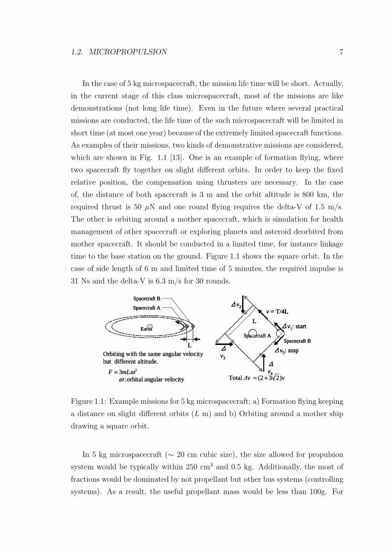
1.1 Example missions for 5 kg microspacecraft; a) Formation flying
keeping a distance on slight different orbits (L m) and b) Orbiting
around a mother ship drawing a square orbit. . . . . . . . . . . . . 7
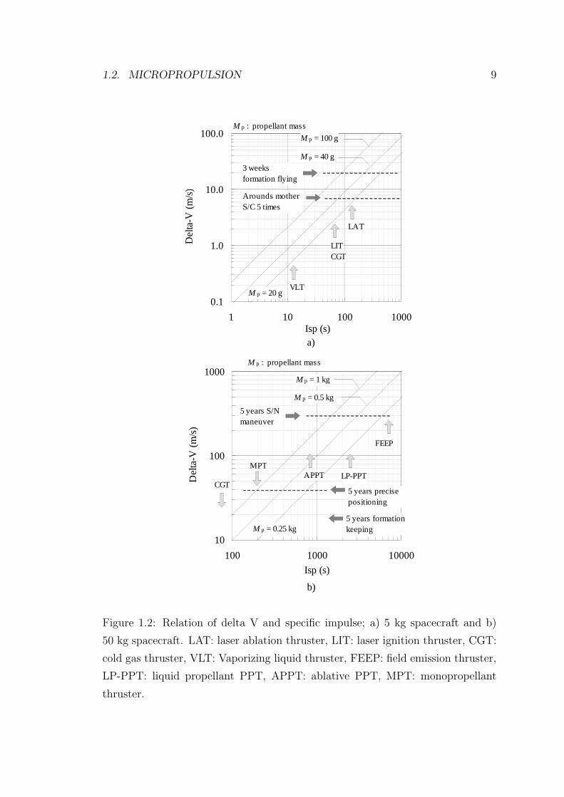
1.2 Relation of delta V and specific impulse; a) 5 kg spacecraft and b)
50 kg spacecraft. . . . . . . . . . . . . . . . . . . . . . . . . . . . . 9
2.1 Schematic drawing and photograph of the thrust stand system. . . . 25
2.2 Photograph of a flexural pivot with the rotational spring constant
of 0.191 Nm/rad. . . . . . . . . . . . . . . . . . . . . . . . . . . . . 27
2.3 Sample waveform of the oscillation of the balance with damping by
electrical feed lines (no magnetic damper). . . . . . . . . . . . . . . 28
2.4 Picture of the displacement sensor, LVDT: Linear Variable Differ-
ential Transformer, on the y − z stage. . . . . . . . . . . . . . . . . 29
2.5 Picture of the magnetic damper. . . . . . . . . . . . . . . . . . . . . 30
2.6 Magnetic damper feed back system. . . . . . . . . . . . . . . . . . . 31
2.7 Oscillation of the thrust stand by the thruster firing and its damping
using the electromagnetic damper. . . . . . . . . . . . . . . . . . . . 32
2.8 Picture of the linear stage and counter weights to control the gravity
center of the balance. . . . . . . . . . . . . . . . . . . . . . . . . . . 33
2.9 Limit cycle of counter weight adjustment. . . . . . . . . . . . . . . . 34
2.10 Sample of calibration; 20 sets of impulses measured by the force
transducer and the associated oscillation amplitude. . . . . . . . . . 36
2.11 Picture of the force transducer 209C01. . . . . . . . . . . . . . . . . 37
2.12 Picture of the impact pendulum to strike a force transducer. The
pendulum is manipulated by remotely controlling a propeller set on
a DC motor. . . . . . . . . . . . . . . . . . . . . . . . . . . . . . . . 38
xi
2.13 Sample of raw output of the force transducer. . . . . . . . . . . . . 39
2.14 Comparison of the oscillation amplitude with impulsive force and
short time force. . . . . . . . . . . . . . . . . . . . . . . . . . . . . . 42
2.15 Sample of the oscillation waveforms of the thrust stand by PPT
firing, capacitor-stored energy of a) 11.5 J and b) 2.9 J. . . . . . . . 44
2.16 Sample of the oscillation waveforms of the thrust stand by laser
ablation, the pulse width of a) 0.8 s and b) 0.2 s. . . . . . . . . . . 46
2.17 Comparison of the analysis methods. The relation of the ablated
mass and the impulse, a) result by the normal sinusoidal fitting and
b) result by the analysis method including the noise fitting curve. . 47
2.18 Picture of the thrust stand with additional springs and weights to
increase the stiffness of the balance. . . . . . . . . . . . . . . . . . . 48
2.19 Picture of the impact pendulum providing 100 mNs impulse. . . . . 50
2.20 Time history of the force transducer output striked by the huge
impulse pendulum (Fig. 2.19). . . . . . . . . . . . . . . . . . . . . . 52
2.21 Weighting functions according to fitting periods; [0, T0], [0, 2T0],
[−T0,−T0], [−2T0,−2T0], and [−3T0,−3T0]. . . . . . . . . . . . . . 55
2.22 Power spectrum density of the mechanical noise, calculated by FFT
from measured displacement of the balance. . . . . . . . . . . . . . 57
3.1 Conceptual diagram of the laser abaltion mode and laser ignition
mode. . . . . . . . . . . . . . . . . . . . . . . . . . . . . . . . . . . 62
3.2 Conceptual drawings of propellant feeding systems; a) tape-shaped
propellant and b) cylinder-shaped propellant. . . . . . . . . . . . . 64
3.3 Conceptual drawings of transmission modes for laser ablation and
ignition. . . . . . . . . . . . . . . . . . . . . . . . . . . . . . . . . . 66
3.4 Picture of the diode laser optical system: diode laser, collimation
tube, and focusing lens. . . . . . . . . . . . . . . . . . . . . . . . . . 69
3.5 Schematic diagram and dimensions of the diode laser optical system:
diode laser, collimation tube, and focusing lens. . . . . . . . . . . . 69
3.6 Drawing of typical diode laser beam. . . . . . . . . . . . . . . . . . 71
3.7 Beam profile at -2.0 mm from the focal point, a) 2D profile and b)
1D profile along the horizontal and vertical axis. . . . . . . . . . . . 72
xii
3.8 Beam profile at the focal point, a) 2D profile and b) 1D profile along
the horizontal and vertical axis. . . . . . . . . . . . . . . . . . . . . 72
3.9 Beam profile at +2.0 mm from the focal point, a) 2D profile and b)
1D profile along the horizontal and vertical axis. . . . . . . . . . . . 73
3.10 Profiles of beam widths along the beam axis. The solid and dashed
lines are fitted hyperbolic curves for vertical and horizontal axis
respectively. . . . . . . . . . . . . . . . . . . . . . . . . . . . . . . . 74
3.11 Laser beam intensity claculated from the beam width profiles. . . . 75
3.12 Configuration diagram of the laser beam and propellant. . . . . . . 76
3.13 Picture of the experiment setup used for both laser ablation and
laser ignition mode (the propellant in the picture is B/KNO3 py-
rotechnics of laser ignition mode). . . . . . . . . . . . . . . . . . . . 77
3.14 Thrust performance of laser ablation mode using commercially avail-
able black PVC sheet as propellant; a) generated impulse and ab-
lated mass and b) specific impulse and momentum coupling coefficient. 80
3.15 Picture of the PVC cylinders with different doped carbon density:
0, 2.5, and 5.0 %. . . . . . . . . . . . . . . . . . . . . . . . . . . . . 81
3.16 Thrust performance of laser ablation mode using custom-made PVCs
with carbon additives of 2.5 % and 5.0 %, a) generated impulse and
ablated mass and b) specific impulse and momentum coupling co-
efficient. . . . . . . . . . . . . . . . . . . . . . . . . . . . . . . . . . 82
3.17 Schematic diagram of plume direction measurement a) configura-
tion drawing and b) top view and definition of terms. . . . . . . . . 85
3.18 Scanned images contaminated by the exhaust gas: a) forward target
and b) bottom target. . . . . . . . . . . . . . . . . . . . . . . . . . 86
3.19 Deviation angle of thrust vector from the normal to the ablation
surface. . . . . . . . . . . . . . . . . . . . . . . . . . . . . . . . . . 87
3.20 Effect ot the multiple shots at the same point. . . . . . . . . . . . . 88
3.21 Mass spectrum during the repulsive operation in the laser ablation
mode: a) 1-100 amu and b) 32-42 amu. . . . . . . . . . . . . . . . . 90
3.22 Dehydrochlorination of PVC with subsequent formation of conju-
gated double bonds. . . . . . . . . . . . . . . . . . . . . . . . . . . . 91
3.23 Heating of solid by absorption of laser radiation. . . . . . . . . . . . 94
3.24 Numerically obtained plot of D∗(A). . . . . . . . . . . . . . . . . . 95
xiii
3.25 Approximation of a deviation factor from the surface heat flux ap-
proximation. . . . . . . . . . . . . . . . . . . . . . . . . . . . . . . . 97
3.26 Pre-sheath heat conduction. . . . . . . . . . . . . . . . . . . . . . . 98
3.27 Shift of temperature profile during stationary ablation. . . . . . . . 99
3.28 Relation of tge target position and ablated mass. . . . . . . . . . . 101
3.29 Relation of the laser intensity and ablated mass. . . . . . . . . . . . 102
3.30 Pictures of the pyrotechnics: composite propellant, double-base
propellant, and pelleted boron/potassium niterate (B/KNO3). . . . 103
3.31 Laser irradiation of composite propellant; a) Laser ignited com-
bustion in the atmosphere and b) no self-sustained combustion in
vacuum. . . . . . . . . . . . . . . . . . . . . . . . . . . . . . . . . . 104
3.32 Laser ignited combustion of B/KNO3 in vacuum. . . . . . . . . . . 105
3.33 Laser ignition probability of B/KNO3 in vacuum, dependence on
the laser pulse width. . . . . . . . . . . . . . . . . . . . . . . . . . . 107
3.34 Picture of the experiment setup for measuring the ignition probability.108
3.35 Laser ignition probability of B/KNO3 in vacuum, dependence on
the laser power. . . . . . . . . . . . . . . . . . . . . . . . . . . . . . 108
3.36 Conceptual diagram of a dual propulsive modes microthruster. . . . 110
3.37 Schematic diagrams of a one Newton class laser microthruster, a)
cross section of the single combustion chamber and b) a single prpel-
lant cartridge. . . . . . . . . . . . . . . . . . . . . . . . . . . . . . . 111
3.38 Picture a) and dimension b) of the one Newton class laser mi-
crothruster. . . . . . . . . . . . . . . . . . . . . . . . . . . . . . . . 112
3.39 Combustion plume of the one Newton class laser microthruster. . . 113
3.40 Impulse generaed by the one Newton class laser microthruster, using
two materials for the cartridge bodies. . . . . . . . . . . . . . . . . 114
3.41 Thermal feed back mechanism of typical solid propellant combustion.115
3.42 Conceptual drawings of a) three dimensional heating and b) heating
under spherical symmetry. . . . . . . . . . . . . . . . . . . . . . . . 119
3.43 Claculation grid and domain. . . . . . . . . . . . . . . . . . . . . . 121
3.44 Descretization on boudary. . . . . . . . . . . . . . . . . . . . . . . . 122
xiv
3.45 Calculated maximum temperature of B/KNO3 pyrotechnic after
one second laser heating, obtained by numerical simulation with
no exothermic reaction. The laser width along the horizontal axis
is 600 µm. . . . . . . . . . . . . . . . . . . . . . . . . . . . . . . . . 123
3.46 Schematic drawing of temperature profile in a combusting pyrotech-
nic. . . . . . . . . . . . . . . . . . . . . . . . . . . . . . . . . . . . . 125
3.47 Calculated temperature profiles on y = 0 plane with changing the
power and reaction rate. Three results are shown: no reaction,
quenching, and self-sustained combustion. . . . . . . . . . . . . . . 128
3.48 Mapping of the calculated result: ignition, quench, or no-reaction,
a)Wy =50 µm and b)Wy =110 µm. . . . . . . . . . . . . . . . . . . 129
3.49 Claculated threshold power for the laser ignition of B/KNO3 py-
rotechnic, a)k =1.6 W/mK and b)k =1.2 W/mK. . . . . . . . . . . 131
3.50 Claculated ignition time when 55 % of volume starts the reaction
(k =1.6 W/mK), a)Wy =50 µm and b)Wy =110 µm. . . . . . . . . 133
4.1 Conceptual drawing of an ablative PPT. . . . . . . . . . . . . . . . 136
4.2 Conceptual drawing of a liquid propellant PPT. . . . . . . . . . . . 138
4.3 Coordinate used in the formulation of electromagnetic acceleration. 140
4.4 Piezoelectric injector: a) schematic drawing and b) picture of the
operation in the atmosphere. . . . . . . . . . . . . . . . . . . . . . . 144
4.5 Schematic diagram of operation of a valve injector. . . . . . . . . . 145
4.6 Picture of the liquid injector used in this study. . . . . . . . . . . . 146
4.7 Pictures of water droplets ejected from the injector orifice, sequen-
tially taken every one millisecond. a) orifice diameter:50 µm and b)
orifice diameter: 25 µm. . . . . . . . . . . . . . . . . . . . . . . . . 147
4.8 Schematig diagram of the liquid PPT used here; a) materials and
b) dimensions. . . . . . . . . . . . . . . . . . . . . . . . . . . . . . . 148
4.9 Schematic diagram of the ablative PPT used here. . . . . . . . . . . 149
4.10 Pictures of the thrusters: a) LP-PPT and b) APPT. . . . . . . . . . 150
4.11 Schematic diagram of the spark plug. . . . . . . . . . . . . . . . . . 151
4.12 Pictures of the Rogowski coils: a) Type1 and b) Type2. . . . . . . . 152
4.13 Electrical connections assoiated with a Rogowski coil. . . . . . . . . 153
xv
4.14 Picture of the calibration setup using the current monitor. Copper
plate shorts the circuit in the atmosphere. . . . . . . . . . . . . . . 154
4.15 Typical waveforms of the calibration of the Rogowski coil. . . . . . 155
4.16 Electrical connections of power supplys and PPTs. . . . . . . . . . . 156
4.17 Typical discharge current waveform during the firing of the LP-PPT
at 11.5 J. . . . . . . . . . . . . . . . . . . . . . . . . . . . . . . . . 159
4.18 Measurement of the arc spark resistance between the anode and
copper plate. . . . . . . . . . . . . . . . . . . . . . . . . . . . . . . 160
4.19 Typical waveforms of voltage difference, current, and fitting-curve
of the voltage. . . . . . . . . . . . . . . . . . . . . . . . . . . . . . . 161
4.20 Resistance of the arc spark at the gap between the anode and copper
plate in the atomosphere. . . . . . . . . . . . . . . . . . . . . . . . . 161
4.21 Changing the position of the copper plate to measure the inductance
per unit length. . . . . . . . . . . . . . . . . . . . . . . . . . . . . . 162
4.22 Dependence of the inductance on the shorting position. . . . . . . . 163
4.23 Impulse bit dependence on the mass shot in the LP-PPT at 10.0 J
(2.6 kV). . . . . . . . . . . . . . . . . . . . . . . . . . . . . . . . . . 165
4.24 Specific impulse dependence on the mass shot in the LP-PPT at
10.0 J (2.6 kV). . . . . . . . . . . . . . . . . . . . . . . . . . . . . . 165
4.25 Impulse bit dependence on the capacitor stored energy in the LP-
PPT with interelectrode space of 20 and 40 mm. . . . . . . . . . . . 167
4.26 Total resistance dependence on the capacitor stored energy in the
LP-PPT with interelectrode space of 20 and 40 mm. . . . . . . . . . 167
4.27 Comparison of the impulse bit dependence on the energy between
the LP-PPT and APPT. . . . . . . . . . . . . . . . . . . . . . . . . 168
4.28 Comparison of the total resistance dependence on the energy be-
tween the LP-PPT and APPT. . . . . . . . . . . . . . . . . . . . . 168
4.29 Comparison of the specific impulse dependence on the energy be-
tween the LP-PPT and APPT. . . . . . . . . . . . . . . . . . . . . 169
4.30 Configuration of plasma observation system using a ultra high speed
camera. . . . . . . . . . . . . . . . . . . . . . . . . . . . . . . . . . 170
4.31 Successive images of plasma discharge of LP-PPT at the capacitor
stored energy of 10 J. . . . . . . . . . . . . . . . . . . . . . . . . . . 172
xvi
4.32 Successive images of plasma discharge of APPT at the capacitor
stored energy of 7.4 J. . . . . . . . . . . . . . . . . . . . . . . . . . 173
4.33 Emission intesnsity profile along the electrode. . . . . . . . . . . . . 175
4.34 Time history of the average position of the plasma emission. . . . . 176
4.35 Emission spectgrum during the LP-PPT firing with solute mixing
liquid; a) NaCl seeding and b) NH3 seeding. . . . . . . . . . . . . . 180
4.36 Thrust to power ratio dependence on the capacitor stored energy. . 181
4.37 Total resistance dependence on the capacitor stored energy. . . . . . 181
4.38 Dependence of vapor pressure of water on temperature. . . . . . . . 184
4.39 Microheater assembly. a) schematic drawing of a microheater as-
sembly and b) photograph before the gluing. . . . . . . . . . . . . . 186
4.40 Schematic diagrams of the LP-PPT using the microheater. . . . . . 188
4.41 Ignition probability dependence on the heater temperature. . . . . . 190
4.42 Pictures during the firing of LP-PPT using microheater; a) and
b): single discharge LP-PPT with close and open diaphragm of the
camera and c) and d) double discharge LP-PPT with close and open
diaphragm respectively (only c) with back ground light). . . . . . . 191
4.43 Thrust to power ratio dependence on the capacitor stored energy
in LP-PPT using microheater. . . . . . . . . . . . . . . . . . . . . . 193
4.44 Total resistance depdendence the capacitor stored energy in double
discharge LP-PPT using microheater. . . . . . . . . . . . . . . . . . 193
4.45 Comparison of the thrust to power ratio of Teflon PPT, spark plug
LP-PPT (pure water), and double discharge LP-PPT(the orifice of
D25 and D50 µm). . . . . . . . . . . . . . . . . . . . . . . . . . . . 195
4.46 Comparison of the total resistances of Teflon PPT, spark plug LP-
PPT (pure water), and double discharge LP-PPT(the orifice of D25
and D50 µm). . . . . . . . . . . . . . . . . . . . . . . . . . . . . . . 195
4.47 Dawgstar APPT desinged in University of Washington. . . . . . . . 197
A.1 Pulse response of a piezo force transducer. . . . . . . . . . . . . . . 217
A.2 Measured output voltage of the force transducer and its modified
output according to Eq. A.9. . . . . . . . . . . . . . . . . . . . . . . 219
B.1 Picture of UT space chamber. . . . . . . . . . . . . . . . . . . . . . 221
B.2 Schematic diagram of the evacuating system of UT space chamber. 222
xvii
B.3 Picture of TMAE cubic space chamber. . . . . . . . . . . . . . . . . 224
B.4 Schematic diagram of the evacuating system of TMAE space chamber.224
D.1 Thermal conductivity of boron-mixed-KNO3, temperature depen-
dence . . . . . . . . . . . . . . . . . . . . . . . . . . . . . . . . . . . 229
D.2 Thermal conductivity of boron-mixed-KNO3, dependence on the
volume fraction of boron at 400 K. . . . . . . . . . . . . . . . . . . 230
D.3 Thermal conductivity of boron-mixed-KNO3, dependence on the
volume fraction of boron at 700 K. . . . . . . . . . . . . . . . . . . 230
E.1 Conceptual drawing of a Rogowski coil. . . . . . . . . . . . . . . . . 231
E.2 RC integration circuit. . . . . . . . . . . . . . . . . . . . . . . . . . 233
E.3 Effect of the self inductance of a Rogowski coil on the output of the
RC integration circuit. . . . . . . . . . . . . . . . . . . . . . . . . . 235
F.1 LVDT signal conditioner. . . . . . . . . . . . . . . . . . . . . . . . . 238
F.2 Electromagnetic damper circuit. . . . . . . . . . . . . . . . . . . . . 239
F.3 Power supply of the piezoelectric force transducer. . . . . . . . . . . 240
F.4 Driving circuit of the liquid injector. . . . . . . . . . . . . . . . . . 240
F.5 High voltage pulse generator for the spark plug. . . . . . . . . . . . 241
F.6 Photo amplifier to generate TTL signal. . . . . . . . . . . . . . . . 241
F.7 Thermocouple conditioner. . . . . . . . . . . . . . . . . . . . . . . . 242
F.8 Temperature set-point controller. . . . . . . . . . . . . . . . . . . . 243
xviii
Chapter 1
Introduction
1.1 Microspacecraft
Microspacecraft have increasingly attracted the interest of researchers in recent
years[1]. Here microspacecraft mean miniaturized spacecraft down to less than 100
kg. In the early days of space exploration, the spacecraft were very light, Sputnik
weighed a little over 83 kg. It was because of the restrictions by a launcher. Sub-
sequent tremendous growth of technologies on aeronautics and astronautics made
it possible to increase the mass and size of spacecraft to acquire higher functions,
and the development had been directed toward highly functional, larger spacecraft.
However, these days the direction has started toward the miniaturization.
The miniaturization of spacecraft is motivated by the need to reduce in the cost
of developing and launching spacecraft. Up to date, space exploration had been
mainly conducted by government agencies in the world. Enormous cost associated
with the space exploration had prevented industry from the development, whereas
the importantness of the space is increasingly recognized. The expensiveness is
caused by developing and launching spacecraft. Spacecraft are constructed using
specially made components with extremely high reliability and durability. The
miniaturization will reduce the cost and also reduce the developing cycle, which
accelerates the growth of space development. Moreover, the most saving by the
microspacecraft will be the launch cost due to the mass and size reduction. For
instance, piggyback launch dramatically decreases the hurdle to launch spacecraft
for university and industry. Indeed, several universities have succeeded to launch
1
2 CHAPTER 1. INTRODUCTION
their microspacecraft in a last decade [2, 3, 4, 5].
The miniaturization improves in the mission capability, flexibility, and redun-
dancy using microspacecraft constellations. Partitioning the functions of a single,
large, highly functional spacecraft into a number of smaller spacecraft has a lot of
potentials. Cluster of spacecraft cooperatively conduct missions with orbiting in
close each other. Changing the role of each spacecraft according to the situation
increases the probability of success for the mission. A trouble on one spacecraft
would not affect the other spacecraft and that role is covered by the others. The
increasing redundancy also enables to construct spacecraft using ordinary avail-
able components, which causes the reducing cost again. Moreover such cluster
or platoon of microspacecraft enables advanced missions that otherwise could not
be performed. Several studies using the formation flying are studied [6, 7, 8, 9].
Terrestrial Planet Finder (TPF) [10] by National Aeronautics and Space Admin-
istration (NASA) and Darwin[11] by European Space Agency (ESA) are missions
to search Earth-like planets outside the solar system. They use multiple spacecraft
with telescopes as a large telescope with a diameter of several 100 meters using
interferometric imaging, which provide high sensitivity and resolution. Laser In-
terferometery Space Antenna (LISA) [12] (joint mission by NASA and ESA) is a
space-based gravitational wave observatory using laser interferometry with large
distance. Although such advanced missions are not to use microspacecraft (they
are over 100 kg), the technologies can be applied to microspacecraft and increase
the variety of microspacecraft missions.
In addition to the formation flying, microspacecraft is expected to perform
health management of the mother spacecraft or to probe planets and asteroid in
deep space exploration. Microspacecraft could not have the capability to orbit
far away from the earth by themselves. However they can be carried on a large
spacecraft because of their small size, and deorbited in deep space to conduct such
various missions.
1.2. MICROPROPULSION 3
1.2 Micropropulsion
1.2.1 Role of micropropulsion
A key element for microspacecraft operations is a practical micropropulsion sys-
tem. These days microspacecraft have been studied, developed, and launched by
government agency, industry, and universities. However, their missions remain in
the state of the demonstration for microspacecraft. Strictly limited weight and
size for the microspacecraft leads to various constrictions for spacecraft hardware.
Especially the lack of propulsion systems reduces the variety of missions. Attitude
control of spacecraft is attainable by passive systems such as momentum wheels
and magnetic torqueres. Actually, state-of-the-art microspacecraft perform their
attitude control using such systems as minimum as possible (whereas unloading of
the momentum wheel requires propulsion). In contrast, translation motion of the
spacecraft inevitably requires propulsive capability. Advantages of microspacecraft
will be developed conducting cooperrative works by the constellation or orbiting
by themselves, which essentially need translation motion. Therefore in order to
enable advanced microspacecraft missions, a small propulsion system suitable for
microspacecraft, namely a microthruster, is needed.
Microspacecraft dealt in this study have the weight ranging from 1 to 100 kg.
That class spacecraft is categorized into class I/II microspacecraft by NASA and
Micro/Nano spacecraft by AFRL. The corresponding spacecraft’s dimension and
power are 0.1 to 1 m and 1 to 100 W. State-of-the-art propulsion hardware can be
applicable to more than 100 kg spacecraft in most cases. Hence, newly developed
technology is required to accomplish such small miniaturized spacecraft.
1.2.2 Problems to the miniaturization
Micropropulsion systems must be designed to overcome a number of challenges
associated with the miniaturization. The difficulties of micropropulsion system
are manufacturing and integrating complexity, degenerating efficiency according
to the scaling low, propellant leakage and clogging, contamination problems from
the plume, and limited power for electric propulsions. Which factor affects most
4 CHAPTER 1. INTRODUCTION
depends on the variety of the thruster. The manufacturing and integrating com-
plexity is included in all thrusters. The complexity mainly comes from the pro-
pellant feeding system, pressurizing or mixing the propellant, and plasma con-
finement. Some researchers expect MEMS as a key technology to solve those
problems. However, state-of-the-art MEMS technology has not reached to the
level for practical applications. Decreasing the scale leads to several inefficiency
because of increased boundary layer, heating loss, and plasma loss. Concerns of
the propellant leakage and clogging are associated with microspacecraft unless us-
ing solid phase propellant. With the scaling down, leakage rate of the propellant
will remain in the same level, or may be worse. Hence the percentage of the leak-
age in the total propellant mass becomes larger with decreasing the size. Also
miniaturization will increase the probability of clogging, which often becomes a
cause of the failure of propulsion system. Contamination becomes concern for
spacecraft system, degenerating the solar cell, as well as usual spacecraft. The
miniaturization consequently leads to less power, and it increases the difficulty
using electric propulsion. A lot of electric propulsion work most effectively using
power more than a few 100 W.
1.2.3 Required propulsive capabilities
Requirements for thrust level
The propulsive capabilities required for micropropulsion will be widely varied ac-
cording to the mission and size of the spacecraft. The requirement is roughly said
as the lower range thrust and the higher range thrust. In the case of attitude
control, lower thrust is required for precise positioning and higher thrust is for
slew maneuvers. In the case of formation flying, they need lower thrust for the
constellation controls and higher thrust for the re-arrangement of their formation
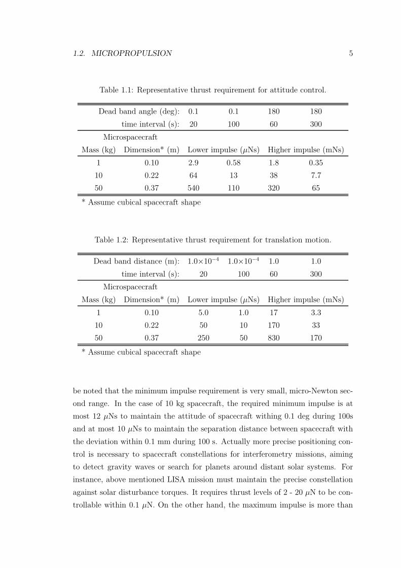
patterns. Tables 1.1 and 1.2 summarize representative thrusts required for the at-
titude control and translation motion of microspacecraft. Those thrusts (impulses)
were evaluated assuming several dead bands and time interval between thrust fir-
ings, where dead band is angle or distance by which spacecraft moves during the
time interval, namely resolutions for spacecraft control. In the case of the evalu-
ation of attitude control, cubical spacecraft shape was assumed, and the typical
dimension and impulse were calculated based on the spacecraft mass. It should
1.2. MICROPROPULSION 5
Table 1.1: Representative thrust requirement for attitude control.
Dead band angle (deg): 0.1 0.1 180 180
time interval (s): 20 100 60 300
Microspacecraft
Mass (kg) Dimension* (m) Lower impulse (µNs) Higher impulse (mNs)
1 0.10 2.9 0.58 1.8 0.35
10 0.22 64 13 38 7.7
50 0.37 540 110 320 65
* Assume cubical spacecraft shape
Table 1.2: Representative thrust requirement for translation motion.
Dead band distance (m): 1.0×10⁻⁴ 1.0×10⁻⁴ 1.0 1.0
time interval (s): 20 100 60 300
Microspacecraft
Mass (kg) Dimension* (m) Lower impulse (µNs) Higher impulse (mNs)
1 0.10 5.0 1.0 17 3.3
10 0.22 50 10 170 33
50 0.37 250 50 830 170
* Assume cubical spacecraft shape
be noted that the minimum impulse requirement is very small, micro-Newton sec-
ond range. In the case of 10 kg spacecraft, the required minimum impulse is at
most 12 µNs to maintain the attitude of spacecraft withing 0.1 deg during 100s
and at most 10 µNs to maintain the separation distance between spacecraft with
the deviation within 0.1 mm during 100 s. Actually more precise positioning con-
trol is necessary to spacecraft constellations for interferometry missions, aiming
to detect gravity waves or search for planets around distant solar systems. For
instance, above mentioned LISA mission must maintain the precise constellation
against solar disturbance torques. It requires thrust levels of 2 - 20 µN to be con-
trollable within 0.1 µN. On the other hand, the maximum impulse is more than
6 CHAPTER 1. INTRODUCTION
mili-Newton second range. In the case of 10 kg spacecraft, the required impulse is
38 mNs to rotate the spacecraft in the opposite direction in 1 min and 170 mNs to
translate the spacecraft with the velocity of 1 m/min. Such huge impulse would
not be accomplished without certain micro-chemical propulsion.
The most important for state-of-the-art microspacecraft is the further minia-
turization to expand the varieties of missions. Therefore, the requirement for mi-
cropropulsion is in first the ability to be installed on such microspacecraft rather
than their performance. Additionally their missions are like demonstrations and
the life times are relatively shorter than commercially available spacecraft. There-
fore large delta-v is not required. However, in the next stage, highly functional mi-
crospacecraft would be required, and long mission time, hence large delta-V, will
be necessary. In such advanced long-term missions, micropropulsion with high
specific impulse becomes very attractive. The propellant tank must be eventu-
ally miniaturized, because of the high percentage of spacecraft mass and volume.
Moreover, future challenging missions would require microspacecraft proceed in
deep space by themselves using primary micropropulsion system. Small-body ren-
dezvous and outer planet orbiters have substantially higher delta-v requirements.
In those large delta-V missions, micro-electric propulsion system become neces-
sary.
Micropropulsion is used for not only microspacecraft but also large spacecraft
to control and restrain the deformation of the huge structure. In the stream of
increasing the size and function of spacecraft, spacecraft have increasingly required
larger power, which is accomplished enormous solar cell. Such enormous solar cell
will be expanded in the space and the deformation should be prevented. Several
micropropulsion system would be suitable to help expanding the cell and keep the
formation due to their compactness.
Requirements for delta-V
Next, propulsive capability for microspacecraft is discussed in terms of delta-V.
It is strongly related to the life time of spacecraft and specific impulse of the
propulsion system. The requirement will be widely changed according to the
mission as well as the thrust requirement. Here, only a few representative missions
are considered as the examples for 5 kg and 50 kg microspacecraft missions.
1.2. MICROPROPULSION 7
In the case of 5 kg microspacecraft, the mission life time will be short. Actually,
in the current stage of this class microspacecraft, most of the missions are like
demonstrations (not long life time). Even in the future where several practical
missions are conducted, the life time of the such microspacecraft will be limited in
short time (at most one year) because of the extremely limited spacecraft functions.
As examples of their missions, two kinds of demonstrative missions are considered,
which are shown in Fig. 1.1 [13]. One is an example of formation flying, where
two spacecraft fly together on slight different orbits. In order to keep the fixed
relative position, the compensation using thrusters are necessary. In the case
of, the distance of both spacecraft is 3 m and the orbit altitude is 800 km, the
required thrust is 50 µN and one round flying requires the delta-V of 1.5 m/s.
The other is orbiting around a mother spacecraft, which is simulation for health
management of other spacecraft or exploring planets and asteroid deorbited from
mother spacecraft. It should be conducted in a limited time, for instance linkage
time to the base station on the ground. Figure 1.1 shows the square orbit. In the
case of side length of 6 m and limited time of 5 minutes, the required impulse is
31 Ns and the delta-V is 6.3 m/s for 30 rounds.
L
Spacecraft A
Spacecraft B
Earth
Orbiting with the same angular velocitybut different altitude.
Δv5: stop
Δv1: start
Δv2
Δ
v3
Δ
v4
Spacecraft ASpacecraft B
L
v = T/4L
v∆v )232( Total +=23 ωmLF =
locityangular ve orbital :ω
L
Spacecraft A
Spacecraft B
Earth
L
Spacecraft A
Spacecraft B
Earth
Orbiting with the same angular velocitybut different altitude.
Δv5: stop
Δv1: start
Δv2
Δ
v3
Δ
v4
Spacecraft ASpacecraft B
L
v = T/4L
Δv5: stop
Δv1: start
Δv2
Δ
v3
Δ
v4
Spacecraft ASpacecraft B
L
v = T/4L
v∆v )232( Total +=23 ωmLF =
locityangular ve orbital :ω
Figure 1.1: Example missions for 5 kg microspacecraft; a) Formation flying keeping
a distance on slight different orbits (L m) and b) Orbiting around a mother ship
drawing a square orbit.
In 5 kg microspacecraft (∼ 20 cm cubic size), the size allowed for propulsion
system would be typically within 250 cm3 and 0.5 kg. Additionally, the most of
fractions would be dominated by not propellant but other bus systems (controlling
systems). As a result, the useful propellant mass would be less than 100g. For
8 CHAPTER 1. INTRODUCTION
instance, in the case of a cold gas thruster with xenon gas, 100 cm3 would be used
for high pressure (100 atm) gas tank and the propellant mass would be about 40
g. The other space must be used for pressure regulator, valves, nozzle, and so
on. In the case of a laser ignition thruster, which is addressed in this study (see
Chapter 3), five solid propellant cartridges would be allowed and the mass of solid
propellant is also 40 g. The other space must be used for laser diode driver and
propellant feeding system.
Figure 1.2 shows the relation of specific impulse and acquired delta-V for 5 kg
spacecraft. Within the limit of propellant mass (20, 40, 100 g cases are shown in the
figure), at least Isp of 50 s is necessary to conduct above-mentioned microspacecraft
missions. Therefore, low Isp thruster like a vaporizing liquid thruster would not
be adequate for this class mission, unless bringing a lot of propellant mass. Laser
ablation thruster, also addressed in this study, with low thrust but high Isp of
100-150 s would be suited for keeping formation flying and laser ignition thruster
with high thrust but low Isp will be suited for the maneuver in very short time.
In the case of 50 kg microspacecraft (∼ 40 cm cubic size), the size allowed
for propulsion system would be typically within 2500 cm3 and 5 kg. There the
missions would be close to those of conventional highly functional spacecraft with
more than a few years of the life time for practical use. For instance, let us
consider North-South maneuver in GEO (geostationary orbit) which is the most
practical orbit for spacecraft. Large, highly functional spacecraft currently used
in GEO can be replaced by constellation of microspacecraft to increase the system
redundancy. Of course these microspacecraft should be brought by other large
spacecraft or transfer rocket supplying high delta-V because transfer from LEO
(low earth orbit) to GEO requires huge delta-V about 4 km/s.
In GEO most important propulsion task would be North-South maneuver. It is
compensation of the orbit inclination due to the several disturbances on the orbit.
The most causes are gravitations from the sun and moon. Both accelerations are
8.6×10⁻⁶ and 3.4×10⁻⁶ m/s2 by the moon and sun respectively. As a result, the
required delta-V for the N/S maneuver for one year is usually about 50 m/s[14].
Solar pressure is another disturbance forces for spacecraft, which is about
4.5×10⁻⁶ N/m2 near the earth. In the case of 40 cm cubic microspacecraft, the
applied force is 7×10⁻⁷ N and much smaller than the gravitational disturbances.
Also, the atmospheric drag is much smaller than solar pressure in GEO.
1.2. MICROPROPULSION 9
0.1
1.0
10.0
100.0
1 10 100 1000Isp (s)
Del
ta-V
(m
/s)
M p = 100 g
M p = 40 g
M p = 20 g
3 weeksformation flying
Arounds motherS/C 5 times
CGTLIT
VLT
LAT
M p : propellant mass
10
100
1000
100 1000 10000
Isp (s)
Del
ta-V
(m
/s)
M p = 1 kg
M p = 0.5 kg
M p = 0.25 kg
5 years S/Nmaneuver
APPT LP-PPT
FEEP
CGT5 years precisepositioning
MPT
5 years formationkeeping
M p : propellant mass
a)
b)
Figure 1.2: Relation of delta V and specific impulse; a) 5 kg spacecraft and b)
50 kg spacecraft. LAT: laser ablation thruster, LIT: laser ignition thruster, CGT:
cold gas thruster, VLT: Vaporizing liquid thruster, FEEP: field emission thruster,
LP-PPT: liquid propellant PPT, APPT: ablative PPT, MPT: monopropellant
thruster.
10 CHAPTER 1. INTRODUCTION
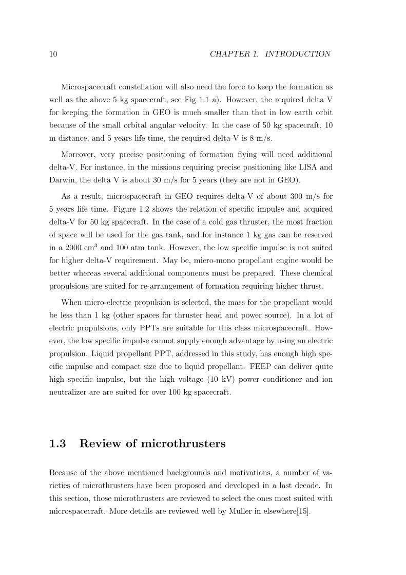
Microspacecraft constellation will also need the force to keep the formation as
well as the above 5 kg spacecraft, see Fig 1.1 a). However, the required delta V
for keeping the formation in GEO is much smaller than that in low earth orbit
because of the small orbital angular velocity. In the case of 50 kg spacecraft, 10
m distance, and 5 years life time, the required delta-V is 8 m/s.
Moreover, very precise positioning of formation flying will need additional
delta-V. For instance, in the missions requiring precise positioning like LISA and
Darwin, the delta V is about 30 m/s for 5 years (they are not in GEO).
As a result, microspacecraft in GEO requires delta-V of about 300 m/s for
5 years life time. Figure 1.2 shows the relation of specific impulse and acquired
delta-V for 50 kg spacecraft. In the case of a cold gas thruster, the most fraction
of space will be used for the gas tank, and for instance 1 kg gas can be reserved
in a 2000 cm3 and 100 atm tank. However, the low specific impulse is not suited
for higher delta-V requirement. May be, micro-mono propellant engine would be
better whereas several additional components must be prepared. These chemical
propulsions are suited for re-arrangement of formation requiring higher thrust.
When micro-electric propulsion is selected, the mass for the propellant would
be less than 1 kg (other spaces for thruster head and power source). In a lot of
electric propulsions, only PPTs are suitable for this class microspacecraft. How-
ever, the low specific impulse cannot supply enough advantage by using an electric
propulsion. Liquid propellant PPT, addressed in this study, has enough high spe-
cific impulse and compact size due to liquid propellant. FEEP can deliver quite
high specific impulse, but the high voltage (10 kV) power conditioner and ion
neutralizer are are suited for over 100 kg spacecraft.
1.3 Review of microthrusters
Because of the above mentioned backgrounds and motivations, a number of va-
rieties of microthrusters have been proposed and developed in a last decade. In
this section, those microthrusters are reviewed to select the ones most suited with
microspacecraft. More details are reviewed well by Muller in elsewhere[15].
1.3. REVIEW OF MICROTHRUSTERS 11
1.3.1 Micro-chemical propulsion
Up to date almost all propulsion systems used for the space exploration are chemi-
cal propulsions due to their simpler physics, and higher completeness, than electric
propulsion. The interests are focused on the developing and fabricating the com-
mercial products rather than the fundamental research. Therefore they are con-
ducted mainly by government agency and industry. However, the miniaturization
of those propulsion includes a number of unknown problems and characteristics,
and many researchers in universities have started the studies.
In comparison with electric propulsion, chemical propulsion is characterized by
the higher thrust and no need of an electrical power source. Therefore, it would
be suitable with extremely small and short life time microspacecraft.
Cold gas thruster
Cold gas thrusters simply exhaust gas with no chemical reaction from a pressurized
propellant tank. In the tank, the propellant is stored with 1 to 200 atms. Hence
the specific impulse is small, usually ranged from 30 to 100 s, unless very light gas
like H2 and He is used. Nitrogen is the most frequently used propellant, which
gives the specific impulse around 70 s.
The most advantage is the simplest structre in the other gas thrusters. It has
been miniaturized already over the other thrusters. Moreover, when using benign
gas, the cold gas thruster is relieved from spacecraft contamination problems.
Nevertheless, propellant leakage and clogging problems and heavy, high-pressure
propellant storage still remain as disadvantage. Use of ammonia as the propellant
is interesting and promising idea because it will enable the liquid storage and
reduce the tank size and mass.
Mono/Bi-propellant engines
Bipropellant engines are frequently considered for primary propulsion applications
on conventional spacecraft because of their high thrust and high specific impulse.
They mix two gaseous (fuel and oxidizer) and get high specific impulse, up to
300 s. Nitrogen tetroxide (NTO) and monomethylhedrazine (MMH) as oxidizer
and fuels are used in the most cases. However, its complexity using separate
feeding systems for fuel and oxidizer is disadvantage. Also leakage and clogging of
12 CHAPTER 1. INTRODUCTION
propellants becomes concern as well as or more than cold gas thrusters due to the
complex system. Moreover, combustion efficiency and mixing losses are affected
by the miniaturization, and the associated degradation of the performance would
be worse than cold gas thrusters.
Using power MEMS technology for micro-bipropellant engine have been pro-
posed and examined [16]. They accomplished the chamber pressure up to 12 atm
(over the pressure failed the motor) and got the 1 N thrust. The most problems of
such thrusters using power MEMS are suitable valve development, which should
be fabricated using MEMS. Several MEMS based thruster suffers from the lack of
suitable micro-valve.
Micro monopropellant engines are positioned between bipropellant engines and
cold gas thrusters in the specific impulse and complexity. Hence the advantages
and disadvantages are also middle of them. However, from the view point of the
contamination, they have worse than both thrusters. It is because that they use
most commonly hydrazine as monopropellant, which have high toxicity. It also
costs the ground test and propellant loading procedure.
Recently HAN-based monopropellant engines have attracted interests, which
uses a mixture of an oxygenrich component called HAN (hydroxylammonium ni-
trate) and a fuel-rich component. It is characterized by the non-toxicity.
Digital microthruster array
Solid rocket motors have advantages of the that compact size, no propellant feed-
ing system, high specific impulse. However, the obvious disadvantage is difficulty
to use arbitrary of quantity, that is they are not restartable. One of the methods to
solve the problem is partitioning solid propellant into small pellets and installing
them into a numbmer of micro chambers, whereas the installing micro-chamber
leads to decrease of the energy density. Several researchers have examined that
idea using power MEMS technology [17, 18, 19, 20], which are called as digital
microthruster or micro solid rocket array. Micro-chambers with the dimension of
1 mm or below are fabricated and arrayed on a single chip. Every micro solid
propellant is ignited by a heat element. Their solid rockets have very high energy
density, namely small propellant tank volume, and are released from the propellant
1.3. REVIEW OF MICROTHRUSTERS 13
feeding concerns. However, they suffer from low ignition probability and low com-
bustion efficiency. Inexact touching of heat element on the propellant caused the
failure of the ignition. Also another disadvantage is the change of the trust vector
by shot-to-shot. In the propulsive task of translation motion, the synchronous
firing of multiple propellants with symmetry at the center (thrust point) would
solve the problem to some extent.
1.3.2 Micro-electric propulsion
In contrast to long history of the practical use of the chemical propulsions, electric
propulsion has started to be applied in a last decade. The research on electric
propulsions started since the early days (1960s) [21, 22]. However, in the space
exploration which needs high reliability, they hardly changes already-established-
systems into novel systems, even if they are superior than old ones. In last decades,
several missions have started installing electric propulsions in challenging deep
space missions [23, 24, 25, 26, 27].
Micro-electric propulsion systems are characterized by the high specific impulse
over the micro-chemical propulsion. High specific impulse decreases the size and
weight of propellant tank, which had dominated the fraction in the size and mass of
spacecraft subsystems. On the other hand, electric propulsions are disadvantaged
by the need of a high voltage power source. Then the reduction of propellant tank
must be enough to compensate the increase of the power source.
The scaled-down of electric propulsion would lead to several inefficiency as well
as chemical propulsion. Increased surface to volume ratio by the miniaturization
increases the plasma losses to walls.
Pulsed Plasma Thruster
In electric propulsions, Pulsed Plasma Thrusters (PPTs) [28] have very simple
structures and robustness in comparison to others. They utilize solid polymer
Teflon r©(PTFE) as the propellant. The polymer surfaces which contacts to plasma
are ablated by the plasma and fed into it as propellant (discharge ablation feed-
ing). Such PPTs are sometimes called as ablative PPTs or ablation fed PPTs
(APPTs) to distinguish PPTs using gas or liquid as the propellant. The receded
propellant is re-fueled by simply pushing the back using a spring. Then they are
14 CHAPTER 1. INTRODUCTION
released from the complex propellant feeding system and concern of propellant
leakage. Moreover their capability to work with low energy (1 to 10 J) is suit-
able with power-limited microspacecraft. The thrust is generated in very short
time ( 5 µs), and that impulsive thrust enables digital control of the impulse with
high resolution. A dditionally, the thrust efficiency is independence on the firing
frequency, and the thrust can be arbitrarily throttled within the allowed electric
power.
On the other hand, associated problems with PPTs are their low thrust perfor-
mance and concern of contamination from the ablated gas. Most electric propul-
sions currently used for several missions have the thrust efficiency of 50 % and the
specific impulse of 1500 to over 3000 s. However typical flight qualified PPTs have
the performance of less than 10 % and 800 s. Many researchers have considered
that those poor performance comes from the excessive propellant feeding due to
discharge ablation. The ablated propellant is kept to be evaporated from the solid
surface even after the discharge termination.
Micro electrostatic thruster
Electrostatic propulsions, represented by ion engines and Hall thrusters, are lead-
ing thrusters in electric propulsions, and used in several missions as primary en-
gines [23, 24, 25, 26, 27]. Neutral particles are ionized into ions in a discharge
chamber and they are electrostatistically accelerated by voltage difference of 300
(Hall thruster) to 1000 (ion engine) V. The extracted ion beam is neutralized using
a neutralizer, where hollow cathodes are often used due to their low electron cost.
Xenon is frequently used as the propellant, because of the relative low ionization
potential of heavy and benign gaseous.
Their great achievement in several missions have attracted researchers’ inter-
est to apply them to micropropulsions. Then micro-ion-engine and micro-Hall-
thrusters have been proposed and developed [29, 30, 31, 32, 33]. However, the
scaled-down causes the performance decreasing. Electrostatic propulsions con-
fine plasma using magnetic field, where Larmor radius of the particles should be
less than the characteristic length. Hence the decreasing size of thrusters requires
stronger magnetic field to confine plasma. Even if enough magnetic field is applied,
the increased surface volume ratio leads to more plasma losses. Also decreased
1.3. REVIEW OF MICROTHRUSTERS 15
power causes the higher ion beam cost. In addition, the need of ion beam neutral-
izer leads to system complexity and make the miniaturization difficult.
Field emission thruster
Field emission electric propulsions (FEEPs) are also electrostatic thrusters but
with unique characteristic on the plasma generation processes [34, 35]. They
directly extract atomic ions from the free surface of liquid metal at the edge of an
emitter. The emitter has needle or slit shape and liquid metal is fed through or
wetted on it by the action of capillary forces. High voltage of 10 kV range is applied
at the edge and the strong electric field is generated. When the field reaches a
threshold value (106 V/mm), atoms on the liquid surface are eventually extracted
and electrostatistically accelerated. Cesium or indium are usually selected as the
propellant.
The FEEPs are characterized by their ultra high specific impulse of 4000-10000
s range because of the high applied voltage. Also they can deliver extremely
small thrust in the 1-10 µN range. It is suitable for accurate positioning of the
spacecraft. Their unique plasma generation method, with no discharge chamber,
inherently avoids the plasma losses into walls and leads to high efficiency (over 70
%). Moreover it removes the concern related to volume surface ratio and suitable
for the scaled-down.
The disadvantages of FEEPs are concerns on electromagnetic interaction (EMI)
due to their high voltage. Additionally use of high applied voltage requires heavier
power supply than lower voltage devices with the same power range. As well as
the other electrostatic thrusters, FEEP requires an neutralizer for the ion beam.
Colloid thruster
Colloid thrusters have similar acceleration mechanism as FEEPs and were stud-
ied in 1960s to 1970s proceeding in FEEPs [36, 37]. High voltage is applied to
a capillary tube with liquid propellant, and not atomic ions but charged liquid
droplets are extracted from the emitter. They use solutions as propellant, for in-
stance glycerol doped with sodium iodine to produce positive droplets and glycerol
doped with sulfuric to produce negative droplets. In the development of colloid
thrusters, specific charge, defined as charge per droplets mass, is a key factor to
16 CHAPTER 1. INTRODUCTION
determine the performance. The typical values are in the range of 102 to 105
Coul/kg. Recently, application of MEMS technology [38] and examinations of
alternative propellants [39, 40] are studied.
The using no discharge chamber gives the similar characteristics as FEEPs.
In comparison to FEEPs, colloid thrusters have higher thrust (200 µN/W) and
lower specific impulse (500 - 1500 s). In addition, unique ability to produce both
positive and negative droplets according to the solutes enables self-neutralizing
colloid thruster with bipolar array. It eliminates the disadvantage of needing a
neutralizer.
Micro Resisto/arc-jet thruster
resistojet or arcjet thrusters convert the electric energy into the thermal energy
using a resistive heater or arc discharge respectively, and electrothermally acceler-
ate the propellant. They provide higher thrust than other electric propulsions but
lower specific impulse around 200-500 s. Resist/arc-jets provide specific impulse as
well as bipropellant engine without the complexity of such engines. However they
requires an additional power source. Difficulty in the miniaturization is similar
to chemical propulsions, inefficiency of scaled-down and propellant leakage and
clogging. In recent years, a very low power arcjet (a few W) has been studied
[41, 42, 43].
Laser ablation microthruster
Laser ablation microthrusters are sometimes categorized into a beaming propulsion
rather than electric prpulsions. The beaming propulsion is to transmit the energy
from outside of the spacecraft using beam (as laser, microwave, or solar window)
[44, 45, 46]. It has the potential for significant weight reduction and improved the
payload ratio. The beaming propulsion can be categorized into several types, by
the laser types or the energy conversion processes. A laser ablative propulsion is
one of those [46, 47], which focuses and irradiates the laser beam on the surface of
a solid propellant (metals and polymers). The heated and evaporated propellant
by the laser beam is ejected from the surface (laser ablation) to provide thrust.
Phipps et al. proposed the use of laser diodes for the laser ablative propulsions
1.3. REVIEW OF MICROTHRUSTERS 17
as a micropropulsion [48, 49], as the miniaturization of spacecraft increasingly at-
tracted attentions, The thruster is referred as a diode laser ablation microthrusters
in this study. The propulsion system includes diode lasers, optical system, and
solid ablative propellant. The compactness of laser diodes and the associated op-
tical system enable an onboard laser beam source. Actually, typical diode lasers
weigh 1-2 g and less than 10 g even with the optical system. In addition to the
compactness, laser diodes have advantages of low operation voltage and high con-
vergent efficiency. Diode lasers require the operation voltage less than 5 V and
have the convergent efficiency over 40 %. Solid polymer is commonly used as the
propellant (ablative material) for the diode laser ablation microthruster, because
most diode lasers do not have enough intensity to ablate metals.
The diode laser ablation microthrusters are characterized by the compactness,
the use of solid propellant, and the accurate thrust control. The compactness of
diode lasers and the low operating voltage enable the higher miniaturization than
other electric propulsions. The use of solid propellant solves the problem of the
propellant leakage and clogging as well as PPTs. The thrust can be widely and
precisely adjusted by varying the laser pulse width.
In contrast, the disadvantages are their feeding system and lens fouling. They
must equip a certain mechanism to feed solid propellant for the laser irradiation.
The propellant feeding system should be compact, light weight, and long life time.
Developing such a feeding system is essential to realize the diode laser ablation mi-
crothruster. Lens fouling by the plume jet becomes severe problem for propulsions
using beaming energy. Phipps et al. have proposed and examined the transparent
mode ablation to defeat that problem, where laser beam irradiate the propellant
from the opposite direction to the plume jet through transparent material. How-
ever that mode decreased the thrust by half and limits the varieties of usable
propellant.
1.3.3 MEMS based propulsion
MEMS based propulsion systems allow extremely small devices to be applied to
microspacecraft less than 1 kg. Hence several MEMS-based thrusters have been
proposed; MEMS-based, cold gas thruster, resistojet, FEEP, and ion engine. It
will allow to integrate different propulsion components on a single MEMS chip,
18 CHAPTER 1. INTRODUCTION
saving the size and weight for thrusters. However many of these concepts are still
in the very early development stage. The most important component is a valve
controlling the propellant. The valve with low leakage rate and long life-time
should be developed to apply MEMS based propulsion to microspacecraft.
Additionally, excessive miaturization using MEMS would have less benefit. It
is because that the most dominate size and weight in propulsions is not a thruster
head but propellant and its feeding system. The minimum size allowed for a
thruster head would be determined by the propellant. Then the head should be
designed to provide as high efficiency as possible within the range. The excessive
miaturization would only increase disadvantages associated with the scaled-down.
1.4 Microthrusters for 1-100 kg microspacecraft
In this study, a diode laser microthruster with dual propulsive mode and pulsed
plasma thruster using liquid propellant are selected as promising micropropulsions
for 1-10 kg and 10-100 kg microspacecraft respectively.
1.4.1 Dual propulsive mode diode laser microthruster
The ability required for propulsion of 1-10 kg microspacecraft is first the compact-
ness rather than high specific impulse. The missions expected for such microspace-
craft would be commonly simple and short-time missions, because the function is
quite restricted due to severe limits of the size, weight, and power. The bus sys-
tem dominates most of the volume and weight, and only a small fraction would
be provided for sensing devices and propulsions. The electric power that such
microspacecraft provide for propulsion system is restricted at most a few Watts
in the current stage, at most 20 W even in the near future. Orbit raising needing
large delta-v or constellation controlling in long time, over a few years, are not
required (impractical) for this class spacecraft.
Therefore high specific impulse of electric propulsions are not so attractive
for that class microspacecraft. Additionally loading an additional power source
for propulsions would prevents them from the application in such small space-
craft. Chemical propulsions using gas propellant, cold gas thrusters and mono/bi-
propellant engines, are also not suitable due to their propellant feeding system.
1.4. MICROTHRUSTERS FOR 1-100 KG MICROSPACECRAFT 19
Those systems need strict, complex, and heavy components by handling and stor-
ing highly pressurized propellant. Moreover they gives several risks of propellant
leakage and clogging. MEMS-based microthrusters may have the most advantage
in the scale. However, their technologies are not in the practical stage. After
all digital microthruster array and laser ablation microthruster are suitable for
1-10 kg microspacecraft (whereas laser ablation microthrusters are categorized in
electric propulsions but they need a power source with only a few W).
The propulsion capable to generate both the lower range and higher range
thrust is very attractive for 1-10 kg microspacecraft. The applications of the
propulsion are represented by accurate constellation positioning and attitude con-
trol using lower thrust and re-arrangement of the constellation and slew manevver
using higher thrust. In order to limit the weight and size of the microspacecraft,
it is essential to satisfy the requirement of lower and higher range thrusts with
the same propulsion system. To our knowledge, there is as yet no single propul-
sion system which can supply such a wide range of thrust for the 1-10 kg class
microspacecraft.
In this study, a novel type of microthruster enabling multiple propulsive tasks
is proposed. That microthruster has dual propulsive modes using a diode laser:
laser ablation mode and laser ignition mode. Its propellant consists of polymeric
material and pelleted pyrotechnic. In other words, it is the thruster combining
a diode laser ablation microthruster and laser ignited digital microthruster array.
It works as laser ablation microthruster when the laser irradiates the ablative
material, and works as micro solid rocket when the laser irradiates a pelleted py-
rotechnic. That thruster is referred as a dual dropulsive mode laser microthruster
or simply laser microthruster in this thesis. The study on that thruster will be
described in Chapter 3.
1.4.2 Liquid Propellant Pulsed Plasma Thruster
In the case of 10-100 kg microspacecraft, propulsion system with high delta-v
would be required to conduct more practical and advanced missions. Whereas
such missions have not been expected for 1-10 kg microspacecraft, they would
become practical when the scpacecraft are scaled up to 10-100 kg. Of course,
however, the compactness is still required, but the limits on the propulsion system
20 CHAPTER 1. INTRODUCTION
will be relaxed up to 1-10 kg and 10-100 W. Those allows the selection of electric
propulsions.
In electric propulsions, both PPTs and FEEPs are released from the concerns
of propellant feeding system. Whereas FEEPs use liquid metal as propellant
and need the valves, that handling is much better than highly pressurized gas
propellant. However, high voltage applied for FEEPs (5-20 kV) causes the heavy
power source and electromagnetic interference and the need of neutralizer causes
additional system weight and complexity. Therefore PPTs have the most potential
to be applied in 10-100 kg microspacecraft. Nevertheless PPTs are sometimes
defeated by their very poor performance. The typical flight model PPTs have
the thrust efficiency of less than 8 % and the specific impulse of less than 800s.
They are much lower than the values of typical electric propulsions. Researchers
on PPTs believe that the low performance comes from the excessive feeding of the
solid propellant. A lot of Teflon would be vaporized after the main discharge. That
gas is not electromagnetically accelerated and leads to decrease of the spectrum
efficiency, or propellant utilization efficiency.
Exhaust plume contamination issues are always associated with electric propul-
sions. The plasma generated and exhausted by thrusters has the potential to affect
solar cells. The plasma in the vicinity of the cell causes shorting them or arcing
between spacecraft and plasma by the raised spacecraft potential difference. In
addition to such plasma contamination, use of toxic or reactive propellant leads to
further issues. PPTs use commonly Teflon r©(PTFE, −CF2CF2−) including car-
bon and fluorine. The carbon causes charring of spacecraft and it can degradate
solar cells and optical instruments. Charring of the thruster itself can decrease the
life-time of thruster by shorting the insulation of electrodes or spark plug. The
high toxicity of fluorine would also causes such contaminations. Cesium that is
used as the propellant of FEEPs also results in potential contamination problems
due to that high reactivity. In long missions, those contaminations concerns would
be important problem. In actual, it is one of the reasons why ion engines and hall
thrusters most commonly use benign gas, xenon, as the propellant.
PPTs with high performance and little contamination are very attractive and
promising microthruster for 10-100 kg microspacecraft. Here, use of liquid pro-
pellant for PPTs is studied to achieve such a microthruster. Liquid droplets are
intermittently supplied by an liquid injector into the interelectrode space. The
1.5. OBJECTIVES 21
main discharge is initiated using a spark plug or directly by the pressure rise
in the interelectrode. Water is selected as the promising propellant due to the
clean constitution, handling ability, safety concern, and capability sharing with
life-support system. A pulsed plasma thruster using liquid as the propellant is
referred as a liquid propellant pulsed plasma thruster (LP-PPT). The study on a
liquid PPT will be described in Chapter 4.
1.4.3 Thrust Stand for Micropropulsion
Accurate thrust measurement is the most important on the research of micro-
propulsions. The thrust generated by and required for micropropulsions is ranged
from very low (micro Newtons) to high (mili Newtons) levels. Thrust measurement
of mili Newton orders has been performed since the early days of the space explo-
ration. However, need of extremely small thrust measurement is newly emerged in
a last decade with micropropulsions, and it is difficult to accurately measure those
thrusts. Hence, studying on the above-mentioned two microthrusters, a thrust
stand to measure micro Newtons thrust is designed and developed. The stand is
designed not to measure thrust of a special thruster but to be commonly used for
any micropropulsion. The study on a thrust stand will be described in Chapter 2.
1.5 Objectives
1.5.1 Objectives of this study
The objective of this study is to develop micropropulsions suitable for 1-100 kg
microspacecraft, and the following studies are performed: developing a highly
accurate thrust stand for microthrusters, studying a dual propulsive mode laser
microthruster for 1-10 kg microspacecraft, and studying a liquid propellant pulsed
plasma thruster for 10-100 kg microspacecraft.
1.5.2 Outline of the contents
Succeeding this chapter, first development of thrust stand for micropropulsions is
introduced in Chapter 2. Study on a dual propulsive mode laser microthruster
is reviewed in Chapter 3. Study on a liquid propellant pulsed plasma thruster is
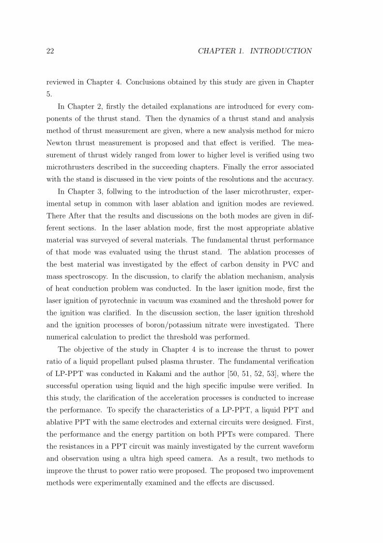
22 CHAPTER 1. INTRODUCTION
reviewed in Chapter 4. Conclusions obtained by this study are given in Chapter
5.
In Chapter 2, firstly the detailed explanations are introduced for every com-
ponents of the thrust stand. Then the dynamics of a thrust stand and analysis
method of thrust measurement are given, where a new analysis method for micro
Newton thrust measurement is proposed and that effect is verified. The mea-
surement of thrust widely ranged from lower to higher level is verified using two
microthrusters described in the succeeding chapters. Finally the error associated
with the stand is discussed in the view points of the resolutions and the accuracy.
In Chapter 3, follwing to the introduction of the laser microthruster, exper-
imental setup in common with laser ablation and ignition modes are reviewed.
There After that the results and discussions on the both modes are given in dif-
ferent sections. In the laser ablation mode, first the most appropriate ablative
material was surveyed of several materials. The fundamental thrust performance
of that mode was evaluated using the thrust stand. The ablation processes of
the best material was investigated by the effect of carbon density in PVC and
mass spectroscopy. In the discussion, to clarify the ablation mechanism, analysis
of heat conduction problem was conducted. In the laser ignition mode, first the
laser ignition of pyrotechnic in vacuum was examined and the threshold power for
the ignition was clarified. In the discussion section, the laser ignition threshold
and the ignition processes of boron/potassium nitrate were investigated. There
numerical calculation to predict the threshold was performed.
The objective of the study in Chapter 4 is to increase the thrust to power
ratio of a liquid propellant pulsed plasma thruster. The fundamental verification
of LP-PPT was conducted in Kakami and the author [50, 51, 52, 53], where the
successful operation using liquid and the high specific impulse were verified. In
this study, the clarification of the acceleration processes is conducted to increase
the performance. To specify the characteristics of a LP-PPT, a liquid PPT and
ablative PPT with the same electrodes and external circuits were designed. First,
the performance and the energy partition on both PPTs were compared. There
the resistances in a PPT circuit was mainly investigated by the current waveform
and observation using a ultra high speed camera. As a result, two methods to
improve the thrust to power ratio were proposed. The proposed two improvement
methods were experimentally examined and the effects are discussed.
Chapter 2
Thrust Stand for Micropropulsion
2.1 Introduction
Thrust measurement is most essential to validate the performance of thrusters.
However it is difficult to accurately measure extremely low thrust produced by
microthrusters. In the early stage of space development, few studies have ad-
dressed low thrust measurement of microthrusters, since the main focus at that
time was on developing primary propulsion systems. Stark et al.[54] performed
a study of low thrust measurement during the early 1970s. They developed a
torsional type thrust stand that oscillates horizontally and measured thrust of ion
engines ranging from 5 µN to 200 mN. Notwithstanding, that thrust stand was
quite complex and expensive. Recently, several studies of low thrust measurement
using a thrust stand have been done [55, 56, 57, 58, 59, 60] because of the in-
creasing interest in microthrusters. Haag [55] designed a thrust stand with the
same mechanism of Stark’s, but with simpler components. He measured impulse
of Pulsed Plasma Thruster (PPT) of 300 µNs. Cubbin et al.[56] developed an
optical interferometric proximeter for measuring impulse from PPTs within the
range of 100 µNs to 10 Ns. However, most of microthrusters produce lower im-
pulse (order of 10 µNs) than 100 µNs. Although there are other thrust stands
[57, 58, 59, 60] allowing measurement of such low thrust, most are specialized for
very lightweight thrusters.
23
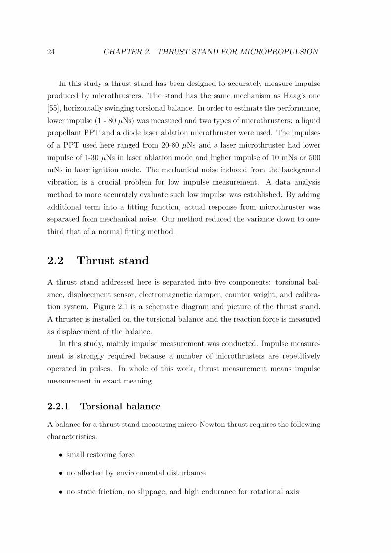
24 CHAPTER 2. THRUST STAND FOR MICROPROPULSION
In this study a thrust stand has been designed to accurately measure impulse
produced by microthrusters. The stand has the same mechanism as Haag’s one
[55], horizontally swinging torsional balance. In order to estimate the performance,
lower impulse (1 - 80 µNs) was measured and two types of microthrusters: a liquid
propellant PPT and a diode laser ablation microthruster were used. The impulses
of a PPT used here ranged from 20-80 µNs and a laser microthruster had lower
impulse of 1-30 µNs in laser ablation mode and higher impulse of 10 mNs or 500
mNs in laser ignition mode. The mechanical noise induced from the background
vibration is a crucial problem for low impulse measurement. A data analysis
method to more accurately evaluate such low impulse was established. By adding
additional term into a fitting function, actual response from microthruster was
separated from mechanical noise. Our method reduced the variance down to one-
third that of a normal fitting method.
2.2 Thrust stand
A thrust stand addressed here is separated into five components: torsional bal-
ance, displacement sensor, electromagnetic damper, counter weight, and calibra-
tion system. Figure 2.1 is a schematic diagram and picture of the thrust stand.
A thruster is installed on the torsional balance and the reaction force is measured
as displacement of the balance.
In this study, mainly impulse measurement was conducted. Impulse measure-
ment is strongly required because a number of microthrusters are repetitively
operated in pulses. In whole of this work, thrust measurement means impulse
measurement in exact meaning.
2.2.1 Torsional balance
A balance for a thrust stand measuring micro-Newton thrust requires the following
characteristics.
• small restoring force
• no affected by environmental disturbance
• no static friction, no slippage, and high endurance for rotational axis
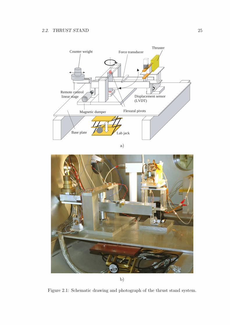
2.2. THRUST STAND 25
Magnetic dumper
Counter weight
Displacement sensor(LVDT)
Flexural pivots
Force transducerThruster
Remote controllinear stage
Base plate Lab jack
a)
b)
Figure 2.1: Schematic drawing and photograph of the thrust stand system.
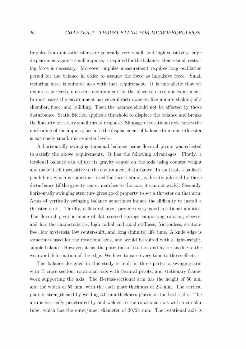
26 CHAPTER 2. THRUST STAND FOR MICROPROPULSION
Impulse from microthrusters are generally very small, and high sensitivity, large
displacement against small impulse, is required for the balance. Hence small restor-
ing force is necessary. Moreover impulse measurement requires long oscillation
period for the balance in order to assume the force as impulsive force. Small
restoring force is suitable also with that requirement. It is unrealistic that we
require a perfectly quiescent environment for the place to carry out experiment.
In most cases the environment has several disturbances, like minute shaking of a
chamber, floor, and building. Then the balance should not be affected by those
disturbance. Static friction applies a threshold to displace the balance and breaks
the linearity for a very small thrust response. Slippage of rotational axis causes the
misleading of the impulse, because the displacement of balance from microthruster
is extremely small, micro-meter levels.
A horizontally swinging torsional balance using flexural pivots was selected
to satisfy the above requirements. It has the following advantages. Firstly, a
torsional balance can adjust its gravity center on the axis using counter weight
and make itself insensitive to the environment disturbance. In contrast, a ballistic
pendulum, which is sometimes used for thrust stand, is directly affected by those
disturbance (if the gravity center matches to the axis, it can not work). Secondly,
horizontally swinging structure gives good property to set a thruster on that arm.
Arms of vertically swinging balance sometimes induce the difficulty to install a
thruster on it. Thirdly, a flexural pivot provides very good rotational abilities.
The flexural pivot is made of flat crossed springs supporting rotating sleeves,
and has the characteristics, high radial and axial stiffness, frictionless, stiction-
free, low hysterisis, low center-shift, and long (infinite) life time. A knife edge is
sometimes used for the rotational axis, and would be suited with a light-weight,
simple balance. However, it has the potentials of stiction and hysterisis due to the
wear and deformation of the edge. We have to care every time to those effects.
The balance designed in this study is built in three parts: a swinging arm
with H cross section, rotational axis with flexural pivots, and stationary frame-
work supporting the axis. The H-cross-sectional arm has the height of 50 mm
and the width of 55 mm, with the each plate thickness of 2.4 mm. The vertical
plate is strengthened by welding 3.0-mm-thickness-plates on the both sides. The
arm is vertically penetrated by and welded to the rotational axis with a circular
tube, which has the outer/inner diameter of 30/24 mm. The rotational axis is
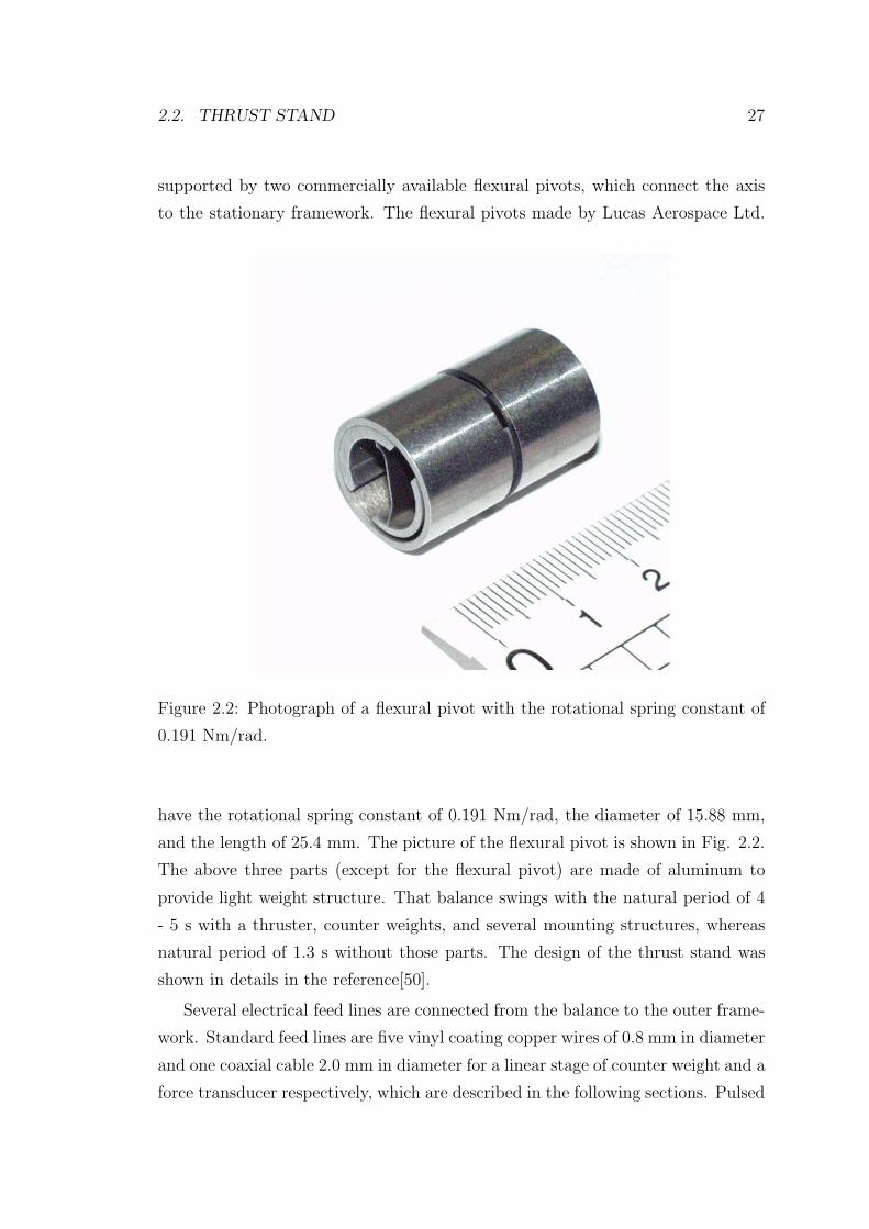
2.2. THRUST STAND 27
supported by two commercially available flexural pivots, which connect the axis
to the stationary framework. The flexural pivots made by Lucas Aerospace Ltd.
Figure 2.2: Photograph of a flexural pivot with the rotational spring constant of
0.191 Nm/rad.
have the rotational spring constant of 0.191 Nm/rad, the diameter of 15.88 mm,
and the length of 25.4 mm. The picture of the flexural pivot is shown in Fig. 2.2.
The above three parts (except for the flexural pivot) are made of aluminum to
provide light weight structure. That balance swings with the natural period of 4
- 5 s with a thruster, counter weights, and several mounting structures, whereas
natural period of 1.3 s without those parts. The design of the thrust stand was
shown in details in the reference[50].
Several electrical feed lines are connected from the balance to the outer frame-
work. Standard feed lines are five vinyl coating copper wires of 0.8 mm in diameter
and one coaxial cable 2.0 mm in diameter for a linear stage of counter weight and a
force transducer respectively, which are described in the following sections. Pulsed
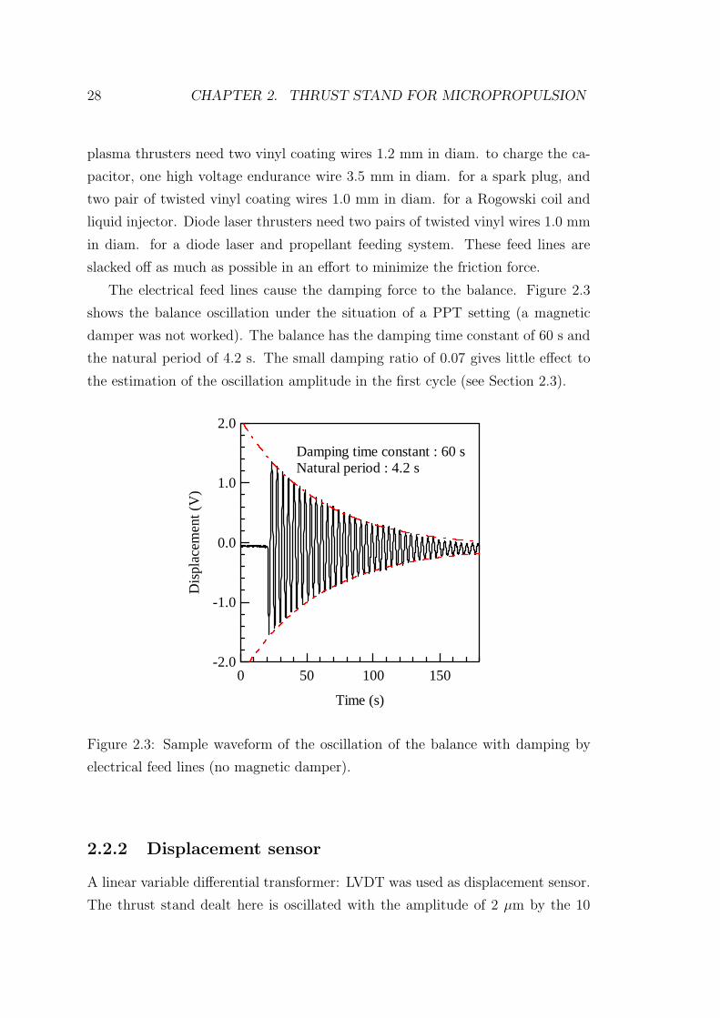
28 CHAPTER 2. THRUST STAND FOR MICROPROPULSION
plasma thrusters need two vinyl coating wires 1.2 mm in diam. to charge the ca-
pacitor, one high voltage endurance wire 3.5 mm in diam. for a spark plug, and
two pair of twisted vinyl coating wires 1.0 mm in diam. for a Rogowski coil and
liquid injector. Diode laser thrusters need two pairs of twisted vinyl wires 1.0 mm
in diam. for a diode laser and propellant feeding system. These feed lines are
slacked off as much as possible in an effort to minimize the friction force.
The electrical feed lines cause the damping force to the balance. Figure 2.3
shows the balance oscillation under the situation of a PPT setting (a magnetic
damper was not worked). The balance has the damping time constant of 60 s and
the natural period of 4.2 s. The small damping ratio of 0.07 gives little effect to
the estimation of the oscillation amplitude in the first cycle (see Section 2.3).
-2.0
-1.0
0.0
1.0
2.0
Dis
plac
emen
t (V
)
150100500
Time (s)
Damping time constant : 60 sNatural period : 4.2 s
Figure 2.3: Sample waveform of the oscillation of the balance with damping by
electrical feed lines (no magnetic damper).
2.2.2 Displacement sensor
A linear variable differential transformer: LVDT was used as displacement sensor.
The thrust stand dealt here is oscillated with the amplitude of 2 µm by the 10
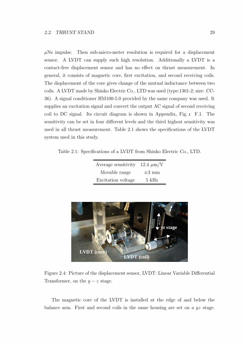
2.2. THRUST STAND 29
µNs impulse. Then sub-micro-meter resolution is required for a displacement
sensor. A LVDT can supply such high resolution. Additionally a LVDT is a
contact-free displacement sensor and has no effect on thrust measurement. In
general, it consists of magnetic core, first excitation, and second receiving coils.
The displacement of the core gives change of the mutual inductance between two
coils. A LVDT made by Shinko Electric Co., LTD was used (type:1301-2; size: CC-
36). A signal conditioner HM100-5.0 provided by the same company was used. It
supplies an excitation signal and convert the output AC signal of second receiving
coil to DC signal. Its circuit diagram is shown in Appendix, Fig. F.1. The
sensitivity can be set in four different levels and the third highest sensitivity was
used in all thrust measurement. Table 2.1 shows the specifications of the LVDT
system used in this study.
Table 2.1: Specifications of a LVDT from Shinko Electric Co., LTD.
Average sensitivity 12.4 µm/V
Movable range ±3 mm
Excitation voltage 5 kHz
LVDT (coil)LVDT (core)
yz stage
LVDT (coil)LVDT (core)
yz stage
Figure 2.4: Picture of the displacement sensor, LVDT: Linear Variable Differential
Transformer, on the y − z stage.
The magnetic core of the LVDT is installed at the edge of and below the
balance arm. First and second coils in the same housing are set on a yz stage.
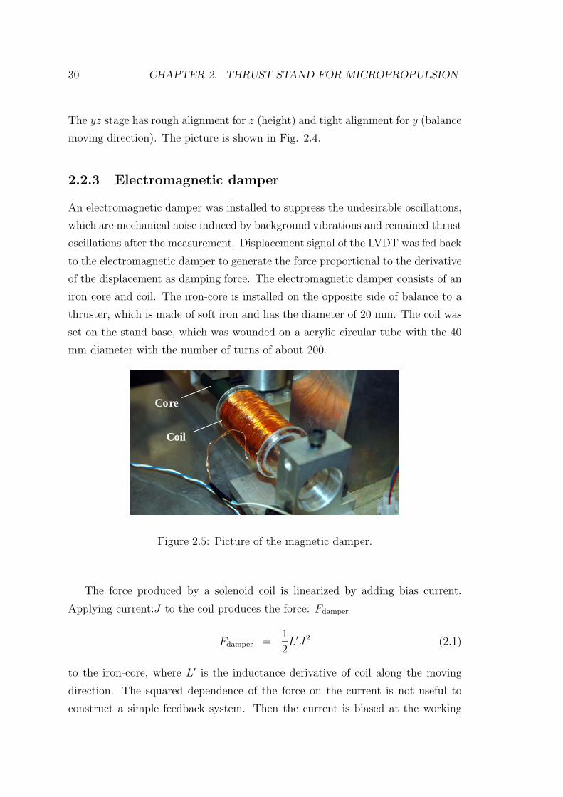
30 CHAPTER 2. THRUST STAND FOR MICROPROPULSION
The yz stage has rough alignment for z (height) and tight alignment for y (balance
moving direction). The picture is shown in Fig. 2.4.
2.2.3 Electromagnetic damper
An electromagnetic damper was installed to suppress the undesirable oscillations,
which are mechanical noise induced by background vibrations and remained thrust
oscillations after the measurement. Displacement signal of the LVDT was fed back
to the electromagnetic damper to generate the force proportional to the derivative
of the displacement as damping force. The electromagnetic damper consists of an
iron core and coil. The iron-core is installed on the opposite side of balance to a
thruster, which is made of soft iron and has the diameter of 20 mm. The coil was
set on the stand base, which was wounded on a acrylic circular tube with the 40
mm diameter with the number of turns of about 200.
Core
Coil
Core
Coil
Figure 2.5: Picture of the magnetic damper.
The force produced by a solenoid coil is linearized by adding bias current.
Applying current:J to the coil produces the force: Fdamper
Fdamper =1
2L′J2 (2.1)
to the iron-core, where L′ is the inductance derivative of coil along the moving
direction. The squared dependence of the force on the current is not useful to
construct a simple feedback system. Then the current is biased at the working
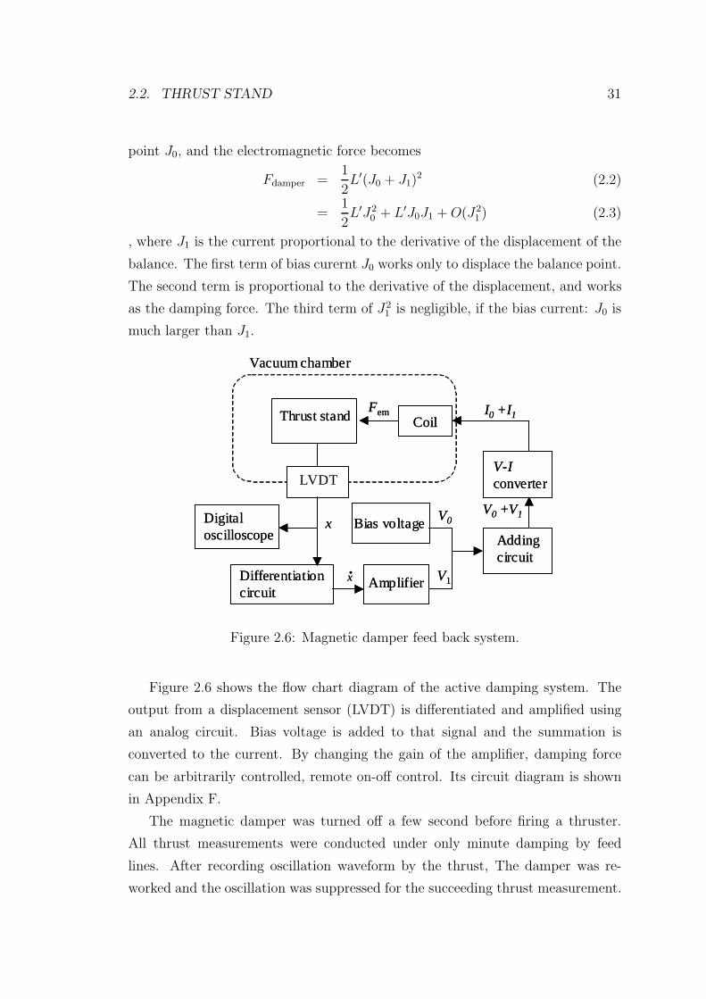
2.2. THRUST STAND 31
point J0, and the electromagnetic force becomes
Fdamper =1
2L′(J0 + J1)
2 (2.2)
=1
2L′J2
0 + L′J0J1 + O(J21 ) (2.3)
, where J1 is the current proportional to the derivative of the displacement of the
balance. The first term of bias curernt J0 works only to displace the balance point.
The second term is proportional to the derivative of the displacement, and works
as the damping force. The third term of J21 is negligible, if the bias current: J0 is
much larger than J1.
Bias voltageAdding circuit
V-Iconverter
Thrust stand
AmplifierDifferentiation circuit
Digital oscilloscope
Coil
Vacuum chamber
V1
LVDT
Fem
xV0
V0 +V1
I0 +I1
•x
Bias voltageAdding circuit
V-Iconverter
Thrust stand
AmplifierDifferentiation circuit
Digital oscilloscope
Coil
Vacuum chamber
V1
LVDT
Fem
xV0
V0 +V1
I0 +I1
•x
Figure 2.6: Magnetic damper feed back system.
Figure 2.6 shows the flow chart diagram of the active damping system. The
output from a displacement sensor (LVDT) is differentiated and amplified using
an analog circuit. Bias voltage is added to that signal and the summation is
converted to the current. By changing the gain of the amplifier, damping force
can be arbitrarily controlled, remote on-off control. Its circuit diagram is shown
in Appendix F.
The magnetic damper was turned off a few second before firing a thruster.
All thrust measurements were conducted under only minute damping by feed
lines. After recording oscillation waveform by the thrust, The damper was re-
worked and the oscillation was suppressed for the succeeding thrust measurement.
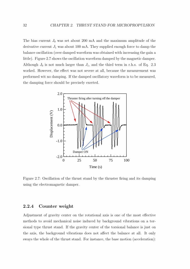
32 CHAPTER 2. THRUST STAND FOR MICROPROPULSION
The bias current J0 was set about 200 mA and the maximum amplitude of the
derivative current J1 was about 100 mA. They supplied enough force to damp the
balance oscillation (over damped waveform was obtained with increasing the gain a
little). Figure 2.7 shows the oscillation waveform damped by the magnetic damper.
Although J0 is not much larger than J1, and the third term in r.h.s. of Eq. 2.3
worked. However, the effect was not severe at all, because the measurement was
performed wit no damping. If the damped oscillatory waveform is to be measured,
the damping force should be precisely exerted.
-2.0
-1.0
0.0
1.0
2.0
Dis
plac
emen
t (V
)
1007550250
Time (s)
Thruster firing after turning off the damper
Damper ON
Figure 2.7: Oscillation of the thrust stand by the thruster firing and its damping
using the electromagnetic damper.
2.2.4 Counter weight
Adjustment of gravity center on the rotational axis is one of the most effective
methods to avoid mechanical noise induced by background vibrations on a tor-
sional type thrust stand. If the gravity center of the torsional balance is just on
the axis, the background vibrations does not affect the balance at all. It only
sways the whole of the thrust stand. For instance, the base motion (acceleration):
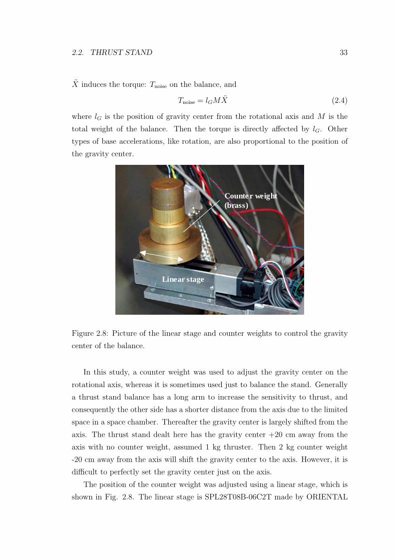
2.2. THRUST STAND 33
X induces the torque: Tnoise on the balance, and
Tnoise = lGMX (2.4)
where lG is the position of gravity center from the rotational axis and M is the
total weight of the balance. Then the torque is directly affected by lG. Other
types of base accelerations, like rotation, are also proportional to the position of
the gravity center.
Counte r weight(brass)
Linear stage
Counte r weight(brass)
Linear stage
Figure 2.8: Picture of the linear stage and counter weights to control the gravity
center of the balance.
In this study, a counter weight was used to adjust the gravity center on the
rotational axis, whereas it is sometimes used just to balance the stand. Generally
a thrust stand balance has a long arm to increase the sensitivity to thrust, and
consequently the other side has a shorter distance from the axis due to the limited
space in a space chamber. Thereafter the gravity center is largely shifted from the
axis. The thrust stand dealt here has the gravity center +20 cm away from the
axis with no counter weight, assumed 1 kg thruster. Then 2 kg counter weight
-20 cm away from the axis will shift the gravity center to the axis. However, it is
difficult to perfectly set the gravity center just on the axis.
The position of the counter weight was adjusted using a linear stage, which is
shown in Fig. 2.8. The linear stage is SPL28T08B-06C2T made by ORIENTAL
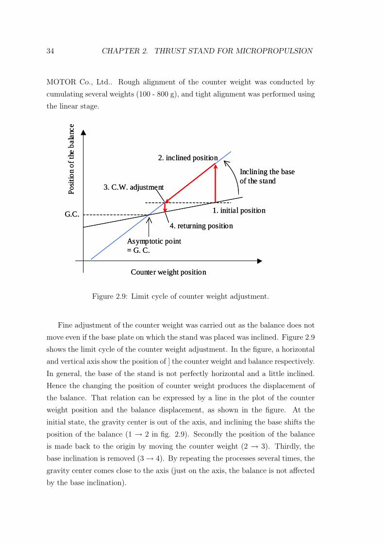
34 CHAPTER 2. THRUST STAND FOR MICROPROPULSION
MOTOR Co., Ltd.. Rough alignment of the counter weight was conducted by
cumulating several weights (100 - 800 g), and tight alignment was performed using
the linear stage.
G.C.
Counter weight position
Pos
itio
n o
f th
e b
alan
ce
Inclining the base of the stand
1. initial position
2. inclined position
3. C.W. adjustment
4. returning position
Asymptotic point= G. C.
G.C.
Counter weight position
Pos
itio
n o
f th
e b
alan
ce
Inclining the base of the stand
1. initial position
2. inclined position
3. C.W. adjustment
4. returning position
Asymptotic point= G. C.
Figure 2.9: Limit cycle of counter weight adjustment.
Fine adjustment of the counter weight was carried out as the balance does not
move even if the base plate on which the stand was placed was inclined. Figure 2.9
shows the limit cycle of the counter weight adjustment. In the figure, a horizontal
and vertical axis show the position of ] the counter weight and balance respectively.
In general, the base of the stand is not perfectly horizontal and a little inclined.
Hence the changing the position of counter weight produces the displacement of
the balance. That relation can be expressed by a line in the plot of the counter
weight position and the balance displacement, as shown in the figure. At the
initial state, the gravity center is out of the axis, and inclining the base shifts the
position of the balance (1 → 2 in fig. 2.9). Secondly the position of the balance
is made back to the origin by moving the counter weight (2 → 3). Thirdly, the
base inclination is removed (3 → 4). By repeating the processes several times, the
gravity center comes close to the axis (just on the axis, the balance is not affected
by the base inclination).
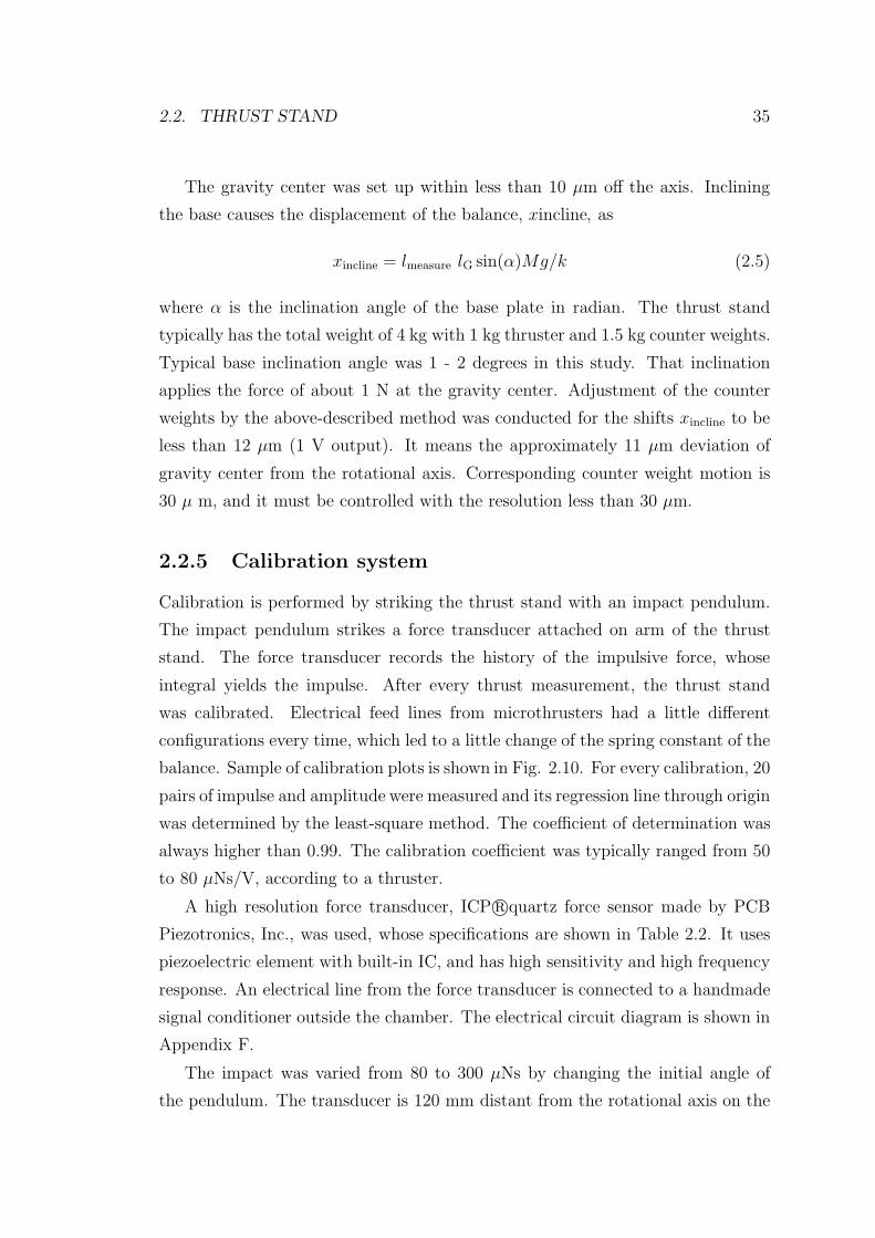
2.2. THRUST STAND 35
The gravity center was set up within less than 10 µm off the axis. Inclining
the base causes the displacement of the balance, xincline, as
xincline = lmeasure lG sin(α)Mg/k (2.5)
where α is the inclination angle of the base plate in radian. The thrust stand
typically has the total weight of 4 kg with 1 kg thruster and 1.5 kg counter weights.
Typical base inclination angle was 1 - 2 degrees in this study. That inclination
applies the force of about 1 N at the gravity center. Adjustment of the counter
weights by the above-described method was conducted for the shifts xincline to be
less than 12 µm (1 V output). It means the approximately 11 µm deviation of
gravity center from the rotational axis. Corresponding counter weight motion is
30 µ m, and it must be controlled with the resolution less than 30 µm.
2.2.5 Calibration system
Calibration is performed by striking the thrust stand with an impact pendulum.
The impact pendulum strikes a force transducer attached on arm of the thrust
stand. The force transducer records the history of the impulsive force, whose
integral yields the impulse. After every thrust measurement, the thrust stand
was calibrated. Electrical feed lines from microthrusters had a little different
configurations every time, which led to a little change of the spring constant of the
balance. Sample of calibration plots is shown in Fig. 2.10. For every calibration, 20
pairs of impulse and amplitude were measured and its regression line through origin
was determined by the least-square method. The coefficient of determination was
always higher than 0.99. The calibration coefficient was typically ranged from 50
to 80 µNs/V, according to a thruster.
A high resolution force transducer, ICP r©quartz force sensor made by PCB
Piezotronics, Inc., was used, whose specifications are shown in Table 2.2. It uses
piezoelectric element with built-in IC, and has high sensitivity and high frequency
response. An electrical line from the force transducer is connected to a handmade
signal conditioner outside the chamber. The electrical circuit diagram is shown in
Appendix F.
The impact was varied from 80 to 300 µNs by changing the initial angle of
the pendulum. The transducer is 120 mm distant from the rotational axis on the
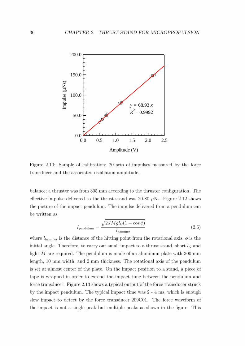
36 CHAPTER 2. THRUST STAND FOR MICROPROPULSION
200.0
150.0
100.0
50.0
0.0
Impu
lse
(µN
s)
2.52.01.51.00.50.0
Amplitude (V)
y = 68.93 x
R2 = 0.9992
Figure 2.10: Sample of calibration; 20 sets of impulses measured by the force
transducer and the associated oscillation amplitude.
balance; a thruster was from 305 mm according to the thruster configuration. The
effective impulse delivered to the thrust stand was 20-80 µNs. Figure 2.12 shows
the picture of the impact pendulum. The impulse delivered from a pendulum can
be written as
Ipendulum =
√2JMglG(1 − cos φ)
lhammer(2.6)
where lhammer is the distance of the hitting point from the rotational axis, φ is the
initial angle. Therefore, to carry out small impact to a thrust stand, short lG and
light M are required. The pendulum is made of an aluminum plate with 300 mm
length, 10 mm width, and 2 mm thickness. The rotational axis of the pendulum
is set at almost center of the plate. On the impact position to a stand, a piece of
tape is wrapped in order to extend the impact time between the pendulum and
force transducer. Figure 2.13 shows a typical output of the force transducer struck
by the impact pendulum. The typical impact time was 2 - 4 ms, which is enough
slow impact to detect by the force transducer 209C01. The force waveform of
the impact is not a single peak but multiple peaks as shown in the figure. This
2.2. THRUST STAND 37
Table 2.2: Specifications of a PCB force transducer 209C01.
Average sensitivity 490.7 mV/N
Maximum static force: compression 48.9 N
Broadband resolution (0 to 10 kHz) 0.09 mN
Low frequency response 0.5 Hz
Upper frequency limit 100 kHz
Discharge time constant ≥ 1 s
Electrical connection
Force Force transducer
Electrical connection
Force Force transducer
Figure 2.11: Picture of the force transducer 209C01.
multiple impacts would be caused by elastic oscillations of the pendulum during
the impact.
The impact pendulum was remotely controlled by rotating a propeller using
a DC motor. The remote controlling is necessary because the thrust stand has
very high sensitivity and is easily disturbed by the air convection from someone’s
closing it to operate the pendulum. The propeller can rotate up to the position of
a stopper stick and the pendulum is sustained at that position, that determines
the initial angle. The position of stopper stick was manually changed, which gives
varieties of the impulse. When the propeller was rotated in the counter direction,
the pendulum starts to swing and impacts the force transducer. Right after the
hitting, the propeller was returned to the initial position in order to prevent the
second hit of the pendulum to the stand.
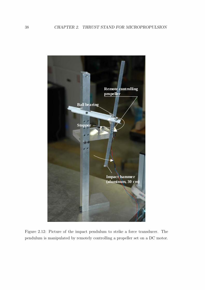
38 CHAPTER 2. THRUST STAND FOR MICROPROPULSION
Stopper
Remote controlling propeller
Impact hamme r(aluminum, 30 cm)
Ball bearing
Stopper
Remote controlling propeller
Impact hamme r(aluminum, 30 cm)
Ball bearing
Figure 2.12: Picture of the impact pendulum to strike a force transducer. The
pendulum is manipulated by remotely controlling a propeller set on a DC motor.
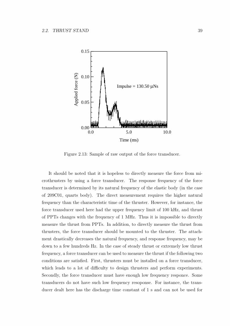
2.2. THRUST STAND 39
0.15
0.10
0.05
0.00
App
lied
forc
e (N
)
10.05.00.0
Time (ms)
Impulse = 130.50 µNs
Figure 2.13: Sample of raw output of the force transducer.
It should be noted that it is hopeless to directly measure the force from mi-
crothrusters by using a force transducer. The response frequency of the force
transducer is determined by its natural frequency of the elastic body (in the case
of 209C01, quarts body). The direct measurement requires the higher natural
frequency than the characteristic time of the thruster. However, for instance, the
force transducer used here had the upper frequency limit of 100 kHz, and thrust
of PPTs changes with the frequency of 1 MHz. Thus it is impossible to directly
measure the thrust from PPTs. In addition, to directly measure the thrust from
thrusters, the force transducer should be mounted to the thruster. The attach-
ment drastically decreases the natural frequency, and response frequency, may be
down to a few hundreds Hz. In the case of steady thrust or extremely low thrust
frequency, a force transducer can be used to measure the thrust if the following two
conditions are satisfied. First, thrusters must be installed on a force transducer,
which leads to a lot of difficulty to design thrusters and perform experiments.
Secondly, the force transducer must have enough low frequency responce. Some
transducers do not have such low frequency resoponse. For instance, the trans-
ducer dealt here has the discharge time constant of 1 s and can not be used for
40 CHAPTER 2. THRUST STAND FOR MICROPROPULSION
that use (discharge time is explained in Appendix A).
2.3 Dynamics of thrust stand
2.3.1 Basic analysis
The momentum equation for the torsional balance is
Jd2
dt2θ + c
d
dtθ + kθ = lforceF (t) (2.7)
where θ is the displacement angle of the balance, J is the moment of inertia of
the balance about the rotational axis, c is the coefficient of viscous damping for
rotation, k is the coefficient of torsional spring constant, and F (t) is the applied
force to the distance lforce away from the rotational axis. A displacement sensor
measures the distance lsensor away from the axis, and there displacement x can be
expressed as lsensorθ if θ 1. By introducing the natural angular frequency ω0
and the viscous coefficient µ, the momentum equation can be written as
d2
dt2x + 2µ
d
dtx + ω2
0x =lsensorlforce
JF (t) (2.8)
where ω0 =
√k
Jand µ =
c
2J(2.9)
In this study, only impulsive force with τforce τ0 or short time force with
τfroce < τ0 is measured, where τforce is the characteristic time of the applied force
and τ0 is the natural period of the balance, 2π/ω0. In the special case of the
impulsive force, F (t) = Iδ(t), and the stationary initial conditions, x(0) = 0 and
x(0) = 0 (short time force is considered in the succeeding section), the solution is
x(t) = A exp(−µt) sin(ω′t) (2.10)
where, A =lsensorlforce
Jω′ I and ω′ =√
ω20 − µ2 (2.11)
If there is no damping,
x(t) = A0 sin(ω0t) (2.12)
where, A0 =lsensorlforce
Jω0
I (2.13)
In the operations of the thrust stand, the electromagnetic damper was turned off
before the thruster fire, and the oscillation of the balance was measured under
2.3. DYNAMICS OF THRUST STAND 41
small damping due to some feed lines. Under such small damping effect, the
amplitude with damping A and without damping A0 are related as
A =lsensorlforceI
Jω0
√1 − ζ2
=1√
1 − ζ2A0 (2.14)
(
1 +ζ2
2
)A0 (ζ 1) (2.15)
ζ =µ
ω0(2.16)
where ζ is the damping ratio. Then the damping force affects the amplitude by
the second order, and small damping like ζ 1 can be neglected. Actually typical
value of ω0 and µ is 1.5 and 0.01 1/s, and the damping ratio is 0.007 1. The
associated difference between A and A0 less than 0.01 %. Therefore the damping
is neglected in the following sections, and Eq. (2.12) is used to obtain the impulse.
2.3.2 Analysis for short time force
Here let us to extend the above analysis to the short time force, that is, impulsive
force approximation is not valid but the time of applied force is shorter than the
natural period. The following force with finite pulse width:τpulse is considered
F (t) =
⎧⎨⎩ I/τpulse , 0 < t ≤ τpulse
0 , t ≤ 0, τpulse < t(2.17)
where I means the delivered total impulse. Then the solution for Eq. 2.9 under
the force Eq. 2.17 is
x(t) =
⎧⎪⎪⎪⎨⎪⎪⎪⎩
A01 − cosω0t
ω0τpulse, 0 < t ≤ τpulse
A0sin(ω0τpulse/2)
ω0τpusle/2sin ω0(t − τpulse/2) , t ≤ 0, τpulse < t
(2.18)
A thrust stand has the oscillation amplitude
Apulse = A0sin(ω0τpulse/2)
ω0τpusle/2(2.19)
The comparison of A0 and Apulse is shown in Fig. 2.14. If the applied force can
not be regarded as impulsive force, the oscillation amplitude should be corrected
according to Eq. (2.19). In the processes, however, we assumed the rectangular
waveform for the applied force and estimate its period. The uncertainties of those
lead to error of thrust measurement.
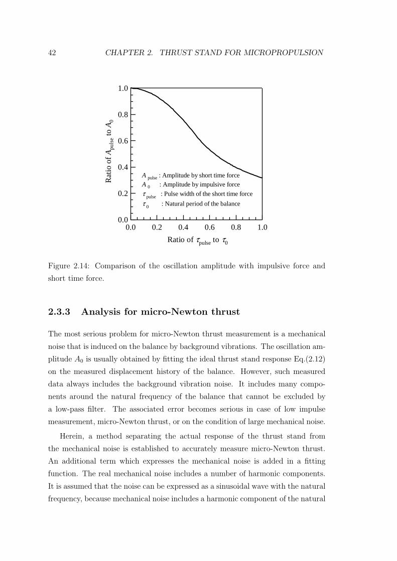
42 CHAPTER 2. THRUST STAND FOR MICROPROPULSION
1.0
0.8
0.6
0.4
0.2
0.0
Rat
io o
f A
puls
e to
A0
1.00.80.60.40.20.0
Ratio of τpulse to τ0
A pulse : Amplitude by short time force
A 0 : Amplitude by impulsive force
τ pulse : Pulse width of the short time force
τ 0 : Natural period of the balance
Figure 2.14: Comparison of the oscillation amplitude with impulsive force and
short time force.
2.3.3 Analysis for micro-Newton thrust
The most serious problem for micro-Newton thrust measurement is a mechanical
noise that is induced on the balance by background vibrations. The oscillation am-
plitude A0 is usually obtained by fitting the ideal thrust stand response Eq.(2.12)
on the measured displacement history of the balance. However, such measured
data always includes the background vibration noise. It includes many compo-
nents around the natural frequency of the balance that cannot be excluded by
a low-pass filter. The associated error becomes serious in case of low impulse
measurement, micro-Newton thrust, or on the condition of large mechanical noise.
Herein, a method separating the actual response of the thrust stand from
the mechanical noise is established to accurately measure micro-Newton thrust.
An additional term which expresses the mechanical noise is added in a fitting
function. The real mechanical noise includes a number of harmonic components.
It is assumed that the noise can be expressed as a sinusoidal wave with the natural
frequency, because mechanical noise includes a harmonic component of the natural
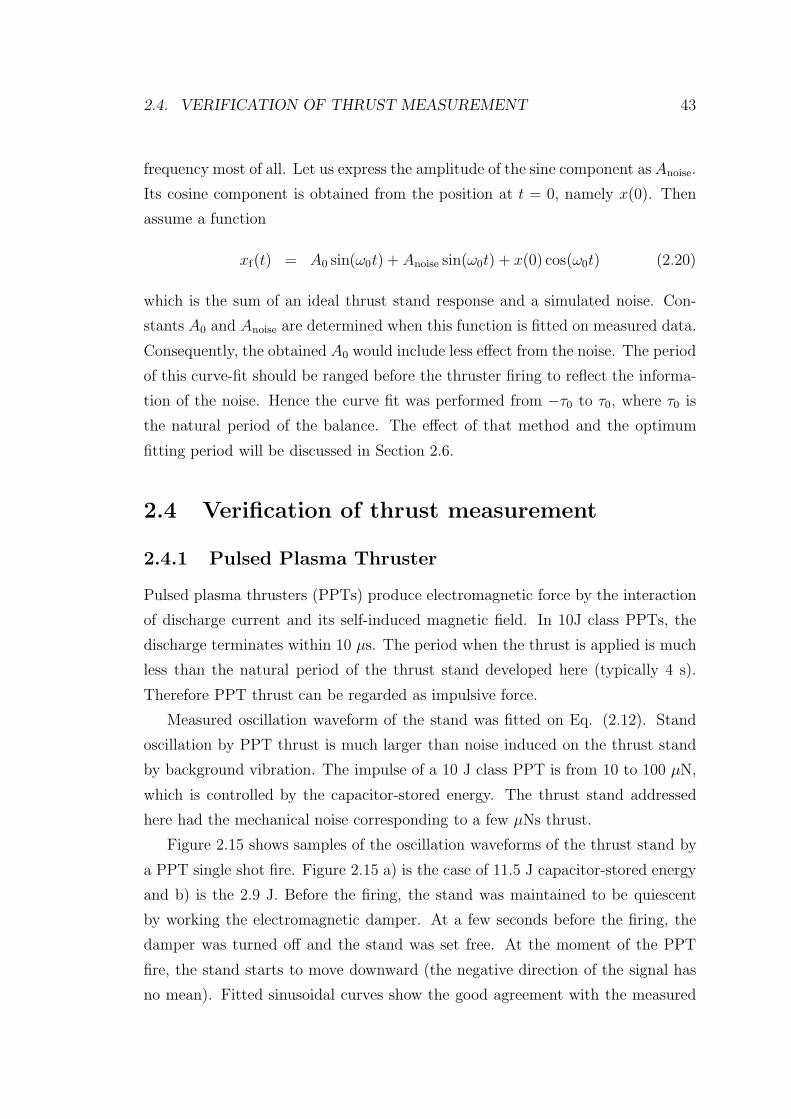
2.4. VERIFICATION OF THRUST MEASUREMENT 43
frequency most of all. Let us express the amplitude of the sine component as Anoise.
Its cosine component is obtained from the position at t = 0, namely x(0). Then
assume a function
xf(t) = A0 sin(ω0t) + Anoise sin(ω0t) + x(0) cos(ω0t) (2.20)
which is the sum of an ideal thrust stand response and a simulated noise. Con-
stants A0 and Anoise are determined when this function is fitted on measured data.
Consequently, the obtained A0 would include less effect from the noise. The period
of this curve-fit should be ranged before the thruster firing to reflect the informa-
tion of the noise. Hence the curve fit was performed from −τ0 to τ0, where τ0 is
the natural period of the balance. The effect of that method and the optimum
fitting period will be discussed in Section 2.6.
2.4 Verification of thrust measurement
2.4.1 Pulsed Plasma Thruster
Pulsed plasma thrusters (PPTs) produce electromagnetic force by the interaction
of discharge current and its self-induced magnetic field. In 10J class PPTs, the
discharge terminates within 10 µs. The period when the thrust is applied is much
less than the natural period of the thrust stand developed here (typically 4 s).
Therefore PPT thrust can be regarded as impulsive force.
Measured oscillation waveform of the stand was fitted on Eq. (2.12). Stand
oscillation by PPT thrust is much larger than noise induced on the thrust stand
by background vibration. The impulse of a 10 J class PPT is from 10 to 100 µN,
which is controlled by the capacitor-stored energy. The thrust stand addressed
here had the mechanical noise corresponding to a few µNs thrust.
Figure 2.15 shows samples of the oscillation waveforms of the thrust stand by
a PPT single shot fire. Figure 2.15 a) is the case of 11.5 J capacitor-stored energy
and b) is the 2.9 J. Before the firing, the stand was maintained to be quiescent
by working the electromagnetic damper. At a few seconds before the firing, the
damper was turned off and the stand was set free. At the moment of the PPT
fire, the stand starts to move downward (the negative direction of the signal has
no mean). Fitted sinusoidal curves show the good agreement with the measured
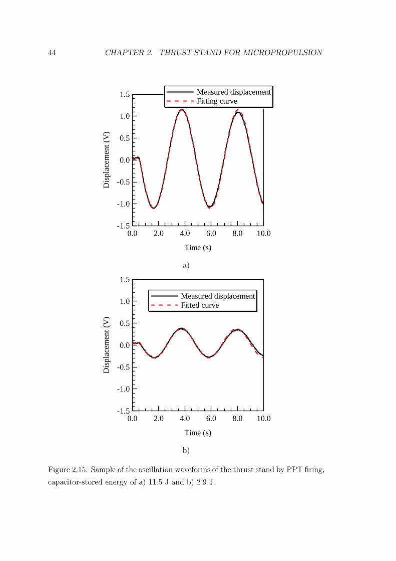
44 CHAPTER 2. THRUST STAND FOR MICROPROPULSION
-1.5
-1.0
-0.5
0.0
0.5
1.0
1.5
Dis
plac
emen
t (V
)
10.08.06.04.02.00.0
Time (s)
Measured displacement Fitting curve
a)
-1.5
-1.0
-0.5
0.0
0.5
1.0
1.5
Dis
plac
emen
t (V
)
10.08.06.04.02.00.0
Time (s)
Measured displacement Fitted curve
b)
Figure 2.15: Sample of the oscillation waveforms of the thrust stand by PPT firing,
capacitor-stored energy of a) 11.5 J and b) 2.9 J.
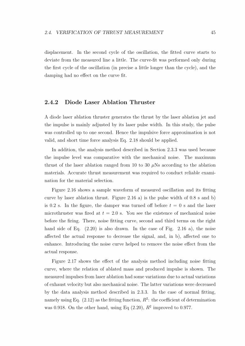
2.4. VERIFICATION OF THRUST MEASUREMENT 45
displacement. In the second cycle of the oscillation, the fitted curve starts to
deviate from the measured line a little. The curve-fit was performed only during
the first cycle of the oscillation (in precise a little longer than the cycle), and the
damping had no effect on the curve fit.
2.4.2 Diode Laser Ablation Thruster
A diode laser ablation thruster generates the thrust by the laser ablation jet and
the impulse is mainly adjusted by its laser pulse width. In this study, the pulse
was controlled up to one second. Hence the impulsive force approximation is not
valid, and short time force analysis Eq. 2.18 should be applied.
In addition, the analysis method described in Section 2.3.3 was used because
the impulse level was comparative with the mechanical noise. The maximum
thrust of the laser ablation ranged from 10 to 30 µNs according to the ablation
materials. Accurate thrust measurement was required to conduct reliable exami-
nation for the material selection.
Figure 2.16 shows a sample waveform of measured oscillation and its fitting
curve by laser ablation thrust. Figure 2.16 a) is the pulse width of 0.8 s and b)
is 0.2 s. In the figure, the damper was turned off before t = 0 s and the laser
microthruster was fired at t = 2.0 s. You see the existence of mechanical noise
before the firing. There, noise fitting curve, second and third terms on the right
hand side of Eq. (2.20) is also drawn. In the case of Fig. 2.16 a), the noise
affected the actual response to decrease the signal, and, in b), affected one to
enhance. Introducing the noise curve helped to remove the noise effect from the
actual response.
Figure 2.17 shows the effect of the analysis method including noise fitting
curve, where the relation of ablated mass and produced impulse is shown. The
measured impulses from laser ablation had some variations due to actual variations
of exhaust velocity but also mechanical noise. The latter variations were decreased
by the data analysis method described in 2.3.3. In the case of normal fitting,
namely using Eq. (2.12) as the fitting function, R2: the coefficient of determination
was 0.918. On the other hand, using Eq (2.20), R2 improved to 0.977.
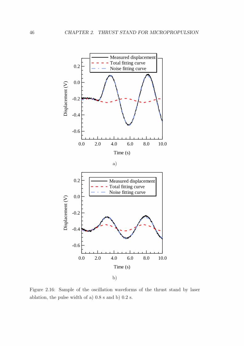
46 CHAPTER 2. THRUST STAND FOR MICROPROPULSION
-0.6
-0.4
-0.2
0.0
0.2D
ispl
acem
ent (
V)
10.08.06.04.02.00.0
Time (s)
Measured displacement Total fitting curve Noise fitting curve
a)
-0.6
-0.4
-0.2
0.0
0.2
Dis
plac
emen
t (V
)
10.08.06.04.02.00.0
Time (s)
Measured displacement Total fitting curve Noise fitting curve
b)
Figure 2.16: Sample of the oscillation waveforms of the thrust stand by laser
ablation, the pulse width of a) 0.8 s and b) 0.2 s.
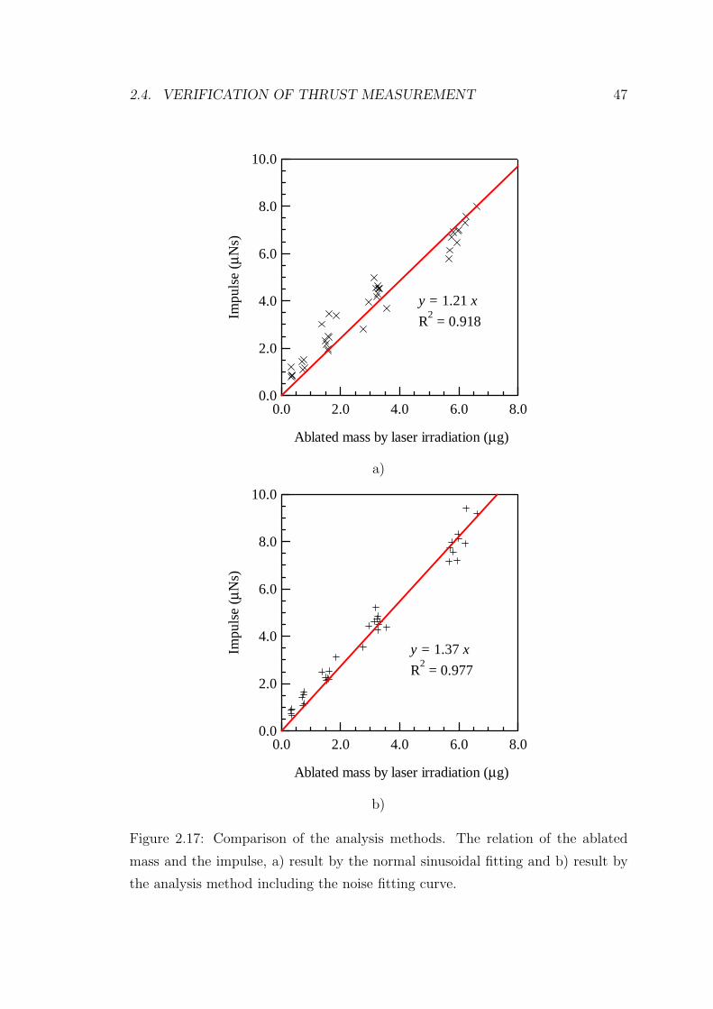
2.4. VERIFICATION OF THRUST MEASUREMENT 47
10.0
8.0
6.0
4.0
2.0
0.0
Impu
lse
(µN
s)
8.06.04.02.00.0
Ablated mass by laser irradiation (µg)
y = 1.21 x
R2 = 0.918
a)
10.0
8.0
6.0
4.0
2.0
0.0
Impu
lse
(µN
s)
8.06.04.02.00.0
Ablated mass by laser irradiation (µg)
y = 1.37 x
R2 = 0.977
b)
Figure 2.17: Comparison of the analysis methods. The relation of the ablated
mass and the impulse, a) result by the normal sinusoidal fitting and b) result by
the analysis method including the noise fitting curve.
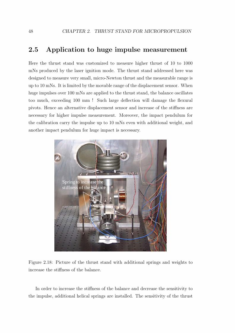
48 CHAPTER 2. THRUST STAND FOR MICROPROPULSION
2.5 Application to huge impulse measurement
Here the thrust stand was customized to measure higher thrust of 10 to 1000
mNs produced by the laser ignition mode. The thrust stand addressed here was
designed to measure very small, micro-Newton thrust and the measurable range is
up to 10 mNs. It is limited by the movable range of the displacement sensor. When
huge impulses over 100 mNs are applied to the thrust stand, the balance oscillates
too much, exceeding 100 mm ! Such large deflection will damage the flexural
pivots. Hence an alternative displacement sensor and increase of the stiffness are
necessary for higher impulse measurement. Moreover, the impact pendulum for
the calibration carry the impulse up to 10 mNs even with additional weight, and
another impact pendulum for huge impact is necessary.
Spring to increase the stiffness of the balanceSpring to increase the stiffness of the balance
Figure 2.18: Picture of the thrust stand with additional springs and weights to
increase the stiffness of the balance.
In order to increase the stiffness of the balance and decrease the sensitivity to
the impulse, additional helical springs are installed. The sensitivity of the thrust
2.5. APPLICATION TO HUGE IMPULSE MEASUREMENT 49
stand for micro-Newton thrust was about 0.2 µm/µNs, which means the 0.2 m
displacement in the case of 1 Ns. The displacement must be decreased at least
down to the level which flexural pivot can endure. The flexural pivot use here has
the cycle life of infinite when its deflection angle is within 10 degrees (under light
radial loading). It corresponds to the 50 mm displacement of the balance at 300
mm away from the axis. The sensitivity of the stand is inversely proportional to
square root of the stiffness and moment of inertia. Thus additional helical springs
and 2 - 4 kg weight were installed, shown in Fig. 2.18. Moreover, a thruster was
installed at the position of 120 mm. Those decreased the sensitivity of the thrust
stand by one tenth, namely down to about 0.02 m/Ns at the edge of the arm.
A laser displacement sensor was used to measure the large deflection of the
balance, because the LVDT used here cannot measure the displacement more
than 3 mm. It irradiates laser beam on a target and detects its scattering light.
Table 2.3 shows the specifications of the laser displacement sensor used here, LK-
500 made by Keyence Corporation. The laser beam was irradiated from outside
of the chamber through a view port, The sensor was operated using a long range
mode with low resolution due to the long distance by the chamber (see Table 2.3).
Displacement of the stand was measured at 320 mm away from the rotational axis
to increase the resolution.
Table 2.3: Specifications of a laser dispacement senosr (Keyence Corp.).
Model LK-500 (sensor head)
LK-2500 (amplifier)
Mode Fine Long
Detecting distance 350 mm 500 mm
Detecting range ±100 mm ±250 mm
Detecting distance 350 mm 500 mm
Light source Visible red semiconductor laser (690 nm)
Spot diameter D 0.7 mm D 0.3 mm
Resolution 10 µm 50 µm
Sensitivity 10 µm/mV 50 µm/mV
A new calibration hammer was designed for over 100 mNs impulse. The impact
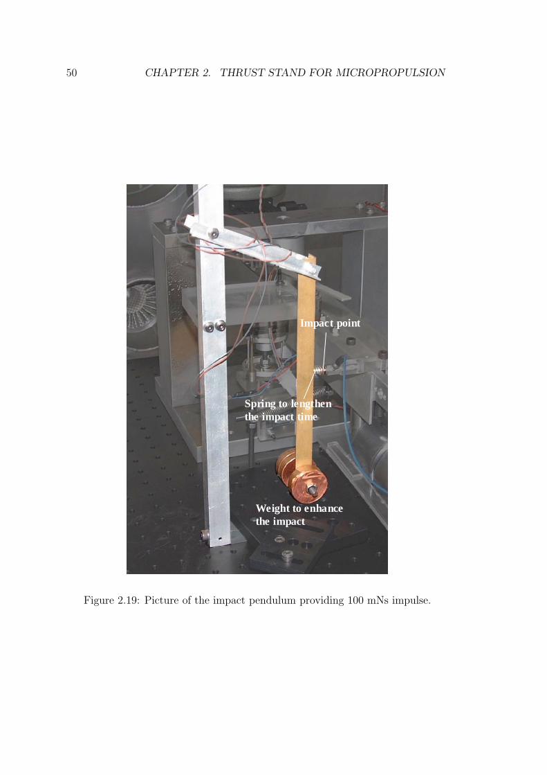
50 CHAPTER 2. THRUST STAND FOR MICROPROPULSION
Weight to enhance the impact
Spring to lengthen the impact time
Impact point
Weight to enhance the impact
Spring to lengthen the impact time
Impact point
Figure 2.19: Picture of the impact pendulum providing 100 mNs impulse.
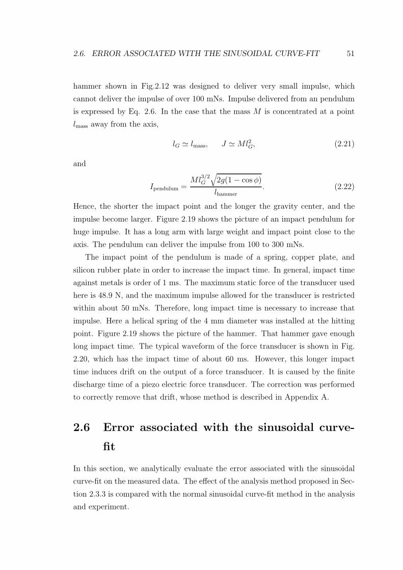
2.6. ERROR ASSOCIATED WITH THE SINUSOIDAL CURVE-FIT 51
hammer shown in Fig.2.12 was designed to deliver very small impulse, which
cannot deliver the impulse of over 100 mNs. Impulse delivered from an pendulum
is expressed by Eq. 2.6. In the case that the mass M is concentrated at a point
lmass away from the axis,
lG lmass, J Ml2G, (2.21)
and
Ipendulum =Ml
3/2G
√2g(1 − cos φ)
lhammer. (2.22)
Hence, the shorter the impact point and the longer the gravity center, and the
impulse become larger. Figure 2.19 shows the picture of an impact pendulum for
huge impulse. It has a long arm with large weight and impact point close to the
axis. The pendulum can deliver the impulse from 100 to 300 mNs.
The impact point of the pendulum is made of a spring, copper plate, and
silicon rubber plate in order to increase the impact time. In general, impact time
against metals is order of 1 ms. The maximum static force of the transducer used
here is 48.9 N, and the maximum impulse allowed for the transducer is restricted
within about 50 mNs. Therefore, long impact time is necessary to increase that
impulse. Here a helical spring of the 4 mm diameter was installed at the hitting
point. Figure 2.19 shows the picture of the hammer. That hammer gave enough
long impact time. The typical waveform of the force transducer is shown in Fig.
2.20, which has the impact time of about 60 ms. However, this longer impact
time induces drift on the output of a force transducer. It is caused by the finite
discharge time of a piezo electric force transducer. The correction was performed
to correctly remove that drift, whose method is described in Appendix A.
2.6 Error associated with the sinusoidal curve-
fit
In this section, we analytically evaluate the error associated with the sinusoidal
curve-fit on the measured data. The effect of the analysis method proposed in Sec-
tion 2.3.3 is compared with the normal sinusoidal curve-fit method in the analysis
and experiment.
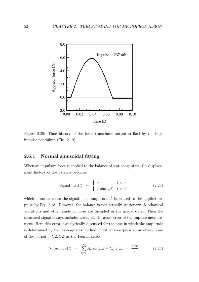
52 CHAPTER 2. THRUST STAND FOR MICROPROPULSION
8.0
6.0
4.0
2.0
0.0
-2.0
App
lied
for
ce (
N)
0.100.080.060.040.020.00
Time (s)
Impulse = 237 mNs
Figure 2.20: Time history of the force transducer output striked by the huge
impulse pendulum (Fig. 2.19).
2.6.1 Normal sinusoidal fitting
When an impulsive force is applied to the balance of stationary state, the displace-
ment history of the balance becomes
Signal : xs(t) =
⎧⎨⎩ 0 t < 0
A sin(ω0t) t > 0(2.23)
which is measured as the signal. The amplitude A is related to the applied im-
pulse by Eq. 2.13. However, the balance is not actually stationary. Mechanical
vibrations and other kinds of noise are included in the actual data. Then the
measured signal always includes noise, which causes error of the impulse measure-
ment. Here this error is analytically discussed for the case in which the amplitude
is determined by the least-squares method. First let us express an arbitrary noise
of the period [−l/2, l/2] as the Fourier series,
Noise : xN(t) =∞∑
n=1
An sin(ωnt + δn) , ωn =2nπ
l(2.24)
2.6. ERROR ASSOCIATED WITH THE SINUSOIDAL CURVE-FIT 53
Amplitudes and phases of its harmonic components are determined from the
Fourier series of the noise data. The actually measured signal is the summation
of the ideal wave and noise waves, that is xs(t) + xN(t). When a fitting function:
Fitting curve : xf (t) = Af sin(ω0t) (2.25)
is fitted on the data with the period [0, NT0], where N is the arbitrary natural
number (N = 1, 2, 3 . . .), the squared deviations is
Π ≡∫ NT0
0dt [xs(t) + xN(t) − xf (t)]2 (2.26)
=∫ NT0
0dt
[(A − Af) sin ω0t +
∞∑n=1
An sin(ωnt + δn)
]2
(2.27)
Differentiating Eq.2.27 with respect to Af and setting it equal to 0 give the am-
plitude Af such that the squared-deviations achieves the minimum value. After a
few algebraic manipulations, the amplitude is obtained as
Af = A +∞∑
n=1
AnI(0,NT0)n (2.28)
I (T1,T2)n ≡ 2
T0
∫ T2
T1
sinω0t sin(ωnt + δn)dt (2.29)
where the first term of Eq. 2.28 is the actual amplitude and the second term
indicates the error caused by the noise Eq. 2.24. Our interest is in the ensemble
averages and variances of the obtained amplitude. Phases of the harmonic com-
ponents are random within 0 to 2π because the noise is assumed to be a random
process. Hence,
< sin(ωnt + δn) > = 0 (2.30)
< I (0,NT0)n > = 0 (2.31)
where < · > denotes the ensemble average; hence
< Af > = A (2.32)
The mean value determined by the least-squares method agrees with the real value
(trivial). Next, we calculate the mean square to obtain the variance.
< A2f > = <
(A +
∞∑n=1
AnI(0,NT0)n
)(A +
∞∑m=1
AmI (0,NT0)m
)> (2.33)
54 CHAPTER 2. THRUST STAND FOR MICROPROPULSION
= A2 +∞∑
n,m
< AnAm >< I (0,NT0)n I (0,NT0)
m > (2.34)
= A2 +∞∑n
< A2n > w(0,NT0)(ωn/ω0) (2.35)
w(0,NT0)(x) ≡ 2
N2π2
sin2(Nπx)
(1 − x2)2(2.36)
where
< I (0,NT0)n > = 0 (2.37)
< I (0,NT0)n I (0,NT0)
m > and =
⎧⎨⎩ 0 , n = m
w(0,NT0)(ωn/ω0) , n = m(2.38)
were used. To consider non periodic random process noise, let l → ∞. Then the
summation becomes an integral. Using the relation
liml→∞
l
4< A2
n > = 2πS(ω) (2.39)
the means-squared of the amplitude becomes a power spectrum density S(ω). The
definition and detailed explanation on the power spectrum density is described in
the reference[61]. Hence,
1
2< A2
f > =1
2A2 +
∫ ∞
−∞w(0,NT0) (ω/ω0) S(ω)dω (2.40)
Derivations of Eqs. 2.39 and 2.40 are shown in Appendix C.
Finally, we obtain the expression of the variance
σ2 =∫ ∞
−∞w(0,NT0) (ω/ω0)S(ω)dω (2.41)
Generally the integral of power spectrum of the random process gives its mean-
square value of it. The function w(0,NT )(x) can be regarded as a weighting function,
which is shown in Fig. 2.21. Therefore the weighting function for N = 1: w(0,T0)(x)
has a large peak at x = 0.8374 with width of 0.4 to 1.3. Hence, noise near the
natural frequency contributes greatly to the variance. In contrast, the higher
frequency component contributes little to the curve fit error because the function
decreases biquadratically (see Eq. 2.36). The position of the peak shifts toward
x = 1 as the fitting period increases, with touching on the curve of N = 1; the
peak width becomes narrow.
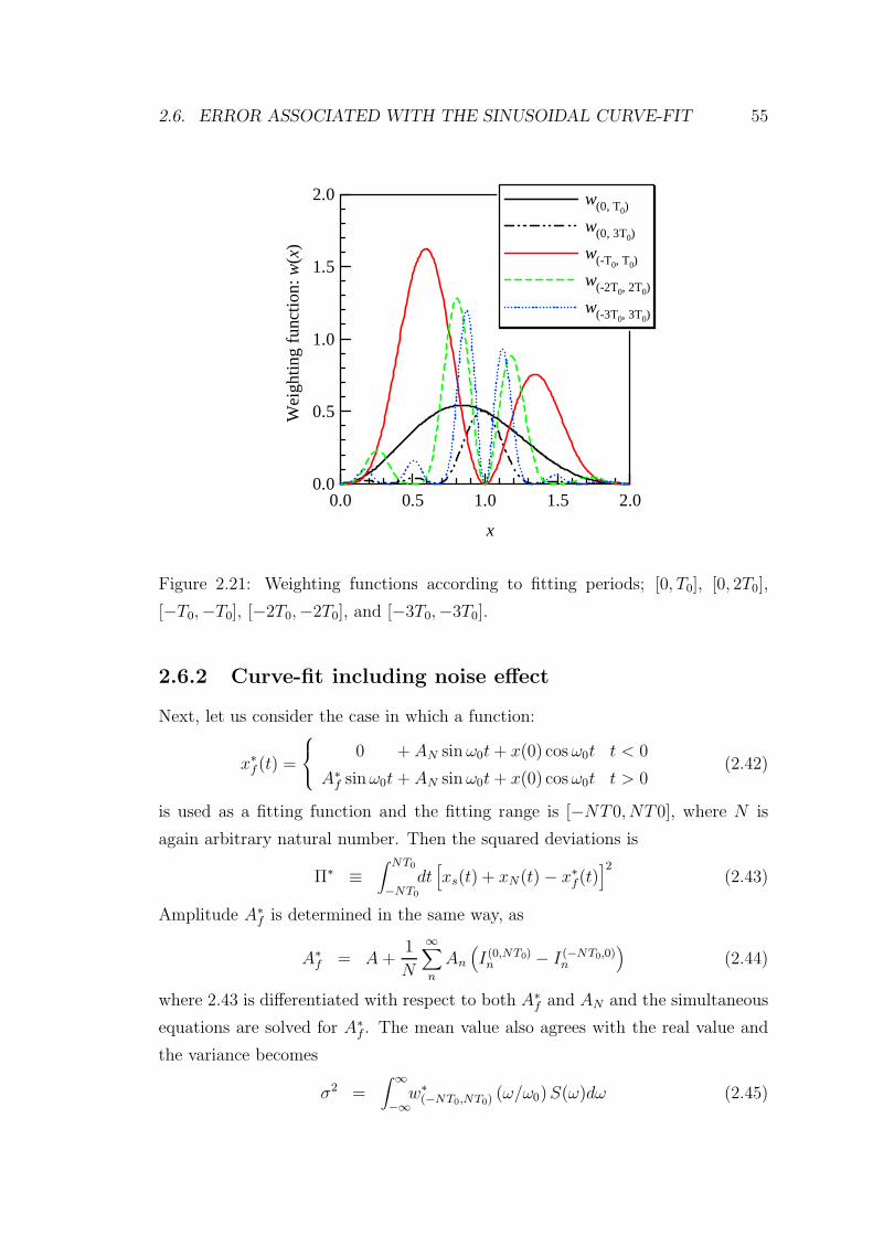
2.6. ERROR ASSOCIATED WITH THE SINUSOIDAL CURVE-FIT 55
2.0
1.5
1.0
0.5
0.0
Wei
ghtin
g fu
ncti
on: w
(x)
2.01.51.00.50.0
x
w(0, T0)
w(0, 3T0)
w(-T0, T0)
w(-2T0, 2T0)
w(-3T0, 3T0)
Figure 2.21: Weighting functions according to fitting periods; [0, T0], [0, 2T0],
[−T0,−T0], [−2T0,−2T0], and [−3T0,−3T0].
2.6.2 Curve-fit including noise effect
Next, let us consider the case in which a function:
x∗f (t) =
⎧⎨⎩ 0 + AN sin ω0t + x(0) cos ω0t t < 0
A∗f sinω0t + AN sin ω0t + x(0) cos ω0t t > 0
(2.42)
is used as a fitting function and the fitting range is [−NT 0, NT 0], where N is
again arbitrary natural number. Then the squared deviations is
Π∗ ≡∫ NT0
−NT0
dt[xs(t) + xN(t) − x∗
f(t)]2
(2.43)
Amplitude A∗f is determined in the same way, as
A∗f = A +
1
N
∞∑n
An
(I (0,NT0)n − I (−NT0,0)
n
)(2.44)
where 2.43 is differentiated with respect to both A∗f and AN and the simultaneous
equations are solved for A∗f . The mean value also agrees with the real value and
the variance becomes
σ2 =∫ ∞
−∞w∗
(−NT0,NT0)(ω/ω0)S(ω)dω (2.45)
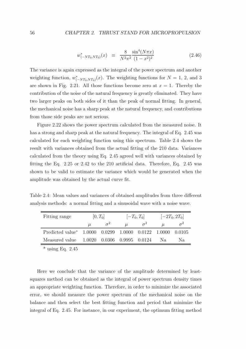
56 CHAPTER 2. THRUST STAND FOR MICROPROPULSION
w∗(−NT0,NT0)
(x) ≡ 8
N2π2
sin4(Nπx)
(1 − x2)2(2.46)
The variance is again expressed as the integral of the power spectrum and another
weighting function, w∗(−NT0,NT0)
(x). The weighting functions for N = 1, 2, and 3
are shown in Fig. 2.21. All those functions become zero at x = 1. Thereby the
contribution of the noise of the natural frequency is greatly eliminated. They have
two larger peaks on both sides of it than the peak of normal fitting. In general,
the mechanical noise has a sharp peak at the natural frequency, and contributions
from those side peaks are not serious.
Figure 2.22 shows the power spectrum calculated from the measured noise. It
has a strong and sharp peak at the natural frequency. The integral of Eq. 2.45 was
calculated for each weighting function using this spectrum. Table 2.4 shows the
result with variances obtained from the actual fitting of the 210 data. Variances
calculated from the theory using Eq. 2.45 agreed well with variances obtained by
fitting the Eq. 2.25 or 2.42 to the 210 artificial data. Therefore, Eq. 2.45 was
shown to be valid to estimate the variance which would be generated when the
amplitude was obtained by the actual curve fit.
Table 2.4: Mean values and variances of obtained amplitudes from three different
analysis methods: a normal fitting and a sinusoidal wave with a noise wave.
Fitting range [0, T0] [−T0, T0] [−2T0, 2T0]
µ σ2 µ σ2 µ σ2
Predicted value∗ 1.0000 0.0299 1.0000 0.0122 1.0000 0.0105
Measured value 1.0020 0.0306 0.9995 0.0124 Na Na
* using Eq. 2.45
Here we conclude that the variance of the amplitude determined by least-
squares method can be obtained as the integral of power spectrum density times
an appropriate weighting function. Therefore, in order to minimize the associated
error, we should measure the power spectrum of the mechanical noise on the
balance and then select the best fitting function and period that minimize the
integral of Eq. 2.45. For instance, in our experiment, the optimum fitting method
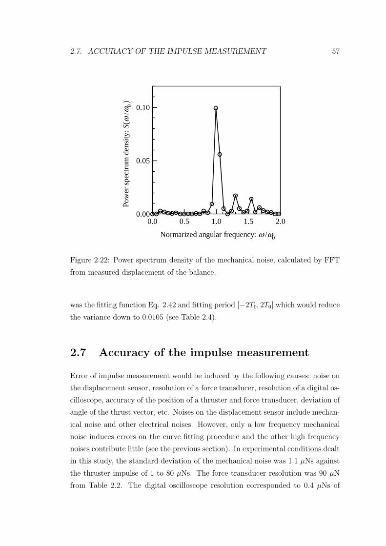
2.7. ACCURACY OF THE IMPULSE MEASUREMENT 57
0.10
0.05
0.00
Pow
er s
pect
rum
den
sity
: S(ω
/ω0
)
2.01.51.00.50.0
Normarized angular frequency: ω /ω0
Figure 2.22: Power spectrum density of the mechanical noise, calculated by FFT
from measured displacement of the balance.
was the fitting function Eq. 2.42 and fitting period [−2T0, 2T0] which would reduce
the variance down to 0.0105 (see Table 2.4).
2.7 Accuracy of the impulse measurement
Error of impulse measurement would be induced by the following causes: noise on
the displacement sensor, resolution of a force transducer, resolution of a digital os-
cilloscope, accuracy of the position of a thruster and force transducer, deviation of
angle of the thrust vector, etc. Noises on the displacement sensor include mechan-
ical noise and other electrical noises. However, only a low frequency mechanical
noise induces errors on the curve fitting procedure and the other high frequency
noises contribute little (see the previous section). In experimental conditions dealt
in this study, the standard deviation of the mechanical noise was 1.1 µNs against
the thruster impulse of 1 to 80 µNs. The force transducer resolution was 90 µN
from Table 2.2. The digital oscilloscope resolution corresponded to 0.4 µNs of
58 CHAPTER 2. THRUST STAND FOR MICROPROPULSION
impulse. Both position of the force transducer and the angle of the thrust vector
axis of thruster were set within the accuracy of 0.3 mm and 5 degrees respectively.
First, presume an error caused by a mechanical noise, inducing shot to shot
variation when the amplitude of the balance is estimated from displacement data.
The accuracy of the amplitude determined by the curve fitting under arbitrary
noise was discussed theoretically in the above section. According to that result, if
normal sinusoidal fitting is performed, the associated error of the amplitude would
be 1.0 µNs. In contrast, if a fitting function of Eq. 2.20 is used, this error would
be decreased down to 0.6 µNs of impulse
Secondly, the accuracy of the calibration constant is addressed. It is given as
α =Ipendulumlsensor
Alpendulum(2.47)
where Ipendulum is impulse measured by the force transducer and lpendulum is its
position from the rotating center of the balance. The uncertainty of the averaged
value of Ipendulum over A can be reduced by increasing the number of measurement
points. Actually the measurement was performed about 20 times in the every ex-
periment, and those effects was found almost negligible. Uncertainty arose mainly
from the error of position measurements of lsensor and lpendulum. Consequently,
a typical calibration constant was 49.5±1.2 µNs/V. The total error of impulse
measurement is affected by the errors of both calibration constant and measured
amplitude,
∆I2 = ∆α2A2 + ∆A2α2 (2.48)
where ∆A and ∆α are the uncertainties of the amplitude and calibration constant
respectively. If ∆A/A > ∆α/α, the amplitude error becomes dominant; thereby,
the improved analysis method, curve fit including noise data, would be valid, and
vice versa. For instance, for impulse of 10 µNs, where the error from the measured
amplitude was dominant, the total error would be 1.0 µNs if normal sinusoidal
fitting were used. If the fitting function Eq. 2.20 were used, this value would be
decreased down to 0.6 µNs. On the other hand, for impulse of 100 µNs, the total
error was 2.6 µNs, where the error caused by calibration constant was dominant.
Accuracy of positions of the thruster and force transducer becomes particularly
important.
2.8. CONCLUSIONS OF CHAPTER 2 59
2.8 Conclusions of Chapter 2
In this chapter, a thrust stand for micropropulsion was developed and the following
conclusions were obtained.
• It is shown that the thrust stand has high resolution and high accuracy and it
can be applied for wide varieties of micropropulsions. The resolution was less
than 1.0 µNs and the accuracy is within 2.0 %. That thrust measurement
was examined using thrusters of the weight up to 2.0 kg (the stand was
designed to endure thruster weight over 10 kg). The measured thrust was
1 to 30 µNs in the laser ablation thrustr, 20 to 100 µNs in a pulsed plasma
thruster, and 10 and 500 mNs in a laser ignition thruster.
• To increase the resolution on micro-Newton thrust measurement, accurate
adjustment of the gravity center (<10 µ m) and effective damping of the
stand are essential.
• A fitting-curve was newly proposed to removing the mechanical noises in-
duced by background vibrations. That effect was analytically clarified and
experimentally verified.

Chapter 3
Dual Propulsive Mode Laser
Microthruster
3.1 Introduction
3.1.1 Micropropulsions for 1-10 kg Microspacecraft
Recently several laboratory and flight models of 1-10 kg class microspacecraft have
been developed and successfully launched by several researchers and universities’
students team[2, 3, 4, 5]. Those microspacecraft have conducted the observation of
the earth, measurement of the upper atmosphere, and so on. Increasing activities
to develop such 1-10 kg microspacecraft is motivated by their reasonable cost
for the launching and developing. They are manufactured using commercially
available components, in contrast to highly functional spacecraft using, extremely
expensive, special components. The microspacecraft are launched as piggy-back
satellite or using an economical rocket of Russia. They make universities’ student
teams possible to design, fabricate, and launch the microspacecraft, which is also
expected as an effective educational course.
In the current stage, however, most of such microspacecraft conducts only
very simple missions as demonstrations. Severe limit of weight and size restricts
the functions of spacecraft. Especially lack of the propulsion systems make the
mission variety to be limited. In order to enable advanced microspacecraft mis-
sions, such as formation flying, a microthruster suitable for such microspacecraft
is needed. The micropropulsion installed to the spacecraft would realize a number
61
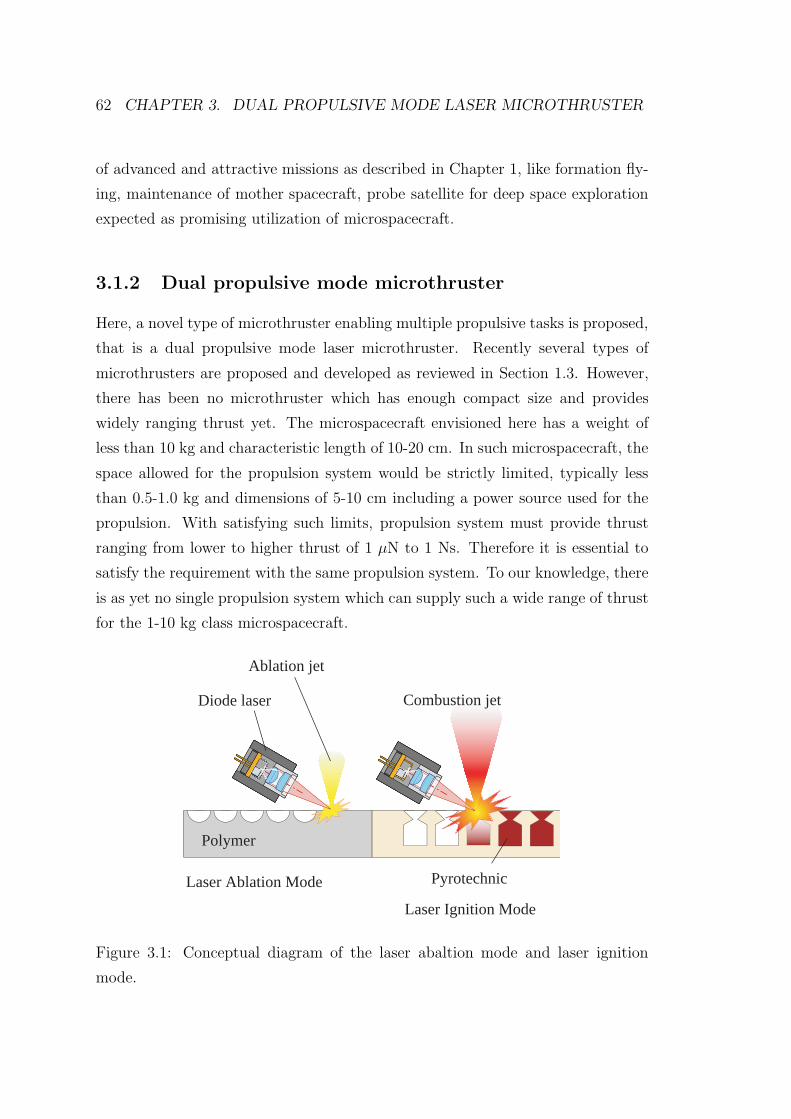
62 CHAPTER 3. DUAL PROPULSIVE MODE LASER MICROTHRUSTER
of advanced and attractive missions as described in Chapter 1, like formation fly-
ing, maintenance of mother spacecraft, probe satellite for deep space exploration
expected as promising utilization of microspacecraft.
3.1.2 Dual propulsive mode microthruster
Here, a novel type of microthruster enabling multiple propulsive tasks is proposed,
that is a dual propulsive mode laser microthruster. Recently several types of
microthrusters are proposed and developed as reviewed in Section 1.3. However,
there has been no microthruster which has enough compact size and provides
widely ranging thrust yet. The microspacecraft envisioned here has a weight of
less than 10 kg and characteristic length of 10-20 cm. In such microspacecraft, the
space allowed for the propulsion system would be strictly limited, typically less
than 0.5-1.0 kg and dimensions of 5-10 cm including a power source used for the
propulsion. With satisfying such limits, propulsion system must provide thrust
ranging from lower to higher thrust of 1 µN to 1 Ns. Therefore it is essential to
satisfy the requirement with the same propulsion system. To our knowledge, there
is as yet no single propulsion system which can supply such a wide range of thrust
for the 1-10 kg class microspacecraft.
Laser Ablation Mode
Laser Ignition Mode
Diode laser Combustion jet
Ablation jet
Pyrotechnic
Polymer
Figure 3.1: Conceptual diagram of the laser abaltion mode and laser ignition
mode.
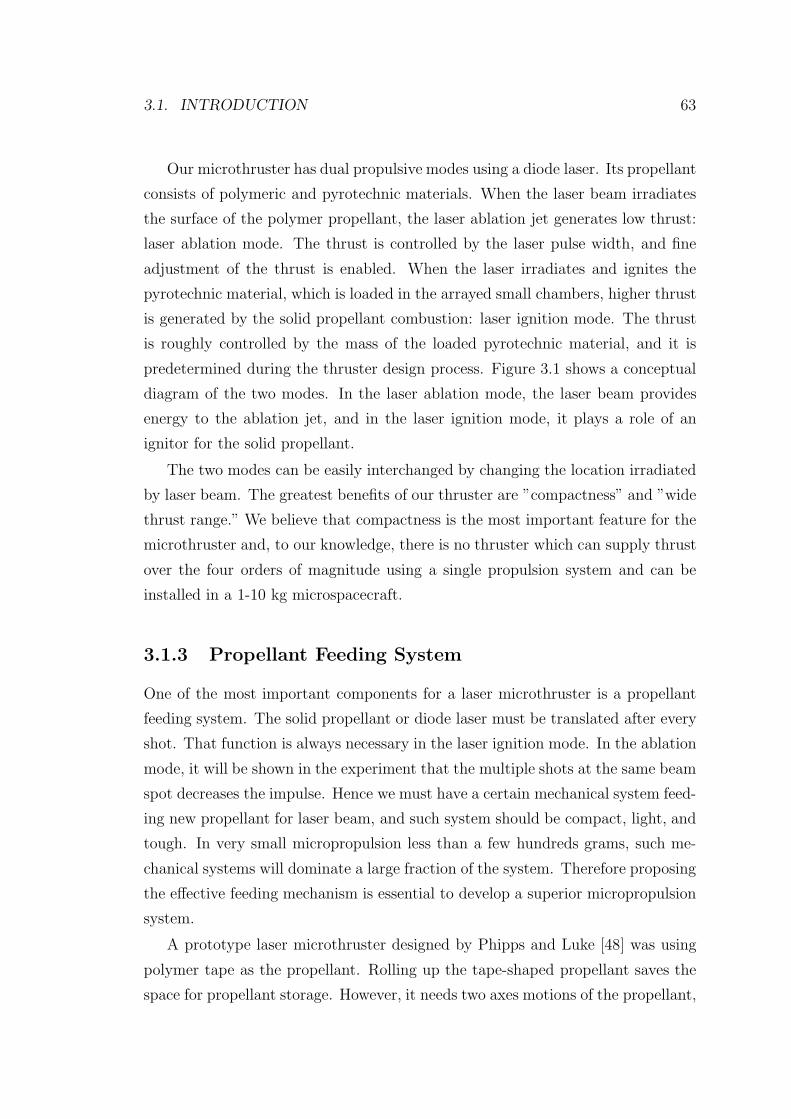
3.1. INTRODUCTION 63
Our microthruster has dual propulsive modes using a diode laser. Its propellant
consists of polymeric and pyrotechnic materials. When the laser beam irradiates
the surface of the polymer propellant, the laser ablation jet generates low thrust:
laser ablation mode. The thrust is controlled by the laser pulse width, and fine
adjustment of the thrust is enabled. When the laser irradiates and ignites the
pyrotechnic material, which is loaded in the arrayed small chambers, higher thrust
is generated by the solid propellant combustion: laser ignition mode. The thrust
is roughly controlled by the mass of the loaded pyrotechnic material, and it is
predetermined during the thruster design process. Figure 3.1 shows a conceptual
diagram of the two modes. In the laser ablation mode, the laser beam provides
energy to the ablation jet, and in the laser ignition mode, it plays a role of an
ignitor for the solid propellant.
The two modes can be easily interchanged by changing the location irradiated
by laser beam. The greatest benefits of our thruster are ”compactness” and ”wide
thrust range.” We believe that compactness is the most important feature for the
microthruster and, to our knowledge, there is no thruster which can supply thrust
over the four orders of magnitude using a single propulsion system and can be
installed in a 1-10 kg microspacecraft.
3.1.3 Propellant Feeding System
One of the most important components for a laser microthruster is a propellant
feeding system. The solid propellant or diode laser must be translated after every
shot. That function is always necessary in the laser ignition mode. In the ablation
mode, it will be shown in the experiment that the multiple shots at the same beam
spot decreases the impulse. Hence we must have a certain mechanical system feed-
ing new propellant for laser beam, and such system should be compact, light, and
tough. In very small micropropulsion less than a few hundreds grams, such me-
chanical systems will dominate a large fraction of the system. Therefore proposing
the effective feeding mechanism is essential to develop a superior micropropulsion
system.
A prototype laser microthruster designed by Phipps and Luke [48] was using
polymer tape as the propellant. Rolling up the tape-shaped propellant saves the
space for propellant storage. However, it needs two axes motions of the propellant,
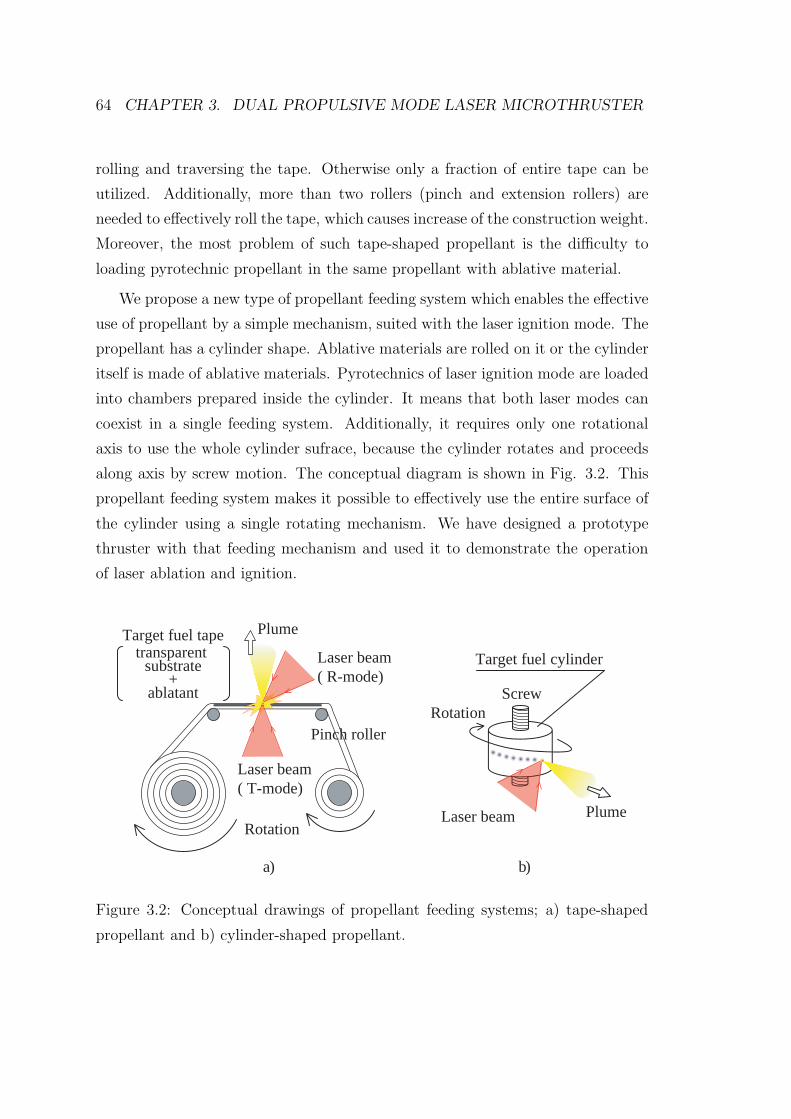
64 CHAPTER 3. DUAL PROPULSIVE MODE LASER MICROTHRUSTER
rolling and traversing the tape. Otherwise only a fraction of entire tape can be
utilized. Additionally, more than two rollers (pinch and extension rollers) are
needed to effectively roll the tape, which causes increase of the construction weight.
Moreover, the most problem of such tape-shaped propellant is the difficulty to
loading pyrotechnic propellant in the same propellant with ablative material.
We propose a new type of propellant feeding system which enables the effective
use of propellant by a simple mechanism, suited with the laser ignition mode. The
propellant has a cylinder shape. Ablative materials are rolled on it or the cylinder
itself is made of ablative materials. Pyrotechnics of laser ignition mode are loaded
into chambers prepared inside the cylinder. It means that both laser modes can
coexist in a single feeding system. Additionally, it requires only one rotational
axis to use the whole cylinder sufrace, because the cylinder rotates and proceeds
along axis by screw motion. The conceptual diagram is shown in Fig. 3.2. This
propellant feeding system makes it possible to effectively use the entire surface of
the cylinder using a single rotating mechanism. We have designed a prototype
thruster with that feeding mechanism and used it to demonstrate the operation
of laser ablation and ignition.
Laser beam( T-mode)
Plume
Pinch roller
Rotation
Target fuel tapetransparent
substrate+
ablatant
Laser beam( R-mode)
Laser beam Plume
Target fuel cylinder
ScrewRotation
a) b)
Figure 3.2: Conceptual drawings of propellant feeding systems; a) tape-shaped
propellant and b) cylinder-shaped propellant.
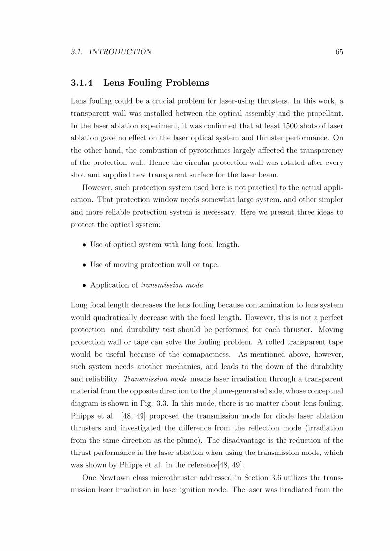
3.1. INTRODUCTION 65
3.1.4 Lens Fouling Problems
Lens fouling could be a crucial problem for laser-using thrusters. In this work, a
transparent wall was installed between the optical assembly and the propellant.
In the laser ablation experiment, it was confirmed that at least 1500 shots of laser
ablation gave no effect on the laser optical system and thruster performance. On
the other hand, the combustion of pyrotechnics largely affected the transparency
of the protection wall. Hence the circular protection wall was rotated after every
shot and supplied new transparent surface for the laser beam.
However, such protection system used here is not practical to the actual appli-
cation. That protection window needs somewhat large system, and other simpler
and more reliable protection system is necessary. Here we present three ideas to
protect the optical system:
• Use of optical system with long focal length.
• Use of moving protection wall or tape.
• Application of transmission mode
Long focal length decreases the lens fouling because contamination to lens system
would quadratically decrease with the focal length. However, this is not a perfect
protection, and durability test should be performed for each thruster. Moving
protection wall or tape can solve the fouling problem. A rolled transparent tape
would be useful because of the comapactness. As mentioned above, however,
such system needs another mechanics, and leads to the down of the durability
and reliability. Transmission mode means laser irradiation through a transparent
material from the opposite direction to the plume-generated side, whose conceptual
diagram is shown in Fig. 3.3. In this mode, there is no matter about lens fouling.
Phipps et al. [48, 49] proposed the transmission mode for diode laser ablation
thrusters and investigated the difference from the reflection mode (irradiation
from the same direction as the plume). The disadvantage is the reduction of the
thrust performance in the laser ablation when using the transmission mode, which
was shown by Phipps et al. in the reference[48, 49].
One Newtown class microthruster addressed in Section 3.6 utilizes the trans-
mission laser irradiation in laser ignition mode. The laser was irradiated from the
66 CHAPTER 3. DUAL PROPULSIVE MODE LASER MICROTHRUSTER
axis toward the outward in radial. Figure 3.3 is an illustration of an application
of transmission mode for laser ablation and ignition.
Diode laser
Ablation plume
Ablation material
Transparent material
Combustion plume
Incident windowPyrotechnics
Nozzle
Diode laserDiode laser
Ablation plume
Ablation material
Transparent material
Combustion plume
Incident windowPyrotechnics
Nozzle
Diode laser
Figure 3.3: Conceptual drawings of transmission modes for laser ablation and
ignition.
3.1.5 Objectives of this chapter
The objectives of this chapter are verifying the operation and clarifying the funda-
mental characteristics of a dual propulsive mode laser microthruster. The charac-
teristics of above-mentioned laser ablation and laser ignition modes are separately
investigated. Both modes use the same propellant feeding system and can be
interchanged by the variety of the propellant, polymer or pyrotechnic.
Laser ablation mode
A number of studies have been conducted in the field of laser ablation. They are
commonly not for the laser ablative propulsion but for various industrial applica-
tions, laser machining, laser hardening, laser deposition and so on. Then physical
processes included in the laser ablation have been well studied [62, 63, 64, 65, 66,
67]. The processes include absorption of laser irradiation, heating the ablative
material by the energy, and the phase transformations. However, there are a few
studies on the characteristics unique on propulsions (thrust and Isp) and those
dependence on the laser parameters. Moreover, most studies on the laser ablation
are using high intensity lasers (CO2, excimer, and YAG) and with extremely short
pulse. The typical laser intensity is over 108 W/m2 and the laser pulse width is less
than 10−6 s in many researches. In contrast, laser beam dealt here is an infrared
3.1. INTRODUCTION 67
laser with lower laser intensity (1 MW/m2) and longer pulse width (100 ms). The
laser ablation physics of those levels has not been focused in this field.
Therefore in this study, first the ablative materials are selected to generate
ablative plume using a diode laser. As a result polyvinyl chloride is considered
as the best material and the fundamental thruster performances: plume direc-
tion, momentum coupling coefficient, specific impulse, and multiple shots effect
are measured with changing the laser pulse width. Next, to clarify the ablation
mechanism, effect of doped carbon density and mass spectroscopy of the exhausted
plume are investigated. In the discussion, photothermal ablation model is applied
in the diode laser ablation processes. It consists of thermal heating and ablating
processes. Analytical expressions are derived and compared with the experimen-
tally measured results.
Laser ignition mode
Several researchers have studied on the laser ignition of chemical propellants [68,
69, 70, 71, 72, 73]. The ignition using laser benefits from the high intensity and
the electrical insulation. They observed that the ignition depends on a thermal
mechanism, and the incident laser energy and the laser power density control the
ignition threshold. They also noticed that the laser energy required for the ignition
decreases as the laser power is increased. However, most of them have conducted
the experiments in the atmosphere. Only a few studies were carried out in the
lower background pressure [70]. Additionally, different kind of lasers, focusing,
and pyrotechnics were used in those studies.
The objectives are first to verify the laser ignition of pyrotechnic in vacuum,
secondly to measure the thrust provided by the combustion, and thirdly to clarify
the required laser conditions for the ignition. In the experiment, after examin-
ing several pyrotechnics, only boron/potassium nitrate succeeds to be ignited in
vacuum. The laser ignition characteristics are investigated against by laser pulse
width and laser power. The obtained threshold laser parameters should be ade-
quate to coexist with laser ablation mode to veryfy the concept of a dual propulsive
mode. Thereafter the thrust measurement is performed. In the discussions, the
reason why boron/potassium nitrate is adequate to the laser ignition in vacuum is
considered. It is shown that the measured threshold laser power and period for the
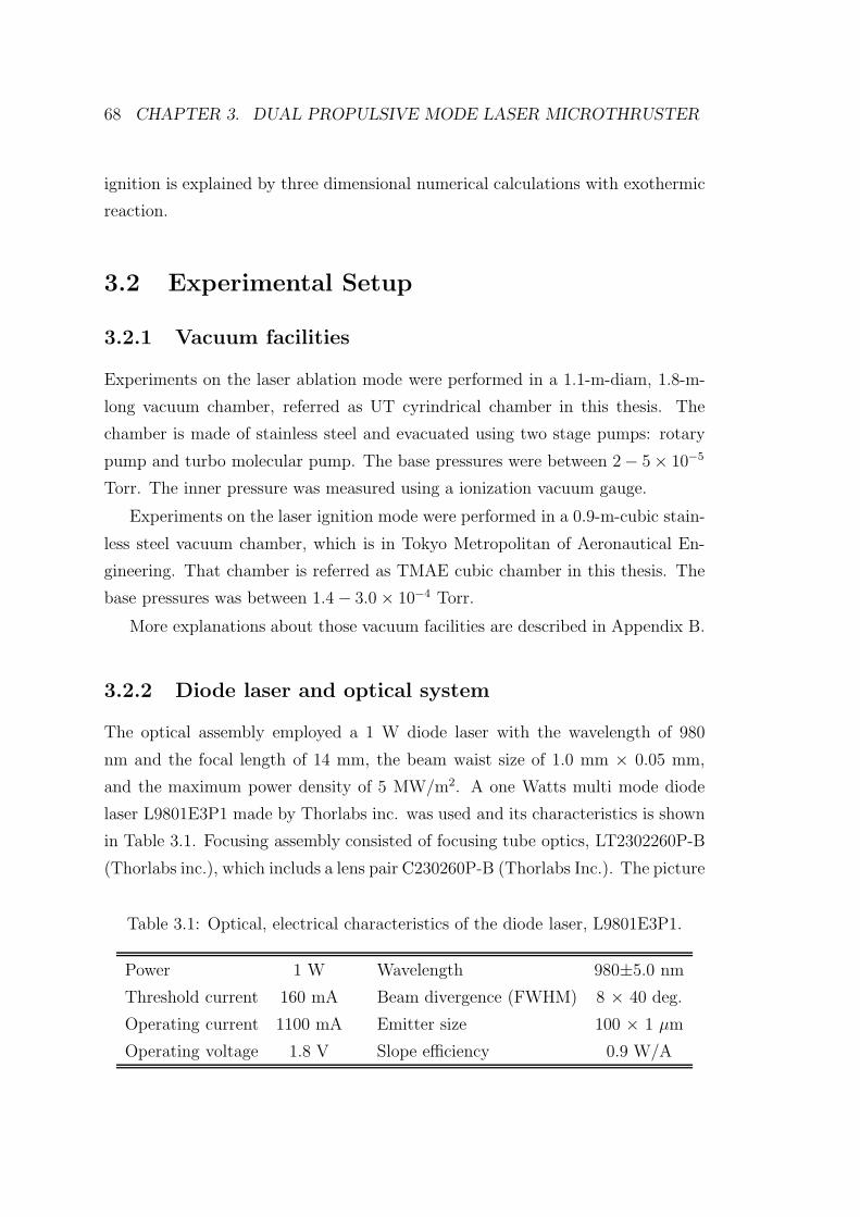
68 CHAPTER 3. DUAL PROPULSIVE MODE LASER MICROTHRUSTER
ignition is explained by three dimensional numerical calculations with exothermic
reaction.
3.2 Experimental Setup
3.2.1 Vacuum facilities
Experiments on the laser ablation mode were performed in a 1.1-m-diam, 1.8-m-
long vacuum chamber, referred as UT cyrindrical chamber in this thesis. The
chamber is made of stainless steel and evacuated using two stage pumps: rotary
pump and turbo molecular pump. The base pressures were between 2 − 5 × 10⁻⁵
Torr. The inner pressure was measured using a ionization vacuum gauge.
Experiments on the laser ignition mode were performed in a 0.9-m-cubic stain-
less steel vacuum chamber, which is in Tokyo Metropolitan of Aeronautical En-
gineering. That chamber is referred as TMAE cubic chamber in this thesis. The
base pressures was between 1.4 − 3.0 × 10⁻⁴ Torr.
More explanations about those vacuum facilities are described in Appendix B.
3.2.2 Diode laser and optical system
The optical assembly employed a 1 W diode laser with the wavelength of 980
nm and the focal length of 14 mm, the beam waist size of 1.0 mm × 0.05 mm,
and the maximum power density of 5 MW/m2. A one Watts multi mode diode
laser L9801E3P1 made by Thorlabs inc. was used and its characteristics is shown
in Table 3.1. Focusing assembly consisted of focusing tube optics, LT2302260P-B
(Thorlabs inc.), which includs a lens pair C230260P-B (Thorlabs Inc.). The picture
Table 3.1: Optical, electrical characteristics of the diode laser, L9801E3P1.
Power 1 W Wavelength 980±5.0 nm
Threshold current 160 mA Beam divergence (FWHM) 8 × 40 deg.
Operating current 1100 mA Emitter size 100 × 1 µm
Operating voltage 1.8 V Slope efficiency 0.9 W/A
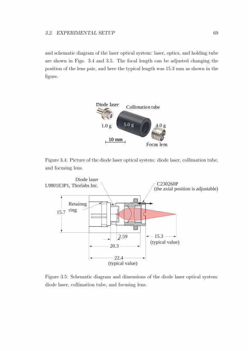
3.2. EXPERIMENTAL SETUP 69
and schematic diagram of the laser optical system: laser, optics, and holding tube
are shown in Figs. 3.4 and 3.5. The focal length can be adjusted changing the
position of the lens pair, and here the typical length was 15.3 mm as shown in the
figure.
10 mm
1.0 g 5.0 g 4.0 g
Focus lens
Diode laser Collimation tube
10 mm10 mm
1.0 g 5.0 g 4.0 g
Focus lens
Diode laser Collimation tube
Figure 3.4: Picture of the diode laser optical system: diode laser, collimation tube,
and focusing lens.
Diode laserL9801E3P1, Thorlabs Inc.
Retainng ring15.7
20.3
2.59
C230260P
15.3
22.4(typical value)
(typical value)
(the axial position is adjustable)
Figure 3.5: Schematic diagram and dimensions of the diode laser optical system:
diode laser, collimation tube, and focusing lens.
70 CHAPTER 3. DUAL PROPULSIVE MODE LASER MICROTHRUSTER
3.2.3 Laser diode driver
Two varieties of laser diode drivers are used to drive the diode laser. In the ex-
periments on the laser ablation mode, WLD3343 made by Wavelength Electronics
Inc. was used. It can supply laser diode current up to 2 A from a single +5 V
power supply and operate with constant current mode or constant power mode.
The output current and the operation mode were selected by the external connec-
tions. The laser pulse width is controlled by TLT signal from a controlling PC.
The output current from the driver dealt here had a lot of high frequency ripples
with DC current. However, the ripples were neglected and the driver was used to
perform the experiment, because the laser pulse width was more than 50 ms and
much lower than the frequency of those ripples. The laser beam power emitted
from the diode laser was about 300 mW, which was measured using a power meter
(LM-10 from Coherent Inc.).
In the early stage of the experiments on the laser ignition mode, the same laser
driver as the laser ablation mode was used. Thereafter, another diode laser driver,
LP3000 made by Thorlabs inc. was used. The laser pulse width was determined by
a controlling PC as well as the laser ablation mode. The diode laser was operated
with the beam power ranged from 300 to 1000 mW.
3.2.4 Beam profile of diode laser
Beam profile from the diode laser was taken using a CCD beam profiler. Generally
laser beam emitted from a diode laser has astigmatic elliptical wavefront profile,
because the lasing cavity has rectangular configuration with high aspect ratio (the
diode laser used here had the emitting size of 100×1 µm). Figure 3.6 is a drawing
of typical diode laser beam. The beam has larger divergence angle perpendicular to
the emitting stripe of diode laser than the angle parallel to it. Then the wavefront
of the laser becomes elliptic as shown the figure. In this study, the perpendicular
and parallel axes are refrred as vertical and horizontal axes.
In order to evaluate the effect of laser intensity on the laser ablation perfor-
mance, beam profile of such elliptical laser beam should be measured. The beam
profiler used here is Beam Star-V from Ophir Optronics Ltd., and its character-
istics is shown in Table 3.2. The beam profiler was set in front of the laser diode
system on a linear sage. By changing the position of the laser diode against the
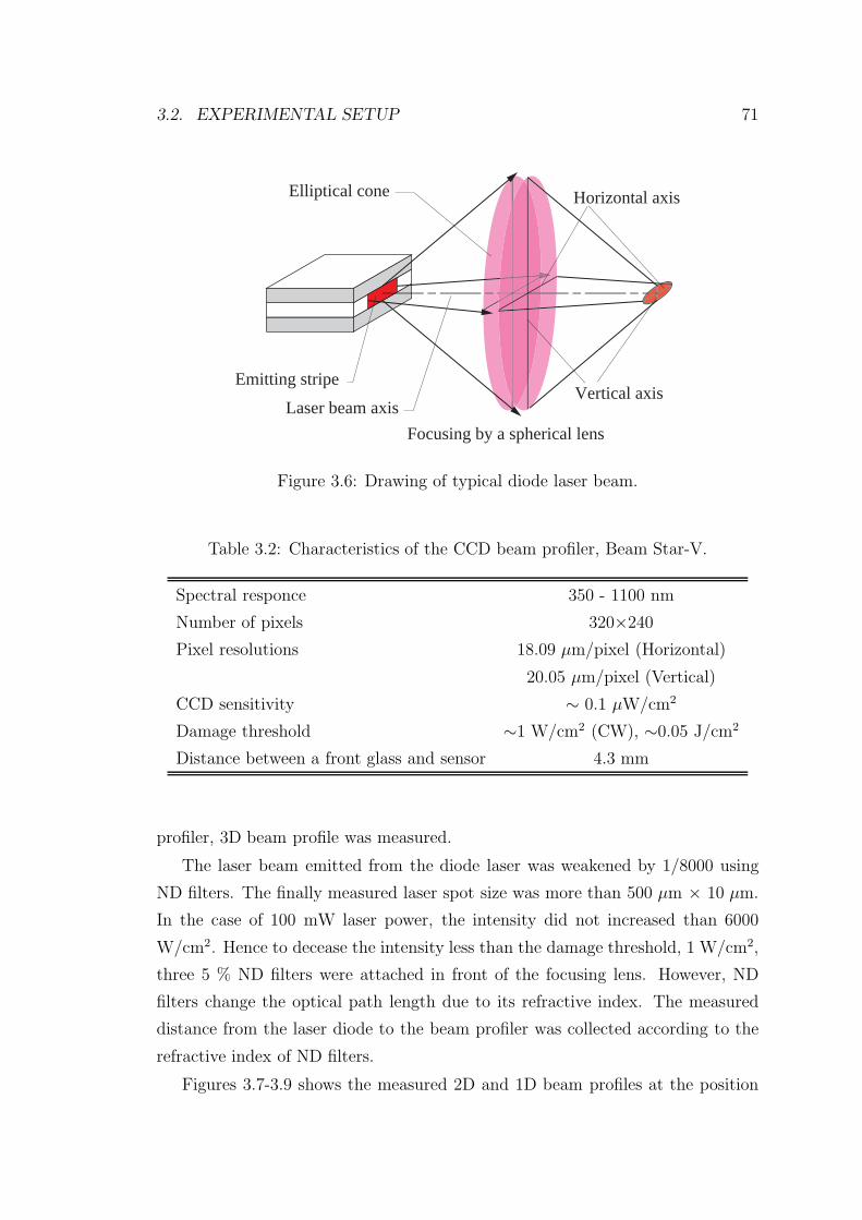
3.2. EXPERIMENTAL SETUP 71
Vertical axis
Horizontal axis
Emitting stripe
Elliptical cone
Focusing by a spherical lensLaser beam axis
Figure 3.6: Drawing of typical diode laser beam.
Table 3.2: Characteristics of the CCD beam profiler, Beam Star-V.
Spectral responce 350 - 1100 nm
Number of pixels 320×240
Pixel resolutions 18.09 µm/pixel (Horizontal)
20.05 µm/pixel (Vertical)
CCD sensitivity ∼ 0.1 µW/cm2
Damage threshold ∼1 W/cm2 (CW), ∼0.05 J/cm2
Distance between a front glass and sensor 4.3 mm
profiler, 3D beam profile was measured.
The laser beam emitted from the diode laser was weakened by 1/8000 using
ND filters. The finally measured laser spot size was more than 500 µm × 10 µm.
In the case of 100 mW laser power, the intensity did not increased than 6000
W/cm2. Hence to decease the intensity less than the damage threshold, 1 W/cm2,
three 5 % ND filters were attached in front of the focusing lens. However, ND
filters change the optical path length due to its refractive index. The measured
distance from the laser diode to the beam profiler was collected according to the
refractive index of ND filters.
Figures 3.7-3.9 shows the measured 2D and 1D beam profiles at the position
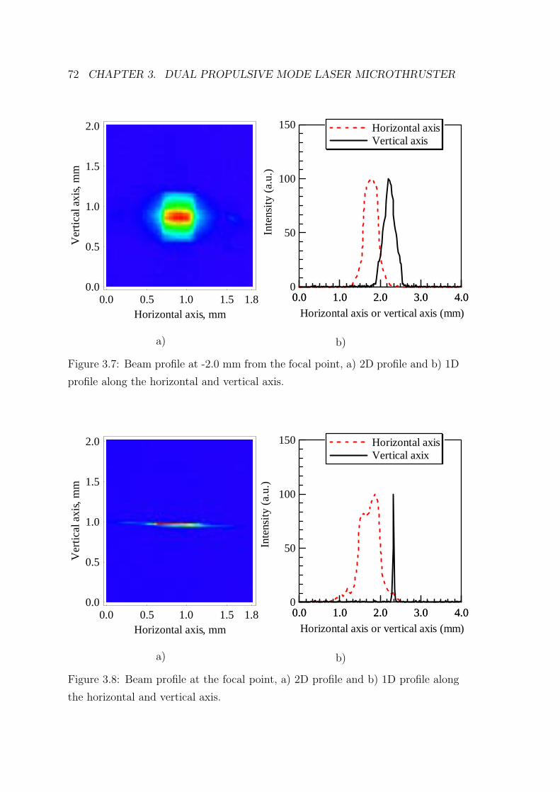
72 CHAPTER 3. DUAL PROPULSIVE MODE LASER MICROTHRUSTER
0.0 0.5 1.0 1.5 1.8Horizontal axis, mm
0.0
0.5
1.0
1.5
2.0
Ver
tical
axis
,mm
a)
150
100
50
0
Inte
nsit
y (a
.u.)
4.03.02.01.00.0
Horizontal axis or vertical axis (mm)
4.03.02.01.00.0
Horizontal axis Vertical axis
b)
Figure 3.7: Beam profile at -2.0 mm from the focal point, a) 2D profile and b) 1D
profile along the horizontal and vertical axis.
0.0 0.5 1.0 1.5 1.8Horizontal axis, mm
0.0
0.5
1.0
1.5
2.0
Ver
tical
axis
,mm
a)
150
100
50
0
Inte
nsit
y (a
.u.)
4.03.02.01.00.0
Horizontal axis or vertical axis (mm)
4.03.02.01.00.0
Horizontal axis Vertical axix
b)
Figure 3.8: Beam profile at the focal point, a) 2D profile and b) 1D profile along
the horizontal and vertical axis.
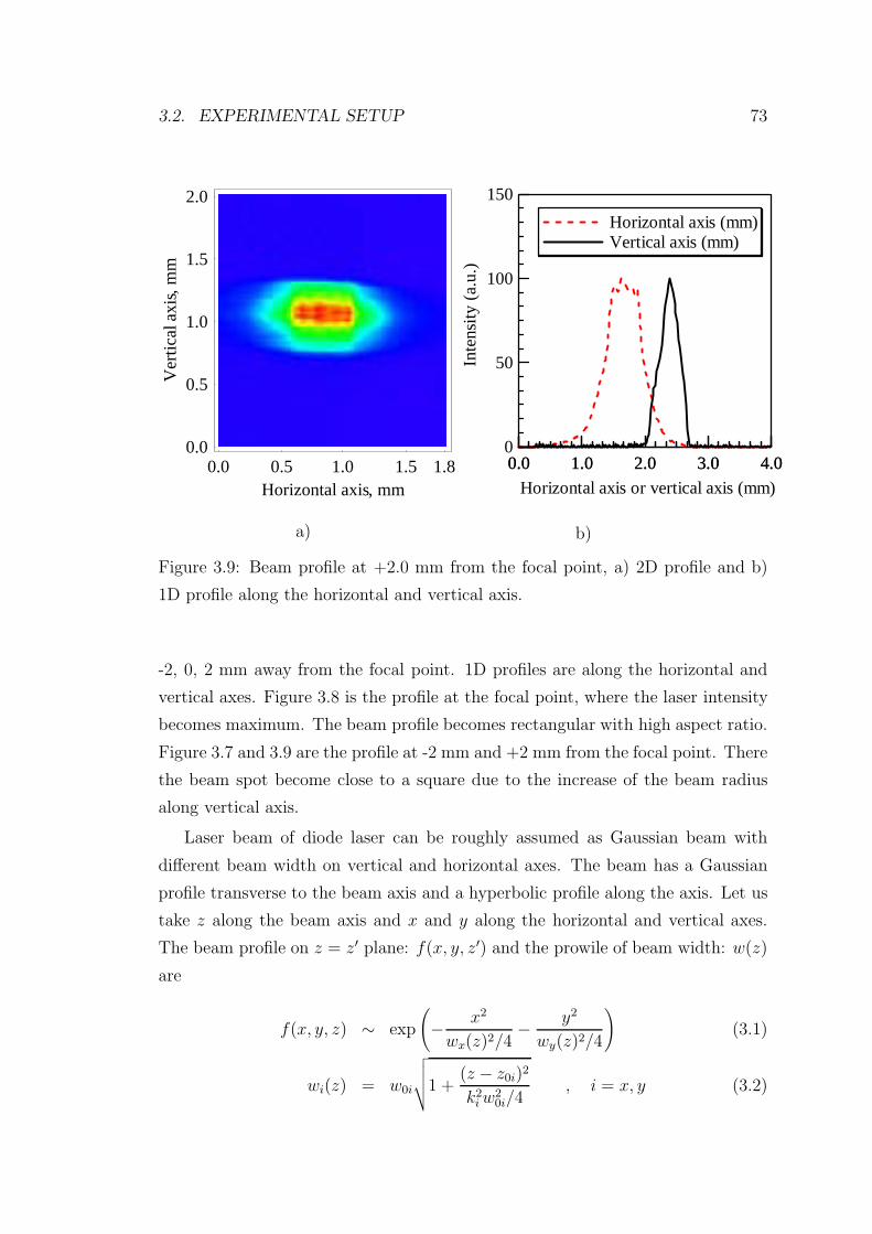
3.2. EXPERIMENTAL SETUP 73
0.0 0.5 1.0 1.5 1.8Horizontal axis, mm
0.0
0.5
1.0
1.5
2.0
Ver
tical
axis
,mm
a)
150
100
50
0In
tens
ity
(a.u
.)4.03.02.01.00.0
Horizontal axis or vertical axis (mm)
4.03.02.01.00.0
Horizontal axis (mm) Vertical axis (mm)
b)
Figure 3.9: Beam profile at +2.0 mm from the focal point, a) 2D profile and b)
1D profile along the horizontal and vertical axis.
-2, 0, 2 mm away from the focal point. 1D profiles are along the horizontal and
vertical axes. Figure 3.8 is the profile at the focal point, where the laser intensity
becomes maximum. The beam profile becomes rectangular with high aspect ratio.
Figure 3.7 and 3.9 are the profile at -2 mm and +2 mm from the focal point. There
the beam spot become close to a square due to the increase of the beam radius
along vertical axis.
Laser beam of diode laser can be roughly assumed as Gaussian beam with
different beam width on vertical and horizontal axes. The beam has a Gaussian
profile transverse to the beam axis and a hyperbolic profile along the axis. Let us
take z along the beam axis and x and y along the horizontal and vertical axes.
The beam profile on z = z′ plane: f(x, y, z′) and the prowile of beam width: w(z)
are
f(x, y, z) ∼ exp
(− x2
wx(z)2/4− y2
wy(z)2/4
)(3.1)
wi(z) = w0i
√√√√1 +(z − z0i)2
k2i w
20i/4
, i = x, y (3.2)
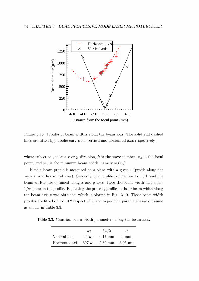
74 CHAPTER 3. DUAL PROPULSIVE MODE LASER MICROTHRUSTER
1250
1000
750
500
250
0
Bea
m d
iam
eter
(µm
)
-6.0 -4.0 -2.0 0.0 2.0 4.0
Distance from the focul point (mm)
-6.0 -4.0 -2.0 0.0 2.0 4.0
Horizontal axis Vertical axis
Figure 3.10: Profiles of beam widths along the beam axis. The solid and dashed
lines are fitted hyperbolic curves for vertical and horizontal axis respectively.
where subscript i means x or y direction, k is the wave number, z0i is the focul
point, and w0i is the minimum beam width, namely wi(z0i).
First a beam profile is measured on a plane with a given z (profile along the
vertical and horizontal axes). Secondly, that profile is fitted on Eq. 3.1, and the
beam widths are obtained along x and y axes. Here the beam width means the
1/e2 point in the profile. Repeating the process, profiles of laser beam width along
the beam axis z was obtained, which is plotted in Fig. 3.10. Those beam width
profiles are fitted on Eq. 3.2 respectively, and hyperbolic parameters are obtained
as shown in Table 3.3.
Table 3.3: Gaussian beam width parameters along the beam axis.
ω0 kω/2 z0
Vertical axis 46 µm 0.17 mm 0 mm
Horizontal axis 607 µm 2.89 mm -3.05 mm
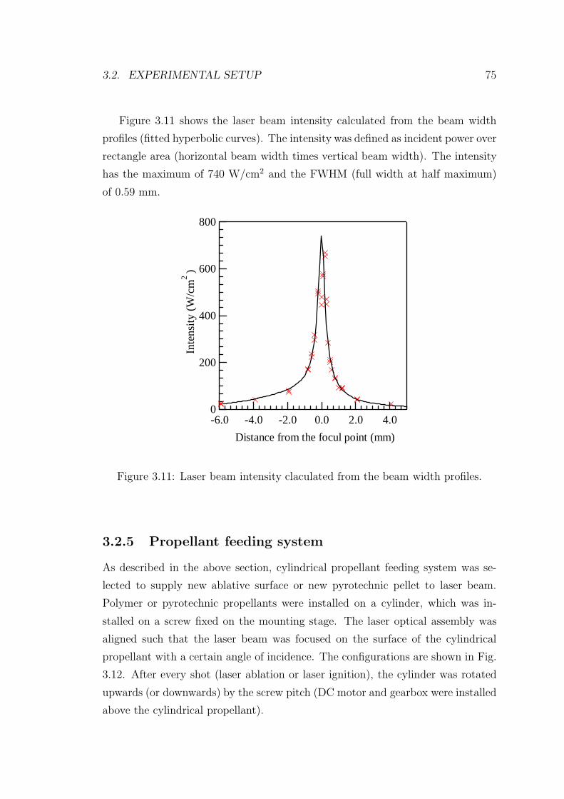
3.2. EXPERIMENTAL SETUP 75
Figure 3.11 shows the laser beam intensity calculated from the beam width
profiles (fitted hyperbolic curves). The intensity was defined as incident power over
rectangle area (horizontal beam width times vertical beam width). The intensity
has the maximum of 740 W/cm2 and the FWHM (full width at half maximum)
of 0.59 mm.
800
600
400
200
0
Inte
nsit
y (W
/cm
2 )
-6.0 -4.0 -2.0 0.0 2.0 4.0
Distance from the focul point (mm)
Figure 3.11: Laser beam intensity claculated from the beam width profiles.
3.2.5 Propellant feeding system
As described in the above section, cylindrical propellant feeding system was se-
lected to supply new ablative surface or new pyrotechnic pellet to laser beam.
Polymer or pyrotechnic propellants were installed on a cylinder, which was in-
stalled on a screw fixed on the mounting stage. The laser optical assembly was
aligned such that the laser beam was focused on the surface of the cylindrical
propellant with a certain angle of incidence. The configurations are shown in Fig.
3.12. After every shot (laser ablation or laser ignition), the cylinder was rotated
upwards (or downwards) by the screw pitch (DC motor and gearbox were installed
above the cylindrical propellant).
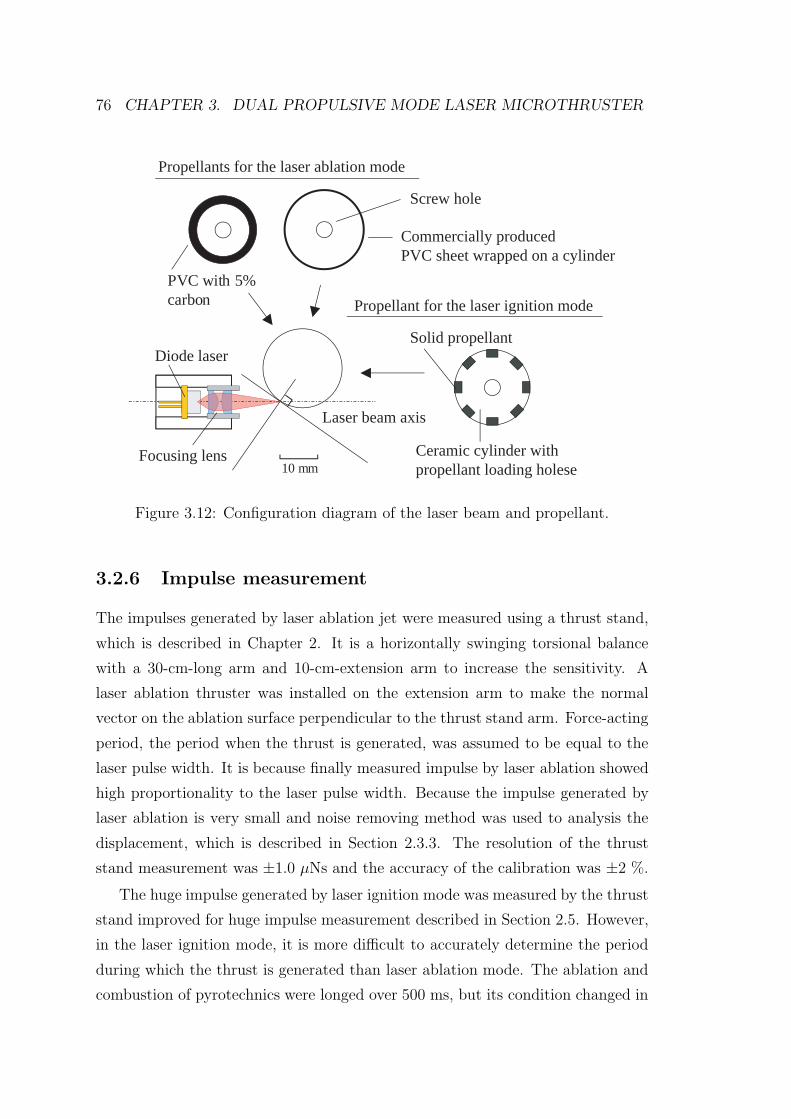
76 CHAPTER 3. DUAL PROPULSIVE MODE LASER MICROTHRUSTER
Commercially produced PVC sheet wrapped on a cylinder
Propellant for the laser ignition mode
Diode laser
Laser beam axis
PVC with 5% carbon
Focusing lens
Propellants for the laser ablation mode
Solid propellant
Screw hole
Ceramic cylinder with propellant loading holese10 mm
Figure 3.12: Configuration diagram of the laser beam and propellant.
3.2.6 Impulse measurement
The impulses generated by laser ablation jet were measured using a thrust stand,
which is described in Chapter 2. It is a horizontally swinging torsional balance
with a 30-cm-long arm and 10-cm-extension arm to increase the sensitivity. A
laser ablation thruster was installed on the extension arm to make the normal
vector on the ablation surface perpendicular to the thrust stand arm. Force-acting
period, the period when the thrust is generated, was assumed to be equal to the
laser pulse width. It is because finally measured impulse by laser ablation showed
high proportionality to the laser pulse width. Because the impulse generated by
laser ablation is very small and noise removing method was used to analysis the
displacement, which is described in Section 2.3.3. The resolution of the thrust
stand measurement was ±1.0 µNs and the accuracy of the calibration was ±2 %.
The huge impulse generated by laser ignition mode was measured by the thrust
stand improved for huge impulse measurement described in Section 2.5. However,
in the laser ignition mode, it is more difficult to accurately determine the period
during which the thrust is generated than laser ablation mode. The ablation and
combustion of pyrotechnics were longed over 500 ms, but its condition changed in
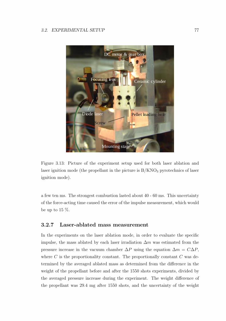
3.2. EXPERIMENTAL SETUP 77
Mounting stage
ScrewScrew
Pellet loading holePellet loading hole
DC motor & gear box
Diode laser
Focusing lens Ceramic cylinder
Mounting stage
ScrewScrew
Pellet loading holePellet loading hole
DC motor & gear box
Diode laser
Focusing lens Ceramic cylinder
Figure 3.13: Picture of the experiment setup used for both laser ablation and
laser ignition mode (the propellant in the picture is B/KNO3 pyrotechnics of laser
ignition mode).
a few ten ms. The strongest combustion lasted about 40 - 60 ms. This uncertainty
of the force-acting time caused the error of the impulse measurement, which would
be up to 15 %.
3.2.7 Laser-ablated mass measurement
In the experiments on the laser ablation mode, in order to evaluate the specific
impulse, the mass ablated by each laser irradiation ∆m was estimated from the
pressure increase in the vacuum chamber ∆P using the equation ∆m = C∆P ,
where C is the proportionality constant. The proportionally constant C was de-
termined by the averaged ablated mass as determined from the difference in the
weight of the propellant before and after the 1550 shots experiments, divided by
the averaged pressure increase during the experiment. The weight difference of
the propellant was 29.4 mg after 1550 shots, and the uncertainty of the weight
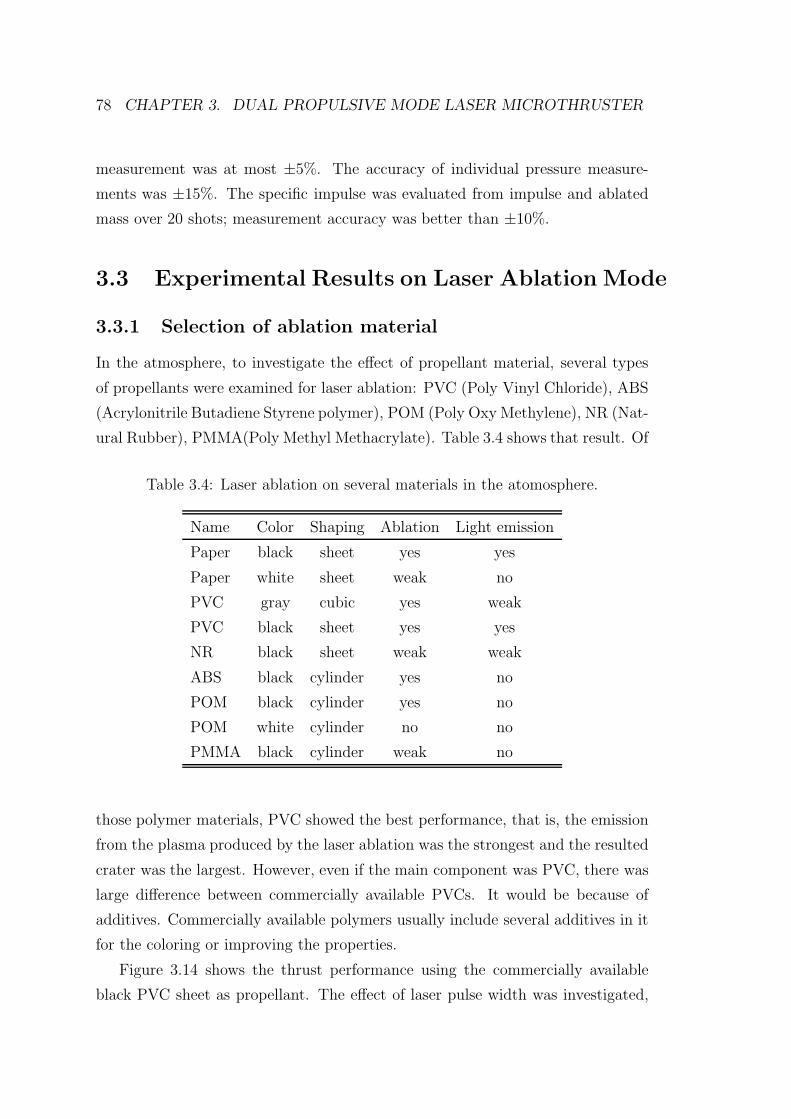
78 CHAPTER 3. DUAL PROPULSIVE MODE LASER MICROTHRUSTER
measurement was at most ±5%. The accuracy of individual pressure measure-
ments was ±15%. The specific impulse was evaluated from impulse and ablated
mass over 20 shots; measurement accuracy was better than ±10%.
3.3 Experimental Results on Laser Ablation Mode
3.3.1 Selection of ablation material
In the atmosphere, to investigate the effect of propellant material, several types
of propellants were examined for laser ablation: PVC (Poly Vinyl Chloride), ABS
(Acrylonitrile Butadiene Styrene polymer), POM (Poly Oxy Methylene), NR (Nat-
ural Rubber), PMMA(Poly Methyl Methacrylate). Table 3.4 shows that result. Of
Table 3.4: Laser ablation on several materials in the atomosphere.
Name Color Shaping Ablation Light emission
Paper black sheet yes yes
Paper white sheet weak no
PVC gray cubic yes weak
PVC black sheet yes yes
NR black sheet weak weak
ABS black cylinder yes no
POM black cylinder yes no
POM white cylinder no no
PMMA black cylinder weak no
those polymer materials, PVC showed the best performance, that is, the emission
from the plasma produced by the laser ablation was the strongest and the resulted
crater was the largest. However, even if the main component was PVC, there was
large difference between commercially available PVCs. It would be because of
additives. Commercially available polymers usually include several additives in it
for the coloring or improving the properties.
Figure 3.14 shows the thrust performance using the commercially available
black PVC sheet as propellant. The effect of laser pulse width was investigated,
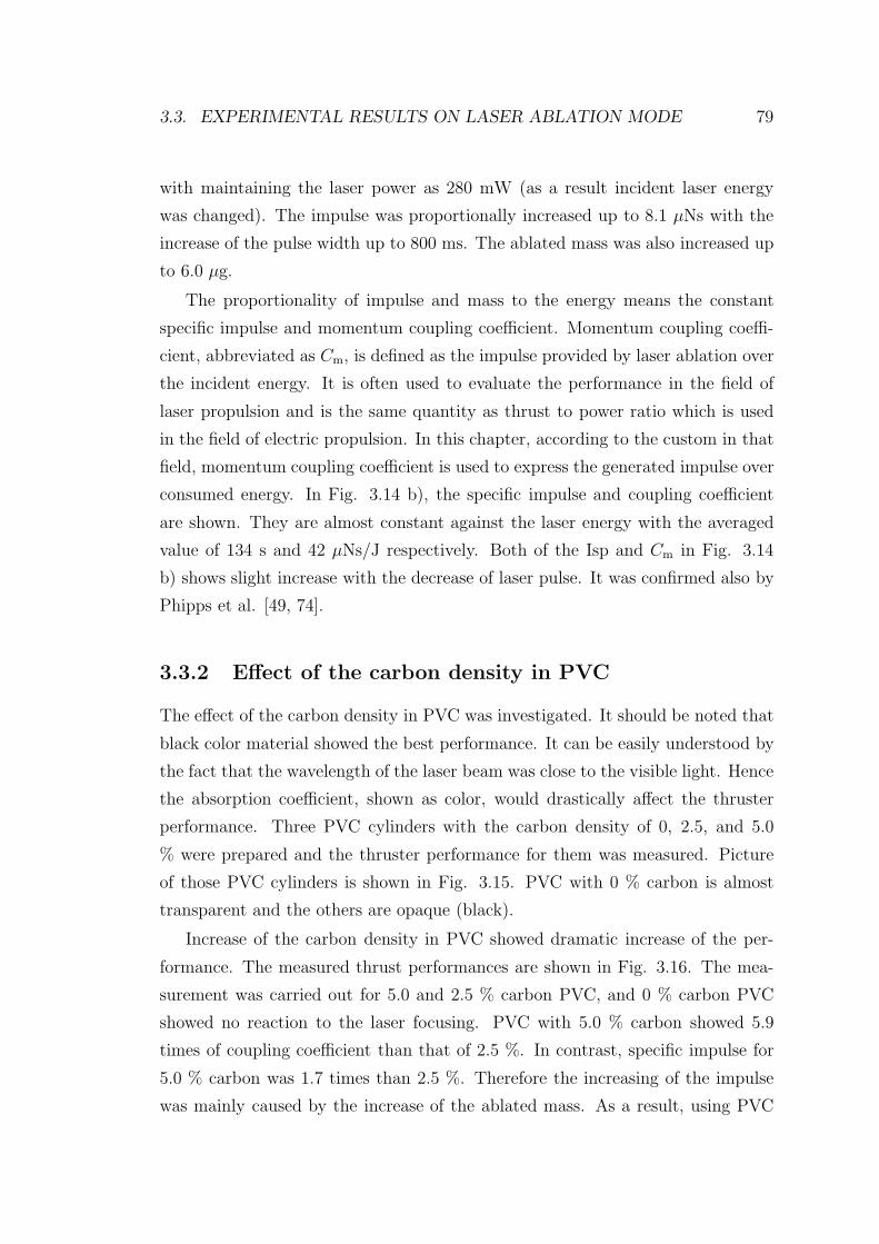
3.3. EXPERIMENTAL RESULTS ON LASER ABLATION MODE 79
with maintaining the laser power as 280 mW (as a result incident laser energy
was changed). The impulse was proportionally increased up to 8.1 µNs with the
increase of the pulse width up to 800 ms. The ablated mass was also increased up
to 6.0 µg.
The proportionality of impulse and mass to the energy means the constant
specific impulse and momentum coupling coefficient. Momentum coupling coeffi-
cient, abbreviated as Cm, is defined as the impulse provided by laser ablation over
the incident energy. It is often used to evaluate the performance in the field of
laser propulsion and is the same quantity as thrust to power ratio which is used
in the field of electric propulsion. In this chapter, according to the custom in that
field, momentum coupling coefficient is used to express the generated impulse over
consumed energy. In Fig. 3.14 b), the specific impulse and coupling coefficient
are shown. They are almost constant against the laser energy with the averaged
value of 134 s and 42 µNs/J respectively. Both of the Isp and Cm in Fig. 3.14
b) shows slight increase with the decrease of laser pulse. It was confirmed also by
Phipps et al. [49, 74].
3.3.2 Effect of the carbon density in PVC
The effect of the carbon density in PVC was investigated. It should be noted that
black color material showed the best performance. It can be easily understood by
the fact that the wavelength of the laser beam was close to the visible light. Hence
the absorption coefficient, shown as color, would drastically affect the thruster
performance. Three PVC cylinders with the carbon density of 0, 2.5, and 5.0
% were prepared and the thruster performance for them was measured. Picture
of those PVC cylinders is shown in Fig. 3.15. PVC with 0 % carbon is almost
transparent and the others are opaque (black).
Increase of the carbon density in PVC showed dramatic increase of the per-
formance. The measured thrust performances are shown in Fig. 3.16. The mea-
surement was carried out for 5.0 and 2.5 % carbon PVC, and 0 % carbon PVC
showed no reaction to the laser focusing. PVC with 5.0 % carbon showed 5.9
times of coupling coefficient than that of 2.5 %. In contrast, specific impulse for
5.0 % carbon was 1.7 times than 2.5 %. Therefore the increasing of the impulse
was mainly caused by the increase of the ablated mass. As a result, using PVC
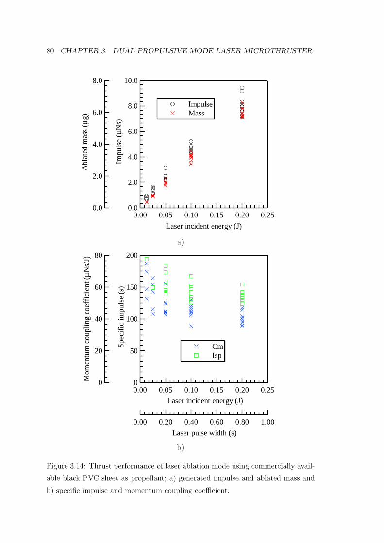
80 CHAPTER 3. DUAL PROPULSIVE MODE LASER MICROTHRUSTER
10.0
8.0
6.0
4.0
2.0
0.0
Impu
lse
(µN
s)
0.250.200.150.100.050.00
Laser incident energy (J)
8.0
6.0
4.0
2.0
0.0
Abl
ated
mas
s (µ
g)
Impulse Mass
a)
80
60
40
20
0Mom
entu
m c
oupl
ing
coef
fici
ent (
µNs/
J)
0.250.200.150.100.050.00
Laser incident energy (J)
200
150
100
50
0
Spe
cifi
c im
puls
e (s
)
1.000.800.600.400.200.00
Laser pulse width (s)
Cm Isp
b)
Figure 3.14: Thrust performance of laser ablation mode using commercially avail-
able black PVC sheet as propellant; a) generated impulse and ablated mass and
b) specific impulse and momentum coupling coefficient.
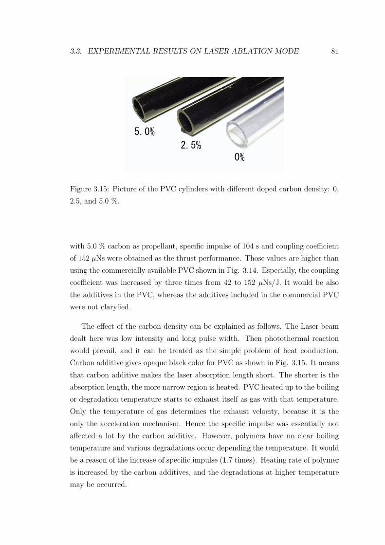
3.3. EXPERIMENTAL RESULTS ON LASER ABLATION MODE 81
Figure 3.15: Picture of the PVC cylinders with different doped carbon density: 0,
2.5, and 5.0 %.
with 5.0 % carbon as propellant, specific impulse of 104 s and coupling coefficient
of 152 µNs were obtained as the thrust performance. Those values are higher than
using the commercially available PVC shown in Fig. 3.14. Especially, the coupling
coefficient was increased by three times from 42 to 152 µNs/J. It would be also
the additives in the PVC, whereas the additives included in the commercial PVC
were not claryfied.
The effect of the carbon density can be explained as follows. The Laser beam
dealt here was low intensity and long pulse width. Then photothermal reaction
would prevail, and it can be treated as the simple problem of heat conduction.
Carbon additive gives opaque black color for PVC as shown in Fig. 3.15. It means
that carbon additive makes the laser absorption length short. The shorter is the
absorption length, the more narrow region is heated. PVC heated up to the boiling
or degradation temperature starts to exhaust itself as gas with that temperature.
Only the temperature of gas determines the exhaust velocity, because it is the
only the acceleration mechanism. Hence the specific impulse was essentially not
affected a lot by the carbon additive. However, polymers have no clear boiling
temperature and various degradations occur depending the temperature. It would
be a reason of the increase of specific impulse (1.7 times). Heating rate of polymer
is increased by the carbon additives, and the degradations at higher temperature
may be occurred.
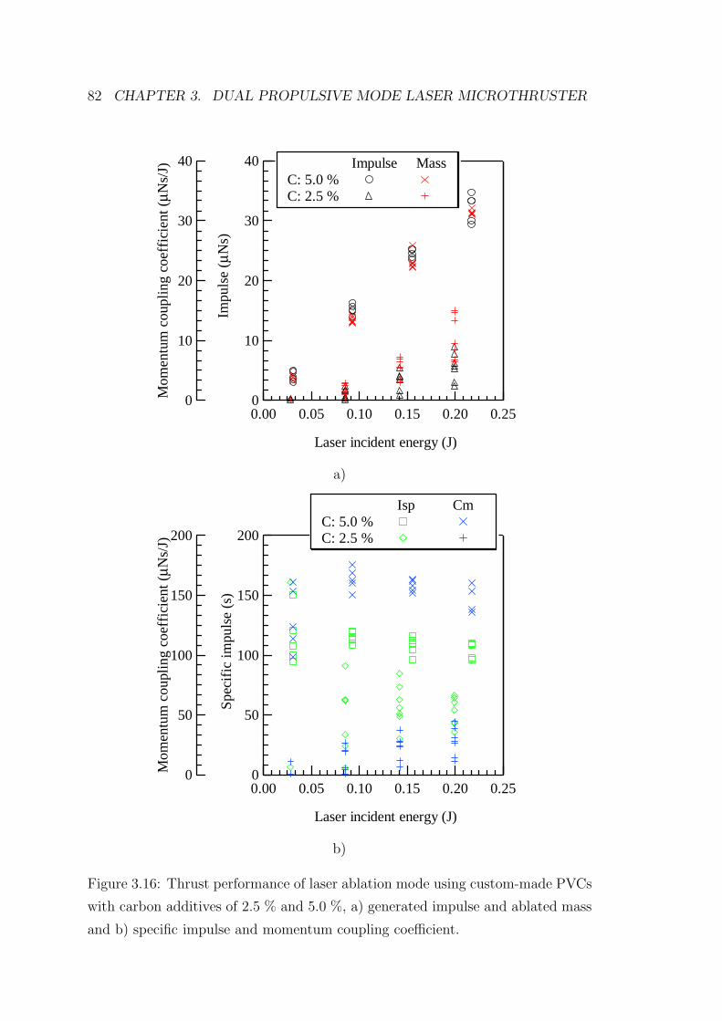
82 CHAPTER 3. DUAL PROPULSIVE MODE LASER MICROTHRUSTER
40
30
20
10
0
Impu
lse
(µN
s)
0.250.200.150.100.050.00
Laser incident energy (J)
40
30
20
10
0Mom
entu
m c
oupl
ing
coef
fici
ent (
µNs/
J) Impulse Mass C: 5.0 % C: 2.5 %
a)
200
150
100
50
0
Spe
cifi
c im
puls
e (s
)
0.250.200.150.100.050.00
Laser incident energy (J)
200
150
100
50
0Mom
entu
m c
oupl
ing
coef
fici
ent (
µNs/
J)
Isp Cm C: 5.0 % C: 2.5 %
b)
Figure 3.16: Thrust performance of laser ablation mode using custom-made PVCs
with carbon additives of 2.5 % and 5.0 %, a) generated impulse and ablated mass
and b) specific impulse and momentum coupling coefficient.
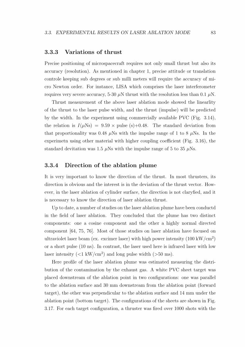
3.3. EXPERIMENTAL RESULTS ON LASER ABLATION MODE 83
3.3.3 Variations of thrust
Precise positioning of microspacecraft requires not only small thrust but also its
accuracy (resolution). As mentioned in chapter 1, precise attitude or translation
controle keeping sub degrees or sub milli meters will require the accuracy of mi-
cro Newton order. For instance, LISA which comprises the laser interferometer
requires very severe accuracy, 5-30 µN thrust with the resolution less than 0.1 µN.
Thrust measurement of the above laser ablation mode showed the linearlity
of the thrust to the laser pulse width, and the thrust (impulse) will be predicted
by the width. In the experiment using commercially available PVC (Fig. 3.14),
the relation is I(µNs) = 9.59 × pulse (s)+0.48. The standard deviation from
that proportionality was 0.48 µNs with the impulse range of 1 to 8 µNs. In the
experimetn using other material with higher coupling coefficient (Fig. 3.16), the
standard devitation was 1.5 µNs with the impulse range of 5 to 35 µNs.
3.3.4 Direction of the ablation plume
It is very important to know the direction of the thrust. In most thrusters, its
direction is obvious and the interest is in the deviation of the thrust vector. How-
ever, in the laser ablation of cylinder surface, the direction is not claryfied, and it
is necessary to know the direction of laser ablation thrust.
Up to date, a number of studies on the laser ablation plume have been conductd
in the field of laser ablation. They concluded that the plume has two distinct
components: one a cosine component and the other a highly normal directed
component [64, 75, 76]. Most of those studies on laser ablation have focused on
ultraviolet laser beam (ex. excimer laser) with high power intensity (100 kW/cm2)
or a short pulse (10 ns). In contrast, the laser used here is infrared laser with low
laser intensity (<1 kW/cm2) and long pulse width (>50 ms).
Here profile of the laser ablation plume was estimated measuring the distri-
bution of the contamination by the exhaust gas. A white PVC sheet target was
placed downstream of the ablation point in two configurations: one was parallel
to the ablation surface and 30 mm downstream from the ablation point (forward
target), the other was perpendicular to the ablation surface and 14 mm under the
ablation point (bottom target). The configurations of the sheets are shown in Fig.
3.17. For each target configuration, a thruster was fired over 1000 shots with the
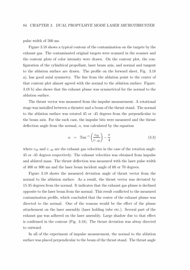
84 CHAPTER 3. DUAL PROPULSIVE MODE LASER MICROTHRUSTER
pulse width of 500 ms.
Figure 3.18 shows a typical contour of the contamination on the targets by the
exhaust gas. The contaminated original targets were scanned in the scanner and
the contour plots of color intensity were drawn. On the contour plot, the con-
figuration of the cylindrical propellant, laser beam axis, and normal and tangent
to the ablation surface are drawn. The profile on the forward sheet, Fig. 3.18
a), has good axial symmetry. The line from the ablation point to the center of
that contour plot almost agreed with the normal to the ablation surface. Figure.
3.18 b) also shows that the exhaust plume was symmetrical for the normal to the
ablation surface.
The thrust vector was measured from the impulse measurement. A rotational
stage was installed between a thruster and a beam of the thrust stand. The normal
to the ablation surface was rotated 45 or -45 degrees from the perpendicular to
the beam axis. For the each case, the impulse bits were measured and the thrust
deflection angle from the normal, α, was calculated by the equation
α = Tan−1
(v45
v−45
)− π
4(3.3)
where v45 and v−45 are the exhaust gas velocities in the case of the rotation angle:
45 or -45 degrees respectively. The exhaust velocities was obtained from impulse
and ablated mass. The thrust deflection was measured with the laser pulse width
of 400 or 800 ms and the laser beam incident angle of 60 or 70 degrees.
Figure 3.19 shows the measured deviation angle of thrust vector from the
normal to the ablation surface. As a result, the thrust vector was deviated by
15-35 degrees from the normal. It indicates that the exhaust gas plume is declined
opposite to the laser beam from the normal. This result conflicted to the measured
contamination profile, which concluded that the center of the exhaust plume was
directed to the normal. One of the reasons would be the effect of the plume
attachement on the laser assembly (laser holding tube etc.). Several part of the
exhaust gas was adhered on the laser assembly. Large shadow due to that effect
is confirmed in the contour (Fig. 3.18). The thrust deviation was alway directed
to outward.
In all of the experiment of impulse measurement, the normal to the ablation
surface was placed perpendicular to the beam of the thrust stand. The thrust angle
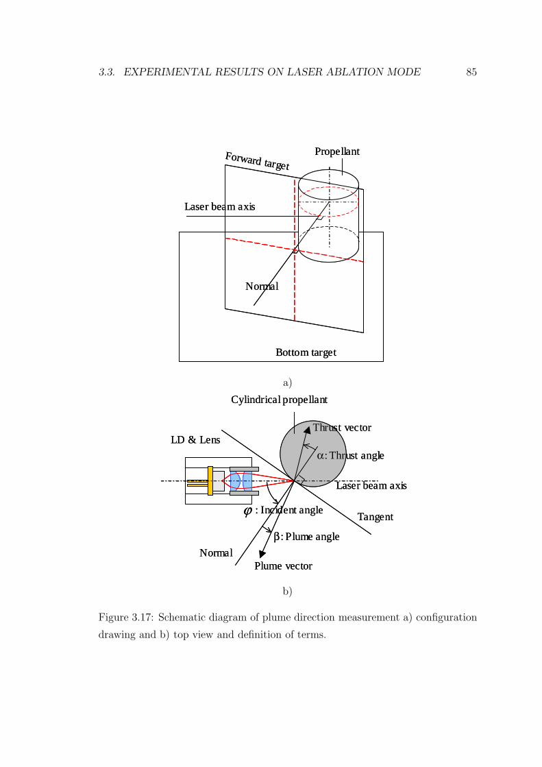
3.3. EXPERIMENTAL RESULTS ON LASER ABLATION MODE 85
Propellant
Laser beam axis
Normal
Forward target
Bottom target
Propellant
Laser beam axis
Normal
Forward target
Bottom target
a)
Cylindrical propellant
LD & Lens
Tangent
Laser beam axis
: Incident angle
β: Plume angle
α: Thrust angle
Thrust vector
Plume vector
ϕ
Normal
Cylindrical propellant
LD & Lens
Tangent
Laser beam axis
: Incident angle
β: Plume angle
α: Thrust angle
Thrust vector
Plume vector
ϕ
Normal
b)
Figure 3.17: Schematic diagram of plume direction measurement a) configuration
drawing and b) top view and definition of terms.
86 CHAPTER 3. DUAL PROPULSIVE MODE LASER MICROTHRUSTER
Shadow of diode laser assembly
Shadow of the stage
Shadow of diode laser assembly
Shadow of the stage
a)
Shadow of diode laser assembly
Laser beam axis
Normal
Tangent
Propellant
Shadow of diode laser assembly
Laser beam axis
Normal
Tangent
Propellant
b)
Figure 3.18: Scanned images contaminated by the exhaust gas: a) forward target
and b) bottom target.
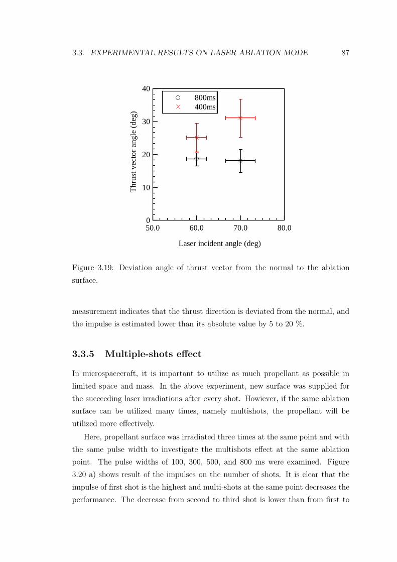
3.3. EXPERIMENTAL RESULTS ON LASER ABLATION MODE 87
40
30
20
10
0
Thr
ust v
ecto
r an
gle
(deg
)
80.070.060.050.0
Laser incident angle (deg)
800ms 400ms
Figure 3.19: Deviation angle of thrust vector from the normal to the ablation
surface.
measurement indicates that the thrust direction is deviated from the normal, and
the impulse is estimated lower than its absolute value by 5 to 20 %.
3.3.5 Multiple-shots effect
In microspacecraft, it is important to utilize as much propellant as possible in
limited space and mass. In the above experiment, new surface was supplied for
the succeeding laser irradiations after every shot. Howiever, if the same ablation
surface can be utilized many times, namely multishots, the propellant will be
utilized more effectively.
Here, propellant surface was irradiated three times at the same point and with
the same pulse width to investigate the multishots effect at the same ablation
point. The pulse widths of 100, 300, 500, and 800 ms were examined. Figure
3.20 a) shows result of the impulses on the number of shots. It is clear that the
impulse of first shot is the highest and multi-shots at the same point decreases the
performance. The decrease from second to third shot is lower than from first to
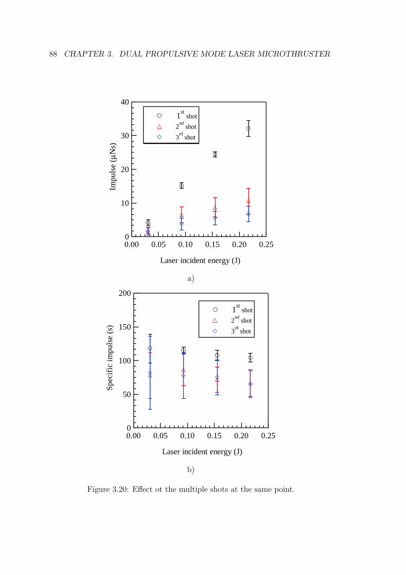
88 CHAPTER 3. DUAL PROPULSIVE MODE LASER MICROTHRUSTER
40
30
20
10
0
Impu
lse
(µN
s)
0.250.200.150.100.050.00
Laser incident energy (J)
1st
shot
2nd
shot
3rd
shot
a)
200
150
100
50
0
Spe
cifi
c im
puls
e (s
)
0.250.200.150.100.050.00
Laser incident energy (J)
1st
shot
2nd
shot
3rd
shot
b)
Figure 3.20: Effect ot the multiple shots at the same point.
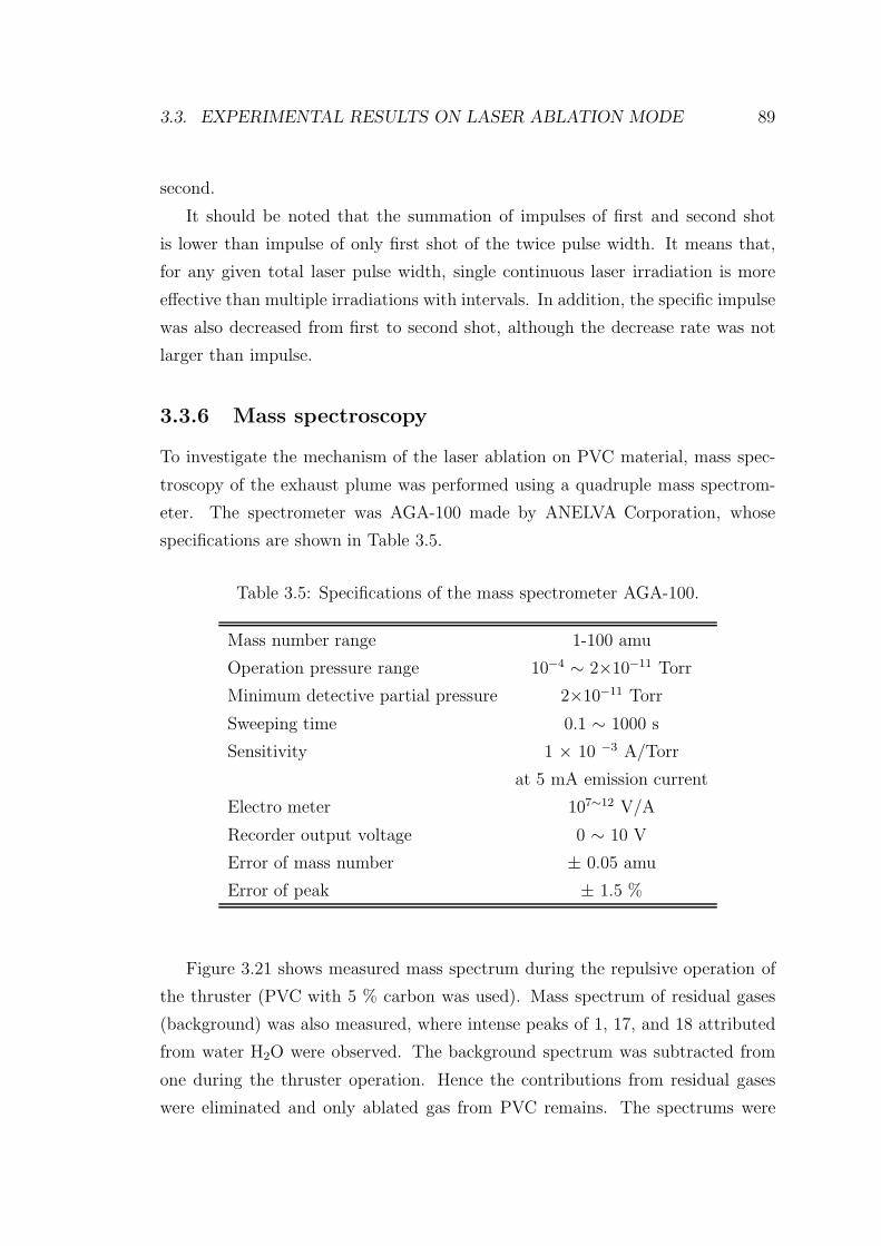
3.3. EXPERIMENTAL RESULTS ON LASER ABLATION MODE 89
second.
It should be noted that the summation of impulses of first and second shot
is lower than impulse of only first shot of the twice pulse width. It means that,
for any given total laser pulse width, single continuous laser irradiation is more
effective than multiple irradiations with intervals. In addition, the specific impulse
was also decreased from first to second shot, although the decrease rate was not
larger than impulse.
3.3.6 Mass spectroscopy
To investigate the mechanism of the laser ablation on PVC material, mass spec-
troscopy of the exhaust plume was performed using a quadruple mass spectrom-
eter. The spectrometer was AGA-100 made by ANELVA Corporation, whose
specifications are shown in Table 3.5.
Table 3.5: Specifications of the mass spectrometer AGA-100.
Mass number range 1-100 amu
Operation pressure range 10−4 ∼ 2×10⁻¹¹ Torr
Minimum detective partial pressure 2×10⁻¹¹ Torr
Sweeping time 0.1 ∼ 1000 s
Sensitivity 1 × 10 −3 A/Torr
at 5 mA emission current
Electro meter 107∼12 V/A
Recorder output voltage 0 ∼ 10 V
Error of mass number ± 0.05 amu
Error of peak ± 1.5 %
Figure 3.21 shows measured mass spectrum during the repulsive operation of
the thruster (PVC with 5 % carbon was used). Mass spectrum of residual gases
(background) was also measured, where intense peaks of 1, 17, and 18 attributed
from water H2O were observed. The background spectrum was subtracted from
one during the thruster operation. Hence the contributions from residual gases
were eliminated and only ablated gas from PVC remains. The spectrums were
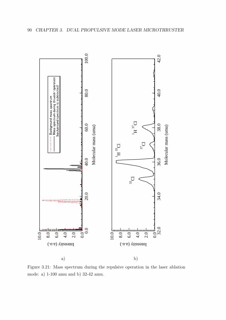
90 CHAPTER 3. DUAL PROPULSIVE MODE LASER MICROTHRUSTER
10.0 8.0
6.0
4.0
2.0
0.0
Intensity (a.u.)
100.
080
.060
.040
.020
.00.
0
Mol
ecul
ar m
ass
(um
a)
Backgro
und m
ass s
pactr
um
Mass s
pectr
um
during t
hru
ste
r opera
tion
(backgro
und s
pectr
um
is s
ubtr
acte
d)
a)
10.0 8.0
6.0
4.0
2.0
0.0
Intensity (a.u.)
42.0
40.0
38.0
36.0
34.0
32.0
Mol
ecul
ar m
ass
(um
a)
35C
l
37C
l
1 H 35
Cl
1 H 37
Cl
b)
Figure 3.21: Mass spectrum during the repulsive operation in the laser ablation
mode: a) 1-100 amu and b) 32-42 amu.
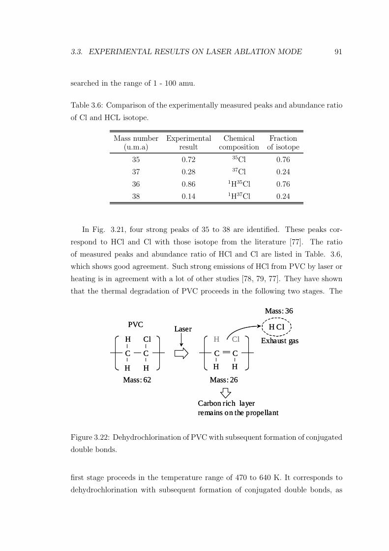
3.3. EXPERIMENTAL RESULTS ON LASER ABLATION MODE 91
searched in the range of 1 - 100 amu.
Table 3.6: Comparison of the experimentally measured peaks and abundance ratio
of Cl and HCL isotope.
Mass number Experimental Chemical Fraction(u.m.a) result composition of isotope
35 0.72 35Cl 0.76
37 0.28 37Cl 0.24
36 0.86 1H35Cl 0.76
38 0.14 1H37Cl 0.24
In Fig. 3.21, four strong peaks of 35 to 38 are identified. These peaks cor-
respond to HCl and Cl with those isotope from the literature [77]. The ratio
of measured peaks and abundance ratio of HCl and Cl are listed in Table. 3.6,
which shows good agreement. Such strong emissions of HCl from PVC by laser or
heating is in agreement with a lot of other studies [78, 79, 77]. They have shown
that the thermal degradation of PVC proceeds in the following two stages. The
Mass: 62
PVC
C C
HH
H Cl
C C
HH
H Cl
H ClLaser
Exhaust gas
Mass: 26
Mass: 36
Carbon rich layerremains on the propellant
Mass: 62
PVC
C C
HH
H Cl
C C
HH
H Cl
H ClLaser
Exhaust gas
Mass: 26
Mass: 36
Carbon rich layerremains on the propellant
Figure 3.22: Dehydrochlorination of PVC with subsequent formation of conjugated
double bonds.
first stage proceeds in the temperature range of 470 to 640 K. It corresponds to
dehydrochlorination with subsequent formation of conjugated double bonds, as
92 CHAPTER 3. DUAL PROPULSIVE MODE LASER MICROTHRUSTER
shown in Fig 3.22. The second stage proceeds in 640 - 770 K, which is scission of
polyene sequences formed during the first stage. Therefore the ablated gas by a
diode laser would mainly consist of HCl, at least in the early stage of the ablation.
This preferential degradation of HCl in low temperature would explains the
reason for the decrease of impulse by multiple shot at the sample point. During
the laser ablation, HCl is degraded and other components are remained in PVC
as residuals. Once the heating is stopped, the residuals are cooled. When the
same point is again irradiated by laser, the residuals have to be heated again and,
after the re-heating, HCl would begin to degrade. On the other hand, if the same
point is continuously heated, laser can continuously heat the solid since residuals
are kept hot. Hence the duration time between shots would be important factor
determining the impulse bit of second shot.
3.4. DISCUSSION ON MECHANISM OF DIODE LASER ABLATION. 93
3.4 Discussion on Mechanism of Diode Laser Ab-
lation.
3.4.1 Analytical solutions of heat conduction by laser ir-
radiation
To clarify the ablation mechanism by diode laser irradiation, photothermal abla-
tion model is applied on the laser ablation processes. Here, it is assumed that
laser beam irradiated on the ablative propellant is converted from photo energy to
thermal energy by the absorption. It is because the laser intensity of diode laser is
not enough high to occur photochemical reaction. Hence the beam behaves as heat
source in the ablative material, and it is analyzed as heat conduction problem.
The laser ablation processes is assumed to be constructed by the following
regimes. First laser beam is absorbed in the ablative material and all the energy
is used to raise the inner temperature: heating regime. When the maximum
temperature, generally surface temperature, reaches to the boiling or degrading
temperature, the laser energy is used for both temperature raising and material
vaporization. This is transition regime. After enough time is pasted, the ablation
reaches to the stationary ablation, where the temperature profile recedes inward
with maintaining its shape, which is stationary ablation regime.
In this section, the above regimes are analyzed by the method of heat conduc-
tion problem where laser is treated as a heat source.
Heating regime
Heating of ablative material by laser irradiation can be described as one dimen-
sional semi-infinite heat conduction. The absorption of radiation in the first ap-
proximation obeys the Bouguer-Lambert-Beer law, that is the beam exponentially
decays. Hence the governing equation is
∂T
∂t= κ
∂2T
∂x2 +q
ρcpλae−x/λa (3.4)
i.c. T (x, 0) = 0, x ≥ 0 (3.5)
b.c.∂T
∂x
∣∣∣∣∣x=0
= 0,∂T
∂x
∣∣∣∣∣x=∞
= 0 (3.6)
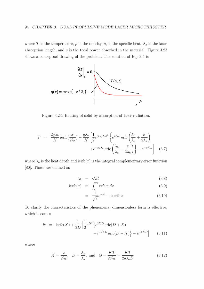
94 CHAPTER 3. DUAL PROPULSIVE MODE LASER MICROTHRUSTER
where T is the temperature, ρ is the density, cp is the specific heat, λa is the laser
absorption length, and q is the total power absorbed in the material. Figure 3.23
shows a conceptual drawing of the problem. The solution of Eq. 3.4 is
),( txT
x
00
=∂∂
x
T
( )axqxq λ/exp)( −=
),( txT
x
00
=∂∂
x
T
( )axqxq λ/exp)( −=
Figure 3.23: Heating of solid by absorption of laser radiation.
T =2qλh
Kierfc(
x
2λh) +
qλa
K
[1
2e(λh/λa)2
ex/λa erfc
(λh
λa+
x
2λh
)
+e−x/λa erfc
(λh
λa− x
2λh
)− e−x/λa
](3.7)
where λh is the heat depth and ierfc(x) is the integral complementary error function
[80]. Those are defined as
λh =√
κt (3.8)
ierfc(x) ≡∫ ∞
xerfcx dx (3.9)
=1√π
e−x2 − x erfcx (3.10)
To clarify the characteristics of the phenomena, dimensionless form is effective,
which becomes
Θ = ierfc(X) +1
2D
[1
2eD2
e2XD erfc(D + X)
+e−2XD erfc(D − X)− e−2XD
](3.11)
where
X =x
2λh, D =
λh
λa, and Θ =
KT
2qλh=
KT
2qλaD(3.12)
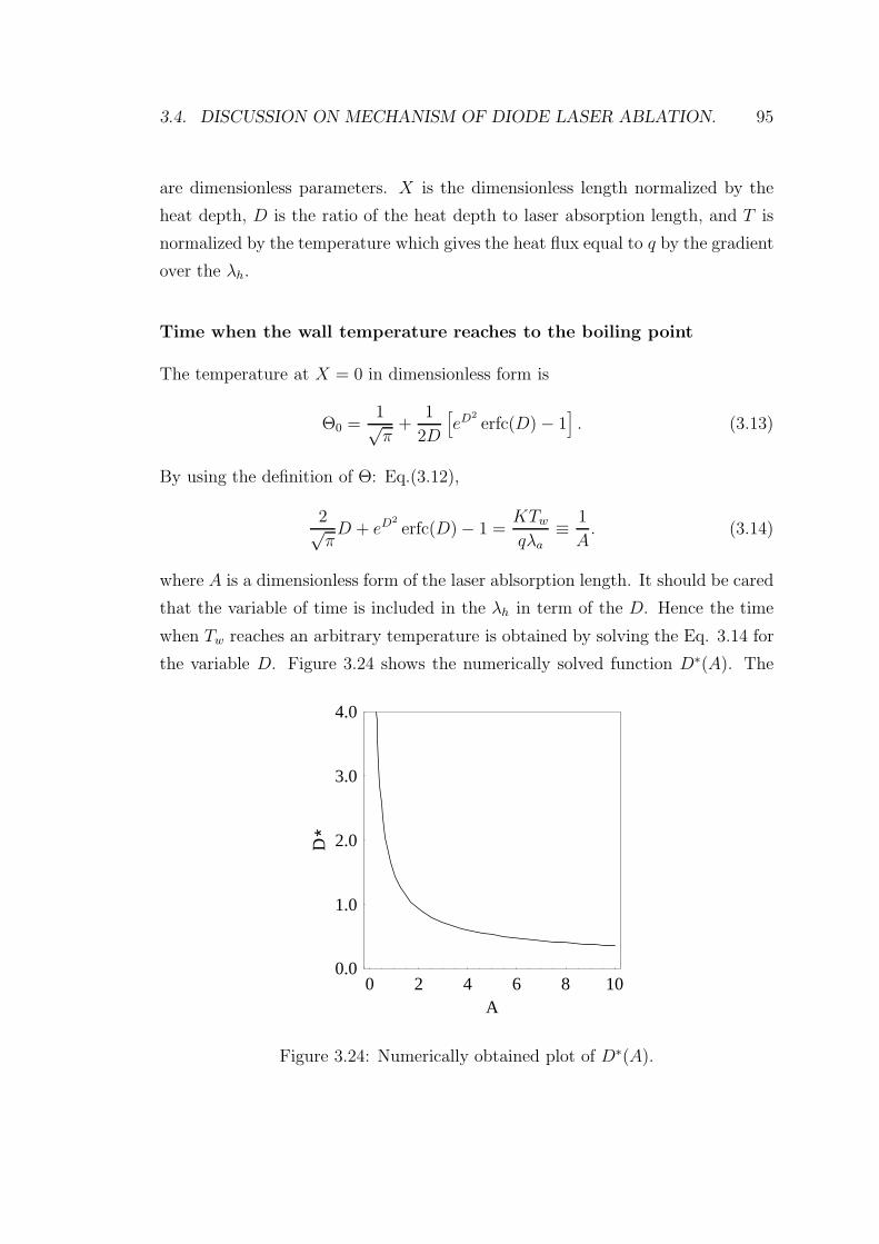
3.4. DISCUSSION ON MECHANISM OF DIODE LASER ABLATION. 95
are dimensionless parameters. X is the dimensionless length normalized by the
heat depth, D is the ratio of the heat depth to laser absorption length, and T is
normalized by the temperature which gives the heat flux equal to q by the gradient
over the λh.
Time when the wall temperature reaches to the boiling point
The temperature at X = 0 in dimensionless form is
Θ0 =1√π
+1
2D
[eD2
erfc(D) − 1]. (3.13)
By using the definition of Θ: Eq.(3.12),
2√π
D + eD2
erfc(D) − 1 =KTw
qλa≡ 1
A. (3.14)
where A is a dimensionless form of the laser ablsorption length. It should be cared
that the variable of time is included in the λh in term of the D. Hence the time
when Tw reaches an arbitrary temperature is obtained by solving the Eq. 3.14 for
the variable D. Figure 3.24 shows the numerically solved function D∗(A). The
0 2 4 6 8 10A
0.0
1.0
2.0
3.0
4.0
D*
Figure 3.24: Numerically obtained plot of D∗(A).
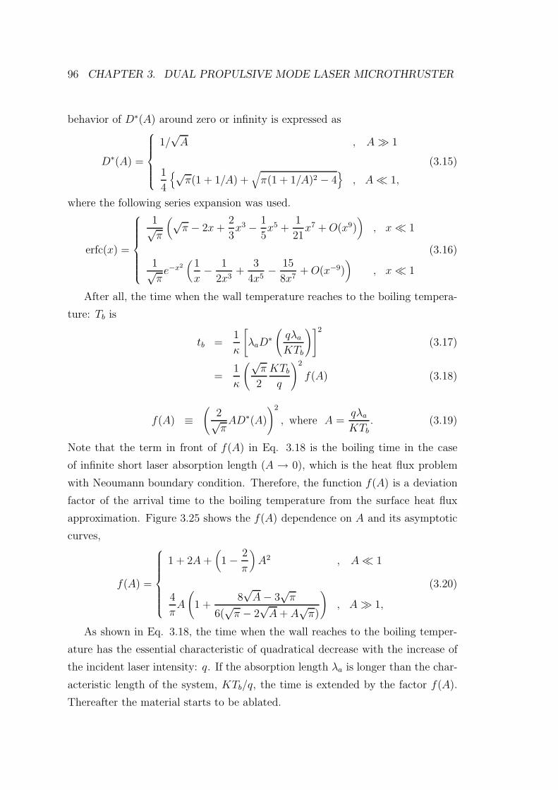
96 CHAPTER 3. DUAL PROPULSIVE MODE LASER MICROTHRUSTER
behavior of D∗(A) around zero or infinity is expressed as
D∗(A) =
⎧⎪⎪⎪⎪⎨⎪⎪⎪⎪⎩
1/√
A , A 1
1
4
√π(1 + 1/A) +
√π(1 + 1/A)2 − 4
, A 1,
(3.15)
where the following series expansion was used.
erfc(x) =
⎧⎪⎪⎪⎪⎪⎪⎨⎪⎪⎪⎪⎪⎪⎩
1√π
(√π − 2x +
2
3x3 − 1
5x5 +
1
21x7 + O(x9)
), x 1
1√π
e−x2(
1
x− 1
2x3+
3
4x5− 15
8x7+ O(x−9)
), x 1
(3.16)
After all, the time when the wall temperature reaches to the boiling tempera-
ture: Tb is
tb =1
κ
[λaD
∗(
qλa
KTb
)]2
(3.17)
=1
κ
(√π
2
KTb
q
)2
f(A) (3.18)
f(A) ≡(
2√π
AD∗(A)
)2
, where A =qλa
KTb. (3.19)
Note that the term in front of f(A) in Eq. 3.18 is the boiling time in the case
of infinite short laser absorption length (A → 0), which is the heat flux problem
with Neoumann boundary condition. Therefore, the function f(A) is a deviation
factor of the arrival time to the boiling temperature from the surface heat flux
approximation. Figure 3.25 shows the f(A) dependence on A and its asymptotic
curves,
f(A) =
⎧⎪⎪⎪⎪⎪⎪⎨⎪⎪⎪⎪⎪⎪⎩
1 + 2A +(1 − 2
π
)A2 , A 1
4
πA
(1 +
8√
A − 3√
π
6(√
π − 2√
A + A√
π)
), A 1,
(3.20)
As shown in Eq. 3.18, the time when the wall reaches to the boiling temper-
ature has the essential characteristic of quadratical decrease with the increase of
the incident laser intensity: q. If the absorption length λa is longer than the char-
acteristic length of the system, KTb/q, the time is extended by the factor f(A).
Thereafter the material starts to be ablated.
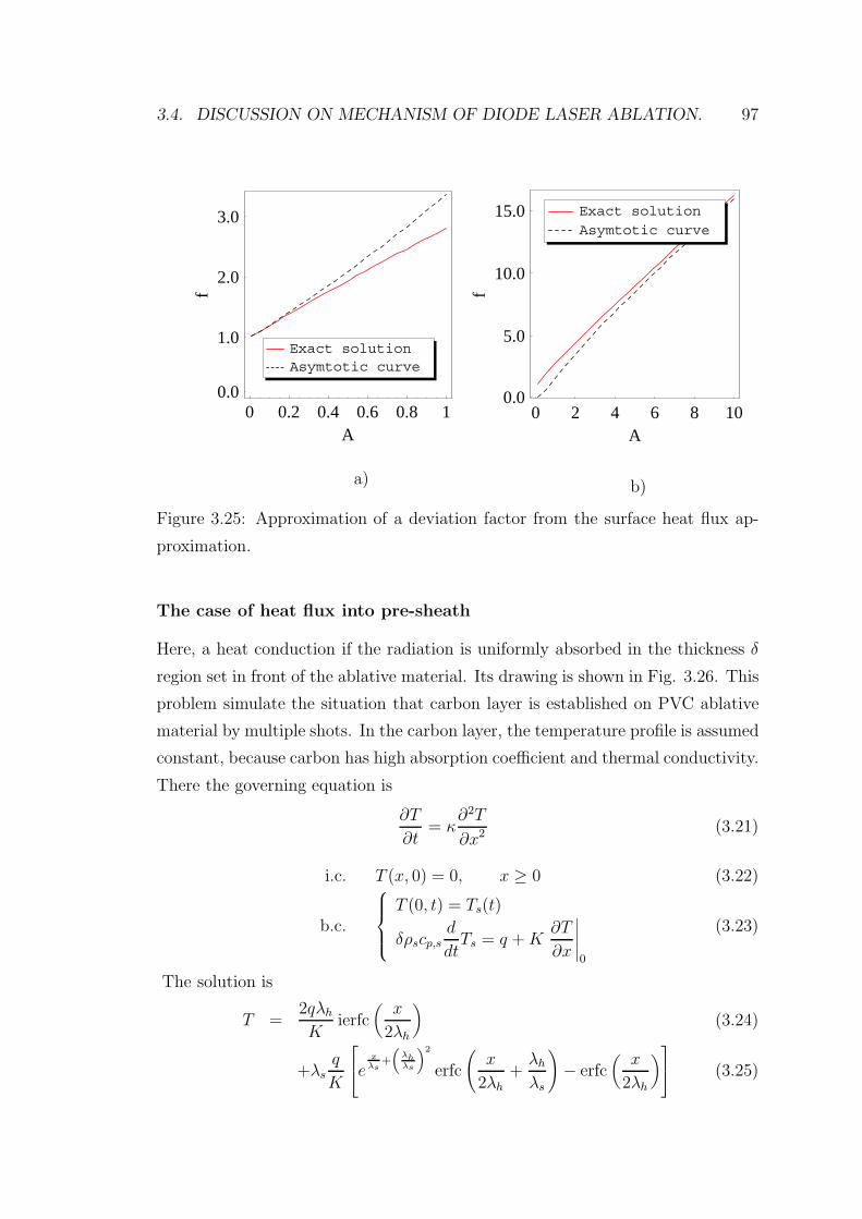
3.4. DISCUSSION ON MECHANISM OF DIODE LASER ABLATION. 97
0 0.2 0.4 0.6 0.8 1A
0.0
1.0
2.0
3.0f
Asymtotic curveExact solution
a)
0 2 4 6 8 10A
0.0
5.0
10.0
15.0
f
Asymtotic curve
Exact solution
b)
Figure 3.25: Approximation of a deviation factor from the surface heat flux ap-
proximation.
The case of heat flux into pre-sheath
Here, a heat conduction if the radiation is uniformly absorbed in the thickness δ
region set in front of the ablative material. Its drawing is shown in Fig. 3.26. This
problem simulate the situation that carbon layer is established on PVC ablative
material by multiple shots. In the carbon layer, the temperature profile is assumed
constant, because carbon has high absorption coefficient and thermal conductivity.
There the governing equation is
∂T
∂t= κ
∂2T
∂x2 (3.21)
i.c. T (x, 0) = 0, x ≥ 0 (3.22)
b.c.
⎧⎪⎪⎨⎪⎪⎩
T (0, t) = Ts(t)
δρscp,sd
dtTs = q + K
∂T
∂x
∣∣∣∣∣0
(3.23)
The solution is
T =2qλh
Kierfc
(x
2λh
)(3.24)
+λsq
K
⎡⎣e x
λs+
(λhλs
)2
erfc
(x
2λh
+λh
λs
)− erfc
(x
2λh
)⎤⎦ (3.25)
98 CHAPTER 3. DUAL PROPULSIVE MODE LASER MICROTHRUSTER
sρ
q
spc ,
δ
sT
),( txT
x
0x
TK
∂∂−
sρ
q
spc ,
δ
sT
),( txT
x
0x
TK
∂∂−
Figure 3.26: Pre-sheath heat conduction.
Θ = ierfc(X) +1
2Ds
[e2XDs+D2
s erfc(X + Ds) − erfc(X)]
(3.26)
where
λs =ρscp,s
ρcpδ, Θ =
KT
2qλs, X =
x
2λh, Ds =
λh
λs. (3.27)
Θ =2√π
+1
2Ds
[eD2
s erfc(Ds) − 1]
at x = 0 (3.28)
This equation is the same as Eq. 3.14 except for Ds instead of D. Therefore the
behavior of the temperature profile is the same as the case of Bouguer-Lambert-
Beer law absorption.
Stationary ablation
Next, recession velocity of the ablated surface is obtained in the stationary ablation
regime. The recession velocity during stationary ablation is independent on the
absorption length of laser, more generally, independent on the profile of heat
injection. Consider an arbitrary temperature distribution: T (x), which recedes
in the x direction with keeping the shape at the velocity of v, because now the
stationary ablation is assumed. After the surface recession of ∆x, the temperature
distribution becomes T (x − ∆x) as shown in Fig. 3.27. At the point of x, to
perform this recession, the temperature must be raised up to T (x − ∆x) from
T (x). Therefore, over the all x, the heat of
ρcp
∫ ∞
xw
T (x− ∆x) − T (x) dx (3.29)
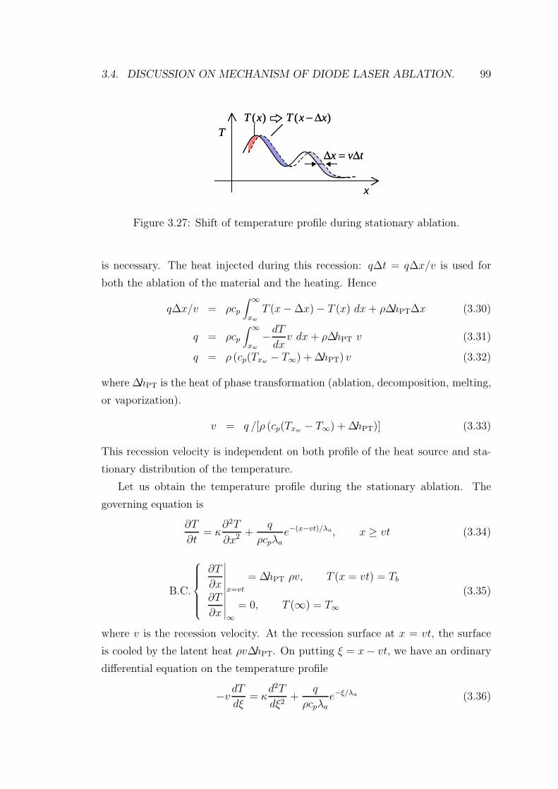
3.4. DISCUSSION ON MECHANISM OF DIODE LASER ABLATION. 99
)(xT )( xxT ∆−
tvx ∆=∆
T
x
)(xT )( xxT ∆−
tvx ∆=∆
T
x
Figure 3.27: Shift of temperature profile during stationary ablation.
is necessary. The heat injected during this recession: q∆t = q∆x/v is used for
both the ablation of the material and the heating. Hence
q∆x/v = ρcp
∫ ∞
xw
T (x− ∆x) − T (x) dx + ρ∆hPT∆x (3.30)
q = ρcp
∫ ∞
xw
−dT
dxv dx + ρ∆hPT v (3.31)
q = ρ (cp(Txw − T∞) + ∆hPT) v (3.32)
where ∆hPT is the heat of phase transformation (ablation, decomposition, melting,
or vaporization).
v = q /[ρ (cp(Txw − T∞) + ∆hPT)] (3.33)
This recession velocity is independent on both profile of the heat source and sta-
tionary distribution of the temperature.
Let us obtain the temperature profile during the stationary ablation. The
governing equation is
∂T
∂t= κ
∂2T
∂x2 +q
ρcpλae−(x−vt)/λa, x ≥ vt (3.34)
B.C.
⎧⎪⎪⎪⎪⎨⎪⎪⎪⎪⎩
∂T
∂x
∣∣∣∣∣x=vt
= ∆hPT ρv, T (x = vt) = Tb
∂T
∂x
∣∣∣∣∣∞ = 0, T (∞) = T∞(3.35)
where v is the recession velocity. At the recession surface at x = vt, the surface
is cooled by the latent heat ρv∆hPT. On putting ξ = x− vt, we have an ordinary
differential equation on the temperature profile
−vdT
dξ= κ
d2T
dξ2+
q
ρcpλae−ξ/λa (3.36)
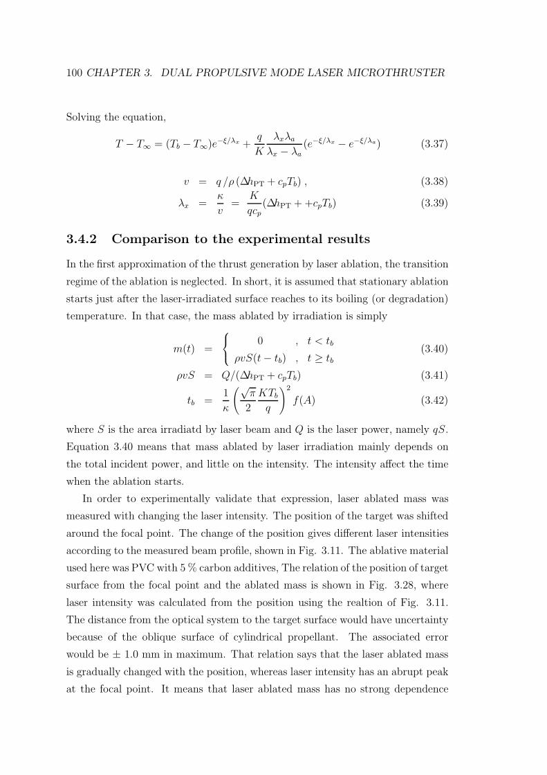
100 CHAPTER 3. DUAL PROPULSIVE MODE LASER MICROTHRUSTER
Solving the equation,
T − T∞ = (Tb − T∞)e−ξ/λx +q
K
λxλa
λx − λa(e−ξ/λx − e−ξ/λa) (3.37)
v = q /ρ (∆hPT + cpTb) , (3.38)
λx =κ
v=
K
qcp(∆hPT + +cpTb) (3.39)
3.4.2 Comparison to the experimental results
In the first approximation of the thrust generation by laser ablation, the transition
regime of the ablation is neglected. In short, it is assumed that stationary ablation
starts just after the laser-irradiated surface reaches to its boiling (or degradation)
temperature. In that case, the mass ablated by irradiation is simply
m(t) =
⎧⎨⎩ 0 , t < tb
ρvS(t − tb) , t ≥ tb
(3.40)
ρvS = Q/(∆hPT + cpTb) (3.41)
tb =1
κ
(√π
2
KTb
q
)2
f(A) (3.42)
where S is the area irradiatd by laser beam and Q is the laser power, namely qS.
Equation 3.40 means that mass ablated by laser irradiation mainly depends on
the total incident power, and little on the intensity. The intensity affect the time
when the ablation starts.
In order to experimentally validate that expression, laser ablated mass was
measured with changing the laser intensity. The position of the target was shifted
around the focal point. The change of the position gives different laser intensities
according to the measured beam profile, shown in Fig. 3.11. The ablative material
used here was PVC with 5 % carbon additives, The relation of the position of target
surface from the focal point and the ablated mass is shown in Fig. 3.28, where
laser intensity was calculated from the position using the realtion of Fig. 3.11.
The distance from the optical system to the target surface would have uncertainty
because of the oblique surface of cylindrical propellant. The associated error
would be ± 1.0 mm in maximum. That relation says that the laser ablated mass
is gradually changed with the position, whereas laser intensity has an abrupt peak
at the focal point. It means that laser ablated mass has no strong dependence
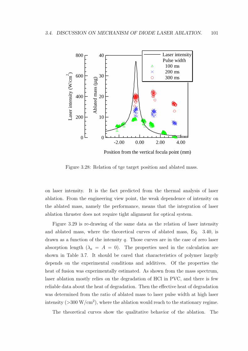
3.4. DISCUSSION ON MECHANISM OF DIODE LASER ABLATION. 101
40
30
20
10
0
Abl
ated
mas
s (µ
g)
4.002.000.00-2.00
Position from the vertical focula point (mm)
800
600
400
200
0
Las
er in
tens
ity (
W/c
m2 )
Laser intensity Pulse width
100 ms 200 ms 300 ms
Figure 3.28: Relation of tge target position and ablated mass.
on laser intensity. It is the fact predicted from the thermal analysis of laser
ablation. From the engineering view point, the weak dependence of intensity on
the ablated mass, namely the performance, means that the integration of laser
ablation thruster does not require tight alignment for optical system.
Figure 3.29 is re-drawing of the same data as the relation of laser intensity
and ablated mass, where the theoretical curves of ablated mass, Eq. 3.40, is
drawn as a function of the intensity q. Those curves are in the case of zero laser
absorption length (λa = A = 0). The properties used in the calculation are
shown in Table 3.7. It should be cared that characteristics of polymer largely
depends on the experimental conditions and additives. Of the properties the
heat of fusion was experimentally estimated. As shown from the mass spectrum,
laser ablation mostly relies on the degradation of HCl in PVC, and there is few
reliable data about the heat of degradation. Then the effective heat of degradation
was determined from the ratio of ablated mass to laser pulse width at high laser
intensity (>300 W/cm2), where the ablation would reach to the stationary regime.
The theoretical curves show the qualitative behavior of the ablation. The
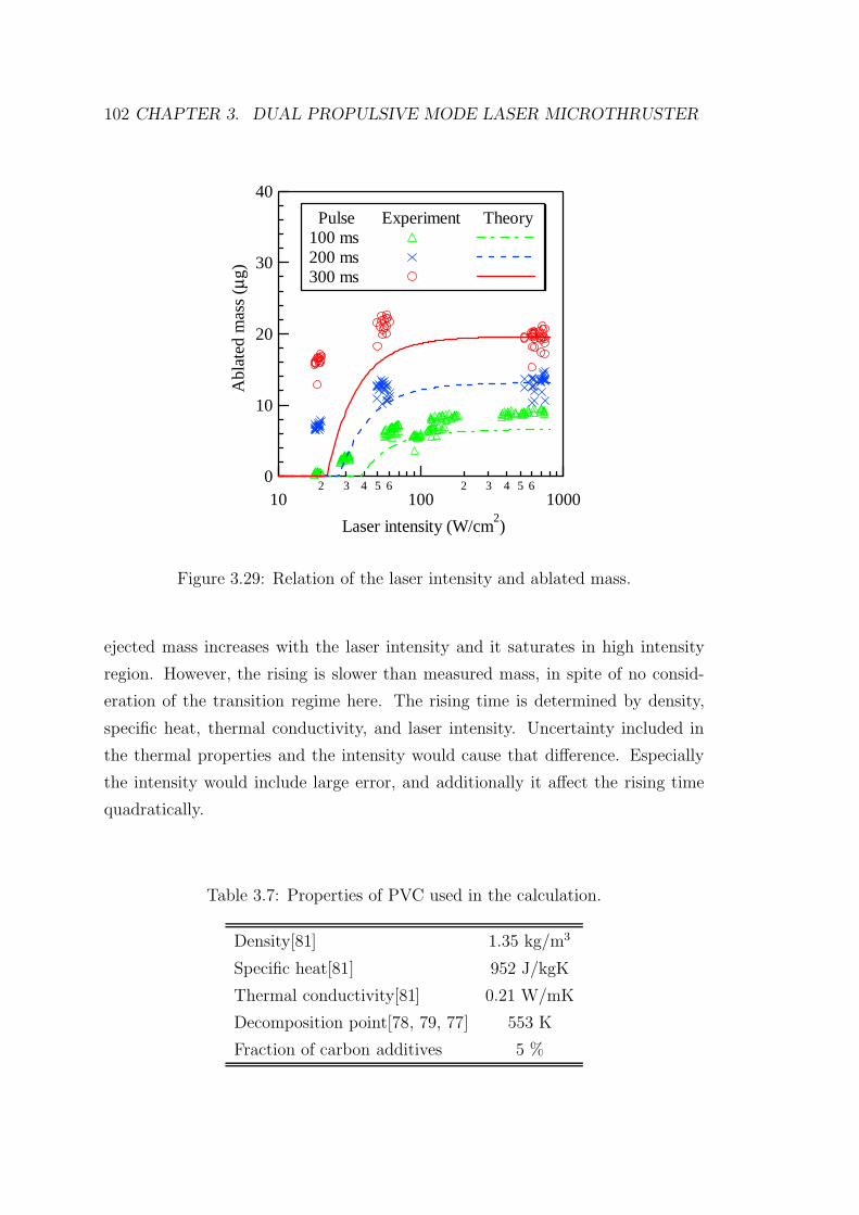
102 CHAPTER 3. DUAL PROPULSIVE MODE LASER MICROTHRUSTER
40
30
20
10
0
Abl
ated
mas
s (µ
g)
102 3 4 5 6
1002 3 4 5 6
1000
Laser intensity (W/cm2)
Pulse Experiment Theory 100 ms 200 ms 300 ms
Figure 3.29: Relation of the laser intensity and ablated mass.
ejected mass increases with the laser intensity and it saturates in high intensity
region. However, the rising is slower than measured mass, in spite of no consid-
eration of the transition regime here. The rising time is determined by density,
specific heat, thermal conductivity, and laser intensity. Uncertainty included in
the thermal properties and the intensity would cause that difference. Especially
the intensity would include large error, and additionally it affect the rising time
quadratically.
Table 3.7: Properties of PVC used in the calculation.
Density[81] 1.35 kg/m3
Specific heat[81] 952 J/kgK
Thermal conductivity[81] 0.21 W/mK
Decomposition point[78, 79, 77] 553 K
Fraction of carbon additives 5 %
3.5. EXPERIMENTAL RESULTS ON LASER IGNITION MODE 103
3.5 Experimental Results on Laser Ignition Mode
3.5.1 Laser ignition of pyrotechnics
Three varieties of pyrotechnics were prepared for the laser ignition mode experi-
ments: composite propellant, double-base propellant, and pelleted boron/potassium
nitrate(B/KNO3). These pyrotechnics were loaded into the holes on the ceramic
cylinder (shown in Fig. 3.13). The composite and double-base propellants were
cut to the appropriate size and pressed into the 2.0-mm-diam, 1.0-mm-long holes.
Pelleted B/KNO3 cylinders of 3.2-mm-diam and 2.0-mm-long were installed in
holes of the corresponding size. The pellet weighed 0.03 g. Pictures of the three
pyrotechnics are shown in Fig. 3.30.
Composite propellant
Double-base propellant
B/KNO3 pellets
D:10.2 mmL: 6.0 mm
D:3.2 mmL:2.0 mm
Composite propellant
Double-base propellant
B/KNO3 pellets
D:10.2 mmL: 6.0 mm
D:3.2 mmL:2.0 mm
Figure 3.30: Pictures of the pyrotechnics: composite propellant, double-base pro-
pellant, and pelleted boron/potassium niterate (B/KNO3).
In the atmosphere, all pyrotechnics were successfully ignited by the irradiation
from a diode laser. Figure 3.31 a) shows images of laser ignited combustion of
the composite propellant in the atmosphere. The origin of the time in the figure
is when the laser irradiation starts. Initially, laser beam irradiates the propellant
and there is no reaction (t = 0 ∼ 400ms). After 500 ms, the propellant undergoes
combustion with exhausting intense plume and it lasts to t = 1000 ms.
However, in vacuum, composite and double-base propellants were not ignited.
Figure 3.31 b) shows images when the composite propellant was irradiated by laser
in vacuum. Self-sustained combustion was not performed, whereas several small
sparks were scattered from the laser irradiation point. The scattering of sparks
goes only under laser irradiation. Generally, the combustion speed of pyrotechnics
decreases with decrease of the background pressure, and several pyrotechnics have
104 CHAPTER 3. DUAL PROPULSIVE MODE LASER MICROTHRUSTER
a threshold pressure for the self-combustion.
t = 100 ms
t = 1100 ms
t = 200 ms
t = 300 ms
t = 400 ms
t = 500 ms
t = 600 ms
t = 700 ms
t = 800 ms
t = 900 ms
t = 1000 ms
t = 100 ms
t = 200 ms
t = 300 ms
t = 400 ms
t = 500 ms
t = 600 ms
t = 700 ms
t = 800 ms
t = 900 ms
Laser emission
LD focusing tube
Laser beam
t = 100 ms
t = 1100 ms
t = 200 ms
t = 300 ms
t = 400 ms
t = 500 ms
t = 600 ms
t = 700 ms
t = 800 ms
t = 900 ms
t = 1000 ms
t = 100 ms
t = 1100 ms
t = 200 ms
t = 300 ms
t = 400 ms
t = 500 ms
t = 600 ms
t = 700 ms
t = 800 ms
t = 900 ms
t = 1000 ms
t = 100 ms
t = 1100 ms
t = 200 ms
t = 300 ms
t = 400 ms
t = 500 ms
t = 600 ms
t = 700 ms
t = 800 ms
t = 900 ms
t = 1000 ms
t = 100 ms
t = 200 ms
t = 300 ms
t = 400 ms
t = 500 ms
t = 600 ms
t = 700 ms
t = 800 ms
t = 900 ms
t = 100 ms
t = 200 ms
t = 300 ms
t = 400 ms
t = 500 ms
t = 600 ms
t = 700 ms
t = 800 ms
t = 900 ms
Laser emission
LD focusing tube
Laser beam
a) b)
Figure 3.31: Laser irradiation of composite propellant; a) Laser ignited combustion
in the atmosphere and b) no self-sustained combustion in vacuum.
In contrast, B/KNO3 was successfully ignited by diode laser beam under a
background pressure of 1.4 - 3.0 × 10⁻⁴ Torr. Figure 3.32 shows images of the
laser ignition of a B/KNO3 pellet. Initially, the laser beam irradiates the pellet
(t = 30 ms in Fig. 3.32). The pellet then undergoes combustion at the focal point
of the laser beam (t = 90 ms). The combustion front spreads over the surface of
the pellet and steady combustion lasts during t = 270 ∼ 690ms. Thereafter the
combustion becomes weak and terminates at approximately 1000 ms. Table 3.8
3.5. EXPERIMENTAL RESULTS ON LASER IGNITION MODE 105
t = 30 ms
t = 510 ms
t = 450 ms
t = 390 ms
t = 330 ms
t = 270 ms
t = 210 ms
t = 150 ms
t = 90 ms
t = 570 ms
t = 1050 ms
t = 990 ms
t = 930ms
t = 870 ms
t = 810 ms
t = 750 ms
t = 690 ms
t = 630 ms
Reflection on the protective window
Laser emission
t = 30 ms
t = 510 ms
t = 450 ms
t = 390 ms
t = 330 ms
t = 270 ms
t = 210 ms
t = 150 ms
t = 90 ms
t = 30 ms
t = 510 ms
t = 450 ms
t = 390 ms
t = 330 ms
t = 270 ms
t = 210 ms
t = 150 ms
t = 90 ms
t = 570 ms
t = 1050 ms
t = 990 ms
t = 930ms
t = 870 ms
t = 810 ms
t = 750 ms
t = 690 ms
t = 630 ms
t = 570 ms
t = 1050 ms
t = 990 ms
t = 930ms
t = 870 ms
t = 810 ms
t = 750 ms
t = 690 ms
t = 630 ms
Reflection on the protective window
Laser emission
Figure 3.32: Laser ignited combustion of B/KNO3 in vacuum.
106 CHAPTER 3. DUAL PROPULSIVE MODE LASER MICROTHRUSTER
summarizes the results of laser irradiation of pyrotechnics.
Table 3.8: Summery of 300 mW laser irradiation on pyrotechnics.
Pyrotechnics in the atmosphere in vacuum (< 10−3 Torr)
Composite propellant Combustion No self-sustained combustion
Double-base propellant Combustion No self-sustained combustion
Boron/potassium nitrate Combustion Combustion
3.5.2 Laser ignition probability of B/KNO3 in vacuum
Effect of laser pulse width
The ignition threshold of B/KNO3 was investigated against the laser pulse width;
the results are shown in Figure 3.33. The laser power was 250 mW. There the
ignition probability is defined as the number of ignitions over number of trials.
At laser pulses shorter than 50 ms, no propellant was ignited. Between 50 to 150
ms, the propellants were ignited only after several attempts. When the laser pulse
width exceeded 150 ms (38 mJ), all the propellants were successfully ignited.
The ignition threshold of our solid propellant was therefore about 100ms. The
uncertainty of the ignition around the threshold was caused by slight differences
in the experimental conditions, surface position and angle of propellants, and so
on, and depends on the alignment accuracy of the optical system. A pulse width
of 1000 ms (250 mJ) would be enough for spacecraft applications.
Effect of laser power
The effect of laser power on the ignition probability was investigated. To remove
the variation of the position and angle of the pellets, another propellant feeding
system was prepared. It was designed not for the thruster but only for accurate
evaluation of the ignition probability dependence of the power. Figure 3.34 shows
the picture of the experiment setup. Twenty pellets are installed into holes aligned
on a line, and each pellets are separated by plastic walls. Laser beam enters
through a acrylic window which prevents the optical system from fouling. The
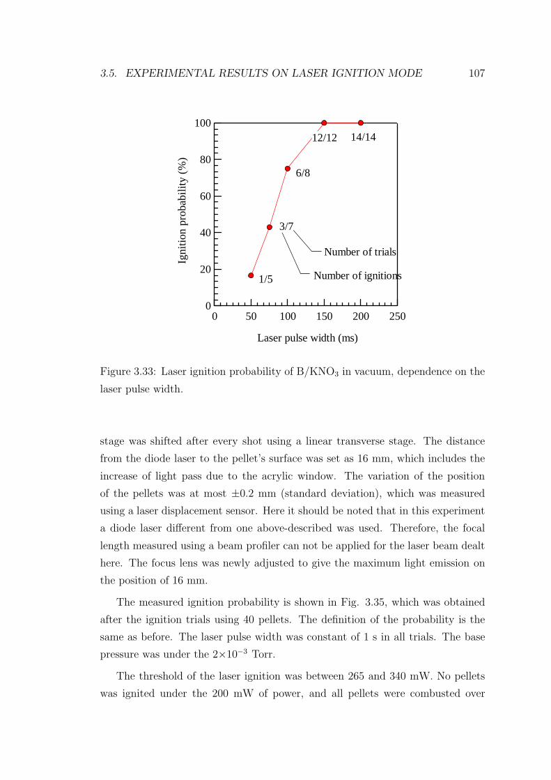
3.5. EXPERIMENTAL RESULTS ON LASER IGNITION MODE 107
100
80
60
40
20
0
Igni
tion
pro
babi
lity
(%
)
250200150100500
Laser pulse width (ms)
Number of ignitions
Number of trials
1/5
3/7
6/8
14/1412/12
Figure 3.33: Laser ignition probability of B/KNO3 in vacuum, dependence on the
laser pulse width.
stage was shifted after every shot using a linear transverse stage. The distance
from the diode laser to the pellet’s surface was set as 16 mm, which includes the
increase of light pass due to the acrylic window. The variation of the position
of the pellets was at most ±0.2 mm (standard deviation), which was measured
using a laser displacement sensor. Here it should be noted that in this experiment
a diode laser different from one above-described was used. Therefore, the focal
length measured using a beam profiler can not be applied for the laser beam dealt
here. The focus lens was newly adjusted to give the maximum light emission on
the position of 16 mm.
The measured ignition probability is shown in Fig. 3.35, which was obtained
after the ignition trials using 40 pellets. The definition of the probability is the
same as before. The laser pulse width was constant of 1 s in all trials. The base
pressure was under the 2×10⁻³ Torr.
The threshold of the laser ignition was between 265 and 340 mW. No pellets
was ignited under the 200 mW of power, and all pellets were combusted over
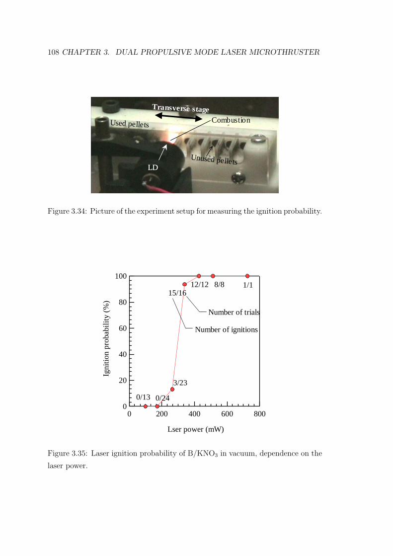
108 CHAPTER 3. DUAL PROPULSIVE MODE LASER MICROTHRUSTER
Unused pellets
Combustion
LDLD
Used pellets
Transverse stage
Unused pellets
Combustion
LDLD
Used pellets
Transverse stage
Unused pellets
Combustion
LDLD
Used pellets
Transverse stage
Figure 3.34: Picture of the experiment setup for measuring the ignition probability.
100
80
60
40
20
0
Igni
tion
pro
babi
lity
(%
)
8006004002000
Lser power (mW)
0/13 0/24
3/23
15/1612/12 8/8 1/1
Number of trials
Number of ignitions
Figure 3.35: Laser ignition probability of B/KNO3 in vacuum, dependence on the
laser power.

3.5. EXPERIMENTAL RESULTS ON LASER IGNITION MODE 109
the 400 mW. The observed combustion processes were the same as Fig. 3.32.
After the laser irradiation and the ablation of the surface, the pellets started the
combustion, which lasts about 1s.
The obtained threshold power for the laser ignition was a little inconsistent
in the experiment of previous section 3.5.2, where the laser power 250 mW and
width 1 s gave exact ignition. The discrepancy would be caused by the difference
of configurations of laser optical assembly and feeding system. At most 500 mW
power, however, is enough power to ignite B/KNO3 pyrotechnics in vacuum. These
results says that the laser ignition mode can easily coexist with the laser ablation
mode because the energy required for ignition was lower than or comparable to
that for laser ablation.
3.5.3 Thrust measurement of laser ignition mode
Thrust measurement for laser ignition mode was performed to evaluate the thrust
produced by the combustion of laser ignited B/KNO3 pellet. The thruster used
for the thrust measurement was shown in Figs. 3.13 and 3.12. The B/KNO3 pellet
used here weighed 32 mg and installed into a ceramic hole without any nozzle.
Table 3.9 indicates performance in the laser ignition mode using B/KNO3
propellant in vacuum. The averaged impulse was 11±2 mNs and the specific
impulse, which was calculated using the weight of the pellet, was 36±7 s. The
theoretical predicted maximum specific impulse of B/KNO3 in vacuum was higher
than 100 s. This discrepancy probably arose because the propellant and the nozzle
were not optimized in shape. The consumed energy here for the laser ignition was
38 mJ using 250 mW laser power and 150 ms laser power.
Table 3.9: Result of thrust measurement of laser ignition mode using 30 mg
B/KNO3 pellets.
Impulse 11±2 mNs
Specific impulse 36±7 s
Laser energy 38 mJ (250 mW, 150 ms)
The thrust measurement described here have shown that dual operational
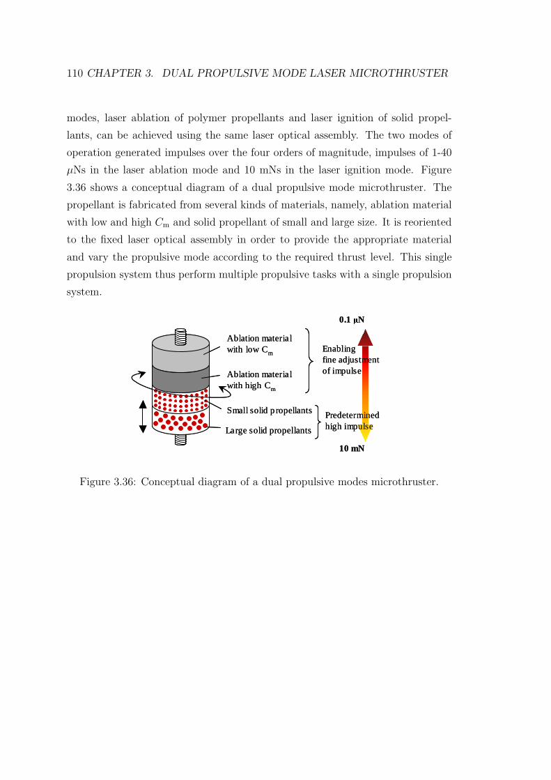
110 CHAPTER 3. DUAL PROPULSIVE MODE LASER MICROTHRUSTER
modes, laser ablation of polymer propellants and laser ignition of solid propel-
lants, can be achieved using the same laser optical assembly. The two modes of
operation generated impulses over the four orders of magnitude, impulses of 1-40
µNs in the laser ablation mode and 10 mNs in the laser ignition mode. Figure
3.36 shows a conceptual diagram of a dual propulsive mode microthruster. The
propellant is fabricated from several kinds of materials, namely, ablation material
with low and high Cm and solid propellant of small and large size. It is reoriented
to the fixed laser optical assembly in order to provide the appropriate material
and vary the propulsive mode according to the required thrust level. This single
propulsion system thus perform multiple propulsive tasks with a single propulsion
system.
Large solid propellants
Small solid p ropellants
Ablation material with high Cm
Ablation material with low Cm Enabling
fine adjustment of impulse
10 10 mNmN
0.1 0.1 µµNN
Predetermined high impulseLarge solid propellants
Small solid p ropellants
Ablation material with high Cm
Ablation material with low Cm Enabling
fine adjustment of impulse
10 10 mNmN
0.1 0.1 µµNN
Predetermined high impulse
Figure 3.36: Conceptual diagram of a dual propulsive modes microthruster.
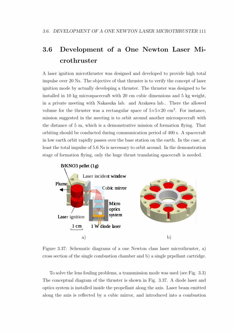
3.6. DEVELOPMENT OF A ONE NEWTON LASER MICROTHRUSTER 111
3.6 Development of a One Newton Laser Mi-
crothruster
A laser ignition microthruster was designed and developed to provide high total
impulse over 20 Ns. The objective of that thruster is to verify the concept of laser
ignition mode by actually developing a thruster. The thruster was designed to be
installed in 10 kg microspacecraft with 20 cm cubic dimensions and 5 kg weight,
in a private meeting with Nakasuka lab. and Arakawa lab.. There the allowed
volume for the thruster was a rectangular space of 5×5×20 cm3. For instance,
mission suggested in the meeting is to orbit around another microspcecraft with
the distance of 5 m, which is a demonstrative mission of formation flying. That
orbiting should be conducted during communication period of 400 s. A spacecraft
in low earth orbit rapidly passes over the base station on the earth. In the case, at
least the total impulse of 5.6 Ns is necessary to orbit around. In the demonstration
stage of formation flying, only the huge thrust translating spacecraft is needed.
B/KNO3 pellet (1g)
Laser ignition
1 W diode laser
Micro optics system
Plume
1 cm
Laser incident window
Cubic mirror
B/KNO3 pellet (1g)
Laser ignition
1 W diode laser
Micro optics system
Plume
1 cm
Laser incident window
Cubic mirror
B/KNO3 pellet (1g)
Laser ignition
1 W diode laser
Micro optics system
Plume
1 cm
Laser incident window
Cubic mirror
a) b)
Figure 3.37: Schematic diagrams of a one Newton class laser microthruster, a)
cross section of the single combustion chamber and b) a single prpellant cartridge.
To solve the lens fouling problems, a transmission mode was used (see Fig. 3.3)
The conceptual diagram of the thruster is shown in Fig. 3.37. A diode laser and
optics system is installed inside the propellant along the axis. Laser beam emitted
along the axis is reflected by a cubic mirror, and introduced into a combustion
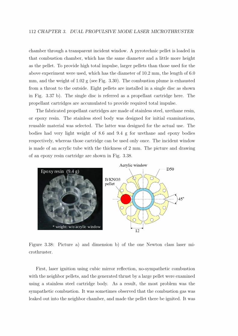
112 CHAPTER 3. DUAL PROPULSIVE MODE LASER MICROTHRUSTER
chamber through a transparent incident window. A pyrotechnic pellet is loaded in
that combustion chamber, which has the same diameter and a little more height
as the pellet. To provide high total impulse, larger pellets than those used for the
above experiment were used, which has the diameter of 10.2 mm, the length of 6.0
mm, and the weight of 1.02 g (see Fig. 3.30). The combustion plume is exhausted
from a throat to the outside. Eight pellets are installed in a single disc as shown
in Fig. 3.37 b). The single disc is referred as a propellant cartridge here. The
propellant cartridges are accumulated to provide required total impulse.
The fabricated propellant cartridges are made of stainless steel, urethane resin,
or epoxy resin. The stainless steel body was designed for initial examinations,
reusable material was selected. The latter was designed for the actual use. The
bodies had very light weight of 8.6 and 9.4 g for urethane and epoxy bodies
respectively, whereas those cartridge can be used only once. The incident window
is made of an acrylic tube with the thickness of 2 mm. The picture and drawing
of an epoxy resin cartridge are shown in Fig. 3.38.
Epoxy resin (9.4 g)
* weight: w/o acrylic window
Epoxy resin (9.4 g)
* weight: w/o acrylic window
Figure 3.38: Picture a) and dimension b) of the one Newton class laser mi-
crothruster.
First, laser ignition using cubic mirror reflection, no-sympathetic combustion
with the neighbor pellets, and the generated thrust by a large pellet were examined
using a stainless steel cartridge body. As a result, the most problem was the
sympathetic combustion. It was sometimes observed that the combustion gas was
leaked out into the neighbor chamber, and made the pellet there be ignited. It was
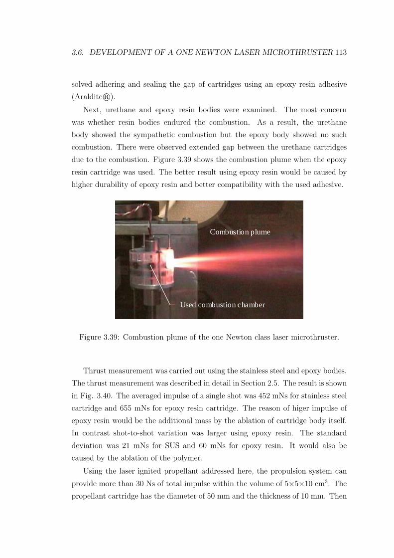
3.6. DEVELOPMENT OF A ONE NEWTON LASER MICROTHRUSTER 113
solved adhering and sealing the gap of cartridges using an epoxy resin adhesive
(Araldite r©).
Next, urethane and epoxy resin bodies were examined. The most concern
was whether resin bodies endured the combustion. As a result, the urethane
body showed the sympathetic combustion but the epoxy body showed no such
combustion. There were observed extended gap between the urethane cartridges
due to the combustion. Figure 3.39 shows the combustion plume when the epoxy
resin cartridge was used. The better result using epoxy resin would be caused by
higher durability of epoxy resin and better compatibility with the used adhesive.
Used combustion chamber
Combustion plume
Used combustion chamber
Combustion plume
Figure 3.39: Combustion plume of the one Newton class laser microthruster.
Thrust measurement was carried out using the stainless steel and epoxy bodies.
The thrust measurement was described in detail in Section 2.5. The result is shown
in Fig. 3.40. The averaged impulse of a single shot was 452 mNs for stainless steel
cartridge and 655 mNs for epoxy resin cartridge. The reason of higer impulse of
epoxy resin would be the additional mass by the ablation of cartridge body itself.
In contrast shot-to-shot variation was larger using epoxy resin. The standard
deviation was 21 mNs for SUS and 60 mNs for epoxy resin. It would also be
caused by the ablation of the polymer.
Using the laser ignited propellant addressed here, the propulsion system can
provide more than 30 Ns of total impulse within the volume of 5×5×10 cm3. The
propellant cartridge has the diameter of 50 mm and the thickness of 10 mm. Then
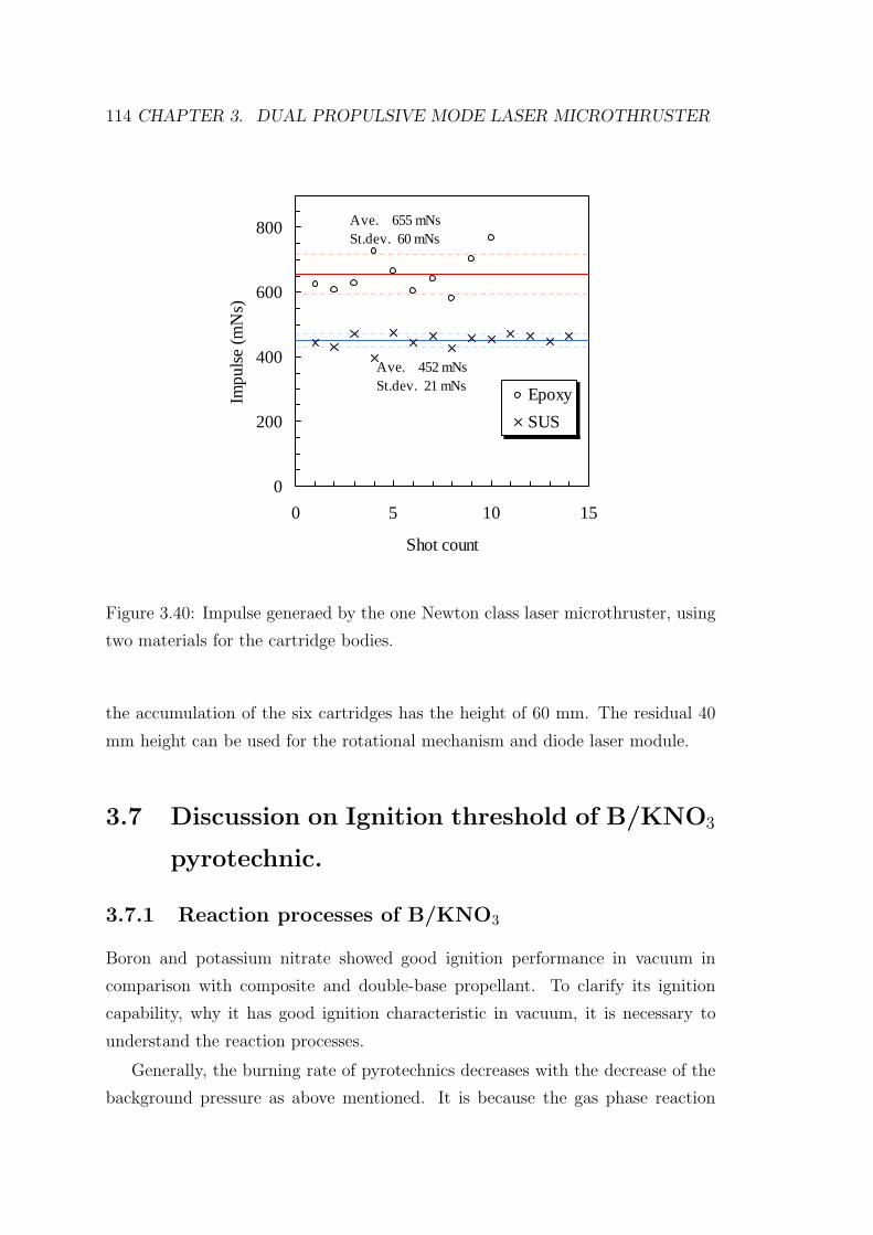
114 CHAPTER 3. DUAL PROPULSIVE MODE LASER MICROTHRUSTER
0
200
400
600
800
0 5 10 15
Shot count
Impu
lse
(mN
s)
.
Epoxy
SUS
Ave. 655 mNsSt.dev. 60 mNs
Ave. 452 mNsSt.dev. 21 mNs
Figure 3.40: Impulse generaed by the one Newton class laser microthruster, using
two materials for the cartridge bodies.
the accumulation of the six cartridges has the height of 60 mm. The residual 40
mm height can be used for the rotational mechanism and diode laser module.
3.7 Discussion on Ignition threshold of B/KNO3
pyrotechnic.
3.7.1 Reaction processes of B/KNO3
Boron and potassium nitrate showed good ignition performance in vacuum in
comparison with composite and double-base propellant. To clarify its ignition
capability, why it has good ignition characteristic in vacuum, it is necessary to
understand the reaction processes.
Generally, the burning rate of pyrotechnics decreases with the decrease of the
background pressure as above mentioned. It is because the gas phase reaction
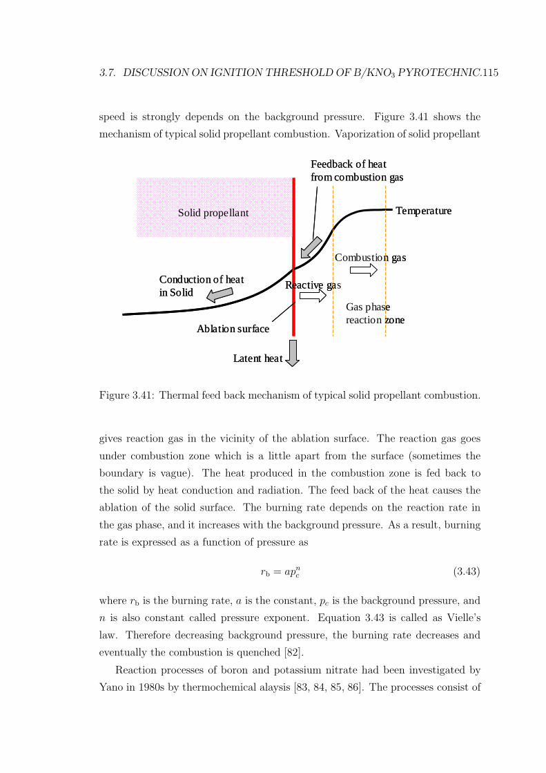
3.7. DISCUSSION ON IGNITION THRESHOLD OF B/KNO3 PYROTECHNIC.115
speed is strongly depends on the background pressure. Figure 3.41 shows the
mechanism of typical solid propellant combustion. Vaporization of solid propellant
Solid propellant Temperature
Gas phase reaction zone
Ablation surface
Reactive gas
Combustion gas
Conduction of heatin Solid
Feedback of heatfrom combustion gas
Latent heat
Solid propellant Temperature
Gas phase reaction zone
Ablation surface
Reactive gas
Combustion gas
Conduction of heatin Solid
Feedback of heatfrom combustion gas
Latent heat
Figure 3.41: Thermal feed back mechanism of typical solid propellant combustion.
gives reaction gas in the vicinity of the ablation surface. The reaction gas goes
under combustion zone which is a little apart from the surface (sometimes the
boundary is vague). The heat produced in the combustion zone is fed back to
the solid by heat conduction and radiation. The feed back of the heat causes the
ablation of the solid surface. The burning rate depends on the reaction rate in
the gas phase, and it increases with the background pressure. As a result, burning
rate is expressed as a function of pressure as
rb = apnc (3.43)
where rb is the burning rate, a is the constant, pc is the background pressure, and
n is also constant called pressure exponent. Equation 3.43 is called as Vielle’s
law. Therefore decreasing background pressure, the burning rate decreases and
eventually the combustion is quenched [82].
Reaction processes of boron and potassium nitrate had been investigated by
Yano in 1980s by thermochemical alaysis [83, 84, 85, 86]. The processes consist of
116 CHAPTER 3. DUAL PROPULSIVE MODE LASER MICROTHRUSTER
a three-stage reaction. A significant heat is produced in the first-stage process by
the reaction
B + KNO3 → KBO2 + NO. (3.44)
In the second-stage process, the remaining un-reacted potassium nitrate decom-
poses to produce gaseous oxidizing fragments. In the third stage, the KBO2 pro-
duced in the first-stage process decomposes.
The first-stage process is the reaction of condensed phase potassium nitrate
and boron particle. Boron potassium nitrate dealt here was the mixture of boron
particle of less than 1.0 µm diameter and potassium nitrate. Boron has the melting
point of 2340 K and potassium nitrate has the melting point at 612 K. Yano
showed by his thermochemical analysis that the exothermic reaction of Eq. 3.44
was occurred between 720 and 810 K [83, 84]. Hence in the reaction of Eq. 3.44,
the boron particles are oxidized with liquefied potassium nitrate around. The
oxidation forms the oxide shell around the particle surface, which prevents the
oxidation. Thus the reaction of boron particles is terminated when the thickness
of the oxide shell reaches to certain value. The thermal reaction processes of
boron/potassium nitrate is summarized in Table 3.10.
The exothermic reaction of Eq. 3.44 is not largely effected by the background
pressure because the main reaction is not the gaseous phase reaction but condensed
phase reaction. It is the reason that B/KNO3 pyrotechnic is successfully ignited by
laser irradiation in vacuum. Yano showed that the burning rate of B/KNO3 with
high boron weight fraction is insensitive to the background pressure, namely the
pressure exponent is close to zero. Actually, B/KNO3 pellet dealt here, supplied
from Nichiyu Giken Kogyo Co., Ltd., has the pressure exponent of 0.08 (measured
from 1 to 50 atm).
3.7.2 Numerical calculation of the exothermic reaction
It is important in an engineering view point to know what power is necessary to
successfully ignite the pyrotechnics by laser irradiation. In short it is required to
clarify the mechanism oflaser ignition and to determin what is the most impor-
tant factor. In this section, numerical calculation was conducted to clarify that
mechanism.
3.7. DISCUSSION ON IGNITION THRESHOLD OF B/KNO3 PYROTECHNIC.117
Table 3.10: Thermal reaction processes of B/KNO3.
Temperature(K) Reaction
300-620 Temperature rising
620 Melting of KNO3
720-810 Exothermic reaction
(B+KNO3 → KBO2 + NO)
810-930 Decomposition of excess KNO3
1000 Decomposition of KBO2 (→ K2O, B2O3)
B/KNO3 pellets used here are mixture of boron and potassium nitrate, and
the thermal properties are different from them. In this study, following thermal
properties were used to evaluate the ignition capability of B/KNO3 pyrotechnic.
The density was calculated from the size and weight of the pellets. The specific
Table 3.11: Thermal properties of B/KNO3.
Born weight fraction: p 0.3
Density: ρ 2228 kg/m3
Specific heat: cp 1142 J/kgK
Thermal conductivity: k 1.6 W/mK
Reaction threshold: TR 720 K
Heat of reaction: ∆hR 4 MJ/kg
heat was calculated by the mass average of boron and potassium nitrate. Reaction
threshold temperature and heat of fusion were sited from Yano’s result [83, 84,
85]. However, the heat of reaction depends on the boron weight fraction and the
diameter of the boron particles. It is because that the effective total surface area of
boron particles depends on the weight fraction and diameter. Hence that accurate
value could not be known.
The thermal conductivity is the most important parameter. However, it is diffi-
cult to accurately predict the thermal conductivity of mixture solid of two compo-
nents, because it depends on not only the volume fraction but also the arrangement
118 CHAPTER 3. DUAL PROPULSIVE MODE LASER MICROTHRUSTER
of the components with respect to the mean heat flow. Then a lot of researchers
have worked on this field and proposed the several theories [87, 88, 89, 90, 91].
Nevertheless, there are several discrepancies of those results according to the ther-
mal conductivity and mixture ratio. In this study, empirical formulae obtained by
Kobayashi et. al was used to predict the thermal conductivity [87]. It based on
the result of their numerical calculation of heterogeneous solid mixture. Thermal
conductivity of mixture solid predicted by other authors and the comparison with
those are shown in Appendix D.
To ignite the B/KNO3, firstly, laser beam must heat up the pyrotechnics to
the reaction temperature, which is necessary condition for the ignition. However,
even if several fractions reach to the reaction point and there reaction occurs,
the reaction can be quenched if the initial reaction is too small. Hence, enough
reaction to maintain the reaction must occur, which is another condition for the
ignition.
Here it should be noted that heating by laser during about 1 s leads to not the
bulk heating but very local heating. The heat depth at 1 s is about 0.8 mm which
is less than the characteristics length of the pellet (2-3 mm). The bulk heating
of pellet by our laser power rises the temperature only a few tens of Kelvins.
Actually, the pulse width longer than 17 s is required to bulky heat up the pellet
up to the reaction point.
One dimensional analysis with spherical symmetry
Laser beam emitted from a diode laser has very distorted ellipse shape as shown
in Fig. 3.6. Then the heating has nor spherical or cylindrical symmetry and
three dimensional analysis is required. Nevertheless simple analysis using spherical
symmetry will give the fundamental knowledge about the local heating by laser
beam.
In the spherical symmetry, the governing equation of heat conduction is de-
scribed as
∂T
∂t= κ
(∂2T
∂r2 +2
r
∂T
∂r
), r ≥ r0 (3.45)
b.c. −k∂T
∂x
∣∣∣∣∣r=r0
= q, T (∞) = T∞ (3.46)
3.7. DISCUSSION ON IGNITION THRESHOLD OF B/KNO3 PYROTECHNIC.119
Radial heat flux at r = r0(laser irradiation)
Spherical symmetry
T = T (r, t)
Temperature profile
laser beamT = T (x, y, z, t)
Temperature contours
Radial heat flux at r = r0(laser irradiation)
Spherical symmetry
T = T (r, t)
Temperature profile
Radial heat flux at r = r0(laser irradiation)
Spherical symmetry
T = T (r, t)
Temperature profile
laser beamT = T (x, y, z, t)
Temperature contours
laser beamT = T (x, y, z, t)
Temperature contours
Figure 3.42: Conceptual drawings of a) three dimensional heating and b) heating
under spherical symmetry.
where q is the intensity of laser beam and r0 simulates the half beam width at the
irradiation surface. Conceptual diagram of the system is shown in Fig. 3.42. The
transit solution of those equation can be expressed by the series expansion [80],
and the steady state solution has a simple form
T (r) − T∞ =Q
2πkr, Q = 2πr2
0 q (3.47)
where Q is the incident laser power. The maximum temperature of the system
appears at r = r0. Equation 3.47 says that small thermal conductivity or small
beam width gives high maximum temperature under constant laser power.
For instance, in our case of the thermal conductivity of 1.60 W/mK and the
minimum radius of 98 µm (=√
ωxωy/π, averaged width of the horizontal and
vertical laser widths), 0.30 W laser power is required to heat up 430 K at r = r0
(reaching reaction point of 720 K). In the actual case, the laser irradiation area
has a distorted ellipse. Therefore the Eq. 3.47 can not be used for the quantitative
estimation. Nonetheless, the estimation of 0.30 W power is well consistent with
the experimental result.
Numerical calculation of heating
To accurately predict the threshold of laser ignition, three dimensional numeri-
cal calculation was conducted. A rectangular solid is selected as the calculation
domain in stead of the actual cylindrical pellet. It is due to the simplicity of fab-
ricating the calculation grid. However, that difference can be neglected because
the characteristic length of the heat conduction is less than the one of the pellet.
120 CHAPTER 3. DUAL PROPULSIVE MODE LASER MICROTHRUSTER
Incident power by laser beam was treated as heat flux into the boundary surface.
The laser absorption length was assumed to be zero. Exothermic reaction was
included in the calculation. It is assumed that the reaction rate is constant and
it starts when the point reaches to the reaction temperature TR. It means the
reaction rate is independent on the temperature and density of the reactant. The
last assumption is valid because the exothermic reaction of B/KNO3 is in the
condensed phase and insensitive to the background pressure.
The governing equation is
ρcp∂T
∂t= k
∂2T
∂x2 + ρ∆hRωs(t, x) (3.48)
0 ≤ x ≤ Lx, 0 ≤ y ≤ Ly, 0 ≤ z ≤ Lz (3.49)
B.C.∂T
∂z
∣∣∣∣∣z=0
= −q(x, y)/k (3.50)
∂T
∂n
∣∣∣∣∣wall
= 0 (3.51)
where x is taken along the horizontal axis and y is along the vertical axis, and z
is along the beam axis (see Fig. 3.6). Laser beam irradiates the z = 0 plane and
the intensity profile q(x, y) is given as
q(x, y) = Q4
πwxwy
exp
⎧⎨⎩−
(x
wx/2
)2
−(
y
wy/2
)2⎫⎬⎭ (3.52)
As mentioned in Section 3.2.4, wx 0.6 mm and wy < 0.1 mm. Second term on
right hand side of Eq. 3.48 expresses the exothermic reaction, where ∆hR is the
heat of reaction, ω is the reaction rate (constant), and s(t, x) is a function which
determines the reaction period, defined as.
s(t, x) =
⎧⎨⎩ 1 , tR < t ≤ tR + 1/ω
0 , otherwise(3.53)
tR: the time when T (t,x) reaches to TR (3.54)
It means that the reaction at a certain point, x, starts when the temperature
T (t, x) reaches to TR and it lasts during 1/ω. The calculation domain is taken as
a quarter of the actual rectangular solid from the symmetry on x = 0 and y = 0
planes.
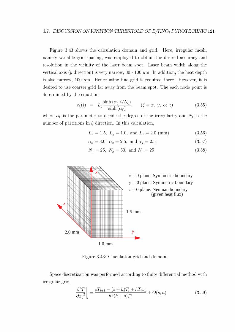
3.7. DISCUSSION ON IGNITION THRESHOLD OF B/KNO3 PYROTECHNIC.121
Figure 3.43 shows the calculation domain and grid. Here, irregular mesh,
namely variable grid spacing, was employed to obtain the desired accuracy and
resolution in the vicinity of the laser beam spot. Laser beam width along the
vertical axis (y direction) is very narrow, 30 - 100 µm. In addition, the heat depth
is also narrow, 100 µm. Hence using fine grid is required there. However, it is
desired to use coarser grid far away from the beam spot. The each node point is
determined by the equation
xξ(i) = Lξsinh (αξ i/Nξ)
sinh (αξ)(ξ = x, y, or z) (3.55)
where αξ is the parameter to decide the degree of the irregularity and Nξ is the
number of partitions in ξ direction. In this calculation,
Lx = 1.5, Ly = 1.0, and Lz = 2.0 (mm) (3.56)
αx = 3.0, αy = 2.5, and αz = 2.5 (3.57)
Nx = 25, Ny = 50, and Nz = 25 (3.58)
x
z
y
1.0 mm
2.0 mm
1.5 mm
z = 0 plane: Neuman boundary (given heat flux)
x = 0 plane: Symmetric boundaryy = 0 plane: Symmetric boundary
Figure 3.43: Claculation grid and domain.
Space discretization was performed according to finite differential method with
irregular grid.
∂2T
∂xξ2
∣∣∣∣∣i
=sTi+1 − (s + h)Ti + hTi−1
hs(h + s)/2+ O(s, h) (3.59)
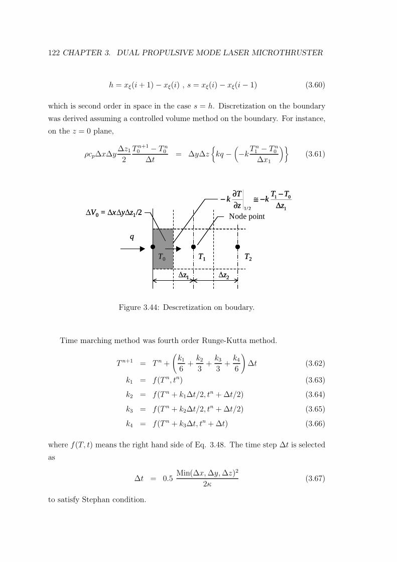
122 CHAPTER 3. DUAL PROPULSIVE MODE LASER MICROTHRUSTER
h = xξ(i + 1) − xξ(i) , s = xξ(i) − xξ(i − 1) (3.60)
which is second order in space in the case s = h. Discretization on the boundary
was derived assuming a controlled volume method on the boundary. For instance,
on the z = 0 plane,
ρcp∆x∆y∆z1
2
T n+10 − T n
0
∆t= ∆y∆z
kq −
(−k
T n1 − T n
0
∆x1
)(3.61)
q
∆V0 = ∆x∆y∆z1/2
T0 T1 T2
∆z1 ∆z2
Node point1
01
2/1 z
TTk
z
Tk
∆−−≅
∂∂−
q
∆V0 = ∆x∆y∆z1/2
T0 T1 T2
∆z1 ∆z2
Node point1
01
2/1 z
TTk
z
Tk
∆−−≅
∂∂−
Figure 3.44: Descretization on boudary.
Time marching method was fourth order Runge-Kutta method.
T n+1 = T n +
(k1
6+
k2
3+
k3
3+
k4
6
)∆t (3.62)
k1 = f(T n, tn) (3.63)
k2 = f(T n + k1∆t/2, tn + ∆t/2) (3.64)
k3 = f(T n + k2∆t/2, tn + ∆t/2) (3.65)
k4 = f(T n + k3∆t, tn + ∆t) (3.66)
where f(T, t) means the right hand side of Eq. 3.48. The time step ∆t is selected
as
∆t = 0.5Min(∆x, ∆y, ∆z)2
2κ(3.67)
to satisfy Stephan condition.
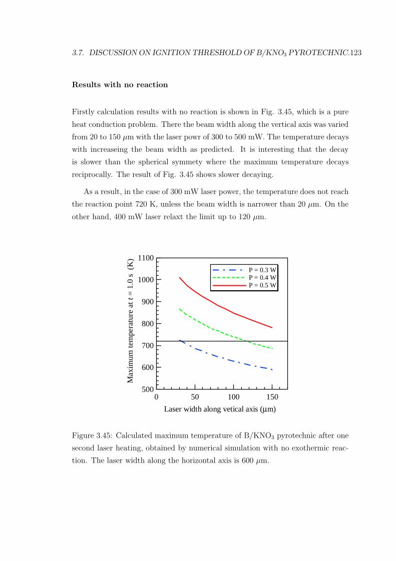
3.7. DISCUSSION ON IGNITION THRESHOLD OF B/KNO3 PYROTECHNIC.123
Results with no reaction
Firstly calculation results with no reaction is shown in Fig. 3.45, which is a pure
heat conduction problem. There the beam width along the vertical axis was varied
from 20 to 150 µm with the laser powr of 300 to 500 mW. The temperature decays
with increaseing the beam width as predicted. It is interesting that the decay
is slower than the spherical symmety where the maximum temperature decays
reciprocally. The result of Fig. 3.45 shows slower decaying.
As a result, in the case of 300 mW laser power, the temperature does not reach
the reaction point 720 K, unless the beam width is narrower than 20 µm. On the
other hand, 400 mW laser relaxt the limit up to 120 µm.
1100
1000
900
800
700
600
500
Max
imum
tem
pera
ture
at t
= 1
.0 s
(K
)
150100500
Laser width along vetical axis (µm)
P = 0.3 W P = 0.4 W P = 0.5 W
Figure 3.45: Calculated maximum temperature of B/KNO3 pyrotechnic after one
second laser heating, obtained by numerical simulation with no exothermic reac-
tion. The laser width along the horizontal axis is 600 µm.

124 CHAPTER 3. DUAL PROPULSIVE MODE LASER MICROTHRUSTER
Estimation of the reaction rate using burning rate
The reaction rate is very important parameter for judging self-sustained combus-
tion of the pyrotechnics. In general, an equation of Arrhenius type
ω(T ) = A exp(− E
RT
)(3.68)
is used to describe the reaction rate [82, 72, 92], where E is the activation energy
and A is a constant. However, it was difficult to obtain actual properties of A and
E and there were no available data for B/KNO3 pyrotechnic.
In this study, a constant reaction rate ωc is estimated using a burning rate
instead of Eq. 3.68. A number of authors have investigated the burning rates of
several pyrotechnics, and also for B/KNO3 [85, 86, 93, 94]. The burning rate vb
and constant reaction rate ωc is related in the steady state combustion as follows.
The governing equation is Eq. 3.48
∂T
∂t= κ
∂2T
∂x2 + ∆TRωs(x, t) (3.69)
∆TR ≡ ∆TR/cp (3.70)
Exothermic reaction of B/KNO3 starts when the temperature reaches to the
threshold TR. The reaction lasts during 1/ωc by the definition of ωc, and the
length of the reaction regime is vb/ωc. The schematic drawing of the system is
shown in Fig. 3.46. In the steady state combustion, putting ξ = x − vbt can be
applied as well as Eq. 3.36, and
−vbdT
dξ= κ
∂2T
∂ξ2 + ∆TRωcs(ξ) (3.71)
s(ξ) =
⎧⎨⎩ 0 , vb/ωc < ξ
1 , 0 < ξ < vb/ωc
(3.72)
B.C. T (∞) = T∞,dT
dξ
∣∣∣∣∣0
=ρ∆hPTv
k, T (vb/ωc) = TR (3.73)
Moving ξ frame was taken to have the reaction regime 0 < ξ < vb/ωc. In the region
of ξ > vb/ωc, B/KNO3 is simply heated with maintaining T = TR at ξ = vb/ωc.
At the ξ = 0 surface, KNO3 decomposes to gas, which needs positive temperature
gradient corresponding to the heat of phase transformation (decomposition). In
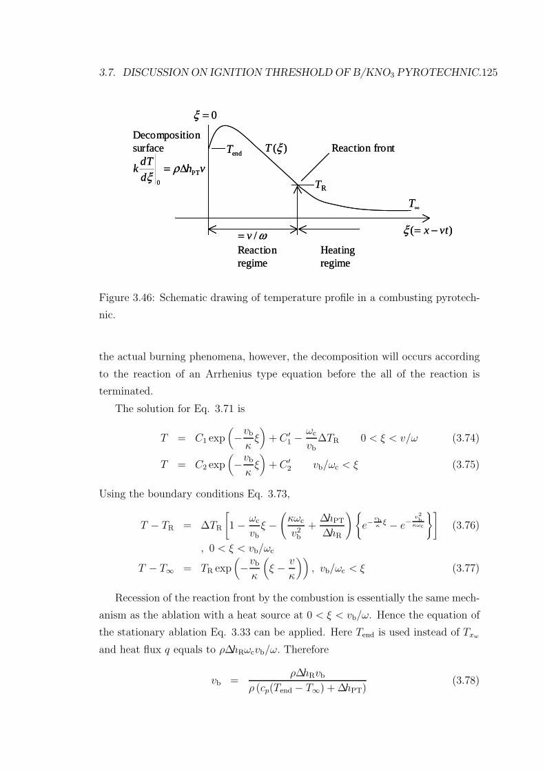
3.7. DISCUSSION ON IGNITION THRESHOLD OF B/KNO3 PYROTECHNIC.125
)(ξT
)( vtx −=ξ
TR
Heating regime
Reaction regime
ω/v=
Reaction front
∞T
endTDecomposition surface
0=ξ
vhd
dTk PT
0
∆= ρξ
)(ξT
)( vtx −=ξ
TR
Heating regime
Reaction regime
ω/v=
Reaction front
∞T
endTDecomposition surface
0=ξ
vhd
dTk PT
0
∆= ρξ
Figure 3.46: Schematic drawing of temperature profile in a combusting pyrotech-
nic.
the actual burning phenomena, however, the decomposition will occurs according
to the reaction of an Arrhenius type equation before the all of the reaction is
terminated.
The solution for Eq. 3.71 is
T = C1 exp(−vb
κξ)
+ C ′1 −
ωc
vb∆TR 0 < ξ < v/ω (3.74)
T = C2 exp(−vb
κξ)
+ C ′2 vb/ωc < ξ (3.75)
Using the boundary conditions Eq. 3.73,
T − TR = ∆TR
[1 − ωc
vb
ξ −(
κωc
v2b
+∆hPT
∆hR
)e−
vbκ
ξ − e−v2b
κωc
](3.76)
, 0 < ξ < vb/ωc
T − T∞ = TR exp(−vb
κ
(ξ − v
κ
)), vb/ωc < ξ (3.77)
Recession of the reaction front by the combustion is essentially the same mech-
anism as the ablation with a heat source at 0 < ξ < vb/ω. Hence the equation of
the stationary ablation Eq. 3.33 can be applied. Here Tend is used instead of Txw
and heat flux q equals to ρ∆hRωcvb/ω. Therefore
vb =ρ∆hRvb
ρ (cp(Tend − T∞) + ∆hPT)(3.78)
126 CHAPTER 3. DUAL PROPULSIVE MODE LASER MICROTHRUSTER
∆hR = cp(Tend − T∞) + ∆hPT (3.79)
Putting ξ = 0 into Eq. 3.76,(ωκ
v2+
∆hPT
∆hR
)(1 − exp
(− v2
ωκ
))=
cp(TR − T∞) + ∆hPT
∆hR(3.80)
Solving Eq. 3.80 for ωc, the reaction rate can be expressed as a function of vR.
However, that solution can not be expressed by an algebraic way. Fortunately, in
the most cases of pyrotechnic combustion, v2b/ωcκ is much larger than one and the
exponential term in the left hand side of Eq.3.80 can be neglected. In that case,
the reaction rate is simply related to the burning rate as
ωc =cp(TR − T∞)
∆hR
v2b
κ(3.81)
The boron/potassium nitrate pellet used in this study is supplied from Nichiyu
Giken Kogyo CO., LTD. It contains 30 % boron particle by the weight fraction.
The diameters of the particles are less than 1.0 µm. They have the data on the
burning rate of
vb (mm/s) = 24 p0.08 , (5 < p < 50kg/cm2) (3.82)
The low pressure exponent of 0.08 means very weak dependence of the burning
rate on the pressure as expected above. Whereas that rate is for higher pressure
than the atmosphere and not for low pressure environment like this study, the
burning rate of 24 mm/s is used. Using the properties in Table 3.11, the constant
reaction rate is obtained as
ωc = 97 (1/s) (3.83)
It should be noted that that reaction rate can contain large error, because the
reaction rate is quadratically affected by the burning rate. Additionally, in several
studies measuring the burning rate of B/KNO3, other values were measured at 30
% weight fraction and 0.1 MPa, 10 mm/s [85], 25 mm/s [93], and 10 mm/s [94].
In the case of 10 mm/s the burning rate, the reaction rate becomes one fifth, 16
1/s. The difference would be caused by particle size and environment conditions.
In the calculation, the reaction rate was changed from 10 to 130 /s to check the
dependence.
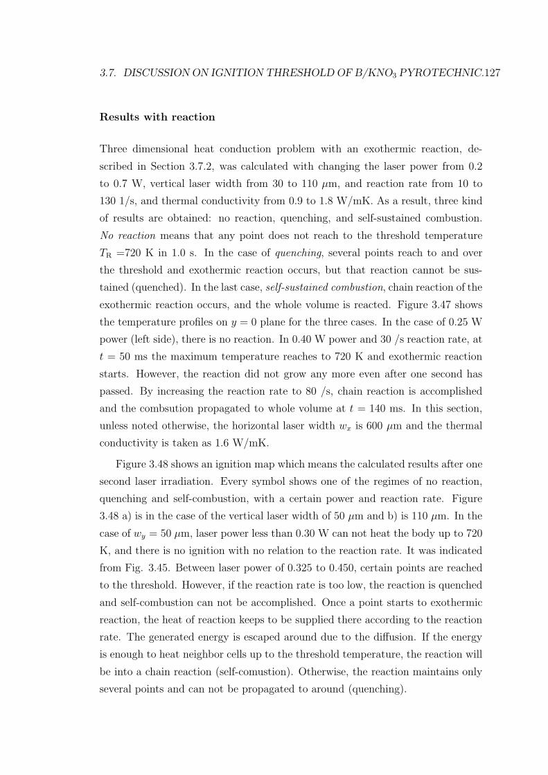
3.7. DISCUSSION ON IGNITION THRESHOLD OF B/KNO3 PYROTECHNIC.127
Results with reaction
Three dimensional heat conduction problem with an exothermic reaction, de-
scribed in Section 3.7.2, was calculated with changing the laser power from 0.2
to 0.7 W, vertical laser width from 30 to 110 µm, and reaction rate from 10 to
130 1/s, and thermal conductivity from 0.9 to 1.8 W/mK. As a result, three kind
of results are obtained: no reaction, quenching, and self-sustained combustion.
No reaction means that any point does not reach to the threshold temperature
TR =720 K in 1.0 s. In the case of quenching, several points reach to and over
the threshold and exothermic reaction occurs, but that reaction cannot be sus-
tained (quenched). In the last case, self-sustained combustion, chain reaction of the
exothermic reaction occurs, and the whole volume is reacted. Figure 3.47 shows
the temperature profiles on y = 0 plane for the three cases. In the case of 0.25 W
power (left side), there is no reaction. In 0.40 W power and 30 /s reaction rate, at
t = 50 ms the maximum temperature reaches to 720 K and exothermic reaction
starts. However, the reaction did not grow any more even after one second has
passed. By increasing the reaction rate to 80 /s, chain reaction is accomplished
and the combsution propagated to whole volume at t = 140 ms. In this section,
unless noted otherwise, the horizontal laser width wx is 600 µm and the thermal
conductivity is taken as 1.6 W/mK.
Figure 3.48 shows an ignition map which means the calculated results after one
second laser irradiation. Every symbol shows one of the regimes of no reaction,
quenching and self-combustion, with a certain power and reaction rate. Figure
3.48 a) is in the case of the vertical laser width of 50 µm and b) is 110 µm. In the
case of wy = 50 µm, laser power less than 0.30 W can not heat the body up to 720
K, and there is no ignition with no relation to the reaction rate. It was indicated
from Fig. 3.45. Between laser power of 0.325 to 0.450, certain points are reached
to the threshold. However, if the reaction rate is too low, the reaction is quenched
and self-combustion can not be accomplished. Once a point starts to exothermic
reaction, the heat of reaction keeps to be supplied there according to the reaction
rate. The generated energy is escaped around due to the diffusion. If the energy
is enough to heat neighbor cells up to the threshold temperature, the reaction will
be into a chain reaction (self-comustion). Otherwise, the reaction maintains only
several points and can not be propagated to around (quenching).
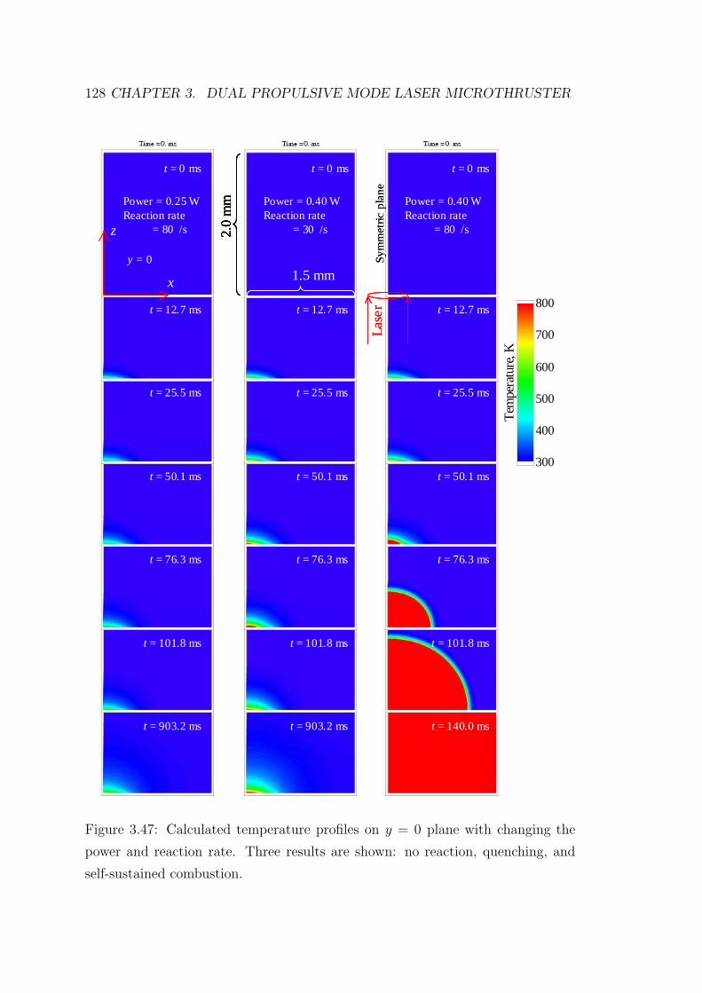
128 CHAPTER 3. DUAL PROPULSIVE MODE LASER MICROTHRUSTER
erutarepme
T,K
300
400
500
600
700
800
t = 0 ms
t = 50.1 ms
t = 25.5 ms
t = 12.7 ms
t = 101.8 ms
t = 76.3 ms
t = 903.2 ms
z
x
Power = 0.25 WReaction rate
= 80 /s
t = 0 ms
t = 50.1 ms
t = 25.5 ms
t = 12.7 ms
t = 101.8 ms
t = 76.3 ms
t = 903.2 ms
2.0
mm
1.5 mm
Power = 0.40 WReaction rate
= 30 /s
t = 0 ms
t = 50.1 ms
t = 25.5 ms
t = 12.7 ms
t = 101.8 ms
t = 76.3 ms
t = 140.0 ms
Power = 0.40 WReaction rate
= 80 /s
y = 0
Las
erSy
mm
etric
pla
ne
erutarepme
T,K
300
400
500
600
700
800
t = 0 ms
t = 50.1 ms
t = 25.5 ms
t = 12.7 ms
t = 101.8 ms
t = 76.3 ms
t = 903.2 ms
z
x
Power = 0.25 WReaction rate
= 80 /s
t = 0 ms
t = 50.1 ms
t = 25.5 ms
t = 12.7 ms
t = 101.8 ms
t = 76.3 ms
t = 903.2 ms
z
x
Power = 0.25 WReaction rate
= 80 /s
t = 0 ms
t = 50.1 ms
t = 25.5 ms
t = 12.7 ms
t = 101.8 ms
t = 76.3 ms
t = 903.2 ms
2.0
mm
1.5 mm
Power = 0.40 WReaction rate
= 30 /s
t = 0 ms
t = 50.1 ms
t = 25.5 ms
t = 12.7 ms
t = 101.8 ms
t = 76.3 ms
t = 903.2 ms
2.0
mm
1.5 mm
Power = 0.40 WReaction rate
= 30 /s
t = 0 ms
t = 50.1 ms
t = 25.5 ms
t = 12.7 ms
t = 101.8 ms
t = 76.3 ms
t = 140.0 ms
Power = 0.40 WReaction rate
= 80 /s
t = 0 ms
t = 50.1 ms
t = 25.5 ms
t = 12.7 ms
t = 101.8 ms
t = 76.3 ms
t = 140.0 ms
Power = 0.40 WReaction rate
= 80 /s
y = 0
Las
erSy
mm
etric
pla
ne
Figure 3.47: Calculated temperature profiles on y = 0 plane with changing the
power and reaction rate. Three results are shown: no reaction, quenching, and
self-sustained combustion.
3.7. DISCUSSION ON IGNITION THRESHOLD OF B/KNO3 PYROTECHNIC.129
0
50
100
0 0.2 0.4 0.6
Power (W)
Rea
ctio
n ra
te (
1/s)
Ignition
Quench
No reaction
a)
0
50
100
0 0.2 0.4 0.6
Power (W)
Rea
ctio
n ra
te (
1/s)
Ignition
Quench
No reaction
b)
Figure 3.48: Mapping of the calculated result: ignition, quench, or no-reaction,
a)Wy =50 µm and b)Wy =110 µm.
130 CHAPTER 3. DUAL PROPULSIVE MODE LASER MICROTHRUSTER
The wider is laser width, the more power is required to heat up to the threshold
temperature. Hence, in the case of wy =110 µm, at least 0.4 W is necessary to
starts the reaction. However, once the reaction starts, it is easier for the combus-
tion surface to propagate around than narrow laser width, because the area which
reacts at a time is larger.
The reaction rate of our B/KNO3 was estimated as about 100 /s in the above
section. That value gives the threshold laser power of 0.35 W for wy =50 µm
and 0.4 W wy =110 µm. It well agreed with the experimental results of ignition
probability measurement (Fig. 3.33). In that experiment, we could not know the
accurate vertical laser width of the laser, because it was difficult to accurately set
the pyrotechnic for laser. The associated position error would be less than ± 0.5
mm, and it causes the inaccuracy of laser width from 50 to 110 µm. However, it is
shown by the calculation that the threshold power is changed only 0.05 W. even
if the width is changed from 50 to 110 µm
The calculation conducted here has another uncertainty, the thermal conduc-
tivity. In the above calculation, the conductivity is taken as 1.6 W/mK. Whereas
that value is calculated according to the empirical equation, there are other pre-
dictive equation and there are large variation of those, as shown in Appendix D. In
addition, the conductivity of boron decreased with the increase of the temperature
(1.6 W/mK is calculated using one at 400 K). Then to confirm the effect of the
conductivity, the threshold power was compared between 1.6 and 1.2 W/mK in
Fig. 3.49. Figure 3.49 a) is the case of the thermal conductivity of 1.6 W/mK
and b) is 1.2 W/mK. It is shown that decreasing thermal conductivity decreases
the threshold power, which is within 0.25 to 0.33 W in the reaction rate around
100 1/s. That value is closer to the experimental results than at 1.6 W/mK.
Another quantitative evaluation of the calculation code was carried out by
comparing the ignition time. As an index to evaluate the ignition time, the reactive
fraction µce is defined as
µce(t) ≡
∫V
∫ t
0ρ∆hRωRs(t, x) dt dx
ρ∆hRV(3.84)
where the denominator means the total chemical energy included in the system
(pellet) and the numerator is the chemical energy released in the time t. Figure
3.50 shows the time when the reactive fraction reaches to 55 %. Figure 3.50 a)
3.7. DISCUSSION ON IGNITION THRESHOLD OF B/KNO3 PYROTECHNIC.131
0.60
0.50
0.40
0.30
0.20
0.10
0.00
Thr
esho
ld p
ower
(W
)
150100500
Reaction rate (/s)
wy = 30 µm
wy = 50 µm
wy = 70 µm
wy = 110 µm
a)
0.60
0.50
0.40
0.30
0.20
0.10
0.00
Thr
esho
ld p
ower
(W
)
150100500
Reaction rate (/s)
wy = 30 µm
wy = 50 µm
wy = 70 µm
wy = 110 µm
b)
Figure 3.49: Claculated threshold power for the laser ignition of B/KNO3 py-
rotechnic, a)k =1.6 W/mK and b)k =1.2 W/mK.

132 CHAPTER 3. DUAL PROPULSIVE MODE LASER MICROTHRUSTER
is in the case of wy = 50 µm and b) is wy = 110 µm. As the laser power goes
close to the threshold power, the ignition time is drastically extended. With the
enough laser power, the ignition times are ranged from 150 to 350 ms according
to the reaction rate. Reaction rate more than 40 /s gives the ignition time around
200 ms. That value almost agrees with the experimentally observed combustion
pictures, although it was difficult to precisely determin the ignition time in the
experiment.
3.7. DISCUSSION ON IGNITION THRESHOLD OF B/KNO3 PYROTECHNIC.133
0.60
0.50
0.40
0.30
0.20
0.10
0.00
Igni
tion
tim
e (s
)
0.80.60.40.20.0
Laser power (W)
Reaction rate = 20 /s Reaction rate = 40 /s Reaction rate = 60 /s Reaction rate = 80 /s Reaction rate = 100 /s
a)
0.60
0.50
0.40
0.30
0.20
0.10
0.00
Igni
tion
tim
e (s
)
0.80.60.40.20.0
Laser power (W)
Reaction rate = 20 /s Reaction rate = 40 /s Reaction rate = 60 /s Reaction rate = 80 /s Reaction rate = 100 /s
b)
Figure 3.50: Claculated ignition time when 55 % of volume starts the reaction
(k =1.6 W/mK), a)Wy =50 µm and b)Wy =110 µm.
134 CHAPTER 3. DUAL PROPULSIVE MODE LASER MICROTHRUSTER
3.8 Conclusion of Chapter 3
In this chapter, a dual propulsive mode laser microthruster was proposed and
developed, and the following conclusions were obtained.
• Successful operations of the laser ablation mode was verified using polyvinyl
chloride propellant. The thrust provided by the laser ablation was propor-
tional to the laser pulse width. The thrust to power ratio ranged from 40 to
150 µNs/J correspoing to the ablative material. Therefore the laser ablation
mode provides widely ranged thrust with arbitrary resolution by selecting
the ablative material suited with the required thrust resolution.
• Absorption rate of the ablative propellant strongly affected the thrust per-
formance, especially thrust to power ratio. Polyvinyl chloride with rich car-
bon density showed higher thrust to power ratio. The ablation of PVC by
one Watts class diode laser was caused by teh dehydrochlorination, and the
degradation of HCl can be explained by the photothermal reaction.
• Boron / potassium nitrate pyrotechnics is suited with laser igntion in vac-
uum, and it was experimentally verified. The threshold laser power and pulse
with for the laser ignition was adequate for the use of microspacecraft, 300
mW and 150 ms. Composite propellant and double-base propellant was not
ignited by 1 W diode laser in vacuum. The laser ignition processes of Boron
/ potassium nitrate was well reproduced with numerical calculation, where
three dimensional heat conduction problem was solved with the exothermic
reaction.
• That laser ignited combustion provided thrust of 11 mNs when using a 30
mg pyrotechnic and thrust of 600 mNs when using a 1.0 mg pyrotechnic.
Those much higher thrust than laser ablation thrusters covers wide range of
thrust by combining laser ablation, and it enables a single micropropulsion
conducting multiple propulsion tasks.
Chapter 4
Liquid Propellant Pulsed Plasma
Thruster
4.1 Introduction
4.1.1 Pulsed plasma thrusters
In recent years, Pulsed Plasma Thrusters (PPTs) have attracted great attention
as promising thrusters for microspacecraft. They have compat size suitable with
microspacecraft and provide high specific impulse of the order of 1000 s. In stead
of the high specific impulse, however, PPTs require a energy storing capacitor
and power processing unit (PPU) charging it. Typically ten Joules class PPTs
requires weight of 0.2 to 1.0 kg for the capacitor and PPU. Therefore the adequate
spacecraft size for PPTs are larger than ones dealt in the previous chapter. That
size would be over 10 kg. For instance, a 10-50 J class PPT installed on the Earth
Observing 1 (EO-1) spacecraft weighs 4.95 kg with two thruster heads, a common
capacitor, and a single power processing unit [95]. A bread-boad model PPT with
1-5 J class, which was developed in Tokyo Metroporitan Institure of Technology,
weighs less than 2.0 kg [96]. It has also have two heads, a common capacitor, and
single PPU.
A PPT is a pulsed electric propulsion, and can be operated in low power levels
of 1 to 100 W, whereas most electric propulsions require high power levels over a
few 100 W. Power throttling of PPTs is managed simply by changing the pulse
repetition frequency. That throttling does not affect the performance because the
135
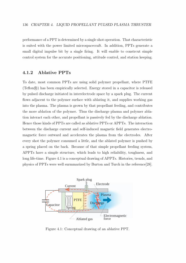
136 CHAPTER 4. LIQUID PROPELLANT PULSED PLASMA THRUSTER
performance of a PPT is determined by a single shot operation. That characteristic
is suited with the power limited microspacecraft. In addition, PPTs generate a
small digital impulse bit by a single firing. It will enable to constrcut simple
control system for the accurate positioning, attitude control, and station keeping.
4.1.2 Ablative PPTs
To date, most common PPTs are using solid polymer propellant, where PTFE
(Teflon r©) has been empirically selected. Energy stored in a capacitor is released
by pulsed discharge initiated in interelectrode space by a spark plug. The current
flows adjacent to the polymer surface with ablating it, and supplies working gas
into the plasma. The plasma is grown by that propellant feeding, and contributes
the more ablation of the polymer. Thus the discharge plasma and polymer abla-
tion interact each other, and propellant is passively fed by the discharge ablation.
Hence those kinds of PPTs are called as ablative PPTs or APPTs. The interaction
between the discharge current and self-induced magnetic field generates electro-
magnetic force outward and accelerates the plasma from the electrodes. After
every shot the polymer consumed a little, and the ablated polymer is pushed by
a spring placed on the back. Because of that simple propellant feeding system,
APPTs have a simple structure, which leads to high reliability, toughness, and
long life-time. Figure 4.1 is a conceptual drawing of APPTs. Histories, trends, and
physics of PPTs were well surmmarized by Burton and Turch in the reference[28].
Spark plug
Capacitor
Current
Spring
PTFE
Ablated gas
Plasma
Electromagnetic force
Electrode
Discharge
Figure 4.1: Conceptual drawing of an ablative PPT.
4.1. INTRODUCTION 137
However, there are several problems on ablative PPTs: poor thrust perfor-
mance, contamination, and non-uniform ablation. To improve the performance
of APPTs, various studies have been performed. Nevertheless, flight-qualified
APPTs have been still remained in the efficiency of less than 10 % [97, 95, 96].
Several researchers in this field have pointed out that the excessive propellant
feeding after the main discharge causes the low performance. It was observed
that low speed vapor continues to be provided after the main discharge [98, 99]. It
would be because the surface temperature remains higher than the boiling point of
the propellant. Additionally the emission of large particulates was observed [100],
which could not be effectively accelerated. Such kinds of low speed propellants
hardly contribute to the thrust and decrease the propellant utilization efficiency.
In order to improve the propellant efficiency, it is necessary to supply only an
minimum amount of propellant for both ionization and acceleration.
Contamination problems on spacecraft or thruster itself is caused by the ex-
haust plasma gas of PTFE. PTFE is made of carbon and fluorine. The reason
why PTFE was selected of a number of polymers was the charring[101], that is,
alternative propellants failed due to the severe carbonization. In the early work
on PPTs, carbonization on a spark plug was studied [102], which eventually failed
the operation. In these days, failure reports due to charring has not been known,
and Myers and Arrington reported that the contamination did not affect on space-
craft [103]. However, contamination issues always remain as potential with using
PTFE, especially for applications with highly sensitive diagnostics for ineterfer-
ometry missions.
The non-uniform ablation is caused by the profiles of the current density and
PTFE surface temperature. There are preferential ablations near the electrodes
[104]. Such non-uniform ablation varies the impulse bit trend in successive op-
eration and decreases the amount of usable propellant. That phenomena was
remarkable for the small energy levels and small size [96, 105].
After all, the several disadvantages have made scientists hesitate to apply PPTs
in spacecraft, whereas PPTs would be only one thruster in electric propulsions
applicable to microspacecraft due to their compactness, low power operation, and
useful digital impulse. Therefore studies on high performance and contamination
free PPTs are very important and such thrusters will be promising micropropulsion
providing high delta-v.
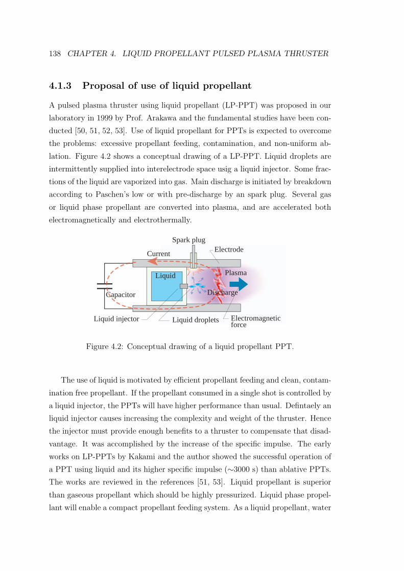
138 CHAPTER 4. LIQUID PROPELLANT PULSED PLASMA THRUSTER
4.1.3 Proposal of use of liquid propellant
A pulsed plasma thruster using liquid propellant (LP-PPT) was proposed in our
laboratory in 1999 by Prof. Arakawa and the fundamental studies have been con-
ducted [50, 51, 52, 53]. Use of liquid propellant for PPTs is expected to overcome
the problems: excessive propellant feeding, contamination, and non-uniform ab-
lation. Figure 4.2 shows a conceptual drawing of a LP-PPT. Liquid droplets are
intermittently supplied into interelectrode space usig a liquid injector. Some frac-
tions of the liquid are vaporized into gas. Main discharge is initiated by breakdown
according to Paschen’s low or with pre-discharge by an spark plug. Several gas
or liquid phase propellant are converted into plasma, and are accelerated both
electromagnetically and electrothermally.
Spark plug
Capacitor
Current
Plasma
Electromagnetic force
Electrode
Discharge
Liquid
Liquid dropletsLiquid injector
Figure 4.2: Conceptual drawing of a liquid propellant PPT.
The use of liquid is motivated by efficient propellant feeding and clean, contam-
ination free propellant. If the propellant consumed in a single shot is controlled by
a liquid injector, the PPTs will have higher performance than usual. Defintaely an
liquid injector causes increasing the complexity and weight of the thruster. Hence
the injector must provide enough benefits to a thruster to compensate that disad-
vantage. It was accomplished by the increase of the specific impulse. The early
works on LP-PPTs by Kakami and the author showed the successful operation of
a PPT using liquid and its higher specific impulse (∼3000 s) than ablative PPTs.
The works are reviewed in the references [51, 53]. Liquid propellant is superior
than gaseous propellant which should be highly pressurized. Liquid phase propel-
lant will enable a compact propellant feeding system. As a liquid propellant, water
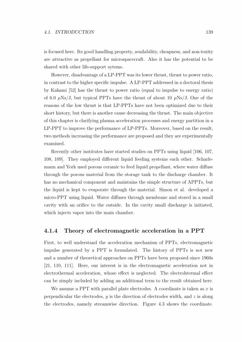
4.1. INTRODUCTION 139
is focused here. Its good handling property, availability, cheapness, and non-toxity
are attractive as propellant for microspacecraft. Also it has the potential to be
shared with other life-support sytems.
However, disadvantage of a LP-PPT was its lower thrust, thrust to power ratio,
in contrast to the higher specific impulse. A LP-PPT addressed in a doctoral thesis
by Kakami [52] has the thrust to power ratio (equal to impulse to energy ratio)
of 6.0 µNs/J, but typical PPTs have the thrust of about 10 µNs/J. One of the
reasons of the low thrust is that LP-PPTs have not been optimized due to their
short history, but there is another cause decreasing the thrust. The main objective
of this chapter is clarifying plasma acceleration processes and energy partition in a
LP-PPT to improve the performance of LP-PPTs. Moreover, based on the result,
two methods increasing the performance are proposed and they are experimentally
examined.
Recently other institutes have started studies on PPTs using liquid [106, 107,
108, 109]. They employed different liquid feeding systems each other. Scharle-
mann and York used porous ceramic to feed liquid propellant, where water diffuse
through the porous material from the storage tank to the discharge chamber. It
has no mechanical component and maintains the simple structure of APPTs, but
the liquid is kept to evaporate through the material. Simon et al. developed a
micro-PPT using liquid. Water diffuses through membrane and stored in a small
cavity with an orifice to the outside. In the cavity small discharge is initiated,
which injects vapor into the main chamber.
4.1.4 Theory of electromagnetic acceleration in a PPT
First, to well understand the acceleration mechanism of PPTs, electromagnetic
impulse generated by a PPT is formulated. The history of PPTs is not new
and a number of theoretical approaches on PPTs have been proposed since 1960s
[21, 110, 111]. Here, our interest is in the electromagnetic acceleration not in
electrothermal acceleration, whose effect is neglected. The electrohtermal effect
can be simply included by adding an additional term to the result obtained here.
We assume a PPT with parallel plate electrodes. A coordinate is taken as x is
perpendicular the electrodes, y is the direction of electrodes width, and z is along
the electrodes, namely streamwise direction. Figure 4.3 shows the coordinate.
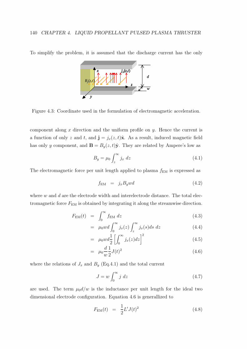
140 CHAPTER 4. LIQUID PROPELLANT PULSED PLASMA THRUSTER
To simplify the problem, it is assumed that the discharge current has the only
x
y
z
jx(z,t)
By(z,t)
w
d
x
y
z
jx(z,t)
By(z,t)
x
y
z
jx(z,t)
By(z,t)
w
d
Figure 4.3: Coordinate used in the formulation of electromagnetic acceleration.
component along x direction and the uniform profile on y. Hence the current is
a function of only z and t, and j = jx(z, t)x. As a result, induced magnetic field
has only y component, and B = By(z, t)y. They are related by Ampere’s low as
By = µ0
∫ ∞
zjx dz (4.1)
The electromagnetic force per unit length applied to plasma fEM is expressed as
fEM = jxBywd (4.2)
where w and d are the electrode width and interelectrode distance. The total elec-
tromagnetic force FEM is obtained by integrating it along the streamwise direction.
FEM(t) =∫ ∞
0fEM dz (4.3)
= µ0wd∫ ∞
0jx(z)
∫ ∞
zjx(s)ds dz (4.4)
= µ0wd1
2
[∫ ∞
0jx(z)dz
]2(4.5)
= µ0d
w
1
2J(t)2 (4.6)
where the relations of Jx and By (Eq.4.1) and the total current
J = w∫ ∞
0j dz (4.7)
are used. The term µ0d/w is the inductance per unit length for the ideal two
dimensional electrode configuration. Equation 4.6 is generallized to
FEM(t) =1
2L′J(t)2 (4.8)
4.1. INTRODUCTION 141
using the inductance per unit length L′. As a result, the squared discharge current
and the inductance per unit lenght of the electrode are essential parameters of
electromagnetic acceleration.
The power consumed for the electromagnetic acceleration WEM is
WEM =∫ ∞
0u(z, t)fEM(z, t) dz (4.9)
v(t)∫ ∞
0fEM(z, t) dz =
1
2L′v(t)J(t)2 (4.10)
where u(z, t) is the fluid velocity of the plasma and v(t) is the characteristic velocity
over the electrode, which is defined as
v(t) ≡∫ ∞
0u(z, t)fEM(z, t) dz
/∫ ∞
0fEM(z, t) dz (4.11)
The work done on the moving plasma by the electromagnetic force during the
pulsed discharge is
EEM =∫ ∞
0
1
2L′v(t)J(t)2 dt (4.12)
The term 12L′v(t) in the integral has the same unit as the resistance, and it is re-
ferred as the equivalent resistance of electromagnetic acceleration, and abbreviated
to REM.
REM(t) ≡ 1
2L′v(t) (4.13)
The energy initially stored in the capacitor of the PPT, E0, is consumed as
the electromagnetic work or as the dissipation at the resistance of the plasma
Rplasma and the resistance of an external circuit Rcircuit. Here the external circuit
means the capacitor and feed lines from electrodes, and Rcircuit includes all of those
resistances. Of course, the energy dissipated in the external circuit is hardly used
for the acceleration and it becomes energy loss. Expressing the relation of the
energy and those resistances,
E0 =∫ ∞
0
(Rcircuit + Rplasma(t) +
1
2L′v(t)
)J(t)2 dt (4.14)
=(Rcircuit + Rplasma +
1
2L′v) ∫ ∞
0J(t)2 dt (4.15)
where Rplasma and REM are averaged resistances of plasma and electromagnetic
work, defined by
Rplasma ≡∫ ∞
0Rplasma(t)J
2 dt/∫ ∞
0J2 dt (4.16)
142 CHAPTER 4. LIQUID PROPELLANT PULSED PLASMA THRUSTER
REM ≡ 1
2L′v (4.17)
v ≡∫ ∞
0v(t)J 2 dt
/∫ ∞
0J2 dt (4.18)
=∑n
∫nth1/2cycle
vnJ2 dt
/∫ ∞
0J2 dt (4.19)
Here let us define the effective resistance of the plasma R∗plasma and the total
resistance of the PPT circuit Rtotal as
R∗plasma ≡ Rplasma + REM (4.20)
Rtotal ≡ Rcircuit + Rplasma + REM (4.21)
When the energy conversion efficiency is defined as the fraction of the work done
by the electromagnetic force to the initial stored energy, it is expressed as
ηEM =REM
Rtotal(4.22)
The impulse that the thruster generates (the momentum given to the plasma) is
expressed as by using Eqs. 4.8, 4.15, and 4.21,
IEM =∫ ∞
0FEM dt =
1
2L′∫ ∞
0J(t)2 dt (4.23)
1
2L′ E0
Rtotal(4.24)
Therefore it is very important to know the resistances of Rcircuit, Rplasma, and
REM. They determines the energy efficiency (or energy partition) and the thrust
to power ratio. Therefore those resistances are estimated in the succeeding sec-
tions. The total resistance of the PPT circuit Rtotal is easily calculated using
initially stored energy and integral of the squared discharge current according to
Eq. 4.15. The Rcircuit is obtained from the discharge without plasma described in
the succeeding section. The equivalent resistance of the electromagnetic work REM
cannot be obtained unless the characteristic velocity of the plasma is calculated
according to Eq. 4.11. That velocity is roughly obtained using pictures taken by
ultra high-speed camera.
4.2. EXPERIMENTAL SETUP 143
4.2 Experimental setup
4.2.1 Vacuum facilities
Experiments on pulsed plasma thrusters were conducted in a 1.1-m-diam, 1.8-m-
long vacuum chamber, UT cylindrical chamber. It is the same chamber used for
experiments on the laser ablation. The background pressures were maintained
under 1 − 5 × 10⁻⁵ Torr. The inner pressure was measured using a ionization
vacuum gauge. The detailed explanation is described in Appendix B.
The space chamber was electrically connected to the ground due to prevent
the possibility charging up to high voltage for the safety. However, the potential
of the chamber was instantaneously pulled up and down by the pulsed discharge
of PPTs (with a few hundred volts amplitude). It affected the base potential of
an oscilloscope and disturbed the measured waveforms of current and voltage. To
reduce the effect, the ground line of the oscilloscope used was directly connected
to the chamber wall.
4.2.2 Liquid injector
A liquid propellant PPT proposed here requires an intermediate injector to supply
liquid in vacuum. The injector should have small and light body to be suited with
microspacecraft. In addition the injector must supply very minute liquid a shot,
because mass shot required for 10 W class PPTs are very small, a few micro grams.
In the study of liquid propellant PPTs, development of such a liquid injector is
most important and it will become a key technology to determine the performance.
Ink-jet type injector
In the early stage of this study, we attempted to apply the ink-jet technology in
printers into the injector of a LP-PPT. Ink-jet printers inject liquid droplets from
a small pinhole with the pressure increase by a piezoelectric device or film boiling
of small bubble in the tank. It has no shut off valve and seals liquid by the surface
tension. It leads to a simple and compact structure, and supplies a extremely
small amount of droplets, of pico-little. Those characters are also suitable with an
injector expected for a liquid propellant PPT.
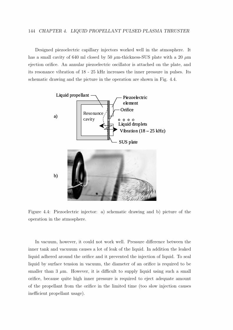
144 CHAPTER 4. LIQUID PROPELLANT PULSED PLASMA THRUSTER
Designed piezoelectric capillary injectors worked well in the atmosphere. It
has a small cavity of 640 ml closed by 50 µm-thickness-SUS plate with a 20 µm
ejection orifice. An annular piezoelectric oscillator is attached on the plate, and
its resonance vibration of 18 - 25 kHz increases the inner pressure in pulses. Its
schematic drawing and the picture in the operation are shown in Fig. 4.4.
Liquid droplets
Liquid propellant Piezoelectric element
SUS plate
Resonance cavity
Vibration (18 – 25 kHz)
Orificea)
b)
Liquid droplets
Liquid propellant Piezoelectric element
SUS plate
Resonance cavity
Vibration (18 – 25 kHz)
Orificea)
b)
Figure 4.4: Piezoelectric injector: a) schematic drawing and b) picture of the
operation in the atmosphere.
In vacuum, however, it could not work well. Pressure difference between the
inner tank and vacuuum causes a lot of leak of the liquid. In addition the leaked
liquid adhered around the orifice and it prevented the injection of liquid. To seal
liquid by surface tension in vacuum, the diameter of an orifice is required to be
smaller than 3 µm. However, it is difficult to supply liquid using such a small
orifice, because quite high inner pressure is required to eject adequate amount
of the propellant from the orifice in the limited time (too slow injection causes
inefficient propellant usage).
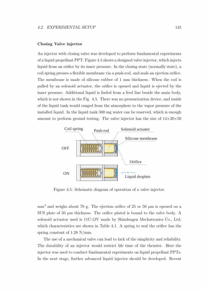
4.2. EXPERIMENTAL SETUP 145
Closing Valve injector
An injector with closing valve was developed to perform fundamental experiments
of a liquid propellant PPT. Figure 4.5 shows a designed valve injector, which injects
liquid from an orifice by its inner pressure. In the closing state (normally state), a
coil spring presses a flexible membrane via a push-rod, and seals an ejection orifice.
The membrane is made of silicone rubber of 1 mm thickness. When the rod is
pulled by an solenoid actuator, the orifice is opened and liquid is ejected by the
inner pressure. Additional liquid is fueled from a feed line beside the main body,
which is not shown in the Fig. 4.5. There was no pressurization device, and inside
of the liquid tank would ranged from the atmosphere to the vapor pressure of the
installed liquid. In the liquid tank 500 mg water can be reserved, which is enough
amount to perform ground testing. The valve injector has the size of 14×20×50
Orifice
Solenoid actuater
Liquid dropletsON
OFF
Coil spring Push-rod
Silicone membrane
Figure 4.5: Schematic diagram of operation of a valve injector.
mm3 and weighs about 78 g. The ejection orifice of 25 or 50 µm is opened on a
SUS plate of 50 µm thickness. The orifice plated is bound to the valve body. A
solenoid actuator used is 11C-12V made by Shindengen Mechatronics Co., Ltd,
which characteristics are shown in Table 4.1. A spring to seal the orifice has the
spring constant of 1.28 N/mm.
The use of a mechanical valve can lead to lack of the simplicity and reliability.
The durability of an injector would restrict life time of the thruster. Here the
injector was used to conduct fundamental experiments on liquid propellant PPTs.
In the next stage, further advanced liquid injector should be developed. Recent
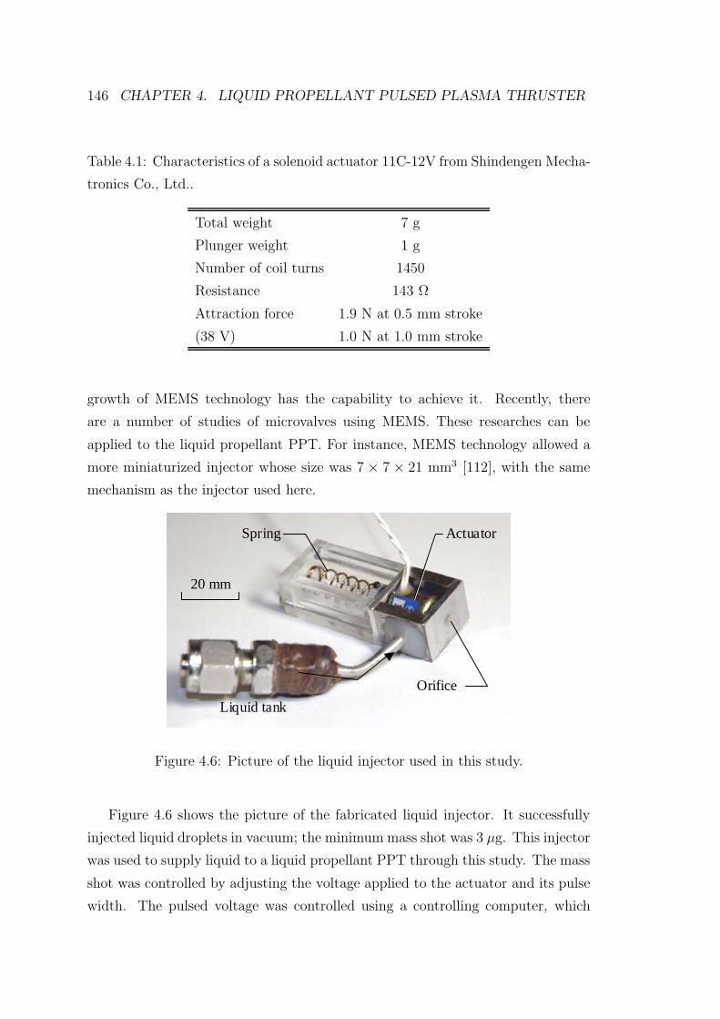
146 CHAPTER 4. LIQUID PROPELLANT PULSED PLASMA THRUSTER
Table 4.1: Characteristics of a solenoid actuator 11C-12V from Shindengen Mecha-
tronics Co., Ltd..
Total weight 7 g
Plunger weight 1 g
Number of coil turns 1450
Resistance 143 Ω
Attraction force 1.9 N at 0.5 mm stroke
(38 V) 1.0 N at 1.0 mm stroke
growth of MEMS technology has the capability to achieve it. Recently, there
are a number of studies of microvalves using MEMS. These researches can be
applied to the liquid propellant PPT. For instance, MEMS technology allowed a
more miniaturized injector whose size was 7 × 7 × 21 mm3 [112], with the same
mechanism as the injector used here.
Spring
Orifice
Liquid tank
Actuator
20 mm
Spring
Orifice
Liquid tank
Actuator
20 mm
Figure 4.6: Picture of the liquid injector used in this study.
Figure 4.6 shows the picture of the fabricated liquid injector. It successfully
injected liquid droplets in vacuum; the minimum mass shot was 3 µg. This injector
was used to supply liquid to a liquid propellant PPT through this study. The mass
shot was controlled by adjusting the voltage applied to the actuator and its pulse
width. The pulsed voltage was controlled using a controlling computer, which
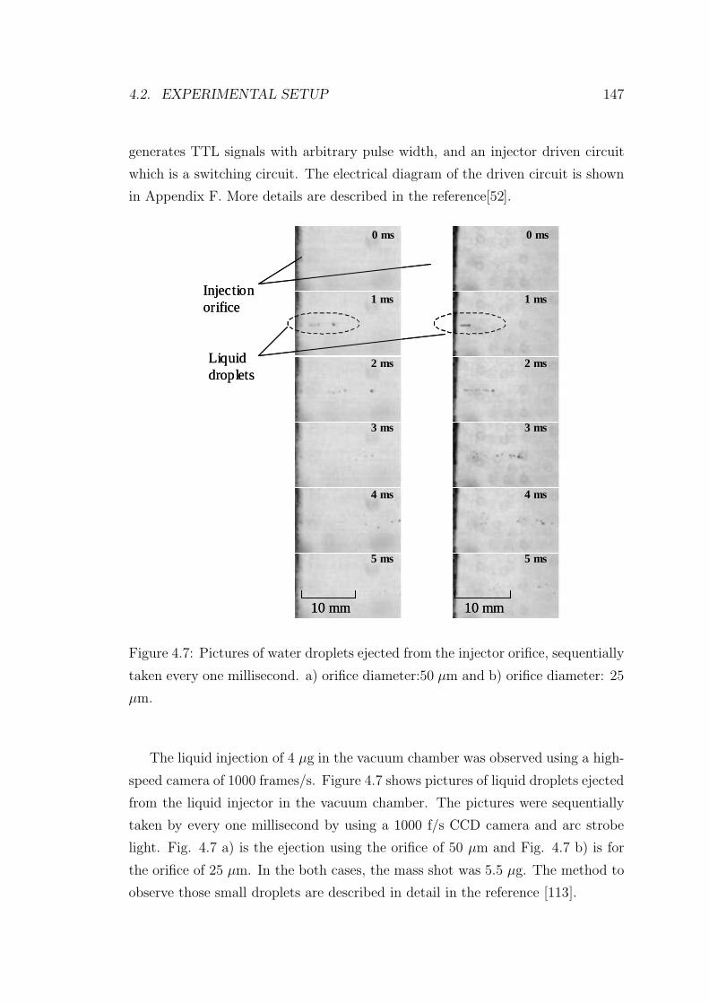
4.2. EXPERIMENTAL SETUP 147
generates TTL signals with arbitrary pulse width, and an injector driven circuit
which is a switching circuit. The electrical diagram of the driven circuit is shown
in Appendix F. More details are described in the reference[52].
10 mm
Injection orifice
10 mm
Liquid droplets
0 ms
1 ms
2 ms
3 ms
4 ms
5 ms
0 ms
1 ms
2 ms
3 ms
4 ms
5 ms
10 mm10 mm
Injection orifice
10 mm10 mm
Liquid droplets
0 ms
1 ms
2 ms
3 ms
4 ms
5 ms
0 ms
1 ms
2 ms
3 ms
4 ms
5 ms
Figure 4.7: Pictures of water droplets ejected from the injector orifice, sequentially
taken every one millisecond. a) orifice diameter:50 µm and b) orifice diameter: 25
µm.
The liquid injection of 4 µg in the vacuum chamber was observed using a high-
speed camera of 1000 frames/s. Figure 4.7 shows pictures of liquid droplets ejected
from the liquid injector in the vacuum chamber. The pictures were sequentially
taken by every one millisecond by using a 1000 f/s CCD camera and arc strobe
light. Fig. 4.7 a) is the ejection using the orifice of 50 µm and Fig. 4.7 b) is for
the orifice of 25 µm. In the both cases, the mass shot was 5.5 µg. The method to
observe those small droplets are described in detail in the reference [113].
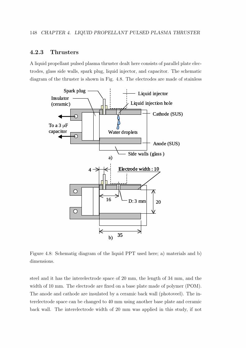
148 CHAPTER 4. LIQUID PROPELLANT PULSED PLASMA THRUSTER
4.2.3 Thrusters
A liquid propellant pulsed plasma thruster dealt here consists of parallel plate elec-
trodes, glass side walls, spark plug, liquid injector, and capacitor. The schematic
diagram of the thruster is shown in Fig. 4.8. The electrodes are made of stainless
Insulator (ceramic)
Anode (SUS)
Cathode (SUS)
Water droplets
Liquid injection hole
Spark plug
Side walls (glass )
To a 3 µFcapacitor
Liquid injector
35
20
Electrode width : 10
16
4
D: 3 mm
a)
b)
Insulator (ceramic)
Anode (SUS)
Cathode (SUS)
Water droplets
Liquid injection hole
Spark plug
Side walls (glass )
To a 3 µFcapacitor
Liquid injector
35
20
Electrode width : 10
16
4
D: 3 mm
35
20
Electrode width : 10
16
4
D: 3 mm
35
20
Electrode width : 10
16
4
D: 3 mm
a)
b)
Figure 4.8: Schematig diagram of the liquid PPT used here; a) materials and b)
dimensions.
steel and it has the interelectrode space of 20 mm, the length of 34 mm, and the
width of 10 mm. The electrode are fixed on a base plate made of polymer (POM).
The anode and cathode are insulated by a ceramic back wall (photoveel). The in-
terelectrode space can be changed to 40 mm using another base plate and ceramic
back wall. The interelectrode width of 20 mm was applied in this study, if not
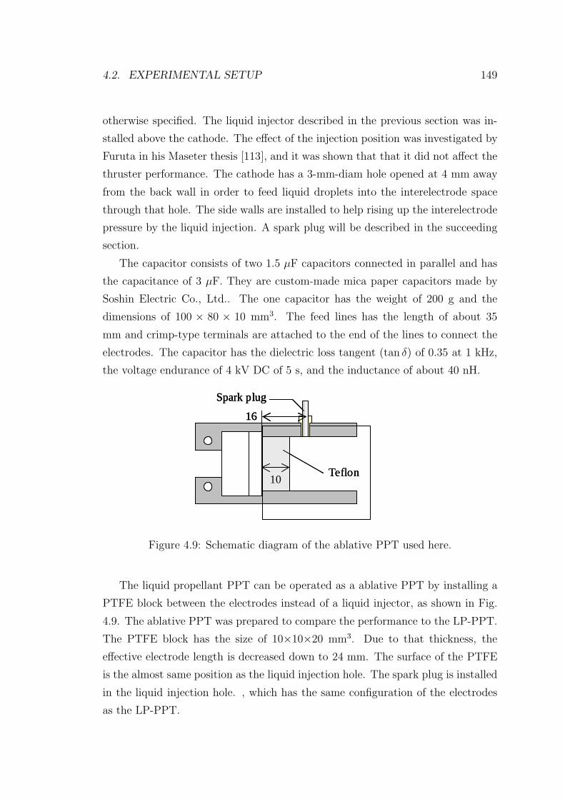
4.2. EXPERIMENTAL SETUP 149
otherwise specified. The liquid injector described in the previous section was in-
stalled above the cathode. The effect of the injection position was investigated by
Furuta in his Maseter thesis [113], and it was shown that that it did not affect the
thruster performance. The cathode has a 3-mm-diam hole opened at 4 mm away
from the back wall in order to feed liquid droplets into the interelectrode space
through that hole. The side walls are installed to help rising up the interelectrode
pressure by the liquid injection. A spark plug will be described in the succeeding
section.
The capacitor consists of two 1.5 µF capacitors connected in parallel and has
the capacitance of 3 µF. They are custom-made mica paper capacitors made by
Soshin Electric Co., Ltd.. The one capacitor has the weight of 200 g and the
dimensions of 100 × 80 × 10 mm3. The feed lines has the length of about 35
mm and crimp-type terminals are attached to the end of the lines to connect the
electrodes. The capacitor has the dielectric loss tangent (tan δ) of 0.35 at 1 kHz,
the voltage endurance of 4 kV DC of 5 s, and the inductance of about 40 nH.
Teflon10
16
Spark plug
Teflon10
16
Spark plug
Teflon10
16
Spark plug
Figure 4.9: Schematic diagram of the ablative PPT used here.
The liquid propellant PPT can be operated as a ablative PPT by installing a
PTFE block between the electrodes instead of a liquid injector, as shown in Fig.
4.9. The ablative PPT was prepared to compare the performance to the LP-PPT.
The PTFE block has the size of 10×10×20 mm3. Due to that thickness, the
effective electrode length is decreased down to 24 mm. The surface of the PTFE
is the almost same position as the liquid injection hole. The spark plug is installed
in the liquid injection hole. , which has the same configuration of the electrodes
as the LP-PPT.
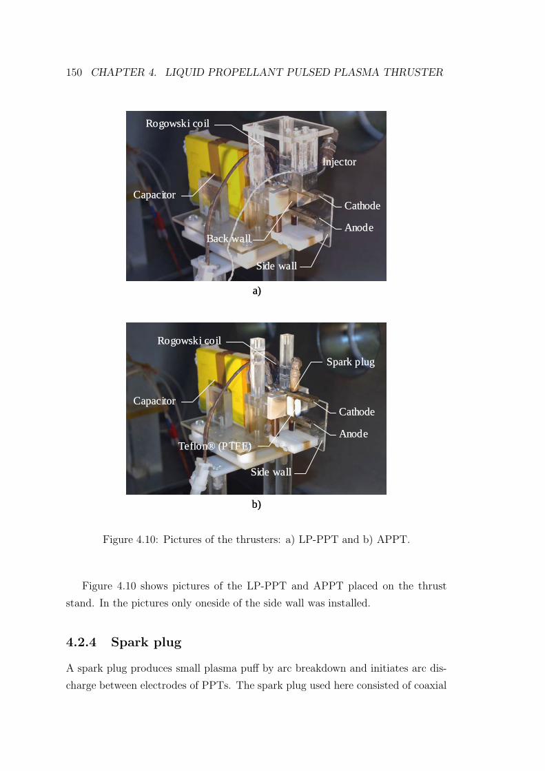
150 CHAPTER 4. LIQUID PROPELLANT PULSED PLASMA THRUSTER
a)
b)
CapacitorCapacitor
InjectorInjector
Side wallSide wall
Back wallBack wall
Spark plugSpark plug
TeflonTeflon®® (PTFE)(PTFE)
Rogowski coilRogowski coil
CathodeCathode
AnodeAnode
CapacitorCapacitor
Side wallSide wall
Rogowski coilRogowski coil
CathodeCathode
AnodeAnode
a)
b)
CapacitorCapacitor
InjectorInjector
Side wallSide wall
Back wallBack wall
Spark plugSpark plug
TeflonTeflon®® (PTFE)(PTFE)
Rogowski coilRogowski coil
CathodeCathode
AnodeAnode
CapacitorCapacitor
Side wallSide wall
Rogowski coilRogowski coil
CathodeCathode
AnodeAnode
Figure 4.10: Pictures of the thrusters: a) LP-PPT and b) APPT.
Figure 4.10 shows pictures of the LP-PPT and APPT placed on the thrust
stand. In the pictures only oneside of the side wall was installed.
4.2.4 Spark plug
A spark plug produces small plasma puff by arc breakdown and initiates arc dis-
charge between electrodes of PPTs. The spark plug used here consisted of coaxial
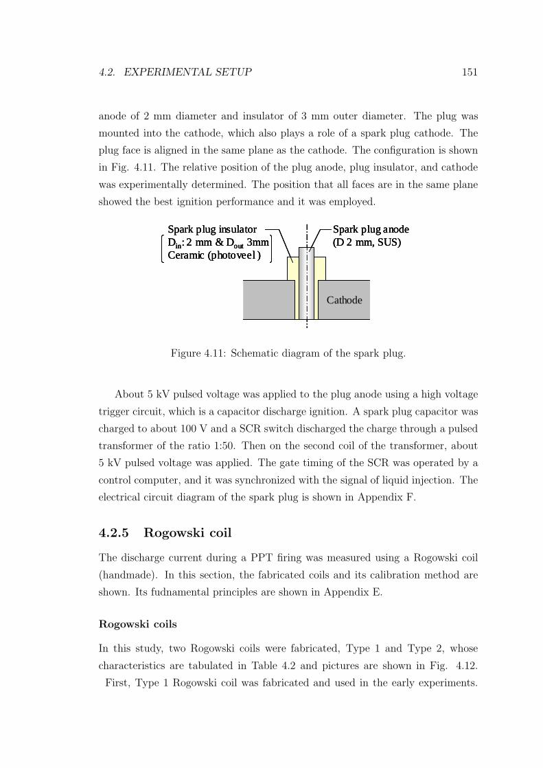
4.2. EXPERIMENTAL SETUP 151
anode of 2 mm diameter and insulator of 3 mm outer diameter. The plug was
mounted into the cathode, which also plays a role of a spark plug cathode. The
plug face is aligned in the same plane as the cathode. The configuration is shown
in Fig. 4.11. The relative position of the plug anode, plug insulator, and cathode
was experimentally determined. The position that all faces are in the same plane
showed the best ignition performance and it was employed.
Spark plug anode(D 2 mm, SUS)
Spark plug insulatorDin: 2 mm & Dout 3mmCeramic (photoveel )
Cathode
Spark plug anode(D 2 mm, SUS)
Spark plug insulatorDin: 2 mm & Dout 3mmCeramic (photoveel )
Cathode
Spark plug anode(D 2 mm, SUS)
Spark plug insulatorDin: 2 mm & Dout 3mmCeramic (photoveel )
Cathode
Figure 4.11: Schematic diagram of the spark plug.
About 5 kV pulsed voltage was applied to the plug anode using a high voltage
trigger circuit, which is a capacitor discharge ignition. A spark plug capacitor was
charged to about 100 V and a SCR switch discharged the charge through a pulsed
transformer of the ratio 1:50. Then on the second coil of the transformer, about
5 kV pulsed voltage was applied. The gate timing of the SCR was operated by a
control computer, and it was synchronized with the signal of liquid injection. The
electrical circuit diagram of the spark plug is shown in Appendix F.
4.2.5 Rogowski coil
The discharge current during a PPT firing was measured using a Rogowski coil
(handmade). In this section, the fabricated coils and its calibration method are
shown. Its fudnamental principles are shown in Appendix E.
Rogowski coils
In this study, two Rogowski coils were fabricated, Type 1 and Type 2, whose
characteristics are tabulated in Table 4.2 and pictures are shown in Fig. 4.12.
First, Type 1 Rogowski coil was fabricated and used in the early experiments.
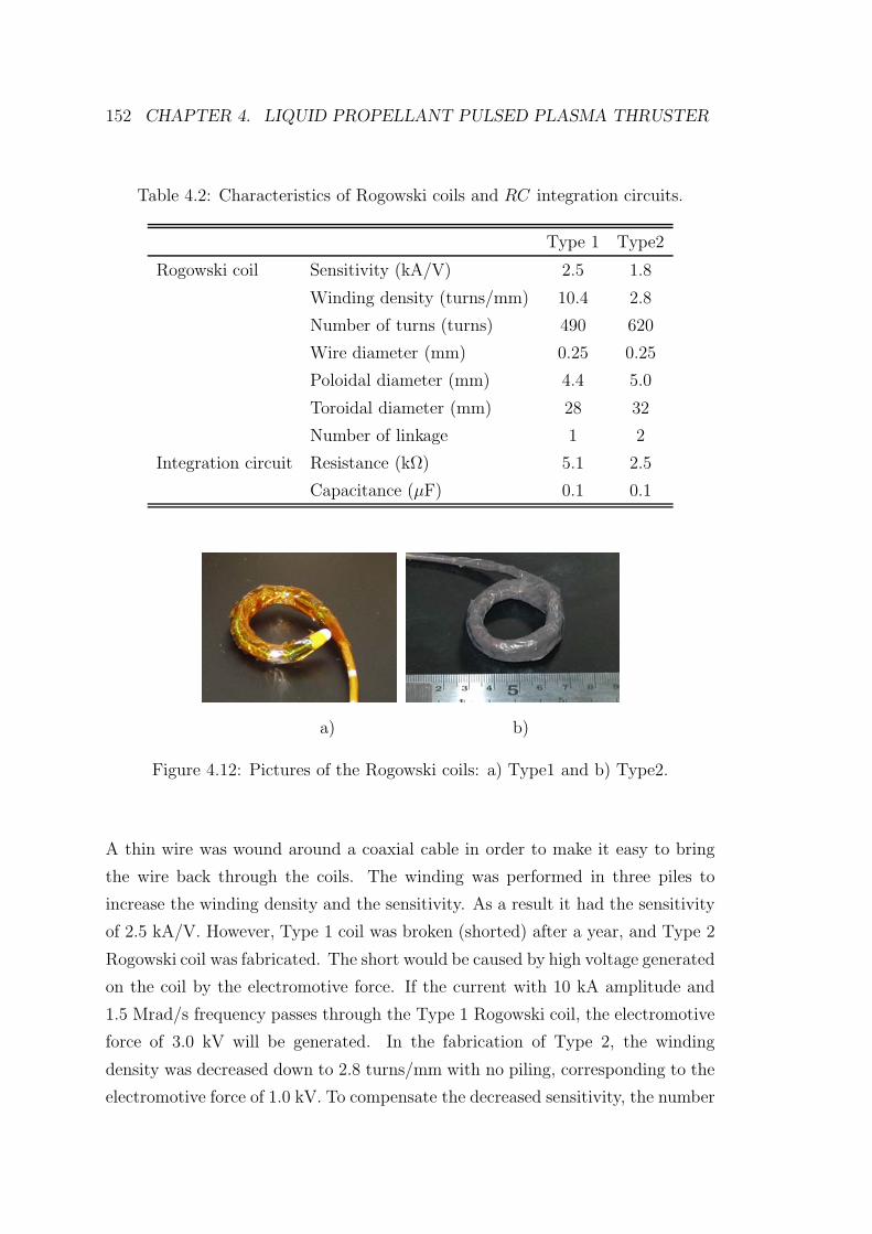
152 CHAPTER 4. LIQUID PROPELLANT PULSED PLASMA THRUSTER
Table 4.2: Characteristics of Rogowski coils and RC integration circuits.
Type 1 Type2
Rogowski coil Sensitivity (kA/V) 2.5 1.8
Winding density (turns/mm) 10.4 2.8
Number of turns (turns) 490 620
Wire diameter (mm) 0.25 0.25
Poloidal diameter (mm) 4.4 5.0
Toroidal diameter (mm) 28 32
Number of linkage 1 2
Integration circuit Resistance (kΩ) 5.1 2.5
Capacitance (µF) 0.1 0.1
a) b)
Figure 4.12: Pictures of the Rogowski coils: a) Type1 and b) Type2.
A thin wire was wound around a coaxial cable in order to make it easy to bring
the wire back through the coils. The winding was performed in three piles to
increase the winding density and the sensitivity. As a result it had the sensitivity
of 2.5 kA/V. However, Type 1 coil was broken (shorted) after a year, and Type 2
Rogowski coil was fabricated. The short would be caused by high voltage generated
on the coil by the electromotive force. If the current with 10 kA amplitude and
1.5 Mrad/s frequency passes through the Type 1 Rogowski coil, the electromotive
force of 3.0 kV will be generated. In the fabrication of Type 2, the winding
density was decreased down to 2.8 turns/mm with no piling, corresponding to the
electromotive force of 1.0 kV. To compensate the decreased sensitivity, the number
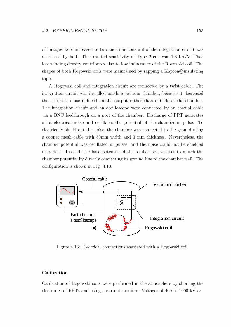
4.2. EXPERIMENTAL SETUP 153
of linkages were increased to two and time constant of the integration circuit was
decreased by half. The resulted sensitivity of Type 2 coil was 1.8 kA/V. That
low winding density contributes also to low inductance of the Rogowski coil. The
shapes of both Rogowski coils were maintained by rapping a Kapton r©insulating
tape.
A Rogowski coil and integration circuit are connected by a twist cable. The
integration circuit was installed inside a vacuum chamber, because it decreased
the electrical noise induced on the output rather than outside of the chamber.
The integration circuit and an oscilloscope were connected by an coaxial cable
via a BNC feedthrough on a port of the chamber. Discharge of PPT generates
a lot electrical noise and oscillates the potential of the chamber in pulse. To
electrically shield out the noise, the chamber was connected to the ground using
a copper mesh cable with 50mm width and 3 mm thickness. Nevertheless, the
chamber potential was oscillated in pulses, and the noise could not be shielded
in perfect. Instead, the base potential of the oscilloscope was set to mutch the
chamber potential by directly connecting its ground line to the chamber wall. The
configuration is shown in Fig. 4.13.
Earth line of a oscilloscope
Rogowski coil
Integration circuit
Coaxial cableVacuum chamber
Earth line of a oscilloscope
Rogowski coil
Integration circuit
Coaxial cableVacuum chamber
Figure 4.13: Electrical connections assoiated with a Rogowski coil.
Calibration
Calibration of Rogowski coils were performed in the atmosphere by shorting the
electrodes of PPTs and using a current monitor. Voltages of 400 to 1000 kV are
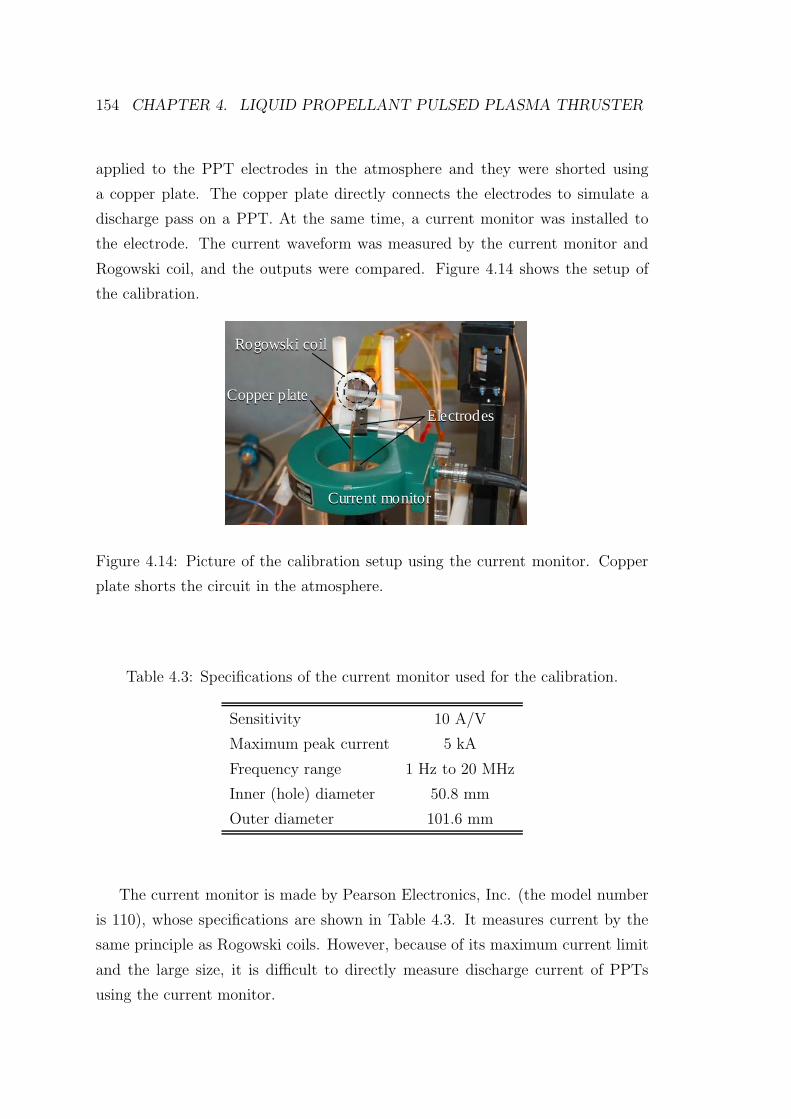
154 CHAPTER 4. LIQUID PROPELLANT PULSED PLASMA THRUSTER
applied to the PPT electrodes in the atmosphere and they were shorted using
a copper plate. The copper plate directly connects the electrodes to simulate a
discharge pass on a PPT. At the same time, a current monitor was installed to
the electrode. The current waveform was measured by the current monitor and
Rogowski coil, and the outputs were compared. Figure 4.14 shows the setup of
the calibration.
Rogowski coil
Current monitor
Copper plateElectrodes
Rogowski coil
Current monitor
Copper plateElectrodes
Rogowski coil
Current monitor
Copper plateElectrodes
Rogowski coil
Current monitor
Copper plateElectrodes
Figure 4.14: Picture of the calibration setup using the current monitor. Copper
plate shorts the circuit in the atmosphere.
Table 4.3: Specifications of the current monitor used for the calibration.
Sensitivity 10 A/V
Maximum peak current 5 kA
Frequency range 1 Hz to 20 MHz
Inner (hole) diameter 50.8 mm
Outer diameter 101.6 mm
The current monitor is made by Pearson Electronics, Inc. (the model number
is 110), whose specifications are shown in Table 4.3. It measures current by the
same principle as Rogowski coils. However, because of its maximum current limit
and the large size, it is difficult to directly measure discharge current of PPTs
using the current monitor.
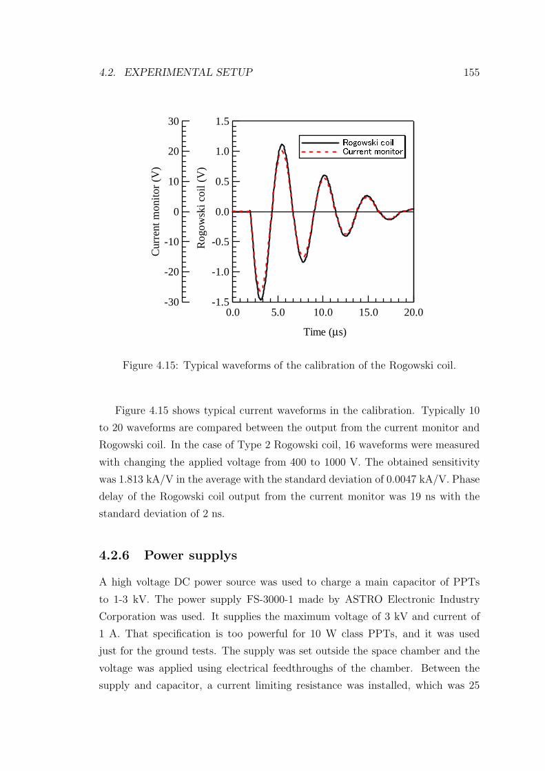
4.2. EXPERIMENTAL SETUP 155
-30
-20
-10
0
10
20
30
Cur
rent
mon
itor
(V
)
20.015.010.05.00.0
Time (µs)
-1.5
-1.0
-0.5
0.0
0.5
1.0
1.5
Rog
owsk
i coi
l (V
)
Rogowski coil Current monitor
Figure 4.15: Typical waveforms of the calibration of the Rogowski coil.
Figure 4.15 shows typical current waveforms in the calibration. Typically 10
to 20 waveforms are compared between the output from the current monitor and
Rogowski coil. In the case of Type 2 Rogowski coil, 16 waveforms were measured
with changing the applied voltage from 400 to 1000 V. The obtained sensitivity
was 1.813 kA/V in the average with the standard deviation of 0.0047 kA/V. Phase
delay of the Rogowski coil output from the current monitor was 19 ns with the
standard deviation of 2 ns.
4.2.6 Power supplys
A high voltage DC power source was used to charge a main capacitor of PPTs
to 1-3 kV. The power supply FS-3000-1 made by ASTRO Electronic Industry
Corporation was used. It supplies the maximum voltage of 3 kV and current of
1 A. That specification is too powerful for 10 W class PPTs, and it was used
just for the ground tests. The supply was set outside the space chamber and the
voltage was applied using electrical feedthroughs of the chamber. Between the
supply and capacitor, a current limiting resistance was installed, which was 25
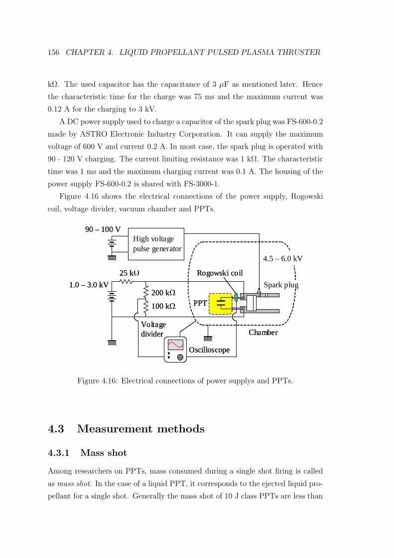
156 CHAPTER 4. LIQUID PROPELLANT PULSED PLASMA THRUSTER
kΩ. The used capacitor has the capacitance of 3 µF as mentioned later. Hence
the characteristic time for the charge was 75 ms and the maximum current was
0.12 A for the charging to 3 kV.
A DC power supply used to charge a capacitor of the spark plug was FS-600-0.2
made by ASTRO Electronic Industry Corporation. It can supply the maximum
voltage of 600 V and current 0.2 A. In most case, the spark plug is operated with
90 - 120 V charging. The current limiting resistance was 1 kΩ. The characteristic
time was 1 ms and the maximum charging current was 0.1 A. The housing of the
power supply FS-600-0.2 is shared with FS-3000-1.
Figure 4.16 shows the electrical connections of the power supply, Rogowski
coil, voltage divider, vacuum chamber and PPTs.
High voltage pulse generator
4.5 – 6.0 kV
1.0 – 3.0 kV
90 – 100 V
25 kΩ
200 kΩ
100 kΩ
Oscilloscope
Chamber
PPT
Spark plug
Rogowski coil
Voltage divider
High voltage pulse generator
4.5 – 6.0 kV
1.0 – 3.0 kV
90 – 100 V
25 kΩ
200 kΩ
100 kΩ
Oscilloscope
Chamber
PPT
Spark plug
Rogowski coil
Voltage divider
Figure 4.16: Electrical connections of power supplys and PPTs.
4.3 Measurement methods
4.3.1 Mass shot
Among researchers on PPTs, mass consumed during a single shot firing is called
as mass shot. In the case of a liquid PPT, it corresponds to the ejected liquid pro-
pellant for a single shot. Generally the mass shot of 10 J class PPTs are less than
4.3. MEASUREMENT METHODS 157
10 µg, and difficult to directly measure such small mass. In most investigations of
ablative PPTs, it is evaluated by the weight difference of a solid propellant before
and after a few thousands of shots.
In this study, the mass shot ∆m was estimated from the pressure increase
in the vacuum chamber ∆P , as well as the laser ablated mass measurement in
Section 3.2.7. The pressure increase is related as ∆m = C∆P , where C is the
proportionality constant. The proportionally constant C was determined dividing
the averaged mass shot by the averaged pressure increase during the experiment.
The averaged mass shot was determined by the weight difference before and after
the experiment. Pressure waveforms in the chamber were all recorded during
the experiment, and the averaged pressure increase was determined. Once the
coefficient was obtained, every mass shot was estimated from the pressure increase.
To obtain the coefficient C , over 2000 shots operation was carried out, which
led to about 20 mg weight difference (mass shot was about 5 - 15 µg). That weight
difference was measured using a precise balance: AB304S by Mettler tredo Co.,
Ltd.. It has the minimum resolution of 0.1 mg and the maximum weight of 320
g. However, attachment of several volatile materials caused the much variations
of the weight measurement. The actual accuracy of the weight measurement here
would be about ±1.0 mg, because the indicator of the balance fluctuated within
±1.0 mg Especially moisture attachment on the injector led to increase of the
weight over 100 mg. To avoid the influence from the total mass shot measurement
of 20 mg, before the experiment the fueled injector was placed in vacuum during
over 2 hours. It vaporized the moisture attached on and stored in the materials of
the injector. After that, the weight of injector was measured as quickly as possible,
and installed again in the vacuum chamber for the experiment. In addition, when
we handled the injector for the weight measurement, we got on latex gloves to
avoid moisture attachment to the injector from our hands.
In contrast, it was difficult to measure the mass shot of an ablative PPT. The
plume ejected from an ablative PPTs contains carbon and fluorine which attaches
on or reacts with a chamber wall. Hence the pressure increase in the chamber is
strongly depends on the configurations of the objects inside the chamber. In short,
the coefficient C can be changed by experiment to experiment. Therefore, instead
of using a pressure, the mass shot was estimated from the energy. It had been
confirmed that the mass shot of ablative PPTs is proportional to the capacitor
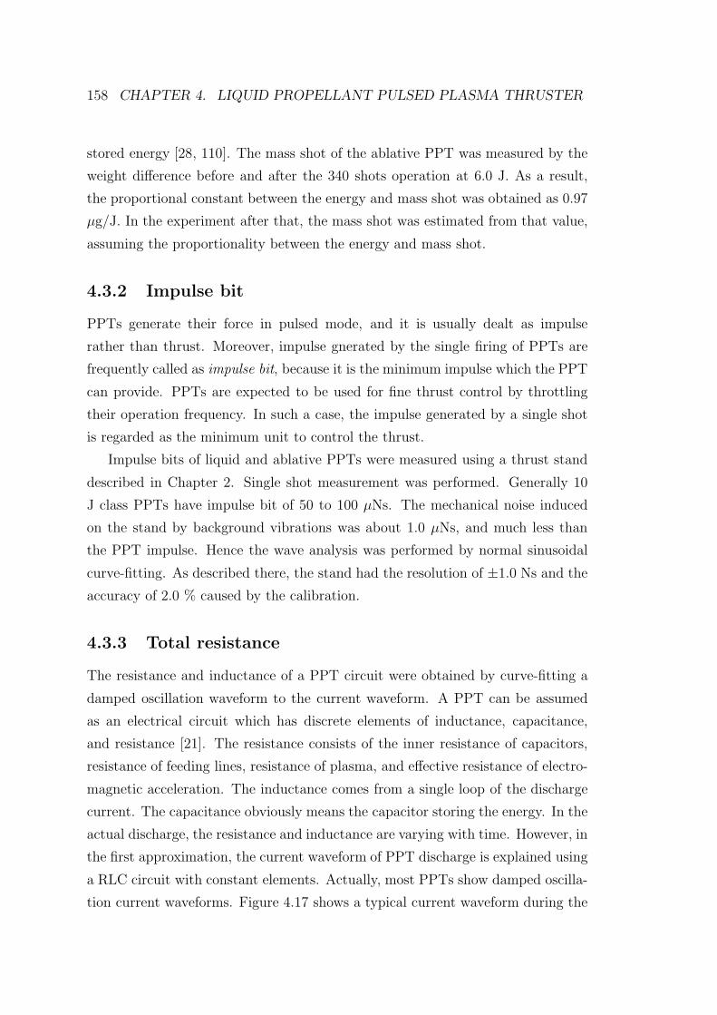
158 CHAPTER 4. LIQUID PROPELLANT PULSED PLASMA THRUSTER
stored energy [28, 110]. The mass shot of the ablative PPT was measured by the
weight difference before and after the 340 shots operation at 6.0 J. As a result,
the proportional constant between the energy and mass shot was obtained as 0.97
µg/J. In the experiment after that, the mass shot was estimated from that value,
assuming the proportionality between the energy and mass shot.
4.3.2 Impulse bit
PPTs generate their force in pulsed mode, and it is usually dealt as impulse
rather than thrust. Moreover, impulse gnerated by the single firing of PPTs are
frequently called as impulse bit, because it is the minimum impulse which the PPT
can provide. PPTs are expected to be used for fine thrust control by throttling
their operation frequency. In such a case, the impulse generated by a single shot
is regarded as the minimum unit to control the thrust.
Impulse bits of liquid and ablative PPTs were measured using a thrust stand
described in Chapter 2. Single shot measurement was performed. Generally 10
J class PPTs have impulse bit of 50 to 100 µNs. The mechanical noise induced
on the stand by background vibrations was about 1.0 µNs, and much less than
the PPT impulse. Hence the wave analysis was performed by normal sinusoidal
curve-fitting. As described there, the stand had the resolution of ±1.0 Ns and the
accuracy of 2.0 % caused by the calibration.
4.3.3 Total resistance
The resistance and inductance of a PPT circuit were obtained by curve-fitting a
damped oscillation waveform to the current waveform. A PPT can be assumed
as an electrical circuit which has discrete elements of inductance, capacitance,
and resistance [21]. The resistance consists of the inner resistance of capacitors,
resistance of feeding lines, resistance of plasma, and effective resistance of electro-
magnetic acceleration. The inductance comes from a single loop of the discharge
current. The capacitance obviously means the capacitor storing the energy. In the
actual discharge, the resistance and inductance are varying with time. However, in
the first approximation, the current waveform of PPT discharge is explained using
a RLC circuit with constant elements. Actually, most PPTs show damped oscilla-
tion current waveforms. Figure 4.17 shows a typical current waveform during the
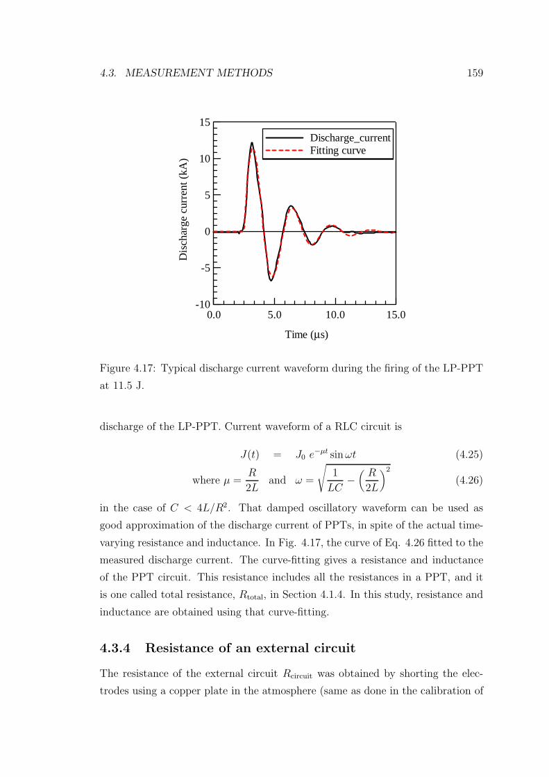
4.3. MEASUREMENT METHODS 159
15
10
5
0
-5
-10
Dis
char
ge c
urre
nt (
kA)
15.010.05.00.0
Time (µs)
Discharge_current Fitting curve
Figure 4.17: Typical discharge current waveform during the firing of the LP-PPT
at 11.5 J.
discharge of the LP-PPT. Current waveform of a RLC circuit is
J(t) = J0 e−µt sinωt (4.25)
where µ =R
2Land ω =
√1
LC−(
R
2L
)2
(4.26)
in the case of C < 4L/R2. That damped oscillatory waveform can be used as
good approximation of the discharge current of PPTs, in spite of the actual time-
varying resistance and inductance. In Fig. 4.17, the curve of Eq. 4.26 fitted to the
measured discharge current. The curve-fitting gives a resistance and inductance
of the PPT circuit. This resistance includes all the resistances in a PPT, and it
is one called total resistance, Rtotal, in Section 4.1.4. In this study, resistance and
inductance are obtained using that curve-fitting.
4.3.4 Resistance of an external circuit
The resistance of the external circuit Rcircuit was obtained by shorting the elec-
trodes using a copper plate in the atmosphere (same as done in the calibration of
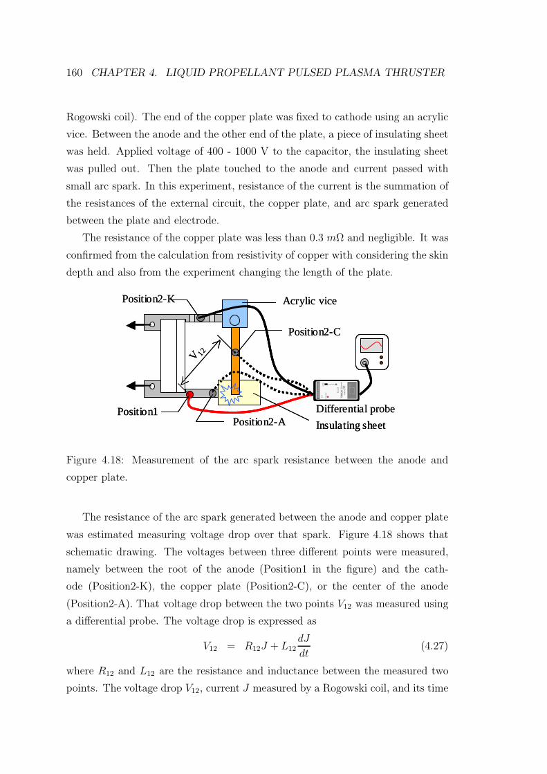
160 CHAPTER 4. LIQUID PROPELLANT PULSED PLASMA THRUSTER
Rogowski coil). The end of the copper plate was fixed to cathode using an acrylic
vice. Between the anode and the other end of the plate, a piece of insulating sheet
was held. Applied voltage of 400 - 1000 V to the capacitor, the insulating sheet
was pulled out. Then the plate touched to the anode and current passed with
small arc spark. In this experiment, resistance of the current is the summation of
the resistances of the external circuit, the copper plate, and arc spark generated
between the plate and electrode.
The resistance of the copper plate was less than 0.3 mΩ and negligible. It was
confirmed from the calculation from resistivity of copper with considering the skin
depth and also from the experiment changing the length of the plate.
Differential probe
Acrylic vice
7009
24D
iffer
entia
lPr
obe
YO
KO
GA
WA
OU
TPU
T M
ax in
to 5
0 k
OV
ER
RA
NG
E
PO
WER
7009
24D
iffer
entia
lPr
obe
YO
KO
GA
WA
OU
TPU
T M
ax in
to 5
0 k
OV
ER
RA
NG
E
PO
WER
Position2-K
Position2-C
Position2-A Insulating sheetPosition1
V 12
Differential probe
Acrylic vice
7009
24D
iffer
entia
lPr
obe
YO
KO
GA
WA
OU
TPU
T M
ax in
to 5
0 k
OV
ER
RA
NG
E
PO
WER
7009
24D
iffer
entia
lPr
obe
YO
KO
GA
WA
OU
TPU
T M
ax in
to 5
0 k
OV
ER
RA
NG
E
PO
WER
7009
24D
iffer
entia
lPr
obe
YO
KO
GA
WA
OU
TPU
T M
ax in
to 5
0 k
OV
ER
RA
NG
E
PO
WER
7009
24D
iffer
entia
lPr
obe
YO
KO
GA
WA
OU
TPU
T M
ax in
to 5
0 k
OV
ER
RA
NG
E
PO
WER
Position2-K
Position2-C
Position2-A Insulating sheetPosition1
V 12
Figure 4.18: Measurement of the arc spark resistance between the anode and
copper plate.
The resistance of the arc spark generated between the anode and copper plate
was estimated measuring voltage drop over that spark. Figure 4.18 shows that
schematic drawing. The voltages between three different points were measured,
namely between the root of the anode (Position1 in the figure) and the cath-
ode (Position2-K), the copper plate (Position2-C), or the center of the anode
(Position2-A). That voltage drop between the two points V12 was measured using
a differential probe. The voltage drop is expressed as
V12 = R12J + L12dJ
dt(4.27)
where R12 and L12 are the resistance and inductance between the measured two
points. The voltage drop V12, current J measured by a Rogowski coil, and its time
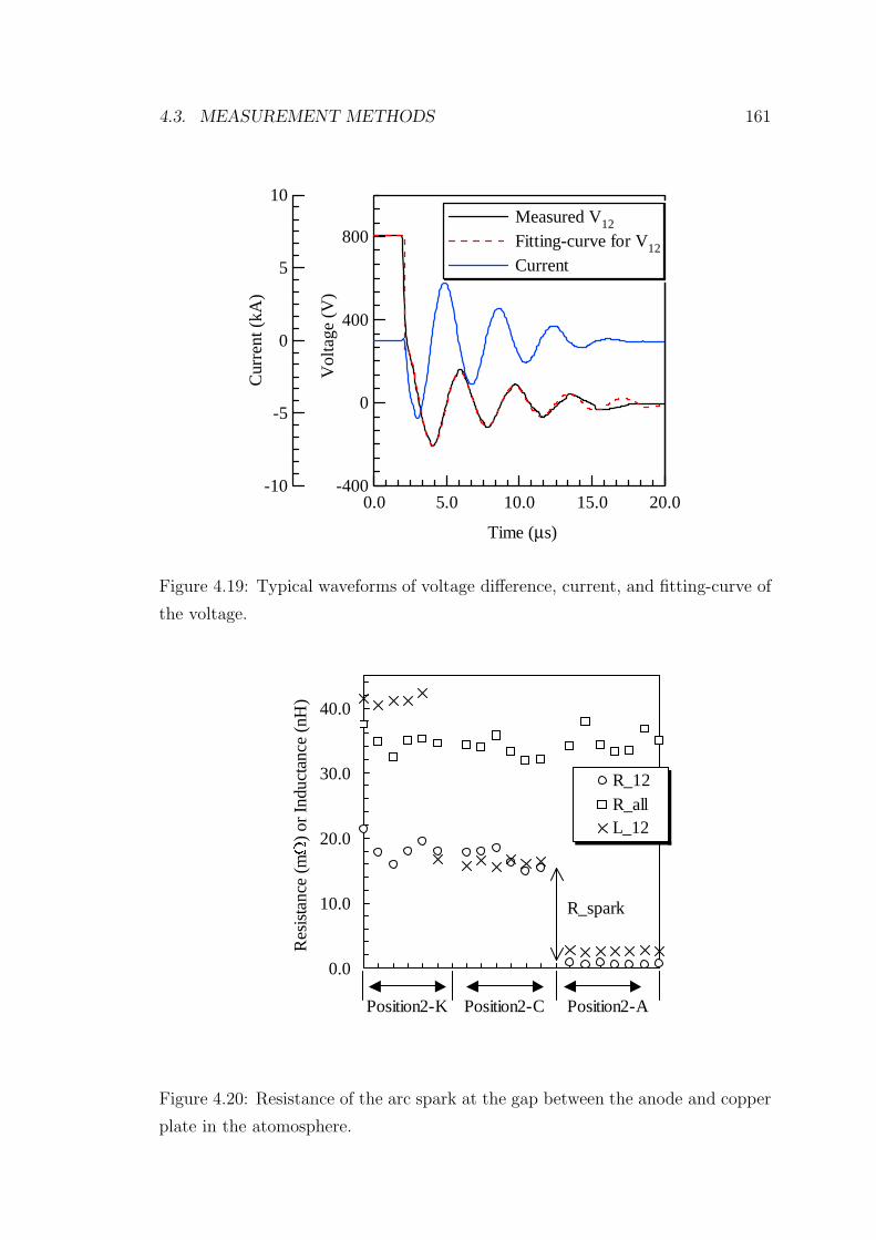
4.3. MEASUREMENT METHODS 161
800
400
0
-400
Vol
tage
(V
)
20.015.010.05.00.0
Time (µs)
-10
-5
0
5
10
Cur
rent
(kA
)
Measured V12
Fitting-curve for V12
Current
Figure 4.19: Typical waveforms of voltage difference, current, and fitting-curve of
the voltage.
0.0
10.0
20.0
30.0
40.0
Res
ista
nce
(m
Ω
) or
Ind
ucta
nce
(nH
)
R_12R_allL_12
Position2-K Position2-C Position2-A
R_spark
Figure 4.20: Resistance of the arc spark at the gap between the anode and copper
plate in the atomosphere.
162 CHAPTER 4. LIQUID PROPELLANT PULSED PLASMA THRUSTER
derivative are fitted to Eq. 4.27 to determin the resistance R12 and inductance
L12. Figure 4.19 shows typical waveforms of measured voltage difference, current,
and fitting-curve of the voltage.
Figure 4.20 is the result of R12 and L12 measurement. The resistances of Posi-
tion 2-K and Position 2-C are almost same, whereas the resistance of Position 2-A
decreases a lot. This difference of the resistance is attributed from he resistance of
arc spark (only Position 2-A did not measure the spark). Therefore, subtracting
this resistance from the total resistance Rall gives the resistance of external circuit
Rcircuit. As a result, the resistance of an external circuit was 17±3 mΩ. The error
comes from the resistance of electrode and the variation of the spark resistance
The variation of the resistance R12 measured at Position 2-K or 2-C is caused by
the arc spark, because the variation of the total resistance Rall matches to it. On
the other hand, inductances are monotonically decreased from 41 to 2.5 nH with
decreases of the measured distance.
4.3.5 Inductance per unit length
The inductance per unit length L′ was measured by changing the position of the
copper plate as shown in Fig 4.21. Different positions of the plate give different in-
ductances. The dependence of the inductance on the position gives the inductance
per unit length. The result is shown in Fig. 4.22 for the case of interelectrode
space of 20 and 40 mm. The inductance is linearly increased by shifting the posi-
tion of the copper plate outward. The inclinations are inductance per unit length
L’, and they are 0.71 and 1.01 nH/mm for 20 and 40 mm electrode respectively.
Figure 4.21: Changing the position of the copper plate to measure the inductance
per unit length.
4.3. MEASUREMENT METHODS 163
Analytical expression for the inductance of a closed circuit of rectangular con-
ductors is [28, 114]
L = 0.4
3
2l + l ln
d
b + c− d + 0.22(b + c)
(4.28)
L (µH), and l, d, b, c (m)
where l and d are the length and height of the closed circuit and b× c is the cross
section of the rectangular conductor in meter. Hence, differentiating the equation
with respect to l,
L′ = 0.6 + 0.4 lnd
b + c(µH), (4.29)
which does not depend on the length l. The electrode used here, of the cross section
of 10×5 mm and the distance of 20 or 40 mm, give L’ of 0.72 and 0.99 nH/mm
respectively. After all, the analytically estimated L’ shows good agreement with
the measured L’, whereas the PPT used here has a rectangular cross section only
with the electrode and the other parts have quite different sections.
120
110
100
90
80
70
Indu
ctan
ce (
nH)
30.020.010.00.0
Distance (mm)
d: 20 mm, L' = 0.71 nH/mm
d: 40 mm, L' = 1.01 nH/mm
Figure 4.22: Dependence of the inductance on the shorting position.
164 CHAPTER 4. LIQUID PROPELLANT PULSED PLASMA THRUSTER
4.4 Experimental Results
Here fundamental characteristics of a liquid PPT were investigated using the
thruster shown in Fig. 4.8. Whereas the thruster had not been optimized, the
characteristics of a liquid PPT was clarified by comparing it to an ablative PPT.
The used ablative thruster is shown in Fig. 4.9.
4.4.1 Mass shot vs. Impulse bit
The impulse bit of a liquid PPT was shown not to depend on the mass shot,
namely injected propellant by liquid injector for a single shot. Essentially the
electromagnetic impulse of PPTs does not depend on the mass shot, as indicated
by Eq. 4.24. On the other hand, electrothermal acceleration will be proportional
to the square root of the mass shot. It means that the impulse by a liquid PPT
was produced mainly by electromagnetic acceleration.
Figure 4.23 shows the dependence of impulse bit on the mass shot operated
at the energy of 10.0 J (2.6 kV). The error bars in the figure show the standard
deviations of five shots. The impulse is slightly increased with the increase of the
mass shot. The slope of the regression line is 467 m/s. It corresponds to the
expected cold gas velocity. Therefore the slight increase of the impulse would be
caused by the increase of the cold gas thrust, not electrothermal acceleration.
Constant impulse bit on the mass shot means that the specific impulse is
inversely proportional to it. Figure 4.24 show the specific impulse calculatd from
the impulse bit and mass shot. At the mass shot of 3.0 µg, it reaches over 2000
s. At the higher energy operation, it reached to 3000 s (such high Isp operation
was investigated by Kakami [52]). It should be noted here that small mass shot
operation also causes a lot of varieties of impulse bits. It would be because that
too small mass shot makes it difficult to initiate discharge.
4.4.2 Energy vs. Impulse bit
The impulse bit of a liquid PPT was linearly increased with the increase of the
capacitor stored energy. It is expected from the theory of electromagnetic impulse
Eq. 4.24. Figure 4.25 shows the impulse bit dependence of the energy. There
the impulse bit using another electrode distance of 40 mm is also shown. The
4.4. EXPERIMENTAL RESULTS 165
80.0
60.0
40.0
20.0
0.0
Impu
lse
bit (
µNs)
20.015.010.05.00.0
Mass shot (µg)
I = 0.467 M + 56.5
Figure 4.23: Impulse bit dependence on the mass shot in the LP-PPT at 10.0 J
(2.6 kV).
2500
2000
1500
1000
500
0
Spe
cifi
c Im
puls
e (s
)
20.015.010.05.00.0
Mass shot (µg)
Figure 4.24: Specific impulse dependence on the mass shot in the LP-PPT at 10.0
J (2.6 kV).
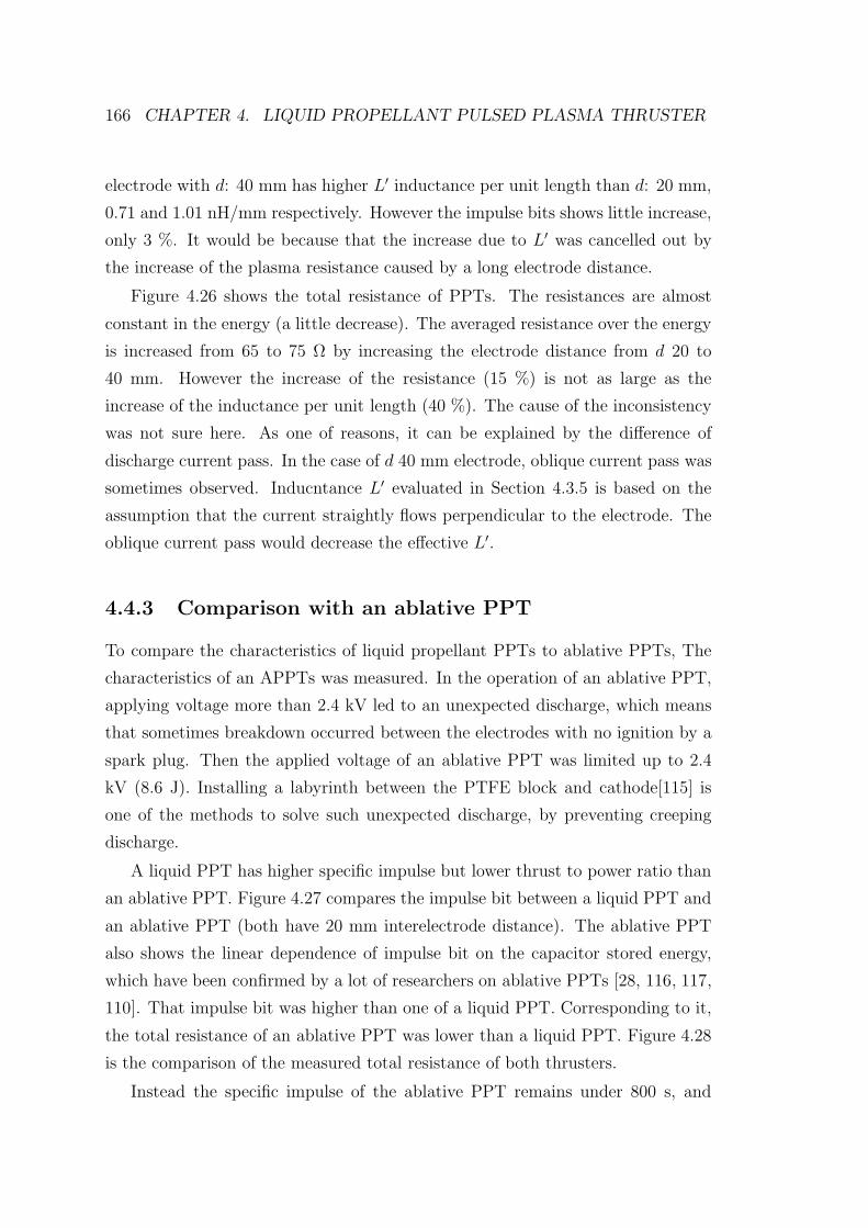
166 CHAPTER 4. LIQUID PROPELLANT PULSED PLASMA THRUSTER
electrode with d: 40 mm has higher L′ inductance per unit length than d: 20 mm,
0.71 and 1.01 nH/mm respectively. However the impulse bits shows little increase,
only 3 %. It would be because that the increase due to L′ was cancelled out by
the increase of the plasma resistance caused by a long electrode distance.
Figure 4.26 shows the total resistance of PPTs. The resistances are almost
constant in the energy (a little decrease). The averaged resistance over the energy
is increased from 65 to 75 Ω by increasing the electrode distance from d 20 to
40 mm. However the increase of the resistance (15 %) is not as large as the
increase of the inductance per unit length (40 %). The cause of the inconsistency
was not sure here. As one of reasons, it can be explained by the difference of
discharge current pass. In the case of d 40 mm electrode, oblique current pass was
sometimes observed. Inducntance L′ evaluated in Section 4.3.5 is based on the
assumption that the current straightly flows perpendicular to the electrode. The
oblique current pass would decrease the effective L′.
4.4.3 Comparison with an ablative PPT
To compare the characteristics of liquid propellant PPTs to ablative PPTs, The
characteristics of an APPTs was measured. In the operation of an ablative PPT,
applying voltage more than 2.4 kV led to an unexpected discharge, which means
that sometimes breakdown occurred between the electrodes with no ignition by a
spark plug. Then the applied voltage of an ablative PPT was limited up to 2.4
kV (8.6 J). Installing a labyrinth between the PTFE block and cathode[115] is
one of the methods to solve such unexpected discharge, by preventing creeping
discharge.
A liquid PPT has higher specific impulse but lower thrust to power ratio than
an ablative PPT. Figure 4.27 compares the impulse bit between a liquid PPT and
an ablative PPT (both have 20 mm interelectrode distance). The ablative PPT
also shows the linear dependence of impulse bit on the capacitor stored energy,
which have been confirmed by a lot of researchers on ablative PPTs [28, 116, 117,
110]. That impulse bit was higher than one of a liquid PPT. Corresponding to it,
the total resistance of an ablative PPT was lower than a liquid PPT. Figure 4.28
is the comparison of the measured total resistance of both thrusters.
Instead the specific impulse of the ablative PPT remains under 800 s, and
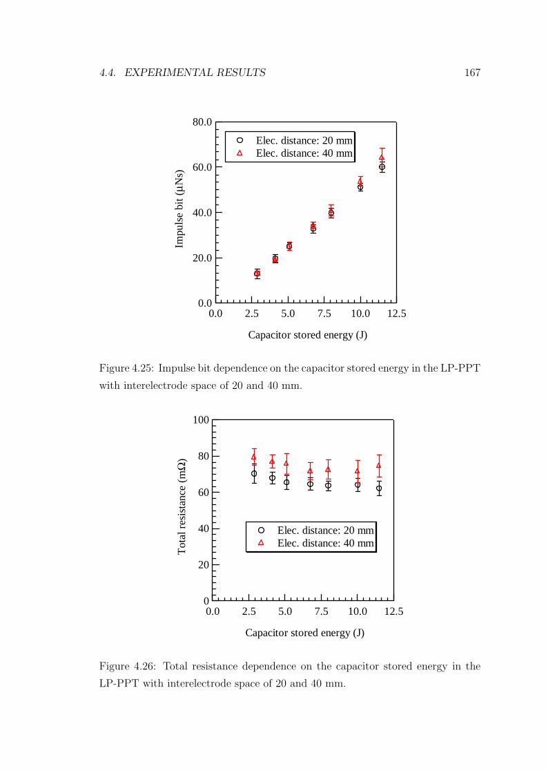
4.4. EXPERIMENTAL RESULTS 167
80.0
60.0
40.0
20.0
0.0
Impu
lse
bit (
µNs)
12.510.07.55.02.50.0
Capacitor stored energy (J)
Elec. distance: 20 mm Elec. distance: 40 mm
Figure 4.25: Impulse bit dependence on the capacitor stored energy in the LP-PPT
with interelectrode space of 20 and 40 mm.
100
80
60
40
20
0
Tot
al r
esis
tanc
e (m
Ω)
12.510.07.55.02.50.0
Capacitor stored energy (J)
Elec. distance: 20 mm Elec. distance: 40 mm
Figure 4.26: Total resistance dependence on the capacitor stored energy in the
LP-PPT with interelectrode space of 20 and 40 mm.
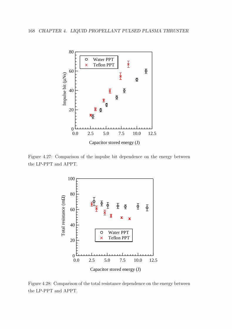
168 CHAPTER 4. LIQUID PROPELLANT PULSED PLASMA THRUSTER
80
60
40
20
0
Impu
lse
bit (
µNs)
12.510.07.55.02.50.0
Capacitor stored energy (J)
Water PPT Teflon PPT
Figure 4.27: Comparison of the impulse bit dependence on the energy between
the LP-PPT and APPT.
100
80
60
40
20
0
Tot
al r
esis
tanc
e (m
Ω)
12.510.07.55.02.50.0
Capacitor stored energy (J)
Water PPT Teflon PPT
Figure 4.28: Comparison of the total resistance dependence on the energy between
the LP-PPT and APPT.
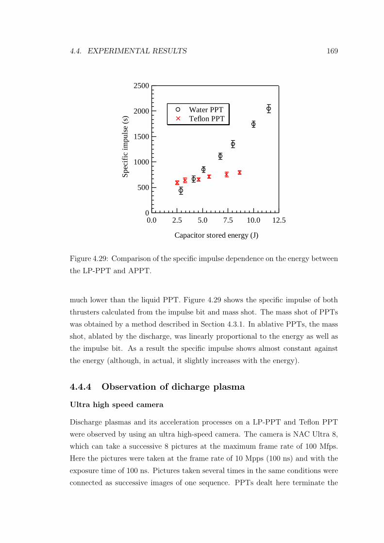
4.4. EXPERIMENTAL RESULTS 169
2500
2000
1500
1000
500
0
Spe
cifi
c im
puls
e (s
)
12.510.07.55.02.50.0
Capacitor stored energy (J)
Water PPT Teflon PPT
Figure 4.29: Comparison of the specific impulse dependence on the energy between
the LP-PPT and APPT.
much lower than the liquid PPT. Figure 4.29 shows the specific impulse of both
thrusters calculated from the impulse bit and mass shot. The mass shot of PPTs
was obtained by a method described in Section 4.3.1. In ablative PPTs, the mass
shot, ablated by the discharge, was linearly proportional to the energy as well as
the impulse bit. As a result the specific impulse shows almost constant against
the energy (although, in actual, it slightly increases with the energy).
4.4.4 Observation of dicharge plasma
Ultra high speed camera
Discharge plasmas and its acceleration processes on a LP-PPT and Teflon PPT
were observed by using an ultra high-speed camera. The camera is NAC Ultra 8,
which can take a successive 8 pictures at the maximum frame rate of 100 Mfps.
Here the pictures were taken at the frame rate of 10 Mpps (100 ns) and with the
exposure time of 100 ns. Pictures taken several times in the same conditions were
connected as successive images of one sequence. PPTs dealt here terminate the
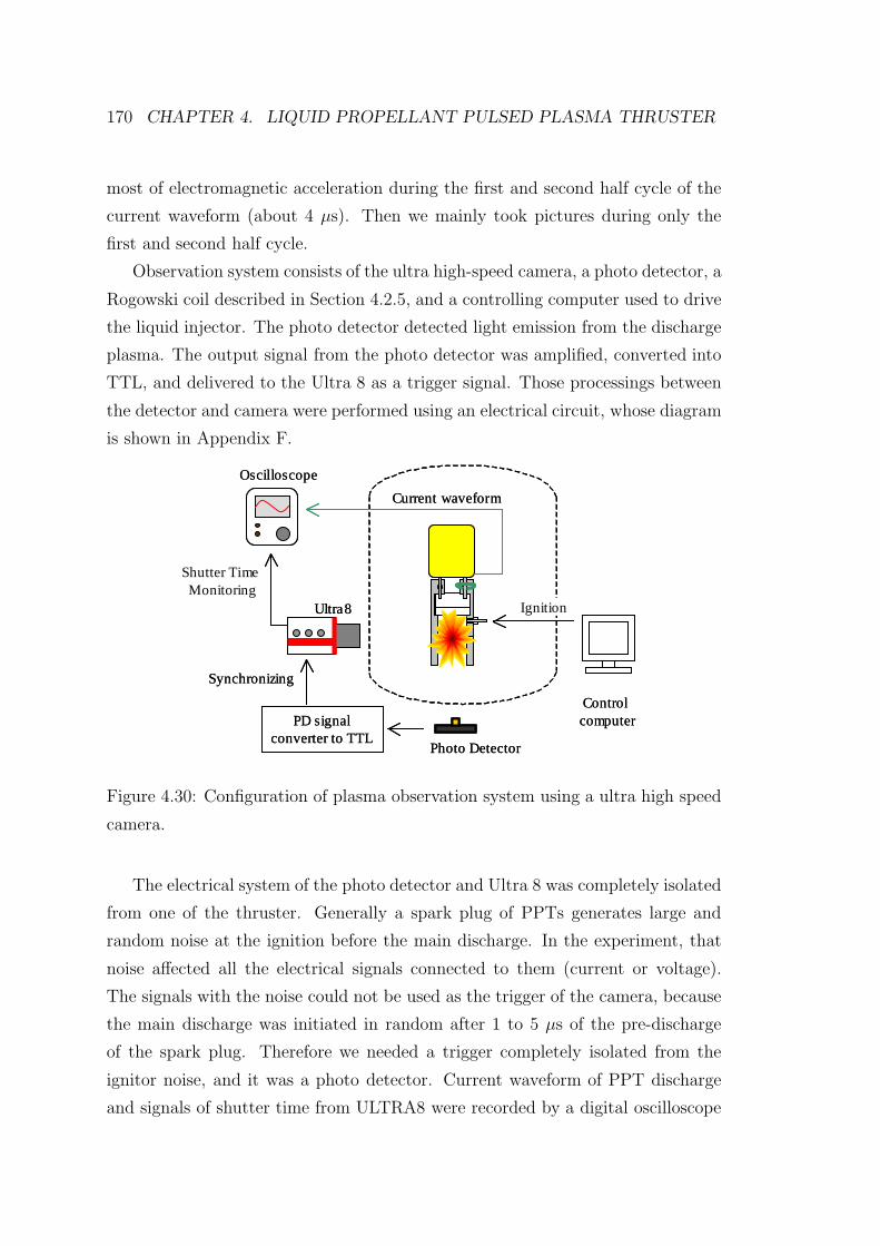
170 CHAPTER 4. LIQUID PROPELLANT PULSED PLASMA THRUSTER
most of electromagnetic acceleration during the first and second half cycle of the
current waveform (about 4 µs). Then we mainly took pictures during only the
first and second half cycle.
Observation system consists of the ultra high-speed camera, a photo detector, a
Rogowski coil described in Section 4.2.5, and a controlling computer used to drive
the liquid injector. The photo detector detected light emission from the discharge
plasma. The output signal from the photo detector was amplified, converted into
TTL, and delivered to the Ultra 8 as a trigger signal. Those processings between
the detector and camera were performed using an electrical circuit, whose diagram
is shown in Appendix F.
Control computer
Photo Detector
Oscilloscope
Ultra8
PD signal converter to TTL
Synchronizing
Shutter Time Monitoring
Current waveform
Ignition
Control computer
Photo Detector
Oscilloscope
Ultra8
PD signal converter to TTL
Synchronizing
Shutter Time Monitoring
Current waveform
Ignition
Figure 4.30: Configuration of plasma observation system using a ultra high speed
camera.
The electrical system of the photo detector and Ultra 8 was completely isolated
from one of the thruster. Generally a spark plug of PPTs generates large and
random noise at the ignition before the main discharge. In the experiment, that
noise affected all the electrical signals connected to them (current or voltage).
The signals with the noise could not be used as the trigger of the camera, because
the main discharge was initiated in random after 1 to 5 µs of the pre-discharge
of the spark plug. Therefore we needed a trigger completely isolated from the
ignitor noise, and it was a photo detector. Current waveform of PPT discharge
and signals of shutter time from ULTRA8 were recorded by a digital oscilloscope
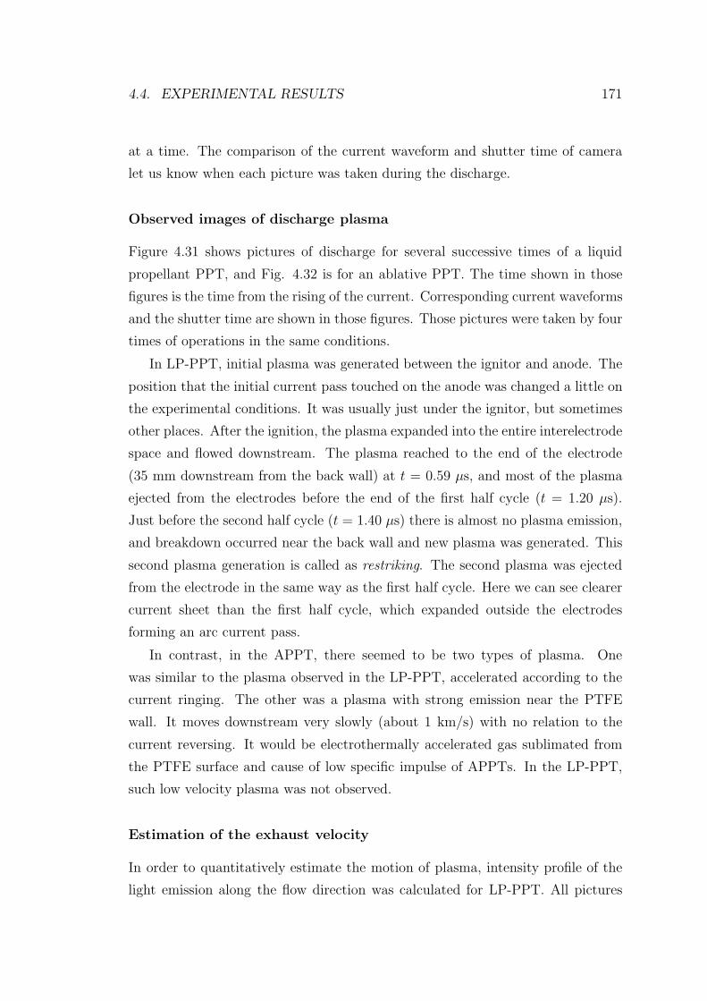
4.4. EXPERIMENTAL RESULTS 171
at a time. The comparison of the current waveform and shutter time of camera
let us know when each picture was taken during the discharge.
Observed images of discharge plasma
Figure 4.31 shows pictures of discharge for several successive times of a liquid
propellant PPT, and Fig. 4.32 is for an ablative PPT. The time shown in those
figures is the time from the rising of the current. Corresponding current waveforms
and the shutter time are shown in those figures. Those pictures were taken by four
times of operations in the same conditions.
In LP-PPT, initial plasma was generated between the ignitor and anode. The
position that the initial current pass touched on the anode was changed a little on
the experimental conditions. It was usually just under the ignitor, but sometimes
other places. After the ignition, the plasma expanded into the entire interelectrode
space and flowed downstream. The plasma reached to the end of the electrode
(35 mm downstream from the back wall) at t = 0.59 µs, and most of the plasma
ejected from the electrodes before the end of the first half cycle (t = 1.20 µs).
Just before the second half cycle (t = 1.40 µs) there is almost no plasma emission,
and breakdown occurred near the back wall and new plasma was generated. This
second plasma generation is called as restriking. The second plasma was ejected
from the electrode in the same way as the first half cycle. Here we can see clearer
current sheet than the first half cycle, which expanded outside the electrodes
forming an arc current pass.
In contrast, in the APPT, there seemed to be two types of plasma. One
was similar to the plasma observed in the LP-PPT, accelerated according to the
current ringing. The other was a plasma with strong emission near the PTFE
wall. It moves downstream very slowly (about 1 km/s) with no relation to the
current reversing. It would be electrothermally accelerated gas sublimated from
the PTFE surface and cause of low specific impulse of APPTs. In the LP-PPT,
such low velocity plasma was not observed.
Estimation of the exhaust velocity
In order to quantitatively estimate the motion of plasma, intensity profile of the
light emission along the flow direction was calculated for LP-PPT. All pictures
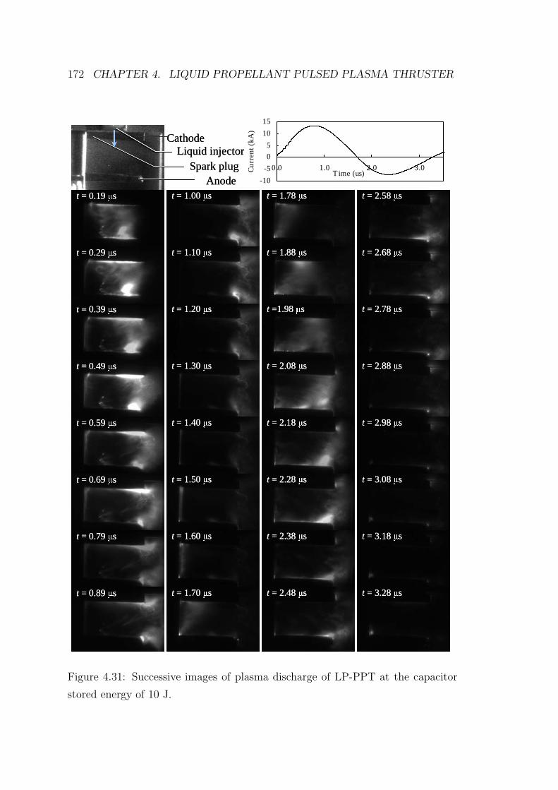
172 CHAPTER 4. LIQUID PROPELLANT PULSED PLASMA THRUSTER
Liquid injectorSpark plug
Cathode
Anodet = 0.19 µs
t = 0.29 µs
t = 0.39 µs
t = 0.49 µs
t = 0.59 µs
t = 0.69 µs
t = 0.79 µs
t = 0.89 µs
t = 1.00 µs
t = 1.10 µs
t = 1.20 µs
t = 1.30 µs
t = 1.40 µs
t = 1.50 µs
t = 1.60 µs
t = 1.70 µs
t = 1.78 µs
t = 1.88 µs
t =1.98 µs
t = 2.08 µs
t = 2.18 µs
t = 2.28 µs
t = 2.38 µs
t = 2.48 µs
t = 2.58 µs
t = 2.68 µs
t = 2.78 µs
t = 2.88 µs
t = 2.98 µs
t = 3.08 µs
t = 3.18 µs
t = 3.28 µs
-10
-5
0
5
10
15
0.0 1.0 2.0 3.0Time (us)C
urre
nt (
kA)
Liquid injectorSpark plug
Cathode
Anodet = 0.19 µs
t = 0.29 µs
t = 0.39 µs
t = 0.49 µs
t = 0.59 µs
t = 0.69 µs
t = 0.79 µs
t = 0.89 µs
t = 0.19 µs
t = 0.29 µs
t = 0.39 µs
t = 0.49 µs
t = 0.59 µs
t = 0.69 µs
t = 0.79 µs
t = 0.89 µs
t = 1.00 µs
t = 1.10 µs
t = 1.20 µs
t = 1.30 µs
t = 1.40 µs
t = 1.50 µs
t = 1.60 µs
t = 1.70 µs
t = 1.00 µs
t = 1.10 µs
t = 1.20 µs
t = 1.30 µs
t = 1.40 µs
t = 1.50 µs
t = 1.60 µs
t = 1.70 µs
t = 1.78 µs
t = 1.88 µs
t =1.98 µs
t = 2.08 µs
t = 2.18 µs
t = 2.28 µs
t = 2.38 µs
t = 2.48 µs
t = 1.78 µs
t = 1.88 µs
t =1.98 µs
t = 2.08 µs
t = 2.18 µs
t = 2.28 µs
t = 2.38 µs
t = 2.48 µs
t = 2.58 µs
t = 2.68 µs
t = 2.78 µs
t = 2.88 µs
t = 2.98 µs
t = 3.08 µs
t = 3.18 µs
t = 3.28 µs
t = 2.58 µs
t = 2.68 µs
t = 2.78 µs
t = 2.88 µs
t = 2.98 µs
t = 3.08 µs
t = 3.18 µs
t = 3.28 µs
-10
-5
0
5
10
15
0.0 1.0 2.0 3.0Time (us)C
urre
nt (
kA)
Figure 4.31: Successive images of plasma discharge of LP-PPT at the capacitor
stored energy of 10 J.
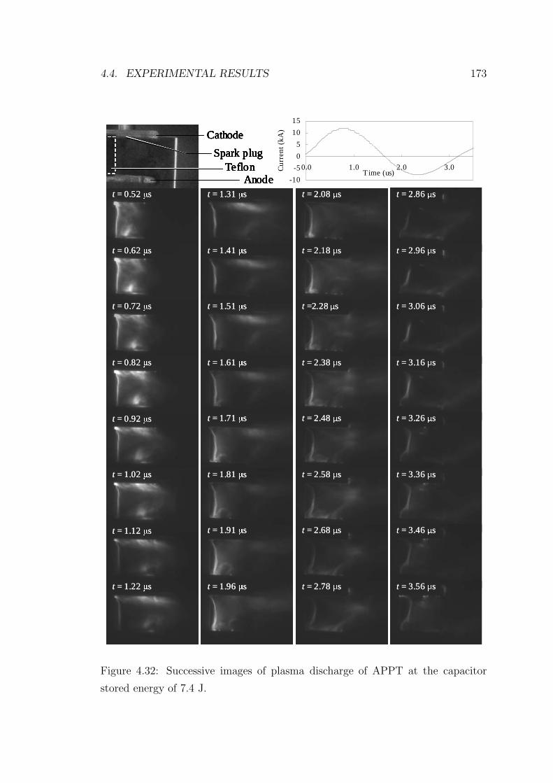
4.4. EXPERIMENTAL RESULTS 173
-10
-5
0
5
10
15
0.0 1.0 2.0 3.0Time (us)C
urre
nt (
kA)
TeflonSpark plug
Cathode
Anodet = 0.52 µs
t = 0.62 µs
t = 0.72 µs
t = 0.82 µs
t = 0.92 µs
t = 1.02 µs
t = 1.12 µs
t = 1.22 µs
t = 1.31 µs
t = 1.41 µs
t = 1.51 µs
t = 1.61 µs
t = 1.71 µs
t = 1.81 µs
t = 1.91 µs
t = 1.96 µs
t = 2.08 µs
t = 2.18 µs
t =2.28 µs
t = 2.38 µs
t = 2.48 µs
t = 2.58 µs
t = 2.68 µs
t = 2.78 µs
t = 2.86 µs
t = 2.96 µs
t = 3.06 µs
t = 3.16 µs
t = 3.26 µs
t = 3.36 µs
t = 3.46 µs
t = 3.56 µs
TeflonSpark plug
Cathode
AnodeTeflon
Spark plug
Cathode
AnodeTeflon
Spark plug
Cathode
AnodeTeflon
Spark plug
Cathode
Anodet = 0.52 µs
t = 0.62 µs
t = 0.72 µs
t = 0.82 µs
t = 0.92 µs
t = 1.02 µs
t = 1.12 µs
t = 1.22 µs
t = 0.52 µs
t = 0.62 µs
t = 0.72 µs
t = 0.82 µs
t = 0.92 µs
t = 1.02 µs
t = 1.12 µs
t = 1.22 µs
t = 1.31 µs
t = 1.41 µs
t = 1.51 µs
t = 1.61 µs
t = 1.71 µs
t = 1.81 µs
t = 1.91 µs
t = 1.96 µs
t = 1.31 µs
t = 1.41 µs
t = 1.51 µs
t = 1.61 µs
t = 1.71 µs
t = 1.81 µs
t = 1.91 µs
t = 1.96 µs
t = 2.08 µs
t = 2.18 µs
t =2.28 µs
t = 2.38 µs
t = 2.48 µs
t = 2.58 µs
t = 2.68 µs
t = 2.78 µs
t = 2.08 µs
t = 2.18 µs
t =2.28 µs
t = 2.38 µs
t = 2.48 µs
t = 2.58 µs
t = 2.68 µs
t = 2.78 µs
t = 2.86 µs
t = 2.96 µs
t = 3.06 µs
t = 3.16 µs
t = 3.26 µs
t = 3.36 µs
t = 3.46 µs
t = 3.56 µs
t = 2.86 µs
t = 2.96 µs
t = 3.06 µs
t = 3.16 µs
t = 3.26 µs
t = 3.36 µs
t = 3.46 µs
t = 3.56 µs
Figure 4.32: Successive images of plasma discharge of APPT at the capacitor
stored energy of 7.4 J.
174 CHAPTER 4. LIQUID PROPELLANT PULSED PLASMA THRUSTER
were converted into numerical data of the light intensity. The data were integrated
in a longitudinal direction (vertical to the electrode), and intensity profiles of the
lateral direction (parallel to the electrode) were obtained. Figure 4.33 shows the
lateral direction intensity profiles at the time from 0.2 to 3.3 µs; Fig. 4.33 a) is
during the first half cycle and b) is during the second half cycle.
Figure 4.34 shows the time history of an averaged position of the light emission,
calculated using the profiles of Fig. 4.33. In the figure, the corresponding squared
current waveform is also shown. Here the averaged position of plasma was defined
as the gravity center of the intensity profile, expressed by
zG.C.(t) ≡∫ L
0zI(z, t) dx
/∫ L
0I(z, t) dx (4.30)
where I(z, t) is the intensity profile shown in Fig. 4.33. First, the average position
goes downstream with the averaged velocity of 33 km/s. After that, the position
remained around 35 mm, whereas the actual plasma is ejected from the electrode.
It is because the most of plasma flew outside the observed area and strong emission
around the edge of the electrodes. In the second half cycle, a new plasma is
generated on the back wall and it proceeds downstream with the averaged velocity
of 43 km/s.
That exhaust velocity is much higher than one estimated from the thrust and
mass shot. It means the actually accelerated plasma is much less than the mass
shot. In other words, only a fraction of the injected liquid was electromagnetically
accelerated as plasma.
It should be cared that the above estimated velocities are not the actual plasma
velocity, because the emission from plasma does not mean the density. If the
electron reaches to the local equilibrium with respect to its excitation temperature,
the emission will be proportional to the density. Moreover, the velocities are
obtained only in the beginning of the every half cycle. Further acceleration outside
the electrode was neglected. Neverthless, let us roughly estimate the equivalent
resistance of electromagnetic acceleration using those velocities. Equation 4.19 is
further simplified as
v =∑n
∫nth1/2cycle
vnJ2 dt
/∫ ∞
0J2 dt (4.31)
(v1
∫ T/2
0J2 dt + v2
∫ T
T/2J2 dt
)/∫ T
0J2 dt (4.32)
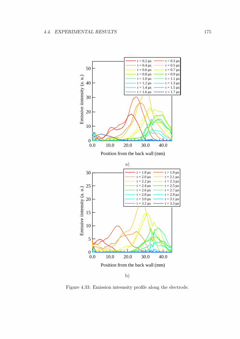
4.4. EXPERIMENTAL RESULTS 175
50
40
30
20
10
0
Em
issi
ve ii
nten
sity
(a.
u.)
40.030.020.010.00.0
Position from the back wall (mm)
t = 0.2 µs t = 0.3 µs t = 0.4 µs t = 0.5 µs t = 0.6 µs t = 0.7 µs t = 0.8 µs t = 0.9 µs t = 1.0 µs t = 1.1 µs t = 1.2 µs t = 1.3 µs t = 1.4 µs t = 1.5 µs t = 1.6 µs t = 1.7 µs
a)
30
25
20
15
10
5
0
Em
issi
ve ii
nten
sity
(a.
u.)
40.030.020.010.00.0
Position from the back wall (mm)
t = 1.8 µs t = 1.9 µs t = 2.0 µs t = 2.1 µs t = 2.2 µs t = 2.3 µs t = 2.4 µs t = 2.5 µs t = 2.6 µs t = 2.7 µs t = 2.8 µs t = 2.9 µs t = 3.0 µs t = 3.1 µs t = 3.2 µs t = 3.3 µs
b)
Figure 4.33: Emission intesnsity profile along the electrode.
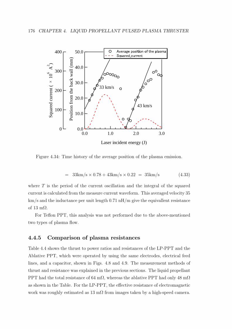
176 CHAPTER 4. LIQUID PROPELLANT PULSED PLASMA THRUSTER
50.0
40.0
30.0
20.0
10.0
0.0
Pos
ition
fro
m th
e ba
ck w
all (
mm
)
3.02.01.00.0
Laser incident energy (J)
400
300
200
100
0
Squ
ared
cur
rent
(10
6 A2 )
33 km/s
43 km/s
Average position of the plasma
Squared_current
Figure 4.34: Time history of the average position of the plasma emission.
= 33km/s × 0.78 + 43km/s × 0.22 = 35km/s (4.33)
where T is the period of the current oscillation and the integral of the squared
current is calculated from the measure current waveform. This averaged velocity 35
km/s and the inductance per unit length 0.71 nH/m give the equivallent resistance
of 13 mΩ.
For Teflon PPT, this analysis was not performed due to the above-mentioned
two types of plasma flow.
4.4.5 Comparison of plasma resistances
Table 4.4 shows the thrust to power ratios and resistances of the LP-PPT and the
Ablative PPT, which were operated by using the same electrodes, electrical feed
lines, and a capacitor, shown in Figs. 4.8 and 4.9. The measurement methods of
thrust and resistance was explained in the previous sections. The liquid propellant
PPT had the total resistance of 64 mΩ, whereas the ablative PPT had only 48 mΩ
as shown in the Table. For the LP-PPT, the effective resistance of electromagnetic
work was roughly estimated as 13 mΩ from images taken by a high-speed camera.
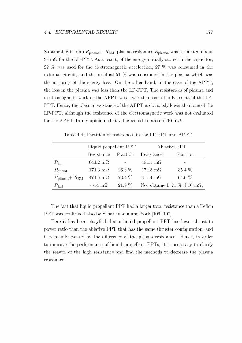
4.4. EXPERIMENTAL RESULTS 177
Subtracting it from Rplasma+ REM, plasma resistance Rplasma was estimated about
33 mΩ for the LP-PPT. As a result, of the energy initially stored in the capacitor,
22 % was used for the electromagnetic acceleation, 27 % was consumed in the
external circuit, and the residual 51 % was consumed in the plasma which was
the majority of the energy loss. On the other hand, in the case of the APPT,
the loss in the plasma was less than the LP-PPT. The resistances of plasma and
electromagnetic work of the APPT was lower than one of only plsma of the LP-
PPT. Hence, the plasma resistance of the APPT is obviously lower than one of the
LP-PPT, although the resistance of the electromagnetic work was not evaluated
for the APPT. In my opinion, that value would be around 10 mΩ.
Table 4.4: Partition of resistances in the LP-PPT and APPT.
Liquid propellant PPT Ablative PPT
Resistance Fraction Resistance Fraction
Rall 64±2 mΩ - 48±1 mΩ -
Rcircuit 17±3 mΩ 26.6 % 17±3 mΩ 35.4 %
Rplasma+ REM 47±5 mΩ 73.4 % 31±4 mΩ 64.6 %
REM ∼14 mΩ 21.9 % Not obtained. 21 % if 10 mΩ,
The fact that liquid propellant PPT had a larger total resistance than a Teflon
PPT was confirmed also by Scharlemann and York [106, 107].
Here it has been claryfied that a liquid propellant PPT has lower thrust to
power ratio than the ablative PPT that has the same thruster configuration, and
it is mainly caused by the difference of the plasma resistance. Hence, in order
to improve the performance of liquid propellant PPTs, it is necessary to clarify
the reason of the high resistance and find the methods to decrease the plasma
resistance.
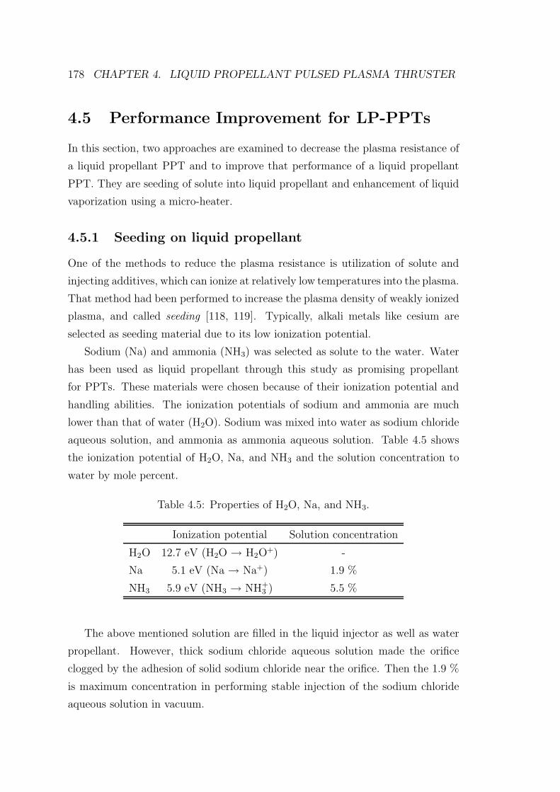
178 CHAPTER 4. LIQUID PROPELLANT PULSED PLASMA THRUSTER
4.5 Performance Improvement for LP-PPTs
In this section, two approaches are examined to decrease the plasma resistance of
a liquid propellant PPT and to improve that performance of a liquid propellant
PPT. They are seeding of solute into liquid propellant and enhancement of liquid
vaporization using a micro-heater.
4.5.1 Seeding on liquid propellant
One of the methods to reduce the plasma resistance is utilization of solute and
injecting additives, which can ionize at relatively low temperatures into the plasma.
That method had been performed to increase the plasma density of weakly ionized
plasma, and called seeding [118, 119]. Typically, alkali metals like cesium are
selected as seeding material due to its low ionization potential.
Sodium (Na) and ammonia (NH3) was selected as solute to the water. Water
has been used as liquid propellant through this study as promising propellant
for PPTs. These materials were chosen because of their ionization potential and
handling abilities. The ionization potentials of sodium and ammonia are much
lower than that of water (H2O). Sodium was mixed into water as sodium chloride
aqueous solution, and ammonia as ammonia aqueous solution. Table 4.5 shows
the ionization potential of H2O, Na, and NH3 and the solution concentration to
water by mole percent.
Table 4.5: Properties of H2O, Na, and NH3.
Ionization potential Solution concentration
H2O 12.7 eV (H2O → H2O+) -
Na 5.1 eV (Na → Na+) 1.9 %
NH3 5.9 eV (NH3 → NH+3 ) 5.5 %
The above mentioned solution are filled in the liquid injector as well as water
propellant. However, thick sodium chloride aqueous solution made the orifice
clogged by the adhesion of solid sodium chloride near the orifice. Then the 1.9 %
is maximum concentration in performing stable injection of the sodium chloride
aqueous solution in vacuum.
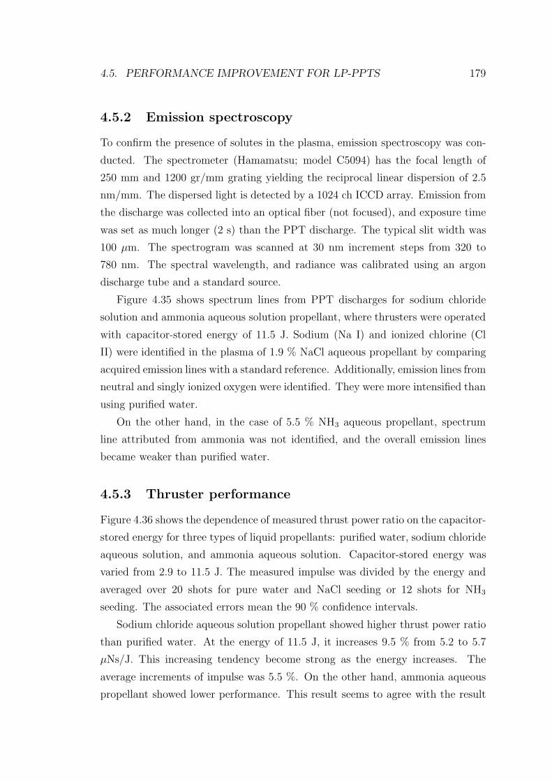
4.5. PERFORMANCE IMPROVEMENT FOR LP-PPTS 179
4.5.2 Emission spectroscopy
To confirm the presence of solutes in the plasma, emission spectroscopy was con-
ducted. The spectrometer (Hamamatsu; model C5094) has the focal length of
250 mm and 1200 gr/mm grating yielding the reciprocal linear dispersion of 2.5
nm/mm. The dispersed light is detected by a 1024 ch ICCD array. Emission from
the discharge was collected into an optical fiber (not focused), and exposure time
was set as much longer (2 s) than the PPT discharge. The typical slit width was
100 µm. The spectrogram was scanned at 30 nm increment steps from 320 to
780 nm. The spectral wavelength, and radiance was calibrated using an argon
discharge tube and a standard source.
Figure 4.35 shows spectrum lines from PPT discharges for sodium chloride
solution and ammonia aqueous solution propellant, where thrusters were operated
with capacitor-stored energy of 11.5 J. Sodium (Na I) and ionized chlorine (Cl
II) were identified in the plasma of 1.9 % NaCl aqueous propellant by comparing
acquired emission lines with a standard reference. Additionally, emission lines from
neutral and singly ionized oxygen were identified. They were more intensified than
using purified water.
On the other hand, in the case of 5.5 % NH3 aqueous propellant, spectrum
line attributed from ammonia was not identified, and the overall emission lines
became weaker than purified water.
4.5.3 Thruster performance
Figure 4.36 shows the dependence of measured thrust power ratio on the capacitor-
stored energy for three types of liquid propellants: purified water, sodium chloride
aqueous solution, and ammonia aqueous solution. Capacitor-stored energy was
varied from 2.9 to 11.5 J. The measured impulse was divided by the energy and
averaged over 20 shots for pure water and NaCl seeding or 12 shots for NH3
seeding. The associated errors mean the 90 % confidence intervals.
Sodium chloride aqueous solution propellant showed higher thrust power ratio
than purified water. At the energy of 11.5 J, it increases 9.5 % from 5.2 to 5.7
µNs/J. This increasing tendency become strong as the energy increases. The
average increments of impulse was 5.5 %. On the other hand, ammonia aqueous
propellant showed lower performance. This result seems to agree with the result
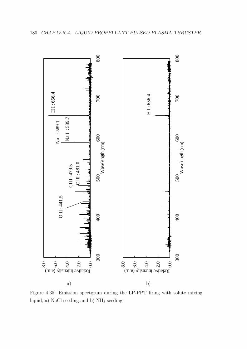
180 CHAPTER 4. LIQUID PROPELLANT PULSED PLASMA THRUSTER
Cl I
I : 4
81.0
Cl I
I : 4
79.5
Na
I : 5
89.1
Na
I :
589.
7
0.0
2.0
4.0
6.0
8.0 30
040
050
060
070
080
0W
avel
engt
h (n
m)
Relative intensity (a.u.)
O I
I : 4
41.5
H I
: 65
6.4
a)
0.0
2.0
4.0
6.0
8.0 30
040
050
060
070
080
0W
avel
engt
h (n
m)
Relative intensity (a.u.)
H I
: 65
6.4
b)
Figure 4.35: Emission spectgrum during the LP-PPT firing with solute mixing
liquid; a) NaCl seeding and b) NH3 seeding.
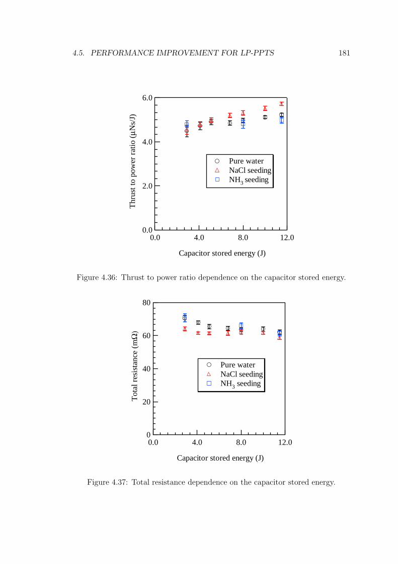
4.5. PERFORMANCE IMPROVEMENT FOR LP-PPTS 181
6.0
4.0
2.0
0.0
Thr
ust t
o po
wer
rat
io (
µNs/
J)
12.08.04.00.0
Capacitor stored energy (J)
Pure water NaCl seeding NH3 seeding
Figure 4.36: Thrust to power ratio dependence on the capacitor stored energy.
80
60
40
20
0
Tot
al r
esis
tanc
e (m
Ω)
12.08.04.00.0
Capacitor stored energy (J)
Pure water NaCl seeding NH3 seeding
Figure 4.37: Total resistance dependence on the capacitor stored energy.
182 CHAPTER 4. LIQUID PROPELLANT PULSED PLASMA THRUSTER
of strong emission lines from NaCl and weak lines for NH3.
Figure 4.37 shows the dependence of total resistance of a liquid propellant
PPT on the energy. It is obtained from the curve-fit of the current waveform,
described in Section 4.3.3. The resistance in Fig. 4.37 shows the average over 20
or 12 shots as well as the thrust power ratio. Sodium chloride aqueous propellant
showed smaller resistance than purified water, whose average decrement was 5.7
%. Ammonia aqueous solution had larger resistance than purified water had.
4.5.4 Discussions on the effect of seeding
For the plasma from sodium chloride aqueous solution, emissions from neutral
sodium and singly ionized chlorine were observed. Ionized sodium and neutral
chlorine were not be observed because they have strong emission lines out of the
range of the spectrometer used here, less than 320 nm and higher than 800 nm
respectively. Presence of those lines means that some fraction of sodium and
chlorine dissolved in water appeared in the plasma.
The results of the impulse and total resistance measurements are consistent
with the relation of the electromagnetic impulse and resistance Eq. 4.24, that is
small total resistance means high thrust to power ratio. Considering the result
of emission spectroscopy, mixing of sodium would increase the plasma density
of liquid propellant PPT. Then the total resistance was decreased. However,
when ammonia mixing in water, the thrust power ratio was decreased against our
expectation. It seems that the plasma density became lower. Some energy might
be excessively consumed for dissociation of the ammonia molecule.
Whereas solute mixing succeeded to decrease the total resistance, it is still 20
% larger than a Teflon PPT. Two reasons are considered. Firstly, solutes had
only slight effect on the increment of plasma density. Secondly, plasma density
was already high but the low electron temperature caused the high resistance
(electrical conductivity in fully ionized plasma is proportional to and does not
depend on the plasma density). Quantitative measurements for plasma density
and temperature are required to clarify those processes.
4.5. PERFORMANCE IMPROVEMENT FOR LP-PPTS 183
4.5.5 Enhancement of water vaporization
High resistance of a water propellant PPT can be caused by low propellant den-
sity in interelectrode space. It would be not liquid droplets themselves but the
evaporated gas which directly contributes to plasma. It is uncertain that how
quantity of gas exists before the firing in the interelectrode of a liquid propellant
PPT. However, the high plasma velocity observed in Section 4.4.4 indicated the
low plasma density. In this section, injecting liquid droplets on a microheater is
examined to increase the gaseous propellant density, or pressure, and to decrease
the plasma resistance.
Estimation of water droplets evaporation
First, evaporation rate of liquid droplets is estimated. There are the following
two evaporation processes of liquid ejected in vacuum: evaporation of flying liquid
droplets by the own heat capacity and evaporation of liquid adhering on walls by
heat conduction from the walls.
Droplets ejected into the vacuum evaporate by their own heat. The evaporation
mass flux: Γm is expressed as
Γm =
√M
2πRTPvapor(T ) (4.34)
where Pvapor is the vapor pressure of liquid. Return of evaporated gas from the
vicinity of the liquid droplets was neglected. Generally vapor pressure has large
dependence on the temperature as shown in Fig. 4.38 and the evaporation is
suppressed by decrease of temperature due to its latent heat.
For instance, water droplets of 5 µg has the total surface area of 1.2 mm2
provided that all droplets have the same diameter of 25 µm. They have the
evaporation rate of 3.0 µg/ms at 293 K and 0.4 µg/ms at 263 K. Then flying
droplets is rapidly cooled and the evaporation is almost stopped within a few mili
second. According to the calculation, only 20 % of the mass will be evaporated
within 5 ms and the most is evaporated within 0.5 ms.
Droplets adhering on a wall can obtain heat from the wall and can keep to
evaporate. In this case, the characteristic time of evaporation is determined by
the heat conduction of both the wall and droplets. The heat penetration depth:
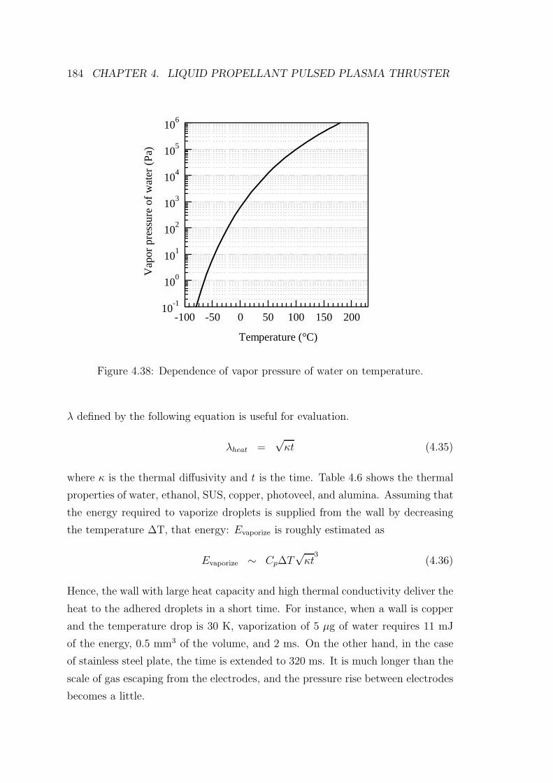
184 CHAPTER 4. LIQUID PROPELLANT PULSED PLASMA THRUSTER
10-1
100
101
102
103
104
105
106
Vap
or p
ress
ure
of w
ater
(P
a)
200150100500-50-100
Temperature (°C)
Figure 4.38: Dependence of vapor pressure of water on temperature.
λ defined by the following equation is useful for evaluation.
λheat =√
κt (4.35)
where κ is the thermal diffusivity and t is the time. Table 4.6 shows the thermal
properties of water, ethanol, SUS, copper, photoveel, and alumina. Assuming that
the energy required to vaporize droplets is supplied from the wall by decreasing
the temperature ∆T, that energy: Evaporize is roughly estimated as
Evaporize ∼ Cp∆T√
κt3
(4.36)
Hence, the wall with large heat capacity and high thermal conductivity deliver the
heat to the adhered droplets in a short time. For instance, when a wall is copper
and the temperature drop is 30 K, vaporization of 5 µg of water requires 11 mJ
of the energy, 0.5 mm3 of the volume, and 2 ms. On the other hand, in the case
of stainless steel plate, the time is extended to 320 ms. It is much longer than the
scale of gas escaping from the electrodes, and the pressure rise between electrodes
becomes a little.
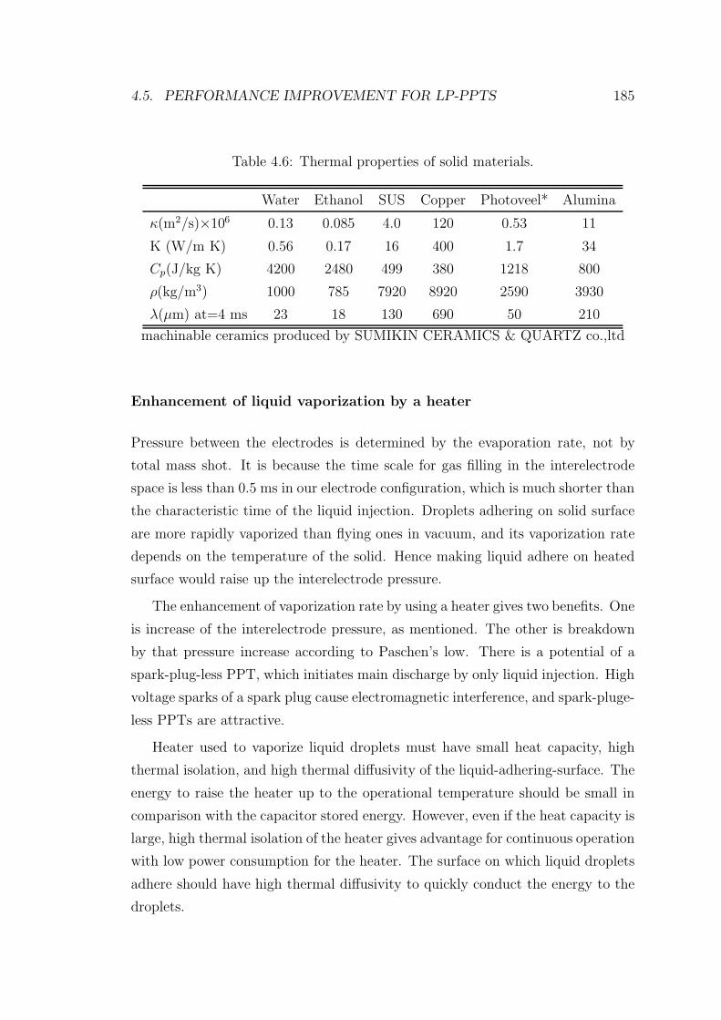
4.5. PERFORMANCE IMPROVEMENT FOR LP-PPTS 185
Table 4.6: Thermal properties of solid materials.
Water Ethanol SUS Copper Photoveel* Alumina
κ(m2/s)×106 0.13 0.085 4.0 120 0.53 11
K (W/m K) 0.56 0.17 16 400 1.7 34
Cp(J/kg K) 4200 2480 499 380 1218 800
ρ(kg/m3) 1000 785 7920 8920 2590 3930
λ(µm) at=4 ms 23 18 130 690 50 210
machinable ceramics produced by SUMIKIN CERAMICS & QUARTZ co.,ltd
Enhancement of liquid vaporization by a heater
Pressure between the electrodes is determined by the evaporation rate, not by
total mass shot. It is because the time scale for gas filling in the interelectrode
space is less than 0.5 ms in our electrode configuration, which is much shorter than
the characteristic time of the liquid injection. Droplets adhering on solid surface
are more rapidly vaporized than flying ones in vacuum, and its vaporization rate
depends on the temperature of the solid. Hence making liquid adhere on heated
surface would raise up the interelectrode pressure.
The enhancement of vaporization rate by using a heater gives two benefits. One
is increase of the interelectrode pressure, as mentioned. The other is breakdown
by that pressure increase according to Paschen’s low. There is a potential of a
spark-plug-less PPT, which initiates main discharge by only liquid injection. High
voltage sparks of a spark plug cause electromagnetic interference, and spark-pluge-
less PPTs are attractive.
Heater used to vaporize liquid droplets must have small heat capacity, high
thermal isolation, and high thermal diffusivity of the liquid-adhering-surface. The
energy to raise the heater up to the operational temperature should be small in
comparison with the capacitor stored energy. However, even if the heat capacity is
large, high thermal isolation of the heater gives advantage for continuous operation
with low power consumption for the heater. The surface on which liquid droplets
adhere should have high thermal diffusivity to quickly conduct the energy to the
droplets.
186 CHAPTER 4. LIQUID PROPELLANT PULSED PLASMA THRUSTER
Microheater assembly
A commercially available microheater was used to heat up solid surface receiving
liquid droplets. It consists of platinum thin film photo-ithographically structured
on a 0.15 mm thick alumina substrate. The microheater was bound on a copper
main body by Torr Seal r©with thermocouple lines. The main body consists of
a circular plate with 0.8 mm thickness and 3.7 mm diameter and a rectangular
plate with 3.7 mm width, 11mm length, 0.6 mm thickness. Liquid droplets is
ejected toward the surface of the circular plate. The copper body was surrounded
by a shell made of photoveel. The glued component, a microheater, copper main
body, thermocouple lines, and photoveel shell, is referred as a microheater assem-
bly, which is shown in Fig. 4.39. Only the top of the ceramic shell is fixed to
the electrode, to avoid the electrical coupling to electrode and insulate from the
electrode.
φ5.0
φ 3.7
12
Heater
Thermocouple
Copper
Ceramic
Torr seal
0.8
0.6
0.35
Heater
Copper bodyCopper body
Thermocouple
a) b)
φ5.0
φ 3.7
12
Heater
Thermocouple
Copper
Ceramic
Torr seal
0.8
0.6
0.35
Heater
Copper bodyCopper body
Thermocouple
a) b)
Figure 4.39: Microheater assembly. a) schematic drawing of a microheater assem-
bly and b) photograph before the gluing.
Temperature of the microheater was controlled to be constant using a set
point controller. The temperature was measured using a monolithic thermocouple
conditioner from Analog Devices (AD597). The temperature output was compared
4.5. PERFORMANCE IMPROVEMENT FOR LP-PPTS 187
to the set-point temperature and a switching circuit of the heater was controlled.
That electrical diagram is shown in Appendix F. The temperature was ranged
from 20 to 100 C. The maximum temperature was restricted by the temperature
limit of the glue dealt here, Torr Seal.
Designed LP-PPTs with using a microheater.
Two varieties of LP-PPTs were designed to enhance the vaporization rate of liquid
droplets using the microheater assembly. Those schematic diagrams are shown in
Fig. 4.40. Both LP-PPTs have no spark plug and initiate discharge by breakdown
by raising the interelectrode pressure.
Figure 4.40 a) is referred as single discharge LP-PPT and Fig. 4.40 b) is referred
as double discharge LP-PPT. The first, single discharge LP-PPT, has two parts
of parallel plate electrodes as shown in the figure: ignition part and acceleration
part. Ignition part has the narrow interelectrode distance of 1 mm and the length
of 12 mm. Following the ignition part, acceleration part has the electrodes of 20
mm distance and 35 mm length (cathode is 57 mm). These electrodes are made
of copper plates with the thickness of 2 mm.
The ignition part is designed to effectively raise the interelectrode pressure.
The microheater assembly is installed 4 mm away from the back wall on the anode.
Injection hole for liquid droplets was aligned along the center of the receive plate of
the microheater. The ejected liquid droplets exactly hit on the plate because of the
short interelectrode distance. Moreover the short distance decreases conductance
of the channel. Thin parallel plates channel has the following conductance for
rarefied gas stream[120].
Cparallel = 116 ln(l/d)wd2
l(m3/s) for l/d > 10 (4.37)
where d is the distance between the plates, l is the length, and w is the width.
Therefore the electrode distance quadratically decreases the conductance.
The acceleration part is designed to effectively accelerate the plasma by elec-
tromagnetic force. The inductance per unit length: L′ for a rectangle circuit with
parallel plates is given by Eq. 4.29. According to that equation, the acceleration
electrodes have L′ of 0.8 nH/mm. For the ignition part, Eq. 4.29 cannot be ap-
plied due to its too narrow distance. Instead, L′ for two dimensional case can be
used: µ0d/w. Then ignition part has the L′ of 0.13 nH/mm.
188 CHAPTER 4. LIQUID PROPELLANT PULSED PLASMA THRUSTER
12
1
4
Anode
Cathode
Side walls (glass)
Main capacitor(3 µ F)
Microheater
Back wall (ceramic)
Electrode width: 10
Microheater
e
a)
b)
12.51
Anode
Cathode
Main capacitor(3 µ F)
Ignition capacitor (25 nF)
Ignition anode
Liquid injectorInjection hole
20
Heater plate
Liquid droplets
Magnified view
Second back wall(ceramic)
Figure 4.40: Schematic diagrams of the LP-PPT using the microheater.
4.5. PERFORMANCE IMPROVEMENT FOR LP-PPTS 189
The double discharge LP-PPT has two capacitors as shown in Fig. 4.40 b),
main capacitor of 3 µF and ignition capacitor of 25 nF. Whereas it has two parts
as well as the single discharge LP-PPT, anodes of those parts are electrically sep-
arated and respectively connected to the capacitors. This design is motivated to
prevent the energy excessively consumed in the ignition part. Because the igni-
tion part has lower L′ than typical PPTs, discharge current passing there hardly
contributes to the acceleration. Small discharge plasma generated in ignition part
induces main discharge between main electrodes. After all the ignition part be-
haves similar to a spark plug. The advantages over a spark plug are that there is
no need of high voltage for the discharge, because the breakdown occurs automat-
ically when the pressure reaches up to the certain value.
Another benefit of the double discharge LP-PPT is to use low voltage for the
charge of a main capacitor. The single discharge LP-PPT requires high voltage
enough to make breakdown. Therefore it restricts the capacitor applied voltage.
On the other hand, in the double discharge LP-PPT, the voltage of the main ca-
pacitor can be set under the breakdown voltage, and only the ignition capacitor
requires higher voltage. Thus the capacitor stored energy can be widely ranged
from low level. In this study, 3.0 kV was constantly applied to the ignition capac-
itor and the voltage applied to the main capacitance was ranged from 1.5 to 3.0
kV.
4.5.6 Experimental results of PPT using a microheater
Operation.
First, the ignition probability was investigated using a heater for the enhancement
of the liquid vaporization. A parallel plate electrode with only ignition part was
used to clarify the threshold. The voltage of 3 kV was applied the electrode and
the liquid was ejected on the heater assembly. The temperature and mass shot of
the liquid was changed.
At the standard temperature around 20 C, there was no breakdown by inject-
ing water droplets of 20 µg. Increasing the temperature, breakdown occured by
less liquid injection, and at 100 C it was accomplished by 6 µg liquid injection.
In less mass shot of 4 to 6 µg, the breakdown was accomplished in several times
at the heater temperature of 100 C. Under the 4 µg of mass shot, no breakdown
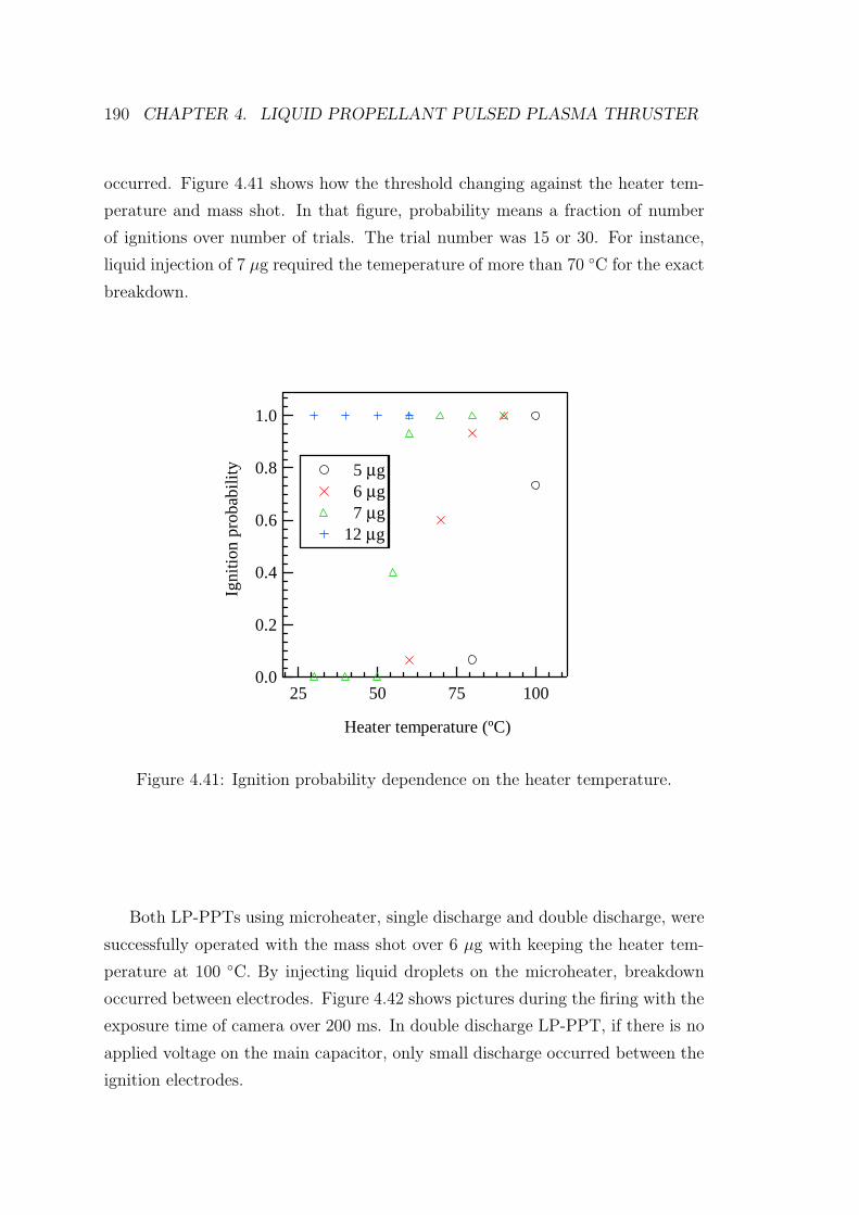
190 CHAPTER 4. LIQUID PROPELLANT PULSED PLASMA THRUSTER
occurred. Figure 4.41 shows how the threshold changing against the heater tem-
perature and mass shot. In that figure, probability means a fraction of number
of ignitions over number of trials. The trial number was 15 or 30. For instance,
liquid injection of 7 µg required the temeperature of more than 70 C for the exact
breakdown.
1.0
0.8
0.6
0.4
0.2
0.0
Igni
tion
prob
abili
ty
100755025
Heater temperature (ºC)
5 µg 6 µg 7 µg12 µg
Figure 4.41: Ignition probability dependence on the heater temperature.
Both LP-PPTs using microheater, single discharge and double discharge, were
successfully operated with the mass shot over 6 µg with keeping the heater tem-
perature at 100 C. By injecting liquid droplets on the microheater, breakdown
occurred between electrodes. Figure 4.42 shows pictures during the firing with the
exposure time of camera over 200 ms. In double discharge LP-PPT, if there is no
applied voltage on the main capacitor, only small discharge occurred between the
ignition electrodes.
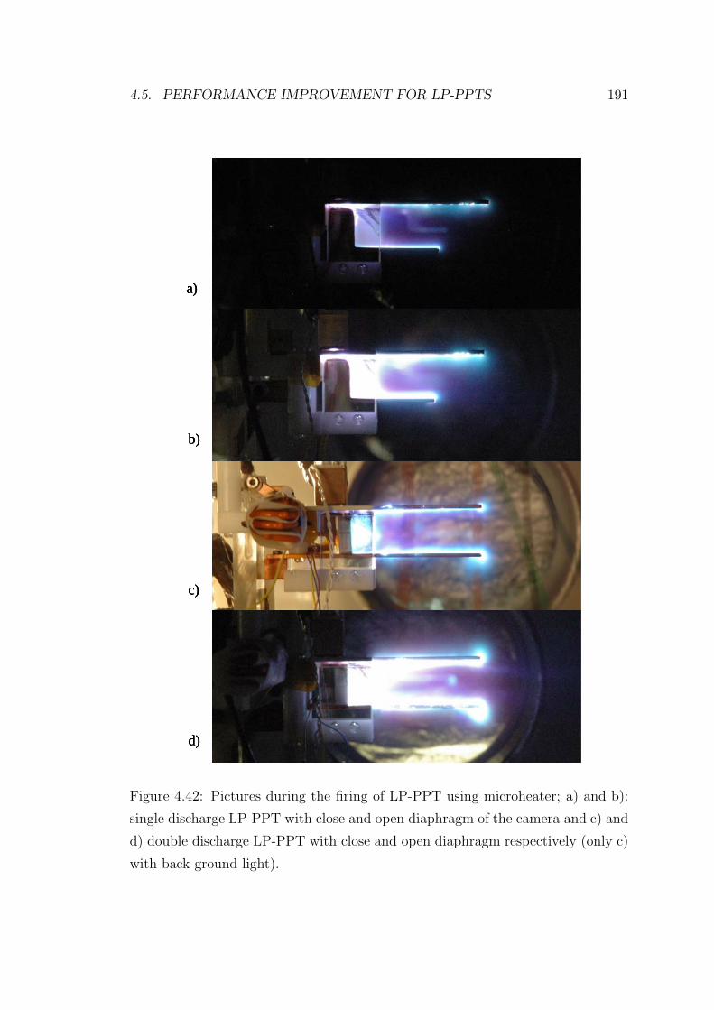
4.5. PERFORMANCE IMPROVEMENT FOR LP-PPTS 191
a)
b)
c)
d)
a)
b)
c)
d)
a)
b)
c)
d)
Figure 4.42: Pictures during the firing of LP-PPT using microheater; a) and b):
single discharge LP-PPT with close and open diaphragm of the camera and c) and
d) double discharge LP-PPT with close and open diaphragm respectively (only c)
with back ground light).
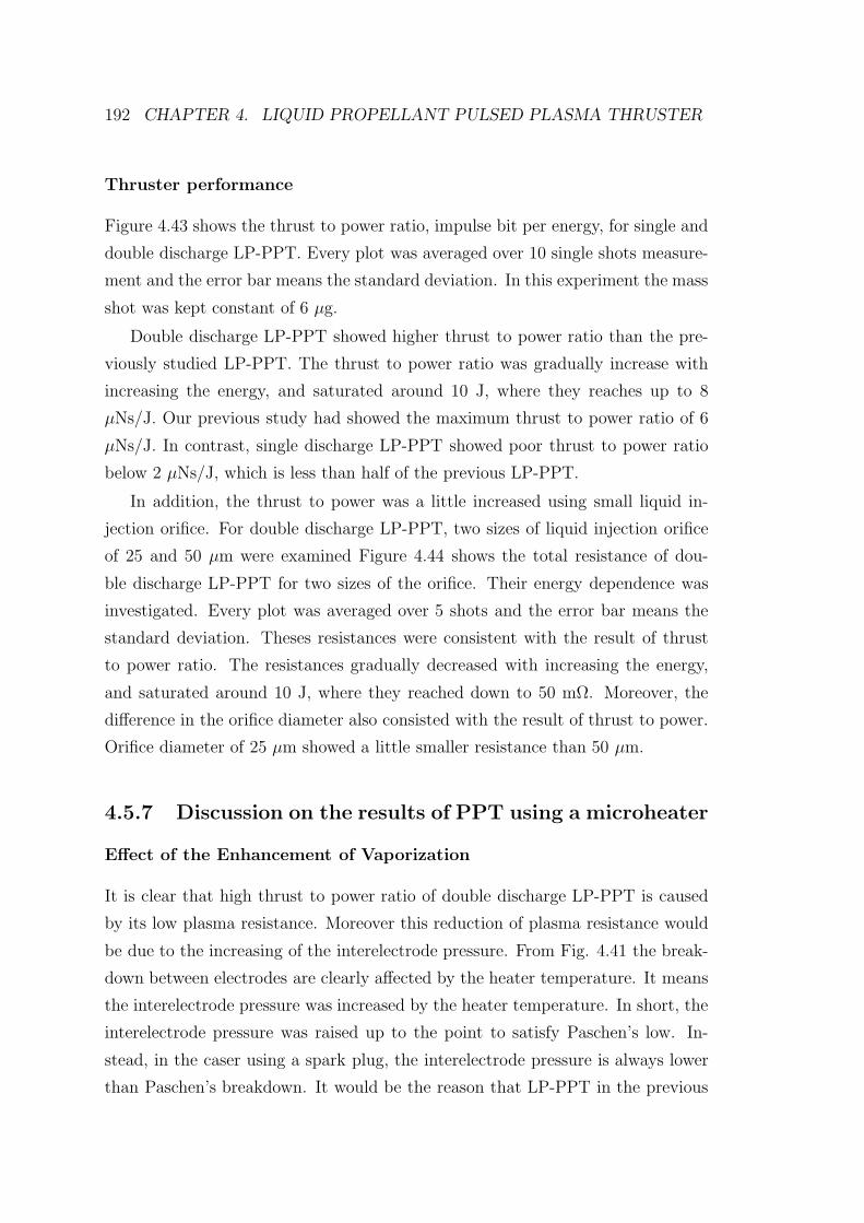
192 CHAPTER 4. LIQUID PROPELLANT PULSED PLASMA THRUSTER
Thruster performance
Figure 4.43 shows the thrust to power ratio, impulse bit per energy, for single and
double discharge LP-PPT. Every plot was averaged over 10 single shots measure-
ment and the error bar means the standard deviation. In this experiment the mass
shot was kept constant of 6 µg.
Double discharge LP-PPT showed higher thrust to power ratio than the pre-
viously studied LP-PPT. The thrust to power ratio was gradually increase with
increasing the energy, and saturated around 10 J, where they reaches up to 8
µNs/J. Our previous study had showed the maximum thrust to power ratio of 6
µNs/J. In contrast, single discharge LP-PPT showed poor thrust to power ratio
below 2 µNs/J, which is less than half of the previous LP-PPT.
In addition, the thrust to power was a little increased using small liquid in-
jection orifice. For double discharge LP-PPT, two sizes of liquid injection orifice
of 25 and 50 µm were examined Figure 4.44 shows the total resistance of dou-
ble discharge LP-PPT for two sizes of the orifice. Their energy dependence was
investigated. Every plot was averaged over 5 shots and the error bar means the
standard deviation. Theses resistances were consistent with the result of thrust
to power ratio. The resistances gradually decreased with increasing the energy,
and saturated around 10 J, where they reached down to 50 mΩ. Moreover, the
difference in the orifice diameter also consisted with the result of thrust to power.
Orifice diameter of 25 µm showed a little smaller resistance than 50 µm.
4.5.7 Discussion on the results of PPT using a microheater
Effect of the Enhancement of Vaporization
It is clear that high thrust to power ratio of double discharge LP-PPT is caused
by its low plasma resistance. Moreover this reduction of plasma resistance would
be due to the increasing of the interelectrode pressure. From Fig. 4.41 the break-
down between electrodes are clearly affected by the heater temperature. It means
the interelectrode pressure was increased by the heater temperature. In short, the
interelectrode pressure was raised up to the point to satisfy Paschen’s low. In-
stead, in the caser using a spark plug, the interelectrode pressure is always lower
than Paschen’s breakdown. It would be the reason that LP-PPT in the previous
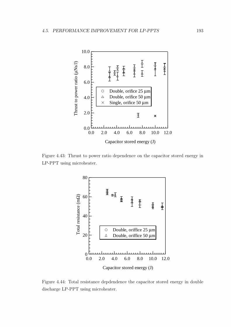
4.5. PERFORMANCE IMPROVEMENT FOR LP-PPTS 193
10.0
8.0
6.0
4.0
2.0
0.0
Thr
ust t
o po
wer
rat
io (
µNs/
J)
12.010.08.06.04.02.00.0
Capacitor stored energy (J)
Double, orifice 25 µm Double, orifice 50 µm Single, orifice 50 µm
Figure 4.43: Thrust to power ratio dependence on the capacitor stored energy in
LP-PPT using microheater.
80
60
40
20
0
Tot
al r
esis
tanc
e (m
Ω)
12.010.08.06.04.02.00.0
Capacitor stored energy (J)
Double, oriffice 25 µm Double, oriffice 50 µm
Figure 4.44: Total resistance depdendence the capacitor stored energy in double
discharge LP-PPT using microheater.
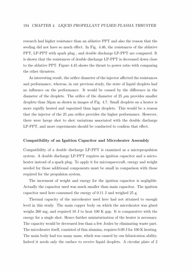
194 CHAPTER 4. LIQUID PROPELLANT PULSED PLASMA THRUSTER
research had higher resistance than an ablative PPT and also the reason that the
seeding did not have so much effect. In Fig. 4.46, the resistances of the ablative
PPT, LP-PPT with spark plug , and double discharge LP-PPT are compared. It
is shown that the resistances of double discharge LP-PPT is decreased down close
to the ablative PPT. Figure 4.45 shows the thrust to power ratio with comparing
the other thrusters.
As interesting result, the orifice diameter of the injector affected the resistances
and performance, whereas, in our previous study, the state of liquid droplets had
no influence on the performance. It would be caused by the difference in the
diameter of the droplets. The orifice of the diameter of 25 µm provides smaller
droplets than 50µm as shown in images of Fig. 4.7. Small droplets on a heater is
more rapidly heated and vaporized than lager droplets. This would be a reason
that the injector of the 25 µm orifice provides the higher performance. However,
there were larege shot to shot variations associated with the double discharge
LP-PPT, and more experiments should be conducted to confirm that effect.
Compatibility of an Ignition Capacitor and Microheater Assembly
Compatibility of a double discharge LP-PPT is examined as a micropropulsion
system. A double discharge LP-PPT requires an ignition capacitor and a micro-
heater instead of a spark plug. To apply it for microspacecraft, energy and weight
needed for those additional components must be small in comparison with those
required for the propulsion system.
The increment of weight and energy for the ignition capacitor is negligible.
Actually the capacitor used was much smaller than main capacitor. The ignition
capacitor used here consumed the energy of 0.11 J and weighed 25 g.
Thermal capacity of the microheater used here had not attained to enough
level in this study. The main copper body on which the microheater was glued
weighs 260 mg, and required 10 J to heat 100 K gap. It is comparative with the
energy for a single shot. Hence further miniaturization of the heater is necessary.
The capacity would be decreased less than a few Joules by eliminating waste part.
The microheater itself, consisted of thin alumina, requires 0.09 J for 100 K heating.
The main body had too many mass, which was caused by our fabarication ability.
Indeed it needs only the surface to receive liquid droplets. A circular plate of 2
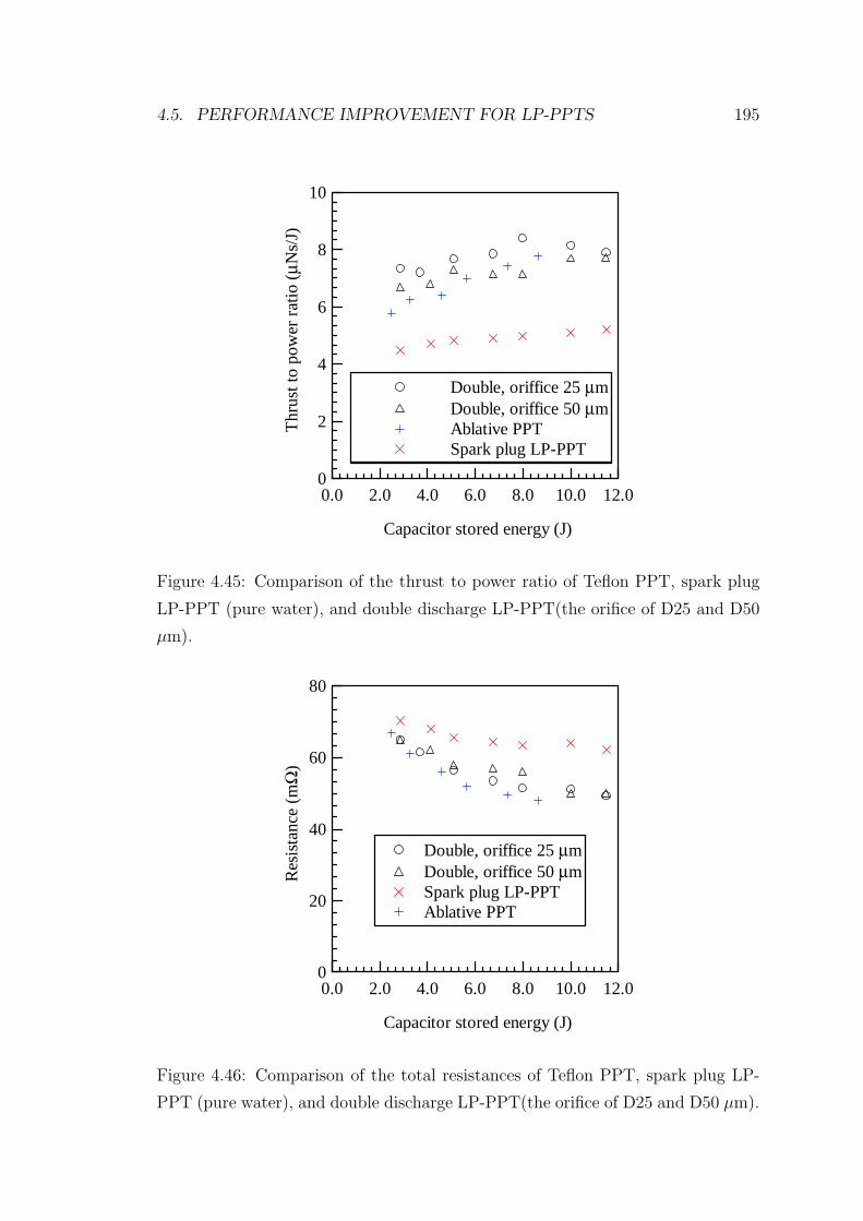
4.5. PERFORMANCE IMPROVEMENT FOR LP-PPTS 195
10
8
6
4
2
0
Thr
ust t
o po
wer
rat
io (
µNs/
J)
12.010.08.06.04.02.00.0
Capacitor stored energy (J)
Double, oriffice 25 µm Double, oriffice 50 µm Ablative PPT Spark plug LP-PPT
Figure 4.45: Comparison of the thrust to power ratio of Teflon PPT, spark plug
LP-PPT (pure water), and double discharge LP-PPT(the orifice of D25 and D50
µm).
80
60
40
20
0
Res
ista
nce
(mΩ
)
12.010.08.06.04.02.00.0
Capacitor stored energy (J)
Double, oriffice 25 µm Double, oriffice 50 µm Spark plug LP-PPT Ablative PPT
Figure 4.46: Comparison of the total resistances of Teflon PPT, spark plug LP-
PPT (pure water), and double discharge LP-PPT(the orifice of D25 and D50 µm).
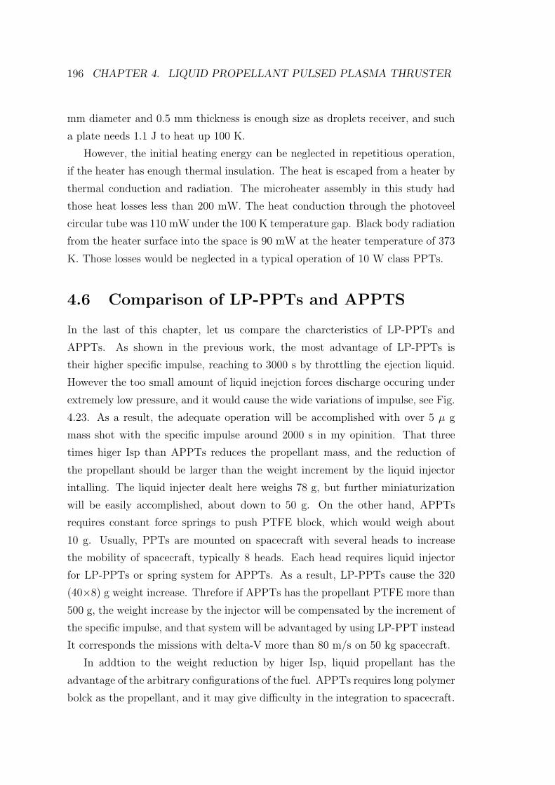
196 CHAPTER 4. LIQUID PROPELLANT PULSED PLASMA THRUSTER
mm diameter and 0.5 mm thickness is enough size as droplets receiver, and such
a plate needs 1.1 J to heat up 100 K.
However, the initial heating energy can be neglected in repetitious operation,
if the heater has enough thermal insulation. The heat is escaped from a heater by
thermal conduction and radiation. The microheater assembly in this study had
those heat losses less than 200 mW. The heat conduction through the photoveel
circular tube was 110 mW under the 100 K temperature gap. Black body radiation
from the heater surface into the space is 90 mW at the heater temperature of 373
K. Those losses would be neglected in a typical operation of 10 W class PPTs.
4.6 Comparison of LP-PPTs and APPTS
In the last of this chapter, let us compare the charcteristics of LP-PPTs and
APPTs. As shown in the previous work, the most advantage of LP-PPTs is
their higher specific impulse, reaching to 3000 s by throttling the ejection liquid.
However the too small amount of liquid inejction forces discharge occuring under
extremely low pressure, and it would cause the wide variations of impulse, see Fig.
4.23. As a result, the adequate operation will be accomplished with over 5 µ g
mass shot with the specific impulse around 2000 s in my opinition. That three
times higer Isp than APPTs reduces the propellant mass, and the reduction of
the propellant should be larger than the weight increment by the liquid injector
intalling. The liquid injecter dealt here weighs 78 g, but further miniaturization
will be easily accomplished, about down to 50 g. On the other hand, APPTs
requires constant force springs to push PTFE block, which would weigh about
10 g. Usually, PPTs are mounted on spacecraft with several heads to increase
the mobility of spacecraft, typically 8 heads. Each head requires liquid injector
for LP-PPTs or spring system for APPTs. As a result, LP-PPTs cause the 320
(40×8) g weight increase. Threfore if APPTs has the propellant PTFE more than
500 g, the weight increase by the injector will be compensated by the increment of
the specific impulse, and that system will be advantaged by using LP-PPT instead
It corresponds the missions with delta-V more than 80 m/s on 50 kg spacecraft.
In addtion to the weight reduction by higer Isp, liquid propellant has the
advantage of the arbitrary configurations of the fuel. APPTs requires long polymer
bolck as the propellant, and it may give difficulty in the integration to spacecraft.
4.6. COMPARISON OF LP-PPTS AND APPTS 197
Figure 4.47: Dawgstar APPT desinged in University of Washington.
Typical 10 J class APPTs has the 2 cm2 cross section of PTFE bolck. It means
100 g PTFE block has the length of about 25 cm (the density of PTFE is about
2 g/cm3). Figure 4.47 shows an APPT designed in Univesity of Washington for
Dawgstar satellite[115]. If much more propellant is needed, the longer PTFE block
may conflict with the other spacecraft hardwares.
Moreover, other advantages of using liquid propellant are avoinding non uni-
form ablation of the polymer and use of no charring or toxic material. The polymer
material is likely to attach on solid walls of thruster and spacecraft rather than
liquid propellant. On the contrary, disadvantages of liquid propellant are risks of
leaking and clogging of liquid. Additionally, water has the capability of icing in
sapce. The use of heater to melt the ice will increase a lot of power. In terms of
stabel propellant selection, alcohol propellant is attractive. Previous work on liq-
uid propellant PPTs showed the successful operation using ethanol and methanol
propellant with the equivalent performance.
198 CHAPTER 4. LIQUID PROPELLANT PULSED PLASMA THRUSTER
4.7 Conclusion of Chapter 4
In this chapter, a liquid pulsed plasma thruster was investigated and its perfor-
mance improvement methods were proposed, and the following conclusions were
obtained.
• Energy partitions in a liquid propellant PPT was evaluated. Of the energy,
22 % was used as the electromagnetic acceleration of plasma, 27% was con-
sumed as the energy loss in the external circuit was 27 %, and 51 % was
consumed in the plasma. The energy loss in the plasma was higher than one
of the ablative PPT with the same configuration. As a result, lower thrust
power ratio using water was caused by the higher plasma resistance than
using PFFE.
• Seeding sodium chloride in water decreased the plasma resistance and in-
creased the thrust by 5.5 %. Emission spectrum from discharge plasma was
also strengthened by the seeding. In contrast, ammonia seeding showed no
a little decrease of the thrust.
• Liquid vaporization rate was enhanced using a micro heater and it enabled
breakdown by the pressure rising injecting 6 µg water droplets.
• The enhanced water vaporization increased the thrust by 30 % with dou-
ble discharge mode. It was because that the interelectrode pressure was
increased by enhancing the water vaporization.
Chapter 5
Conclusions
This study has been performed to propose and develop micropropulsions suited
with 1 - 00 kg microspacecraft. In order to reach to the goal, the following studies
were conducted. First, a high accuracy thrust stand was developed to exactly
evaluate the performance of micropropulsions. Secondly, a dual propulsive mode
laser microthruster was proposed for microspacecraft less than 10 kg and the
fundamental characteristics were clarified. A pulsed plasma thruster using liquid
was investigated for microspacecraft over 10 kg by clarifying energy partitions,
and the performance improvements were conducted. The major conclusions of
this study are:
Thrust stand for micropropulsions
• A thrust stand with high resolution and accuracy was developed. The reso-
lution was less than 1.0 µNs and the accuracy is within 2.0 %. That thrust
measurement was examined using thrusters of the weight up to 2.0 kg (the
stand was designed to endure thruster weight over 10 kg).
• Tight adjustment of the gravity center (<10 µ m) and effective damping of
the stand enabled the high resolution and high usability.
• A curve-fitting method was newly proposed to removing the mechanical
noises induced by background vibrations. That effect was analytically clar-
ified and experimentally verified.
199
200 CHAPTER 5. CONCLUSIONS
Dual propulsive mode laser microthruster
• The successful operation of laser ablation mode was verified using polyvinyl
chloride propellant. The thrust provided by the laser ablation was propor-
tional to the laser pulse width with the thrust to power ratio of 40 to 150
µNs/J according to the ablative material. It enabled the laser ablation mode
to provide lower thrust with high resolution.
• Absorption rate of the ablative propellant strongly affected the thrust perfor-
mance, especially thrust to power ratio. Polyvinyl chloride with rich carbon
density showed higher thrust to power ratio.
• Laser ignited combustion of pyrotechnic in vacuum was verified using boron /
potassium nitrate. The laser ignition processes of Boron / potassium nitrate
was well reproduced with numerical calculation, where three dimensional
heat conduction problem was solved with the exothermic reaction.
• The threshold laser power and pulse with for the laser ignition was adequate
for the use of microspacecraft, 300 mW and 150 ms. That laser ignited
combustion enabled laser microthruster to provide higher thrust of 11 mNs
and 600 mNs according to the size of the pyrotechnics.
Pulsed plasma thruster using liquid propellant
• Energy partitions of a liquid propellant pulsed plasma thruster was evaluated
and the most energy loss was the dissipation in the plasma (51 %). It
was revealed that the higher plasma resistance when using liquid propellant
caused the low thrust power.
• Seeding sodium chloride in water decreased the plasma resistance and in-
creased the thrust by 5.5 %. Emission spectrum from discharge plasma was
also strengthened by the seeding. In contrast, ammonia seeding showed no
a little decrease of the thrust.
• Liquid vaporization was enhanced using a micro heater and it enabled break-
down by the pressure rise with the adequate mass shot. The enhanced water
vaporization increased the thrust by 30 % with a double discharge mode. It
was because of the increased interelectrode pressure.
References
[1] M. M. Micci and A. D. Ketsdever, editors. Micropropulsion for Small Space-
craft, volume 187 of Progress in Astronautics and Aeronautics. American
Institute of Aeronautics and Astornautics, Inc., 2000.
[2] Y. Nojiri, M. Nagai, Y. Nakamura, R. Funase, T. Eishima, E. Takei, C. Yu-
liang, A. Enokuchi, K. Nakada, and S. Nakasuka. University of tokyo’s nano-
satellite cubesat-xi and its on-orbit experiment results. In 24thInternational
Symposium on Space Science and Technology, Miyazaki, Japan, 2004. ISTS
2004-f-05.
[3] C. Kitts, R. Twiggs, F. Pranajaya, B. Palmintier, and J. How. Emerald:
a low-cost spacecraft mission for validating formation flying technologies.
1999 IEEE Aerospace Conference Proceedings, 2, pp.217–226, 1999.
[4] A. Valdez, C. Hu, C. Kitts, M. Breiling, A. Slaughterbeck, J. Ota, D.
Hadi, T. Kuhlman, and S. Lyons. The artemis project: Picosatellites and
the feasibility of the smaller, faster, cheaper approach. 1999 IEEE Aerospace
Conference Proceedings, 2, pp.235–243, 1999.
[5] S.C. Solomon, S.M. Bailey, C.A. Barth, R.L. Davis, J.A. Donnelly, T.E.
Holden, M.S. Kelley, R.A. Kohnert, M.T. McGrath, A.W. Merkel, H.L.
Reed, S.M. Ryan, M.A. Salada, S.R. Steg, G.A. Tate, J.C. Westfall, J.J.
Westphal, and P.R. Withnell. The snoe spacecraft: Integration, test, launch,
operation, and on-orbit performance. In Proceedings of the 12th Annual
AIAA/USU Conference on Small Satellites, Logan, Utah, USA, 1998. ISTS
2004-f-05.
201
202 REFERENCES
[6] K. T. Alfriend, S. R. Vadali, and H. Schaub. Formation flying satellites:
Control by an astrodynamicist. Celestial Mechanics and Dynamical Astron-
omy, 81, pp.57–62, 2001.
[7] C. Sabol, R. Burns, and C. A. McLaughlin. Satellite formation flying design
and evolution. Journal of Spacecraft and Rocket, 38(2), pp.270–278, 2001.
[8] R. S. Smith and F. Y. Hadaegh. Control of deep-space formation-flying
spacecraft; relative sensing and switched information. Journal of Guidance,
Control, and Dynamics, 28(1), pp.106–114, 2005.
[9] W. Ren and R. W. Beard. Decentralized scheme for spacecraft formation
flying via the virtual structure approach. Journal of Guidance, Control, and
Dynamics, 27(1), pp.73–82, 2004.
[10] P. R. Lawson. The terrestrial planet finder. 2001 IEEE Aerospace Conference
Proceedings, 4, pp.2005–2011, 2001.
[11] C. V. M. Fridlund. Darwin - the infrared space interferometry mission. ESA
Bulletin, 103, pp.20–25, 2000.
[12] K. Danzmann and LISA Study Team. Lisa: laser interferometer space an-
tenna for the detection and observation of gravitational waves. In 2nd ed.,
Max-Planck Inst. fur Quantenoptik, Garching, Germany, 1998. ISTS 2004-
f-05.
[13] S. Nakasuka. Requirement for microthruster. Private meeting with Nakasuka
lab in University of Tokyo, 2004.
[14] M. Nakano. Mission using electric propulsions. In K. Kuriki and Y. Arakawa,
editors, Introduction to Electric Propulsion, chapter 10. University of Tokyo
Press, 2003.
[15] J. Muller. Thruster options for microspacecraft: A review and evaluation of
evaluation of state-of-the-art and emerging technologies. In M. M. Micci and
A. D. Ketsdever, editors, Micropropulsion for Small Spacecraft, volume 187
of Progress in Astronautics and Aeronautics, chapter 3. American Institute
of Aeronautics and Astornautics, Inc., 2000.
REFERENCES 203
[16] A. P. London, A. H. Epstein, and J. L. Kerrebrock. High-pressure bipropel-
lant microrocket engine. Journal of Propulsion and Power, 17(4), pp.780–
787, 2001.
[17] D. H. Lewis, S. W. Janson, R. B. Cohen, and E. K. Antonsson. Digital
micropropulsion. Sensors and Actuators, 80, pp.143–154, 2000.
[18] C. Rossi, T. D. Conto, D. Esteve, and B. Larangot. Design, fabrication
and modeling of mems-based microthrusters for space application. Smart
Materials and Structures, 10(6), pp.1156–1162, 2001.
[19] S. Tanaka, R. Hosokawa, S. Tokudome, K. Hori, H. Saito, M. Watanabe, and
M. Esashi. Mems-based solid propellant rocket array thruster. Transactions
of the Japan Society for Aeronautical and Space Sciences, 46(151), pp.47–51,
2003.
[20] K. L. Zhang, S. K. Chou, and S. S. Ang. Development of a solid propellant
microthruster with chamber and nozzle etched on a wafer surface. Journal
of Micromechanics and Microengineering, 14, pp.785–792, 2004.
[21] R. G. Jahn. Physics of Electric Propulsion. McGraw-Hill, New York, 1968.
[22] K. Kuriki and Y. Arakawa, editors. Introduction to Electric Propulsion.
University of Tokyo Press, 2003.
[23] A. Sengupta, J. Brophy, J. Anderson, and C. Garner. An overview of the
results from the 30,000 hr life test of deep space 1 flight spare ion engine.
In 40thAIAA/ASME/SAE/ASEE Joint Propulsion Conference, Fort Laud-
erdale, Florida, USA, July 11-14, 2004. AIAA-2004-3608.
[24] H. Kuninaka, Y. Shimizu, T. Yamada, I. Funaki, and K. Nishiyama. Flight
report during two years on hayabusa explorer propelled by microwave dis-
charge ion engines. In 41stAIAA/ASME/SAE/ASEE Joint Propulsion Con-
ference, Tucson, Arizona, USA, July 10-13, 2005.
[25] C. Koppel, F. Marchandise, M. Prioul, D. Estublier, and F. Darnon. The
smart-1 electric propulsion subsystem around the moon: In flight experience.
In 41stAIAA/ASME/SAE/ASEE Joint Propulsion Conference, Tucson, Ari-
zona, USA, July 10-13, 2005. AIAA-2005-3671.
204 REFERENCES
[26] H. Kuninaka, K. Nishiyama, I. Funaki, ?. Tetsuya, Y. Shimizu, and
J. Kawaguchi. Asteroid rendezvous of hayabusa explorer using microwave
discharge ion engines. In 29thInternational Electric Propulsion Conference,
Princeton university, USA, October 31 - November 4, 2005. IEPC-2005-10.
[27] C. R. Koppel and D. Estublier. The smart-1 hall effect thruster around
the moon: In flight experience. In 29thInternational Electric Propulsion
Conference, Princeton university, USA, October 31 - November 4, 2005.
IEPC-2005-119.
[28] R. L. Burton and P. J. Turchi. Pulsed plasma thruster. Journal of Propulsion
and Power, 14(5), pp.716–735, 1998.
[29] A. Smirnov, Y. Raitses, and N.J. Fisch. Eparametric investigation of minia-
turized cylindrical and annular hall thrusters. Journal of Applied Physics,
92(10), pp.5673–5679, 2002.
[30] A. Smirnov, Y. Raitses, and N.J. Fisch. The effect of magnetic field on the
performance of low-power cylindrical hall thrusters. In 29thInternational
Electric Propulsion Conference, Princeton university, USA, October 31 -
November 4, 2005. IEPC-2005-099.
[31] A. Shirasaki and H. Tahara. Plume measurements and miniaturiza-
tion of the hall thrusters with circular cross-sectional discharge chambers.
In 29thInternational Electric Propulsion Conference, Princeton university,
USA, October 31 - November 4, 2005. IEPC-2005-051.
[32] Y. Nakayama, I. Funaki, and H. Kuninaka,. A miniaturized microwave
discharge ion thruster with high hole number density grid system. In
29thInternational Electric Propulsion Conference, Princeton university,
USA, October 31 - November 4, 2005. IEPC-2005-149.
[33] N. Yamamoto, H. Kataharada, T. Chikaoka, H. Masui, H. Nakashima, and
Y. Takao. Effect of antenna configuration on thrust performance in a minia-
ture microwave discharge ion engine. In 29thInternational Electric Propul-
sion Conference, Princeton university, USA, October 31 - November 4, 2005.
IEPC-2005-036.
REFERENCES 205
[34] S. Marcuccio, A. Genovese, and M. Andrenucci. Experimental performance
of field emission microthrusters. Journal of Propulsion and Power, 14(5),
pp.774–781, 1998.
[35] M. Tajmar, A. Genovese, and W. Steiger. Indium field emission electric
propulsion microthruster experimental characterization. Journal of Propul-
sion and Power, 20(2), pp.211–218, 2004.
[36] C. D. Hendricks Jr, R. S. Carson, J. J. Hogan, and J. M. Schneider. Pho-
tomicrography of electrically sprayed heavy particles. AIAA Journal, 2(4),
pp.733–737, 1964.
[37] R. J. Pfeifer and C. D. Hendricks Jr. Parametric studies of electrohydrody-
namic spaying. AIAA Journal, 6(3), pp.496–502, 1968.
[38] J. Stark, B. Stevens, M. Alexander, and B. Kent. Fabrication and operation
of microfabricated emitters as components for a colloid thruster. Journal of
Spacecraft and Rocket, 42(4), pp.628–639, 2005.
[39] M. Gamero-Castano and V. Hruby. Electrospray as a source of nanoparti-
cles for efficient colloid thrusters. Journal of Propulsion and Power, 17(5),
pp.977–987, 2001.
[40] R. Bocanegra, J. F. De La Mora, and M. Gamero-Castano. Ammonium elec-
trolytes quench ion evaporation in colloidal propulsion. Journal of Propul-
sion and Power, 20(4), pp.728–735, 2004.
[41] H. Horisawa and I. Kimura. Very low power arcjet testing. Vacuum, 59,
pp.106–117, 2000.
[42] H. Horisawa, H. Ashiya, and I. Kimura. Very low powr micro arc-jet thruster.
Aeronaitical and Space Sciences Japan, 52(610), pp.4–8, 2004. in Japanese.
[43] H. Horisawa, T. Noda, K. Onodera, and I. Kimura. Micro-arcjet: microfabri-
cation with uv lasers and thrust characteristics. In 29thInternational Electric
Propulsion Conference, Princeton university, USA, October 31 - November
4, 2005. IEPC-2005-123.
206 REFERENCES
[44] A. Kantrowitz. Propulsion to orbit by ground-based lasers. Astronautics
and Aeronautics, 10(March), pp.74–76, 1972.
[45] R. J. Glumb and H. Krier. Concepts and status of laser-supported rocket
propulsion. Journal of Spacecraft, 21(1), pp.70–79, 1984.
[46] A. V. Pakhomov and D. A. Gregory. Ablative laser propulsion: an old
concept revisited. AIAA Journal, 38(4), pp.725–727, 2000.
[47] A. V. Pakhomov, D. A. Gregory, and M. S. Thompson. Specific impulse and
other characteristics of elementary propellants for ablative laser propulsion.
AIAA Journal, 40(11), pp.2305–2311, 2002.
[48] C. Phipps, J. Luke, and G. G. McDuff. A diode-laser-driven microthruster.
In 27thInternational Electric Propulsion Conference, Pasadena, California,
USA, October 15 - 19, 2001. IEPC-01-220.
[49] C. Phipps and J. Luke. Diode laser-driven microthrusters: a new departure
for micropropulsion. AIAA Journal, 40(2), pp.310–318, 2002.
[50] H. Koizumi. Study on a Micro Plasma Thruster Using a Liquid Propellant.
Master’s thesis, University of Tokyo, 2001. in Japanese.
[51] H. Koizumi, A. Kakami, Y. Furuta, K. Komurasaki, and Y. Arakawa. Liquid
propellant pulsed plasma thruster. In 28thInternational Electric Propulsion
Conference, Toulouse, France, March 17-21, 2003. IEPC-03-087.
[52] A. Kakami. Study on a Pulsed Plasma Thruster Using a Liquid Propellant.
PhD thesis, University of Tokyo, 2003. in Japanese.
[53] H. Koizumi, A. Kakami, K. Komurasaki, and Y. Arakawa. Design and perfor-
mance of liquid propellant pulsed plasma thruster. Vacuum, 73, pp.419–425,
2004.
[54] K. W. Stark, T. Dennis, D. McHugh, and T. Williams. Design and develop-
ment of a micropound extended range thrust stand (merts). Nasa technical
note, National Aeronautics and Space Administration, August, 1971. NASA
TN D-7029.
REFERENCES 207
[55] T. W. Haag. Thrust stand for pulsed plasma thruster. Review of Scientific
Instruments, 68(5), pp.2060–2067, 1997.
[56] E. A. Cubbin, J. K. Ziemer, E. Y. Choueiri, and R. G. Jahn. Pulsed thrust
measurements using laser interferometry. Review of Scientific Instruments,
68(6), pp.2339–2346, 1997.
[57] M. J. Wilson, S. S. Bushman, and R. L. Burton. A compact thrust stand
for pulsed plasma thrusters. In 25thInternational Electric Propulsion Con-
ference, Cleveland, Ohio, USA, Auguts 24-28, 1997. IEPC-97-122.
[58] M. Gamero and V. Hruby. A torsional balance that resolves sub-
micro-newton forces. In 27thInternational Electric Propulsion Conference,
Pasadena, California, USA, October 15-19, 2001. IEPC-01-235.
[59] A. J. Jamison, A. D. Katsdever, and E. P. Muntz. Accurate measure-
ment of nano-newton thrust for micropropulsion system characterization.
In 27thInternational Electric Propulsion Conference, Pasadena, California,
USA, October 15-19, 2001. IEPC-01-236.
[60] J. K. Ziemer. Performance measurement using a sub-micronewton resolution
thrust stand. In 27thInternational Electric Propulsion Conference, Pasadena,
California, USA, October 15-19, 2001. IEPC-01-238.
[61] D.E. Newland. Random Vibrations, Spectral and Wavelet Analysis. Long-
man, Harlow, 3rd edition, 1993.
[62] E. N. Sobol. Phase Transformations and Ablation in Laser-Treated Solids.
Wiley, New York, 1995.
[63] S. I. Anisimov and B. S. Luk’yanchuk. Selected problems of laser ablation
theory. Physics-Uspekhi, 45(3), pp.293–324, 2002.
[64] R. K. Singh and J. Narayan. Pulsed-laser evaporation technique for decom-
position of thin films: physics and theoretical model. Physical Review B,
41(13), pp.8843–8859, 1990.
[65] G. H. Pettit and R. Sauerbrey. Pulsed ultraviolet laser ablation. Applied
Physics A, 56, pp.51–63, 1993.
208 REFERENCES
[66] G. D. Mahan, H. S. Cole, Y. S. Liu, and H. R. Philipp. Theory of polymer
ablation. Applied physics letters, 53(24), pp.2377–2379, 1988.
[67] N. Bityurin, N. Arnold, B. Luk’yanchuk, and D. Bauerle. Bulk model of
laser ablation of polymers. Applide Surface Science, 127, pp.164–170, 1998.
[68] N. K. Bourne. On the laser ignition and initiation of explosives. Proceedings
of the Royal Society of London. Ser. A, Mathematical and physical sciences,
457(2010), pp.1401–1426, 2001.
[69] L. D. Yong and F. Lui. Radiative ignition of pyrotechnics: Effect of wave-
length on ignition threshold. Propellants, Explosives, Pyrotechnics, 23(6),
pp.328–332, 1998.
[70] C. Zanotti and P. Giuliani. Composite propellant ignition and extinction by
co2 laser at subatmosheric pressure. Propellants, Explosives, Pyrotechnics,
23(5), pp.254–259, 1998.
[71] F. Opdebeck and P. Gillard. Optimization of interface conditions in the
case of laser diode ignition of pyrotechnic mixtures. Propellants, Explosives,
Pyrotechnics, 26, pp.196–200, 2001.
[72] F. Opdebeck, P. Gillard, and E. Radenac. Influence of interface conditions
of laser diode ignition of pyrotechnic mixtures: Application to the design of
an ignition device. International Journal of Thermal Sciences, 42, pp.47–56,
2003.
[73] S. R. Ahmad and D. A. Russell. Studies into laser ignition of unconfined
propellants. Propellants, Explosives, Pyrotechnics, 26, pp.235–245, 2001.
[74] C. Phipps, J. Luke, T. Lippert, M. Hauer, and A. Wokaun. Micropropulsion
using a laser ablation jet. Journal of Propulsion and Power, 20(6), pp.1000–
1010, 2004.
[75] T. Venkatesan, X. D. Wu, A. Inam, and J. B. Wachtman. Observation of
two distinct components during pulsed laser deposition of high tc supercon-
ducting films. Applied Physics Letters, 52(14), pp.1193–1195, 1988.
REFERENCES 209
[76] L. V. Zhigilei. Dynamics of the plume formation and parameters of the
ejected clusters in short-pulse laser ablation. Applied Physics A, 76, pp.339–
350, 2003.
[77] C.S.C. Castro, A.C.P. Azevedo, E.E.C. Monteiro, R. R. Phinho, and G.G.B.
Souza. Gas emission from chlorinated polymers induced by synchrotron
radiation. Polymer Degradation and Stability, 71, pp.233–242, 2001.
[78] R. Miranda, J. Yang, C. Roy, and C. Vasile. Vacuum pyrolysis of pvc I.
kinetic study. Polymer Degradation and Stability, 64, pp.127–144, 1999.
[79] F. Kokai, Y. Koga, Y. Kakudate, M. Kawaguchi, S. Fujiwara, M.Kubota,
and K. Fukuda. Laser-ionization mass-spectrometric studies on laser abla-
tion of a nitrogen-rich polymer at 532 nm and 1064 nm. Applied Physics A,
59, pp.299–304, 1994.
[80] H. S. Carslaw and J. C. Jaeger. Conduction of Heat in Solids. Clarendon
Press, Oxford, 2nd edition, 1986.
[81] Nihon Kagakukai, editor. Kagaku Binran, volume 2. Maruzen, 2004. in
Japanese.
[82] N. Kubota. Engineering of Rocket Combustion. Nikkan Kogyo Shinbun,
Ltd., 1995. in Japanese).
[83] Yutaka Yano. Condensed phase reaction of boron with potassium nitrate.
Propellants, Explosives, Pyrotechnics, 14, pp.187–189, 1989.
[84] Yutaka Yano. Boron combustion (I) solid phase reaction of boron/potassium.
Technical report of Technical Research and Development Institute Technical
report, 1033, pp.1–6, 1988. in Japanese.
[85] Yutaka Yano. Boron combustion (II) burning rate characteristics of boron.
Technical report of Technical Research and Development Institute Technical
report, 1026, pp.1–7, 1988. in Japanese.
[86] Yutaka Yano. Burning rate characteristics of b/kno3 mixture. Journal of the
Industrial Explosives Society, Japan, 49(2), pp.129–133, 1988. in Japanese.
210 REFERENCES
[87] M. Kobayashi, H. Maekawa, H. Nakamura, and Y. Kondou. Calculation
of the mean thermal conductivity of heterogenious solid mixture with the
voronoi-polyhedron element method. Transactions of the Japan Society of
Mechanical Engineers. B, 57(537), pp.271–277, 1991. in Japanese.
[88] Yoshio Yuge. Three-dimensional site percolation problem and effective-
medium theory: A computer study. Journal of Statistical Physics, 16(4),
pp.339–347, 1977.
[89] S. C. Cheng and R. I. Vachon. The prediction of the thermal conductivity
of two and three phase solid heterogeneous mixtures. International journal
of heat and mass transfer, 12, pp.249–264, 1969.
[90] W. Woodside. Calculation of the thermal conductivity of porous media.
Canadian journal of physics, 36, pp.815–823, 1958.
[91] H.W. Russel. Principles of heat flow in porous insulators. Journal of the
American Ceramic Society, 18, pp.1–5, 1935.
[92] D. Ding. A study on the ignition of boron/potassium nitrate mixture. Sci-
ence and Technology of Energetic Materials: journal of the Japan Explosive
Society, 67(1), pp.23–27, 2006.
[93] K. Miyata and N. kubota. Boron combustion (IV) combustion of
boron/potassium nitrate and boron/potassium perchlorate. Technical report
of Technical Research and Development Institute Technical report, pages 1–
12, 1991. in Japanese.
[94] K. Hasue and H. Tamura. Combustion aspects of the consolidated mix-
tures of boron and potassium nitrate at cryogenic temperatures. Journal of
the Japan Explosives Society: explosion, explosives and pyrotechnics, 58(6),
pp.252–257, 1997. in Japanese.
[95] C. Zakrzwski, S. Benson, P. Sanneman, and A. Hoskins. On-orbit testing
of the eo-1 pulsed plasma thruster. In 38thAIAA/ASME/SAE/ASEE Joint
Propulsion Conference, Indianapolis, Indiana, USA, July 7-10, 2002. AIAA
2002-3973.
REFERENCES 211
[96] H. Takegahara, M. Igarashi, N. Kumagai, K. Sato, and K. Tamura. Evalua-
tion of pulsed plasma thruster system for µ-lab sat II. In 27thInternational
Electric Propulsion Conference, Pasadena, California, USA, Octorber 15-19,
2001. IEPC-01-153.
[97] R. J. Vondra. The mit lincoln laboratory ppt, 1976. AIAA76-998.
[98] G. G. Spanjers, K. A. McFall, F. S. Gulczinski III, and R. A. Spores.
Investigation of propellant inefficiencies in a pulsed plasma thruster. In
32ndAIAA/ASME/SAE/ASEE Joint Propulsion Conference, Lake Buena
Vista, Florida, USA, 1996. July 1-3.
[99] P. G. Mikellides and P. J. Turchi. Modeling of late-time ablation in teflon
pulsed plasma thrusters. In 32ndAIAA/ASME/SAE/ASEE Joint Propulsion
Conference, Lake Buena Vista, Florida, USA, 1996. July 1-3.
[100] G. G. Spanjers, J. S. Lotspeich, K. A. McFall, and A. Spores. Propellant
losses because of particulate emission in a pulsed plasma thruster. Journal
of Propulsion and Power, 14(4), pp.554–559, 1998.
[101] D. J. Palumbo and W. J. Guman. Effects of propellant and electrode geom-
etry on pulsed ablative plasma thruster performance. Journal of Spacecraft,
13(3), pp.163–167, 1976.
[102] G. Aston and C. Pless. Ignitor plug operation in a pulsed plasma thruster.
Journal of Spacecraft, 19(3), pp.250–256, 1982.
[103] R. M. Myers and A. Arrington. Pulsed plasma thruster contamination.
In 32ndAIAA/ASME/SAE/ASEE Joint Propulsion Conference, Lake Buena
Vista, Florida, USA, 1996. July 1-3.
[104] F. Gluczinski, M. Dulligan, J. Lake, and G. G. Spangers. Micropropulsion
research at afrl. In 36thAIAA/ASME/SAE/ASEE Joint Propulsion Confer-
ence, Huntsville, Alabama, USA, 2000. July 16-19.
[105] M. Keidar and D. I. Boyd. Analysis of teflon surface charring and near
field plume of a micro-pulsed plasma thruster. In 27thInternational Electric
Propulsion Conference, Pasadena, California, USA, 2001. Octorber 15-19.
212 REFERENCES
[106] C.A. Scharlemann and T.M. York. Investigation of a ppt utilizing water as
component propellant. In 28thInternational Electric Propulsion Conference,
Toulouse, France, March 17-21, 2003. IEPC 03-112.
[107] C.A. Scharlemann and T.M. York. Pulsed plasma thruster using water
propellant, parti: investigation of thrust behavior and mechanism. In
39ndAIAA/ASME/SAE/ASEE Joint Propulsion Conference, Huntsville, Al-
abama, USA, July 20-23, 2003. AIAA-2003-5022.
[108] C.A. Scharlemann and T.M. York. Pulsed plasma thruster using wa-
ter propellant, partii: thruster operation and performance evaluation. In
39ndAIAA/ASME/SAE/ASEE Joint Propulsion Conference, Huntsville, Al-
abama, USA, July 20-23, 2003. AIAA-2003-5023.
[109] D.H. Simon and H.B. Land III. Micro pulsed plasma thruster technology de-
velopment. In 40ndAIAA/ASME/SAE/ASEE Joint Propulsion Conference,
Fort Lauderdale, Florida, USA, July 12-14, 2004. AIAA-2004-3622.
[110] A. Solbes and R. J. Vondra. Performance study of a solid fuel-pulsed electric
microthruster. Journal of Spacecraft, 10(6), pp.406–410, 1973.
[111] R.L. Burton, F. Rysanek, E.A. Antonsen, M.J. Wilson, and S. S. Bush-
man. Pulsed plasma thruster performance for microspacecraft propulsion. In
M.M. Micci and A.D. Ketsdever, editors, Micropropulsion for Small Space-
craft, volume 187 of Progress in Astronautics and Aeronautics, chapter 13.
American Institute of Aeronautics and Astornautics, Inc., 2000.
[112] S. Bohm, G.J. Burger, M.T. Korthors, and F. Roseboom. A micromachined
silicon valve driven by a miniature bi-stable electro-magnetic actuator. Sen-
sors and Actuators, 80, pp.77–83, 2000.
[113] Y. Furuta. Study on the Liquid Injection and Plsma Discharge in a Liquid
Propellant Pulsed Plasma Thruster. Master’s thesis, University of Tokyo,
2003. in Japanese.
[114] H.L. Anderson, editor. Physics Vade Mecum. American Institute of Physics,
New York, 1981.
REFERENCES 213
[115] C. D. Rayburn, M. E. Campbell, and A. T. Mattick. Pulsed plasma thruster
system for microsatellites. Journal of Spacecraft and Rocket, 42(1), pp.161–
170, 2005.
[116] W. J. Guman. Solid propellant pulsed plasma propulsion system design.
Journal of Spacecraft, 13(1), pp.96–100, 1976.
[117] R. J. Vondra and K. I. Thomassen. Performance improvements in solid fuel
microthrusters. Journal of Spacecraft, 9(10), pp.738–742, 1972.
[118] A.B. Cambel, editor. Plasma Physics and Magnetofluid-Mechanics.
McGraw-Hill, New York, 1963.
[119] R.J. Rosa. Physical principles of magnetohydrodynamic power generation.
The Phyics of Fluids, 4(2), pp.182–194, 1961.
[120] ULVAC, Inc., editor. Vacuum Handbook. Ohm-sha, Tokyo, 1992. (in
Japanese).
[121] S. Kitabe, Y. Kobayashi, Y. Nagasaka, and A. Nagashima. Thermal con-
ductivity measurement of molten salts by the transient hot-wire method.
Transactions of the Japan Society of Mechanical Engineers. B, 55(516),
pp.2411–2416, 1989.


Acknowledgments
During conducting this dissertation, I have been supported by many people. In order to show
my best gratitude, I would like to express the acknowledgments in my mother language.
本研究は多くの方々のご支援をいただき完成させることができました.ここに全ての皆様に深
く感謝の意を示します.
はじめに,本研究を行う機会を与えていただいた荒川義博教授に深く感謝いたします.折りあ
るたびに交わしていただいた先生との議論の中で,推進機およびプラズマに対する物理的な解釈
から直感的なイメージにいたるまで研究に関する多くのことを学ばせていただきました.なかで
も,新しい研究テーマに対する先見の目には驚かされるばかりでした.幅広く分野をみつめ,常
に新しい研究を探していく姿勢をいつまでも見習っていきたいと思います.直接の研究の他にも,
国内外における会議への出席,新しい真空装置の構築,新規実験装置の購入,予算の申請,3年生
の見学旅行への同伴,など多くの貴重な経験をさせていただきました.これまで,自由に好きな研
究を行う機会を与えていただき,研究を行う喜びを失わせないまま研究をつづけさせていただい
たことを大変嬉しく思います.成功だけではなく数多くの失敗しながらも様々なことを学びつづけ
てきたこの6年間は,今後,研究者として人生を歩んでいく上で大きな糧になることと思います.
小紫公也助教授には輪講の際に毎回するどい指示・質問をいただいたり,多くのことを学ばせてい
ただきました.小紫研究室の学生に接する厳しくも真摯な研究姿勢は,大きな刺激となると共に
研究者,指導者として見習いたいと思います.また,共に行動していただいた学会で楽しい時間を
過ごさせていただことや,英語雑誌への投稿の際に原稿チェックをしていただいたこと等,深く感
謝しています.中須賀真一教授には,荒川研と中須賀研によるマイクロスラスタミーティングにお
いて,衛星側からの的確な要求および助言をいだただきました.レーザー着火モードのアイディア
が生まれたこのミーティングは,極めて有意義なものだったと感謝しております.小林さんには研
究物品の購入に関わる多くの手続きをしていただき感謝しております.
研究室の中で一緒に過ごし研究した皆様にも多くのことでお世話になりました.はじめに PPT
班の先輩としてご指導いただいた各務さんに感謝いたします.修士一年の何も知らない自分に,真
空知識,機械工作,そして電気回路と多くの事をお教えしていただき大変感謝しています.なかで
も,電気・電子回路に関する知識の広さ深さには,カルチャーショックとも言うべき驚きと多大な
尊敬の念を感じずにはいられませんでした.細田さんには頼りになる先輩として研究だけでなく,
いろいろとお世話になりました.自分だけでなく研究室全体の兄貴分として荒川・小紫研を引っ
張っていただいたと感じています.学部四年生の際に荒川研に見学にきた自分に優しく接していた
だいたことは忘れられません.山本さん,森さんにも多くのことを教わると同時に,一つ上の研究
者として大きな刺激をいただきました.山本さんには,その幅広い知識から同じ電気推進に関す
215

216 Acknowledgments
る先輩研究者として実験装置・プラズマに関する多くのご指導を賜りました.また,その様々な細
かい気遣いによって,研究室の皆が十分に研究に取り組むことができていたのだと思っています.
森さんには同じ二階実験室で実験をする先輩として大変お世話になりました.輪講や議論の際に
みせる鋭い洞察と思考は,研究者としてお手本にしたいと感じています.実験室では陣取り合戦を
繰り広げたりと迷惑・小生意気な自分でしたが,優しく楽しく接していただき大変感謝しておりま
す.福田くん,上原くんとは研究だけでなく個人的なことを相談したりと,一緒に楽しい時間を過
ごさせてもらいましたいました.上田くんとは,数値計算の話を多くしたおかげで,物理的洞察の
視点を大きく広げることができたと思います.
PPT班で研究を共にした後輩の皆様に感謝の意を示します.しっかりものの吉村君,いつで
もにぎやかな古田君,焼酎大好き高柳君,たこ焼きの上手な川添さん,何事もクールにこなす野地
君,熱い研究意欲をもつ瀧口君,執念で卒論を書いた杉山君.先輩としてを指導をしてきました
が,実際にはその中で自分の方が多くのことを学んでこれたのだたと感じています.一緒に研究を
行うことができ大変嬉しく思います.特に古田君には,はじめての後輩をもち右往左往する自分に
ついてきてくれて,研究だけではなく遊びも含めて一緒に楽しく過ごせたことを嬉しく思います.
レーザーマイクロスラスタにおいて共に研究した中野さん,井上君,小島君,久米君に感謝の
意を示します.航空高専において行った実験では,時折折りに中野さんから実験,計算,宇宙開発
そして経済にいたるまで様々なお話を聞き大変勉強になりました.井上君と三人で何度もかわし
た熱い議論は大変貴重なものだったと感じています.そして,井上君にはレーザーマイクロスラス
タおよび ICPカソードの共同テーマはもちろんのこと,研究全般から私生活まで大変お世話にな
りました.井上君がきてからの四年間の中で,研究から社会問題に至るまで数多くの議論を交わ
してきましたが,どれもこれまで得たことのない楽しく充実したものでした.長いようで短い期
間でしたが,どれだけのものを培うことができたか測り知れません.しばしば無茶を言ったりやっ
たりしてきた自分ですが,公私ともに楽しく付き合っていただき誠に感謝しています.また,レー
ザー着火を成功させる鍵となった B/KNO3 ペレットを提供していただき実験にも協力していただ
いた日油技研工業の渡辺さんに感謝致します.
最後に,自分をここまで育ててくれた両親,および支援してくれた親戚に感謝の意を示します.
これまで,好き勝手に進路を選ぶ自分のわがままを快く聞き入れ,そしていつでも温かく支え見
守っていてくれた両親がいたからこそ今日の自分があります.幼少より多くの興味深い話を聞か
せてくれ科学の道に導いてくれた父,どんなつらいことがあっても優しく接し支えてくれた母に,
言葉では表せないほどの感謝の念を感じています.俊昌とは,兄として不甲斐ない自分でしたが,
楽しく健やかに共に成長できたことを嬉しく思います.
昨年はじめに他界した祖父が父の博士論文をこの上なく誇りにしていたという話を知人から聞
きました.願わくば本論文が父母にとってそのような誇りとなりますよう,本論文を父母に捧げ
ます.
2006年 5月 16日
小泉 宏之
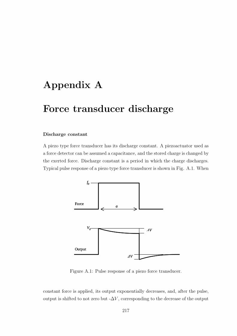
Appendix A
Force transducer discharge
Discharge constant
A piezo type force transducer has its discharge constant. A piezoactuator used as
a force detector can be assumed a capacitance, and the stored charge is changed by
the exerted force. Discharge constant is a period in which the charge discharges.
Typical pulse response of a piezo type force transducer is shown in Fig. A.1. When
Force
Output
∆V
∆V
f0
V0
aForce
Output
∆V
∆V
f0
V0
a
Figure A.1: Pulse response of a piezo force transducer.
constant force is applied, its output exponentially decreases, and, after the pulse,
output is shifted to not zero but -∆V , corresponding to the decrease of the output
217
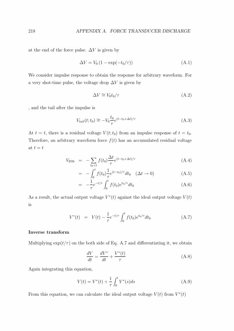
218 APPENDIX A. FORCE TRANSDUCER DISCHARGE
at the end of the force pulse. ∆V is given by
∆V = V0 (1 − exp(−t0/τ)) (A.1)
We consider impulse response to obtain the response for arbitrary waveform. For
a very shot-time pulse, the voltage drop ∆V is given by
∆V ∼= V0t0/τ (A.2)
, and the tail after the impulse is
Vtail(t; t0) ∼= −V0t0τ
e(t−t0+∆t)/τ (A.3)
At t = t, there is a residual voltage V (t; t0) from an impulse response of t = t0.
Therefore, an arbitrary waveform force f(t) has an accumulated residual voltage
at t = t
Vres = −∑t0<t
f(t0)∆t
τe(t−t0+∆t)/τ (A.4)
= −∫ t
0f(t0)
1
τe(t−t0)/τdt0 (∆t → 0) (A.5)
= −1
τe−t/τ
∫ t
0f(t0)e
t0/τdt0 (A.6)
As a result, the actual output voltage V ∗(t) against the ideal output voltage V (t)
is
V ∗(t) = V (t) − 1
τe−t/τ
∫ t
0f(t0)e
t0/τdt0 (A.7)
Inverse transform
Multiplying exp(t/τ ) on the both side of Eq. A.7 and differentiating it, we obtain
dV
dt=
dV ∗
dt+
V ∗(t)τ
(A.8)
Again integrating this equation,
V (t) = V ∗(t) +1
τ
∫ t
0V ∗(s)ds (A.9)
From this equation, we can calculate the ideal output voltage V (t) from V ∗(t)
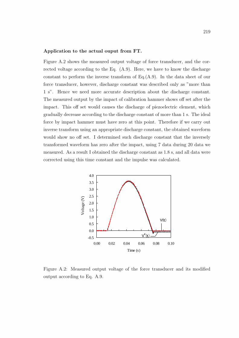
219
Application to the actual ouput from FT.
Figure A.2 shows the measured output voltage of force transducer, and the cor-
rected voltage according to the Eq. (A.9). Here, we have to know the discharge
constant to perform the inverse transform of Eq.(A.9). In the data sheet of our
force transducer, however, discharge constant was described only as ”more than
1 s”. Hence we need more accurate description about the discharge constant.
The measured output by the impact of calibration hammer shows off set after the
impact. This off set would causes the discharge of piezoelectric element, which
gradually decrease according to the discharge constant of more than 1 s. The ideal
force by impact hammer must have zero at this point. Therefore if we carry out
inverse transform using an appropriate discharge constant, the obtained waveform
would show no off set. I determined such discharge constant that the inversely
transformed waveform has zero after the impact, using 7 data during 20 data we
measured. As a result I obtained the discharge constant as 1.8 s, and all data were
corrected using this time constant and the impulse was calculated.
-0.5
0.0
0.5
1.0
1.5
2.0
2.5
3.0
3.5
4.0
0.00 0.02 0.04 0.06 0.08 0.10
Time (s)
Vol
tage
(V)
V(t)
V*
(t)
Figure A.2: Measured output voltage of the force transducer and its modified
output according to Eq. A.9.

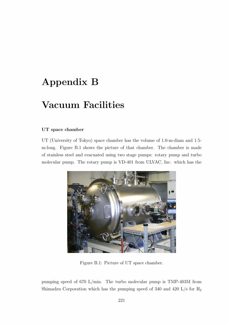
Appendix B
Vacuum Facilities
UT space chamber
UT (University of Tokyo) space chamber has the volume of 1.0-m-diam and 1.5-
m-long. Figure B.1 shows the picture of that chamber. The chamber is made
of stainless steel and evacuated using two stage pumps: rotary pump and turbo
molecular pump. The rotary pump is VD-401 from ULVAC, Inc. which has the
Figure B.1: Picture of UT space chamber.
pumping speed of 670 L/min. The turbo molecular pump is TMP-403M from
Shimadzu Corporation which has the pumping speed of 340 and 420 L/s for H2
221
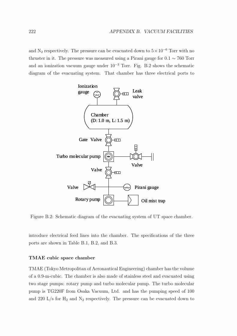
222 APPENDIX B. VACUUM FACILITIES
and N2 respectively. The pressure can be evacuated down to 5×10⁻⁶ Torr with no
thruster in it. The pressure was measured using a Pirani gauge for 0.1 ∼ 760 Torr
and an ionization vacuum gauge under 10−3 Torr. Fig. B.2 shows the schematic
diagram of the evacuating system. That chamber has three electrical ports to
Turbo molecular pump
Valve Pirani gauge
Rotary pump Oil mist trap
Valve
Gate Valve
Valve
Ionization gauge Leak
valve
Chamber(D: 1.0 m, L: 1.5 m)
Turbo molecular pump
Valve Pirani gauge
Rotary pump Oil mist trap
Valve
Gate Valve
Valve
Ionization gauge Leak
valve
Chamber(D: 1.0 m, L: 1.5 m)
Figure B.2: Schematic diagram of the evacuating system of UT space chamber.
introduce electrical feed lines into the chamber. The specifications of the three
ports are shown in Table B.1, B.2, and B.3.
TMAE cubic space chamber
TMAE (Tokyo Metropolitan of Aeronautical Engineering) chamber has the volume
of a 0.9-m-cubic. The chamber is also made of stainless steel and evacuated using
two stage pumps: rotary pump and turbo molecular pump. The turbo molecular
pump is TG220F from Osaka Vacuum, Ltd. and has the pumping speed of 100
and 220 L/s for H2 and N2 respectively. The pressure can be evacuated down to
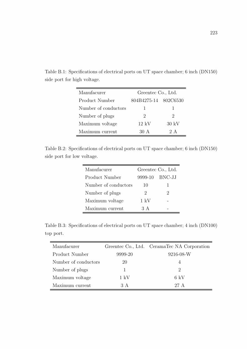
223
Table B.1: Specifications of electrical ports on UT space chamber; 6 inch (DN150)
side port for high voltage.
Manufacurer Greentec Co., Ltd.
Product Number 804B4275-14 802C6530
Number of conductors 1 1
Number of plugs 2 2
Maximum voltage 12 kV 30 kV
Maximum current 30 A 2 A
Table B.2: Specifications of electrical ports on UT space chamber; 6 inch (DN150)
side port for low voltage.
Manufacurer Greentec Co., Ltd.
Product Number 9999-10 BNC-JJ
Number of conductors 10 1
Number of plugs 2 2
Maximum voltage 1 kV -
Maximum current 3 A -
Table B.3: Specifications of electrical ports on UT space chamber; 4 inch (DN100)
top port.
Manufacurer Greentec Co., Ltd. CeramaTec NA Corporation
Product Number 9999-20 9216-08-W
Number of conductors 20 4
Number of plugs 1 2
Maximum voltage 1 kV 6 kV
Maximum current 3 A 27 A
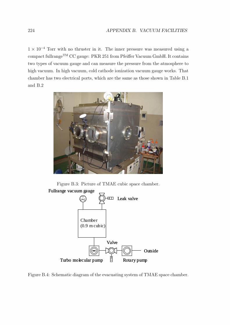
224 APPENDIX B. VACUUM FACILITIES
1 × 10⁻⁴ Torr with no thruster in it. The inner pressure was measured using a
compact fullrangeTM CC gauge: PKR 251 from Pfeiffer Vacuum GmbH. It contains
two types of vacuum gauge and can measure the pressure from the atmosphere to
high vacuum. In high vacuum, cold cathode ionization vacuum gauge works. That
chamber has two electrical ports, which are the same as those shown in Table B.1
and B.2
Figure B.3: Picture of TMAE cubic space chamber.
Turbo molecular pump Rotary pump
Outside
Valve
Fullrange vacuum gauge
Leak valve
Chamber(0.9 m cubic)
Turbo molecular pump Rotary pump
Outside
Valve
Fullrange vacuum gauge
Leak valve
Chamber(0.9 m cubic)
Figure B.4: Schematic diagram of the evacuating system of TMAE space chamber.

Appendix C
Amplitudes of Random Process
Noise
Amplitudes of periodic random process noise is related to the power spectrum and
corelation function. Arbitrary function x(t) with a finite period of (−l/2, l/2) can
be expressed using the Fourier serie
x(t) =∞∑
n=1
(an cosωnt + bn sinωnt) , ωn =2nπ
l(C.1)
⎧⎪⎪⎪⎪⎪⎪⎨⎪⎪⎪⎪⎪⎪⎩
an =2
l
∫ 2/l
−2/lx(t) cosωntdt
bn =2
l
∫ 2/l
−2/lx(t) sinωntdt
(C.2)
Here we will obtaine the ensembel average of the squared amplitude, A2n.
A2n = a2
n + b2n
=4
l2
∫ 2/l
−2/ldt∫ 2/l
−2/ldt′[x(t)x(t′) cosωnt cos ωnt
′ + sinωnt sinωnt′]
=4
l2
∫ 2/l
−2/ldt∫ 2/l
−2/ldt′[x(t)x(t′) cos ωn(t − t′)
], (C.3)
and
< A2n > =
4
l2
∫ 2/l
−2/ldt∫ 2/l
−2/ldt′[
< x(t)x(t′) > cos ωn(t − t′)]
=4
l2
∫ 2/l
−2/ldt∫ 2/l−t
−2/l−tdτ[R(τ ) cos ωnτ
]
225
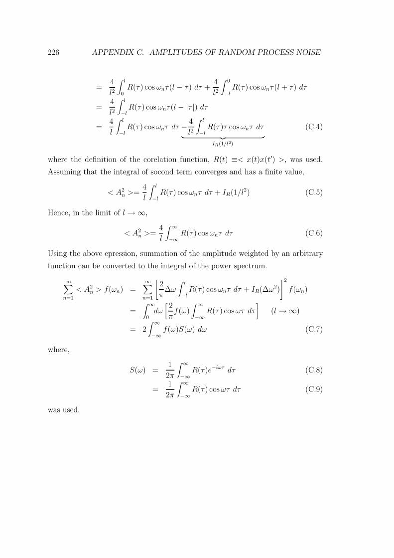
226 APPENDIX C. AMPLITUDES OF RANDOM PROCESS NOISE
=4
l2
∫ l
0R(τ ) cos ωnτ (l − τ ) dτ +
4
l2
∫ 0
−lR(τ ) cos ωnτ (l + τ ) dτ
=4
l2
∫ l
−lR(τ ) cos ωnτ (l − |τ |) dτ
=4
l
∫ l
−lR(τ ) cos ωnτ dτ − 4
l2
∫ l
−lR(τ )τ cos ωnτ dτ︸ ︷︷ ︸
IR(1/l2)
(C.4)
where the definition of the corelation function, R(t) ≡< x(t)x(t′) >, was used.
Assuming that the integral of socond term converges and has a finite value,
< A2n >=
4
l
∫ l
−lR(τ ) cos ωnτ dτ + IR(1/l2) (C.5)
Hence, in the limit of l → ∞,
< A2n >=
4
l
∫ ∞
−∞R(τ ) cos ωnτ dτ (C.6)
Using the above epression, summation of the amplitude weighted by an arbitrary
function can be converted to the integral of the power spectrum.
∞∑n=1
< A2n > f(ωn) =
∞∑n=1
[2
π∆ω
∫ l
−lR(τ ) cos ωnτ dτ + IR(∆ω2)
]2
f(ωn)
=∫ ∞
0dω[2
πf(ω)
∫ ∞
−∞R(τ ) cos ωτ dτ
](l → ∞)
= 2∫ ∞
−∞f(ω)S(ω) dω (C.7)
where,
S(ω) =1
2π
∫ ∞
−∞R(τ )e−iωτ dτ (C.8)
=1
2π
∫ ∞
−∞R(τ ) cos ωτ dτ (C.9)
was used.
Appendix D
Thermal Conductivity of Mixture
Solid
Predictions of the thermal conductivity of heterogeneous solid mixture have been
developed by several authors [87, 88, 89, 90, 91]. To date, however, no general
equation exisits to predict it. The thermal conductivity of heterogeneous solid
mixture depends on the phase geometry as well as the on the properties of mate-
rials. Here, several predictions are summerized.
Nomenclature
p: volume fraction of mixed solid
kc: thermal conductivity of continuous phase
kd: thermal conductivity of discontinuous phase
km: thermal conductivity of mixed phase
λ : ratio of thermal conductivities of discontinuous phase (kd/kc)
λm : ratio of thermal conductivities of mixed solid(km/kc)
Maxwell
λm =λ + 2 − 2p(1 − λ)
λ + 2 + p(1 − λ)(D.1)
which is derived from the electrostatic field problem on the dielectric with porus
(p 1).
Kobayashi et. al [87] conducted the numerical analysis in heterogeneous solid
mixture with the voronoi-polyhedron element method, and derived the following
227
228 APPENDIX D. THERMAL CONDUCTIVITY OF MIXTURE SOLID
empirical equation
λm =C1λ1 + C2λ2 + C3λ3
C1 + C2 + C3(D.2)
F = ln
(λ + 1/λ
2
), G = 5(1 − 2p)((1 − p)p)0.75 ln λ + 1
λ1 =λ
(1 − p)λ + p, C1 = Fp1.1
λ2 = pλ0.75 + (1 − p)1.25 , C2 = 0.9F (1 − p)1.5
λ3 = λp , C3 = pλ(2−3p)/2
Woodside [90]
λm =
(a1 − 1
2aln(
a + 1
a − 1
)− 1
)R + 1
−1
(D.3)
R =(
6p
π
)1/3
, a =
√4
π(λ − 1)R2+ 1
Russel [91]
λm =λp2/3 + (1 − p2/3)
λ(p2/3 − p) + (1 − p2/3 + p)(D.4)
Yuge [88]
λm =dx +
√d2
x + 8d1d2
4(D.5)
d1 = (1 − p) + pd0d0 =2λ
λ + 1d2 = pλ + (1 − p)d0 , dx = (2 − 3p)d1 + (3p− 1)d2
Cheng and Vachon [89]
λm =
1
αβln
(2α + βB
2α − βB
)+ 1 − B
−1
(D.6)
B =√
3p/2 ,
α =√
(λ − 1)B + 1 , β =√
4|λ − 1| + B
Boron potassium nitrate that is a pyrotechnic used in this study is mixture of
boron in potassium nitrate. The thermal conductivity of boron is listed in Table
D.1. It largely depdends on the temperature from 27.6 to 6.29 W/mK correspoindg
temperature of 300 to 1000 K. On the other hand, the thermal conductivity of
229
molten potassium nitrate remained around 0.4 ∼ 0.5 W/mK [121]. The diameter
of the mixed boron particle was less than 1.0 µm and the weight fraction of 0.30
and the volume fractionof 0.27. Due to its large difference of the conductivities
and not small volume fraction, the accurate prediciton of the B/KNO3 pellet is
difficult.
Table D.1: Thermal conductivity of boron.
Temperature (K) Thermal conductivity (W/mK)
300 27.6
400 18.7
700 9.41
1000 6.29
5
4
3
2
1
0Rat
io o
f th
erm
al c
ondu
ctiv
ities
of
mix
ture
1100900700500300
Temperature (K)
Kobayashi Woodside Maxwell Russell Yuge Cheng
Vorume fraction of boron: 0.272
Figure D.1: Thermal conductivity of boron-mixed-KNO3, temperature depen-
dence
230 APPENDIX D. THERMAL CONDUCTIVITY OF MIXTURE SOLID
5.0
4.0
3.0
2.0
1.0
0.0Rat
io o
f th
erm
al c
ondu
ctiv
ities
of
mix
ture
0.500.400.300.200.100.00
Volume fraction of boron particle
Kobayashi Woodside Maxwell Russell Yuge Cheng
kB = 18.7 W/mK at 400 KkKNO3 = 0.45 W/mK
Figure D.2: Thermal conductivity of boron-mixed-KNO3, dependence on the vol-
ume fraction of boron at 400 K.
5.0
4.0
3.0
2.0
1.0
0.0Rat
io o
f th
erm
al c
ondu
ctiv
ities
of
mix
ture
0.50.40.30.20.10.0
Volume fraction of boron particle
kB = 9.4 W/mK at 700 KkKNO3 = 0.45 W/mK
Kobayashi Woodside Maxwell Russell Yuge Cheng
Figure D.3: Thermal conductivity of boron-mixed-KNO3, dependence on the vol-
ume fraction of boron at 700 K.
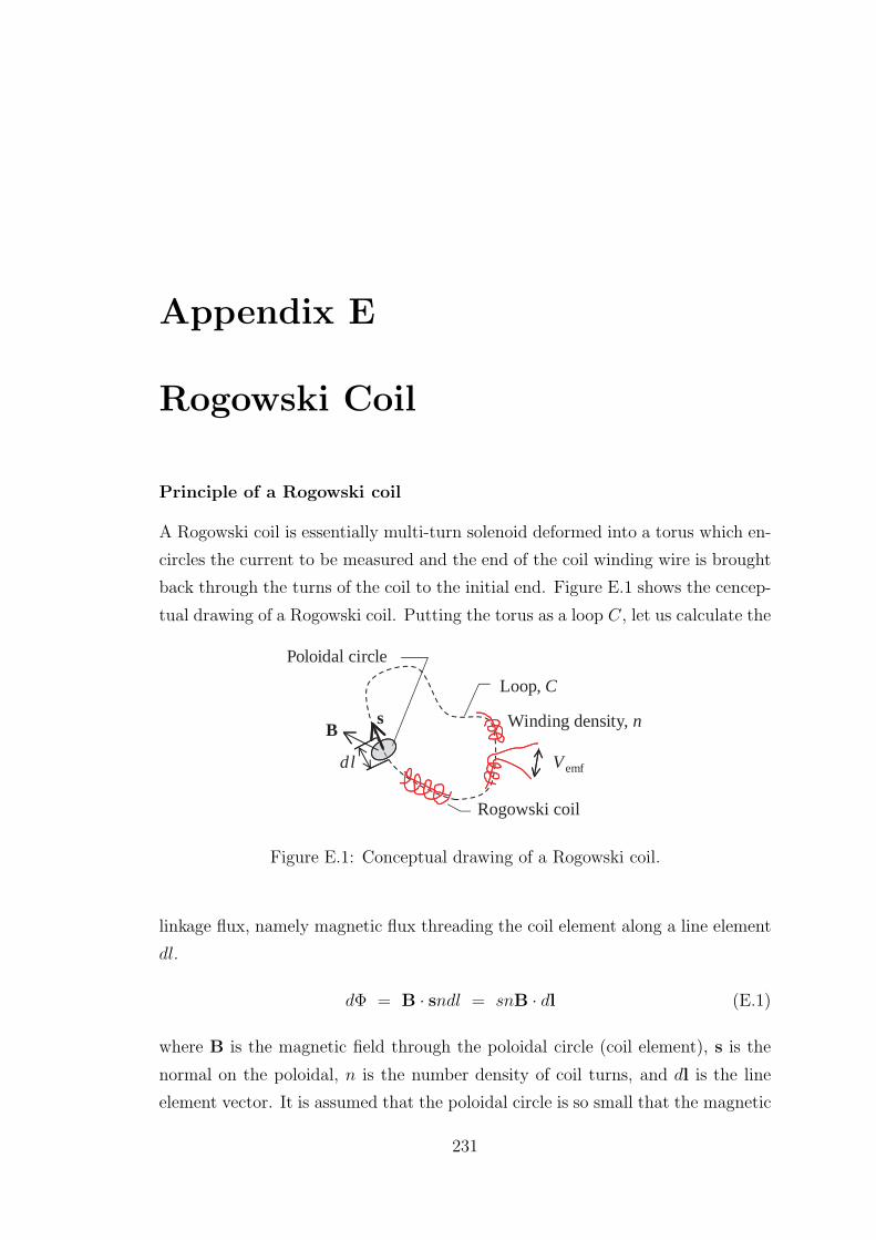
Appendix E
Rogowski Coil
Principle of a Rogowski coil
A Rogowski coil is essentially multi-turn solenoid deformed into a torus which en-
circles the current to be measured and the end of the coil winding wire is brought
back through the turns of the coil to the initial end. Figure E.1 shows the cencep-
tual drawing of a Rogowski coil. Putting the torus as a loop C , let us calculate the
dl
Loop, C
sB Winding density, n
Poloidal circle
V emf
Rogowski coil
Figure E.1: Conceptual drawing of a Rogowski coil.
linkage flux, namely magnetic flux threading the coil element along a line element
dl.
dΦ = B · sndl = snB · dl (E.1)
where B is the magnetic field through the poloidal circle (coil element), s is the
normal on the poloidal, n is the number density of coil turns, and dl is the line
element vector. It is assumed that the poloidal circle is so small that the magnetic
231
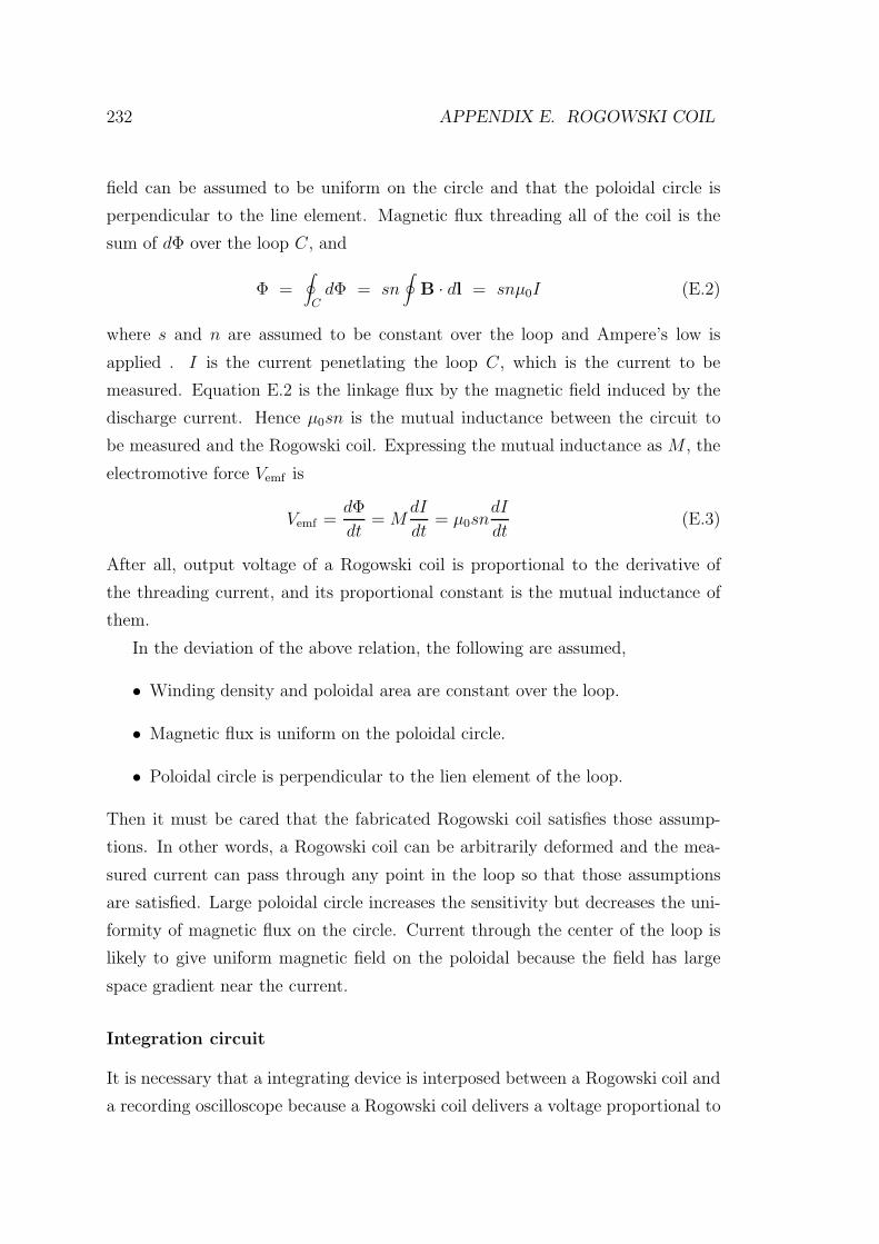
232 APPENDIX E. ROGOWSKI COIL
field can be assumed to be uniform on the circle and that the poloidal circle is
perpendicular to the line element. Magnetic flux threading all of the coil is the
sum of dΦ over the loop C , and
Φ =∮
CdΦ = sn
∮B · dl = snµ0I (E.2)
where s and n are assumed to be constant over the loop and Ampere’s low is
applied . I is the current penetlating the loop C , which is the current to be
measured. Equation E.2 is the linkage flux by the magnetic field induced by the
discharge current. Hence µ0sn is the mutual inductance between the circuit to
be measured and the Rogowski coil. Expressing the mutual inductance as M , the
electromotive force Vemf is
Vemf =dΦ
dt= M
dI
dt= µ0sn
dI
dt(E.3)
After all, output voltage of a Rogowski coil is proportional to the derivative of
the threading current, and its proportional constant is the mutual inductance of
them.
In the deviation of the above relation, the following are assumed,
• Winding density and poloidal area are constant over the loop.
• Magnetic flux is uniform on the poloidal circle.
• Poloidal circle is perpendicular to the lien element of the loop.
Then it must be cared that the fabricated Rogowski coil satisfies those assump-
tions. In other words, a Rogowski coil can be arbitrarily deformed and the mea-
sured current can pass through any point in the loop so that those assumptions
are satisfied. Large poloidal circle increases the sensitivity but decreases the uni-
formity of magnetic flux on the circle. Current through the center of the loop is
likely to give uniform magnetic field on the poloidal because the field has large
space gradient near the current.
Integration circuit
It is necessary that a integrating device is interposed between a Rogowski coil and
a recording oscilloscope because a Rogowski coil delivers a voltage proportional to
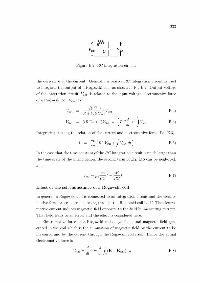
233
Vemf VoutC
RVemf VoutC
R
Figure E.2: RC integration circuit.
the derivative of the current. Generally a passive RC integration circuit is used
to integrate the output of a Rogowski coil, as shown in Fig.E.2. Output voltage
of the integration circuit, Vout, is related to the input voltage, electromotive force
of a Rogowski coil Vemf as
Vout =1/(iCω)
R + 1/(iCω)Vemf (E.4)
Vemf = (iRCω + 1)Vout =
(RC
d
dt+ 1
)Vout (E.5)
Integrating it using the relation of the current and electromotive force, Eq. E.3,
I =µ0
sn
(RCVout +
∫Vout dt
)(E.6)
In the case that the time constant of the RC integration circuit is much larger than
the time scale of the phenomenon, the second term of Eq. E.6 can be neglected,
and
Vout = µ0sn
RCI =
M
RCI (E.7)
Effect of the self inductance of a Rogowski coil
In general, a Rogowski coil is connected to an integration circuit and the electro-
motive force causes current passing through the Rogowski coil itself. The electro-
motive current induces magnetic field opposite to the field by measuring current.
That field leads to an error, and the effect is considered here.
Electromotive force on a Rogowski coil obeys the actual magnetic field gen-
erated in the coil which is the summation of magnetic field by the current to be
measured and by the current through the Rogowski coil itself. Hence the actual
electromotive force is
Vemf =d
dtΦ =
d
dt
∮C(B − Bemf) · dl (E.8)
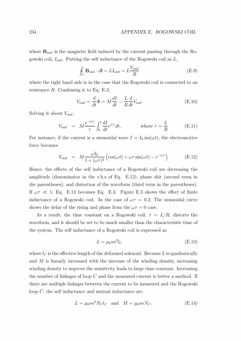
234 APPENDIX E. ROGOWSKI COIL
where Bemf is the magnetic field induced by the current passing through the Ro-
gowski coil, Iemf . Putting the self inductance of the Rogowski coil as L,∮CBemf · dl = LIemf = L
Vemf
R(E.9)
where the right hand side is in the case that the Rogowski coil is connected to an
resistance R. Combining it to Eq. E.3,
Vemf =d
dtΦ = M
dI
dt− L
R
d
dtVemf (E.10)
Solving it about Vemf ,
Vemf = Me−t/τ
τ
∫ t
0
dI
dtet/τdt, where τ =
L
R(E.11)
For instance, if the current is a sinusoidal wave I = I0 sin(ωt), the electromotive
force becomes
Vemf = MωI0
1 + (ωτ)2
(cos(ωt) + ωτ sin(ωt) − e−t/τ
)(E.12)
Hence, the effects of the self inductance of a Rogowski coil are decreasing the
amplitude (denominator in the r.h.s of Eq. E.12), phase shit (second term in
the parentheses), and distortion of the waveform (third term in the parentheses).
If ωτ 1, Eq. E.12 becomes Eq. E.3. Figure E.3 shows the effect of finite
inductance of a Rogowski coil. In the case of ωτ = 0.2, The sinusoidal curve
shows the delay of the rising and phase from the ωτ = 0 case.
As a result, the time constant on a Rogowski coil, τ = L/R, distorts the
waveform, and it should be set to be much smaller than the characteristic time of
the system. The self inductance of a Rogowski coil is expressed as
L = µ0sn2lC (E.13)
where lC is the effective length of the deformed solenoid. Because L is quadratically
and M is linearly increased with the inrcease of the winding density, increasing
winding density to improve the sensitivity leads to large time constant. Increasing
the number of linkages of loop C and the measured current is better a method. If
there are multiple linkages between the current to be measured and the Rogowski
loop C , the self inductance and mutual inductance are
L = µ0sn2NClC and M = µ0snNC . (E.14)
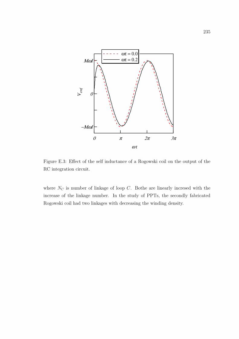
235
−ΜωΙ
0
ΜωΙ
Vem
f
0 π 2π 3π
ω t
ωτ = 0.0 ωτ = 0.2
Figure E.3: Effect of the self inductance of a Rogowski coil on the output of the
RC integration circuit.
where NC is number of linkage of loop C . Bothe are linearly incresed with the
increase of the linkage number. In the study of PPTs, the secondly fabricated
Rogowski coil had two linkages with decreasing the winding density.


Appendix F
Electrical Circuit Diagrams
237
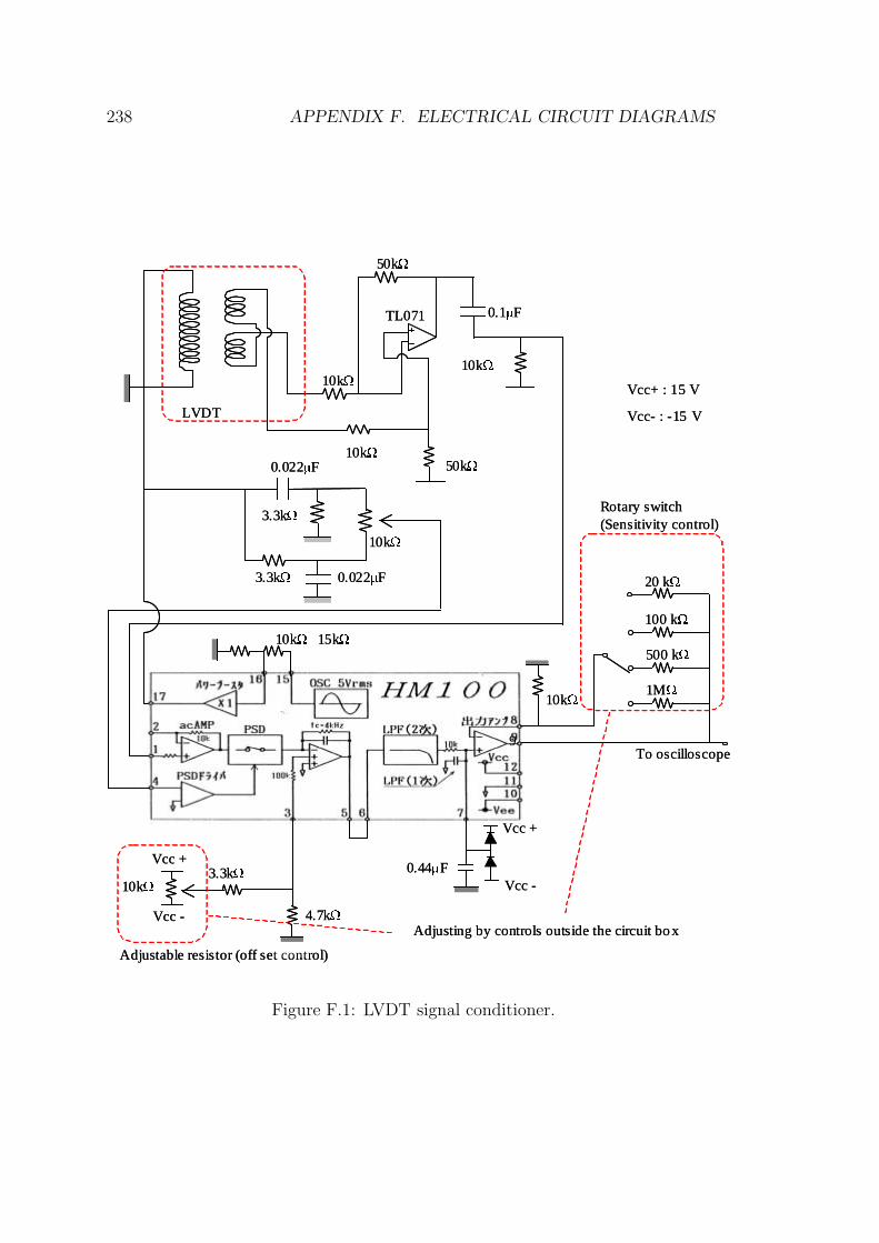
238 APPENDIX F. ELECTRICAL CIRCUIT DIAGRAMS
Vcc+ : 15 V
Vcc- : -15 V
TL071
10kΩ 15kΩ
10kΩ
20 kΩ
Vcc +
Vcc -
10kΩ3.3kΩ
4.7kΩ
9
10kΩ
3.3kΩ
3.3kΩ
10kΩ50kΩ
0.022µF
0.022µF
10kΩ10kΩ
0.1µF
50kΩ
0.44µF
Vcc +
Vcc -
LVDT
To oscilloscope
100 kΩ
500 kΩ
1MΩ
Rotary switch(Sensitivity control)
Adjustable resistor (off set control)
Adjusting by controls outside the circuit bo x
Figure F.1: LVDT signal conditioner.
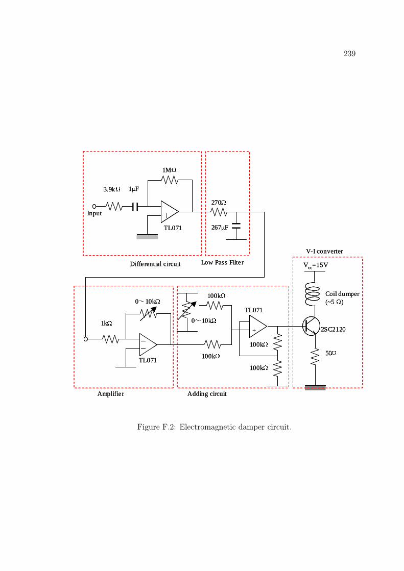
239
0~10kΩ
-
+
3.9kΩ
1MΩ
270Ω
1kΩ
0~10kΩ100kΩ
100kΩ
100kΩ
100kΩ
Vcc=15V
TL071
TL071
50Ω
Coil dumper(~5 Ω)
1µF
267µF
2SC2120
TL071
Differential circuit Low Pass Filter
Input-
+
-
+
Amplifier Adding circuit
V-I converter
0~10kΩ
-
+
3.9kΩ
1MΩ
270Ω
1kΩ
0~10kΩ100kΩ
100kΩ
100kΩ
100kΩ
Vcc=15V
TL071
TL071
50Ω
Coil dumper(~5 Ω)
1µF
267µF
2SC2120
TL071
Differential circuit Low Pass Filter
Input-
+
-
+-
+
Amplifier Adding circuit
V-I converter
Figure F.2: Electromagnetic damper circuit.
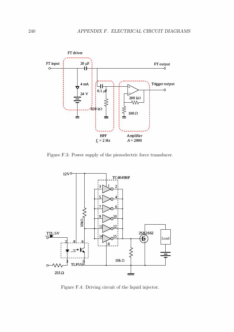
240 APPENDIX F. ELECTRICAL CIRCUIT DIAGRAMS
FT driver
HPFfc = 2 Hz
AmplifierA = 2000
4 mA
24 V0.1 µF
20 µF
820 kΩ100 Ω
200 kΩ
FT input FT output
Trigger output
FT driver
HPFfc = 2 Hz
AmplifierA = 2000
4 mA
24 V0.1 µF
20 µF
820 kΩ100 Ω
200 kΩ
FT input FT output
Trigger output
Figure F.3: Power supply of the piezoelectric force transducer.
TC4049BP
2
3 5
6
TLP550
255 Ω
10kΩ
10k Ω
1 23
45
67
109
1211
1514
8
12V
2SK2662Load
TTL:5V
8
TC4049BP
2
3 5
6
TLP550
255 Ω
10kΩ
10k Ω
1 23
45
67
109
1211
1514
8
12V
2SK2662Load
TTL:5V
8
Figure F.4: Driving circuit of the liquid injector.
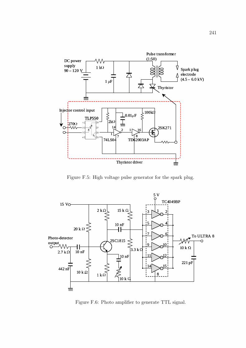
241
Thyristor
1 kΩ
1 µF
Pulse transformer (1:50)DC power
supply90 – 120 V Spark p lug
electrode(4.5 – 6.0 kV)
TLP5502kΩ
0.01µF100kΩ
270Ω2SK271
17
142 1
8
16
74LS04 TD62003AP
Thyristor driver
Injector control input
Thyristor
1 kΩ
1 µF
Pulse transformer (1:50)DC power
supply90 – 120 V Spark p lug
electrode(4.5 – 6.0 kV)
TLP550TLP5502kΩ
0.01µF100kΩ
270Ω2SK271
17
142 1
8
16
74LS04 TD62003AP
Thyristor driver
Injector control input
Figure F.5: High voltage pulse generator for the spark plug.
TC4049BP
1 23
45
67
109
1211
1514
8
5 V
15 V
Photo-detector output
To ULTRA 8
10 k Ω
221 pF
10 nF
10 nF
10 nF
442 nF
2.7 k Ω
20 k Ω
2 k Ω 15 k Ω
3.3 k Ω
10 k Ω1 k Ω
10 k Ω
2SC1815
TC4049BP
1 23
45
67
109
1211
1514
8
5 V
15 V
Photo-detector output
To ULTRA 8
10 k Ω
221 pF
10 nF
10 nF
10 nF
442 nF
2.7 k Ω
20 k Ω
2 k Ω 15 k Ω
3.3 k Ω
10 k Ω1 k Ω
10 k Ω
2SC1815
Figure F.6: Photo amplifier to generate TTL signal.
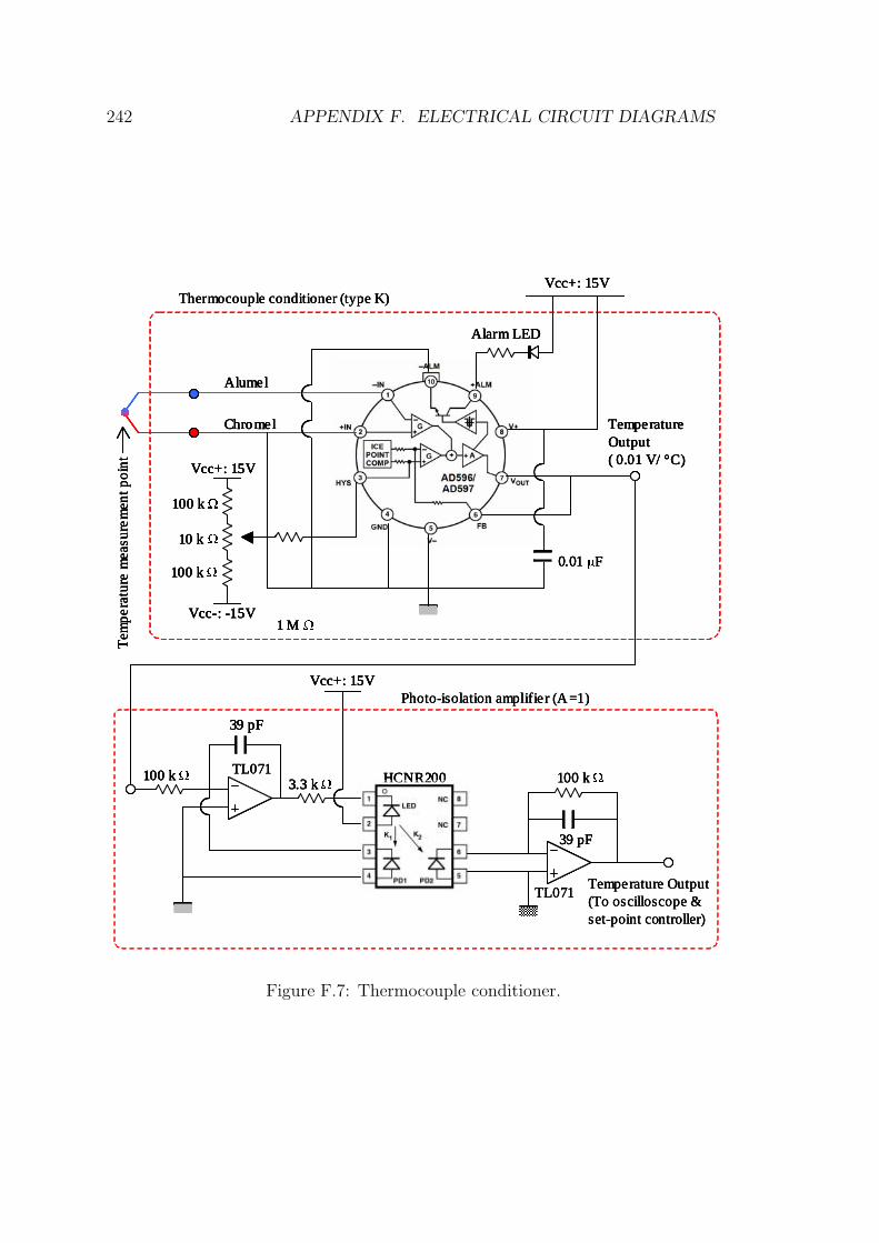
242 APPENDIX F. ELECTRICAL CIRCUIT DIAGRAMS
TL071
TL071
0.01 µF
Vcc+: 15V
Vcc-: -15V
Vcc+: 15V
Alumel
Chromel Temperature Output( 0.01 V/ °C)
100 k Ω
100 k Ω
10 k Ω
1 M Ω
Alarm LED
Vcc+: 15V
3.3 k Ω100 k Ω 100 k Ω
39 pF
39 pF
HCNR200
Thermocouple conditioner (type K)
Photo-isolation amplifier (A =1)
Tem
pera
ture
mea
sure
men
t poi
nt
Temperature Output(To oscilloscope &set-point controller)
TL071
TL071
0.01 µF
Vcc+: 15V
Vcc-: -15V
Vcc+: 15V
Alumel
Chromel Temperature Output( 0.01 V/ °C)
100 k Ω
100 k Ω
10 k Ω
1 M Ω
Alarm LED
0.01 µF
Vcc+: 15V
Vcc-: -15V
Vcc+: 15V
Alumel
Chromel Temperature Output( 0.01 V/ °C)
100 k Ω
100 k Ω
10 k Ω
1 M Ω
Alarm LED
Vcc+: 15V
3.3 k Ω100 k Ω 100 k Ω
39 pF
39 pF
HCNR200
Vcc+: 15V
3.3 k Ω100 k Ω 100 k Ω
39 pF
39 pF
HCNR200
Thermocouple conditioner (type K)
Photo-isolation amplifier (A =1)
Tem
pera
ture
mea
sure
men
t poi
nt
Temperature Output(To oscilloscope &set-point controller)
Figure F.7: Thermocouple conditioner.
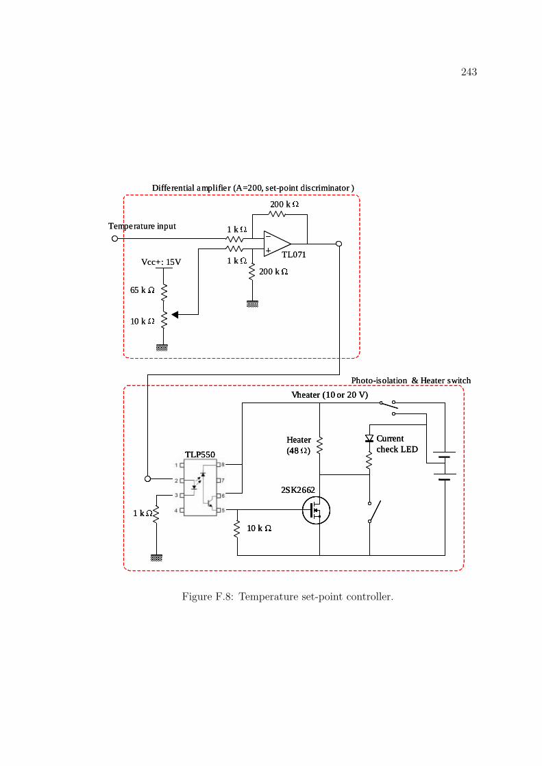
243
Vheater (10 or 20 V)
TLP550
2SK2662
1 k Ω
10 k Ω
Heater (48 Ω)
Current check LED
200 k Ω
Vcc+: 15V
65 k Ω
10 k Ω
200 k Ω
1 k Ω
1 k ΩTL071
Differential amplifier (A=200, set-point discriminator )
Photo-isolation & Heater switch
Temperature input
Vheater (10 or 20 V)
TLP550
2SK2662
1 k Ω
10 k Ω
Heater (48 Ω)
Current check LED
Vheater (10 or 20 V)
TLP550TLP550
2SK2662
1 k Ω
10 k Ω
Heater (48 Ω)
Current check LED
200 k Ω
Vcc+: 15V
65 k Ω
10 k Ω
200 k Ω
1 k Ω
1 k ΩTL071
Differential amplifier (A=200, set-point discriminator )
Photo-isolation & Heater switch
Temperature input
Figure F.8: Temperature set-point controller.