C H I A N G M A I U N I V E R S I T Y J O U R N A L O F S O C I A L S C I E N C E A N D H U M A N I T I E S

143

CM

U. Journal of Soc. Sci. and H

uman. (2008) Vol. 2(2)

M. N. A. Bhuiyan1*, Kazi Saleh Ahmed2 and Roushan Jahan1

Study on Modeling and Forecasting of the GDPof Manufacturing Industries in Bangladesh

1Department of Mechanical Engineering, Tokyo Metropolitan University, 1-1, Minami-Osawa, Hachioji-shi, Tokyo 192-0397, Japan. 2Department of Statistics, Jahangirnagar University, Savar, Dhaka-1342, Bangladesh. *Corresponding author. E-mail: alam78bh@ed.tmu.ac.jp

ABSTRACT

Forecasting of the GDP of manufacturing industries plays a major role in optimal decision formulae for government and industrial

sector in Bangladesh. This study aimed to divulge the contribution of this sector to the overall GDP for the next thirteen years, beginning from 2002-03, by using an appropriate model. To develop the appropriate model, time series data have been used. Since forecasting is one main objective of building the time series model, therefore at present, time series data are widely and frequently applied in the area of empirical research. Autoregressive Integrated Moving Average (ARIMA) or Box-Jenkins methodology is most popular for forecasting stationary time series data. To make forecast, firstly, we test the stationarity of the data, secondly, develop an appro-priate ARIMA model and finally, make forecast based on the selected model. Based on Autocor-relation Function (ACF), Partial Autocorrelation Function (PACF) and resulting correlogram, the data are seen to be nonstationary. To make the data stationary, we have to take second difference. Primarily, nine ARIMA models are considered for GDP of Manufacturing Industries. After that we select three ARIMA models, i.e., ARIMA (220), ARIMA (221) and ARIMA (222) on the basis of smallest Akaike Information Criteria (AIC) and Bayesian Information Criteria (BIC). Finally, ARIMA (221) is selected from these pre-selected models for GDP of Manufacturing Industries, based on the smallest values of Standard Error (SE (σ)), Absolute Mean Error (AME), Root Mean Square Error (RMSE) and Mean Absolute Percent Error (MAPE) and forecasting is made by using this model. In this paper, we divide the total period into two parts: i) Estimation period and ii) Forecast period. In the estimation period, we see that our estimated value fits the data very well and then we make forecast for the mentioned years. The forecast value of the manufacturing industries GDP shows a sus- tainable upward trend.

CMU. J. of Soc. Sci. and Human. 2008

144

CM

U. Journal of Soc. Sci. and H

uman. (2008) Vol. 2(2)

Key words: Forecasting, ARIMA, Stationary, ACF, PACF, AIC, BIC, SE (σ), AME, RMSE, MAPE.

INTRODUCTION

Manufacturing sector is one of the important activity sectors of a country. In case of Bangladesh, the contribution of this sector to

national production and growth is not at a considerable level. The share of manufacturing industry in overall GDP in Bangladesh ranged from 9.4% in FY 1997-1998 to 15.62% in FY 2001-2002. The sectoral growth of GDP of manufacturing is 5% in 2001-2002. No strong courses of action have yet been taken to improve this sector. It is necessary to make forecast of the GDP of this sector for the future period so that the government and policy makers can set up their plans to get better output. Some of the cited literatures related to forecasting are discussed below: Paul (1998) worked with “Modeling and Forecasting of Energy Consumption in Bangladesh”. He applied Box-Jenkins (BJ) methodo-logy or ARIMA methodology in his study and found that the data were nonstationary. After making the data stationary, he selected three ARIMA models on the basis of smallest AIC and BIC and finally selected the best ARIMA model based on minimum values of AME, RMSE, SE(σ) and MAPE and made forecast by this model. He made forecast by dividing the total period into three parts, namely, estimation period, validation period and forecast period. Helal Uddin (1998) showed the economic and envi-ronmental trend from 1996 to 2003 by using the time series from 1975 to 1995. He examined the stationarity of time series data and found that they were nonstationary. The data were made stationary by transforming them and constructed ARIMA model and forecasting was performed based on the model. Pindyck and Rubinfeld (1976) discussed about the properties of stationary and nonstationary time series, the calculation and the use of autocorrelation function and developed the methods by which time series models were specified, estimated and used for forecasting. They also showed how some non-stationary time series models could be differenced once or many times to produce a stationary series that enabled to develop a general integrated auto regressive moving average (ARIMA) model. By using the data from 1960 to 1967, they forecast the U.S hog production over a two-year horizon, using ARIMA model. Darmodar N. Gujrati (1995) examined the US GDP time series for the quarterly periods of 1970 to 1991. He found that US GDP was nonstationary on the basis of ACF and PACF. After making the first difference, it was stationary. He also applied

C H I A N G M A I U N I V E R S I T Y J O U R N A L O F S O C I A L S C I E N C E A N D H U M A N I T I E S

145

CM

U. Journal of Soc. Sci. and H

uman. (2008) Vol. 2(2)

four-step Box-Jenkins (BJ) or ARIMA methodology: identification, estima-tion, diagnostic checking and forecasting to the US GDP data. Using the above-mentioned data, forecasting was made for the first quarter of 1992. Hurvich and Tsai (1989) realized the problem of autoregressive model selection procedure and proposed one of the leading selection methods, AIC (Akaike, 1973). The minimum AIC criterion produces a selected model which is, hopefully, close to the best possible choice. George et al. (1988) discussed about the three stages: i) identification ii) estimation and iii) diagnostic checking of Box-Jenkins approach to find an ARIMA model for a given set of time series data which adequately represented the data-generating process. For each stage, they illustrated the single steps by analyzing the yearly price of corn in the United States from 1867 to 1948 and then made point forecast on the basis of the selected model. Granger et al. (1995) suggested that model selection procedures were better to use rather than formal hypothesis testing at the time of deciding on model specification. They also examined how well the model could be selected depending upon the minimum values of Akaike Information Criteria (AIC) and Bayesian Information Criteria (BIC). Box and Jenkins (1970) described extensively about an iterative model-building methodology. They explained the process of model identification, model estimation and model diagnostic checking for ARIMA model. They also discussed the properties of ARIMA models and showed how the models were used to forecast the future values of an observed time series. In the present study, twenty-three years GDP data of manufacturing industries have been used. The data are collected from Bangladesh Bureau of Statistics (BBS).

MODEL DISCUSSION

In time series analysis, ARIMA models are flexible and widely used. The time series model can provide short-run forecast for sufficiently large

amount of data on the concerned variables very precisely. The abbreviation ARIMA (p, d, q) stands for Autoregressive-Integrated-Moving-Average with three parameters, p, the order of autoregression, d, the degree of differencing and q, the order of moving average. The ARIMA model, commonly known as Box-Jenkins model, is due to Box and Jenkins’ work for forecasting of a large variety of time series data. The underlying assumption is that the time series to be forecast has been generated by a stochastic process. ARIMA model is the combination of three processes such as (1) Auto-regressive (AR) process, (2) Differencing process, and (3) Moving Average (MA) process. These three processes are based on random dis-

CMU. J. of Soc. Sci. and Human. 2008

146

CM

U. Journal of Soc. Sci. and H

uman. (2008) Vol. 2(2)

turbances that arise in the observation of empirical time series.

Auto-regressive Process The auto-regressive process is defined as a linear combination of cur-rent value with its preceding value(s). The first order auto-regressive process AR (1) defines the current value as linear function of single preceding value. Similarly, the pth order auto-regressive process defines the current value as a linear combination of p preceding values. The autoregressive process is commonly denoted by AR (p), where the number in the parenthesis stands for order. Thus, the pth order auto-regressive process of a random variable yt can be represented as follows: yt= µ +α1yt-1+α2yt-2+α3yt-3+……………+αpyt-p+et

Where µ is the intercept parameter that is related to the mean of the variable, α’s known auto-regressive parameters, and the errors et are assumed to be un-correlated random variables with zero mean, and common variance σ2.

Differencing Process Differencing process is an aid to identify the stationarity level of a time series. Level of stationarity is required for forecasting future value, because forecasting is valid only when underlying time series is stationary. If a time series differenced once to make it stationary, then the original series is said to be Integrated of order 1 and is represented by I (1). Similarly, if the original series differenced twice to make it stationary, the original series is said to be Integrated of order 2, and is represented by I (2). In general, if the time series differenced d times, it is Integrated of order d and represented by I (d). By convention, if d=0, the resulting process represents a stationary time series of order zero and is represented by I (0).

Moving Average Process The third of the three processes of ARIMA modeling techniques is the moving average process. The error-generating process that includes the average of two adjacent random variables is known as moving average (MA) process of order one. Similarly, the error generating process that includes average of three adjacent random variables is known as the moving average process of second order. In general, if the error generating process includes the average of q+1 adjacent random variables, the process is known as moving average (MA) process of qth order. Thus, the general qth order moving average process, denoted by MA (q) of a random

C H I A N G M A I U N I V E R S I T Y J O U R N A L O F S O C I A L S C I E N C E A N D H U M A N I T I E S

147

CM

U. Journal of Soc. Sci. and H

uman. (2008) Vol. 2(2)

variable, can be represented as; yt = µ+et- 1et-1- 2et-2- 3et-3-……………… qet-q

Where µ is the intercept parameter that is related to the mean of the variable, ’s are unknown parameters, and the errors et are assumed to be un-correlated random disturbances with zero mean, and common variance σ2.

Notation of Autoregressive Integrated Moving Average Model The general compact form of ARIMA (p, d, q) process can be re-presented as follows: If the original series yt after appropriate times (say d) of differencing yields a series xt, then zt = (1-L)d yt

Where L is the back shift operator, Lyt = yt-1. For d=1, zt =(1-L) yt= yt – yt-1 =∆yt For d=2, zt = ∆yt – ∆yt-1. The differencing operations used to produce a co-variance stationary time series zt. If yt contains a polynomial trend of order d, then the trend can be removed by the differencing operation (1-L)d. If zt satisfies an ARMA (p, q) process, then a(L) zt = b(L) et where a(L) and b(L) are polynomials in the back shift operator L. The original series yt satisfying an ARIMA (p,d,q) process can be expressed as a(L) (1-L)d yt = b(L) et

In this study, the above format of the equation is used to estimate the underlying parameters. If any constant term occurs in the estimated equation, it is to be placed in the right-hand side as an additional term.

Box- Jenkins Approach The BJ methodology consists of four steps, such as (1) identification (2) estimation (3) diagnostic checking and (4) forecasting. These stages of BJ procedure are summarized schematically in the following chart.

Figure 1. Stages in the Box-Jenkins approach.

CMU. J. of Soc. Sci. and Human. 2008

148

CM

U. Journal of Soc. Sci. and H

uman. (2008) Vol. 2(2)

RESULTS AND DISCUSSION

In this section, we first test the stationarity of the data on the basis of ACF, PACF and correlogram and found that the series is nonstationary.

To make the data stationary, we have to take second difference of the data. Temporarily, nine ARIMA models are taken into consideration, namely, ARIMA (020), ARIMA (021), ARIMA (022), ARIMA (120), ARIMA (121), ARIMA (122), ARIMA (220), ARIMA (221) and ARIMA (222). From these, three models are then considered on the basis of smallest AIC and BIC. Estimation of the three models is performed and one model is finally selected according to the smallest AIC, BIC, SE (σ), AME, RMSE and MAPE and forecasting is made based on it. The analysis is performed by using the computer software packages EXCEL and SPSS.

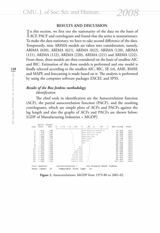
Results of the Box-Jenkins methodology Identification The chief tools in identification are the Autocorrelation function (ACF), the partial autocorrelation function (PACF), and the resulting correlograms, which are simple plots of ACFs and PACFs against the lag length and also the graphs of ACFs and PACFs are shown below: [GDP of Manufacturing Industries = MGDP]

Figure 2. Autocorrelations: MGDP from 1979-80 to 2001-02.

C H I A N G M A I U N I V E R S I T Y J O U R N A L O F S O C I A L S C I E N C E A N D H U M A N I T I E S

149

CM

U. Journal of Soc. Sci. and H

uman. (2008) Vol. 2(2)

Figure 3. Partial Autocorrelations: MGDP from 1979-80 to 2001-02.

Figure 4. ACF of MGDP.

Figure 5. PACF of MGDP.

CMU. J. of Soc. Sci. and Human. 2008

150

CM

U. Journal of Soc. Sci. and H

uman. (2008) Vol. 2(2)

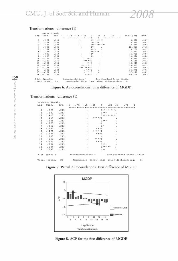
Transformations: difference (1)

Figure 6. Autocorrelations: First difference of MGDP.

Transformations: difference (1)

Figure 7. Partial Autocorrelations: First difference of MGDP.

Figure 8. ACF for the first difference of MGDP.

C H I A N G M A I U N I V E R S I T Y J O U R N A L O F S O C I A L S C I E N C E A N D H U M A N I T I E S

151

CM

U. Journal of Soc. Sci. and H

uman. (2008) Vol. 2(2)

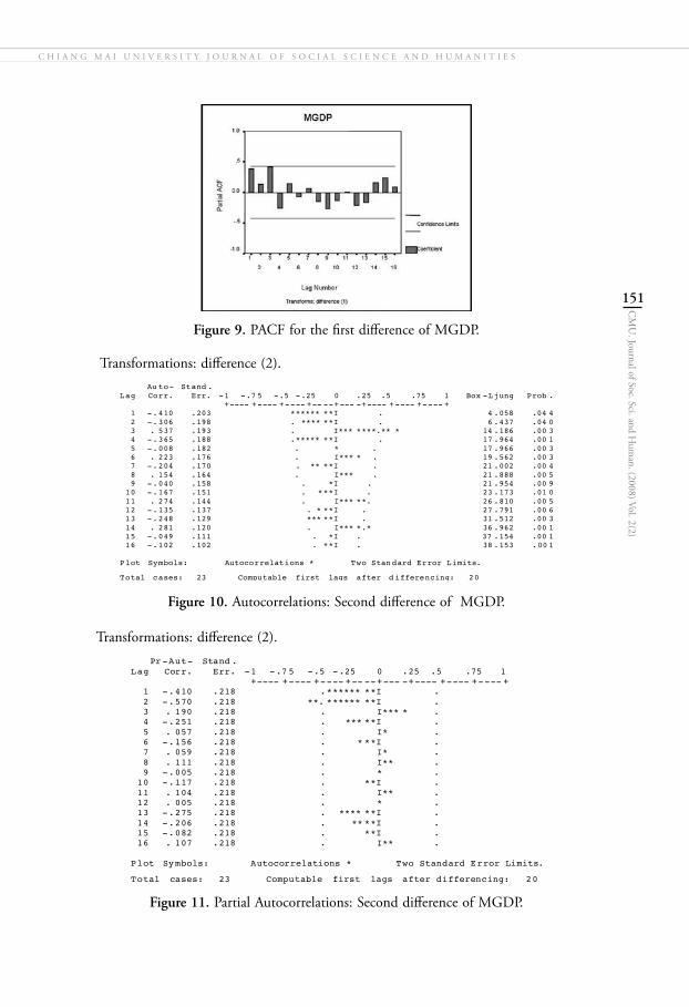
Figure 9. PACF for the first difference of MGDP.

Transformations: difference (2).

Figure 10. Autocorrelations: Second difference of MGDP.

Transformations: difference (2).

Figure 11. Partial Autocorrelations: Second difference of MGDP.

CMU. J. of Soc. Sci. and Human. 2008

152

CM

U. Journal of Soc. Sci. and H

uman. (2008) Vol. 2(2)

Figure 12. ACF for the second difference of MGDP.

Figure 13. PACF for the second difference of MGDP.

Figures 2, 3, 4 and 5 show the correlogram and partial correlogram and the graph of ACF and PACF of the MGDP series. From these figures, two facts stand out: First, the ACF declines very slowly; as shown in figure 2, ACF up to 4 lags out of 16 lags are individually significantly different from zero, for they all are outside the 95% confidence bounds. Second, after the first lag, the PACF drops dramatically, and all PACFs after lag 1 are statistically insignificant. Also, the graph of ACF and PACF shows that the MGDP data do not satisfy the condition of stationarity that are represented in Figure 4 and Figure 5. So the data of Manufacturing GDP is non-stationary. To make the data stationary, we have done some transformation. We did first difference of the data to achieve stationarity. Figures 6, 7, 8 and 9 show the correlogram and partial correlogram and the graph of ACF and PACF of first difference of the data. From these figures, we conclude that the first difference of the data is not stationary.

C H I A N G M A I U N I V E R S I T Y J O U R N A L O F S O C I A L S C I E N C E A N D H U M A N I T I E S

153

CM

U. Journal of Soc. Sci. and H

uman. (2008) Vol. 2(2)

To apply Box –Jenkins methodology, the data must be stationary. For this reason, second difference of the data is made to make it stationary. Figures 10, 11, 12 and 13 show the correlogram and partial correlogram and the graph of ACF and PACF of second difference. This figure shows that the second difference of the MGDP data is stationary. Here, we select primarily nine ARIMA models which have been previously mentioned.

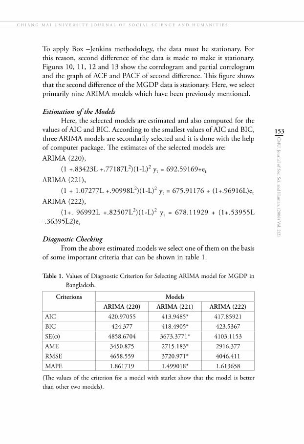
Estimation of the Models Here, the selected models are estimated and also computed for the values of AIC and BIC. According to the smallest values of AIC and BIC, three ARIMA models are secondarily selected and it is done with the help of computer package. The estimates of the selected models are:ARIMA (220), (1 +.83423L +.77187L2)(1-L)2 yt = 692.59169+et

ARIMA (221), (1 + 1.07277L +.90998L2)(1-L)2 yt = 675.91176 + (1+.96916L)et

ARIMA (222), (1+. 96992L +.82507L2)(1-L)2 yt = 678.11929 + (1+.53955L -.36395L2)et

Diagnostic Checking From the above estimated models we select one of them on the basis of some important criteria that can be shown in table 1.

Table 1. Values of Diagnostic Criterion for Selecting ARIMA model for MGDP in Bangladesh.

Criterions Models

ARIMA (220) ARIMA (221) ARIMA (222)

AIC 420.97055 413.9485* 417.85921BIC 424.377 418.4905* 423.5367SE(σ) 4858.6704 3673.3771* 4103.1153AME 3450.875 2715.183* 2916.377RMSE 4658.559 3720.971* 4046.411MAPE 1.861719 1.499018* 1.613658

(The values of the criterion for a model with starlet show that the model is better than other two models).

CMU. J. of Soc. Sci. and Human. 2008

154

CM

U. Journal of Soc. Sci. and H

uman. (2008) Vol. 2(2)

The above table represents that ARIMA (221) shows the minimum values of all criteria comparing to the other two models. So we conclude that ARIMA (221) should be selected to be the best model for forecast-ing.

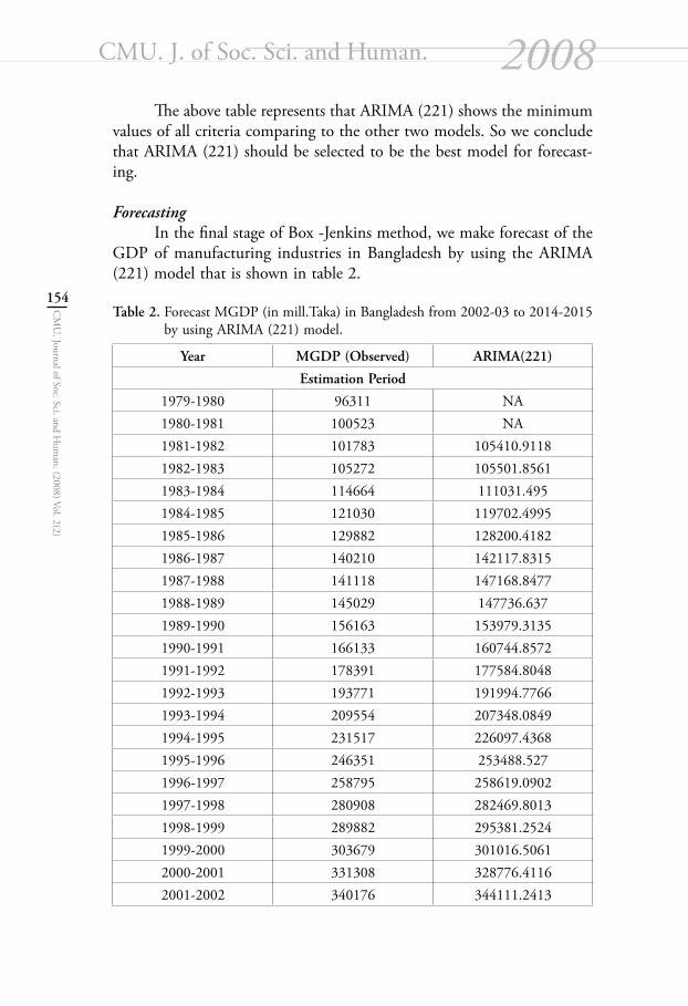
Forecasting In the final stage of Box -Jenkins method, we make forecast of the GDP of manufacturing industries in Bangladesh by using the ARIMA (221) model that is shown in table 2.

Table 2. Forecast MGDP (in mill.Taka) in Bangladesh from 2002-03 to 2014-2015 by using ARIMA (221) model.

Year MGDP (Observed) ARIMA(221)

Estimation Period

1979-1980 96311 NA1980-1981 100523 NA1981-1982 101783 105410.91181982-1983 105272 105501.85611983-1984 114664 111031.4951984-1985 121030 119702.49951985-1986 129882 128200.41821986-1987 140210 142117.83151987-1988 141118 147168.84771988-1989 145029 147736.6371989-1990 156163 153979.31351990-1991 166133 160744.85721991-1992 178391 177584.80481992-1993 193771 191994.77661993-1994 209554 207348.08491994-1995 231517 226097.43681995-1996 246351 253488.5271996-1997 258795 258619.09021997-1998 280908 282469.80131998-1999 289882 295381.25241999-2000 303679 301016.50612000-2001 331308 328776.41162001-2002 340176 344111.2413

C H I A N G M A I U N I V E R S I T Y J O U R N A L O F S O C I A L S C I E N C E A N D H U M A N I T I E S

155

CM

U. Journal of Soc. Sci. and H

uman. (2008) Vol. 2(2)

Forecast Period2002-2003 354882.30682003-2004 382413.672004-2005 392890.06762005-2006 412008.00662006-2007 439391.32742007-2008 452060.26552008-2009 475009.05532009-2010 502335.81892010-2011 517627.65472011-2012 543862.37272012-2013 571325.53792013-2014 589529.13972014-2015 618564.3088

*1 US$= TK. 67 The forecast value of the GDP of manufacturing industries (MGDP) can be shown in the Figure 14.

Figure 14: Forecast GDP in Mill. Tk. of Manaufacturing Industries in Bangladesh from 2002-03 to 2014-15 by using ARIMA (221) model.

In the above figure, MGDP is plotted against their respective years. Here, we showed the previous trend and future trend together. The MGDP shows an upward trend. From the above graph, we see that the past value (data) fits very well, i.e., the estimated line represents the data approximately very closely. From the year 1990-1991, the MGDP shows a linear trend.

CMU. J. of Soc. Sci. and Human. 2008

156

CM

U. Journal of Soc. Sci. and H

uman. (2008) Vol. 2(2)

CONCLUSION

Manufacturing industries are one of the most important economic sectors of a country. In Bangladesh, manufacturing industries are

passing through a tough time. The miserable condition started from during the time of liberation (1971) because most of the industries were out of order at that time. Besides this, political instability is one of the reasons for least development in this sector. Also, due to lower infrastructural development, the local and foreign investors are losing inspiration to invest in this sector. As a result, the development of manufacturing is running at a slow motion. Day by day, the political situation is improving and that’s why the GDP of this sector also shows increasing trend. The result of this paper showed the future picture of manufacturing industries for thirteen years, beginning from 2002-2003. We here would like to quote from the following lines of the Poverty Reduction Strategy Paper (PRSP), the strategy paper for poverty reduction in Bangladesh, “for sustained growth and poverty reduction, the government would pursue a globally-competitive industrialization strategy, dictated by the dynamic comparative advantage of the country. This means an employment-intensive industrialization with emphasis on Small and Medium Enterprises (SMEs) and export-oriented industries”. So it stressed the need of more-strengthened small and medium industrial sector to achieve sustainable economic growth and poverty reduction. Before that, we need concrete evidence of the per-formance of this sector at disaggregated level. This paper discloses the performance of manufacturing sector from 1979-1980 to 2001-2002 and also shows us the future movement. To formulate future development plan for this sector, it is essential to know the previous condition and also see the future trend. In this study, forecasting is done by using some sophisticated statistical tools so that the government and policy makers can easily realize about the future contribution of the GDP of manufac-turing industries to the overall GDP and could take initiatives to how to improve this sector.

REFERENCESBBS, Statistical Year Book of Bangladesh, 1980 to 2000, Bangladesh

Bureau of Statistics (BBS)BBS, National Accounts Statistics of Bangladesh, (Revised Estimates,

1989-90 to 1998-99). BBS, National Accounts Statistics (Gross Domestic Product, 2000-

2001).

C H I A N G M A I U N I V E R S I T Y J O U R N A L O F S O C I A L S C I E N C E A N D H U M A N I T I E S

157

CM

U. Journal of Soc. Sci. and H

uman. (2008) Vol. 2(2)

BBS, National Accounts Statistics (Preliminary Estimates of GDP, 2001-2002).

Box, G.E.P, and Jenkins G.M.1970. TIME SERIES ANALYSIS fore-casting and control. First printing, Holden-Day, Inc., San Francisco, California.

George, G. Judge, R.Carter Hill, William E.Griffiths, Helmut Lutkepohl, and Tsoung-Chaolee. 1988. Introduction to the theory and practice of econometrics. Second Edition, John Wiley & Sons.

Granger, C.W.J., M.L. King, and H. White.1995. Comments on testing economic theories and the use of model selection criteria. Journal of Econometrics, Vol. 67,173-187.

Gujarati, Damodar N.1995. Basic econometrics. Third edition, McGraw-Hill, Inc.

Helal Uddin Ahmed. 1998. Analysis of some selected economic and environmental time series of Bangladesh. PhD Thesis, Department of Statistics, Jahangirnagar University, Dhaka, Bangladesh

Hurvich, Clifford M., and Chih-Ling Tsai.1989. Regression and time series model selection in small samples. Biometrika, Vol. 76, No. 2, 297-307.

Paul, J.C.1998. Modeling and forecasting the energy consumption in Bangladesh. PhD. Thesis, Department of Mathematics, University of North Bengal, West Bengal, India.

Pindyck, R.S., and D.L.R. Rubinfeld. 1976. Econometric models and economic forecasts. McGraw-Hill, New York, Second Edition.

none