Embed Size (px)
Citation preview
Summary notes forEQ2300 Digital Signal Processing
allowed aid for final exams during 2016
Joakim Jalden, 2016-01-12
1 Prerequisites
2 The DFT and the FFT
2.1 The discrete Fourier transform
• The discrete Fourier transform (DTFT) is given by
X(ν) = F{x[n]} ,∞∑
n=−∞x[n]e−j2πνn , ν ∈ R ,
assuming that the integral converges, and it’s inverse is given by
x[n] = F−1{X(ν)} ,∫ 1
0
X(ν)ej2πνndν , n ∈ Z .
• In the above, ν ∈ R is commonly referred to as the normalized frequency.
• Some properties of the DTFT are
– Linearity: x[n]F→ X(ν), y[n]
F→ Y (ν) ⇒ cx[n] + dy[n]F→ cX(ν) + dY (ν)
– Time shift: x[n− k]F→ e−j2πkνX(ν)
– Conjugate symmetry for real valued signals: x[n] ∈ R ⇒ X(ν) = X∗(−ν)
– Parseval’s relation:∞∑
n=−∞
∣∣x[n]∣∣2 =
∫ 1
0
∣∣X(ν)∣∣2dν
• The DTFT X(ν) of a discrete time sequence x[n] is always periodic with period 1, i.e., X(ν+k) = X(ν)for all integers k.
• Examples of the DTFT and more properties are found in the pink collection of formulas.
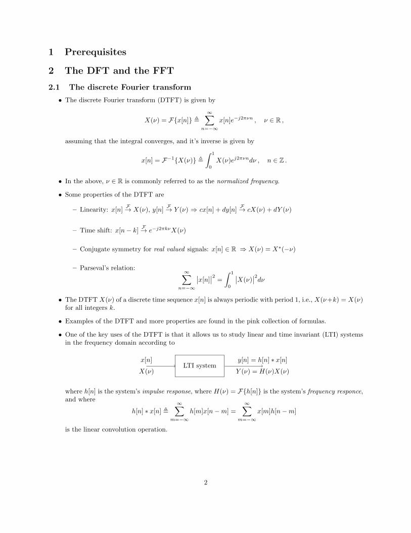
• One of the key uses of the DTFT is that it allows us to study linear and time invariant (LTI) systemsin the frequency domain according to
LTI systemx[n]
X(ν)
y[n] = h[n] ∗ x[n]
Y (ν) = H(ν)X(ν)
where h[n] is the system’s impulse response, where H(ν) = F{h[n]} is the system’s frequency responce,and where
h[n] ∗ x[n] ,∞∑
m=−∞h[m]x[n−m] =
∞∑m=−∞
x[m]h[n−m]
is the linear convolution operation.
2
2.2 The discrete Fourier transform
• The N -point discrete Fourier transform (DFT) is given by
X[k] = FN{x[n]} ,N−1∑n=0
x[n]e−j2πkn/N , k = 0, . . . , N − 1 ,
and it’s inverse is given by
x[n] = F−1N {X[k]} , 1
N
N−1∑k=0
X[k]ej2πkn/N , n = 0, . . . , N − 1 .
• A common alternative notations is
X[k] =
N−1∑n=0
x[n]W knN , where WN , e−j2π/N (the Nth root of unity)
• Some properties of the DFT are
– Linearity: x[n]FN→ X[k], y[n]
FN→ Y [k] ⇒ cx[n] + dy[n]FN→ cX[k] + dY [k]
– Parseval’s relation:∞∑
n=−∞
∣∣x[n]∣∣2 =
1
N
N−1∑k=0
∣∣X[k]∣∣2
– Time shift: x[(n−m) mod N ]FN→ e−j2πkm/NX[k] = W km
N X[k]
– Convolution in time: x[n] N y[n]FN→ X[k]Y [k]
– Multiplication in time: x[n]y[n]FN→ N−1X[k] N Y [k]
where n mod N denotes the modulo N operation (i.e., n mod N is for any n ∈ Z the unique integerin the range 0, . . . , N − 1 of the from n − Nk where k ∈ Z), and N denotes the N -point circularconvolution defined by
x[n] N y[n] ,N−1∑m=0
x[m]y[(n−m) mod N ] =
N−1∑m=0
y[m]x[(n−m) mod N ] .
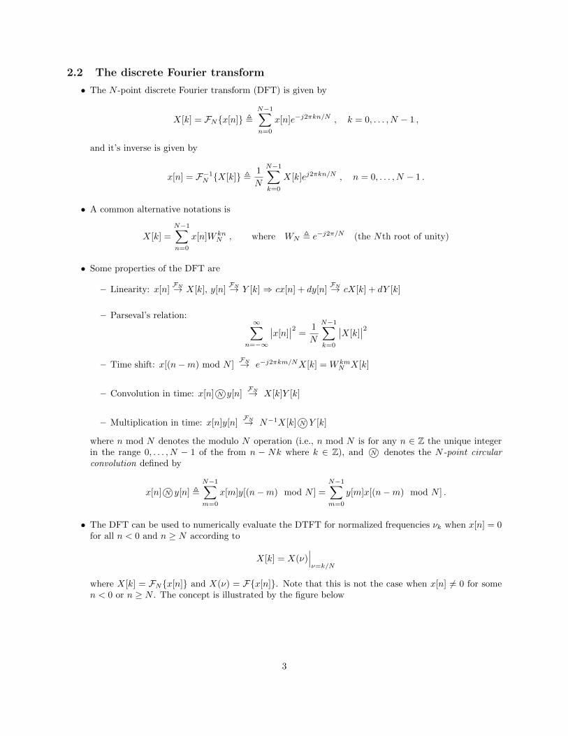
• The DFT can be used to numerically evaluate the DTFT for normalized frequencies νk when x[n] = 0for all n < 0 and n ≥ N according to
X[k] = X(ν)∣∣∣ν=k/N
where X[k] = FN{x[n]} and X(ν) = F{x[n]}. Note that this is not the case when x[n] 6= 0 for somen < 0 or n ≥ N . The concept is illustrated by the figure below
3
|X(ν)|
ν0 14
12
34
10
1
2
3
for the case where N = 4. Zero padding the DFT (increasing N beyond the minimum) can be usedto increase the number of normalized frequencies νk = k/N for k = 0, . . . , N − 1 where the DTFT isevaluated.
2.3 The fast Fourier transform
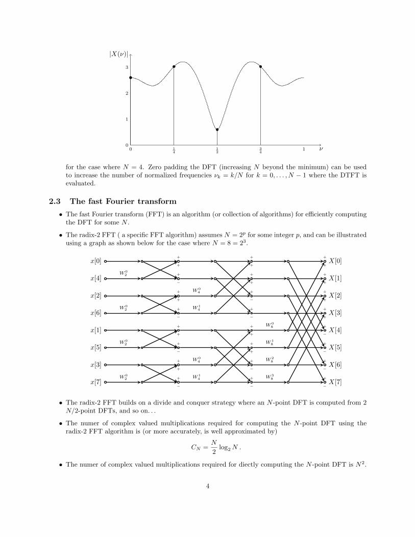
• The fast Fourier transform (FFT) is an algorithm (or collection of algorithms) for efficiently computingthe DFT for some N .
• The radix-2 FFT ( a specific FFT algorithm) assumes N = 2p for some integer p, and can be illustratedusing a graph as shown below for the case where N = 8 = 23.
X[0]
X[1]
X[2]
X[3]
X[4]
X[5]
X[6]
X[7]
+
+
+
+
+
+
+
+
+
−
+
−
+
−
+
−
W 08
W 18
W 28
W 38
+
+
+
+
+
−
+
−
+
+
+
+
+
−
+
−
W 04
W 14
W 04
W 14
+
+
+
−
+
+
+
−
+
+
+
−
+
+
+
−
W 02
W 02
W 02
W 02
x[0]
x[4]
x[2]
x[6]
x[1]
x[5]
x[3]
x[7]
• The radix-2 FFT builds on a divide and conquer strategy where an N -point DFT is computed from 2N/2-point DFTs, and so on. . .
• The numer of complex valued multiplications required for computing the N -point DFT using theradix-2 FFT algorithm is (or more accurately, is well approximated by)
CN =N
2log2N .
• The numer of complex valued multiplications required for diectly computing the N -point DFT is N2.
4
3 Filtering with the FFT
3.1 Linear and circular convolution
• The DFT can be used to filter finite length signals in the frequency domain by recognizing when thecyclic convolution computed the values of the linear convolution.
• Assume that x[n] has length L (x[n] = 0 if n < 0 or n ≥ L) and h[n] has length M (h[n] = 0 if n < 0or n ≥M). Let y[n] = h[n] ∗ x[n] and yN [n] = h[n] N x[n]. Then
y[n] = yN [n] for n = 0, . . . , N − 1
if N ≥ L+M −1. If N = L > M , then y[n] = yN [n] can only be guaranteed for n = M −1, . . . , N −1.
• The above results can be used to compute y[n] = h[n] ∗x[n] in the frequency domain from some valuesof n as yN [n] = F−1
N {FN{x[n]}×FN{h[n]}}. By using the FFT this can lead to fewer complex valuedmultiplications than the direct computation of y[n] via the convolution sum.
• The overall complexity in terms of complex valued multiplications can be broken down according to
– H[k] = FN{h[n]} : N/2 log2N multiplications
– X[k] = FN{x[n]} : N/2 log2N multiplications
– Y [k] = H[k]X[k] : N multiplications
– y[n] = F−1N {Y [k]} : N/2 log2N multiplications
which leads to a total complexity of
CN =3N log2N
2+N .
3.2 Overlap save and overlap add
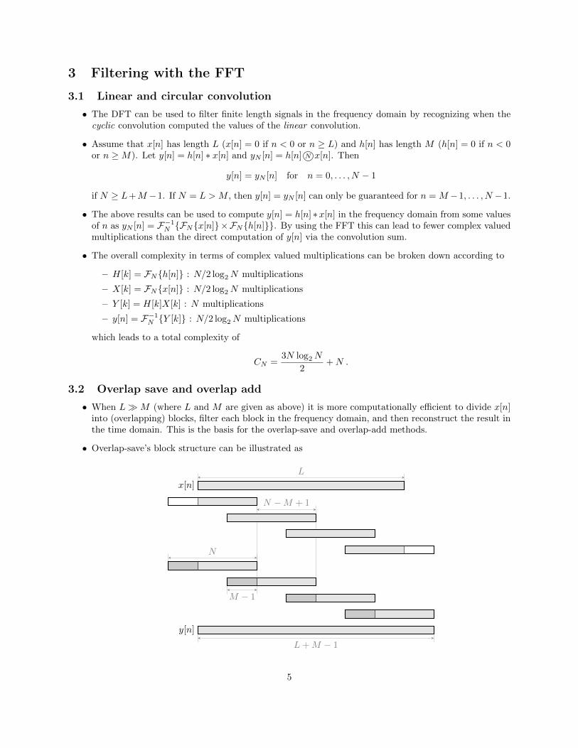
• When L�M (where L and M are given as above) it is more computationally efficient to divide x[n]into (overlapping) blocks, filter each block in the frequency domain, and then reconstruct the result inthe time domain. This is the basis for the overlap-save and overlap-add methods.
• Overlap-save’s block structure can be illustrated as
L
N −M + 1
x[n]
L+M − 1
N
M − 1
y[n]
5
• Overlap-add’s block structure can be illustrated as
L
N −M + 1
M − 1
x[n]
L+M − 1
N
y[n]
+
+
+
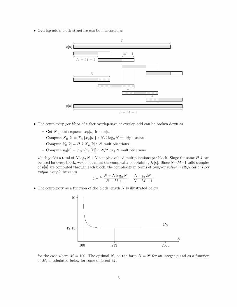
• The complexity per block of either overlap-save or overlap-add can be broken down as
– Get N -point sequence xB[n] from x[n]
– Compute XB[k] = FN{xB[n]} : N/2 log2N multiplications
– Compute YB[k] = H[k]XB [k] : N multiplications
– Compute yB[n] = F−1N {YB[k]} : N/2 log2N multiplications
which yields a total of N log2N+N complex valued multiplications per block. Singe the same H[k]canbe used for every block, we do not count the complexity of obtainingH[k]. SinceN−M+1 valid samplesof y[n] are computed through each block, the complexity in terms of complex valued multiplications peroutput sample becomes
CN ,N +N log2N
N −M + 1=
N log2 2N
N −M + 1.
• The complexity as a function of the block length N is illustrated below
N
100 833 2000
12.15
40
CN
for the case where M = 100. The optimal N , on the form N = 2p for an integer p and as a functionof M , is tabulated below for some different M .
6
M N CN5 16 6.6710 64 8.1515 64 8.9620 128 9.3950 512 11.06100 1024 12.181000 8192 15.94
4 FIR filters and FIR approximations
4.1 Overview
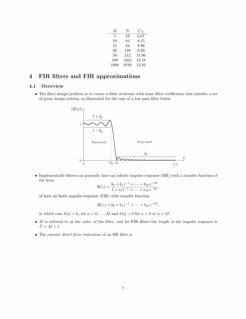
• The filter design problem is to create a filter structure with some filter coefficients that satisfies a setof given design criteria, as illustrated for the case of a low pass filter below.
1 + δp
1− δp
δs
νp νs
Pass band Stop band
1/200
1
ν
|H(ν)|
• Implementable filters can generally have an infinite impulse response (IIR) with a transfer function ofthe form
H(z) =b0 + b1z
−1 + · · ·+ bMz−M
1 + a1z−1 + · · ·+ aMz−M,
of have an finite impulse response (FIR) with transfer function
H(z) = b0 + b1z−1 + · · ·+ bMz
−M ,
in which case h[n] = bn for n = 0, . . . ,M and h[n] = 0 for n < 0 or n > M .
• M is referred to as the order of the filter, and for FIR filters the length of the impulse responce isN = M + 1.
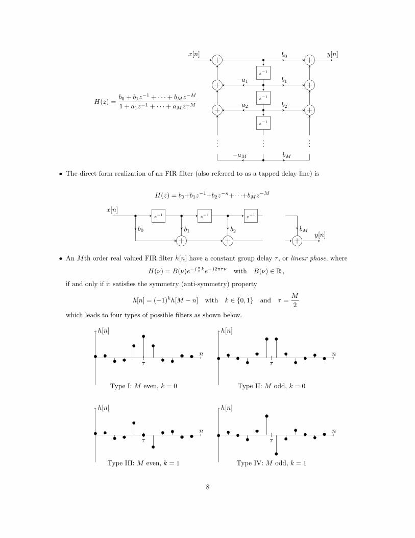
• The canonic direct form realization of an IIR filter is
7
+
+
+
+
+
+
z−1
z−1
z−1
b0
−a1 b1
−a2 b2
−aM bM
x[n] y[n]
......
...
H(z) =b0 + b1z
−1 + · · ·+ bMz−M
1 + a1z−1 + · · ·+ aMz−M
• The direct form realization of an FIR filter (also referred to as a tapped delay line) is
+ + +
z−1 z−1 z−1
b0 b1 b2 bM
x[n]
y[n]
H(z) = b0+b1z−1+b2z
−n+· · ·+bMz−M
• An Mth order real valued FIR filter h[n] have a constant group delay τ , or linear phase, where
H(ν) = B(ν)e−jπ2 ke−j2πτν with B(ν) ∈ R ,
if and only if it satisfies the symmetry (anti-symmetry) property
h[n] = (−1)kh[M − n] with k ∈ {0, 1} and τ =M
2
which leads to four types of possible filters as shown below.
h[n]
n
τ
Type I: M even, k = 0
h[n]
n
τ
Type II: M odd, k = 0
h[n]
n
τ
Type III: M even, k = 1
h[n]
n
τ
Type IV: M odd, k = 1
8
4.2 Frequency sampling
• The basic idea of frequency sampling can be described as follows.
1. Let D(ν) ∈ C be a desired frequency response, and select the filter length N
2. Let H[k] = D(k/N) for k = 0, . . . , N − 1
3. Obtain h[n] for k = 0, . . . , N − 1 by computing the N -point inverse DFT of H[k]
The resulting filter will always be FIR, but special care must be taken in the selection of D(ν) if onewish to to ensure that h[n] is real valued and has the linear phase property. Special design cases forthe different types of linear phase FIR filters are are given next.
• Type I linear phase Mth order FIR design (M even, symmetric filter): Let D(k/N) = A[k]e2πθ[k] withN = M + 1 and
θ[k] = − kM
2(M + 1)for k = 0, . . . ,M
A[k] = A[M − k + 1] for k = 1, . . . ,M/2
Then
h[n] =1
M + 1
A[0] + 2
M/2∑k=1
(−1)kA[k] cosπk(1 + 2n)
M + 1
, n = 0, . . . ,M
• Type II linear phase Mth order FIR design (M odd, symmetric filter): Let D(k/N) = A[k]e2πθ[k] withN = M + 1 and
θ[k] =
{− kM
2(M+1) for k = 0, . . . , (M − 1)/212 −
kM2(M+1) for k = (M + 3)/2, . . . ,M
A[k] = A[M − k + 1] for k = 1, . . . , (M + 1)/2
A[(M + 1)/2] = H(1/2) = 0
Then
h[n] =1
M + 1
A[0] + 2
(M−1)/2∑k=1
(−1)kA[k] cosπk(1 + 2n)
M + 1
, n = 0, . . . ,M
• Type III linear phase Mth order FIR design (M even, anti-symmetric filter): Let D(k/N) = A[k]e2πθ[k]
with N = M + 1 and
θ[k] =
{14 −
kM2(M+1) for k = 1, . . . ,M/2
− 14 −
kM2(M+1) for k = M/2 + 1, . . . ,M
A[k] = A[M − k + 1] for k = 1, . . . ,M/2
A[0] = H(0) = 0 , H(1/2) = 0
Then
h[n] =2
M + 1
M/2∑k=0
(−1)k+1A[k] sinπk(1 + 2n)
M + 1, n = 0, . . . ,M
9
• Type IV linear phase Mth order FIR design (M odd, anti-symmetric filter): Let D(k/N) = A[k]e2πθ[k]
with N = M + 1 and
θ[k] = −1
4− kM
2(M + 1)for k = 1, . . . ,M
A[k] = A[M − k + 1] for k = 1, . . . , (M + 1)/2
A[0] = H(0) = 0
Then
h[n] =1
M + 1
(−1)nA[(M + 1)/2] + 2
(M−1)/2∑k=0
(−1)kA[k] sinπk(1 + 2n)
M + 1
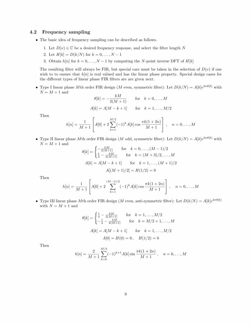
• An example of a Type I band stop filter of order M = 20 is given by
1/22/10 3/1000
1
1M+1
ν
|H(ν)|
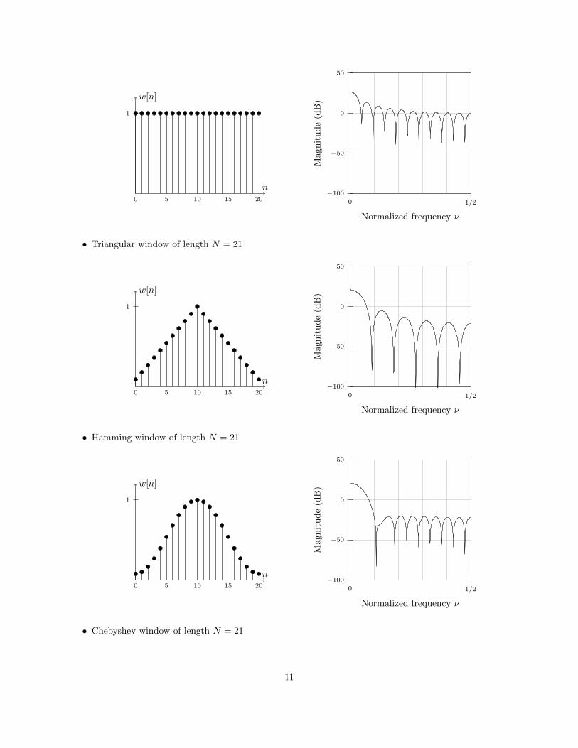
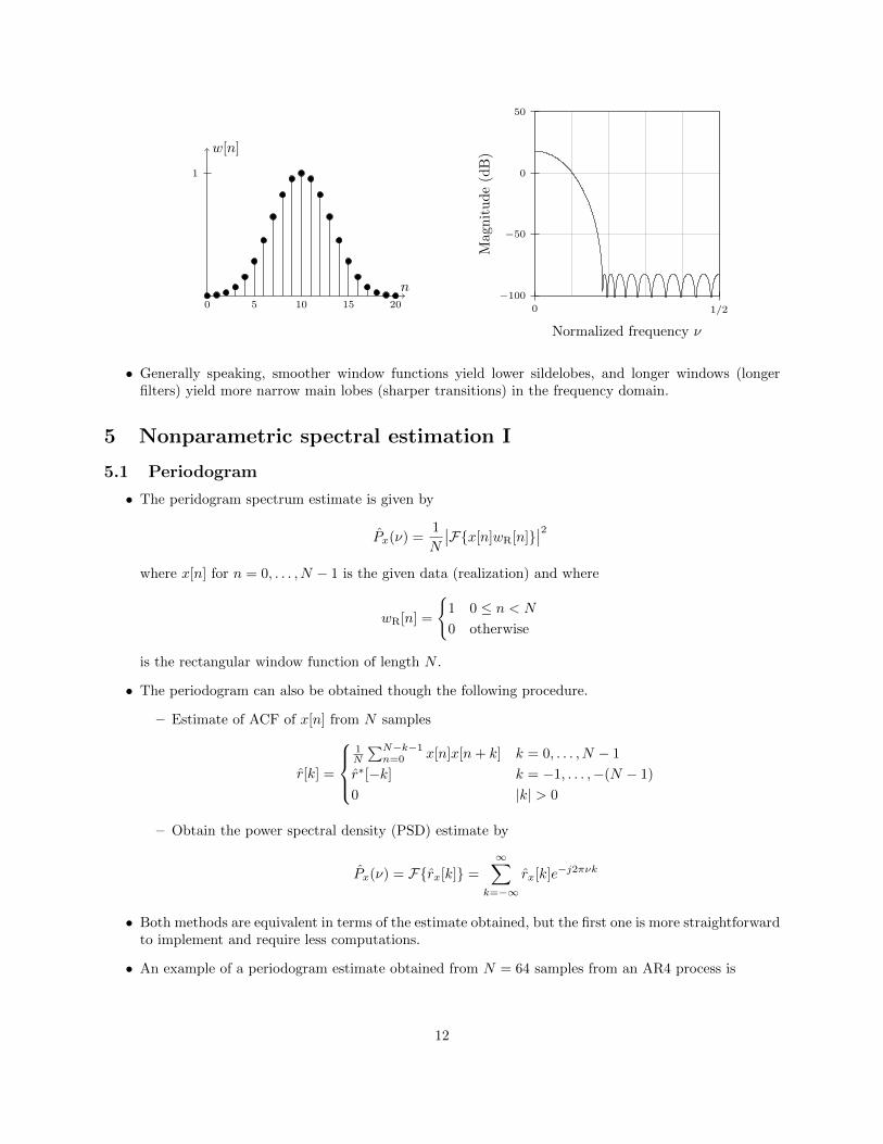
4.3 Windowing
• The creation of an order M FIR filter using the window method is given by
h[n] = hI[n]w[n]
where
– hI[n] is the ideal (desired) filter impulse response (typically infinite length)
– w[n] is the FIR window function, w[n] = 0 for n < 0 and n > M
• The resulting frequency response is given by
H(ν) = HI(ν) ~W (ν) =
∫ 1/2
−1/2
HI(ν − τ)W (τ)dτ ,
so the characteristics of the design are dictated by the window function (length and type)
• If the ideal response has linear phase, and the window function is real valued and symmetric, theresulting filter design will also have linear phase. Some example windows, and their DTFT (in dBscale) are given next.
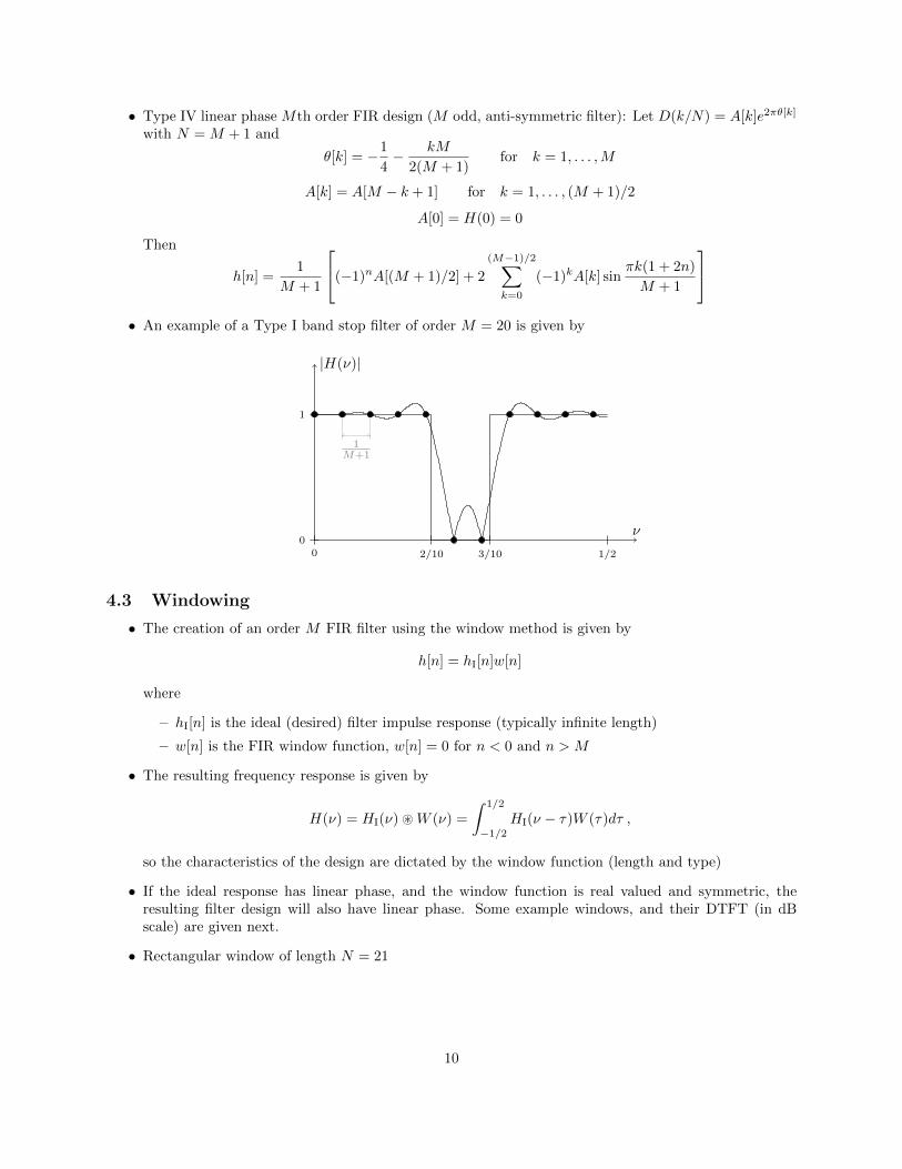
• Rectangular window of length N = 21
10
n
w[n]
1
0 5 10 15 20−100
−50
0
50
0 1/2
Normalized frequency ν
Mag
nit
ud
e(d
B)
• Triangular window of length N = 21
n
w[n]
1
0 5 10 15 20−100
−50
0
50
0 1/2
Normalized frequency ν
Mag
nit
ud
e(d
B)
• Hamming window of length N = 21
n
w[n]
1
0 5 10 15 20−100
−50
0
50
0 1/2
Normalized frequency ν
Mag
nit
ud
e(d
B)
• Chebyshev window of length N = 21
11
n
w[n]
1
0 5 10 15 20−100
−50
0
50
0 1/2
Normalized frequency ν
Mag
nit
ud
e(d
B)
• Generally speaking, smoother window functions yield lower sildelobes, and longer windows (longerfilters) yield more narrow main lobes (sharper transitions) in the frequency domain.
5 Nonparametric spectral estimation I
5.1 Periodogram
• The peridogram spectrum estimate is given by
Px(ν) =1
N
∣∣F{x[n]wR[n]}∣∣2
where x[n] for n = 0, . . . , N − 1 is the given data (realization) and where
wR[n] =
{1 0 ≤ n < N
0 otherwise
is the rectangular window function of length N .
• The periodogram can also be obtained though the following procedure.
– Estimate of ACF of x[n] from N samples
r[k] =
1N
∑N−k−1n=0 x[n]x[n+ k] k = 0, . . . , N − 1
r∗[−k] k = −1, . . . ,−(N − 1)
0 |k| > 0
– Obtain the power spectral density (PSD) estimate by
Px(ν) = F{rx[k]} =
∞∑k=−∞
rx[k]e−j2πνk
• Both methods are equivalent in terms of the estimate obtained, but the first one is more straightforwardto implement and require less computations.
• An example of a periodogram estimate obtained from N = 64 samples from an AR4 process is
12
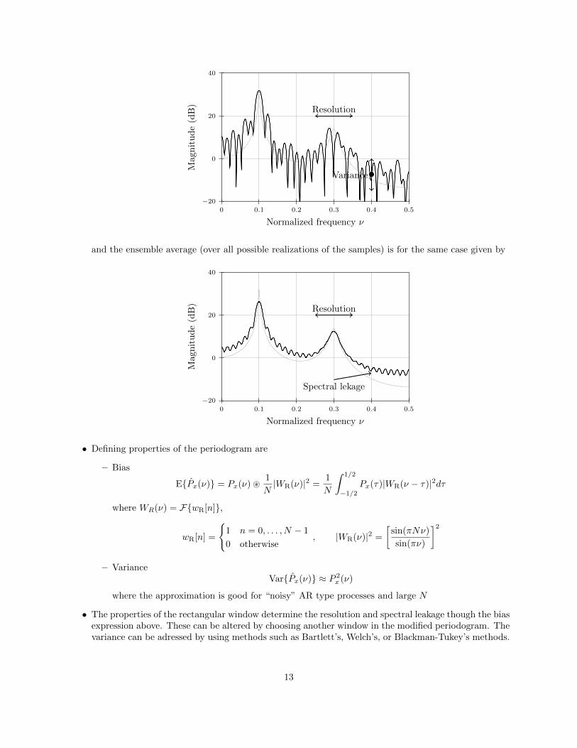
−20
0
20
40
0 0.1 0.2 0.3 0.4 0.5
Normalized frequency ν
Magn
itu
de
(dB
) Resolution
Variance
and the ensemble average (over all possible realizations of the samples) is for the same case given by
−20
0
20
40
0 0.1 0.2 0.3 0.4 0.5
Normalized frequency ν
Mag
nit
ud
e(d
B) Resolution
Spectral lekage
• Defining properties of the periodogram are
– Bias
E{Px(ν)} = Px(ν) ~1
N|WR(ν)|2 =
1
N
∫ 1/2
−1/2
Px(τ)|WR(ν − τ)|2dτ
where WR(ν) = F{wR[n]},
wR[n] =
{1 n = 0, . . . , N − 1
0 otherwise, |WR(ν)|2 =
[sin(πNν)
sin(πν)
]2
– VarianceVar{Px(ν)} ≈ P 2
x (ν)
where the approximation is good for “noisy” AR type processes and large N
• The properties of the rectangular window determine the resolution and spectral leakage though the biasexpression above. These can be altered by choosing another window in the modified periodogram. Thevariance can be adressed by using methods such as Bartlett’s, Welch’s, or Blackman-Tukey’s methods.
13
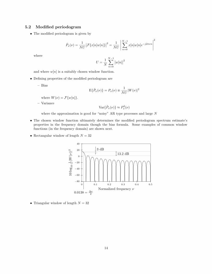
5.2 Modified periodogram
• The modified periodogram is given by
Px(ν) =1
NU
∣∣F{x[n]w[n]}∣∣2 =
1
NU
∣∣∣∣∣N−1∑n=0
x[n]w[n]e−j2πνn
∣∣∣∣∣2
where
U =1
N
N−1∑n=0
∣∣w[n]∣∣2
and where w[n] is a suitably chosen window function.
• Defining properties of the modified periodogram are
– Bias
E{Px(ν)} = Px(ν) ~1
NU|W (ν)|2
where W (ν) = F{w[n]}.– Variance
Var{Px(ν)} ≈ P 2x (ν)
where the approximation is good for “noisy” AR type processes and large N
• The chosen window function ultimately determines the modified periodogram spectrum estimate’sproperties in the frequency domain though the bias formula. Some examples of common windowfunctions (in the frequency domain) are shown next.
• Rectangular window of length N = 32
−80
−60
−40
−20
0
20
40
0 0.1 0.2 0.3 0.4 0.5
Normalized frequency ν
10lo
g10
1 U|W
(ν)|2
3 dB
13.2 dB
0.0138 = ∆ν2
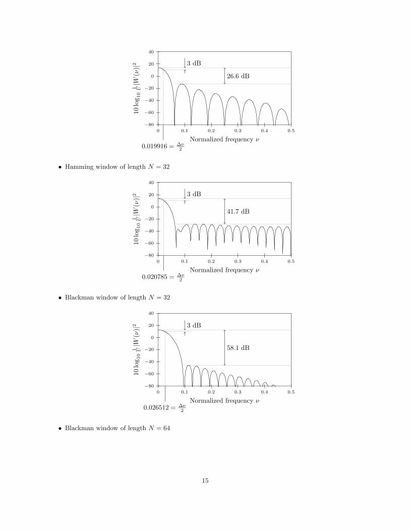
• Triangular window of length N = 32
14
−80
−60
−40
−20
0
20
40
0 0.1 0.2 0.3 0.4 0.5
Normalized frequency ν10
log
10
1 U|W
(ν)|2 3 dB
26.6 dB
0.019916 = ∆ν2
• Hamming window of length N = 32
−80
−60
−40
−20
0
20
40
0 0.1 0.2 0.3 0.4 0.5
Normalized frequency ν
10lo
g10
1 U|W
(ν)|2 3 dB
41.7 dB
0.020785 = ∆ν2
• Blackman window of length N = 32
−80
−60
−40
−20
0
20
40
0 0.1 0.2 0.3 0.4 0.5
Normalized frequency ν
10lo
g10
1 U|W
(ν)|2 3 dB
58.1 dB
0.026512 = ∆ν2
• Blackman window of length N = 64
15
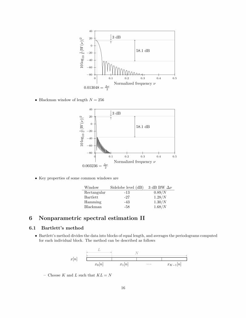
−80
−60
−40
−20
0
20
40
0 0.1 0.2 0.3 0.4 0.5
Normalized frequency ν10
log
10
1 U|W
(ν)|2
3 dB
58.1 dB
0.013048 = ∆ν2
• Blackman window of length N = 256
−80
−60
−40
−20
0
20
40
0 0.1 0.2 0.3 0.4 0.5
Normalized frequency ν
10lo
g10
1 U|W
(ν)|2
3 dB
58.1 dB
0.003236 = ∆ν2
• Key properties of some common windows are
Window Sidelobe level (dB) 3 dB BW ∆νRectangular -13 0.89/NBartlett -27 1.28/NHamming -43 1.30/NBlackman -58 1.68/N
6 Nonparametric spectral estimation II
6.1 Bartlett’s method
• Bartlett’s method divides the data into blocks of equal length, and averages the periodograms computedfor each individual block. The method can be described as follows
N
x[n]
L
x0[n] x1[n] · · · xK−1[n]
– Choose K and L such that KL = N
16
– Create K length L blocks xk[n] = x[kL+ n], n = 0, . . . , L− 1, k = 0, . . . ,K − 1
– Average length L periodograms to get
PBx (ν) =
1
K
K−1∑k=0
1
L
∣∣F{xk[n]}∣∣2
• Defining properties of Bartlett’s method are
– Bias
E{PBx (ν)} = Px(ν) ~
1
L|W (L)
R (ν)|2 where W(L)R (ν) =
sin(πLν)
sin(πν)
– Variance
Var{PBx (ν)} ≈ 1
KP 2x (ν)
where the approximation is good for “noisy” AR type processes and sufficiently large L
– The resolution is the same as for the length L periodogram
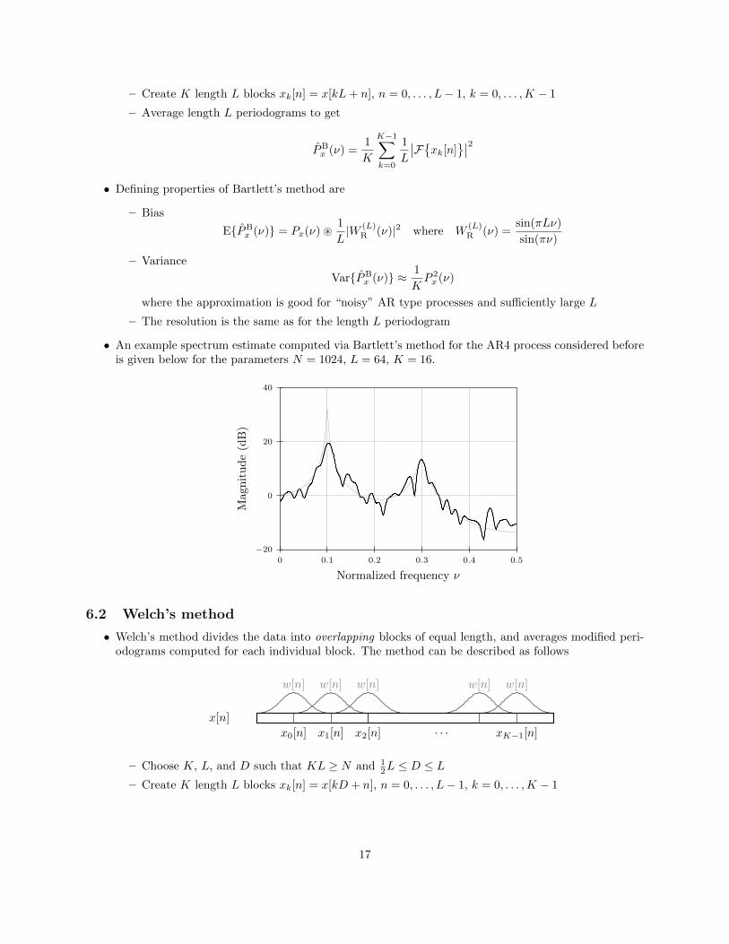
• An example spectrum estimate computed via Bartlett’s method for the AR4 process considered beforeis given below for the parameters N = 1024, L = 64, K = 16.
−20
0
20
40
0 0.1 0.2 0.3 0.4 0.5
Normalized frequency ν
Mag
nit
ud
e(d
B)
6.2 Welch’s method
• Welch’s method divides the data into overlapping blocks of equal length, and averages modified peri-odograms computed for each individual block. The method can be described as follows
w[n] w[n] w[n] w[n] w[n]
x[n]
x0[n] x1[n] x2[n] · · · xK−1[n]
– Choose K, L, and D such that KL ≥ N and 12L ≤ D ≤ L
– Create K length L blocks xk[n] = x[kD + n], n = 0, . . . , L− 1, k = 0, . . . ,K − 1
17
– Average length L modified periodograms to get
PWx (ν) =
1
K
K−1∑k=0
1
LU
∣∣F{xk[n]w[n]}∣∣2 , U =
1
L
L−1∑n=0
w2[n] .
• Defining properties of Welch’s method are
– Bias
E{PWx (ν)} = Px(ν) ~
1
LU|W (L)(ν)|2 where W (L)(ν) = F{w[n]}
– Variance (assuming a triangular window and 50% overlap)
Var{PWx (ν)} ≈ 9
8KP 2x (ν)
where the approximation is good for “noisy” AR type processes and sufficiently large L
– The resolution is the same as for the length L modified periodogram
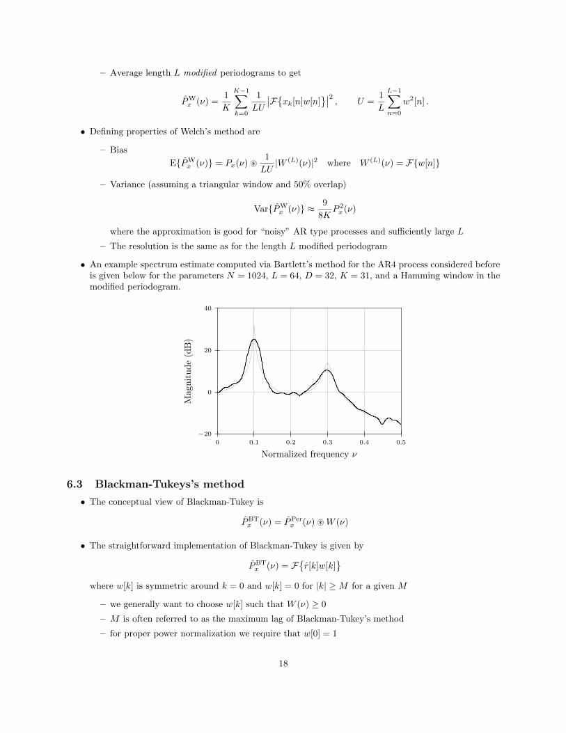
• An example spectrum estimate computed via Bartlett’s method for the AR4 process considered beforeis given below for the parameters N = 1024, L = 64, D = 32, K = 31, and a Hamming window in themodified periodogram.
−20
0
20
40
0 0.1 0.2 0.3 0.4 0.5
Normalized frequency ν
Mag
nit
ud
e(d
B)
6.3 Blackman-Tukeys’s method
• The conceptual view of Blackman-Tukey is
PBTx (ν) = PPer
x (ν) ~W (ν)
• The straightforward implementation of Blackman-Tukey is given by
PBTx (ν) = F
{r[k]w[k]
}where w[k] is symmetric around k = 0 and w[k] = 0 for |k| ≥M for a given M
– we generally want to choose w[k] such that W (ν) ≥ 0
– M is often referred to as the maximum lag of Blackman-Tukey’s method
– for proper power normalization we require that w[0] = 1
18
• Defining properties of Blackman-Tukey’s method are
– BiasE{PBT
x (ν)} ≈ Px(ν) ~W (2M+1)(ν) where W (2M+1)(ν) = F{w[n]}
– Variance
Var{PBTx (ν)} ≈
[1
N
M∑k=−M
w2[k]
]P 2x (ν)
where the approximation is good for “noisy” AR type processes.
– The reduction for the variance can be computed explicitly as
1
N
M∑k=−M
w2[k] =
{2M/N rectangular window
2M/3N triangular window
– The resolution is proportional to 1/M and ultimately determined by the window function used
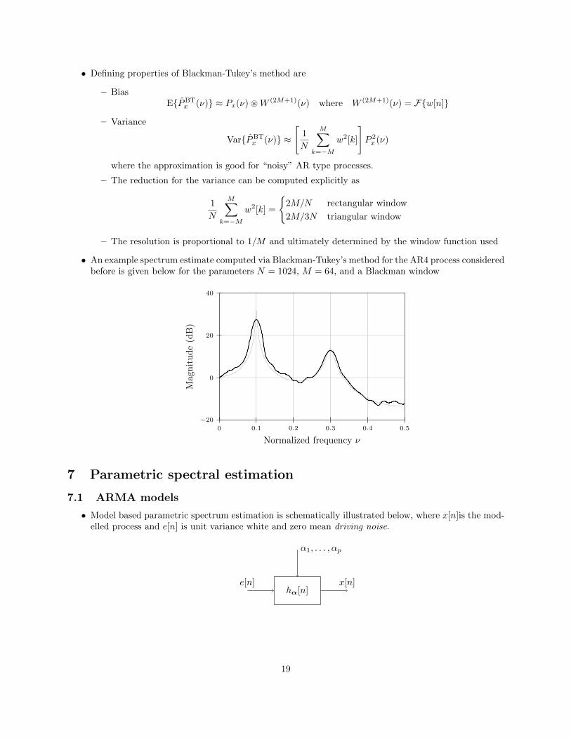
• An example spectrum estimate computed via Blackman-Tukey’s method for the AR4 process consideredbefore is given below for the parameters N = 1024, M = 64, and a Blackman window
−20
0
20
40
0 0.1 0.2 0.3 0.4 0.5
Normalized frequency ν
Mag
nit
ud
e(d
B)
7 Parametric spectral estimation
7.1 ARMA models
• Model based parametric spectrum estimation is schematically illustrated below, where x[n]is the mod-elled process and e[n] is unit variance white and zero mean driving noise.
hα[n]e[n] x[n]
α1, . . . , αp
19
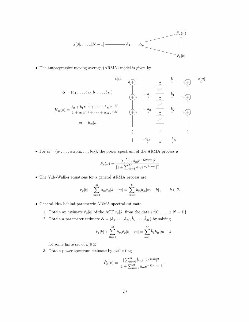
x[0], . . . , x[N − 1] α1, . . . , αp
Px(ν)
rx[k]
• The autoregressive moving average (ARMA) model is given by
+
+
+
+
+
+
z−1
z−1
z−1
b0
−a1 b1
−a2 b2
−aM bM
e[n] x[n]
......
...
α = (a1, . . . , aM , b0, . . . , bM )
Hα(z) =b0 + b1z
−1 + · · ·+ bMz−M
1 + a1z−1 + · · ·+ aMz−M
⇒ hα[n]
• For α = (a1, . . . , aM , b0, . . . , bM ), the power spectrum of the ARMA process is
Px(ν) =|∑Mm=0 bme
−j2πνm|2
|1 +∑Mm=1 ame
−j2πνm|2
• The Yule-Walker equations for a general ARMA process are
rx[k] +
M∑m=1
amrx[k −m] =
M∑m=0
bmhα[m− k] , k ∈ Z
• General idea behind parametric ARMA spectral estimate
1. Obtain an estimate rx[k] of the ACF rx[k] from the data {x[0], . . . , x[N − 1]}
2. Obtain a parameter estimate α = (a1, . . . , aM , b0, . . . , bM ) by solving
rx[k] +
M∑m=1
amrx[k −m] =
M∑k=0
bkhα[m− k]
for some finite set of k ∈ Z3. Obtain power spectrum estimate by evaluating
Px(ν) =|∑Mm=0 bme
−j2πνm|2
|1 +∑Mm=1 ame
−j2πνm|2.
20

7.2 AR models
• The purely autoregressive (AR) model is given by
+
+
+
z−1
z−1
z−1
b0 x[n]
−a1
−a2
−aM
e[n]
......
α = (a1, . . . , aM , b0)
Hα(z) =b0
1 + a1z−1 + · · ·+ aMz−M
⇒ hα[n]
• The Yule-Walker equations for pure AR process are
rx[k] +
M∑m=1
amrx[k −m] = b20δ[k] , k ∈ Z
which for k = 1, . . . ,M simplifies to
rx[k] +
M∑m=1
amrx[k −m] = 0 ,
which can be used to solve for a1, . . . , aM , and which for k = 0 simplifies to
b0 =
√√√√rx[0] +
M∑m=1
amrx[m] ,
which yields b0.
• The autocorrelation method estimates the autocorrelation according to
r[k] =
1N
∑N−k−1n=0 x[n]x[n+ k] k = 0, . . . , N − 1
r[−k] k = −1, . . . ,−(N − 1)
0 |k| > |N |
and solves the Yule-Walker equations with rx[k] in place of rx[k] for estimates of the model parametersa1, . . . , aM , b0), for some model order M under the assumption that N ≥M .
7.3 MMSE prediction
• Consider the problem of estimating a random variable y ∈ R from a random vector x ∈ Rn.
– A linear detector has the form y = wTx where w ∈ Rn is a set of weights.
21

– The best linear detector, in the mean square sense, is given by the solution to
Rxw = ryx ⇔ w = R−1x ryx
where Rx = E{xxT} and ryx = E{yx} .
– The minimum mean square error (MSE) is given by
E{y2} − rTyxR
−1x ryx
• The coefficients w ∈ RM of the Mth order linear minimum mean square error 1-step ahead predictorare related to the ARM parameters a ∈ RM as w = −a. Moreover, for the ARM model we have
b20 = rx[0] +
M∑m=1
amrx[m] = rx[0] + aTryx
and for the 1-step ahead predictor we have
MSE = E{y2} − rTyxR
−1x ryx = E{y2} −wTryx
if w = R−1x ryx, which implies that b20 = MSE because E{y2} = rx[0] and w = −a.
• One may choose AR model order by increasing M until no significant further reduction in b20 is observed.
• Assume that N is the number of data-samples, and b20,M is driving noise power for the M -th order ARmodel, then two famous model order selection criteria are
– Akaike information criterion (AIC): Choose M to minimize
AIC(M) = ln b20,M +2M
N
– Minimum description length (MDL): Choose M to minimize
MDL(M) = N ln b20,M +M lnN
8 Multirate signal processing: Decimation and Interpolation
8.1 Downsampling
• Downsampling by an integer factor of D is the operation given by
y[m] = x[mD] ∀m ∈ Z ,
which is schematically drawn as
↓ Dx[n] y[m]
• In terms of the DTFT it holds that
Y (ν) =1
D
D−1∑k=0
X
(ν − kD
).
22
• In terms of the bilateral z-transform it holds that
Y (z) =1
D
D−1∑k=0
X(z1/De−j2πk/D
).
• Proper decimation refers to the operation
↓ Dh[n]x[n] z[n] y[m]
wherez[n] = h[n] ∗ x[n] , y[m] = z[mD] ∀m ∈ Z
and
F{h[n]} = H(ν) =
{1 |ν| ≤ 1
2D
0 12D ≤ |ν| ≤
12
• For proper decimation it holds that
Y (ν) =1
DX( νD
), |ν| ≤ 1
2,
and for a general (possibly imperfect) decimation filter with frequency response H(ν) it holds that
Y (ν) =1
D
D−1∑k=0
H
(ν − kD
)X
(ν − kD
).
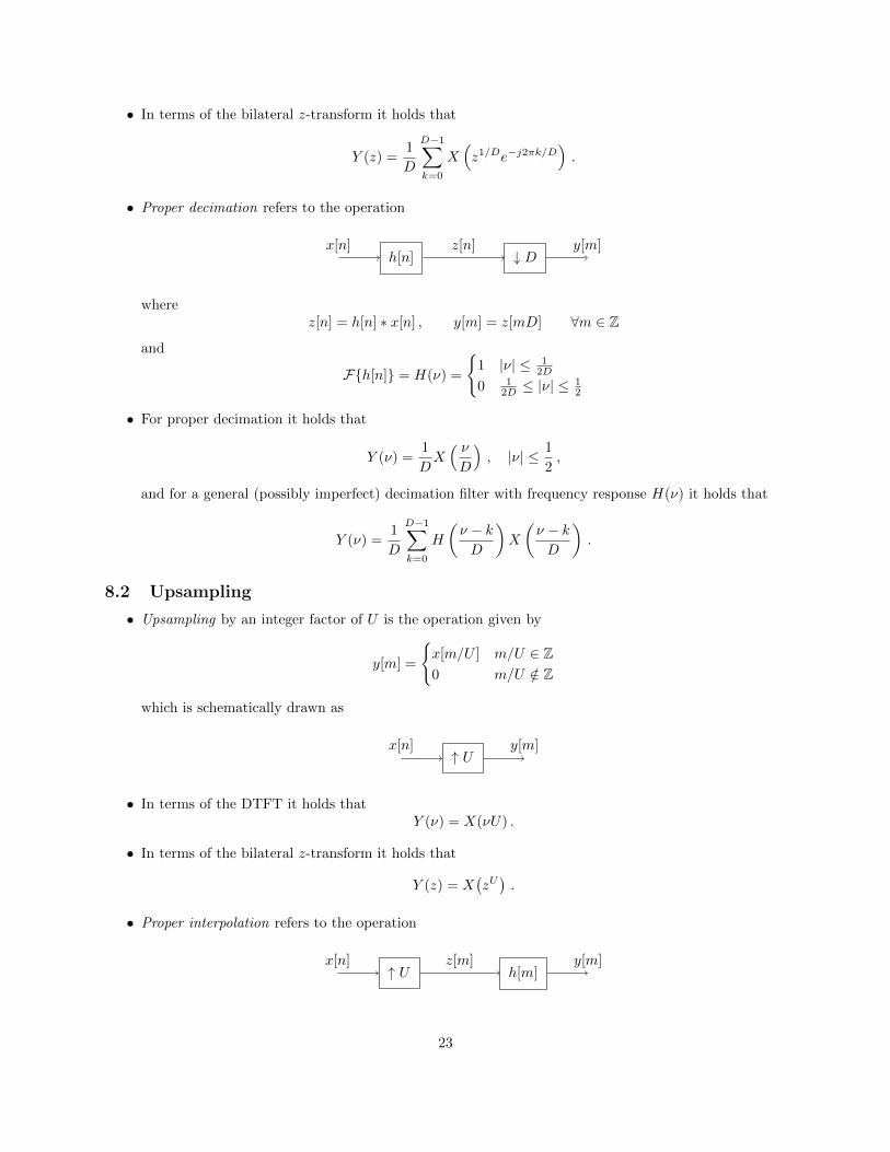
8.2 Upsampling
• Upsampling by an integer factor of U is the operation given by
y[m] =
{x[m/U ] m/U ∈ Z0 m/U /∈ Z
which is schematically drawn as
↑ Ux[n] y[m]
• In terms of the DTFT it holds thatY (ν) = X(νU) .
• In terms of the bilateral z-transform it holds that
Y (z) = X(zU).
• Proper interpolation refers to the operation
↑ U h[m]x[n] z[m] y[m]
23

where
z[m] =
{x[m/U ] m/U ∈ Z0 m/U /∈ Z
, y[m] = h[m] ∗ z[m] ∀m ∈ Z
and
F{h[m]} = H(ν) =
{U |ν| ≤ 1
2U
0 12U ≤ |ν| ≤
12
• For proper interpolation it holds that
Y (ν) =
{UX(Uν) |ν| ≤ 1
2U
0 12U ≤ |ν| ≤
12
,
and for a general (possibly imperfect) interpolation filter with frequency response H(ν) it holds that
Y (ν) = H(ν)X(Uν) .
8.3 Upsampling and downsampling stochastic signals
• Downsampling a wide sense stationary signal x[n] to y[m] with a factor D gives
Py(ν) =1
D
D−1∑k=0
Px
(ν − kD
)
• Decimating x[n] to y[m] with a filter H(ν) gives
Py(ν) =1
D
D−1∑k=0
Px
(ν − kD
) ∣∣∣∣H (ν − kD
)∣∣∣∣2
• Proper decimation with a factor D gives
Py(ν) =1
DPx
( νD
), |ν| ≤ 1
2D
• Upsampling a wide sense stationary signal x[n] to y[m] with a factor U gives (after the inclusion of auniform random time delay Θ ∼ U [0, 1, . . . , U − 1] needed to ensure wide sense stationarity in y[m])
Py(ν) =1
UPx(Uν)
• Interpolating x[n] to y[m] with a filter H(ν) gives
Py(ν) =1
UPx(Uν)|H(ν)|2
• Proper interpolation with a factor U gives
Py(ν) =
{UPx(Uν) |ν| ≤ 1
2U
0 12U ≤ |ν| ≤
12
24
9 Multirate signal processing: Filter banks
9.1 Filterbanks
• A two branch filterbank, with the task of splitting the signal x[n] into two half rate signals v0[m] andv1[m] typically representing the low and high frequency content of the signal repspectively, is illustatedbelow.
+H0(ν) ↓ 2 ↑ 2 G0(ν)x[n] v0[m] y[n]
H1(ν) ↓ 2 ↑ 2 G1(ν)v1[m]
• The input output relation of a two branch filter bank is under the bilateral z-transform given by
Y (z) =1
2
[G0(z)H0(z) +G1(z)H1(z)
]X(z)
+1
2
[G0(z)H0(−z) +G1(z)H1(−z)
]X(−z)︸ ︷︷ ︸
aliasing
.
• Perfect reconstruction with delay L, i.e., y[n] = x[n− L], is achieved if
G0(z)H0(z) +G1(z)H1(z) = 2z−L
G0(z)H0(−z) +G1(z)H1(−z) = 0
• The symmetry assumptions G0(z) = H1(−z) and G1(z) = −H0(−z) are sufficient conditions for aliascanceling.
• The quadrature mirror filter (QMF) design satisfies the symmetry assumptions above with the filterschosen as H0(z) = H(z), H1(z) = H(−z), G0(z) = H(z) and G1(z) = −H(−z) for some base (typicallylow pass) filter H(z).
9.2 Polyphase implementations
• The polyphase implementation of a decimation circuit with downsampling factor D and decimation(anti aliasing) filter h[n] is shown below.
↓ Dx[n]
z−1
↓ D
z−1
↓ D
p0[n]
p1[n]
p2[n]
+
+
y[m]
...
pk[n] = h[Dn+ k]
25
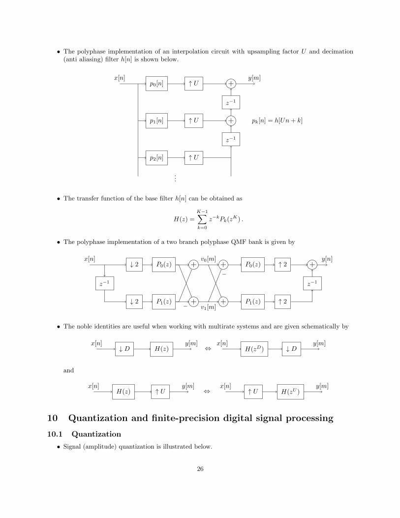
• The polyphase implementation of an interpolation circuit with upsampling factor U and decimation(anti aliasing) filter h[n] is shown below.
p0[n]x[n]
p1[n]
p2[n]
↑ U
↑ U
↑ U
+
+
z−1
z−1
y[m]
...
pk[n] = h[Un+ k]
• The transfer function of the base filter h[n] can be obtained as
H(z) =
K−1∑k=0
z−kPk(zK) .
• The polyphase implementation of a two branch polyphase QMF bank is given by
↓ 2
↓ 2
z−1
P0(z)
P1(z)
+
+
+
+
P0(z)
P1(z)
↑ 2
↑ 2
z−1
+x[n]
−
v0[m]
v1[m]
−
y[n]
• The noble identities are useful when working with multirate systems and are given schematically by
↓ D H(z)x[n] y[m]
⇔ ↓ DH(zD)x[n] y[m]
and
↑ UH(z)x[n] y[m]
⇔ ↑ U H(zU )x[n] y[m]
10 Quantization and finite-precision digital signal processing
10.1 Quantization
• Signal (amplitude) quantization is illustrated below.
26
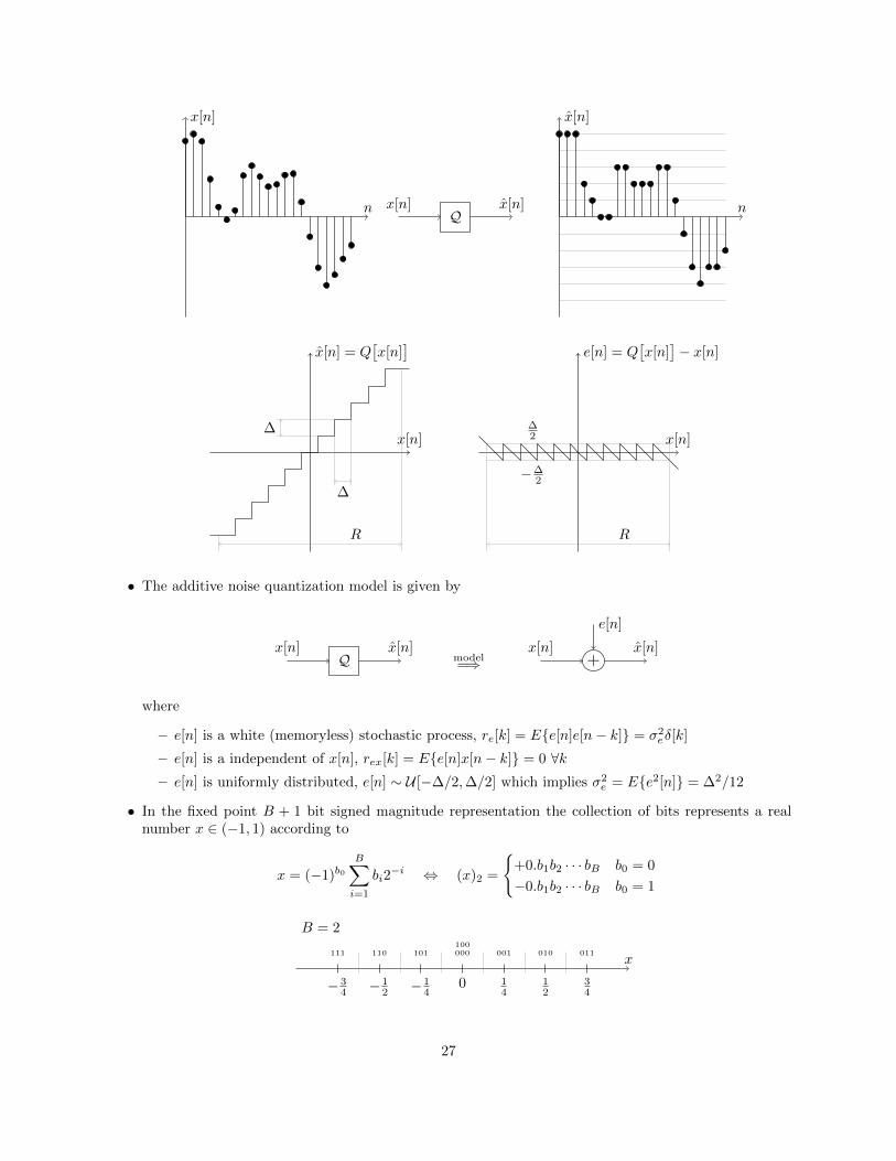
n
x[n]
n
x[n]
Qx[n] x[n]
x[n]
x[n] = Q[x[n]
]
∆
∆
R
x[n]
e[n] = Q[x[n]
]− x[n]
∆2
−∆2
R
• The additive noise quantization model is given by
Qx[n] x[n]
model=⇒ +
x[n]
e[n]
x[n]
where
– e[n] is a white (memoryless) stochastic process, re[k] = E{e[n]e[n− k]} = σ2eδ[k]
– e[n] is a independent of x[n], rex[k] = E{e[n]x[n− k]} = 0 ∀k– e[n] is uniformly distributed, e[n] ∼ U [−∆/2,∆/2] which implies σ2
e = E{e2[n]} = ∆2/12
• In the fixed point B + 1 bit signed magnitude representation the collection of bits represents a realnumber x ∈ (−1, 1) according to
x = (−1)b0B∑i=1
bi2−i ⇔ (x)2 =
{+0.b1b2 · · · bB b0 = 0
−0.b1b2 · · · bB b0 = 1
x
B = 2
0 14
12
34− 1
4− 12− 3
4
000100
001 010 011101110111
27
• In the fixed point B + 1 we have ∆ = 2−B and
σ2e =
∆2
12.
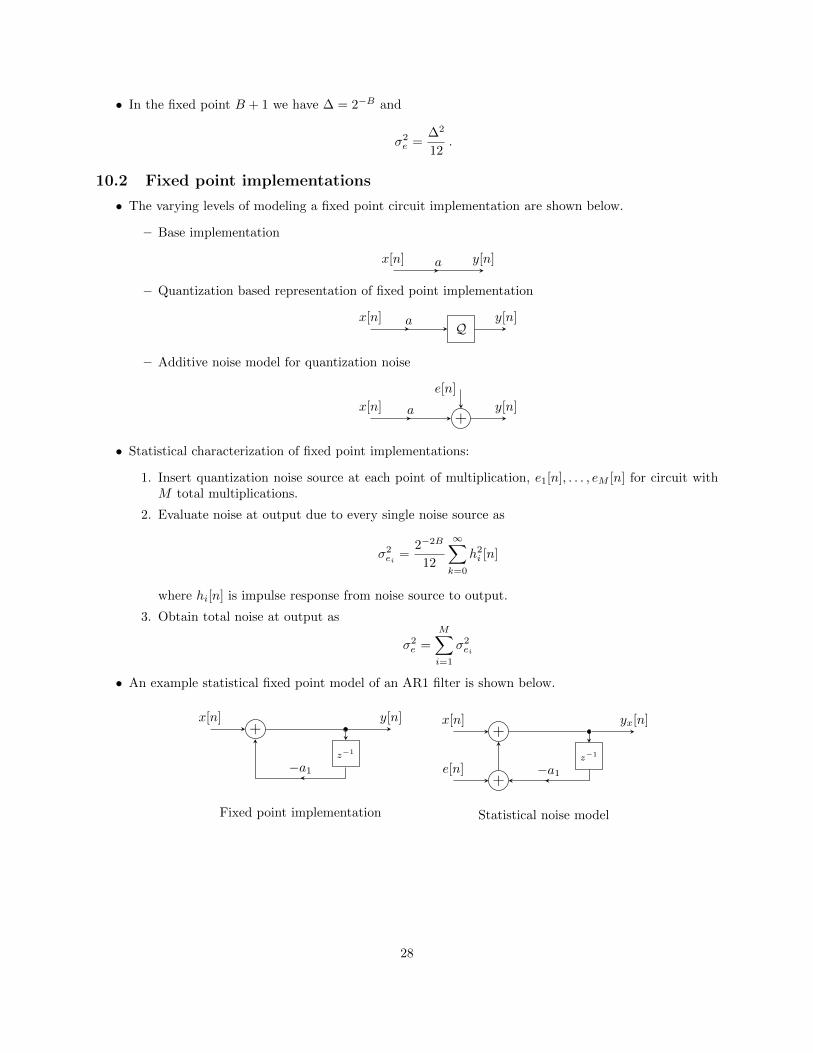
10.2 Fixed point implementations
• The varying levels of modeling a fixed point circuit implementation are shown below.
– Base implementation
y[n]x[n] a
– Quantization based representation of fixed point implementation
Qx[n] a y[n]
– Additive noise model for quantization noise
+x[n] a y[n]
e[n]
• Statistical characterization of fixed point implementations:
1. Insert quantization noise source at each point of multiplication, e1[n], . . . , eM [n] for circuit withM total multiplications.
2. Evaluate noise at output due to every single noise source as
σ2ei =
2−2B
12
∞∑k=0
h2i [n]
where hi[n] is impulse response from noise source to output.
3. Obtain total noise at output as
σ2e =
M∑i=1
σ2ei
• An example statistical fixed point model of an AR1 filter is shown below.
+
+
z−1
y[n]
−a1
x[n]
Fixed point implementation
+
+
z−1
yx[n]
−a1
x[n]
e[n]
Statistical noise model
28

11 Fixed point filter implementations
11.1 Filter coefficient quantization
• A Type I linear phase FIR filter can be constructed as a cascade of smaller components of the form
– Second order “Type I” component
Hk(z) = ck0 + ck1z−1 + ck0z
−2
– Fourth order “Type I” component
Hk(z) = ck0 + ck1z−1 + ck2z
−2 + ck1z−3 + ck0z
−4
– These components are sufficient for realizing all Type I linear phase FIR filters
– Quantization of cki, i = 0, . . . , 2, maintains linear phase property
• For second order Type I factors, the transfer function
Hk(z) = ck0 + ck1z−1 + ck0z
−2 ,
where ck0, ck1 ∈ R , if zk is a complex valued zero, Hk(zk) = 0 and ={zk} 6= 0, then Hk(z∗k) = 0 and|zk| = 1.
• For fourth order Type I factors, the transfer function
Hk(z) = ck0 + ck1z−1 + ck2z
−2 + ck1z−3 + ck0z
−4
where ck0, ck1, ck2 ∈ R , if zk is a complex valued zero, Hk(zk) = 0 and ={zk} 6= 0, then Hk(z∗k) = 0,Hk(1/zk) = 0, and Hk(1/z∗k) = 0.
11.2 Circuit sensitivity
• The sensitivity of H(z) to perturbations in a filter coefficient mk is given by
∂
∂mkH(z) = Fk(z)Gk(z)
– Fk(z) is the transfer function from the input to before the multiplication
– Gk(z) is the transfer function from an input after the multiplication to the output
x[n] y[n] + ∆y[n]
+mk
u[n] v[n]∆mk
Transfer functions: x[n]→ u[n] : Fk(z) , v[n]→ y[n] : Gk(z)
29
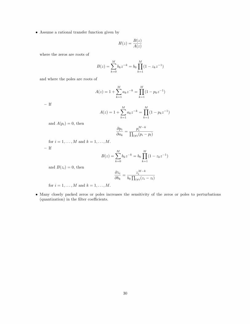
• Assume a rational transfer function given by
H(z) =B(z)
A(z)
where the zeros are roots of
B(z) =
M∑k=0
bkz−k = b0
M∏k=1
(1− zkz−1)
and where the poles are roots of
A(z) = 1 +
M∑k=1
akz−k =
M∏k=1
(1− pkz−1)
– If
A(z) = 1 +
M∑k=1
akz−k =
M∏k=1
(1− pkz−1)
and A(pi) = 0, then
∂pi∂ak
=pM−ki∏
l 6=i(pi − pl)
for i = 1, . . . ,M and k = 1, . . . ,M .
– If
B(z) =
M∑k=0
bkz−k = b0
M∏k=1
(1− zkz−1)
and B(zi) = 0, then
∂zi∂bk
=zM−ki
b0∏l 6=i(zi − zl)
for i = 1, . . . ,M and k = 1, . . . ,M .
• Many closely packed zeros or poles increases the sensitivity of the zeros or poles to perturbations(quantization) in the filter coefficients.
30