TCS -TR-A-12-59

TCS Technical Report

Loss Minimization of Power Distribution Networks

with Guaranteed Error Bound

by

Takeru Inoue, Keiji Takano, Takayuki Watanabe,

Jun Kawahara, Ryo Yoshinaka, Akihiro Kishimoto,

Koji Tsuda, Shin-ichi Minato, Yasuhiro Hayashi

Division of Computer Science

Report Series A

August 21, 2012

Hokkaido UniversityGraduate School of

Information Science and Technology

Email: minato@ist.hokudai.ac.jp Phone: +81-011-706-7682

Fax: +81-011-706-7682

Loss Minimization of Power Distribution Networks

with Guaranteed Error Bound

Takeru Inoue ∗ Keiji Takano † Takayuki Watanabe ‡

Jun Kawahara ∗ Ryo Yoshinaka § Akihiro Kishimoto †

Koji Tsuda ¶ ∗ Shin-ichi Minato ‖ ∗ Yasuhiro Hayashi ‡

August 21, 2012

Abstract

Determining loss minimum configuration in a distribution network is ahard discrete optimization problem involving many variables. Since more andmore dispersed generators are installed on the demand side of power sys-tems and they are reconfigured frequently, developing automatic approachesis indispensable for effectively managing a large-scale distribution network.Existing fast methods employ local updates that gradually improve the lossto solve such an optimization problem. However, they finally get stuck at localminima, resulting in arbitrarily poor results. In contrast, this paper presentsa novel optimization method that provides an error bound on the solutionquality. Thus, the obtained solution quality can be evaluated in comparisonto the global optimal solution. Instead of using local updates, we constructa highly compressed search space using a binary decision diagram and reducethe optimization problem to a shortest path-finding problem. Our method wasshown to be not only accurate but also remarkably efficient; Optimization ofa large-scale model network with 468 switches was solved in three hours with1.56% relative error bound.

∗T. Inoue, J. Kawahara, K. Tsuda, and S. Minato are with Minato Discrete Structure Manip-ulation System Project, ERATO, Japan Science and Technology Agency, Sapporo, Japan.†K. Takano and A. Kishimoto are with Graduate School of Information Science and Engineer-

ing, Tokyo Institute of Technology, Tokyo, Japan.‡T. Watanabe and Y. Hayashi are with Faculty of Science and Engineering, Waseda University,

Tokyo, Japan.§R. Yoshinaka is with Graduate School of Informatics, Kyoto University, Kyoto, Japan.¶K. Tsuda is with Computational Biology Research Center, National Institute of Advanced

Industrial Science and Technology, Tokyo, Japan.‖S. Minato is with Graduate School of Information Science and Technology, Hokkaido Univer-

sity, Sapporo, Japan.

1

2 Takeru Inoue et al.

Substation

Open switch

Closed switch

Component 1 Component 2

Component 3

Figure 1: Distribution network. By configuring switches appropriately, sectionsare partitioned to several feeders, each of which is connected to a substation. Eachfeeder is distinguished by color.

1 Introduction

Distribution networks consist of several feeders and many switches. They are

operated to minimize resistive line losses while satisfying operational constraints

on line capacity and voltage drop. As more and more dispersed generators such

as fuel cells and solar cells are installed, the reconfiguration of switches would

be more frequently needed to avoid violating constraints and to preserve resistive

loss within an admissible range. Figure 1 shows a typical distribution network.

Reconfiguration amounts to optimizing the configuration of switches such that the

power loss is minimized. Since each switch configuration is represented as a binary

variable (open/closed), this task is formulated as a discrete optimization problem

with a set of binary variables. As a result of optimization, the network is divided to

several feeders, where a feeder represents a set of sections connected to a substation.

Usable configurations must satisfy both topological and electrical constraints. The

topological constraint ensures that each section is connected to only one substation,

and there is no loop in any feeder. The electrical constraint keeps line current and

voltage drop within admissible ranges. The loss minimization is a highly complex

combinatorial, nondifferentiable, and nonconvex optimization problem with a large

number of variables [18, 3].

Several optimization methods have been recently presented to solve this prob-

lem. Most of them rely on approximate techniques such as heuristics [6, 1, 18, 13]

and metaheuristics [5, 17, 10, 8]. Although these methods scale well with large

distribution networks, they provide no guarantee on the quality of the solution.

That is, because the solution can be arbitrarily worse than the optimal solution,

these approaches may fail to reduce the running cost for managing the network.

Although the brute force method presented in [16] guarantees optimality, its scal-

ability is currently limited to a network with at most one hundred switches. In

contrast, practical networks usually include several hundred switches [18, 14, 11].

Heuristics and metaheuristics employ local update rules of configuration that

gradually lead to a smaller loss. Since the search space is discrete and non-convex,

Loss Minimization of Power Distribution Networks with Guaranteed Error Bound 3

2

-3

-3

1

1

-2

1 -2

x1 x2 x3 x4

Figure 2: Binary decision diagram (BDD) corresponding to a set of bit vectorssatisfying the constraints (2). Each bit vector is represented as a path from theroot node to the terminal. The nodes in a BDD are organized in several levels.Solid and dotted arrows from level i to i+1 indicate xi = 1 and xi = 0, respectively.For example, the path that consists of dotted, solid, solid, and dotted arrows inthis order corresponds to x = 0110 and its cost is 0 − 3 + 1 + 0 = −2. Note thatthis is the shortest path from the root to the terminal in the BDD.

they eventually get stuck at local minima. The local minima problem can be

solved, however, by organizing the search space in an appropriate way as in our

approach. Consider the following example problem with four binary variables,

minx

2x1 − 3x2 + x3 − 2x4 (1)

subject to the constraints

HamDist(x, 0000) ≤ 2, HamDist(x, 0101) ≥ 2, (2)

where HamDist denotes the Hamming distance. The optimal solution is achieved

at x = 0110 with optimal value −2, but it also has local minima at x = 1100 and

x = 0011 with suboptimal value −1. This problem can be reduced to a simple

shortest path-finding problem by means of a binary decision diagram (BDD) [15],

which is a compact data structure that represents a set of bit vectors. The BDD

corresponding to the constraints is shown in Figure 2, where each bit vector satis-

fying the constraints is represented as a path from the root node to the terminal

node. The nodes in a BDD are organized in several levels. Solid and dotted arrows

from level i to i+ 1 indicate xi = 1 and xi = 0, respectively. The main advantage

of BDD is that, in certain settings, the BDD size grows only polynomially even

if the number of represented bit vectors grows exponentially [15]. Let us assign

the coefficients in the objective function (1) to solid arrows as edge weights. Zero

weights are assigned to dotted arrows. Now, the optimal solution corresponds to

the shortest path from the root node to the terminal and can easily be obtained

by invoking search algorithms such as Dijkstra’s algorithm.

If BDD is used to solve the loss minimization problem, we must overcome the

following two difficulties. First, BDDs representing topological and electrical con-

straints have to be constructed efficiently. We present novel algorithms for BDD

construction specifically designed for electrical networks. Second, since the power

4 Takeru Inoue et al.

loss is not a linear function, more measures are necessary to reduce it to the shortest

path-finding problem. To this aim, the distribution network is divided into several

components where the total loss is tightly approximated as the sum of those of in-

dividual components. The BDD is transformed into a component-level diagram by

aggregating binary variables into categorical variables. Notably, an error bound

of our solution can be derived, thus one can always evaluate the quality of our

solution in comparison to the global optimal solution. So far, such a guarantee is

not available in the other methods except brute-force.

The construction of BDD is performed under a full-blown support of a collec-

tion of algorithms implemented in BDD software packages such as CUDD1 and

Buddy2. They usually support reduction, reordering of variables and all kinds of

binary operations. They are highly optimized via extensive use of cache to prevent

unnecessary computation.

In experiments, we use the model network developed in 2006 by Fukui Univer-

sity and Tokyo Electric Power Company (TEPCO) [9]. It closely models a typical

Japanese distribution network including 72 feeders and 468 switches. The network

consists of residential, industrial, and commercial areas. Each section has a differ-

ent time-course load profile that is deliberately determined by expert curators. To

our best knowledge, there are no benchmark networks that compare to this size

and specificity. For example, the benchmark networks by IEEE power and energy

society3 have at most 12 switches, and those by North Dakota State University4

have at most 27 switches. The benchmark network used in our experiments has

not been disclosed outside Japan, but we will make it publicly available upon ac-

ceptance of this paper. Our experimental results showed remarkable efficiency and

reliability of the algorithm; by representing 1.5× 1070 feasible configurations as a

compact BDD, the solution was obtained in less than three hours using one CPU

core and the relative error bound was about 1-2%. It implies that our novel BDD-

based approach to global optimization can be successfully applied to solve general

complex problems.

The rest of this paper is organized as follows. Section 2 introduces the loss min-

imization problem. Section 3 describes algorithms to construct BDDs for topolog-

ical and electrical constraints. Section 4 explains the variable aggregation method

for reducing the problem to a shortest path-finding problem. Section 5 reports our

experimental results and Section 6 concludes the paper.

2 Loss Minimization Problem

This section formulates the loss minimization problem. The distribution network

is an undirected graph where vertices are either substations, switches or junctions

1http://vlsi.colorado.edu/~fabio/CUDD/2http://buddy.sourceforge.net/manual/main.html3http://www.ewh.ieee.org/soc/pes/dsacom/testfeeders/4http://venus.ece.ndsu.nodak.edu/~kavasseri/reds.html

Loss Minimization of Power Distribution Networks with Guaranteed Error Bound 5

and links are sections. For simplicity, we assume that each substation provides

single feeder. An open switch can cut the line. The configuration of switches is

controlled to minimize the power loss. A junction has more than two links attached

with no switching function. Each section i ∈ {1, . . . ,m} has load Ii, impedance Zi

and resistance Ri. Notice that section load is represented as constant current [10]

and uniformly distributed on the section.

The configuration of n switches is described as an n-dimensional binary vector

x ∈ {0, 1}n, where closed switches are denoted as one. Given ` substations, a valid

configuration of switches partitions the set of sections into ` feeders, each of which

is connected exclusively to a substation. Additionally, each feeder must be loop-

free. Once the partition is fixed, the set of upstream sections Cupi can be defined

as the sections on the path from the substation to section i (including i). The set

of downstream sections is defined as the sections farther from the substation than

section i (excluding i). The line current Ji at section i is determined as

Ji(x) =∑

j∈Cdowni

Ij + Ii (3)

via the backward sweep [4]. The voltage drop at the end of section i is described

as

Di(x) =∑

j∈Cupi

Zj

[Ij2

+∑

k∈Cdownj

Ik

]. (4)

Finally, the loss minimization problem is formulated as follows,

minx

m∑i=1

RiJ2i (x), (5)

s.t. Configuration x provides valid feeders (6)

Ji(x) ≤ Jmax, Di(x) ≤ Dmax, i = 1, . . . ,m. (7)

Constraints (6) and (7) will be referred to as the topological constraint and the

electric constraint later on. The electric constraint ensures that the current and

voltage are within admissible limits everywhere.

3 Binary Decision Diagrams

A BDD, such as depicted in Figure 2, is a loopless directed graph with one root

node and one terminal node. Each non-terminal node has solid and dotted arrows

called one-arc and zero-arc, respectively. A path from the root to the terminal

corresponds to a bit vector. An advantage of BDD is that binary operations for two

BDDs, such as union and intersection, can be performed without transforming the

BDDs into any other data structures. For example, given two BDDs representing

6 Takeru Inoue et al.

Closed switch

Substation node

Open switch

Figure 3: Dual representation of the distribution network in Figure 1. Basically,each switch corresponds to an edge and a section is represented as a node. Excep-tionally, a set of sections connected with a junction is also represented as a node.A substation and adjacent sections are represented as a substation node.

{x | F (x) = 1} and {x | G(x) = 1}, a new BDD representing {x | F (x) =

1} ∧ {x | G(x) = 1} can be constructed efficiently and directly by the intersection

operation [15].

As mentioned in Section 1, we reduce the optimization problem to the shortest

path-finding problem. As the first step, all bit vectors satisfying the topological

constraint are represented as a BDD. All bit vectors satisfying each electrical con-

straint are also represented as a BDD. The final BDD that contains all bit vectors

satisfying all constraints is created via taking an intersection of multiple BDDs

using a BDD package.

This section employs a dual representation of the distribution network (Fig-

ure 3). Basically, a switch corresponds to an edge and a section is represented as

a node. A set of sections connected by a junction is also represented as a node.

A substation with all neighboring sections is described as a special node called

substation node. If a switch is open, the corresponding edge is removed. Once

a configuration of switches is defined, its corresponding subgraph of the original

graph is uniquely determined. Since each feeder has to be a tree rooted on the

substation node, the topological constraint requires the subgraph to be a rooted

spanning forest.

3.1 Topological Constraint

Let us consider a small graph with two root nodes such as depicted upper left

in Figure 4, and assume the order of edges is determined as shown. All rooted

spanning forests of this graph can be represented with the inclusion-exclusion tree

in Figure 4. One-arcs at level i indicate that the i-th edge is included in the

subgraph and zero-arcs indicate exclusion. By looking at the conditions of the

edges on a path from the root of a leaf, its corresponding subgraph is determined.

The inclusion-exclusion tree can be constructed level-by-level. Given the subtree

up to level i − 1, all candidate subgraphs for level i are created and those with

paths between substation nodes (i.e., shortcuts), loops or unreachable nodes are

removed.

Loss Minimization of Power Distribution Networks with Guaranteed Error Bound 7

1

2

3

4

5

6

7

Figure 4: Inclusion-exclusion tree representing all rooted spanning forests. Thesolid line (1-arc) at the i-th level indicates the i-th edge is included and the dottedline (0-arc) indicates exclusion. The leaf nodes correspond to all rooted spanningforests of the graph shown above.

Let h(x) denote the Boolean function that returns one if switch configuration x

leads to a rooted spanning forest and zero otherwise. The inclusion-exclusion tree is

an uncompressed representation of all configurations satisfying h(x) = 1. This tree

can be compressed to the form of a BDD by merging tree nodes with “equivalent”

downstream subtrees into one node. For example, the three nodes highlighted with

arrows in Figure 4 are equivalent and can thus be merged. Internal nodes a and b

corresponding to decision paths a1, . . . , as and b1, . . . , bs, respectively, are defined

to be equivalent iff

{(xs+1, . . . , xn) | h(x) = 1, x1 = a1, . . . , xs = as}= {(xs+1, . . . , xn) | h(x) = 1, x1 = b1, . . . , xs = bs}.

This indicates that a and b has the the same set of downstream decisions after

taking paths a1, . . . , as and b1 . . . , bs, respectively.

Due to excessive time and memory cost, it is not desirable to construct the

whole tree before compression. Thus we need to merge the tree nodes on the fly

when new candidates are created at each level. Our approach identifies equivalent

subgraphs by looking at the color profile of “frontier nodes”. At the i-th level, edges

i, . . . , n are not yet processed. Frontier nodes refer to the nodes adjacent to at least

one unprocessed edge. As shown in Figure 4, the nodes connected to a substation

node via processed edges are distinguished by color. The nodes not yet connected

to any substation node are left uncolored. Interestingly, two subgraphs with the

same set of frontier nodes are equivalent if they have the same color profile. When

candidate subgraphs for a new level are created, those with shortcuts, loops and

unreachable nodes are removed. This removal decision depends only on the color

profile of frontier nodes, hence the whole downstream subtree depends only on the

profile. By merging equivalent nodes on the fly, a compact BDD is produced in a

top-down manner with remarkable efficiency.

Historically, Coudert was the first to construct a BDD representing substruc-

tures of a graph [7]. This algorithm was inefficient, because it employed a bottom-

8 Takeru Inoue et al.

up procedure of aggregating small BDDs by binary operations. Recently, Knuth

presented a revolutionary top-down path enumeration algorithm, simpath, based

on a similar frontier property [12]. Our algorithm can be seen as an extension of

simpath for rooted spanning forests. To our best knowledge, this extension is novel

and plays an indispensable role for the success of loss minimization.

3.2 Electrical Constraints

The electrical constraint with respect to a substation specifies the limit on line

current at the substation and voltage drop at the leaves of the corresponding

feeder. These values depend only on the corresponding feeder and are irrelevant

to the other feeders. Due to this property, a BDD representing each electrical

constraint includes only a small number of variables and is much smaller than that

of the topological constraint.

In constructing the BDD for a substation, edges (i.e., switches) are ordered in

a breadth-first manner starting from the corresponding substation node. Then,

we start to construct an inclusion-exclusion tree. Given the tree up to the i −1-th level, candidates for new nodes are created. The candidates violating any

electrical constraint are removed at this point. This procedure is valid due to the

monotonicity of line current and voltage drop; they only increase when the feeder

expands. After the whole tree is generated, it is reduced to a BDD using the BDD

package.

4 Variable Aggregation

Since the resistive loss is a nonlinear function of the switch configuration x, we need

to transform the final BDD into the search space by aggregating the variables in a

component of the distribution network. As shown in Figure 1, network components

are defined as the connected components of the distribution network after removing

the root sections (i.e., sections adjacent to substations) and the first junctions

(i.e., junctions adjacent to root sections). Switches 1, . . . , n are divided to subsets

M1, . . . ,Mq for q components. Similarly, the configuration vector x is divided to

subvectors x1, . . . ,xq. Non-root sections of each component are represented as

N1, . . . , Nq, and the set of root sections is represented as U . Using this notation,

the objective function (5) is rewritten as

f(x) =∑i∈U

RiJ2i (x) +

q∑k=1

∑i∈Nk

RiJ2i (xk).

Importantly, the loss at a non-root node depends only on the configuration of

switches in its component, because the line current at a section depends only on

downstream sections of that section.

Loss Minimization of Power Distribution Networks with Guaranteed Error Bound 9

Component 1

BDD Component-levelDiagram

Component 2

Component 3

Figure 5: Variable aggregation. Boundary nodes are shown as bold circles. In thecomponent-level diagram, two nodes are connected if there is a path between themin the BDD.

4.1 Approximation

Minimizing f(x) is extremely difficult due to global dependencies of Ji at root

sections. However, when root section are ignored as below;

f∗(x) =

q∑k=1

∑i∈Nk

RiJ2i (xk), (8)

the global optimal solution x∗ minimizing (8) under the topological and electric

constraints can be obtained by the following procedure of variable aggregation.

Let us define the aggregated categorical variable for xk as vk ∈ {0, . . . , 2|Mk| − 1}.Although vk might take 2|Mk| different values in the worst scenario, the domain is

much smaller in most cases due to topological and electric constraints.

A component-level diagram is created as follows. First, the BDD is rearranged

such that the variables in a component are aligned next to each other. The set of

nodes located at the top level in each component is called boundary nodes (Fig-

ure 5). As the first step, only the boundary nodes are copied to the component-

level diagram. Edges between these nodes are then created by enumerating all

BDD paths between the boundary nodes. More specifically, if there is a path in

BDD, an edge is created in the component-level diagram. A BDD path from com-

ponent k to k+1 specifies a configuration of switches for vk in the k-th component.

We compute the total loss in the component corresponding to the BDD path and

assign it as the weight of the new edge in the component-level diagram. If there

are multiple BDD paths, the minimum loss is taken as the weight. Finally, the

optimal solution to (8) is obtained as the shortest path from the root node to the

terminal in the component-level diagram.

10 Takeru Inoue et al.

4.2 Error Bound

Since the above solution is merely the global optimal solution to an approximated

problem (8), the achieved loss for the original problem is suboptimal, i.e., f(x∗) ≥fopt. Nevertheless, an error bound f(x∗) − fopt ≤ ε can be derived theoretically.

Let us revise the original optimization problem as follows: Minimize (5) subject to

(6), (7) and a new constraint

∑i∈U

Ji(x) =

n∑i=1

Ii. (9)

It indicates that the sum of line current at the root sections is equal to the sum of

load of all non-root sections. Since this constraint holds for any x satisfying the

topological constraint, the optimal solution remains unchanged even after intro-

ducing the new constraint. Now, assume that Ji(x) is not a function of x and is

regarded as a new free variable Ji,

frelax = minx,{Ji | i∈U}

∑i∈U

RiJ2i +

q∑k=1

∑i∈Nk

RiJ2i (xk),

subject to (6), (7) and (9). Here the optimal solution to frelax is x∗ and

J∗i =m∑j=1

Ij/(Ri

∑j∈U

1

Rj).

It always holds frelax ≤ fopt because frelax relaxes the original problem. The error

bound is therefore finally obtained as ε = f(x∗) − frelax. Similarly, the relative

error of x∗ is bounded as

f(x∗)− foptf(x∗)

≤ f(x∗)− frelaxf(x∗)

. (10)

5 Experiments

As mentioned in Section 1, we employ the Fukui-TEPCO network including 72

feeders and 468 switches (Table 1). The network has 63 components. The number

of switches in a component is 7.43 on average, while the minimum and maximum

are 3 and 20, respectively. We also generated subsampled versions of the network

containing 20, 39, 59, 78, 99, 118, 235, and 352 switches. Among hourly load

profiles, the peak load at 2 p.m. and the baseline load at 4 a.m. were used in the

experiments. The experiments were conducted using a single core in Intel Xeon

CPU E31290 (3.60 GHz).

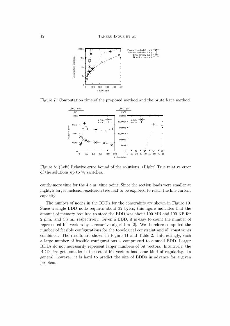
Figure 7 shows the computation time of our method and that of the brute force

method for networks of different sizes and two time points (2 p.m. and 4 a.m.).

Figure 8, left, plots the relative error bound (10) of our solutions. Our solution for

Loss Minimization of Power Distribution Networks with Guaranteed Error Bound 11

Table 1: Specification of the Fukui-TEPCO network.

Number of feeders 72Number of switches 468Number of sections 648Total load,

∑ni=1 Ii 287 MW at 2 p.m., and 113 MW at 4 a.m.

Line capacity, Jmax 300 ASending line voltage 6.6 kVMaximum voltage drop, Dmax 0.3 kV

Figure 6: Switch configuration of the Fukui-TEPCO network determined by ourmethod for the load profile at 4 a.m.

4 a.m. is partly visualized in Figure 6. Our method finished the whole optimization

procedure in less than three hours for the full network with 468 switches and the

relative error bound was 1.56% at most. As expected, the computational time of

the brute-force approach exploded quickly. With a time limit of 10,000 seconds,

the global optimal solution was obtained only up to 78 switches. Figure 8, right,

shows the true relative error of our solutions up to 78 switches. In many cases,

our solution was indeed optimal (i.e., the relative error was zero). The maximum

relative error was about 0.0225%; much smaller than the theoretical bound.

Figure 9 shows the computation time required by each process. The construc-

tion of BDDs for electrical constraints takes the largest fraction of the computation

time. This is because large inclusion-exclusion trees are produced without on-the-

fly merging, and computing voltage drop for each subgraph is time-consuming. In

contrast, the construction for the topological constraint finished in less than one

second even for up to 468 switches, clearly indicating the significant importance of

on-the-fly merging. The BDD construction for electrical constraints took signifi-

12 Takeru Inoue et al.

1

10

100

1000

10000

0 100 200 300 400 500

Com

puta

tion t

ime

[sec

.]

# of switches

Proposed method (2 p.m.)Proposed method (4 a.m.)

Brute force (2 p.m.)Brute force (4 a.m.)

Figure 7: Computation time of the proposed method and the brute force method.

0

0.005

0.01

0.015

0.02

0 100 200 300 400 500

Rel

ativ

e e

rror

# of switches

2 p.m.4 a.m.

0

5e-05

0.0001

0.00015

0.0002

0.00025

0.0003

0 10 20 30 40 50 60 70 80

2 p.m.4 a.m.

f(x*) - frelax

f(x*)

f(x*) - fopt

f(x*)

Figure 8: (Left) Relative error bound of the solutions. (Right) True relative errorof the solutions up to 78 switches.

cantly more time for the 4 a.m. time point; Since the section loads were smaller at

night, a larger inclusion-exclusion tree had to be explored to reach the line current

capacity.

The number of nodes in the BDDs for the constraints are shown in Figure 10.

Since a single BDD node requires about 32 bytes, this figure indicates that the

amount of memory required to store the BDD was about 100 MB and 100 KB for

2 p.m. and 4 a.m., respectively. Given a BDD, it is easy to count the number of

represented bit vectors by a recursive algorithm [2]. We therefore computed the

number of feasible configurations for the topological constraint and all constraints

combined. The results are shown in Figure 11 and Table 2. Interestingly, such

a large number of feasible configurations is compressed to a small BDD. Larger

BDDs do not necessarily represent larger numbers of bit vectors. Intuitively, the

BDD size gets smaller if the set of bit vectors has some kind of regularity. In

general, however, it is hard to predict the size of BDDs in advance for a given

problem.

Loss Minimization of Power Distribution Networks with Guaranteed Error Bound 13

0.01

0.1

1

10

100

1000

10000

0 100 200 300 400 500

Com

puta

tion

time

[sec

.]

# of switches

Topological constraintElectrical constraints

IntersectionComponent-level diagram

Shortest path search

0 100 200 300 400 500

2 p.m. 4 a.m.

Figure 9: Computation time of each process in the proposed method.

10

100

1000

10000

100000

1e+06

1e+07

0 100 200 300 400 500

BDD

size

# of switches

All constraints (2 p.m.)All constraints (4 a.m.)Topological constraint

Figure 10: BDD size for the constraints.

6 Conclusion

In this paper, we have developed an efficient network reconfiguration method that

yields an error bound. In the real-world settings, ad-hoc algorithms without solu-

tion quality guarantee are unlikely to be used because of the danger of returning

solutions incurring an excessive running cost for managing the network. It may be

possible to reduce the probability of such a catastrophic failure caused by local-

update-based methods, e.g. by using multiple starting points. However, since

distribution networks are fundamental infrastructure, failures cannot be allowed

even with the smallest probability. In contrast, our method is the first reliable

method with solution quality guarantee, hence we believe that this is an important

step towards automated network reconfiguration.

Acknowledgement

We would like to thank Takashi Horiyama, Takeaki Uno, Hirotaka Takano, Masakazu

Ishihata and David duVerle for their valuable comments.

14 Takeru Inoue et al.

1

1e+10

1e+20

1e+30

1e+40

1e+50

1e+60

1e+70

1e+80

0 100 200 300 400 500

# of

feas

ible

con

figur

atio

ns

# of switches

All constraints (2 p.m.)All constraints (4 a.m.)Topological constraint

Figure 11: Number of feasible configurations.

Table 2: Numbers of feasible configurations in a network of 468 switches.

Condition Number of feasible configurations BDD sizeAll constraints, loads at 2 p.m. 56549012847446003723757714431732193815091620755492933270200 3223985All constraints, loads at 4 a.m. 15052768726188994695810341375588783632354554002783638970270450179200000 3171Topological constraint 218646889093444243387855355581579747968214496454992053728787429330078125 1554

References

[1] M. Baran and F. Wu. Network reconfiguration in distribution systems for

loss reduction and load balancing. IEEE Transactions on Power Delivery,

4(2):1401–1407, 1989.

[2] R. Bryant. Graph-based algorithms for boolean function manipulation. IEEE

Transactions on Computers, C-35(8):677–691, 1986.

[3] E. Carreno, R. Romero, and A. Padilha-Feltrin. An efficient codification to

solve distribution network reconfiguration for loss reduction problem. IEEE

Transactions on Power Systems, 23(4):1542–1551, 2008.

[4] C. Cheng and D. Shirmohammadi. A three-phase power flow method for real-

time distribution system analysis. IEEE Transactions on Power Systems,

10(2):671–679, 1995.

[5] H.-D. Chiang and R. Jean-Jumeau. Optimal network reconfigurations in dis-

tribution systems. i. a new formulation and a solution methodology. IEEE

Transactions on Power Delivery, 5(4):1902–1909, 1990.

[6] S. Civanlar, J. Grainger, H. Yin, and S. Lee. Distribution feeder reconfigura-

tion for loss reduction. IEEE Transactions on Power Delivery, 3(3):1217–1223,

1988.

[7] O. Coudert. Solving graph optimization problems with ZBDDs. In Proceedings

of European Design and Test Conference, pages 224–228, 1997.

Loss Minimization of Power Distribution Networks with Guaranteed Error Bound 15

[8] B. Enacheanu, B. Raison, R. Caire, O. Devaux, W. Bienia, and N. HadjSaid.

Radial network reconfiguration using genetic algorithm based on the matroid

theory. IEEE Transactions on Power Systems, 23(1):186–195, 2008.

[9] Y. Hayashi, S. Kawasaki, J. Matsuki, H. Matsuda, S. Sakai, T. Miyazaki,

and N. Kobayashi. Establishment of a standard analytical model of distribu-

tion network with distributed generators and development of multi evaluation

method for network configuration candidates. IEEJ Transactions on Power

and Energy, 126(10):1013–1022, 2006. in Japanese.

[10] Y. Hayashi and J. Matsuki. Loss minimum configuration of distribution system

considering n-1 security of dispersed generators. IEEE Transactions on Power

Systems, 19(1):636–642, 2004.

[11] Y.-J. Jeon, J.-C. Kim, J.-O. Kim, J.-R. Shin, and K. Lee. An efficient simu-

lated annealing algorithm for network reconfiguration in large-scale distribu-

tion systems. IEEE Transactions on Power Delivery, 17(4):1070–1078, 2002.

[12] D. Knuth. The Art of Computer Programming, volume 4, Fascicle 1: Bitwise

Tricks and Techniques; Binary Decision Diagrams. Addison-Wesley, USA,

2009.

[13] W.-M. Lin and H.-C. Chin. A new approach for distribution feeder recon-

figuration for loss reduction and service restoration. IEEE Transactions on

Power Delivery, 13(3):870–875, 1998.

[14] T. McDermott, I. Drezga, and R. Broadwater. A heuristic nonlinear construc-

tive method for distribution system reconfiguration. IEEE Transactions on

Power Systems, 14(2):478–483, 1999.

[15] S. Minato. Zero-suppressed BDDs for set manipulation in combinatorial prob-

lems. In Proceedings of Conference on Design Automation, pages 272–277,

1993.

[16] A. Morton and I. Mareels. An efficient brute-force solution to the network

reconfiguration problem. IEEE Transactions on Power Delivery, 15(3):996–

1000, 2000.

[17] K. Nara, A. Shiose, M. Kitagawa, and T. Ishihara. Implementation of ge-

netic algorithm for distribution systems loss minimum re-configuration. IEEE

Transactions on Power Systems, 7(3):1044–1051, 1992.

[18] D. Shirmohammadi and H. Hong. Reconfiguration of electric distribution

networks for resistive line losses reduction. IEEE Transactions on Power

Delivery, 4(2):1492 –1498, 1989.