Technical Note Non-contact measurement of blade vibration

Technical Note

Non-contact measurement of blade vibrationin an axial compressor

Radoslaw Przysowa 1,∗ and Peter Russhard 2,

1 Instytut Techniczny Wojsk Lotniczych, ul. Ksiecia Bolesława 6, 01-494 Warszawa, Poland2 EMTD Ltd, 22 22 Woods Meadow, Derby, England, DE72 3UX, United Kingdom; [email protected]* Correspondence: [email protected]

Abstract: Complex blade responses such as a rotating stall or simultaneous resonances are common in modern engines and their observation can be a challenge even for state-of-the-art tip-timing systems and trained operators. This paper analyses forced vibrations of axial compressor blades, measured during the bench tests of the SO-3 turbojet. In relation to earlier studies conducted in ITWL with a small number of sensors, a multichannel tip-timing system let us observe simultaneous responses or higher-order modes. To find possible symptoms of a failure, blade responses in a healthy and unhealthy engine configuration with an inlet blocker were studied. The used analysis methods covered all-blade spectrum and the circumferential fitting o f b lade d eflections to th e harmonic oscillator model. The proposed modal solver can track the vibration frequency and adjust the engine order on the fly. That way, synchronous and asynchronous vibrations are observed and analysed together with an extended variant of least squares. The proposed approach helps to avoid common mistakes and saves a lot of work related to configuring the conventional solver.

Keywords: blade vibration; blade tip-timing; rotating stall; axial compressor; Blade Health Monitoring; least squares; bladed disc dynamics

1. Introduction

Non-contact blade vibration measurement, known as Blade Tip-Timing (BTT) or Non-contactStress Measurement System (NSMS), is a technique for determining dynamic blade stresses to ensurethe structural integrity of bladed disks in jet engines and stationary turbines [1,2]. It can be used inaxial or radial compressors [3] and unshrouded or shrouded turbines [4]. The method uses severalsensors mounted circumferentially to precisely determine temporary positions of each blade tip inevery rotation [5]. Model-based data processing is necessary to determine the real amplitude andvibration [6,7]. BTT solutions used by industry are still based on algorithms established at the endof the 20th century. Most vibration surveys rely upon traversing each of the resonances. Analysingresponses at a constant speed is more difficult to achieve.

In most applications, undersampled tip deflection signals are generally processed by the twogroups of methods: 1) Fourier spectral analysis, e.g. all-blade spectrum, 2) Least Squares Fitting(LSF). Fourier transform methods compromise time and frequency resolution and involve significantpost-processing to reconstruct the real spectrum. They are now used primarily to identify the presenceof non-integral vibration and to determine nominal frequency and nodal diameter. This data seedsleast squares fitting [8]. LSF is now the main method used in most of BTT systems to extract the realamplitude and phase for successive revolutions. It can be used either circumferentially to fit the blademode or axially to fit the mode shape - each has a different strategy for conversion to stress [9]. Themodels for this can be simplistic sine fitting [10] or more complex ones derived from the Finite ElementMethod (FEM) during the calibration and validation process used with BTT.

Alternative methods introduced in the previous decade such as auto-regressive [11], spectralestimation using nonuniform sampling [12] or full-signal analysis using many points per blade pass

Preprints (www.preprints.org) | NOT PEER-REVIEWED | Posted: 24 November 2019 doi:10.20944/preprints201911.0279.v1

© 2019 by the author(s). Distributed under a Creative Commons CC BY license.

Peer-reviewed version available at Sensors 2019, 20, 68; doi:10.3390/s20010068

https://orcid.org/0000-0001-9649-0179

https://orcid.org/0000-0002-3965-4234

https://doi.org/10.20944/preprints201911.0279.v1

http://creativecommons.org/licenses/by/4.0/

https://doi.org/10.3390/s20010068

2 of 16

[13], were too complex or not efficient enough to leave the labs and be widely used by the community.These alternative methods provide little additional capability to the BTT technology but are oftenrevisited by researchers [14–16] in the hope of finding methods for in-service Blade Health Monitoring(BHM), where the blade sets are already well understood.

A significant number of papers, introducing new BTT models and algorithms such as a newtwo-parameter plot method [17], convolutional neural networks [18], aliasing reduction [19,20], sparserepresentation and compressed sensing [21] were published recently, but they can be applied in reallife to a limited extent. Several newly introduced algorithms work well only with simulated or rigacquired data, usually with a single response of the first mode. Further efforts are needed to makethem more mature to better deal with noise and weak or more complex responses.

Validation against simulation is not accepted for certification of engines [22]. BTT technique wasalready used in component certification tests, where the evidence to calculate a meaningful value ofstress was produced [23]. However, a documented validation of the measurement system and abilityto estimate uncertainty are still missing in many BTT applications.

2. Materials and Methods

The conducted engine tests were aimed to characterise blade vibrations i.e. identify existingresponses, especially high-order ones. This is often necessary when investigating blade failure inlegacy compressors or turbines, when design data are not available or not reliable.

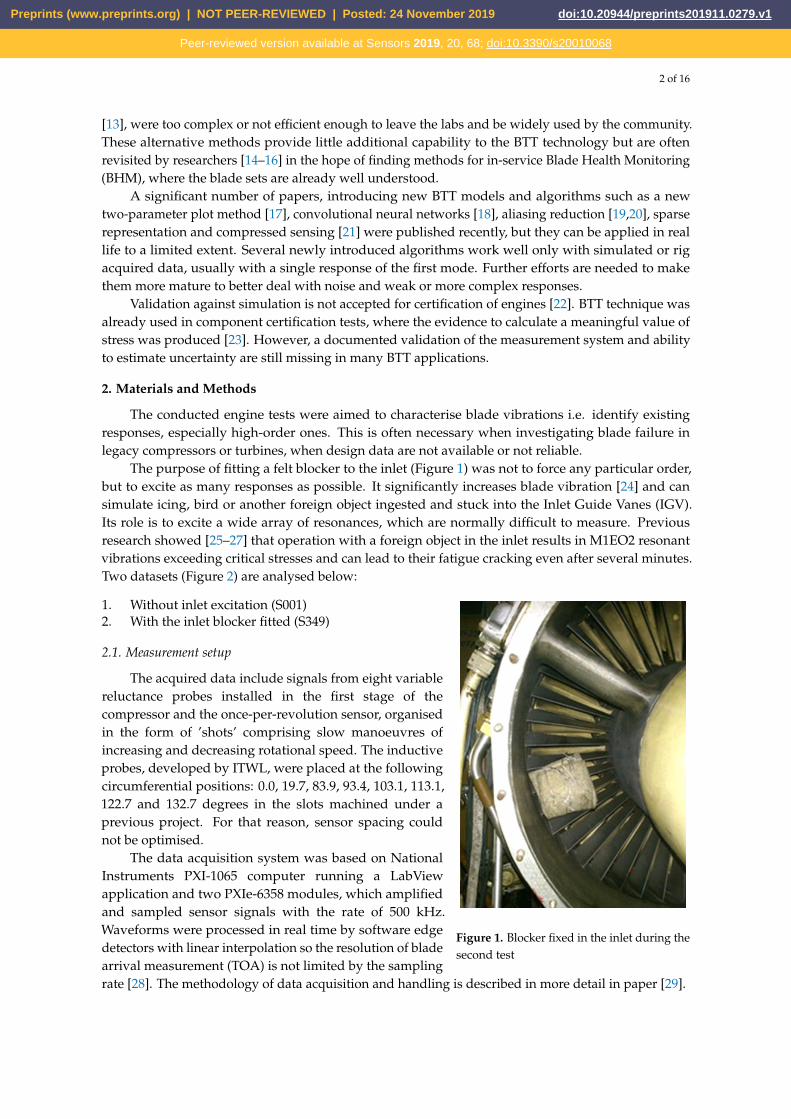
The purpose of fitting a felt blocker to the inlet (Figure 1) was not to force any particular order,but to excite as many responses as possible. It significantly increases blade vibration [24] and cansimulate icing, bird or another foreign object ingested and stuck into the Inlet Guide Vanes (IGV).Its role is to excite a wide array of resonances, which are normally difficult to measure. Previousresearch showed [25–27] that operation with a foreign object in the inlet results in M1EO2 resonantvibrations exceeding critical stresses and can lead to their fatigue cracking even after several minutes.

Figure 1. Blocker fixed in the inlet during thesecond test

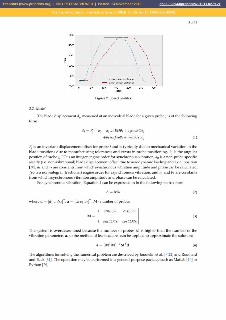
Two datasets (Figure 2) are analysed below:

1. Without inlet excitation (S001)2. With the inlet blocker fitted (S349)

2.1. Measurement setup

The acquired data include signals from eight variablereluctance probes installed in the first stage of thecompressor and the once-per-revolution sensor, organisedin the form of ’shots’ comprising slow manoeuvres ofincreasing and decreasing rotational speed. The inductiveprobes, developed by ITWL, were placed at the followingcircumferential positions: 0.0, 19.7, 83.9, 93.4, 103.1, 113.1,122.7 and 132.7 degrees in the slots machined under aprevious project. For that reason, sensor spacing couldnot be optimised.

The data acquisition system was based on NationalInstruments PXI-1065 computer running a LabViewapplication and two PXIe-6358 modules, which amplifiedand sampled sensor signals with the rate of 500 kHz.Waveforms were processed in real time by software edgedetectors with linear interpolation so the resolution of bladearrival measurement (TOA) is not limited by the samplingrate [28]. The methodology of data acquisition and handling is described in more detail in paper [29].




https://doi.org/10.3390/s20010068

3 of 16

Figure 2. Speed profiles

2.2. Model

The blade displacement dj, measured at an individual blade for a given probe j is of the followingform:

dj = Pj + a0 + a1sinEOθj + a2cosEOθj

+b1sin f eoθj + b2cos f eoθj (1)

Pj is an invariant displacement offset for probe j and is typically due to mechanical variation in theblade positions due to manufacturing tolerances and errors in probe positioning. θj is the angularposition of probe j; EO is an integer engine order for synchronous vibration; a0 is a non-probe specific,steady (i.e. non-vibrational) blade displacement offset due to aerodynamic loading and axial position[30], a1 and a2 are constants from which synchronous vibration amplitude and phase can be calculated;f eo is a non-integral (fractional) engine order for asynchronous vibration; and b1 and b2 are constantsfrom which asynchronous vibration amplitude and phase can be calculated.

For synchronous vibration, Equation 1 can be expressed in in the following matrix form:

d = Ma (2)

where d = [d1 .. dM]T , a = [a0 a1 a2]T , M - number of probes

M =

∣∣∣∣∣∣∣1 sinEOθ1 cosEOθ1

..1 sinEOθM cosEOθM

∣∣∣∣∣∣∣ (3)

The system is overdetermined because the number of probes M is higher then the number of thevibration parameters a, so the method of least squares can be applied to approximate the solution:

a = (MTM)−1MTd. (4)

The algorithms for solving the numerical problem are described by Jousselin et al. [7,22] and Russhardand Back [31]. The operation may be performed in a general-purpose package such as Matlab [10] orPython [29].




https://doi.org/10.3390/s20010068

4 of 16

The obtained vector a is substituted to Equation 2 to compare the calculated displacements d withthe measured ones d. It is more convenient to use correlation between d and d to evaluate the goodnessof fit instead of the residual d − d. The correlation coefficient r is calculated using the Pearson formula:

r = ∑(d − d)(d − d)√∑(d − d)2(d − d)2

(5)

This parameter ranges from 0 to 1 and is called ’coherence’ below.

2.3. Stack pattern

From Equation 1 it can be seen that for a blade undergoing no vibration, its steady statedisplacement is equal to Pj. For an ideal rotor with equally spaced blades, the value for each bladewould be identical. In reality, the difference in manufacturing tolerances produces a pattern ofdisplacements, which are the differences from the ideal position. It is unique for each rotor and shownas the stack plot [7]. It is calculated for each probe j by averaging blade displacements over manyrevolutions:

Pij =1H

H

∑h=1

dhij (6)

h is the revolution number, i - the blade number, H - the number of revolutions.Changes in the stack pattern occur if (a) the blades undergo vibration [32] or (b) if the rotor

is permanently damaged for some reasons. The stack plot is used to verify that the collected datasets were aligned correctly and is often applied as the first level of data validation. The analysis ofmisaligned data is a common fault in BTT data analysis.

2.4. Software

Blade deflection signals include undesirable components, such as noise, a static offset, a lineartrend, and also some asynchronous vibration, which is not of interest. Conventional processing of BTTdata relies upon preliminary operations such as alignment to ensure all data comes from the samerotation number, zeroing to isolate Pj and filtering to isolate the integral response from the non-integralresponse [33].

In practice, the number of resonances, blades and probes to analyse is sufficiently large thatpre-processing and resonance fitting must be automated. The automation of analysis was achievedby Rolls-Royce, which developed their Batch Processor software [34], which was released severalyears ago. The solver separates the integral and non-integral components of the blade displacementand uses a form of least squares fitting to generate the results for integral and non-integral responses.Where integral and non-integral displacements precede and follow on an integral response, or occursimultaneously, then that software fails.

In this work, a new solver called EMTD Multitool [35] is used. It has the ability to operateconventionally or by using alternative methods of pre-processing the data, which can be manipulatedinto the form:

dj = a0 + a1sinEOθj + a2cosEOθj (7)

where the value of EO is real number rather than an integer.

2.5. Uncertainty measurement

BTT uncertainties can be divided into three categories: those inherent in the physical act of takingthe measurement, the pre-processing of the acquired data including the conversion to deflection andfrequency, and finally, the challenge of converting the obtained deflections into blade stress [36]. Thecurrent capability of BTT for use in a compressor stress survey can, if all of the above uncertainties




https://doi.org/10.3390/s20010068

5 of 16

are addressed and controlled, produce end-to-end stress measurement with uncertainties of ±2.5% orbetter. More importantly, a figure of uncertainty can now be calculated for every BTT measurement.

Typically, BTT responses are characterised by the quality of the least squares fitting. However,measurement uncertainty is often not known and the decision on whether the results are ‘good’ issubject to opinion. The calculation of the uncertainty value removes this doubt and provides upperand lower values to any BTT measurement.

The MultiTool solver calculates the measurement uncertainty for any point on the tracked orderresponse. To do this, the least squares model is extended to contain a term that ‘captures’ any datathat does not correlate with the engine order term. The uncertainty term includes the average andstandard deviation of the non-related terms. From this, the measurement uncertainty is calculated overa pre-determined number of revolutions. The form of unc is not disclosed in this paper for commercialreasons.

dj = a0 + unc + a1sinEOθj + a2cosEOθj (8)

2.6. Data analysis

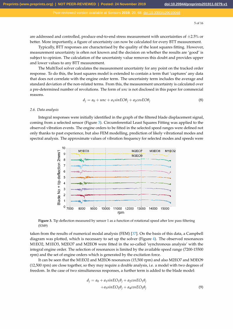
Integral responses were initially identified in the graph of the filtered blade displacement signal,coming from a selected sensor (Figure 3). Circumferential Least Squares Fitting was applied to theobserved vibration events. The engine orders to be fitted in the selected speed ranges were defined notonly thanks to past experience, but also FEM modelling, prediction of likely vibrational modes andspectral analysis. The approximate values of vibration frequency for selected modes and speeds were

Figure 3. Tip deflection measured by sensor 1 as a function of rotational speed after low pass filtering(S349)

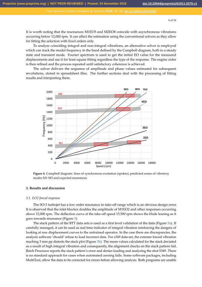
taken from the results of numerical modal analysis (FEM) [37]. On the basis of this data, a Campbelldiagram was plotted, which is necessary to set up the solver (Figure 4). The observed resonancesM1EO2, M1EO3, M2EO7 and M2EO8 were fitted in the so-called ’synchronous analysis’ with theintegral engine order. The selection of resonances is limited by the available speed range (7200-15500rpm) and the set of engine orders which is generated by the excitation force.

It can be seen that the M1EO2 and M2EO6 resonances (15,500 rpm) and also M2EO7 and M3EO9(12,500 rpm) are close together, so they may require a double analysis, i.e. a model with two degrees offreedom. In the case of two simultaneous responses, a further term is added to the blade model:

dj = a0 + a1sinEO1θj + a2cosEO1θj

+a3sinEO2θj + a4cosEO2θj (9)




https://doi.org/10.3390/s20010068

6 of 16

It is worth noting that the resonances M1EO3 and M2EO8 coincide with asynchronous vibrationsoccurring below 12,000 rpm. It can affect the estimation using the conventional solvers as they allowfor fitting the selection with fixed orders only.

To analyse coinciding integral and non-integral vibrations, an alternative solver is employedwhich can track the modal frequency in the band defined by the Campbell diagram, both in a steadystate and transient mode. Fourier spectrum is used to get the initial EO value for the measureddisplacements and use it for least square fitting regardless the type of the response. The engine orderis then refined and the process repeated until satisfactory coherence is achieved.

The solver delivers the sequence of amplitude and phase values estimated for subsequentrevolutions, stored in spreadsheet files. The further sections deal with the processing of fittingresults and interpreting them.

0

200

400

600

800

1000

1200

1400

1600

1800

2000

0 2000 4000 6000 8000 10000 12000 14000 16000 18000

Freq

uenc

y (H

z)

Speed (rpm)

7EO8EO9EO

6EO

3EO

2EO

M1

M2

M3

Figure 4. Campbell diagram: lines of synchronous excitation (spokes), predicted zones of vibratorymodes M1-M3 and expected resonances

3. Results and discussion

3.1. EO2 forced response

The SO-3 turbojet has a low order resonance in take-off range which is an obvious design error.It is observed that the inlet blocker doubles the amplitude of M1EO2 and other responses occurringabove 12,000 rpm. The deflection curve at the take-off speed 15,500 rpm shows the blade leaning as itgoes towards resonance (Figure 3).

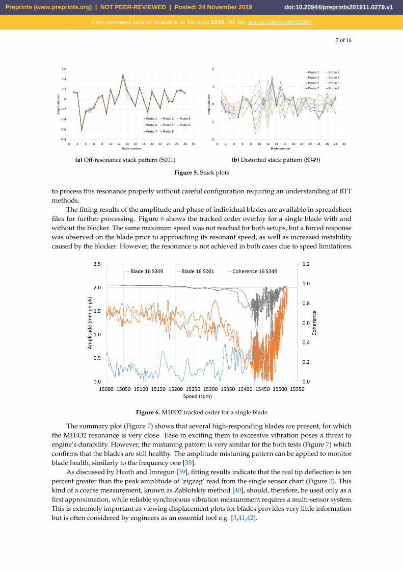
The stack pattern of the BTT data sets is used as a first level validation of the data (Figure 5a). Ifcarefully managed, it can be used as real time indicator of integral vibration reinforcing the dangers oflooking at raw displacement curves to the untrained operator. In the case there are discrepancies, theanalysis software ’should’ refuse to load incorrect data. For s349 data-set, the extreme forced vibrationreaching 3 mm pp distorts the stack plot (Figure 5b). The mean values calculated for the stack deviatedas a result of high integral vibration and consequently, the alignment checks on the stack pattern fail.Batch Processor reports the stack pattern’s error and denies loading and analysing the shot S349. Thereis no standard approach for cases when automated zeroing fails. Some software packages, includingMultiTool, allow the data to be corrected for errors before allowing analysis. Both programs are unable




https://doi.org/10.3390/s20010068

7 of 16

-0.8

-0.6

-0.4

-0.2

0

0.2

0.4

0.6

0 2 4 6 8 10 12 14 16 18 20 22 24 26 28 30

Ampl

itude

mm

Blade number

Probe 1 Probe 2 Probe 3

Probe 4 Probe 5 Probe 6

Probe 7 Probe 8

(a) Off-resonance stack pattern (S001)

-2

-1

0

1

2

0 2 4 6 8 10 12 14 16 18 20 22 24 26 28 30

Ampl

itude

mm

Blade number

Probe 1 Probe 2

Probe 3 Probe 4

Probe 5 Probe 6

Probe 7 Probe 8

(b) Distorted stack pattern (S349)

Figure 5. Stack plots

to process this resonance properly without careful configuration requiring an understanding of BTTmethods.

The fitting results of the amplitude and phase of individual blades are available in spreadsheetfiles for further processing. Figure 6 shows the tracked order overlay for a single blade with andwithout the blocker. The same maximum speed was not reached for both setups, but a forced responsewas observed on the blade prior to approaching its resonant speed, as well as increased instabilitycaused by the blocker. However, the resonance is not achieved in both cases due to speed limitations.

Figure 6. M1EO2 tracked order for a single blade

The summary plot (Figure 7) shows that several high-responding blades are present, for whichthe M1EO2 resonance is very close. Ease in exciting them to excessive vibration poses a threat toengine’s durability. However, the mistuning pattern is very similar for the both tests (Figure 7) whichconfirms that the blades are still healthy. The amplitude mistuning pattern can be applied to monitorblade health, similarly to the frequency one [38].

As discussed by Heath and Imregun [39], fitting results indicate that the real tip deflection is tenpercent greater than the peak amplitude of ’zigzag’ read from the single sensor chart (Figure 3). Thiskind of a coarse measurement, known as Zablotskiy method [40], should, therefore, be used only as afirst approximation, while reliable synchronous vibration measurement requires a multi-sensor system.This is extremely important as viewing displacement plots for blades provides very little informationbut is often considered by engineers as an essential tool e.g. [3,41,42].




https://doi.org/10.3390/s20010068

8 of 16

2 4 6 8 10 12 14 16 18 20 22 24 26 28Blades

0.0

0.5

1.0

1.5

2.0

2.5

Ampl

itude

(mm

pk-

pk)

With blockersWithout blockers

Figure 7. M1EO2 peak amplitude response for all blades

3.2. Frequency estimation

In theory, vibration phase changes the sign when crossing the resonance but a 180-degree phaseshift is observed in rare cases and cannot be used reliably to confirm the location of resonances. Ina real test environment, examining each phase response visually is impractical even for low-orderresponses, which need many revolutions to sweep. If the phase shift was used as the only indicatordefining the resonance, then less than 1% of existing resonances would be found in real engine datasets.

Mostly, it is assumed that the blade resonant frequency occurs at the point where amplitudereaches a maximum value. The quality factor of metal blades is high (e.g. 200 or more) so the resonancepeak is a good approximation of the resonant frequency. The frequency measurements presentedin the next section are obtained in this way. Unfortunately, the M1EO2 resonance is located in thevicinity of the upper-speed limit. As a result, no phase transition by zero is observed for the majority ofblades, which means that the resonant frequency was not achieved and cannot be reliably determined.Therefore, the values presented in Figure 7 correspond to the maximum amplitude reached by thesolver.

In the case when full resonance is not achieved, erroneous results can be produced, although thisis the same as with strain gauges. For M1EO2, checking the phase shift helps to avoid presenting falsefrequencies. In other cases, it is usually not necessary and could remove potentially good data, if thethreshold is increased over 105 degrees. There is no simple method of obtaining the running frequencyof the blades where the M1EO2 resonance is located beyond the maximum speed. The solution is toincrease the maximum engine speed but it is not recommended.

3.3. Higher order resonances

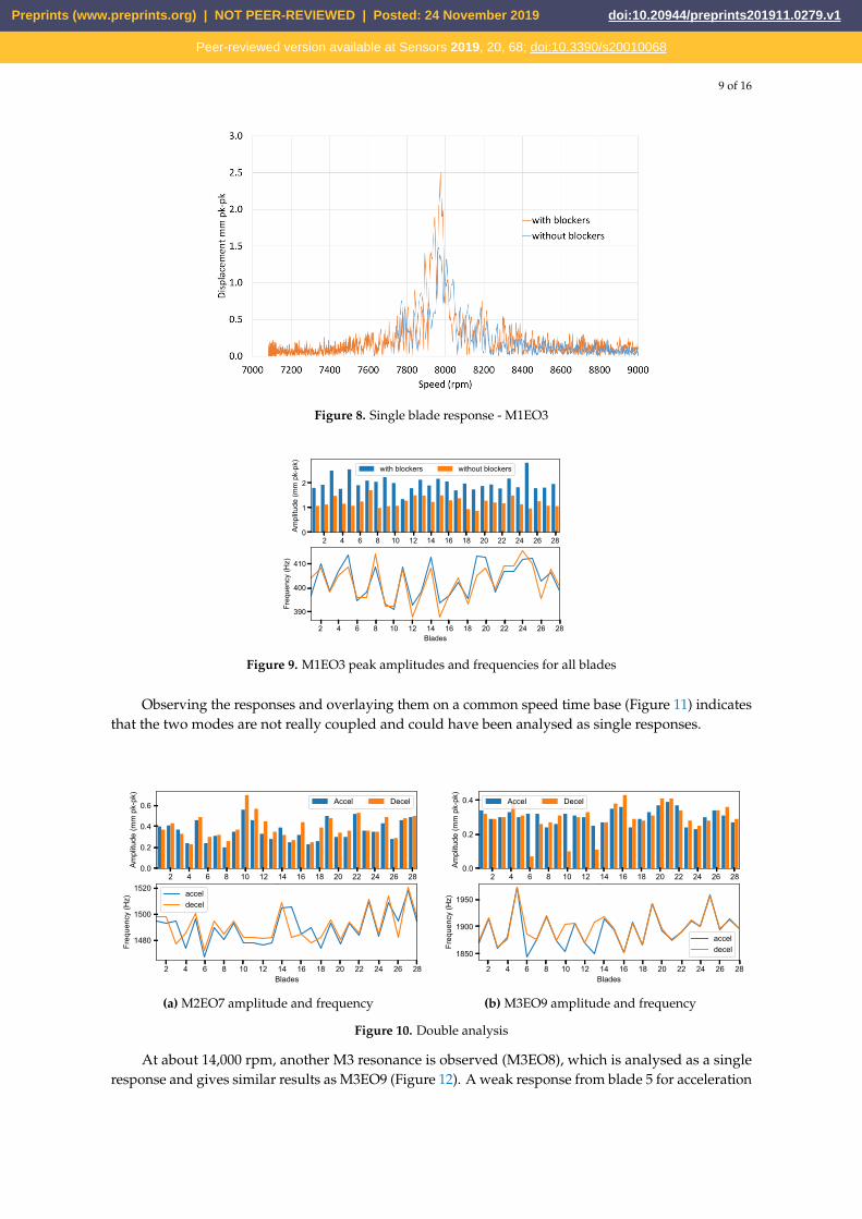
The increase in amplitude caused by the blocker is also observed for the M1EO3 crossing at 8,000rpm (Figure 8). The tracked order blade response shows the increase and decay of the amplitude.The resonance is traversed during the engine manoeuvre, so the blade response frequencies can becompared (Figure 9). The uncertainty of the presented resonant amplitudes is limited to 5% and isaround 1% for the majority of blades. Therefore, error bars are not displayed in summary plots to avoidblurring them. The blade amplitudes of the other resonances predicted by the Campbell diagram canbe also extracted. It turns out that integral M2 and M3 vibrations respond well only when the blockeris installed (shot s349). Figure 10a shows M2EO7 observed at 12,800 rpm which may be coincidentwith M3EO9, thus it is calculated as a double response. Similarly, the results from the double analysisfor M3EO9 are shown in Figure 10b. This method involves factorisation of a larger matrix and thustakes significantly more time than the single analysis.




https://doi.org/10.3390/s20010068

9 of 16

Figure 8. Single blade response - M1EO3

2 4 6 8 10 12 14 16 18 20 22 24 26 28Blades

0

1

2

Ampl

itude

(mm

pk-

pk)

with blockers without blockers

2 4 6 8 10 12 14 16 18 20 22 24 26 28Blades

390

400

410

Freq

uenc

y (H

z)

Figure 9. M1EO3 peak amplitudes and frequencies for all blades

Observing the responses and overlaying them on a common speed time base (Figure 11) indicatesthat the two modes are not really coupled and could have been analysed as single responses.

2 4 6 8 10 12 14 16 18 20 22 24 26 28Blades

0.0

0.2

0.4

0.6

Ampl

itude

(mm

pk-

pk)

Accel Decel

2 4 6 8 10 12 14 16 18 20 22 24 26 28Blades

1480

1500

1520

Freq

uenc

y (H

z)

acceldecel

(a) M2EO7 amplitude and frequency

2 4 6 8 10 12 14 16 18 20 22 24 26 28Blades

0.0

0.2

0.4

Ampl

itude

(mm

pk-

pk)

Accel Decel

2 4 6 8 10 12 14 16 18 20 22 24 26 28Blades

1850

1900

1950

Freq

uenc

y (H

z)

acceldecel

(b) M3EO9 amplitude and frequency

Figure 10. Double analysis

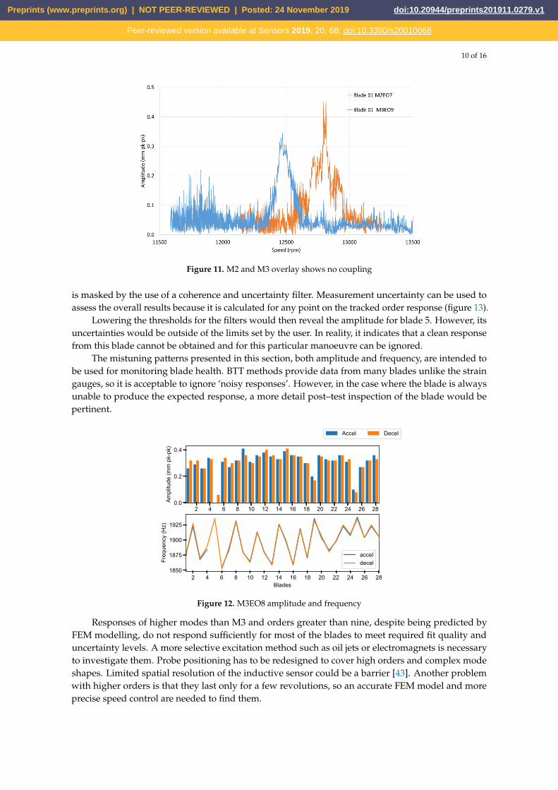
At about 14,000 rpm, another M3 resonance is observed (M3EO8), which is analysed as a singleresponse and gives similar results as M3EO9 (Figure 12). A weak response from blade 5 for acceleration




https://doi.org/10.3390/s20010068

10 of 16

Figure 11. M2 and M3 overlay shows no coupling

is masked by the use of a coherence and uncertainty filter. Measurement uncertainty can be used toassess the overall results because it is calculated for any point on the tracked order response (figure 13).

Lowering the thresholds for the filters would then reveal the amplitude for blade 5. However, itsuncertainties would be outside of the limits set by the user. In reality, it indicates that a clean responsefrom this blade cannot be obtained and for this particular manoeuvre can be ignored.

The mistuning patterns presented in this section, both amplitude and frequency, are intended tobe used for monitoring blade health. BTT methods provide data from many blades unlike the straingauges, so it is acceptable to ignore ‘noisy responses’. However, in the case where the blade is alwaysunable to produce the expected response, a more detail post–test inspection of the blade would bepertinent.

2 4 6 8 10 12 14 16 18 20 22 24 26 28Blades

0.0

0.2

0.4

Ampl

itude

(mm

pk-

pk)

2 4 6 8 10 12 14 16 18 20 22 24 26 28Blades

1850

1875

1900

1925

Freq

uenc

y (H

z)

acceldecel

Accel Decel

Figure 12. M3EO8 amplitude and frequency

Responses of higher modes than M3 and orders greater than nine, despite being predicted byFEM modelling, do not respond sufficiently for most of the blades to meet required fit quality anduncertainty levels. A more selective excitation method such as oil jets or electromagnets is necessaryto investigate them. Probe positioning has to be redesigned to cover high orders and complex modeshapes. Limited spatial resolution of the inductive sensor could be a barrier [43]. Another problemwith higher orders is that they last only for a few revolutions, so an accurate FEM model and moreprecise speed control are needed to find them.




https://doi.org/10.3390/s20010068

11 of 16

Figure 13. M3EO8 amplitude uncertainty

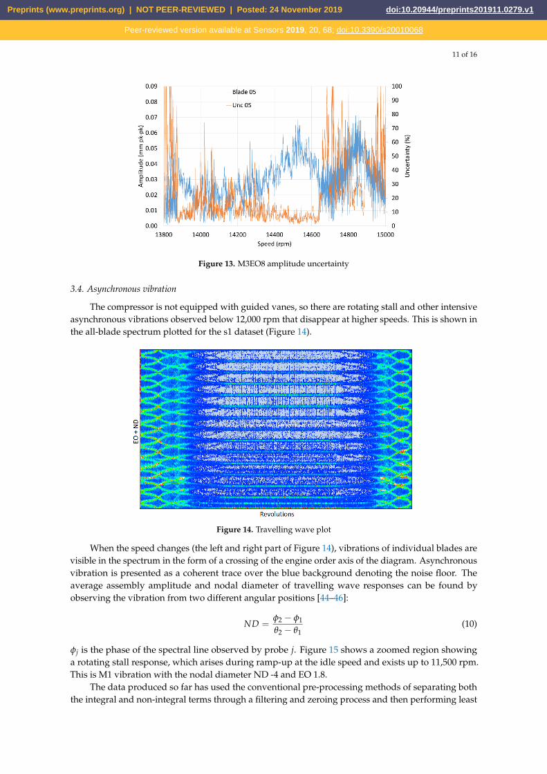
3.4. Asynchronous vibration

The compressor is not equipped with guided vanes, so there are rotating stall and other intensiveasynchronous vibrations observed below 12,000 rpm that disappear at higher speeds. This is shown inthe all-blade spectrum plotted for the s1 dataset (Figure 14).

Figure 14. Travelling wave plot

When the speed changes (the left and right part of Figure 14), vibrations of individual blades arevisible in the spectrum in the form of a crossing of the engine order axis of the diagram. Asynchronousvibration is presented as a coherent trace over the blue background denoting the noise floor. Theaverage assembly amplitude and nodal diameter of travelling wave responses can be found byobserving the vibration from two different angular positions [44–46]:

ND =φ2 − φ1

θ2 − θ1(10)

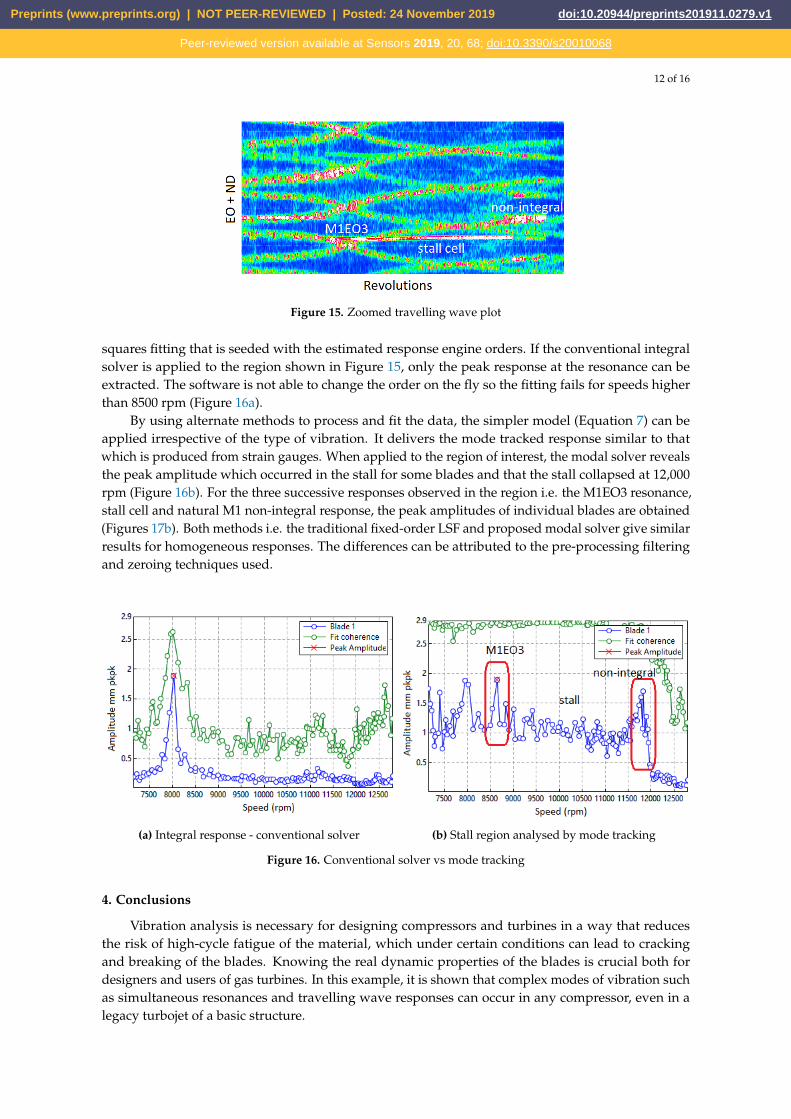
φj is the phase of the spectral line observed by probe j. Figure 15 shows a zoomed region showinga rotating stall response, which arises during ramp-up at the idle speed and exists up to 11,500 rpm.This is M1 vibration with the nodal diameter ND -4 and EO 1.8.

The data produced so far has used the conventional pre-processing methods of separating boththe integral and non-integral terms through a filtering and zeroing process and then performing least




https://doi.org/10.3390/s20010068

12 of 16

Figure 15. Zoomed travelling wave plot

squares fitting that is seeded with the estimated response engine orders. If the conventional integralsolver is applied to the region shown in Figure 15, only the peak response at the resonance can beextracted. The software is not able to change the order on the fly so the fitting fails for speeds higherthan 8500 rpm (Figure 16a).

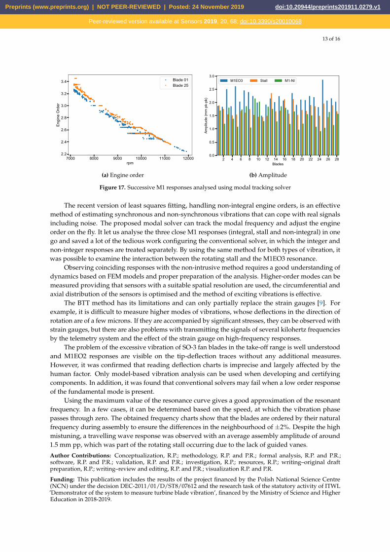
By using alternate methods to process and fit the data, the simpler model (Equation 7) can beapplied irrespective of the type of vibration. It delivers the mode tracked response similar to thatwhich is produced from strain gauges. When applied to the region of interest, the modal solver revealsthe peak amplitude which occurred in the stall for some blades and that the stall collapsed at 12,000rpm (Figure 16b). For the three successive responses observed in the region i.e. the M1EO3 resonance,stall cell and natural M1 non-integral response, the peak amplitudes of individual blades are obtained(Figures 17b). Both methods i.e. the traditional fixed-order LSF and proposed modal solver give similarresults for homogeneous responses. The differences can be attributed to the pre-processing filteringand zeroing techniques used.

(a) Integral response - conventional solver (b) Stall region analysed by mode tracking

Figure 16. Conventional solver vs mode tracking

4. Conclusions

Vibration analysis is necessary for designing compressors and turbines in a way that reducesthe risk of high-cycle fatigue of the material, which under certain conditions can lead to crackingand breaking of the blades. Knowing the real dynamic properties of the blades is crucial both fordesigners and users of gas turbines. In this example, it is shown that complex modes of vibration suchas simultaneous resonances and travelling wave responses can occur in any compressor, even in alegacy turbojet of a basic structure.




https://doi.org/10.3390/s20010068

13 of 16

7000 8000 9000 10000 11000 12000rpm

2.2

2.4

2.6

2.8

3.0

3.2

3.4

Engi

ne O

rder

Blade 01Blade 25

(a) Engine order

2 4 6 8 10 12 14 16 18 20 22 24 26 28Blades

0.0

0.5

1.0

1.5

2.0

2.5

3.0

Ampl

itude

(mm

pk-

pk)

M1EO3 Stall M1-NI

(b) Amplitude

Figure 17. Successive M1 responses analysed using modal tracking solver

The recent version of least squares fitting, handling non-integral engine orders, is an effectivemethod of estimating synchronous and non-synchronous vibrations that can cope with real signalsincluding noise. The proposed modal solver can track the modal frequency and adjust the engineorder on the fly. It let us analyse the three close M1 responses (integral, stall and non-integral) in onego and saved a lot of the tedious work configuring the conventional solver, in which the integer andnon-integer responses are treated separately. By using the same method for both types of vibration, itwas possible to examine the interaction between the rotating stall and the M1EO3 resonance.

Observing coinciding responses with the non-intrusive method requires a good understanding ofdynamics based on FEM models and proper preparation of the analysis. Higher-order modes can bemeasured providing that sensors with a suitable spatial resolution are used, the circumferential andaxial distribution of the sensors is optimised and the method of exciting vibrations is effective.

The BTT method has its limitations and can only partially replace the strain gauges [9]. Forexample, it is difficult to measure higher modes of vibrations, whose deflections in the direction ofrotation are of a few microns. If they are accompanied by significant stresses, they can be observed withstrain gauges, but there are also problems with transmitting the signals of several kilohertz frequenciesby the telemetry system and the effect of the strain gauge on high-frequency responses.

The problem of the excessive vibration of SO-3 fan blades in the take-off range is well understoodand M1EO2 responses are visible on the tip-deflection traces without any additional measures.However, it was confirmed that reading deflection charts is imprecise and largely affected by thehuman factor. Only model-based vibration analysis can be used when developing and certifyingcomponents. In addition, it was found that conventional solvers may fail when a low order responseof the fundamental mode is present.

Using the maximum value of the resonance curve gives a good approximation of the resonantfrequency. In a few cases, it can be determined based on the speed, at which the vibration phasepasses through zero. The obtained frequency charts show that the blades are ordered by their naturalfrequency during assembly to ensure the differences in the neighbourhood of ±2%. Despite the highmistuning, a travelling wave response was observed with an average assembly amplitude of around1.5 mm pp, which was part of the rotating stall occurring due to the lack of guided vanes.

Author Contributions: Conceptualization, R.P.; methodology, R.P. and P.R.; formal analysis, R.P. and P.R.;software, R.P. and P.R.; validation, R.P. and P.R.; investigation, R.P.; resources, R.P.; writing–original draftpreparation, R.P.; writing–review and editing, R.P. and P.R.; visualization R.P. and P.R.

Funding: This publication includes the results of the project financed by the Polish National Science Centre(NCN) under the decision DEC-2011/01/D/ST8/07612 and the research task of the statutory activity of ITWL’Demonstrator of the system to measure turbine blade vibration’, financed by the Ministry of Science and HigherEducation in 2018-2019.




https://doi.org/10.3390/s20010068

14 of 16

Acknowledgments: We would like to thank Michał Wachłaczenko and Wojciech Sujka for their involvement inthe project and support for engine tests.

Conflicts of Interest: The authors declare no conflict of interest.

Abbreviations

The following symols and abbreviations are used in this manuscript:φj phase observed by probe jθj angular position of probe jdj blade displacement measured by probe jH number of revolutionsh revolution numberi blade numberj probe numberN number of bladesM number of probesPj invariant offset for probe junc uncertaintyBHM Blade Health MonitoringBTT Blade Tip-TimingEO Engine OrderFEM Finite Element Methodf eo fractional engine orderFFT Fast Fourier TransformIGV Inlet Guide VanesITWL Air Force Institute of Technology in WarsawLSF Least Squares FittingM1 1st vibration modeMDPI Multidisciplinary Digital Publishing InstituteND nodal diameterNI non-integral vibrationsNSMS Non-contact Stress Measurement Systempk-pk peak-to-peak amplituder correlation / coherenceRMS Root Mean Squarerpm revolutions per minute

References

1. Russhard, P. The Rise and Fall of the Rotor Blade Strain Gauge. In Vibration Engineering and Technology ofMachinery; Sinha, J.K., Ed.; Springer International Publishing: Cham, 2015; Vol. 23, Mechanisms and MachineScience, pp. 27–38. doi:10.1007/978-3-319-09918-7.

2. Mevissen, F.; Meo, M. A Review of NDT/Structural Health Monitoring Techniques for Hot GasComponents in Gas Turbines. Sensors 2019, 19, 711. doi:10.3390/s19030711.

3. Zhao, X.; Zhou, Q.; Yang, S.; Li, H. Rotating Stall Induced Non-Synchronous Blade. Sensors (Switzerland)2019, 19. doi:10.3390/s19224995.

4. Ye, D.; Duan, F.; Jiang, J.; Cheng, Z.; Niu, G.; Shan, P.; Zhang, J. Synchronous vibration measurements forshrouded blades based on fiber optical sensors with lenses in a steam turbine. Sensors (Switzerland) 2019,19. doi:10.3390/s19112501.

5. Agilis Non-Intrusive Stress Measurement Systems Fundamentals. Technical report, Agilis MeasurementSystems, 2014.

6. Tappert, P.; Losh, D. Analyze Blade Vibration 6.1 User Manual. Technical Report October, Hood TechnologyCorporation, 2007.

7. Jousselin, O. Development of Blade Tip Timing Techniques in Turbo Machinery. PhD thesis, Manchester,2013.



https://doi.org/10.1007/978-3-319-09918-7

https://doi.org/10.3390/s19030711

https://doi.org/10.3390/s19224995

https://doi.org/10.3390/s19112501


https://doi.org/10.3390/s20010068

15 of 16

8. Russhard, P. Analysis of Rotating Stall in a Contra-Rotating System using Blade Tip Timing. Proceedingsof the 58th International Instrumentation Symposium; The International Society of Automation: San Diego,2012; pp. 1–33.

9. Knappett, D.; Garcia, J. Blade tip timing and strain gauge correlation on compressor blades. Proceedingsof the Institution of Mechanical Engineers, Part G: Journal of Aerospace Engineering 2008, 222, 497–506.doi:10.1243/09544100JAERO257.

10. Przysowa, R. The Analysis Of Synchronous Blade Vibration Using Linear Sine Fitting. Journal of KONBiN2014, 30, 5–19. doi:10.2478/jok-2014-0011.

11. Dimitriadis, G.; Carrington, I.; Wright, J.; Cooper, J. Blade-Tip Timing measurement of SynchronousVibrations of Rotating Blade assemblies. Mechanical Systems and Signal Processing 2002, 16, 599–622.doi:10.1006/mssp.2002.1489.

12. Beauseroy, P.; Lengellé, R. Nonintrusive turbomachine blade vibration measurement system. MechanicalSystems and Signal Processing 2007, 21, 1717–1738. doi:10.1016/j.ymssp.2006.07.015.

13. Teolis, C.; Teolis, A.; Paduano, J.; Lackner, M. Analytic representation of eddy current sensor data for faultdiagnostics. IEEE Aerospace Conference Proceedings 2005, 2005, 1–11. doi:10.1109/AERO.2005.1559652.

14. Li, M.; Duan, F.; Ouyang, T. Analysis of blade vibration frequencies from blade tip timing data. Proc.SPIE2010, 7544, 7544 – 7544 – 8. doi:10.1117/12.885360.

15. Diamond, D.H.; Heyns, P.S.; Oberholster, A.J. A Comparison Between Three Blade Tip Timing Algorithmsfor Estimating Synchronous Turbomachine Blade Vibration. In 9th WCEAM Research Papers Volume 1Proceedings of 2014 World Congress on Engineering Asset Management; Amadi-Echendu, J.; Hoohlo, C.;Mathew, J., Eds.; Springer International Publishing: Cham, 2015; Vol. 20, Lecture Notes in MechanicalEngineering, pp. 215–225. doi:10.1007/978-3-319-15536-4_18.

16. Kharyton, V.; Dimitriadis, G.; Defise, C. A Discussion on the Advancement of Blade Tip Timing DataProcessing. In Volume 7B: Structures and Dynamics; Number GT2017-63138, ASME, 2017; p. V07BT35A002.doi:10.1115/GT2017-63138.

17. Bastami, A.R.; Safarpour, P.; Mikaeily, A.; Mohammadi, M. Identification of Asynchronous Blade VibrationParameters by Linear Regression of Blade Tip Timing Data. Journal of Engineering for Gas Turbines and Power2018, 140, 072506. doi:10.1115/1.4038880.

18. Zhang, J.w.; Zhang, L.b.; Duan, L.x. A Blade Defect Diagnosis Method by Fusing Blade Tip Timing and TipClearance Information. Sensors 2018, 18, 2166. doi:10.3390/s18072166.

19. Hu, Z.; Lin, J.; Chen, Z.S.; Yang, Y.M.; Li, X.J. A non-uniformly under-sampled blade tip-timingsignal reconstruction method for blade vibration monitoring. Sensors (Switzerland) 2015, 15, 2419–2437.doi:10.3390/s150202419.

20. Chen, Z.; Liu, J.; Zhan, C.; He, J.; Wang, W. Reconstructed order analysis-based vibration monitoringunder variable rotation speed by using multiple blade tip-timing sensors. Sensors (Switzerland) 2018, 18.doi:10.3390/s18103235.

21. Pan, M.; Yang, Y.; Guan, F.; Hu, H.; Xu, H. Sparse Representation Based Frequency Detection andUncertainty Reduction in Blade Tip Timing Measurement for Multi-Mode Blade Vibration Monitoring.Sensors 2017, 17, 1745. doi:10.3390/s17081745.

22. Jousselin, O.; Russhard, P.; Bonello, P. A method for establishing the uncertainty levels for aero-engineblade tip amplitudes extracted from blade tip timing data. In 10th International Conference on Vibrations inRotating Machinery; Elsevier, 2012; pp. 211–220. doi:10.1533/9780857094537.4.211.

23. Courtney, S. A Robust Process for the Certification of Rotating Components Using Blade Tip TimingMeasurements z. In ISA 57th IIS 2nd Tip Timing Workshop; The International Society of Automation: St.Louis, MO, 2011.

24. Drewczynski, M.; Rzadkowski, R.; Ostrowska, Z. Dynamic Stress Analysis of a Blade in a Partially BlockedEngine Inlet. In Volume 7B: Structures and Dynamics; Turbo Expo: Power for Land, Sea, and Air, 2014.doi:10.1115/GT2014-26011.

25. Morris, R.; Littles, J.W.; Hall, B.; Owen, W.D.; Tulpule, S.; Szczepanik, R.; Przysowa, R. Crack Detectionand Prognosis Using Non-Contact Time of Arrival Sensors for Fan and Compressor Airfoils In Gas TurbineEngines. In 20th Advanced Aerospace Materials and Processes (AeroMat) Conference and Exposition; ASMInternational: Dayton, OH, 2009; pp. 1–26.



https://doi.org/10.1243/09544100JAERO257

https://doi.org/10.2478/jok-2014-0011

https://doi.org/10.1006/mssp.2002.1489

https://doi.org/10.1016/j.ymssp.2006.07.015

https://doi.org/10.1109/AERO.2005.1559652

https://doi.org/10.1117/12.885360

https://doi.org/10.1007/978-3-319-15536-4_18

https://doi.org/10.1115/GT2017-63138

https://doi.org/10.1115/1.4038880

https://doi.org/10.3390/s18072166

https://doi.org/10.3390/s150202419

https://doi.org/10.3390/s18103235

https://doi.org/10.3390/s17081745

https://doi.org/10.1533/9780857094537.4.211

https://doi.org/10.1115/GT2014-26011


https://doi.org/10.3390/s20010068

16 of 16

26. Witos, M. High sensitive methods for health monitoring of compressor blades and fatigue detection. TheScientific World Journal 2013, 2013. doi:10.1155/2013/218460.

27. Szczepanik, R. Experimental investigations of aircraft engine rotor blade dynamics; Wydawnictwo InstytutuTechnicznego Wojsk Lotniczych: Warsaw, 2013.

28. Przysowa, R.; Kazmierczak, K. Triggering methods in blade tip-timing systems. In Proceedings ofThe Twelve International Conference on Vibration Engineering and Technology of Machinery, VETOMAC XII;Rzadkowski, R.; Szczepanik, R., Eds.; Instytut Techniczny Wojsk Lotniczych: Warsaw, 2016; pp. 129–138.doi:10.13140/RG.2.2.21687.52645.

29. Przysowa, R.; Tuzik, A. Data Management Techniques for Blade Vibration Analysis. Journal of KONBiN2016, 37, 95–132. doi:10.1515/jok-2016-0005.

30. Mohamed, M.; Bonello, P.; Russhard, P. A Novel Method for the Determination of The Change in Blade TipTiming Probe Sensing Position Due to Steady Movements. Mechanical Systems and Signal Processing 2019,126, 686–710. doi:10.1016/j.ymssp.2019.02.016.

31. Russhard, P.; Back, J.D. Rotating blade analysis, 2015. US Patent 9,016,132.32. Ye, D.; Duan, F.; Jiang, J.; Niu, G.; Liu, Z.; Li, F. Identification of vibration events in rotating blades using a

fiber optical tip timing sensor. Sensors (Switzerland) 2019, 19. doi:10.3390/s19071482.33. Russhard, P. BTT Data Zeroing Techniques. In 59th International Instrumentation Symposium and 2013 MFPT

Conference; The International Society of Automation: Cleveland, 2013; pp. 1–46.34. Jousselin, O. Blade Tip Timing Batch Processor User Guide DNS147027. Technical report, Rolls-Royce plc,

2010.35. Russhard, P. MultiTool Blade Tip Timing Acquisition, Analysis and Data Simulation Software. EM0102 –

Analysis Manual. Technical report, EMTD Ltd, Nottingham, 2016.36. Russhard, P. Blade tip timing (BTT) uncertainties. AIP Conference Proceedings 2016, 1740.

doi:10.1063/1.4952657.37. Rzadkowski, R.; Szczepanik, R.; Drewczynski, M. Analiza dynamiczna łopatek wirnikowych i kierowniczych

silnika jednoprzepływowego (Dynamic analysis of turbojet’s blades and vanes); ITWL, 2013.38. Russhard, P. The Use of Blade Tip Timing Technologies to Assess and Monitor Rotor Blade Health from

Design to Production. In STO-MP-AVT-229 - Test Cell and Controls Instrumentation and EHM Technologies forMilitary Air, Land and Sea Turbine Engines; NATO Science and Technology Organization: Rzeszow, 2015;chapter 11, pp. 1–27.

39. Heath, S.; Imregun, M. An improved single-parameter tip-timing method for turbomachinery bladevibration measurements using optical laser probes. International Journal of Mechanical Sciences 1996,38, 1047–1058. doi:10.1016/0020-7403(95)00116-6.

40. Zablotskiy, I.Y.; Korostelev, Y.A.; Sviblov, L.B. Contactless Measuring of Vibrations in the Rotor Blades ofTurbines FTD-HT-23-673-74. Lopatochnyye Mashiny i Struynyye Apparaty 1972, pp. 106–121.

41. Zhang, J.; Duan, F.; Niu, G.; Jiang, J.; Li, J. A blade tip timing method based on a microwave sensor. Sensors(Switzerland) 2017, 17, 1–11. doi:10.3390/s17051097.

42. Gil-García, J.M.; Solís, A.; Aranguren, G.; Zubia, J. An architecture for On-Line measurement of thetip clearance and time of arrival of a bladed disk of an aircraft engine. Sensors (Switzerland) 2017, 17.doi:10.3390/s17102162.

43. Russhard, P. A Comparison of Multi Fibre and Single Fibre Optical Probes. Proceedings of the 60thInternational Instrumentation Symposium and IET Conference 2014, pp. 1–5. doi:10.1049/cp.2014.0553.

44. Watkins, W.B.; Chi, R.M. Noninterference blade-vibration measurement system for gas turbine engines.Journal of Propulsion and Power 1989, 5, 727–730. doi:10.2514/3.23212.

45. Gill, J.D.; Capece, V.R.; Fost, R.B. Experimental methods applied in a study of stall flutter in an axial flowfan. Shock and Vibration 2004, 11, 597–613. doi:10.1155/2004/596706.

46. García, I.; Beloki, J.; Zubia, J.; Aldabaldetreku, G.; Asunción Illarramendi, M.; Jiménez, F. An optical fiberbundle sensor for tip clearance and tip timing measurements in a turbine rig. Sensors (Switzerland) 2013,13, 7385–7398. doi:10.3390/s130607385.



https://doi.org/10.1155/2013/218460

https://doi.org/10.13140/RG.2.2.21687.52645

https://doi.org/10.1515/jok-2016-0005

https://doi.org/10.1016/j.ymssp.2019.02.016

https://doi.org/10.3390/s19071482

https://doi.org/10.1063/1.4952657

https://doi.org/10.1016/0020-7403(95)00116-6

https://doi.org/10.3390/s17051097

https://doi.org/10.3390/s17102162

https://doi.org/10.1049/cp.2014.0553

https://doi.org/10.2514/3.23212

https://doi.org/10.1155/2004/596706

https://doi.org/10.3390/s130607385


https://doi.org/10.3390/s20010068

Documents

Technical Note Non-contact measurement of blade vibration