Embed Size (px)
Citation preview

UNIVERSITÁ DEGLI STUDI DI UDINE
Facoltà di IngegneriaCorso di Laurea in Ingegneria Elettronica
Dipartimento di Ingegneria Elettrica, Gestionale eMeccanica
Tesi di Laurea
Arduino programming using Matlab andSimulink
Relatore: Laureando:
Prof. Pier Luca Montessoro Walter Miani
Correlatori:
Ing. Rui P. Rocha
Ing. Micael Couceiro
Ing. David Portugal
Anno Accademico 2011-2012

. . . a chi crede in me

Abstract
The scale and scope of robotics continues to expand, and so also software
for robotic applications has to follow this growth. As the number of robotic
platforms available for research and development continue to increase, code
reusability and extensibility appear as a major challenge that needs to be
overcome. On top of this, the size of the required experience must contain
a deep stack starting from driver-level software and continuing up through
higher levels of abstraction. Since the required expertise is well beyond the
capabilities of single researcher, robotics software architectures must also
support large-scale software integration efforts. To meet these challenges,
many researchers created a wide variety of frameworks, manage complexity
and facilitate prototyping of software for experiments. Furthermore, when
writing a code, many individuals have preferences for some programming
languages or environments above others. These preferences are the result
of personal tradeoffs between programming time, ease of debugging, syntax,
runtime efficiency, and a lots of other reasons, both technical and cultural.
Each of these frameworks was designed for a particular purpose, perhaps
in response to perceived weakness of other available frameworks, or to place
emphasis on aspects which were seen as most important in the design process.
The field of robotics is far too broad for a single solution; it’s up to every
researcher or student to find which is the better way to follow to realize at
best his own project.
i

ii
Resumo
A escala e o alcance da robotica continua a se expandir, e assim tambem
um software para aplicacoes de robotica tem que seguir esse crescimento.
Como o numero de plataformas roboticas disponıveis para pesquisa e o de-
senvolvimento continuam a aumentar, a reutilizacao e a extensibilidade do
codigo aparecem como um grande desafio que precisa ser superado. Alem
disso, o tamanho da pesquisa deve cobrir todos os nıveis de programacao,
a partir de inferior (linguagem de maquina) ate ao nıvel mais alto de ab-
straccao. Por ser a perıcia requerida bem alem das capacidades de um unico
programador, arquiteturas de software de robotica devem tambem suportar
grandes esforcos de integracao de software. Para enfrentar esses desafios,
muitos pesquisadores criaram uma grande variedade de quadros,para contro-
lar a complexidade e facilitar a criacao de prototipos de software para experi-
mentos. Mais, os varios utilizadores tem preferencias por algumas linguagens
de programacao ou ambientes em detrimento de outras. Estas preferencias
sao o resultado de compromissos pessoais entre o tempo de programacao, fa-
cilidade de depuracao, sintaxe, eficiencia de execucao, e uma serie de outras
razoes, tecnicas e culturais. Cada uma destas estruturas foi projectada para
uma finalidade especıfica, talvez em resposta a fraqueza percebida em outras
estruturas disponıveis, ou para colocar enfase em aspectos que foram vistos
como mais importante no processo de design. O campo da robotica e muito
amplo para uma unica solucao, e e tarefa de cada pesquisador ou estudante
descobrir qual e o melhor caminho a seguir para realizar o melhor de seu
proprio projeto.
iii

iv
Sommario
La scala e la portata della robotica continuano ad espandersi, e cosı anche
il software per applicazioni robotiche deve seguire questa crescita. Poiche il
numero di piattaforme robotiche disponibili per la ricerca e lo sviluppo con-
tinua ad aumentare, arrivare ad una buona riusabilita ed estensibilita del
codice appare come una grande sfida che deve essere superata. In cima a
questo, la dimensione della ricerca deve coprire tutti i livelli di program-
mazione, dal piu basso (linguaggio macchina) fino al livello piu alto di as-
trazione. Dal momento che l’esperienza richiesta e di ben oltre le capacita
del singolo ricercatore, le architetture di software per la robotica devono an-
che sostenere grandi sforzi di integrazione software. Per rispondere a queste
sfide, molti programmatori hanno creato una vasta gamma di strutture, per
gestire la complessita e facilitare la realizzazione di prototipi di software per
simulazioni ed esperimenti. Inoltre, i vari utenti hanno preferenze per alcuni
linguaggi di programmazione o ambienti a scapito di altri. Queste preferenze
sono il risultato di compromessi personali tra i tempi di programmazione,
facilita di debug, sintassi, efficienza di esecuzione e una serie di altri motivi,
sia tecnici che culturali. Ognuno di questi quadri e stato progettato per uno
scopo particolare, forse in risposta alla debolezza percepita di altri quadri
disponibili, o per porre l’accento su aspetti che sono stati considerati piu
importante nel processo di progettazione. Il campo della robotica e troppo
ampio per una soluzione unica, ma e compito di ogni ricercatore o studente
trovare quale e la via migliore da seguire per realizzare al meglio il proprio
progetto.
v

vi
Contents
List of Figures x
List of Tables xii
1 Programming languages for robotics 7
1.1 Pyro . . . . . . . . . . . . . . . . . . . . . . . . . . . . . . . . 7
1.1.1 Features . . . . . . . . . . . . . . . . . . . . . . . . . . 8
1.1.2 Phyton . . . . . . . . . . . . . . . . . . . . . . . . . . . 9
1.1.3 Pros & Cons . . . . . . . . . . . . . . . . . . . . . . . . 9
1.2 ROS . . . . . . . . . . . . . . . . . . . . . . . . . . . . . . . . 10
1.2.1 Features . . . . . . . . . . . . . . . . . . . . . . . . . . 10
1.2.2 Nomenclature . . . . . . . . . . . . . . . . . . . . . . . 10
1.2.3 Pros & Cons . . . . . . . . . . . . . . . . . . . . . . . . 11
1.3 Microsoft Robotics Developer Studio . . . . . . . . . . . . . . 11
1.3.1 DSS . . . . . . . . . . . . . . . . . . . . . . . . . . . . 12
1.3.2 CCR . . . . . . . . . . . . . . . . . . . . . . . . . . . . 12
1.3.3 VPL . . . . . . . . . . . . . . . . . . . . . . . . . . . . 12
1.3.4 VSE . . . . . . . . . . . . . . . . . . . . . . . . . . . . 12
1.3.5 Pros & Cons . . . . . . . . . . . . . . . . . . . . . . . . 12
1.4 Player/Stage . . . . . . . . . . . . . . . . . . . . . . . . . . . . 13
1.4.1 Stage Simulation Environment . . . . . . . . . . . . . . 13
1.4.2 Pros & Cons . . . . . . . . . . . . . . . . . . . . . . . . 14
1.5 Urbi . . . . . . . . . . . . . . . . . . . . . . . . . . . . . . . . 14
vii

1.5.1 Pros & Cons . . . . . . . . . . . . . . . . . . . . . . . . 14
1.6 OROCOS . . . . . . . . . . . . . . . . . . . . . . . . . . . . . 14
1.6.1 Pros & Cons . . . . . . . . . . . . . . . . . . . . . . . . 15
1.7 WeBots . . . . . . . . . . . . . . . . . . . . . . . . . . . . . . 15
1.7.1 Features . . . . . . . . . . . . . . . . . . . . . . . . . . 15
1.8 Usarsim . . . . . . . . . . . . . . . . . . . . . . . . . . . . . . 16
1.9 Skilligent . . . . . . . . . . . . . . . . . . . . . . . . . . . . . . 16
1.10 Our choice: Arduino Target... Why? . . . . . . . . . . . . . . 17
1.11 Summary . . . . . . . . . . . . . . . . . . . . . . . . . . . . . 17
2 Arduino Target 19
2.1 Installation . . . . . . . . . . . . . . . . . . . . . . . . . . . . 19
2.2 The downlodable packet . . . . . . . . . . . . . . . . . . . . . 19
2.3 Actual state of the library: blocks . . . . . . . . . . . . . . . . 20
2.4 Objectives . . . . . . . . . . . . . . . . . . . . . . . . . . . . . 20
2.5 Limtations . . . . . . . . . . . . . . . . . . . . . . . . . . . . . 21
2.6 Summary . . . . . . . . . . . . . . . . . . . . . . . . . . . . . 22
3 StingBot 23
3.1 General description . . . . . . . . . . . . . . . . . . . . . . . . 24
3.2 Main schematic system . . . . . . . . . . . . . . . . . . . . . . 25
3.3 What can be done with StingBot and actual AT library . . . . 26
3.3.1 StingBot sonars . . . . . . . . . . . . . . . . . . . . . . 27
3.4 What can’t be done with StingBot and actual AT library . . . 29
3.5 Summary . . . . . . . . . . . . . . . . . . . . . . . . . . . . . 29
4 Experiments and results 31
4.1 Build a model: what does it mean? . . . . . . . . . . . . . . . 32
4.2 Serial communication . . . . . . . . . . . . . . . . . . . . . . . 34
4.3 Server/Host system . . . . . . . . . . . . . . . . . . . . . . . . 36
4.4 Circuit examples . . . . . . . . . . . . . . . . . . . . . . . . . 37
4.4.1 Read a potentiometer . . . . . . . . . . . . . . . . . . . 37
viii
4.4.2 Digital counter . . . . . . . . . . . . . . . . . . . . . . 41
4.4.3 PWM . . . . . . . . . . . . . . . . . . . . . . . . . . . 46
4.4.4 N bits to N pins . . . . . . . . . . . . . . . . . . . . . . 50
4.5 Read values from Sonars . . . . . . . . . . . . . . . . . . . . . 53
4.6 Callback functions . . . . . . . . . . . . . . . . . . . . . . . . 57
4.7 Legacy Code Tool . . . . . . . . . . . . . . . . . . . . . . . . . 58
4.8 Summary . . . . . . . . . . . . . . . . . . . . . . . . . . . . . 59
5 Conclusion & Future works 61
5.1 Conclusions . . . . . . . . . . . . . . . . . . . . . . . . . . . . 61
5.1.1 Cons... . . . . . . . . . . . . . . . . . . . . . . . . . . . 61
5.1.2 ...& Pros . . . . . . . . . . . . . . . . . . . . . . . . . . 62
5.2 Other platforms . . . . . . . . . . . . . . . . . . . . . . . . . . 62
5.3 Future works and applications . . . . . . . . . . . . . . . . . . 63
A Arduino Target installation and configuration 65
B Legacy Code Tool usage example 69
C Arduino Uno board description 73
C.1 Overview . . . . . . . . . . . . . . . . . . . . . . . . . . . . . . 74
C.2 Summary . . . . . . . . . . . . . . . . . . . . . . . . . . . . . 74
C.3 Power . . . . . . . . . . . . . . . . . . . . . . . . . . . . . . . 74
C.4 Input & Output . . . . . . . . . . . . . . . . . . . . . . . . . . 76
C.5 Communication . . . . . . . . . . . . . . . . . . . . . . . . . . 77
C.6 USB Overcurrent Protection . . . . . . . . . . . . . . . . . . . 78
C.7 Physical Characteristics . . . . . . . . . . . . . . . . . . . . . 78
Bibliography 79
ix

x
List of Figures
1 Original Stinger chassis . . . . . . . . . . . . . . . . . . . . . . 4
2.1 Arduino Target Blocks . . . . . . . . . . . . . . . . . . . . . . 21
3.1 StingBot structure . . . . . . . . . . . . . . . . . . . . . . . . 23
3.2 Main control circuit . . . . . . . . . . . . . . . . . . . . . . . . 26
3.3 StingBot 3d model . . . . . . . . . . . . . . . . . . . . . . . . 27
4.1 Arduino IDE code example . . . . . . . . . . . . . . . . . . . . 32
4.2 Simulink Blinking led example . . . . . . . . . . . . . . . . . . 33
4.3 Serial communication example . . . . . . . . . . . . . . . . . . 34
4.4 Serial communication: host blocks diagram . . . . . . . . . . . 36
4.5 Reading a value from a potentiometer: circuit scheme . . . . . 37
4.6 Reading a value from a potentiometer: Simulink diagram . . . 38
4.7 Button State Change Detection (Edge Detection): Circuit
scheme . . . . . . . . . . . . . . . . . . . . . . . . . . . . . . . 41
4.8 Button State Change Detection (Edge Detection): Simulink
diagram . . . . . . . . . . . . . . . . . . . . . . . . . . . . . . 42
4.9 PWM circuit scheme . . . . . . . . . . . . . . . . . . . . . . . 46
4.10 PWM simulink diagram . . . . . . . . . . . . . . . . . . . . . 47
4.11 Send N pins to N bits: simulink diagram . . . . . . . . . . . . 50
4.12 Read Values from Sonars: simulink diagram . . . . . . . . . . 53
5.1 Communications in the motor driver/Stingbot/Arduino system 63
C.1 Arduino Uno board . . . . . . . . . . . . . . . . . . . . . . . . 73
xi

xii
List of Tables
1.1 List of the main environments for robotics . . . . . . . . . . . 8
3.1 Hardware Specifications of the StingBot . . . . . . . . . . . . 25
xiii

Notation
AT Arduino Target
ISR Institute of Systems and Robotics
LCT Legacy Code Tool
ROS Robotic Operating System
1

2
Introduction
This report describes the work done in the last semester with the open
source libraries Arduino Target (AT) for Simulink, a software of MathWorks
(directly integrated in Matlab), which took place in the Mobile Robots Lab-
oratory of Institute of Systems and Robotics (ISR) in Coimbra. With the
blocks of AT It is possible to realize models to build in Arduino, using also
all the other features of Simulink. Doing this, it is necessary no more to write
lots of Arduino code lines to program the board. The idea of this work is to
study deeply the usage of the library and to understand its possibilities at
the actual state, thinking of the possible new features which could be added.
The main new future feature that is the possibility to open a I2C serial com-
munication, necessary to communicate with the robots of the laboratory. In
those first paragraphs an overview of the document is given; afterwards the
AT library and the robots used are briefly presented.
Arduino Target
Arduino Target allows to develop applications for the Arduino platform
right from Simulink. The target includes blocks to interface with the I/O
ports on the Arduino board as well as a target file that automatically com-
piles and downloads the application onto the board directly from Simulink.
AT allows to graphically represent, in a simple manner, the equivalent to
hundreds or thousands of lines written in Arduino language (similar to C
language) due to Simulink libraries and user interface. The installation and
3
configuration are easy and are explained in a text file present in the down-
loadable packet. Digital and analog write and read, serial write, read and
configuration (port number and baud rate) are the library features. Integrat-
ing AT with others Simulink blocks, several models can be realized.
StingBot
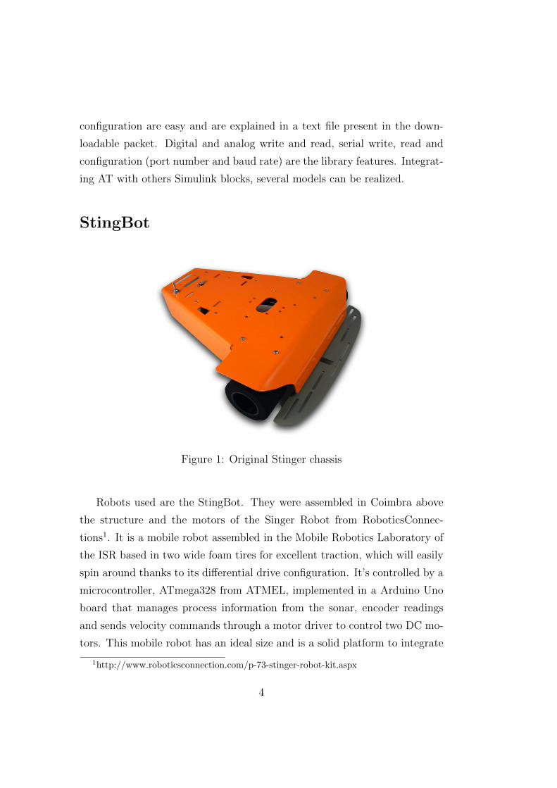
Figure 1: Original Stinger chassis
Robots used are the StingBot. They were assembled in Coimbra above
the structure and the motors of the Singer Robot from RoboticsConnec-
tions1. It is a mobile robot assembled in the Mobile Robotics Laboratory of
the ISR based in two wide foam tires for excellent traction, which will easily
spin around thanks to its differential drive configuration. It’s controlled by a
microcontroller, ATmega328 from ATMEL, implemented in a Arduino Uno
board that manages process information from the sonar, encoder readings
and sends velocity commands through a motor driver to control two DC mo-
tors. This mobile robot has an ideal size and is a solid platform to integrate
1http://www.roboticsconnection.com/p-73-stinger-robot-kit.aspx
4
adequate sensors to perform mobile robot ground routines.
Outline of the document
The document is divided in four main parts: the first evaluates the vari-
ous environments and programming languages existing in the world of robot
communications, explains also why the couple Matlab-Arduino was chosen;
a second shows and presents the AT library, with relative pros e cons; After
that there is a concise description of the robots of the laboratory and in the
final part all the results, the tests done, the difficulties met and the possible
future works that can be done are presented.
5

Chapter 1
Programming languages for
robotics
The appropriate languages, structures, and software architectures for de-
veloping robot software has been the topic of debate and discussion since
the earliest computer-controlled robot systems. These languages attempt to
reach a compromise, offering the ability to program low-level behavior in
some detail, while at the same time providing language abstractions that
facilitate the description of higher-level system behavior. Now the main lan-
guages available in the programming world will be presented, emphasizing
positive and negative characteristics and dividing them into different types.
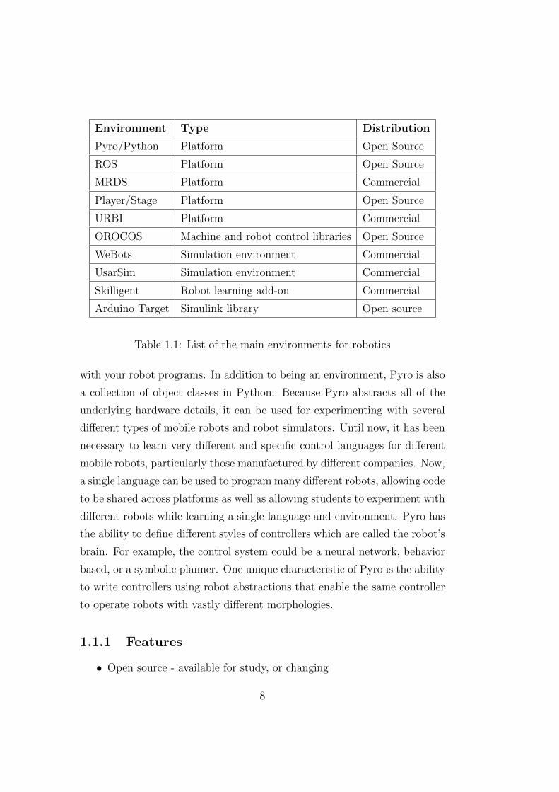
Table 1.1 shows the main environments, with their type and distribution.
After that every one of them will be briefly described.
1.1 Pyro
Pyro stands for Python Robotics. The goal of the project is to provide
a programming environment for easily exploring advanced topics in artifi-
cial intelligence and robotics without having to worry about the low-level
details of the underlying hardware. Pyro is written in Python. Python is
an interpreted language, which means that you can experiment interactively
7
Environment Type Distribution
Pyro/Python Platform Open Source
ROS Platform Open Source
MRDS Platform Commercial
Player/Stage Platform Open Source
URBI Platform Commercial
OROCOS Machine and robot control libraries Open Source
WeBots Simulation environment Commercial
UsarSim Simulation environment Commercial
Skilligent Robot learning add-on Commercial
Arduino Target Simulink library Open source
Table 1.1: List of the main environments for robotics
with your robot programs. In addition to being an environment, Pyro is also
a collection of object classes in Python. Because Pyro abstracts all of the
underlying hardware details, it can be used for experimenting with several
different types of mobile robots and robot simulators. Until now, it has been
necessary to learn very different and specific control languages for different
mobile robots, particularly those manufactured by different companies. Now,
a single language can be used to program many different robots, allowing code
to be shared across platforms as well as allowing students to experiment with
different robots while learning a single language and environment. Pyro has
the ability to define different styles of controllers which are called the robot’s
brain. For example, the control system could be a neural network, behavior
based, or a symbolic planner. One unique characteristic of Pyro is the ability
to write controllers using robot abstractions that enable the same controller
to operate robots with vastly different morphologies.
1.1.1 Features
• Open source - available for study, or changing
8
• Designed for students, faculty and researchers
• Works on many real robotics platforms and simulators
• Extensive course modules include control methods, vision (motion track-
ing, blobs, etc.), learning (neural networks, reinforcement learning, self-
organizing maps, etc.), evolutionary algorithms, and more.
1.1.2 Phyton
Python is a general-purpose, high-level programming language whose de-
sign philosophy emphasizes code readability. Its syntax is said to be clear
and expressive. Python has a large and comprehensive standard library.
Python supports multiple programming paradigms, primarily but not lim-
ited to object-oriented, imperative and, to a lesser extent, functional pro-
gramming styles. It features a fully dynamic type system and automatic
memory management, similar to that of Scheme, Ruby, Perl, and Tcl. Like
other dynamic languages, Python is often used as a scripting language, but
is also used in a wide range of non-scripting contexts.
1.1.3 Pros & Cons
Python is open source, so the free availability is the best positive feature
of this language. Has a stable version since more time than others. Has a
good support for objects, modules, and other reusability mechanisms. Lastly
permits an easy integration with and extensibility using C and Java. On the
other side the developers community using Python is pretty small compared
to other languages. Software performances ( benchmarks tests ) are nothing
special and there is also a great lack: no true multiprocessor support. More-
over, the absence of a commercial support point, even for an Open Source
project doesn’t permit a fast spread of the product.
9
1.2 ROS
Robot Operating System (ROS) is a software framework for robot soft-
ware development, providing operating system-like functionality on a het-
erogenous computer cluster. ROS was originally developed in 2007 under
the name switchyard by the Stanford Artificial Intelligence Laboratory in
support of the Stanford AI Robot project. As of 2008, development con-
tinues primarily at Willow Garage, a robotics research institute/incubator,
with more than twenty institutions collaborating in a federated development
model.
1.2.1 Features
The philosophical goals of ROS can be summarized as:
• Peer-to-peer
• Tools-based
• Multi-lingual
• Thin
• Free and open source
1.2.2 Nomenclature
The fundamental concepts of the ROS implementation are nodes, mes-
sages, topics, and services. Nodes communicate with each other by passing
messages. A message is a strictly typed data structure. Standard primitives
types (integer, floating point, boolean etc.) are supported. Message can be
composed of other messages, and arrays of other messages, nested arbitrarily
deep. A node sends a message by publishing it to a given topic or “map”.
A node that is interested in a certain kind of data will subscribe to the ap-
propriate topic. There may be multiple concurrent publisher and subscribers
10
for a single topic. In general, publishers and subscribers are not aware of
each others’ existence. Although the topic-based publish-subscribe model is
a flexible communications paradigm, its “broadcast” routing scheme is not
appropriate for synchronous transactions, which can simplify the design of
some nodes. In ROS, this is called service, defined by a string name and a
pair of strictly typed messages: one for the request and one for the response.
1.2.3 Pros & Cons
Code written for ROS is thin and can be used with other robot software
frameworks. More, the ROS framework is easy to implement in any modern
programming language (Python , C++). Easy testing: ROS has a built-in
unit/integration test framework called ROStest that makes it easy to bring
up and tear down test fixtures. ROS is appropriate for large runtime sys-
tems and for large development processes. Even if it has all those positive
aspects, a very great learning time is required to use well and dominate ROS.
Furthermore, there is the need of high processing time and memory to run
large algorithmos, such as the navigation stack.
1.3 Microsoft Robotics Developer Studio
MSRDS is powered by the strength of the C++ programming language
and the rich .NET framework.
MSRDS comprises of the following:
• DSS: Decentralised Software Services
• CCR: Concurrency and Co-ordination Runtime
• VPL: Visual Programming Language
• VSE: Visual Simulation Environment
11
1.3.1 DSS
It is a lightweigth runtime environment that sits on top of the CCR. It
provides robustness by providing advanced error-handling features. Partial
failures in sub-part of a system can lead to a complete halting of the whole
system.
1.3.2 CCR
It addresses the need to manage asynchronous operations, deal with con-
currency, exploit parallelism and deal with partial failure. Applications which
use CCR needs to coordinate through messages, deal with complex failure
scenarios, or in other words has to deal with asynchronous programming.
1.3.3 VPL
It is a GUI based programming logic system. It is actually a graphical
data-flow programming model. The exact logic of the program is represented
as sequences of blocks with inputs and outputs, which are connected.
1.3.4 VSE
The VSE provides the simulation to substitute hardware. Hardware has
multiple disadvantages like high cost, difficulty of debugging and tough to be
worked upon concurrently. Whereas simulation has a low barrier to entry and
its very easy prototype and test out new ideas. At the same time simulation
has a lack of noisy data i.e. assumes a perfect world and it is also tough to
model a hardware absolutely perfectly.
1.3.5 Pros & Cons
MSRDS has got extremely efficient backend with fantastic simulator and
with the added vantage of the VPL, robotics applications have become very
easy to compose. But at the same time, knowledge of coding is required
12
for some significant work. It also doesn’t provide any special support for
real-time applications.
1.4 Player/Stage
The Player/Stage project has got client side and modular architecture.
Player supports C, C++, Tcl, Python and Java. The system is a queue-based
message passing one. Each driver has a single incoming queue and they can
send messages on the queues if others.
1.4.1 Stage Simulation Environment
Player/Stage has got 3D rendering abilities, it is basically a 2D environ-
ment with a concept of elevation. It is like a plugin that connects to the
Player server just in the same manner as the hardware would have connected
to it. The Stage simulator tricks the Player Server by substituting the hard-
ware and cloning the drivers. It permits to reduce the high costs of the
hardware. The major features of Stage are:
• Optimal fidelity : it looks more into performance than accuracy
• Linear Scaling with Population: the algorythms are such designed that
they do not depend on the number of the robots
• Configurable device models : The sensor models are modeled with a lot
of flexibility and to conform as much closely as possible to the actual
nature of the hardware. They are fully configurable as much as the
original hardware provides
• Abstraction from Client mode: The sensors are available through the
Player interface, hence the client code cannot distinguish from the real
sensors or the simulated sensors.
13
1.4.2 Pros & Cons
The ease of use and the simplicity along with the usage of programming
language makes it a very popular platform amidst academicians and hob-
byists. On the contrary, the absence of robustness, missing constraints of
real-time demands, inability to be ported cleanly Windows platform and the
difficulty of installation causes an obstacle for its popularity.
1.5 Urbi
URBI stands for Universal Real Time Behaviour Interface, and is devel-
oped by a french company named Gostai. Their mission is to provide the
users with the best universal robotic platform. URBI’s observation is that
we are entering the robotic age and still there is incompatibility in terms of
software for the available hardware of robotics. The platform should work
with any robot, operating system or programming environment. URBI is
a quite innovation in the programming world as it not just a programming
language (urbiScript) but also has a component architecture (UObject) and
also several graphics programming tools (urbiStudio).
1.5.1 Pros & Cons
The main advantage of the product is the ease with which parallelism
and event handling can de done. The disadvantage would include the path
of having to learn a new language. It does have the facility to integrate with
other languages, but it doesn’t give the full control to those languages.
1.6 OROCOS
OROCOS stands for Open Robot Control Software. Their aim is to
build a generic modular framework for robot and machine control. They just
14
provide libraries for building but does not strictly provide a platform. The
design philosophy is centered around four main libraries:
• Real Time Toolkit (RTT)
• Orocos Components Library (OCL)
• Kinematics and Dynamics Library (KDL)
• Bayesian filtering library (BFL)
1.6.1 Pros & Cons
It is a platform that takes deep care of realtime applications. Unfortu-
nately, it is not a platform as a whole. Yet, for those who want accurate
results, and a perfect simulation, this is the best library to look out for.
1.7 WeBots
Webots is a development environment used to model, program and simu-
late mobile robots. With Webots the user can design complex robotic setups,
with one or several, similar or different robots, in a shared environment. The
properties of each object, such as shape, color, texture, mass, friction, etc.,
are chosen by the user. A large choice of simulated sensors and actuators
is available to equip each robot. The robot controllers can be programmed
with the built-in IDE or with third party development environments. The
robot behavior can be tested in physically realistic worlds. The controller
programs can optionally be transferred to commercially available real robots.
1.7.1 Features
Webots is a portable robot simulator: it runs natively on Windows, Mac
and Linux. Both world files and API functions are cross-platform: they can
easily be shared by people using different operating systems.
15
1.8 Usarsim
UsarSim is a 3D simulator oriented to the rescue robot, developed as a
research tool in a project of the US National Science Foundation. UsarSim
is faithfully reproduced in an environment of robotic assistance, including a
number of arenas, robot and all the necessary sensors. The simulator was
designed as an extension of the game engine, Unreal Engine, a commercial
software platform oriented to develop multiplayer first-person shooter de-
veloped by Epic Games. UsarSim defers completely to the Unreal Engine
scene graph rendering three-dimensional simulation of the physical interac-
tions between objects. In this way, leaving the most difficult aspects of the
simulation to a commercial platform can provide a visual rendering upper
and a good physical modeling, all efforts in developing UsarSim have focused
on the specific tasks of robotics, such as modeling of environments, sensors,
control systems and interface tools. Furthermore, the development is facil-
itated by the use of advanced editing software built into the game engine,
which the editor Unreal Editor and Unreal Script scripting language.
1.9 Skilligent
Skilligent’s software product is a control system which allows service
robots to interact with users (humans), learn new tasks and skills from hu-
mans, safely navigate in the environment, see objects and track them, use a
robotic arm, and perform other functions. The software packages are built to
run on control computers of autonomous multi-task service robots. The soft-
ware enables building multi-task autonomous robots which can learn proce-
dures and skills directly from human users while maintaining a social contact
with them. The software includes a robotic behavior control and coordina-
tion system with task and skill learning functions, a powerful robot vision
system, a visual localization system, a social human-to-machine interface,
a database for storing knowledge, an operator control unit software, and
16
other integrated components. The software has been specifically designed
for straightforward integration into PC-controlled robots and is based on re-
cent advances in understanding of embodied cognition, grounded perception,
robot learning, behavior coordination and human-to-machine interaction.
1.10 Our choice: Arduino Target... Why?
Every introduced environment has got many positive qualities and po-
tentialities. However, for this study the choice was on the couple Arduino
Target + Simulink. There are multiple reasons. First of all: AT is used
with an Arduino board; this means that AT was born to be an open source
project. Every part of code written in Arduino language is open source, and
so is AT. Moreover, the Arduino user community (both professional and am-
ateur) is very large. Another reason is that AT is a Simulink library, which
works in Matlab. Matlab has become an academic standard software and
most of engineering students all over the world know Matlab or use it. That
means that projects concerning AT could be easily diffused on a large scale.
Lastly, the simplicity: a block scheme. No programming language to know,
no lines and lines of commands to write; only linking blocks and setting their
parameters. AT can be very attractive for people that would have a first soft
contact with Arduino without having to study how to program the boards.
1.11 Summary
There is a great number of programming languages and environments in
the robot-programming world. Our choice is Arduino Target, a library of
blocks for Simulink. Its connection with Arduino and Matlab makes it a po-
tentially great project for future developments. In the next section the library
will be briefly presented, showing how to install it, which is the downloadable
stuff, and its limitations.
17

18

Chapter 2
Arduino Target
It consists of blocks which can be part of a model to build for Arduino
directly from Simulink. AT is downloadable for free from MathWorks1. In-
stallation and configuration are pretty simple and a .txt file that can be found
in the downloaded packet explains how to do them.
2.1 Installation
Before proceeding with the AT installation it is necessary to install the
Arduino IDE and Drivers, both downloadable from the Arduino website2.
The last version of the IDE can be found, but to work with AT it is necessary
to use a previous version (the arduino-0023 version worked well );
In the Appendix A it is possibile to find the steps to follow to configure
AT on Matlab.
2.2 The downlodable packet
Besides of the installation tutorial and a license text file, there are three
directories. The first one contains the system file of the library: “m” files,
1http://www.mathworks.com/matlabcentral/fileexchange/302772http://arduino.cc/en/Main/Software
19

“tlc” files and makefiles. The second one contains the files of the blocks
of AT (c,h, tlc,mex32 and mex64 files). Finally, the demos-directory: a few
demo-models to understand how to work with the library.Tcl, c and mex files
for new blocks can be generated with a MATLAB Tool: the Legacy Code,
that permits to create a MATLAB structure for registering the specification
for existing C or C++ code and the S-function being generated. In addition,
the function can generate, compile and link, and create a masked block for
the specified S-function. This will be described later.
2.3 Actual state of the library: blocks
AT consists of 7 blocks:
• Digital Input
• Digital Output
• Analog Input
• Analog Output
• Serial Read
• Serial Write
• Serial Configuration
2.4 Objectives
The objective of this work is to study deeply the library to understand
what it is possibile to do with the already present blocks. More: begin
to produce diagrams more complex than the demonstrative ones (already
available in the package) to perform new actions, try to avoid the limitations
of the library and start to think about expanding the library with new blocks.
20

Figure 2.1: Arduino Target Blocks
2.5 Limtations
AT is a library with great potentials. With it a user could theoretically
create any type of executable to send to an Arduino board without using the
Arduino programming language. So, programming Arduino without knowing
a single word of a programming language. But nowadays still has got a lot
of limitations and can be considered only a future great product that has to
be improved.
The on-line documentation is nearly absent; it consists only of the few
demos already present in the downloadable content. There isn’t any other
description of the product, of the blocks and of their limitations.
For being a relatively new product, only a few people is using it and
21

so help is difficult to find on forums or on-line communities. Furthermore,
the communication with MathWorks and its on-line help-center isn’t easy:
they never respond in a short time and most of the answers are authomatic
(generated by bots) or not helpful.
For our purpose there is also another great limitation: for the moment AT
doesn’t permit to have access to all the peripherals and features of Arduino.
So it isn’t possible to use them in a Simulink model.
In the following sections of the report further descriptions of the blocks
will be given. I will also talk about the possibility of create new blocks
using Arduino code and the Legacy Code Tool and the problems encountered
during my period of study of AT.
2.6 Summary
AT has only a few blocks for the moment, but is a really simple to be
used and installed in Matlab. A user with a good knowledge of the Simulink
blocks could realize interesting models, though the complexity is limited by
the small number of Arduino functions of the library. The aim is to insert
more Arduino functions in the AT blocks, even if a direct Arduino libraries
compilation will be necessary. The main goal is to manage to communicate
directly with the robots of the laboratory using Simulink models with AT
blocks. The robots we use in our university will be presented in the following
section.
22
Chapter 3
StingBot
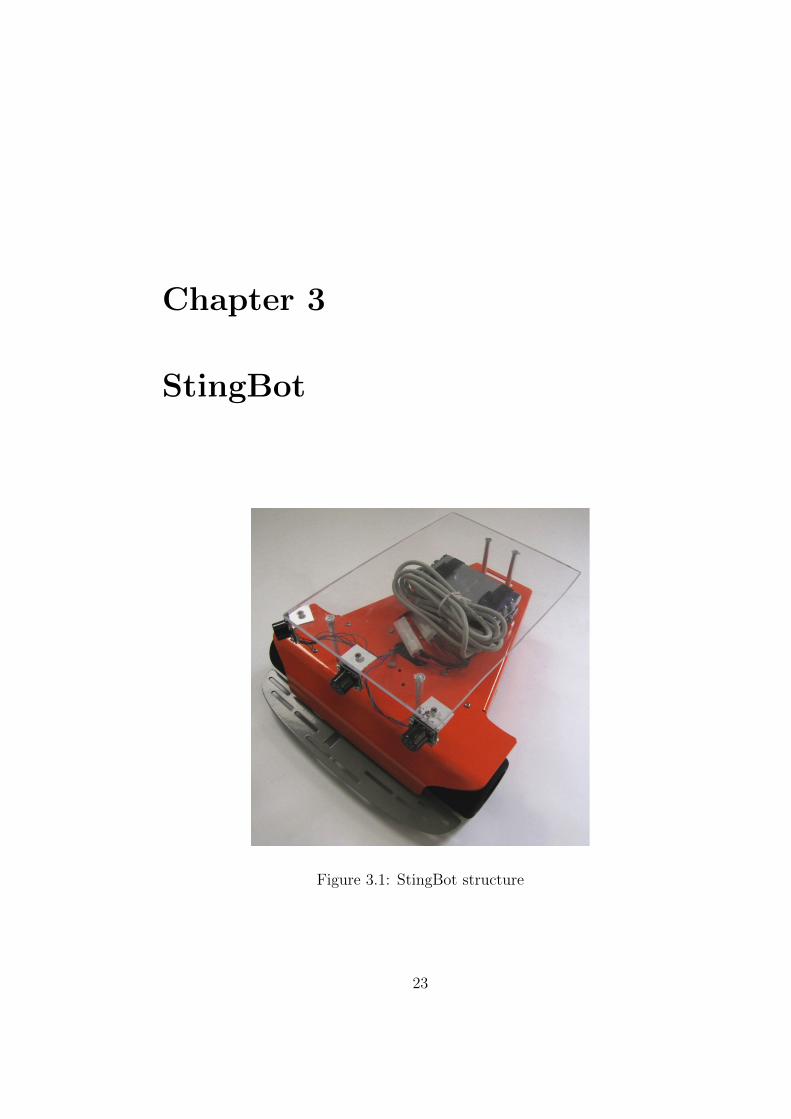
Figure 3.1: StingBot structure
23

3.1 General description
The robotic platform is a differential drive system (non-holonomic robot)
built upon the StingBot Robot Kit, equipped with 2 DC gearhead motors
with quadrature wheel encoders. The following figure gives a general view of
the StingBot Robot.
The StingBot Robot is equipped with:
• 3x Maxbotix Sonars MB1300
• Arduino Uno with ATmega328
• Motor drive Omni 3MD
• ZigBee module – Xbee Arduino Shield
• 2x DC Gearhead Motor with Quadrature Encoder
• 2x Battery Ni-MH pack 9.6V 2300mAh
• Foam tires
The processing and control units are the Arduino Uno with a XBee shield
module and the motor drive OMNI-3MD, which are located inside the Sting-
Bot chassis. The battery pack is placed above the chassis, between the shield
and the acrylic support and held together by two strips of velcro on the out-
side for easy access and replacement. The circuit switch power is located in
the back of the platform. Table 3.1 presents some hardware specifications.
24

Specification Value Unit
Voltage Range 9-14 V
Electric Current in Operation 1200 mA
Electric Current in Standby 110 mA
Maximum Speed 0,95 m/s
Weight 879 g
Weight with notebook 1990 g
Width 260 mm
Length 235 mm
Height 125 mm
Table 3.1: Hardware Specifications of the StingBot
3.2 Main schematic system
The processing unit consists of an Arduino Uno board equipped with
a microcontroller ATmega 328p from Atmel, which controls the platform’s
motion through the use of the Bot’n Roll OMNI-3MD board. For range
sensing, the robot uses Maxbotix Sonars MB1300 with a maximum range of
approximately 6 meters, which can have a configurable disposition with the
possibility of using up to 4 sonars in one platform using the analog ports of
the Arduino Uno board. For range sensing, the robot uses Maxbotix Sonars
MB1300 with a maximum range of approximately 6 meters, which can have
a configurable disposition with the possibility of using up to 4 sonars in one
platform using the analog ports of the Arduino Uno board. Additionally, to
enable point-to-point communication between robots, the Xbee Shield, con-
sisting on a ZigBee communication antenna attached on top of the Arduino
Uno board as an expansion module, was also incorporated. As for power
source, two packs of 9.6V 2300mAh Ni-MH batteries are deployed above the
chassis of each robot to ensure good autonomy. Finally, the platform also has
the possibility of including a 10” netbook on top of an acrylic support, which
extends the processing power and provides more flexibility. In our case, an
25

Figure 3.2: Main control circuit
ASUS eeePC 1001PXD BLACK N455 is used due to its reduced price and
size. Using the netbook has the advantage of enabling communication via
Wireless WiFi 802.11 b/g/n. Moreover, the netbook’s battery does not limit
the autonomy of the platform, since it can operate autonomously for around
6 hours.
3.3 What can be done with StingBot and ac-
tual AT library
The main operation that can be done using AT blocks is the serial com-
munication. It was tested using various communication velocities and gave
always great performances. In the next section I’ll show the Simulink block-
diagrams to use to perform various types of serial communications, with
examples and descriptions. It is possible to receive from Arduino (and send
26

to) digital and anagogic data that can be read on the screen directly from a
Simulink scope or that can be saved in a Matlab variable in order to create
a report of the experiences done.
3.3.1 StingBot sonars
Figure 3.3: StingBot 3d model
The Maxbotix MB1300 range sonar provides very short (15.24cm) to
long-distance (645.16cm) detection and ranging, with 2.54cm resolution. The
interface format used is the analog output. Among the advantages of this
device, it insures a reliable and stable range data, it is a very low cost sonar,
with virtually gone dead zone, one of the gold mark of this sensor. It also
has the very low power ranger, which is excellent for the battery system
implemented in this project, with a fast measurement cycle with readings
that can occur up to every 50ms (20-Hz rate), which are reported the range
reading directly, freeing up user processor.
27
Main features:
• Continuously variable gain for beam control and side lobe suppression
• Object detection includes zero range objects
• 2.5V to 5.5V supply with 2mA typical current draw
• Sensor operate at 42KHz
• Free run operation can continually measure and output range informa-
tion
• Triggered operation provides the range reading as desired
Output used:
• AN: Outputs analog voltage with a scaling factor of (Vcc/512). A
supply of 5V yields 3.9mV/cm. and 3.3V yields 2.5mV/cm. The
output is buffered and corresponds to the most recent range data
• +5: Vcc – Operates on 2.5V - 5.5V. Recommended current capability
of 3mA for 5V, and 2mA for 3V
• GND: Return for the DC power supply. GND (& Vcc) must be ripple
and noise free for best operation
While moving in a space with obstacles, the robot can recognize the pres-
ence of the obstacles using the sonars and then communicate their distance
via the anagogic pins of Arduino (a distance-depending value is sent). Our
StingBot mounts three sonars but we can’t perform a simultaneous reading
of the three values. Fortunately (especially directly with Arduino code), the
readings are really fast (more than 10 per second), and so we have an al-
most immediate reading of the data from all the three sonars. In the next
chapter I’ll show the Simulink diagram used to perform the readings, and
the respective part of Arduino code used to test the sonars.
28

3.4 What can’t be done with StingBot and
actual AT library
AT library will be even more powerful if other Arduino functions could be
added to the blocks in an easy way. This would be fundamental to open for
example an I2C communication, that is necessary to communicate with the
robots and so to make them move in the space without using other hardware
or other languages like ROS (we would like to do all the operation within an
Arduino environment). The main idea is to compile Arduino code directly
from MATLAB using features that would be explained in the next section.
More, create new blocks to be added at the AT library; these blocks could
have all the Arduino functions we like in their source code. For the moment
it isn’t possible to do this last step, but the instruments and the features of
MATLAB that are under study are for sure the correct ones.
3.5 Summary
AT libraries and StingBot were briefly presented. In the following section
I’ll explain how to work with the Simulink blocks of the library, showing how
the blocks work and the various diagrams that can be created. Moreover,
useful features of MATLAB will be added to the projects in order to extend
the potentiality of the diagrams of blocks created.
29

30
Chapter 4
Experiments and results
In this section will be explicated all the functions of the AT blocks, and
the models obtained using them. Then will be presented the use of callback
functions within Simulink, and a brief “how to” about creating new blocks
compiling parts of Arduino code.
AT at the moment consists of “only” 7 blocks. It could seem a very low
number. However, because of being integrated in models using potentially
almost all other Simulink blocks, the library offers the possibility to obtain
great results, as far as developing complex schemes of blocks.
31
4.1 Build a model: what does it mean?
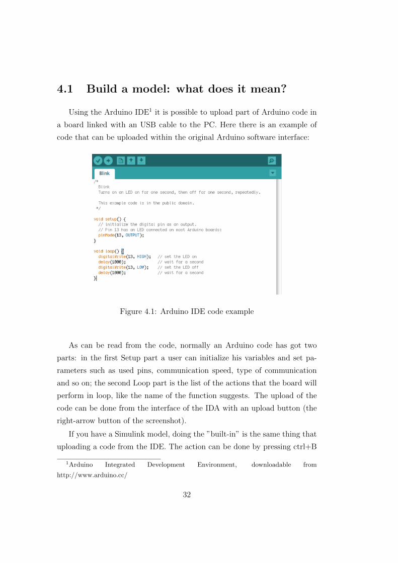
Using the Arduino IDE1 it is possible to upload part of Arduino code in
a board linked with an USB cable to the PC. Here there is an example of
code that can be uploaded within the original Arduino software interface:
Figure 4.1: Arduino IDE code example
As can be read from the code, normally an Arduino code has got two
parts: in the first Setup part a user can initialize his variables and set pa-
rameters such as used pins, communication speed, type of communication
and so on; the second Loop part is the list of the actions that the board will
perform in loop, like the name of the function suggests. The upload of the
code can be done from the interface of the IDA with an upload button (the
right-arrow button of the screenshot).
If you have a Simulink model, doing the ”built-in” is the same thing that
uploading a code from the IDE. The action can be done by pressing ctrl+B
1Arduino Integrated Development Environment, downloadable from
http://www.arduino.cc/
32
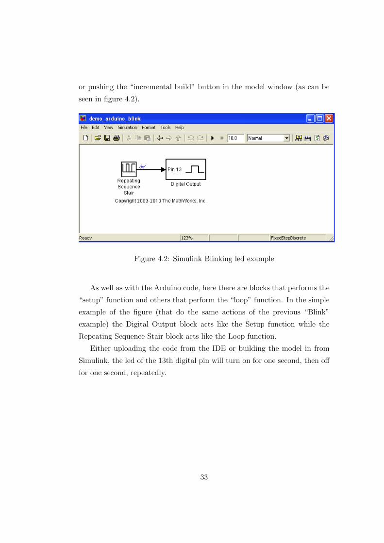
or pushing the “incremental build” button in the model window (as can be
seen in figure 4.2).
Figure 4.2: Simulink Blinking led example
As well as with the Arduino code, here there are blocks that performs the
“setup” function and others that perform the “loop” function. In the simple
example of the figure (that do the same actions of the previous “Blink”
example) the Digital Output block acts like the Setup function while the
Repeating Sequence Stair block acts like the Loop function.
Either uploading the code from the IDE or building the model in from
Simulink, the led of the 13th digital pin will turn on for one second, then off
for one second, repeatedly.
33
4.2 Serial communication
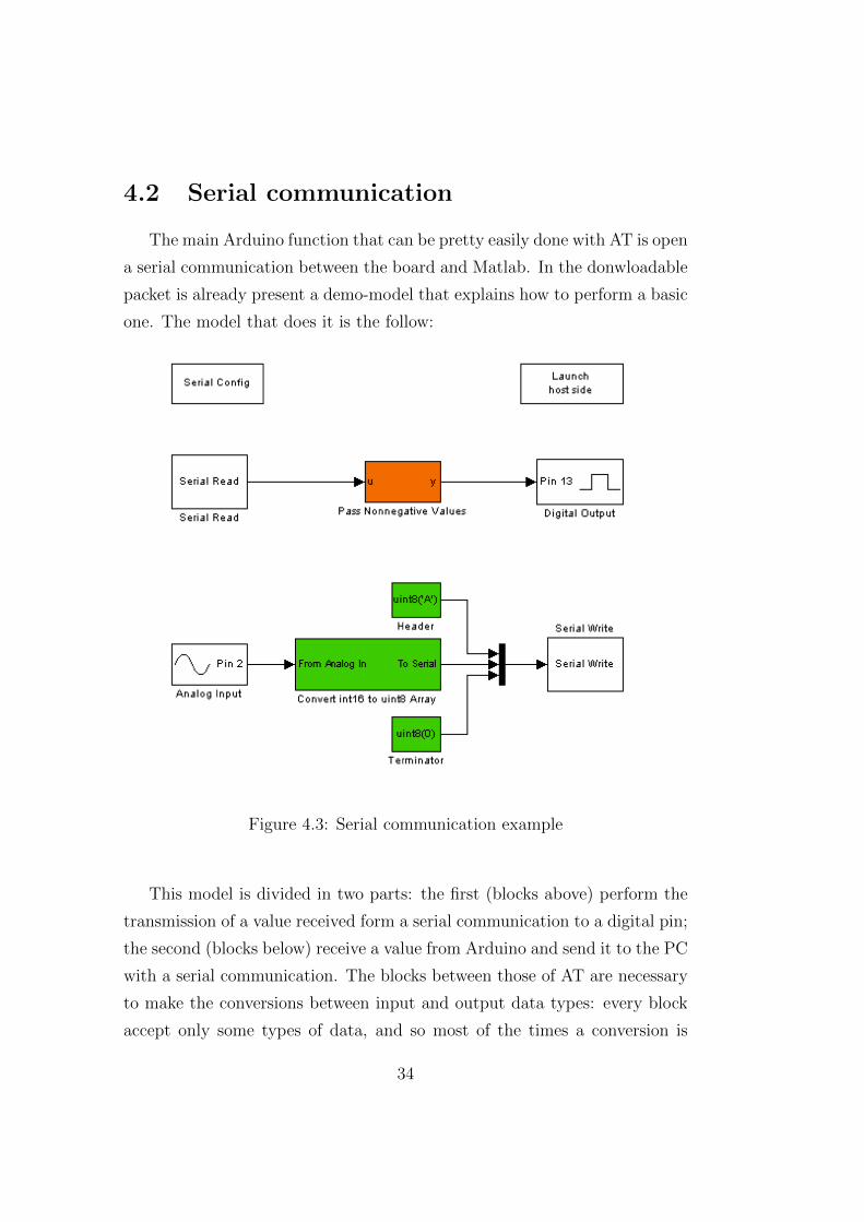
The main Arduino function that can be pretty easily done with AT is open
a serial communication between the board and Matlab. In the donwloadable
packet is already present a demo-model that explains how to perform a basic
one. The model that does it is the follow:
Figure 4.3: Serial communication example
This model is divided in two parts: the first (blocks above) perform the
transmission of a value received form a serial communication to a digital pin;
the second (blocks below) receive a value from Arduino and send it to the PC
with a serial communication. The blocks between those of AT are necessary
to make the conversions between input and output data types: every block
accept only some types of data, and so most of the times a conversion is
34

required. Analog Input block can be substituted with a Digital Input block
if a user wanted to read the state of a digital pin (high or low). When using
those Serial blocks of AT, also the Serial Config block is necessary. With it,
the speed of the communication can be chosen.
35

4.3 Server/Host system
To perform simulations, the users have to set up a couple of server/host
models. What I mean is a first block that is built in the board and provide
the board of the loop function(s); a second block that receive and send signals
from/to the board. It can be done through a serial communication between
Arduino and Matlab. Doing this the host block can perform several things:
measure the level of an analog pin, evaluate the state of a digital pin, count
the state variations of the pins and so on.
A simple host demo-model equipped in the AT library is the follow:
Figure 4.4: Serial communication: host blocks diagram
The model is clearly strictly connected with the first presented one. Serial
Send block send the value that will be written in the digital pin 13 and the
Serial Receive block read the value from the Analog pin 2. It is important
to think about a “off-state” of the communication, here realized with a 0
constant value and a switch. Normally, without the possibility to put the
simulation into a off state, Matlab will send some kind of errors and will
36
not permit to perform the simulation. Display or Scope blocks are really
useful to analyze graphically the input signals that we receive with a serial
communication from Arudino.
4.4 Circuit examples
Using a few electric parts and a breadboard we can realize small circuits
and create Simulink models that substitute a lot of Arduino Code:
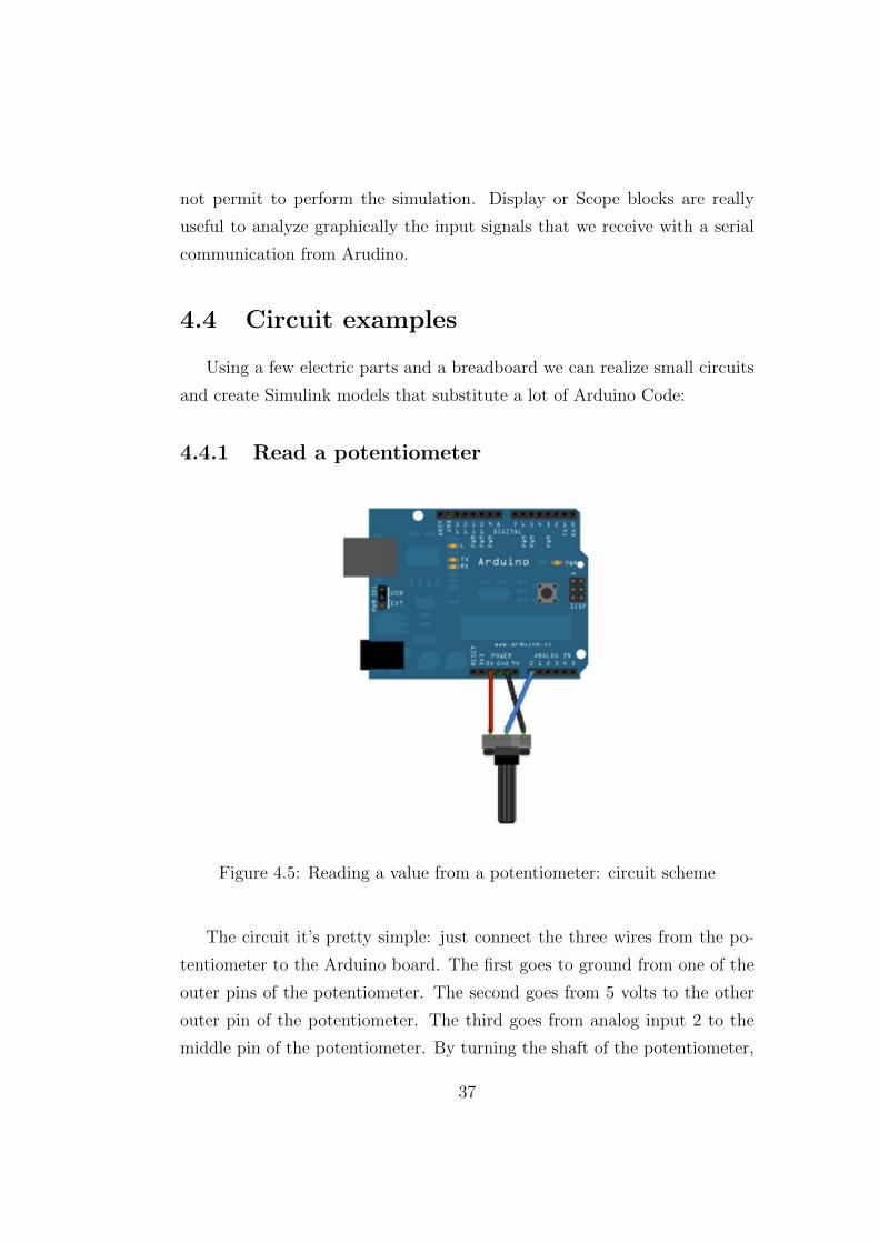
4.4.1 Read a potentiometer
Figure 4.5: Reading a value from a potentiometer: circuit scheme
The circuit it’s pretty simple: just connect the three wires from the po-
tentiometer to the Arduino board. The first goes to ground from one of the
outer pins of the potentiometer. The second goes from 5 volts to the other
outer pin of the potentiometer. The third goes from analog input 2 to the
middle pin of the potentiometer. By turning the shaft of the potentiometer,
37

it is possible to change the amount of resistance on either side of the wiper
which is connected to the center pin of the potentiometer. This changes the
voltage at the center pin. When the resistance between the center and the
side connected to 5 volts is close to zero (and the resistance on the other side
is close to 10 kiloohms), the voltage at the center pin nears 5 volts. When
the resistances are reversed, the voltage at the center pin nears 0 volts, or
ground. This voltage is the analog voltage that we are reading as an input.
Simulink model
In this case the server part of the project can be the same as before. We
just have to send the read value from an Analog Pin to the Serial Write block.
In the Host part (figure 4.6), we can add an Embedded Matlab Function block
to send to the serial port values depending of the received one (for example
we can send a ”1” to the digital pin 13 if the value from the potentiometer
is higher than a preset value). In the example we can also read the value
directly on the Simulink windows from the Display block. The function that
use can be like the following:
Figure 4.6: Reading a value from a potentiometer: Simulink diagram
38

Corresponding Arduino code
With this Simulink model a lot of Arduino code is substituted. Here are
the corresponding lines (with comment that explain the code):
/*
AnalogReadSerial
Reads an analog input on pin 0, prints the result
to the serial monitor.
Attach the center pin of a potentiometer to pin A0,
and the outside pins to +5V and ground.
This example code is in the public domain.
*/
// the setup routine runs once when you press reset:
void setup() {
// initialize serial communication at 9600 bits per second:
Serial.begin(9600);
}
// the loop routine runs over and over again forever:
void loop() {
// read the input on analog pin 0:
int sensorValue = analogRead(A0);
// print out the value you read:
Serial.println(sensorValue);
delay(1); // delay in between reads for stability
}
39

Embedded coder
Embedded Matlab is a subset of the Matlab language that supports effi-
cient code generation for deployment in embedded systems and acceleration
of fixed-point algorithms. In the Simulink environment it appears like a
block in which you can write your own Matlab function that uses the inputs
to generate depending outputs.
Embedded MATLAB does not support the following MATLAB features:
• Cell arrays
• Command/function duality
• Dynamic variables
• Global variables
• Java
• Matrix deletion
• Nested functions
• Objects
• Sparse matrices
• Try/catch statements
Even with those limitations, is a very useful mode to work with the signals
received without having to think about additional blocks to look for in the
Simulink Library. The blocks of the Embedded coder can be found in the
“user-defined functions” Simulink section.
40

4.4.2 Digital counter
Figure 4.7: Button State Change Detection (Edge Detection): Circuit scheme
Connect three wires to the Arduino board. The first goes from one leg
of the pushbutton through a pull-down resistor (here 10 KOhms) to ground.
The second goes from the corresponding leg of the pushbutton to the 5 volt
supply. The third connects to a digital i/o pin (here pin 2) which reads
the button’s state. When the pushbutton is open (unpressed) there is no
connection between the two legs of the pushbutton, so the pin is connected
to ground (through the pull-down resistor) and we read a LOW. When the
button is closed (pressed), it makes a connection between its two legs, con-
necting the pin to voltage, so that we read a HIGH. (The pin is still connected
to ground, but the resistor resists the flow of current, so the path of least
resistance is to +5V).
Simulink model
To perform the count of the changes of state of the digital pin we can
use the Counter Block. It has various parameters to be set: count direction,
41
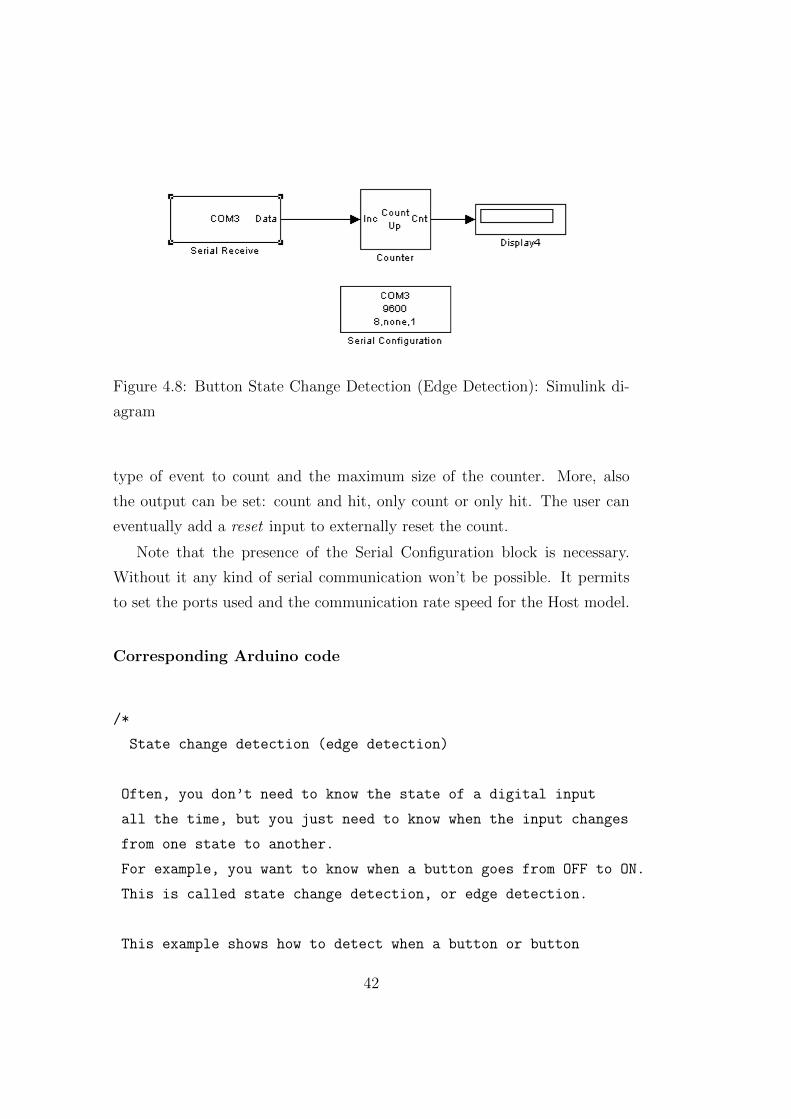
Figure 4.8: Button State Change Detection (Edge Detection): Simulink di-
agram
type of event to count and the maximum size of the counter. More, also
the output can be set: count and hit, only count or only hit. The user can
eventually add a reset input to externally reset the count.
Note that the presence of the Serial Configuration block is necessary.
Without it any kind of serial communication won’t be possible. It permits
to set the ports used and the communication rate speed for the Host model.
Corresponding Arduino code
/*
State change detection (edge detection)
Often, you don’t need to know the state of a digital input
all the time, but you just need to know when the input changes
from one state to another.
For example, you want to know when a button goes from OFF to ON.
This is called state change detection, or edge detection.
This example shows how to detect when a button or button
42
changes from off to on and on to off.
The circuit:
* pushbutton attached to pin 2 from +5V
* 10K resistor attached to pin 2 from ground
* LED attached from pin 13 to ground (or use the built-in LED on
most Arduino boards)
created 27 Sep 2005
modified 30 Aug 2011
by Tom Igoe
This example code is in the public domain.
http://arduino.cc/en/Tutorial/ButtonStateChange
*/
// this constant won’t change:
const int buttonPin = 2;
const int ledPin = 13;
// Variables will change:
int buttonPushCounter = 0;
int buttonState = 0;
int lastButtonState = 0;
void setup() {
// initialize the button pin as a input:
pinMode(buttonPin, INPUT);
// initialize the LED as an output:
43

pinMode(ledPin, OUTPUT);
// initialize serial communication:
Serial.begin(9600);
}
void loop() {
// read the pushbutton input pin:
buttonState = digitalRead(buttonPin);
// compare the buttonState to its previous state
if (buttonState != lastButtonState) {
// if the state has changed, increment the counter
if (buttonState == HIGH) {
// if the current state is HIGH then the button
// wend from off to on:
buttonPushCounter++;
Serial.println("on");
Serial.print("number of button pushes: ");
Serial.println(buttonPushCounter);
}
else {
// if the current state is LOW then the button
// wend from on to off:
Serial.println("off");
}
}
// save the current state as the last state,
//for next time through the loop
lastButtonState = buttonState;
44

// turns on the LED every four button pushes by
// checking the modulo of the button push counter.
// the modulo function gives you the remainder of
// the division of two numbers:
if (buttonPushCounter % 4 == 0) {
digitalWrite(ledPin, HIGH);
} else {
digitalWrite(ledPin, LOW);
}
}
45
4.4.3 PWM
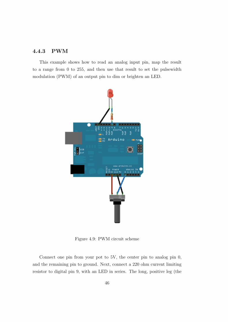
This example shows how to read an analog input pin, map the result
to a range from 0 to 255, and then use that result to set the pulsewidth
modulation (PWM) of an output pin to dim or brighten an LED.
Figure 4.9: PWM circuit scheme
Connect one pin from your pot to 5V, the center pin to analog pin 0,
and the remaining pin to ground. Next, connect a 220 ohm current limiting
resistor to digital pin 9, with an LED in series. The long, positive leg (the
46

anode) of the LED should be connected to the output from the resistor, with
the shorter, negative leg (the cathode) connected to ground.
Simulink model
Figure 4.10: PWM simulink diagram
We can perform this action in Simulink using the “variable delay event
genetator” block. It commands the “event counter” block that here is set on
0-1. The analog input determines the different delay wherewith the “event”
is created. This event is substantially a “1” to send to the output (that is
the digital pin where the led is connected). With this diagram I can make
a led bright at different speeds, only using a potentiometer that modifies an
analog input.
Corresponding Arduino code
/*
Analog input, analog output, serial output
Reads an analog input pin, maps the result to a range
from 0 to 255 and uses the result to set the pulsewidth
modulation (PWM) of an output pin.
Also prints the results to the serial monitor.
47
The circuit:
* potentiometer connected to analog pin 0.
Center pin of the potentiometer goes to the analog pin.
side pins of the potentiometer go to +5V and ground
* LED connected from digital pin 9 to ground
created 29 Dec. 2008
modified 9 Apr 2012
by Tom Igoe
This example code is in the public domain.
*/
// These constants won’t change. They’re used to give names
// to the pins used:
const int analogInPin = A0;
const int digitalOutPin = 9;
int sensorValue = 0;
int outputValue = 0;
void setup() {
// initialize serial communications at 9600 bps:
Serial.begin(9600);
}
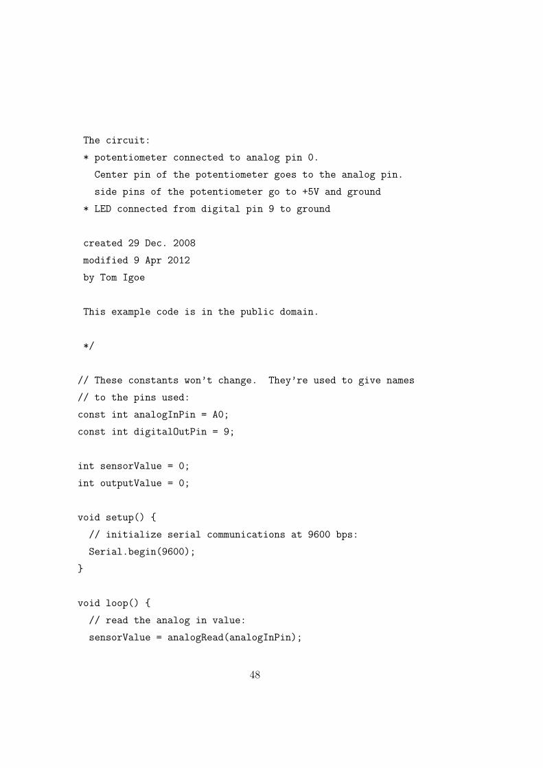
void loop() {
// read the analog in value:
sensorValue = analogRead(analogInPin);
48
// map it to the range of the analog out:
outputValue = map(sensorValue, 0, 1023, 0, 255);
// change the analog out value:
digitalWrite(analogOutPin, outputValue);
// wait 2 milliseconds before the next loop
// for the analog-to-digital converter to settle
// after the last reading:
delay(2);
}
49
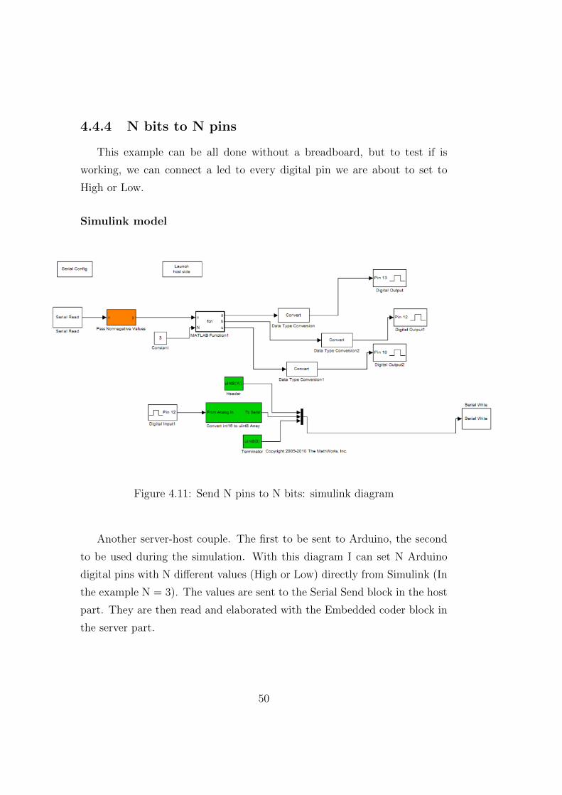
4.4.4 N bits to N pins
This example can be all done without a breadboard, but to test if is
working, we can connect a led to every digital pin we are about to set to
High or Low.
Simulink model
Figure 4.11: Send N pins to N bits: simulink diagram
Another server-host couple. The first to be sent to Arduino, the second
to be used during the simulation. With this diagram I can set N Arduino
digital pins with N different values (High or Low) directly from Simulink (In
the example N = 3). The values are sent to the Serial Send block in the host
part. They are then read and elaborated with the Embedded coder block in
the server part.
50

The function I wrote is the following2:
function[a,b,c] = fcn(u,N)
%#codegen
a = 0;
b = 0;
c = 0;
out = zeros(N);
for i = 1:N
att_val = 10^(N-i);
att_div = u./att_val;
if att_div == 1
out(N-i+1) = 1;
u = u-att_val;
end;
end;
a = out(3);
b = out(2);
c = out(1);
Also Data conversion blocks are necessary, because the various blocks of
the diagrams sometimes require different types of variables. We can test if
the simulation is working connecting leds to the digital bits used in the server
part. Also the Serial Write part in the Server diagram is used to test in the
2First I create a ”out” vector of zeros. It will have the same dimension of N, the number
of pins that I want to set. Than in the for cycle I take advantage of the input being a
decimal number with only 1 or 0 as digits. I subsequently divide it by powers of ten. If
the result is 1, I substitute the value of the actual element of ”out” with 1. At the end I
copy the values of the ”out” vector to the N output variables.
51

host model if the simulation is working well. In the host part we have only
to send the desired values. For example to set all three pins to High we have
to send a 111 (decimal); to set two pins to Low and one to High we have to
send a 1, a 10 or a 100, depending on which block we want to set on High
(sending 1 is the same that sending a 001 and sending 10 is the same that
sending a 010 ).
52
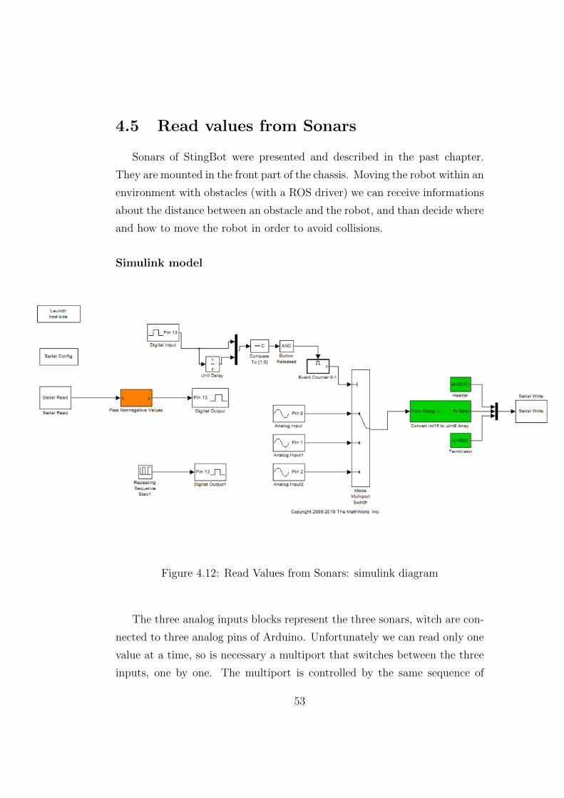
4.5 Read values from Sonars
Sonars of StingBot were presented and described in the past chapter.
They are mounted in the front part of the chassis. Moving the robot within an
environment with obstacles (with a ROS driver) we can receive informations
about the distance between an obstacle and the robot, and than decide where
and how to move the robot in order to avoid collisions.
Simulink model
Figure 4.12: Read Values from Sonars: simulink diagram
The three analog inputs blocks represent the three sonars, witch are con-
nected to three analog pins of Arduino. Unfortunately we can read only one
value at a time, so is necessary a multiport that switches between the three
inputs, one by one. The multiport is controlled by the same sequence of
53

blocks that we already used in the PWM example. The event that makes
the switch work is a “1” again. It is generated by a sequence of zeros and
ones (repeated stair sequence block). This sequence goes into a digital pin
of Arduino. This pin is input and output at the same time. First it receives
the zeros-ones sequence and then it controls the Event Counter block. The
switching speed between the three sonars depends on the sampling time that
I can set for the Repeated Stair Sequence block. Unfortunately it can’t be
lower than 0.1 seconds. For this reason I could read only 3 values per second
for every sonar, and this is a negative aspect in this case: performing the
same action directly with the Arduino IDE I could read a lot of more values
per second. In the host part where I actually read the values I can save the
data in MATLAB vectors of variables, in order to create a sort of report of
the simulation. It can be done using the “callback functions” of MATLAB.
They will be presented in the following section.
Corresponding Arduino code
This is the code that is used to test if the Sonars are working. With it
we can take the values from the sonars and read them on the serial monitor.
// Standard lib
#include <stdio.h>
#include <string.h>
#include <math.h>
/***************** Functions *****************/
// SONARS
int getRange(int pin_num) {
54
int aux_sensorValue=0, sensorValue=0, cnt=0;
int samples = 20;
delay(10);
while (cnt != samples) {
digitalWrite(12, HIGH); // Activate chain reading on sonars
sensorValue = analogRead(pin_num);
sensorValue = 1.767 * pow(sensorValue,0.9465) - 0.3759;
aux_sensorValue = aux_sensorValue + sensorValue;
cnt = cnt + 1;
digitalWrite(12, LOW);
}
cnt=0;
sensorValue = round( aux_sensorValue / samples);
return (sensorValue);
}
/***************** Setup *****************/
void setup()
{
Serial.begin(19200); //DEBUG on default serial port
55

/* Give 5v to power sonars, digital pin 13 */
pinMode(13, OUTPUT);
digitalWrite(13, HIGH);
/* Give 5v to digital pin 12 */
pinMode(12, OUTPUT);
digitalWrite(12, LOW);
delay(250); // Wait 250ms before reading sonars
}
void loop()
{
delay(500);
Serial.println(getRange(A0), DEC);
delay(10);
Serial.println(getRange(A1), DEC);
delay(10);
Serial.println(getRange(A2), DEC);
delay(10);
Serial.print("------\n");
}
56

4.6 Callback functions
Callback functions are a powerful way of customizing your Simulink model.
A callback is a function that executes when you perform various actions on
your model, such as clicking on a block or starting a simulation. You can use
callbacks to execute a MATLAB script or other MATLAB commands. You
can use block, port, or model parameters to specify callback functions.
Common tasks you can achieve by using callback functions include:
• Loading variables into the MATLAB workspace automatically when
you open your Simulink model
• Executing a MATLAB script by double-clicking on a block
• Executing a series of commands before starting a simulation
• Executing commands when a block diagram is closed
You can create model callback functions interactively or programmati-
cally. Use the Callbacks pane of the model’s Model Properties dialog box to
create model callbacks interactively. To create a callback programmatically,
use the set param command to assign a MATLAB expression that imple-
ments the function to the model parameter corresponding to the callback.
For example, the following command evaluates the variable testvar when the
user double-clicks the Test block in mymodel model:
set param(’mymodel/Test’, ’OpenFcn’, testvar)
You can examine the clutch system (sldemo clutch.mdl) for routines asso-
ciated with many model callbacks. This model defines the following callbacks:
• PreLoadFcn
• PostLoadFcn
57
• StartFcn
• StopFcn
• CloseFcn
There also also three useful function that can be used to start, pause or
continue the simulation when you perform one of the actions listed here:
• Set param (’mymodel/Test’, ‘SimulationCommand’, ‘start’)
• Set param (’mymodel/Test’, ‘SimulationCommand’, ‘pause)
• Set param (’mymodel/Test’, ‘SimulationCommand’, ‘continue)
The complete documentation can be found here :
http://www.mathworks.it/help/toolbox/simulink/ug/f4-122589.html
4.7 Legacy Code Tool
You can use the Simulink Legacy Code Tool to automatically generate
fully inlined C MEX S-functions for legacy or custom code that is optimized
for embedded components, such as device drivers and lookup tables, that call
existing C or C++ functions. You can use the tool to:
• Compile and build the generated S-function for simulation.
• Generate a masked S-Function block that is configured to call the ex-
isting external code.
If you want to include these types of S-functions in models for which you
intend to generate code, you must use the tool to generate a TLC block file.
The TLC block file specifies how the generated code for a model calls the ex-
isting C or C++ function. If the S-function depends on files in folders other
than the folder containing the S-function dynamically loadable executable
file, and you want to maintain those dependencies for building a model that
58

includes the S-function, use the tool to also generate an rtwmakecfg.m file
for the S-function. For example, for some applications, such as custom
targets, you might want to locate files in a target-specific location. The
Simulink Coder build process looks for the generated rtwmakecfg.m file in
the same folder as the S-function’s dynamically loadable executable and calls
the rtwmakecfg function if the software finds the file.
An example of how to compile an own C++ code using also Arduino
functions can be found in the Appendix B.
4.8 Summary
A valid simulator of Arduino Uno (usable in Simulink) doesn’t exist yet.
Testing models requires the presence of external components like a bread-
board, resistances, switches, leds etc. Anyway, with only a few of them it
is possible to realize and simulate pretty complex and interesting projects.
Those simulations are necessary to understand that the models we create are
good and can be exported to bigger projects. Beyond the blocks libraries,
Simulink and Matlab offer others tools that permit to improve our Arduino
experience, like callback functions and Legacy Code Tool. Even the study
of AT library isn’t completed yet and in the future it could become a more
complex and complete library, I will try to give a general opinion about
this product. In the following section also some ideas for future works and
improvements will be presented.
59

60

Chapter 5
Conclusion & Future works
I would say that AT is a great product. Once improved and diffused more
widely will be a library of great use also in academic field. Being integrated
in a blocks-scheme environment, it permits to perform many simulations of
many types in a short time. This fact also helps a lot when debugging. Block
and parameters of the models to debug can be substituted or variated easily,
in contrast to working with a programming language.
5.1 Conclusions
5.1.1 Cons...
The AT users community is still small but growing. For this reason is
still difficult to share information, projects and ideas with a wide group of
people. Furthermore, as I already said, the technical help of Mathworks
for AT is nearly absent, as well as a relative documentation. Documents
like this one, sorts of “how to” don’t exist or are very hard to find. There
are good news: Matworks released a few months ago a new version of the
library. There aren’t substantial differences with the older one at a first
sight, but for sure the code was a bit re-writted and some small bugs were
corrected. This fact could mean that AT is still an alive project and that
61
some Simulink/Arduino users started using it. Lastly, it is still hard to add
Arduino functions to new blocks, because of many compiling errors, but this
is for sure a work in progress.
5.1.2 ...& Pros
For sure AT has got much positive aspects than negative ones. It is inside
a completely open-source environment: AT code is open source in its own
and it works with Arduino, that was born to be a open-source project. An
open-source context permits to share data without limitations and helps a
fast development. Another positive aspect of the library is that it works
with Simulink, which is a Matworks product, integrated in Matlab. Matlab
nowadays is a worldwide known software and I think that realizing Arduino
projects could be part of informatics or electronics thesis. Even if aren’t
many, the already present blocks are very simple to use. They don’t require
practically any configuration (except very few parameters like the number of
a pin or the serial port used), and so a new user can start to work with the
AT library easily from the beginning, also without having a great knowledge
of Simulink or Matlab. Moreover, the possibility to use also useful Matlab
tools like the Embedded Coder and the Callback Functions give to the models
enormous potentiality.
5.2 Other platforms
Other two AT-like platforms were found on Matlab downloadable stuff.
They are very similar to the one I used in my study and it would be intrest-
ing to do a detailed comparison between them. For the moment the other
libraries were only mentioned, and weren’t used for lack of time. By the way,
they can be found here: http://www.mathworks.it/matlabcentral/fileexchange/35639
and here:
http://www.mathworks.it/matlabcentral/fileexchange/32374-matlab-support-
package-for-arduino-aka-arduinoio-package.
62

5.3 Future works and applications
As already anticipated, the main idea to improve AT library is to extend
the library with new blocks. We could create our own Arduino code, directly
compile it from MATLAB and then, using MATLAB tools like LCT, create
a new Simulink block that uses the Arduino functions from our code. The
possibility of adding other Arduino functions to the library would permit
to have access also to other features that can normally be done with Ar-
duino pins. In Appendix C there is a detailed description of the Uno Board.
One example is the external interrupt (with the function attachInterrupt() ):
imaging of moving the robot around, we can block the simulation using the
Callback Function, but having the possibility to use an external interrupt
directly in a block of a Simulink model the performances would be greater.
Figure 5.1: Communications in the motor driver/Stingbot/Arduino system
63

As can be seen in the figure the communication between motor driver,
robot ad Arduino is an I2C communication: Arduino can manage this type of
communication in its pins. More: with I2C we could move the robot without
using other programming languages, like ROS. Finally, StingBot has got also
a ZigBee module mounted over Arduino. Using functions of Arduino that
work with the ZigBee ca be useful to coordinate various robots together, if
they aren’t controlled with laptops mounted on the structure.
64

Appendix A
Arduino Target installation and
configuration
1. Unzip arduino.zip to a folder without spaces in its name, e.g. c:\ArduinoTarget
2. Add the subfolders arduiono, demos and block to the MATHLAB-
PATH, e.g. by typing the following command in the Matlab command
window:
>> cd c:\ArduinoTarget
>> addpath(fullfile(pwd,’arduino’),fullfile(‘block’),fullfile(‘demos’))
>> savepath
3. Type the following command to refresh Simulink customization:
>> sl refresh customizations
4. Connect your Arduino Board to the USB port
5. Set up the preferences. These are persistent across Matlab sessions, so
you don’t have to specify them each time you start Matlab.
• Specify location of the Arduino IDE
>> arduino.Prefs.setArduinoPath(‘c:\Program Files\arduino\arduino-
0023’)
65
• Specify Arduino Board (Duemilanove, Uno, Mega, etc.)
>> arduino.Prefs.setBoard % see list of board options
>> adruino.Prefs.setBoard(‘uno’)
• Find the COM port associated with Arduino
>> comPorts = arduino.Prefs.searchForComPort
If the above command doesn’t show any options, open Windows
Device Manager, navigate to “Ports (COM & LPT)”, and look
for ports labeled “USB Serial Port” or “Arduino”.
• Specify the COM port
>> arduino.Prefs.setComPort(‘COM9’)
• Open a demo model:
>> demo arduino blink
• 7. Build and deploy the executable by pressing Ctrl+B, or choos-
ing Tools>Code Generation>Build Model. If the deployment is
successful, you should see the LED connected to PIN 12 blinking
once per second.
Products Requiremens
Required MathWorks products:
R2011a or later:
• Matlab
• Simulink
• Matlab coder
• Simulink Coder
• Embedded Coder
Pre-R2011a:
66
• Matlab
• Simulink
• Real-Time Workshop
• Embedded Coder
Recommended MathWorks products:
• Instrument Control Toolbox(required for host-side Serial Send and Se-
rial Receive blocks)
• Stateflow
• Stateflow Coder (pre-R2011a)
Supported Platforms: Microsoft Windows 32-bit or 64-bit.
Supported Arduino Hardware:
• Uno
• Duemilanove (ATmega168 or ATmega328p)
• Mega (ATmega1280 or ATmega2560)
67

68
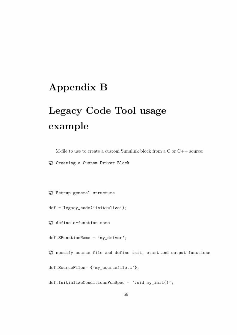
Appendix B
Legacy Code Tool usage
example
M-file to use to create a custom Simulink block from a C or C++ source:
%% Creating a Custom Driver Block
%% Set-up general structure
def = legacy_code(’initizlize’);
%% define s-function name
def.SFunctionName = ’my_driver’;
%% specify source file and define init, start and output functions
def.SourceFiles= {’my_sourcefile.c’};
def.InitializeConditionsFcnSpec = ’void my_init()’;
69
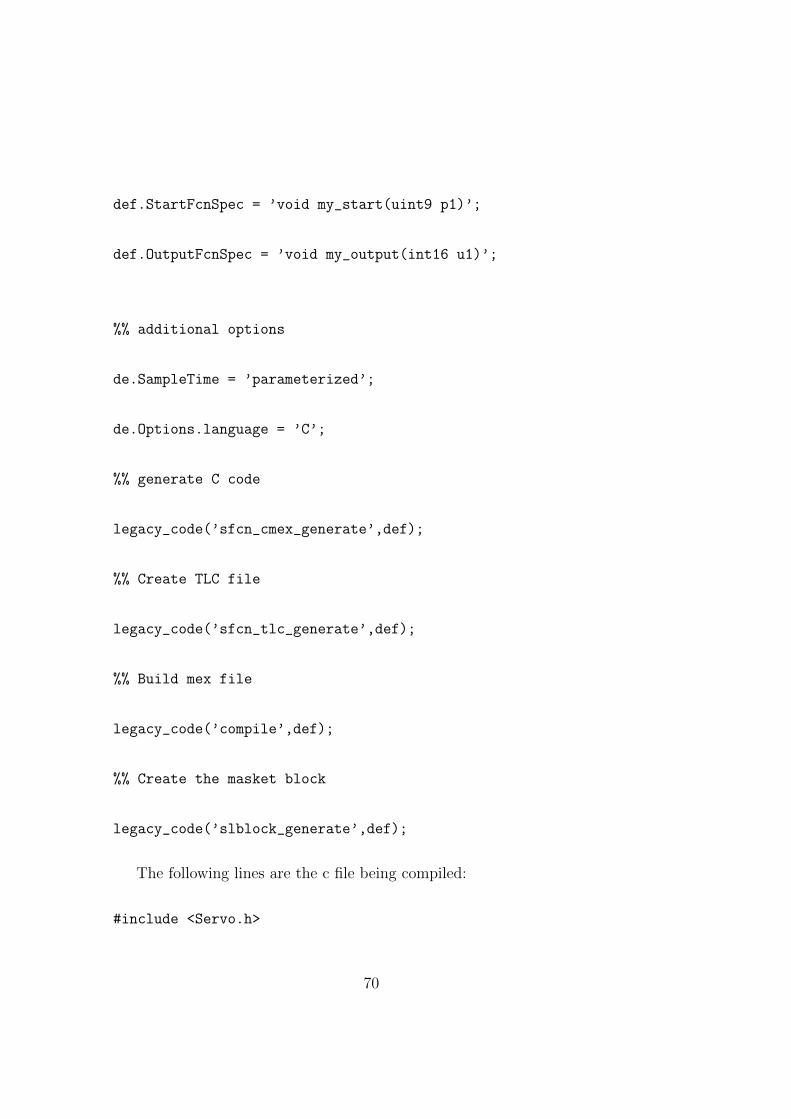
def.StartFcnSpec = ’void my_start(uint9 p1)’;
def.OutputFcnSpec = ’void my_output(int16 u1)’;
%% additional options
de.SampleTime = ’parameterized’;
de.Options.language = ’C’;
%% generate C code
legacy_code(’sfcn_cmex_generate’,def);
%% Create TLC file
legacy_code(’sfcn_tlc_generate’,def);
%% Build mex file
legacy_code(’compile’,def);
%% Create the masket block
legacy_code(’slblock_generate’,def);
The following lines are the c file being compiled:
#include <Servo.h>
70
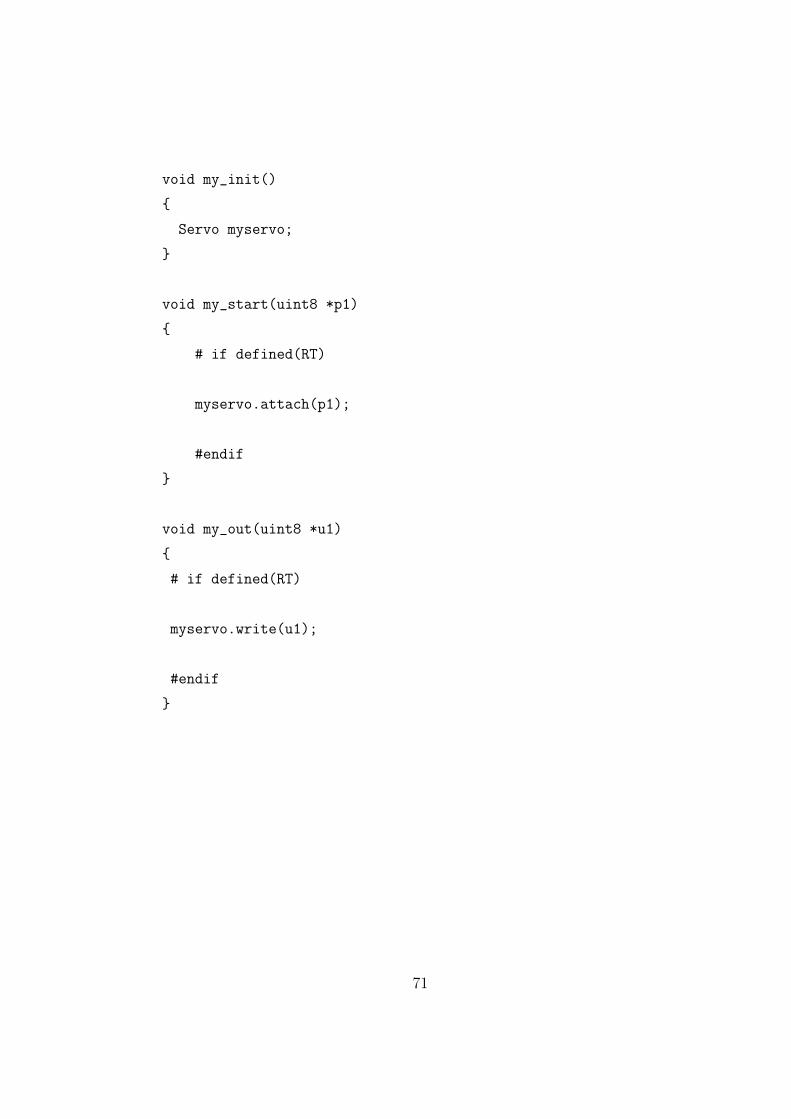
void my_init()
{
Servo myservo;
}
void my_start(uint8 *p1)
{
# if defined(RT)
myservo.attach(p1);
#endif
}
void my_out(uint8 *u1)
{
# if defined(RT)
myservo.write(u1);
#endif
}
71

72
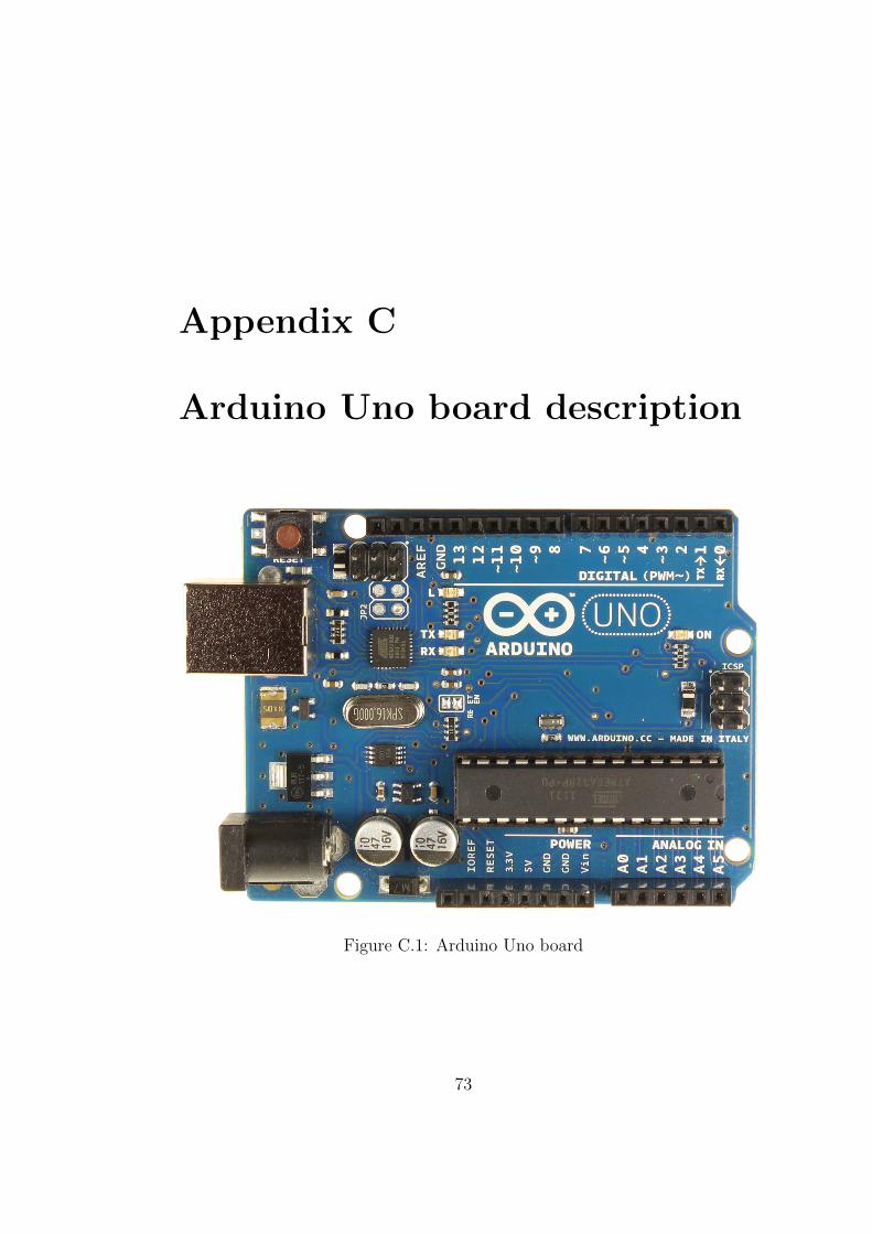
Appendix C
Arduino Uno board description
Figure C.1: Arduino Uno board
73

C.1 Overview
The Arduino Uno is a microcontroller board based on the ATmega328
(datasheet1). It has 14 digital input/output pins (of which 6 can be used
as PWM outputs), 6 analog inputs, a 16 MHz crystal oscillator, a USB
connection, a power jack, an ICSP header, and a reset button. It contains
everything needed to support the microcontroller; simply connect it to a
computer with a USB cable or power it with a AC-to-DC adapter or battery
to get started. Revision 2 of the Uno board has a resistor pulling the 8U2
HWB line to ground, making it easier to put into DFU mode. Revision 3 of
the board has the following new features:
• 1.0 pinout: added SDA and SCL pins that are near to the AREF pin
and two other new pins placed near to the RESET pin, the IOREF
that allow the shields to adapt to the voltage provided from the board.
In future, shields will be compatible both with the board that use the
AVR, which operate with 5V and with the Arduino Due that operate
with 3.3V. The second one is a not connected pin, that is reserved for
future purposes.
• Stronger RESET circuit.
• Atmega 16U2 replace the 8U2.
C.2 Summary
C.3 Power
The Arduino Uno can be powered via the USB connection or with an
external power supply. The power source is selected automatically. External
(non-USB) power can come either from an AC-to-DC adapter (wall-wart) or
battery. The adapter can be connected by plugging a 2.1mm center-positive
1http://www.atmel.com/Images/doc8161.pdf
74
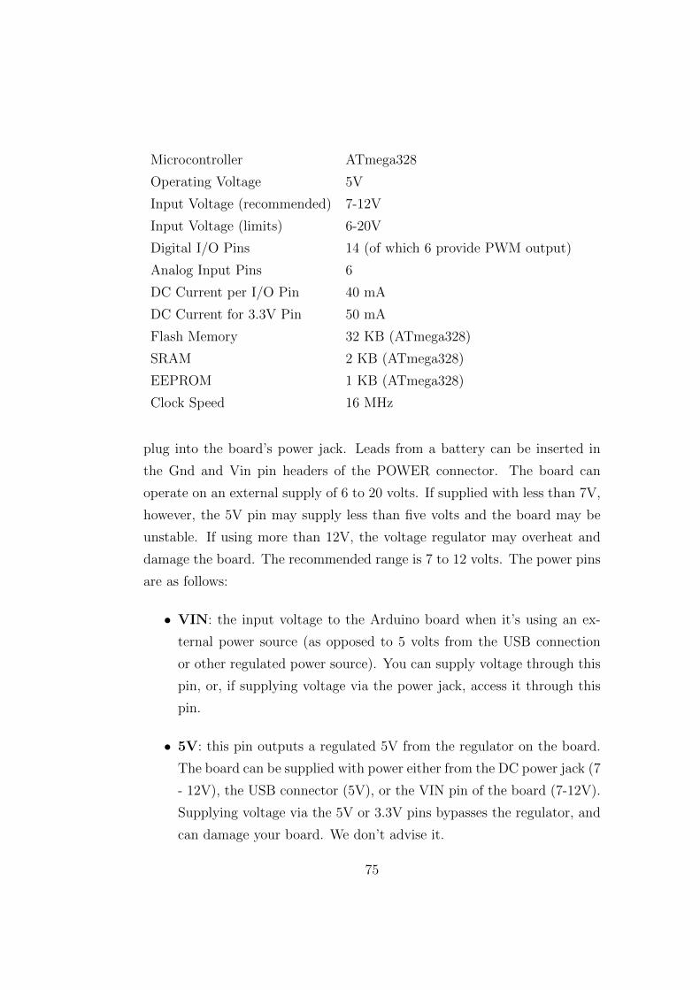
Microcontroller ATmega328
Operating Voltage 5V
Input Voltage (recommended) 7-12V
Input Voltage (limits) 6-20V
Digital I/O Pins 14 (of which 6 provide PWM output)
Analog Input Pins 6
DC Current per I/O Pin 40 mA
DC Current for 3.3V Pin 50 mA
Flash Memory 32 KB (ATmega328)
SRAM 2 KB (ATmega328)
EEPROM 1 KB (ATmega328)
Clock Speed 16 MHz
plug into the board’s power jack. Leads from a battery can be inserted in
the Gnd and Vin pin headers of the POWER connector. The board can
operate on an external supply of 6 to 20 volts. If supplied with less than 7V,
however, the 5V pin may supply less than five volts and the board may be
unstable. If using more than 12V, the voltage regulator may overheat and
damage the board. The recommended range is 7 to 12 volts. The power pins
are as follows:
• VIN: the input voltage to the Arduino board when it’s using an ex-
ternal power source (as opposed to 5 volts from the USB connection
or other regulated power source). You can supply voltage through this
pin, or, if supplying voltage via the power jack, access it through this
pin.
• 5V: this pin outputs a regulated 5V from the regulator on the board.
The board can be supplied with power either from the DC power jack (7
- 12V), the USB connector (5V), or the VIN pin of the board (7-12V).
Supplying voltage via the 5V or 3.3V pins bypasses the regulator, and
can damage your board. We don’t advise it.
75
• 3V3: a 3.3 volt supply generated by the on-board regulator. Maximum
current draw is 50 mA.
• GND: ground pins.
C.4 Input & Output
Each of the 14 digital pins on the Uno can be used as an input or output,
using pinMode(), digitalWrite(), and digitalRead() functions. They operate
at 5 volts. Each pin can provide or receive a maximum of 40 mA and has
an internal pull-up resistor (disconnected by default) of 20-50 kOhms. In
addition, some pins have specialized functions:
• Serial: 0 (RX) and 1 (TX): used to receive (RX) and transmit (TX)
TTL serial data. These pins are connected to the corresponding pins
of the ATmega8U2 USB-to-TTL Serial chip.
• External Interrupts: 2 and 3: these pins can be configured to
trigger an interrupt on a low value, a rising or falling edge, or a change
in value. See the attachInterrupt() function for details.
• PWM: 3, 5, 6, 9, 10, and 11: provide 8-bit PWM output with the
analogWrite() function.
• SPI: 10 (SS), 11 (MOSI), 12 (MISO), 13 (SCK): these pins
support SPI communication using the SPI library.
• LED: 13: there is a built-in LED connected to digital pin 13. When
the pin is HIGH value, the LED is on, when the pin is LOW, it’s off.
The Uno has 6 analog inputs, labeled A0 through A5, each of which
provide 10 bits of resolution (i.e. 1024 different values). By default they
measure from ground to 5 volts, though is it possible to change the upper
end of their range using the AREF pin and the analogReference() function.
Additionally, some pins have specialized functionality:
76

• TWI: A4 or SDA pin and A5 or SCL pin: support TWI com-
munication using the Wire library. There are a couple of other pins on
the board:
• AREF: reference voltage for the analog inputs. Used with analogRef-
erence().
• Reset: bring this line LOW to reset the microcontroller. Typically
used to add a reset button to shields which block the one on the board.
C.5 Communication
The Arduino Uno has a number of facilities for communicating with a
computer, another Arduino, or other microcontrollers. The ATmega328 pro-
vides UART TTL (5V) serial communication, which is available on digital
pins 0 (RX) and 1 (TX). An ATmega16U2 on the board channels this serial
communication over USB and appears as a virtual com port to software on
the computer. The ’16U2 firmware uses the standard USB COM drivers, and
no external driver is needed. However, on Windows, a .inf file is required.
The Arduino software includes a serial monitor which allows simple textual
data to be sent to and from the Arduino board. The RX and TX LEDs on
the board will flash when data is being transmitted via the USB-to-serial
chip and USB connection to the computer (but not for serial communication
on pins 0 and 1). A SoftwareSerial library allows for serial communication
on any of the Uno’s digital pins. The ATmega328 also supports I2C (TWI)
and SPI communication. The Arduino software includes a Wire library to
simplify use of the I2C bus; see the documentation for details. For SPI
communication, use the SPI library.
77

C.6 USB Overcurrent Protection
The Arduino Uno has a resettable polyfuse that protects your computer’s
USB ports from shorts and overcurrent. Although most computers provide
their own internal protection, the fuse provides an extra layer of protection.
If more than 500 mA is applied to the USB port, the fuse will automatically
break the connection until the short or overload is removed.
C.7 Physical Characteristics
The maximum length and width of the Uno PCB are 2.7 and 2.1 inches
respectively, with the USB connector and power jack extending beyond the
former dimension. Four screw holes allow the board to be attached to a
surface or case. Note that the distance between digital pins 7 and 8 is 160
mil (0.16”), not an even multiple of the 100 mil spacing of the other pins.
78
Bibliography
[1] Brian P. Gerkey , Richard T. Vaughan , Andrew Howard. ”The Play-
er/Stage Project: Tools for Multi-Robot and Distributed Sensor Sys-
tems” in text itProceedings of the International Conference on Advanced
Robotics (ICAR 2003) pages 317-323, Coimbra, Portugal, June 30 - July
3, 2003.
[2] Morgan Quigley, Brian Gerkey, Ken Conley, Josh Faust, Tully Foote,
Jeremy Leibs, Eric Berger, Rob Wheeler, Andrew Ng. ”ROS: an open-
source Robot Operating System” . 2008
[3] Anirban Basumallik ”Survey of Robot Programming Languages”, sem-
inar Report. Bombay, April 2010
[4] Walter Miani, Andre Araujo , Micael Couceiro, David Portugal, Rui P.
Rocha ”StingBot Technical Manual”, Coimbra, May 2012
[5] MathWorks - MATLAB and Simulink for Technical Computing,
http://www.mathworks.it/, May 2012
[6] Phyton Robotics, http://pyrorobotics.org/, May 2012
[7] Wikipedia - Phyton, http://it.wikipedia.org/wiki/Python, May 2012
[8] Skilligent, http://www.skilligent.com/, May 2012
[9] Stinger Robot Kit, http://www.roboticsconnection.com/p-73-stinger-
robot-kit.aspx, April 2012
79

[10] Arduino, http://www.arduino.cc/, September 2012
[11] Giampiero Campa, ”Learning Basic Mechatronics concepts using the
Arduino Board and MATLAB”, 2011
[12] Michael Margolis, ”Arduino Cookbook”, March 2011
80