The dynamic range of burstingin a network of

respiratory pacemaker cells

Alla Borisyuk

Universityof Utah

Joint work with:

Janet BestJonathan RubinDavid Terman

Martin Wechselberger

Mathematical Biosciences Institute (MBI), OSU

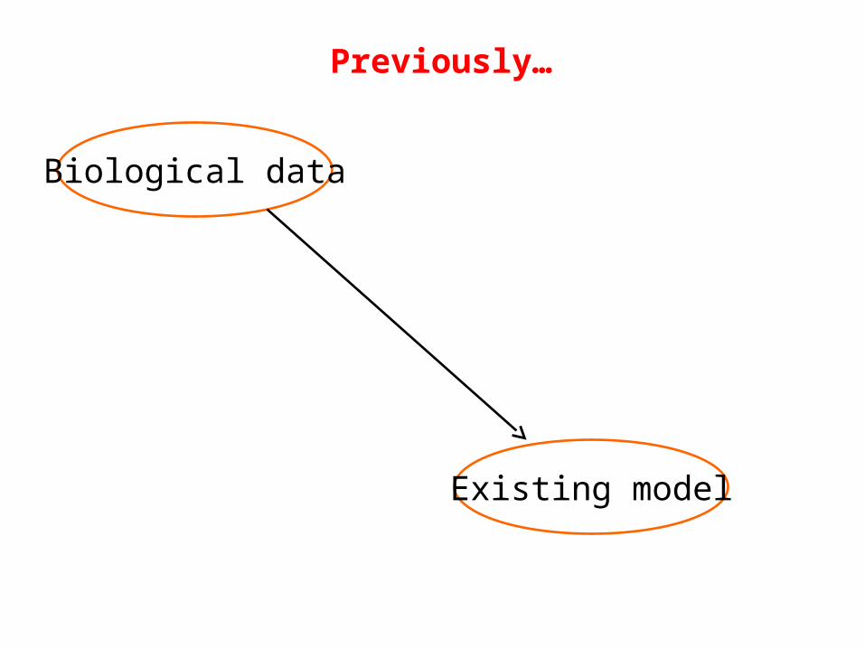
Biological data

Existing model

Previously…

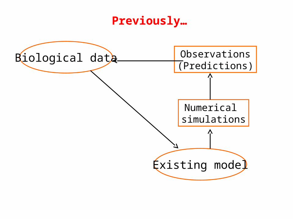
Biological data

Existing model

Numerical simulations

Observations(Predictions)

Previously…

Biological data

Existing model

Numerical simulations

Observations(Predictions)

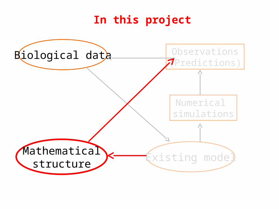
In this project

Mathematicalstructure

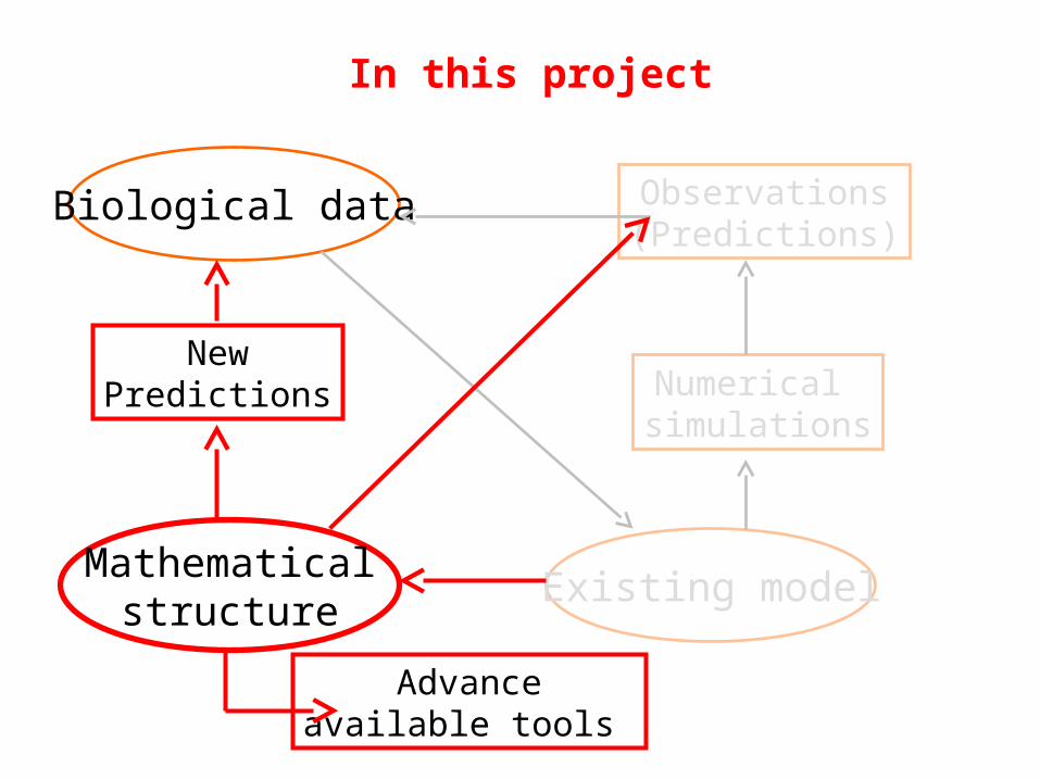
Biological data

Existing model

Numerical simulations

Observations(Predictions)

In this project

Mathematicalstructure

Advanceavailable tools

NewPredictions

Motivation: analyze model for neuronal activity in the Pre-Bötzinger complex

Control of respiratory rhythm originates in this area

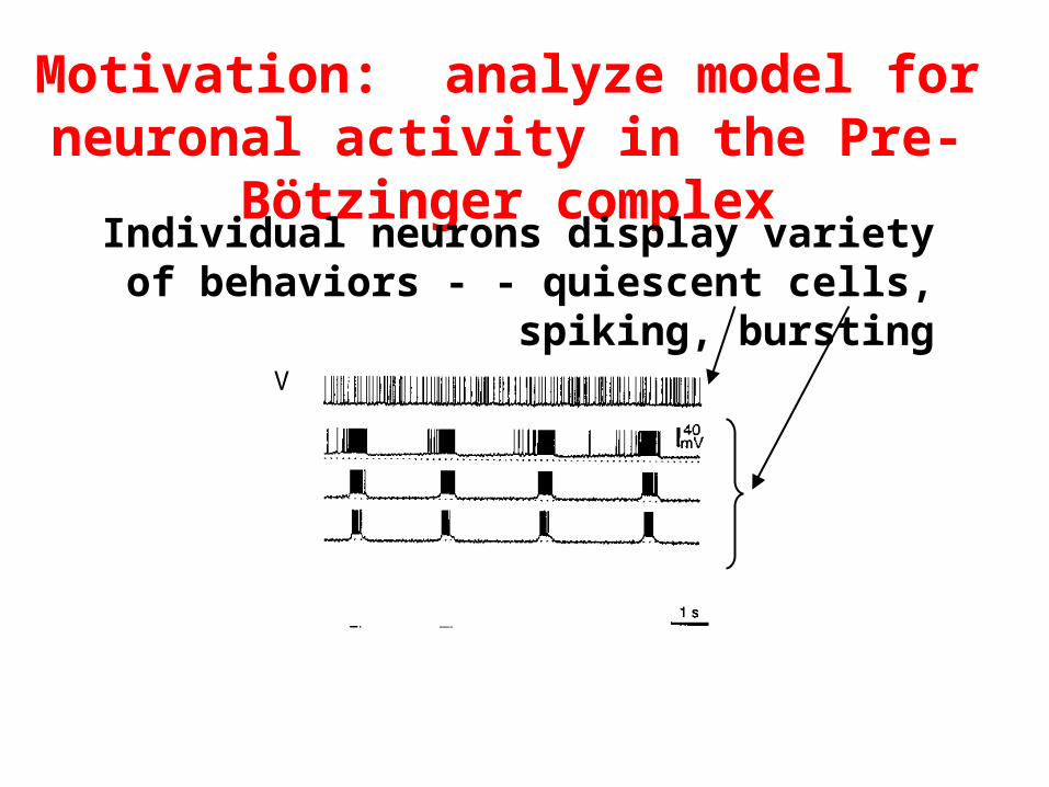
Motivation: analyze model for neuronal activity in the Pre-Bötzinger complex

Individual neurons display variety of behaviors - - quiescent cells, spiking, bursting

V

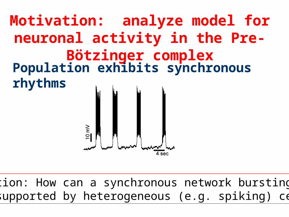
Motivation: analyze model for neuronal activity in the Pre-Bötzinger complex

Population exhibits synchronous rhythms

figure

Question: How can a synchronous network bursting be supported by heterogeneous (e.g. spiking) cells?

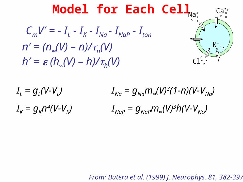
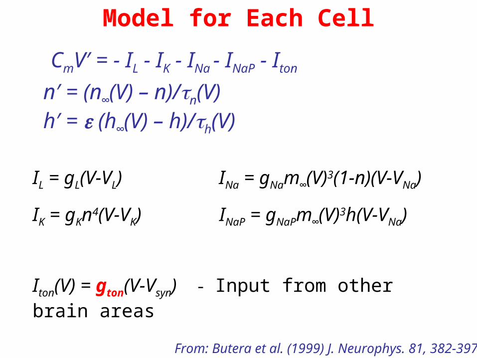
Model for Each Cell

IL = gL(V-VL) INa = gNam∞(V)3(1-n)(V-VNa)

IK = gKn4(V-VK) INaP = gNaPm∞(V)3h(V-VNa)

n′ = (n∞(V) – n)/n(V)h′ = (h∞(V) – h)/h(V)

CmV′ = - IL - IK - INa - INaP - Iton

From: Butera et al. (1999) J. Neurophys. 81, 382-397

Na+ Ca2+

K+

Cl-

Model for Each Cell

IL = gL(V-VL) INa = gNam∞(V)3(1-n)(V-VNa)

IK = gKn4(V-VK) INaP = gNaPm∞(V)3h(V-VNa)

Iton(V) = gton(V-Vsyn) - Input from other brain areas

n′ = (n∞(V) – n)/n(V)h′ = (h∞(V) – h)/h(V)

CmV′ = - IL - IK - INa - INaP - Iton

From: Butera et al. (1999) J. Neurophys. 81, 382-397

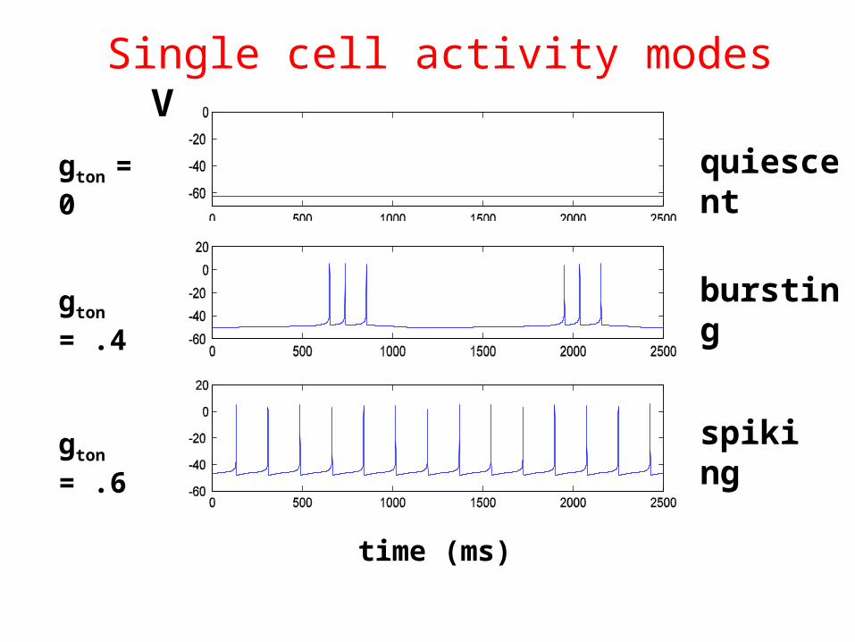
V

time (ms)

quiescent

bursting

spiking

gton = 0

gton = .4

gton = .6

Single cell activity modes

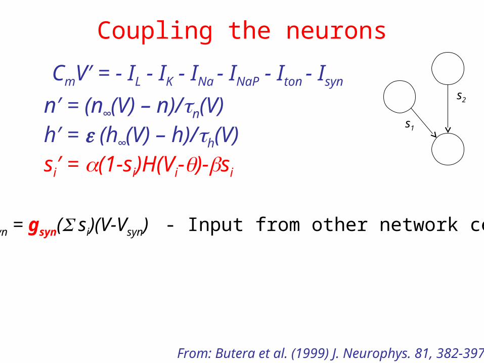
n′ = (n∞(V) – n)/n(V)h′ = (h∞(V) – h)/h(V)si′ = (1-si)H(Vi-)-si

CmV′ = - IL - IK - INa - INaP - Iton - Isyn

Coupling the neurons

Isyn = gsyn( si)(V-Vsyn) - Input from other network cells

From: Butera et al. (1999) J. Neurophys. 81, 382-397

s1

s2

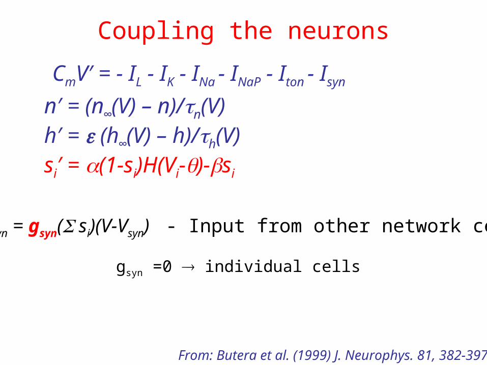
n′ = (n∞(V) – n)/n(V)h′ = (h∞(V) – h)/h(V)si′ = (1-si)H(Vi-)-si

CmV′ = - IL - IK - INa - INaP - Iton - Isyn

Coupling the neurons

From: Butera et al. (1999) J. Neurophys. 81, 382-397

gsyn =0 individual cells

Isyn = gsyn( si)(V-Vsyn) - Input from other network cells

n′ = (n∞(V) – n)/n(V)h′ = (h∞(V) – h)/h(V)si′ = (1-si)H(Vi-)-si

CmV′ = - IL - IK - INa - INaP - Iton - Isyn

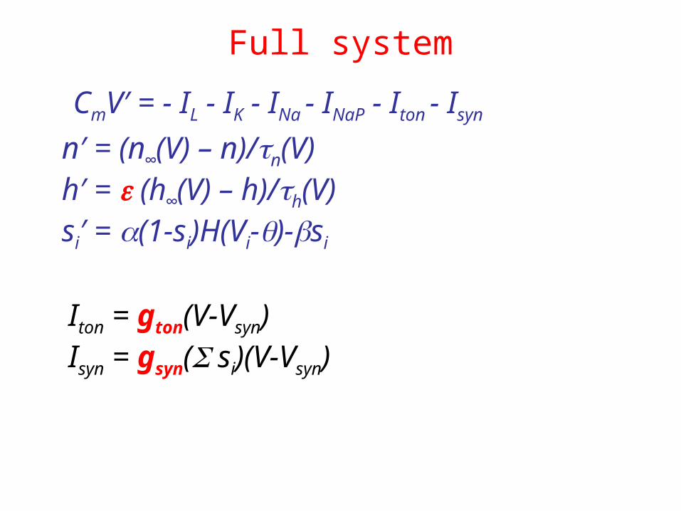
Full system

Iton = gton(V-Vsyn) Isyn = gsyn( si)(V-Vsyn)

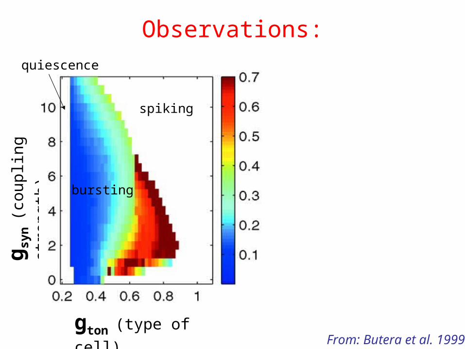
Observations:

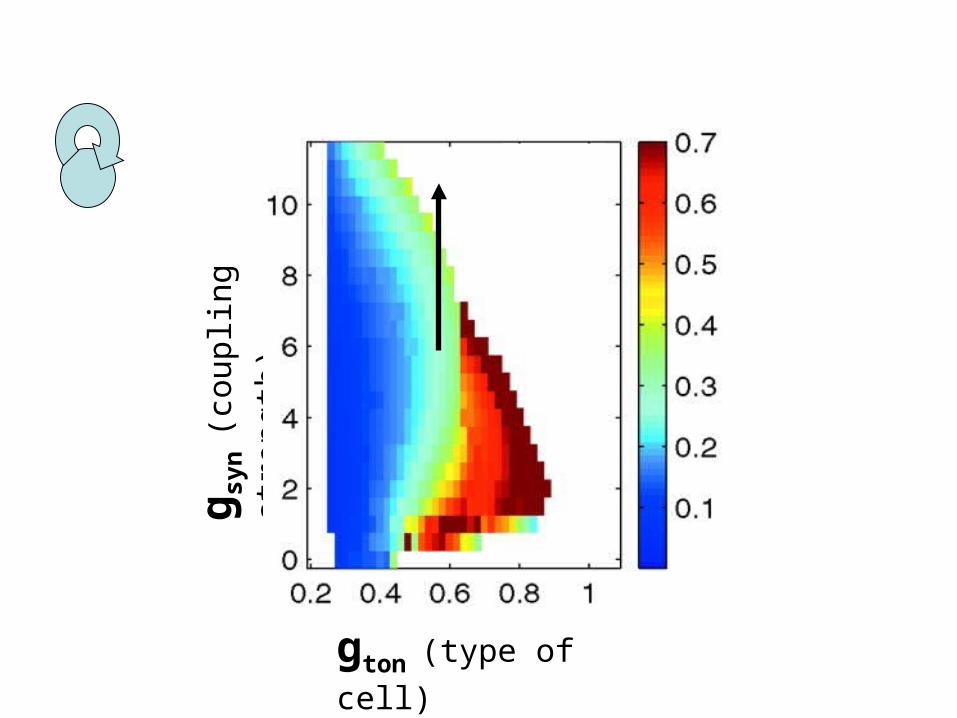
gton (type of cell)

g syn

(cou

plin

g st

reng

th)

bursting

spiking

quiescence

From: Butera et al. 1999

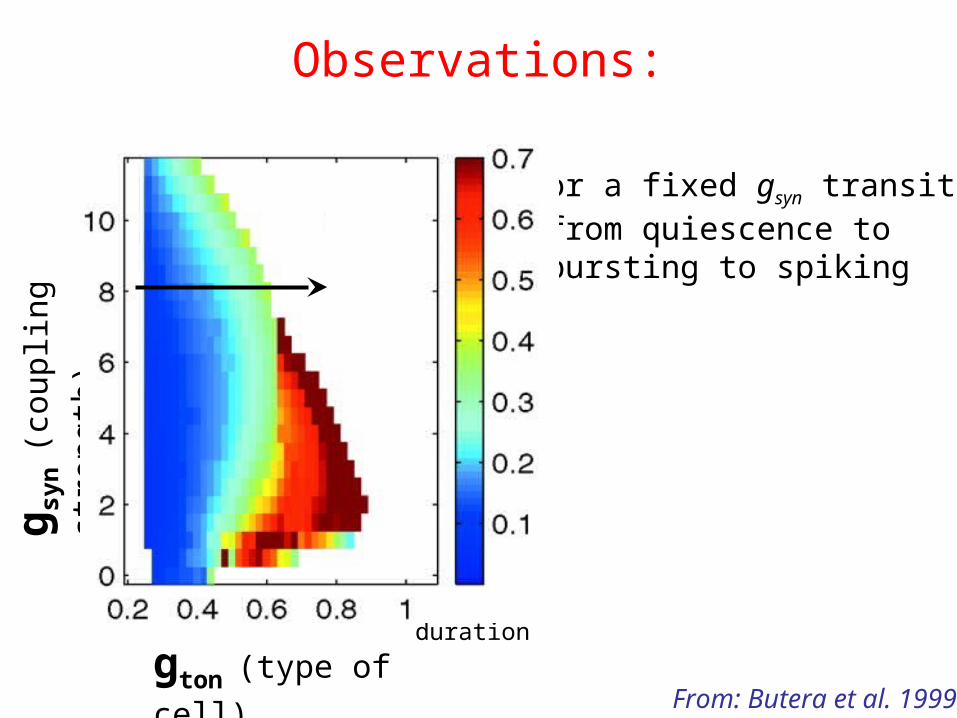
Observations:

gton (type of cell)

g syn

(cou

plin

g st

reng

th)

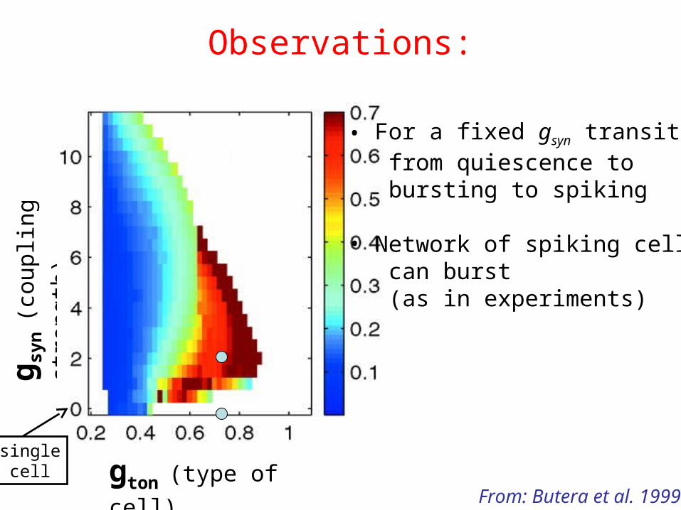
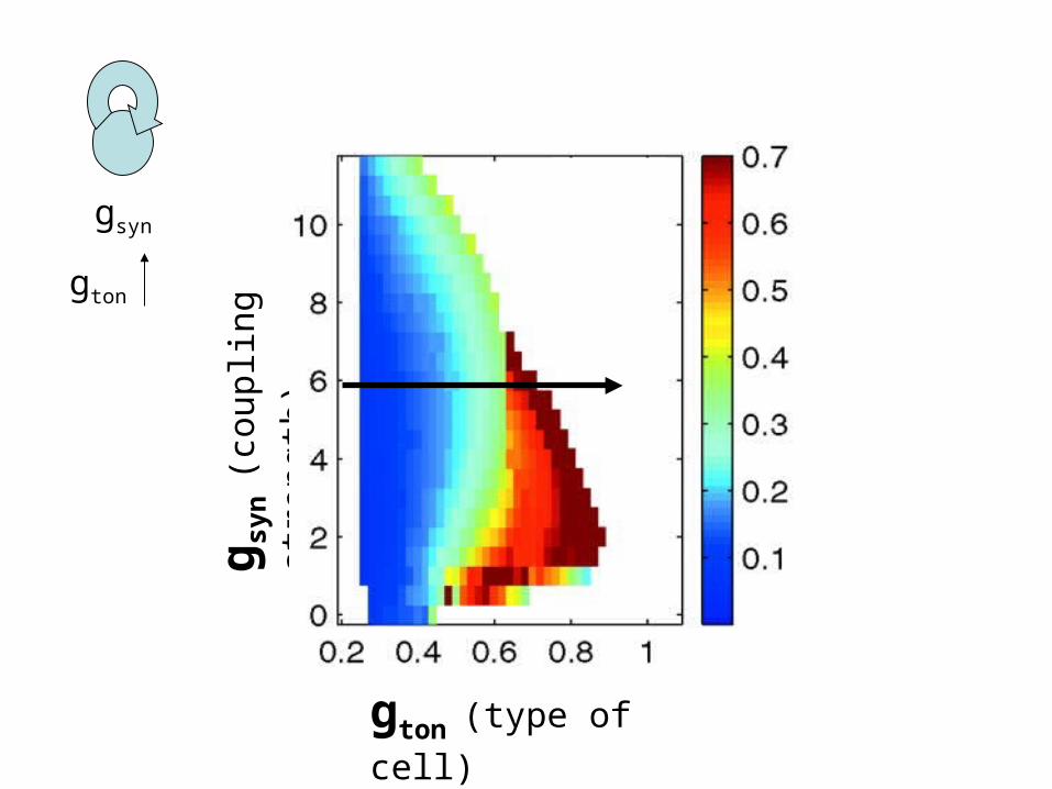
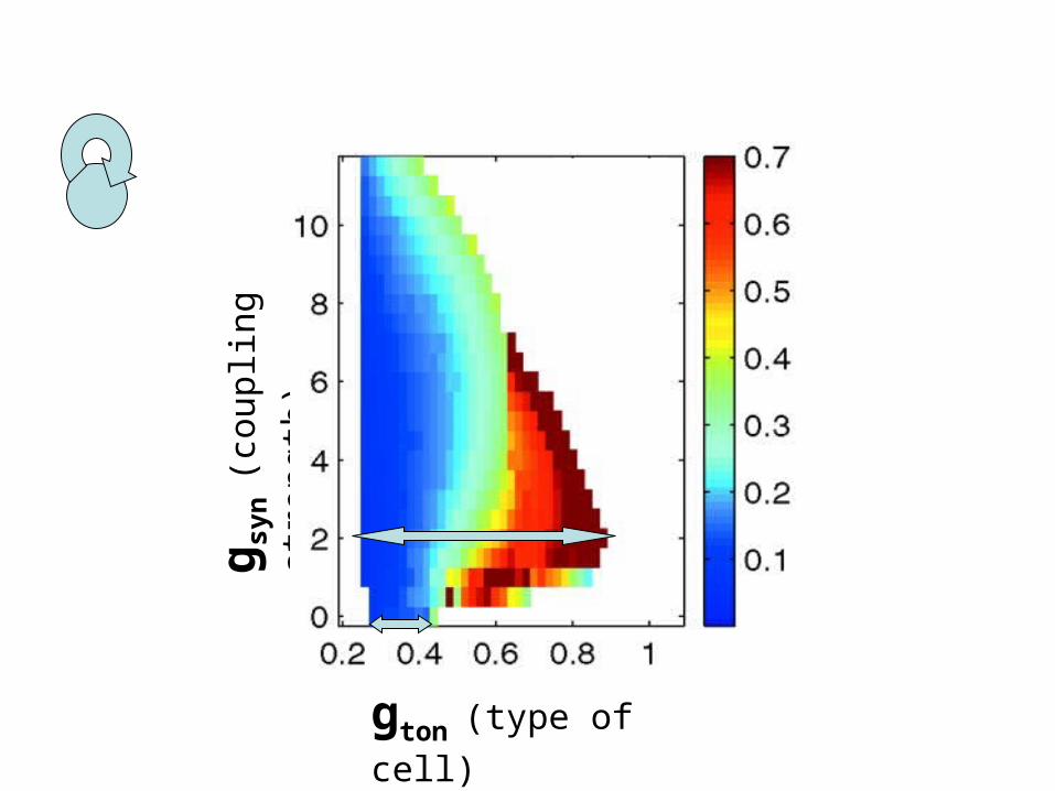
• For a fixed gsyn transitions from quiescence to bursting to spiking

Burstduration

From: Butera et al. 1999

Observations:

gton (type of cell)

g syn

(cou

plin

g st

reng

th)

From: Butera et al. 1999

• For a fixed gsyn transitions from quiescence to bursting to spiking

• Network of spiking cells can burst (as in experiments)

singlecell

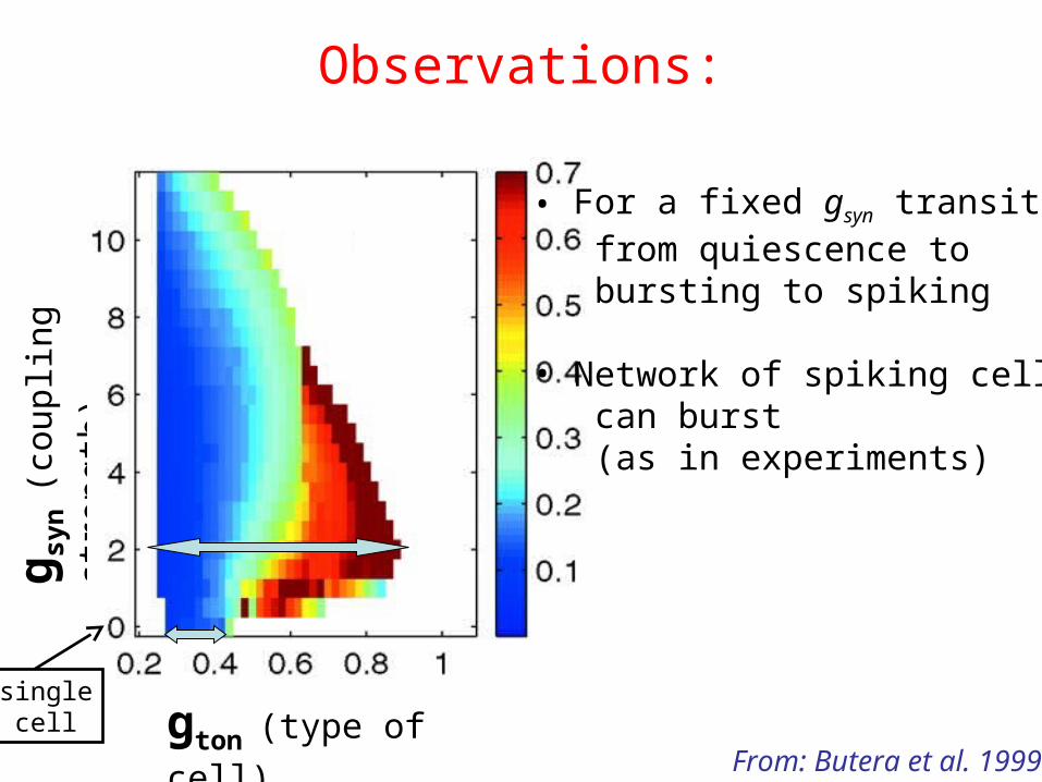
Observations:

gton (type of cell)

g syn

(cou

plin

g st

reng

th)

From: Butera et al. 1999

• For a fixed gsyn transitions from quiescence to bursting to spiking

• Network of spiking cells can burst (as in experiments)

singlecell

Observations:

gton (type of cell)

g syn

(cou

plin

g st

reng

th)

Burstduration

From: Butera et al. 1999

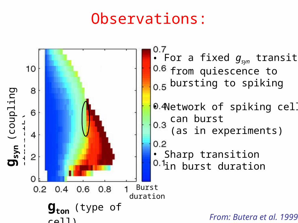
• For a fixed gsyn transitions from quiescence to bursting to spiking

• Network of spiking cells can burst (as in experiments)

• Sharp transition in burst duration

Observations:

gton (type of cell)

g syn

(cou

plin

g st

reng

th)

From: Butera et al. 1999

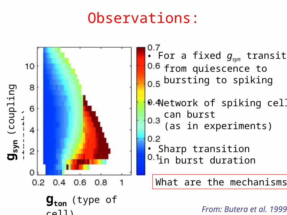
What are the mechanisms?

• For a fixed gsyn transitions from quiescence to bursting to spiking

• Network of spiking cells can burst (as in experiments)

• Sharp transition in burst duration

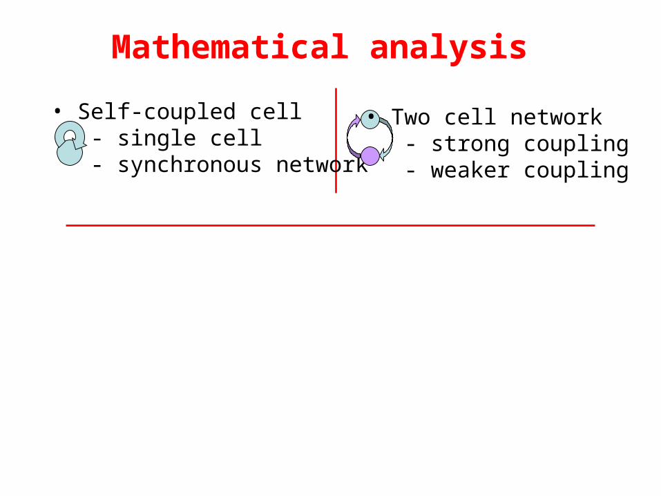
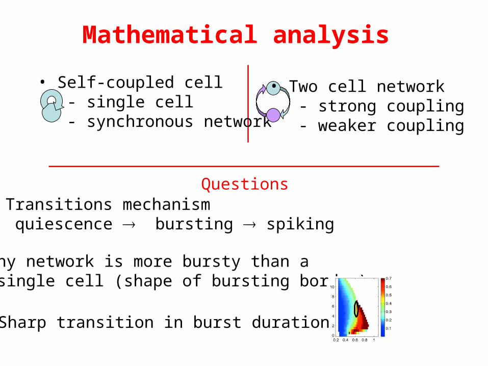
Mathematical analysis

• Self-coupled cell - single cell - synchronous network

• Two cell network - strong coupling - weaker coupling

Mathematical analysis

• Self-coupled cell - single cell - synchronous network

• Two cell network - strong coupling - weaker coupling

• Transitions mechanism quiescence bursting spiking

Questions

• Why network is more bursty than a single cell (shape of bursting border)

• Sharp transition in burst duration

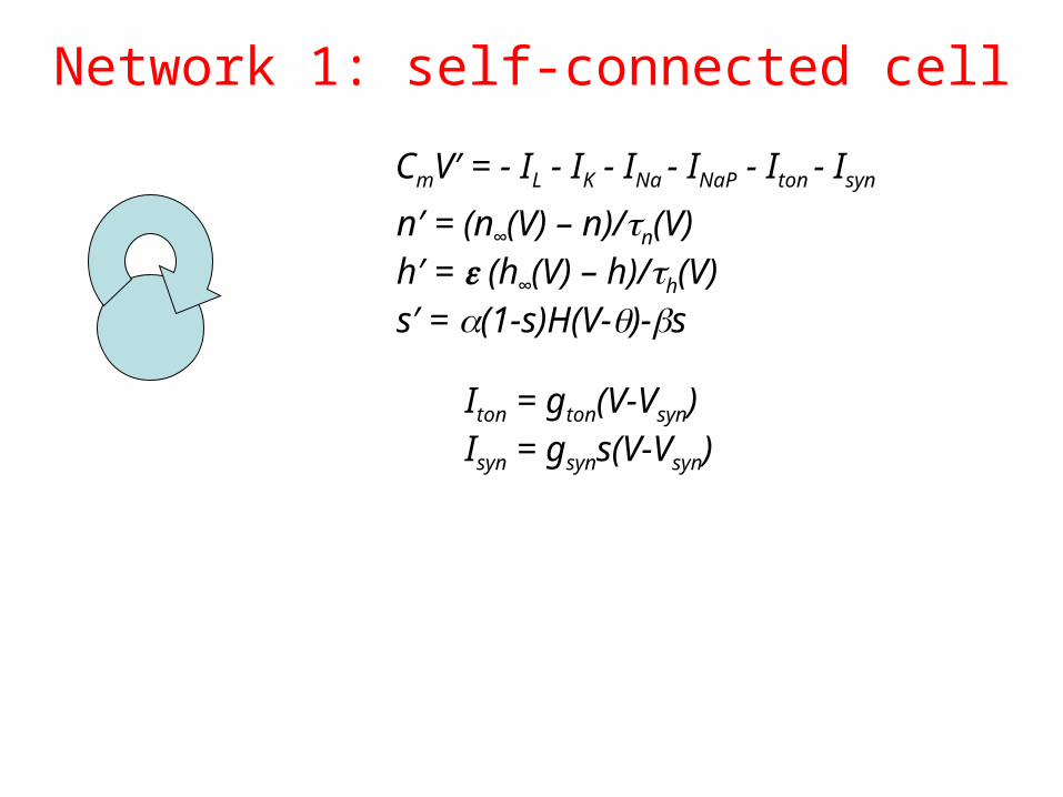
Network 1: self-connected cell

n′ = (n∞(V) – n)/n(V)h′ = (h∞(V) – h)/h(V)s′ = (1-s)H(V-)-s

CmV′ = - IL - IK - INa - INaP - Iton - Isyn

Iton = gton(V-Vsyn) Isyn = gsyns(V-Vsyn)

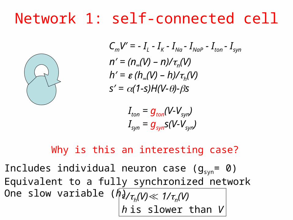
Network 1: self-connected cell

n′ = (n∞(V) – n)/n(V)h′ = (h∞(V) – h)/h(V)s′ = (1-s)H(V-)-s

CmV′ = - IL - IK - INa - INaP - Iton - Isyn

Iton = gton(V-Vsyn) Isyn = gsyns(V-Vsyn)

Why is this an interesting case?

• Includes individual neuron case (gsyn= 0)• Equivalent to a fully synchronized network• One slow variable (h) /h(V) ≪ 1/n(V)

h is slower than V

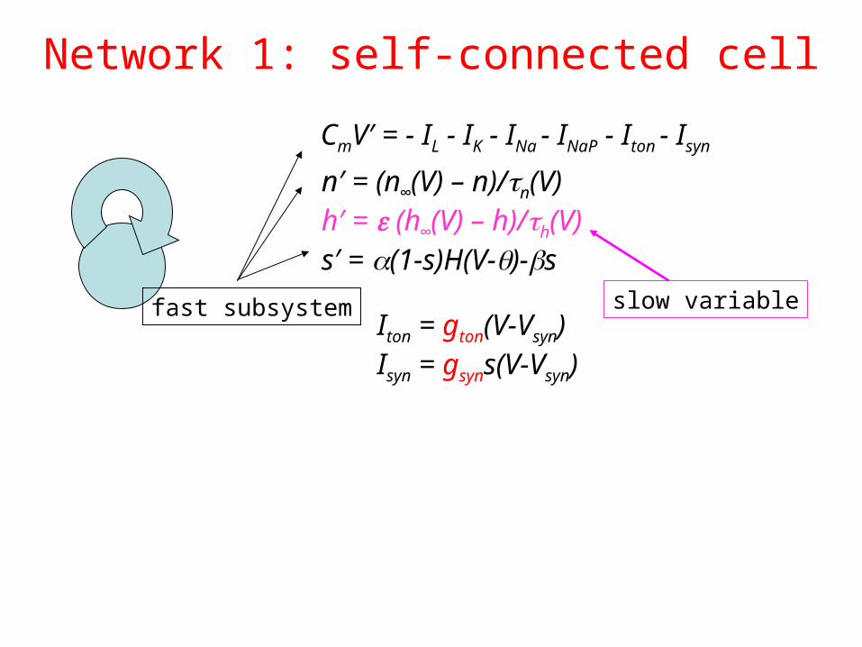
Network 1: self-connected cell

n′ = (n∞(V) – n)/n(V)h′ = (h∞(V) – h)/h(V)s′ = (1-s)H(V-)-s

CmV′ = - IL - IK - INa - INaP - Iton - Isyn

Iton = gton(V-Vsyn) Isyn = gsyns(V-Vsyn)

fast subsystem slow variable

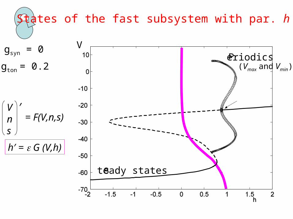
gsyn = 0

States of the fast subsystem with par. h

gton = 0.2

V

teady states

eriodics(Vmax and Vmin)

Vns

′= F(V,n,s)

h′ = G (V,h)

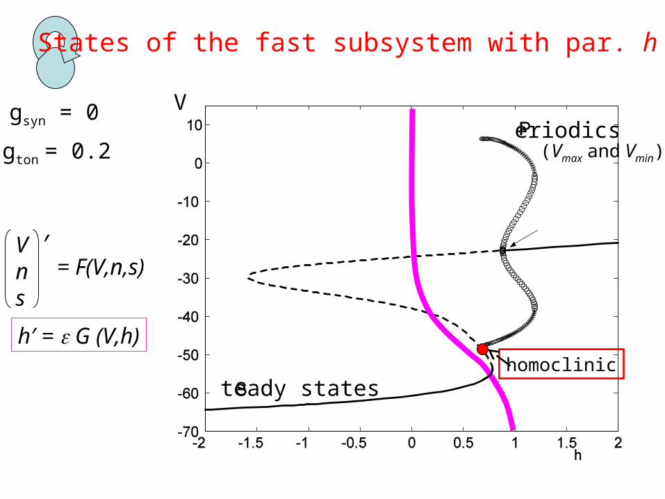
gsyn = 0

States of the fast subsystem with par. h

gton = 0.2

V

teady states

eriodics(Vmax and Vmin)

Vns

′= F(V,n,s)

h′ = G (V,h)homoclinic

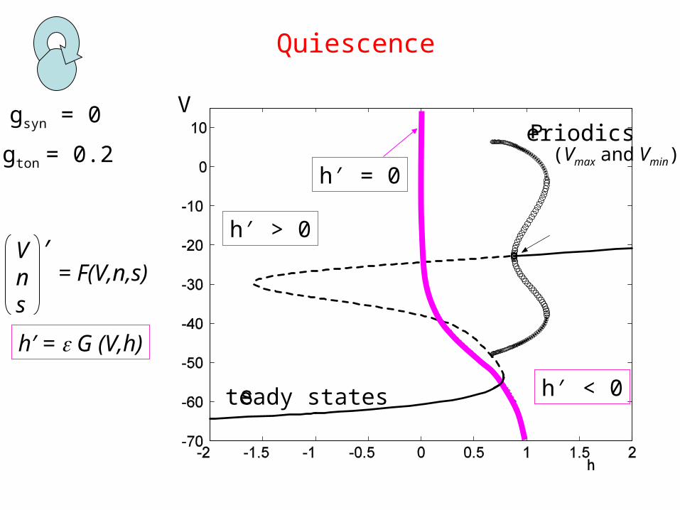
gsyn = 0

Quiescence

gton = 0.2

V

teady states

eriodics

h′ = 0

h′ < 0

h′ > 0

(Vmax and Vmin)

Vns

′= F(V,n,s)

h′ = G (V,h)

gton (type of cell)

g syn

(cou

plin

g st

reng

th)

gsyn

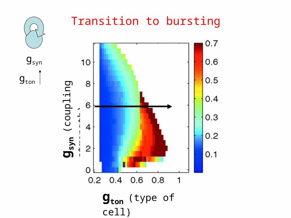
Transition to bursting

gton

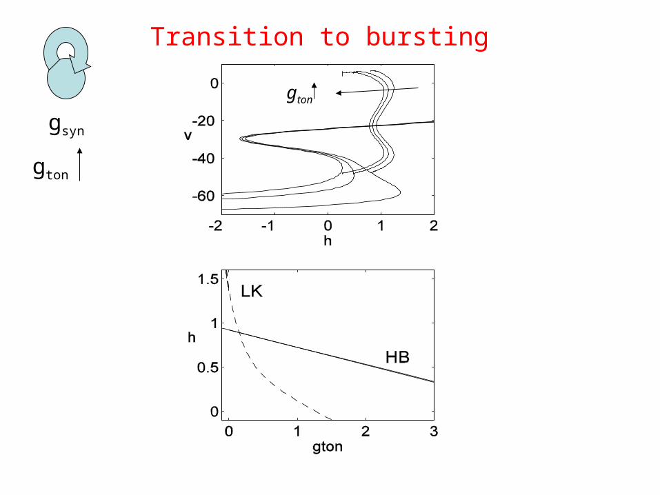
gsyn

gton

Transition to bursting

gton

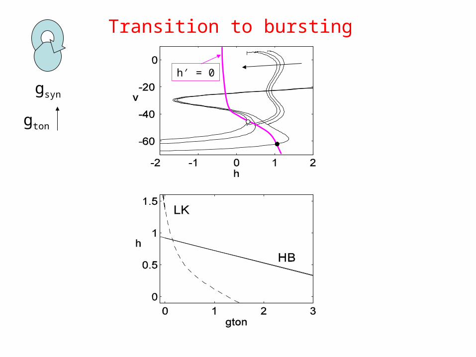
gsyn

h′ = 0

gton

Transition to bursting

gsyn

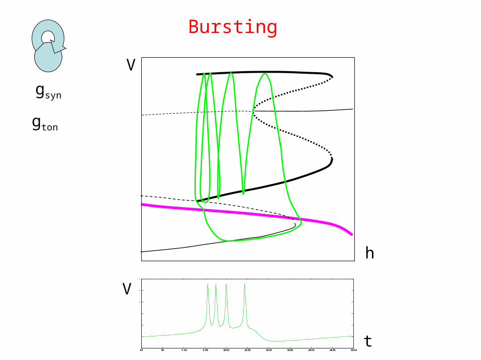
h

V

Bursting

gton

t

V

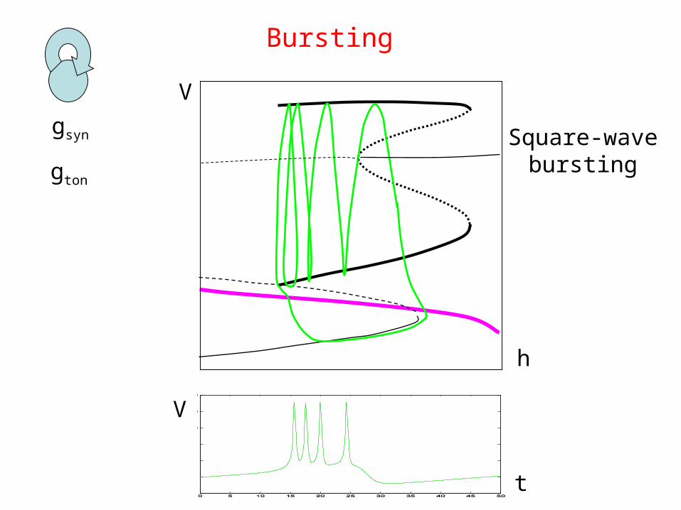
gsyn

h

V

Bursting

gton

t

V

Square-wavebursting

gton (type of cell)

g syn

(cou

plin

g st

reng

th)

gsyn

gton

gsyn

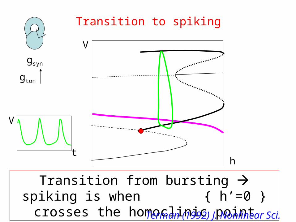
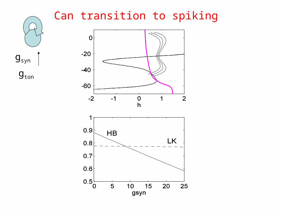
Transition to spiking

gton

h

V

Transition from bursting spiking is when { h’=0 } crosses the homoclinic point

t

V

Terman (1992) J. Nonlinear Sci.

gton (type of cell)

g syn

(cou

plin

g st

reng

th)

gsyn

gton

gton (type of cell)

g syn

(cou

plin

g st

reng

th)

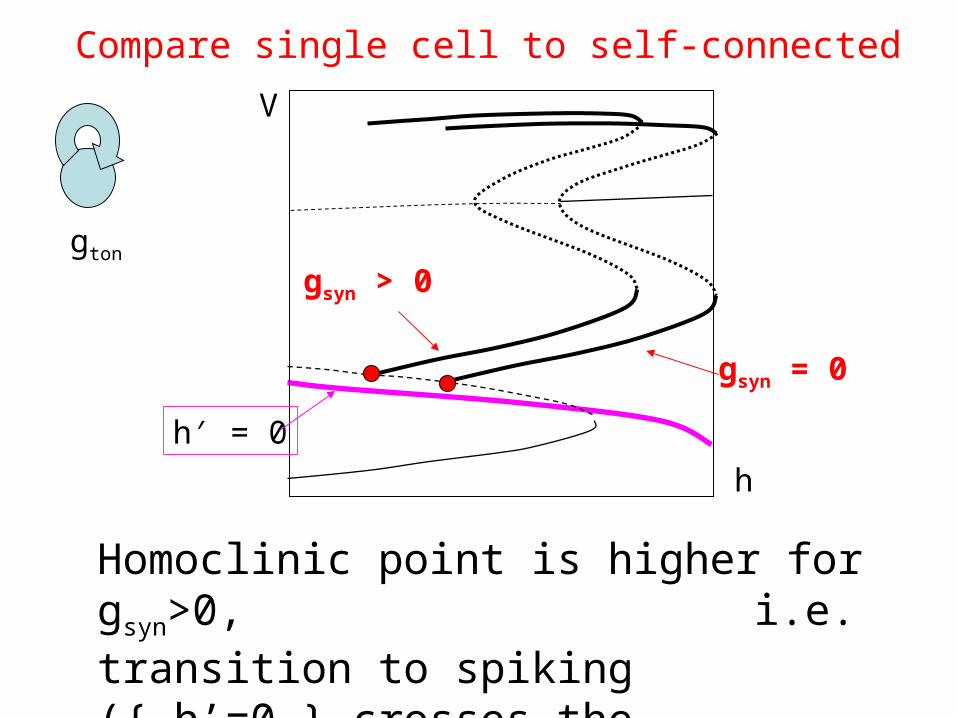
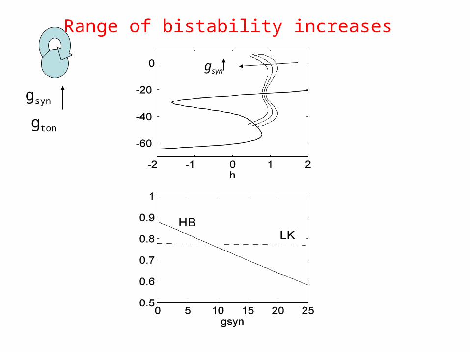
Compare single cell to self-connected

gton

h

V

gsyn = 0

gsyn > 0

h′ = 0

Homoclinic point is higher for gsyn>0, i.e. transition to spiking ({ h’=0 } crosses the homoclinic point) will happen for larger gton

gton (type of cell)

g syn

(cou

plin

g st

reng

th)

This explains wider range of bursting

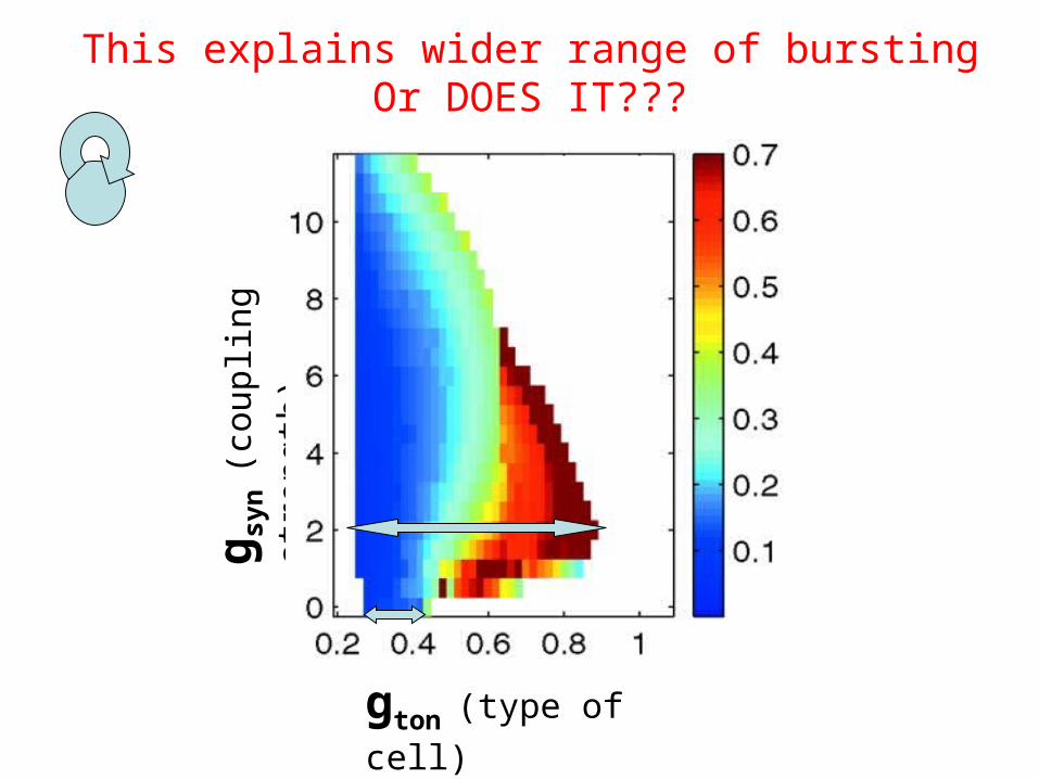
gton (type of cell)

g syn

(cou

plin

g st

reng

th)

This explains wider range of burstingOr DOES IT???

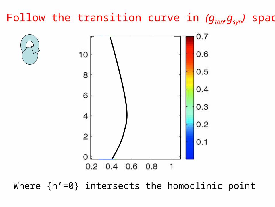
Follow the transition curve in (gton,gsyn) space

Where {h’=0} intersects the homoclinic point

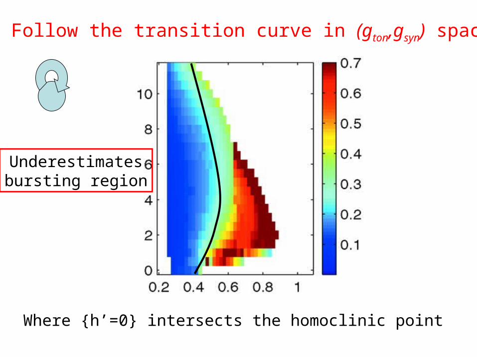
Follow the transition curve in (gton,gsyn) space

Where {h’=0} intersects the homoclinic point

Underestimatesbursting region

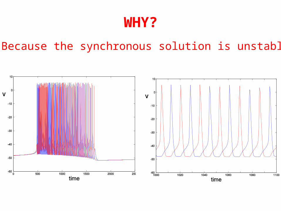
WHY?

Because the synchronous solution is unstable

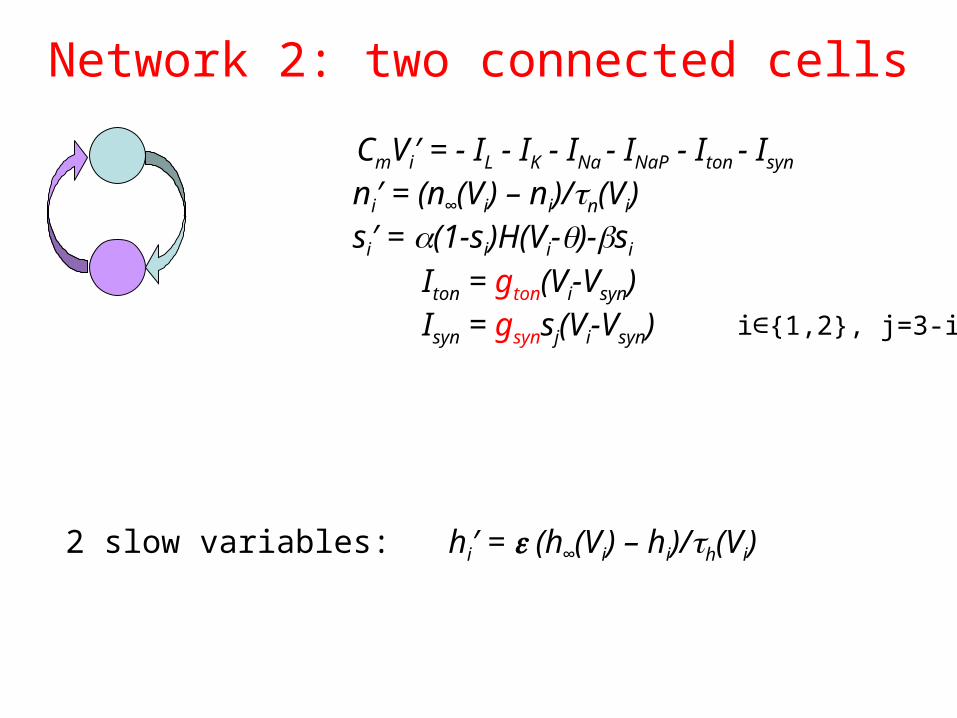
Network 2: two connected cells

ni′ = (n∞(Vi) – ni)/n(Vi)si′ = (1-si)H(Vi-)-si

2 slow variables: hi′ = (h∞(Vi) – hi)/h(Vi)

CmVi′ = - IL - IK - INa - INaP - Iton - Isyn

Iton = gton(Vi-Vsyn) Isyn = gsynsj(Vi-Vsyn) i∈{1,2}, j=3-i

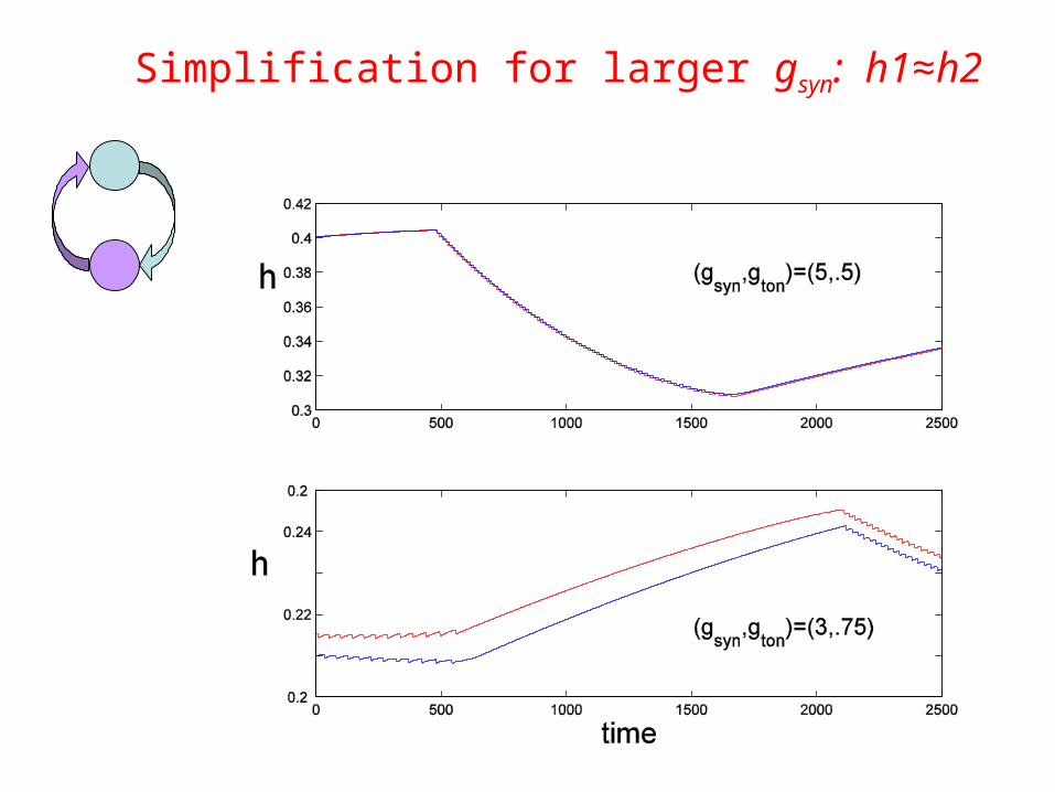
Simplification for larger gsyn: h1≈h2

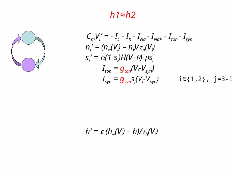
ni′ = (n∞(Vi) – ni)/n(Vi)si′ = (1-si)H(Vi-)-si

h′ = (h∞(Vi) – h)/h(Vi)

CmVi′ = - IL - IK - INa - INaP - Iton - Isyn

Iton = gton(Vi-Vsyn) Isyn = gsynsj(Vi-Vsyn) i∈{1,2}, j=3-i

h1≈h2

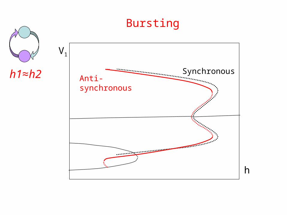
SynchronousAnti-synchronous

h

V1

Bursting

h1≈h2

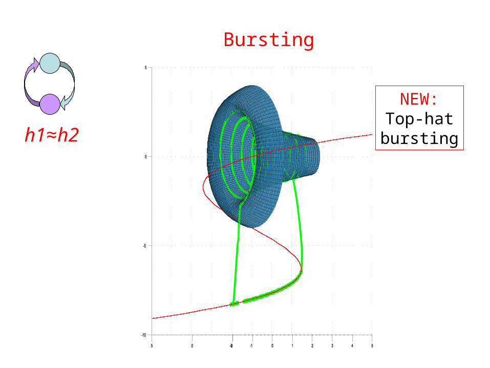
Bursting

h1≈h2

NEW:Top-hatbursting

Features of top-hat bursting:

h1≈h2

• Square wave bursters, when coupled, can generate top hat bursting

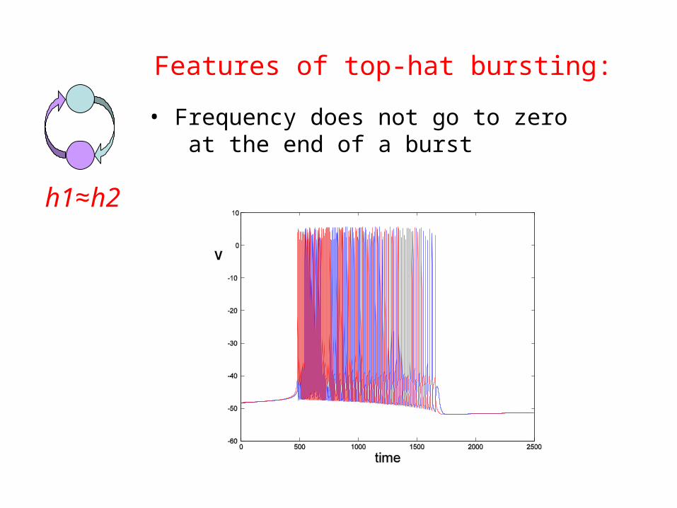
Features of top-hat bursting:

h1≈h2

• Frequency does not go to zero at the end of a burst

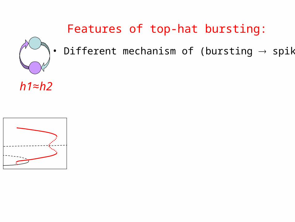
Features of top-hat bursting:

h1≈h2

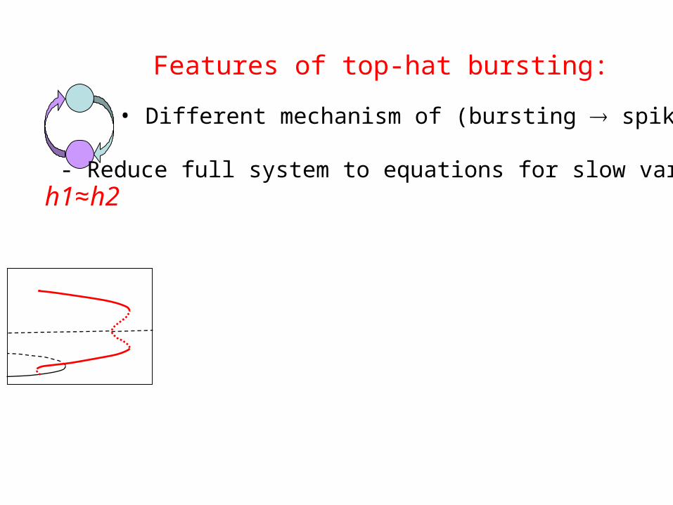
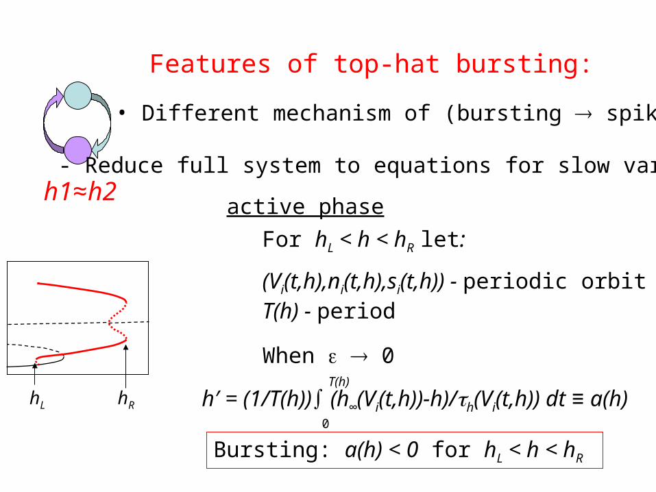
• Different mechanism of (bursting spiking)

Features of top-hat bursting:

h1≈h2

• Different mechanism of (bursting spiking)

- Reduce full system to equations for slow variables:

Features of top-hat bursting:

h1≈h2

• Different mechanism of (bursting spiking)

- Reduce full system to equations for slow variables:

active phase

hL hR

For hL < h < hR let:

(Vi(t,h),ni(t,h),si(t,h)) - periodic orbitT(h) - period

When 0

h′ = (1/T(h))∫ (h∞(Vi(t,h))-h)/h(Vi(t,h)) dt ≡ a(h)0

T(h)

Bursting: a(h) < 0 for hL < h < hR

Features of top-hat bursting:

h1≈h2

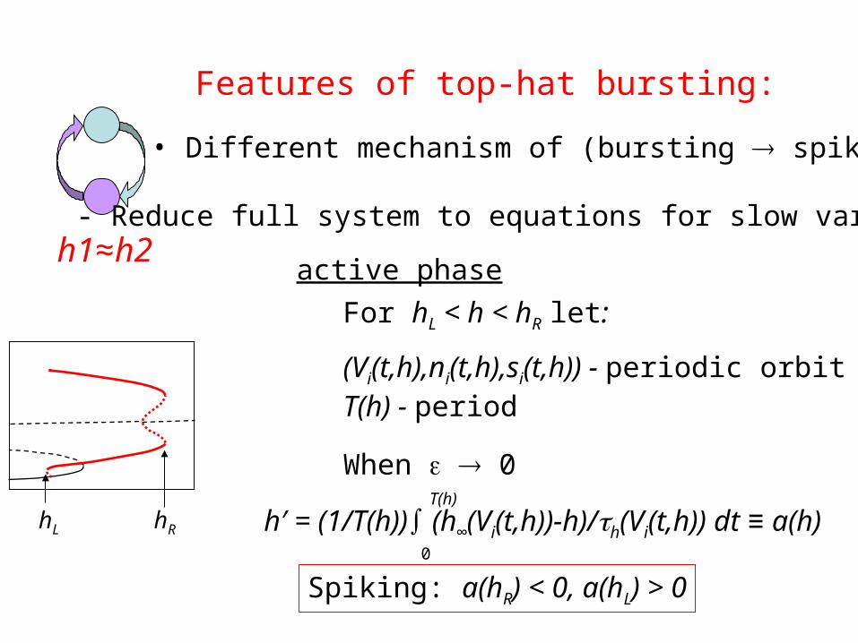
• Different mechanism of (bursting spiking)

- Reduce full system to equations for slow variables:

active phase

hL hR

For hL < h < hR let:

(Vi(t,h),ni(t,h),si(t,h)) - periodic orbitT(h) - period

When 0

h′ = (1/T(h))∫ (h∞(Vi(t,h))-h)/h(Vi(t,h)) dt ≡ a(h)0

T(h)

Spiking: a(hR) < 0, a(hL) > 0

Features of top-hat bursting:

h1≈h2

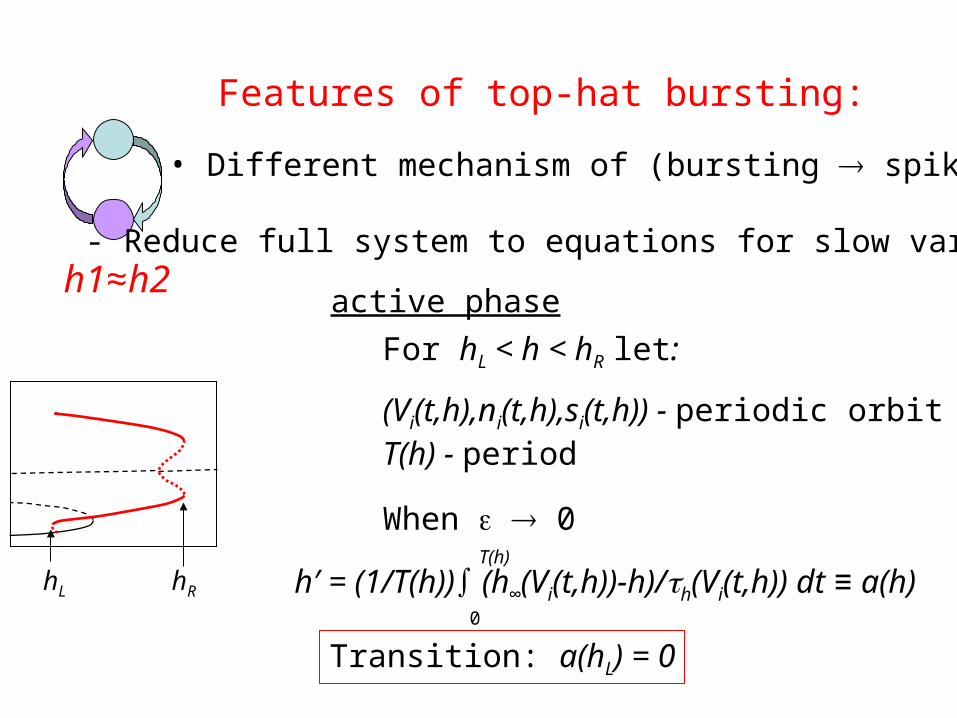
• Different mechanism of (bursting spiking)

- Reduce full system to equations for slow variables:

active phase

hL hR

For hL < h < hR let:

(Vi(t,h),ni(t,h),si(t,h)) - periodic orbitT(h) - period

When 0

h′ = (1/T(h))∫ (h∞(Vi(t,h))-h)/h(Vi(t,h)) dt ≡ a(h)0

T(h)

Transition: a(hL) = 0

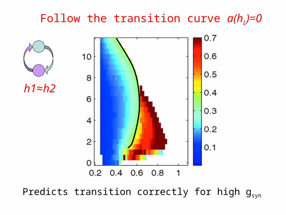
Follow the transition curve a(hL)=0

Predicts transition correctly for high gsyn

h1≈h2

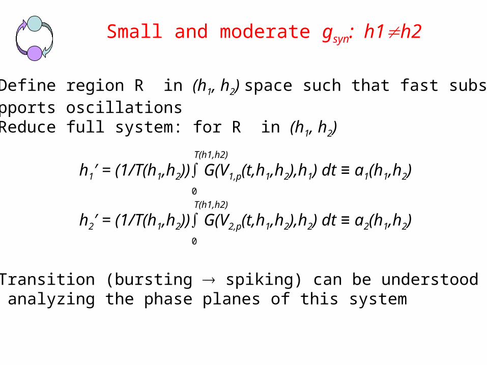
Small and moderate gsyn: h1h2

• Define region R in (h1, h2) space such that fast subsystemsupports oscillations• Reduce full system: for R in (h1, h2)

• Transition (bursting spiking) can be understood by analyzing the phase planes of this system

h1′ = (1/T(h1,h2))∫ G(V1,p(t,h1,h2),h1) dt ≡ a1(h1,h2)0

T(h1,h2)

h2′ = (1/T(h1,h2))∫ G(V2,p(t,h1,h2),h2) dt ≡ a2(h1,h2)0

T(h1,h2)

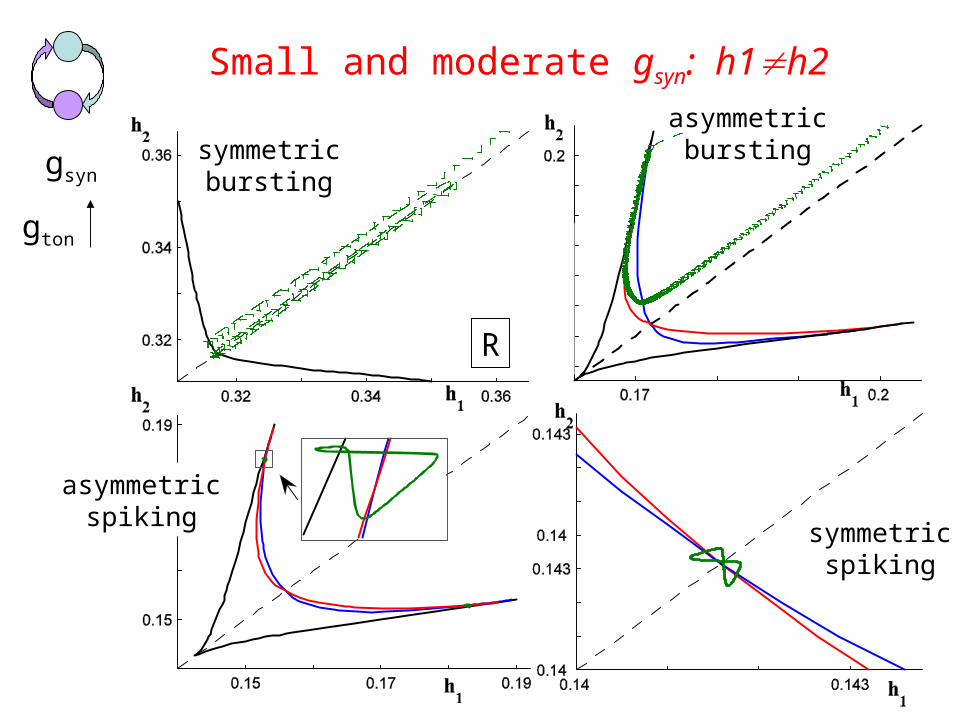
Small and moderate gsyn: h1h2

gsyn

gton

R

symmetricbursting

asymmetricbursting

asymmetricspiking

symmetricspiking

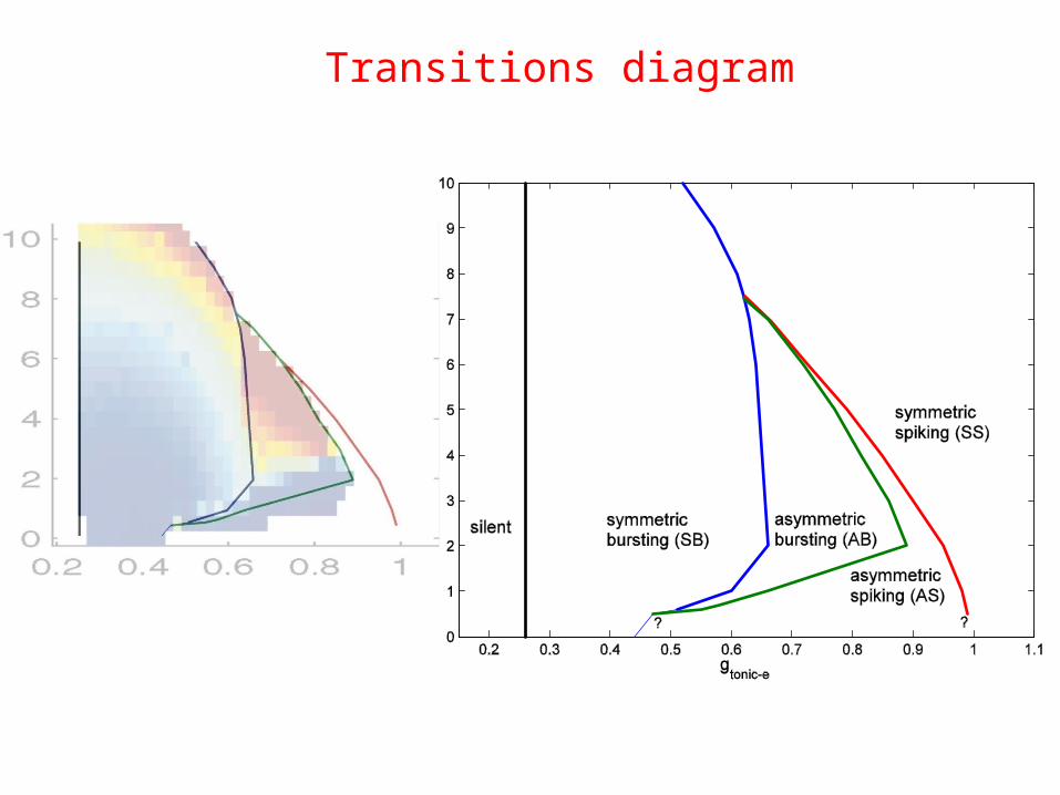
Transitions diagram

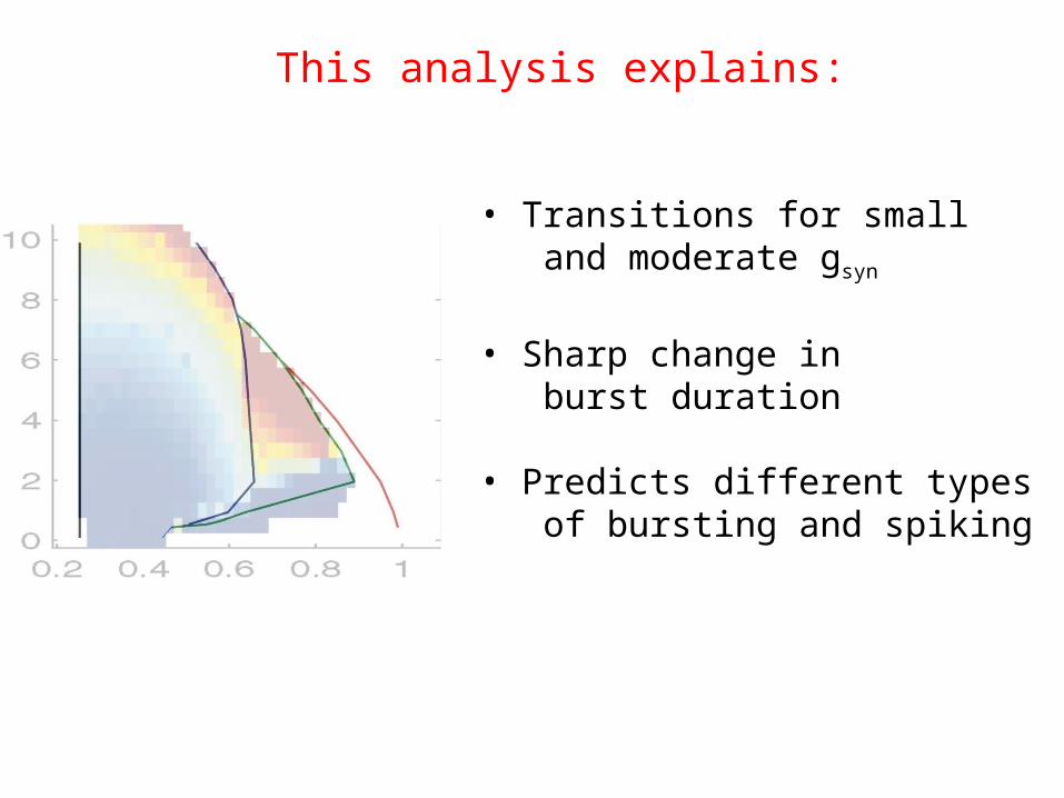
• Transitions for small and moderate gsyn

• Sharp change in burst duration

• Predicts different types of bursting and spiking

This analysis explains:

Conclusions

New in networks of bursting cells:

• Coupled square-wave bursters can generate top-hat bursting• Activity modes of coupled bursters can be characterized by considering phase space of averaged slow-variable equations

New predictions for experiments:

• Isolated cell has infrequent spikes at the end of a burst, but a cell in the network does not• In a pair of cells there can be two different types of bursting and two different types of spiking. Transitions can be made by changing gton

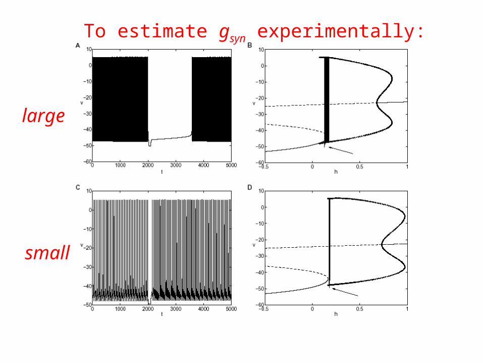
To estimate gsyn experimentally:

large

small

• J. Best, J. Rubin, D. Terman, M. Wechselberger• Supported by NSF (agreement No. 0112050) through Mathematical Biosciences Institute (MBI), OSU

Acknowledgments

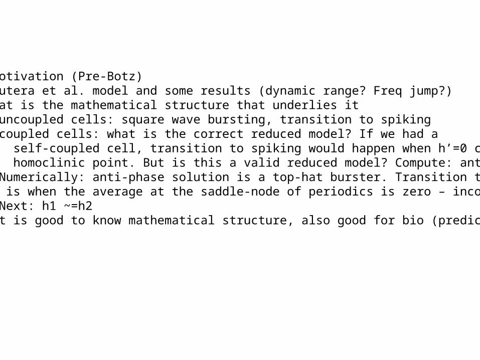
- Motivation (Pre-Botz)- Butera et al. model and some results (dynamic range? Freq jump?)-What is the mathematical structure that underlies it + uncoupled cells: square wave bursting, transition to spiking + coupled cells: what is the correct reduced model? If we had a self-coupled cell, transition to spiking would happen when h’=0 crosses homoclinic point. But is this a valid reduced model? Compute: anti-phase + Numerically: anti-phase solution is a top-hat burster. Transition to spiking is when the average at the saddle-node of periodics is zero – incorrect. + Next: h1 ~=h2 - It is good to know mathematical structure, also good for bio (predictions)

gton (type of cell)

g syn

(cou

plin

g st

reng

th)

gsyn

gton

gsyn

Range of bistability increases

gsyn

gton

Can transition to spiking

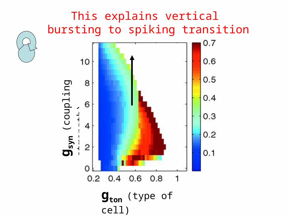
gton (type of cell)

g syn

(cou

plin

g st

reng

th)

This explains vertical bursting to spiking transition

2 experimental figuresDiff figure from butera et al for burst durationSlide for H functionsCorrect figure with h’sDifferent figure from JanetInsert schematic of h1-h2 plane