The Green Solow Model

William A. Brock*

M. Scott Taylor**

Abstract: We demonstrate that a key empirical �nding in environmental

economics - The Environmental Kuznets Curve - and the core model of modern

macroeconomics - the Solow model - are intimately related. Once we amend

the Solow model to incorporate technological progress in abatement, the EKC

is a necessary by product of convergence to a sustainable growth path. Our

amended model, which we dub the "Green Solow", generates an EKC relation-

ship between both the �ow of pollution emissions and income per capita, and

the stock of environmental quality and income per capita. The resulting EKC

may be humped shaped or strictly declining. We explain why current meth-

ods for estimating an EKC are likely to fail whenever they fail to account for

cross-country heterogeneity in either initial conditions or deep parameters. We

then develop an alternative empirical method closely related to tests of income

convergence employed in the macro literature. Preliminary tests of the model�s

predictions are investigated using data from OECD countries.

*Brock:Vilas Professor of Economics, Department of Economics, Univer-

sity of Wisconsin (wbrock@ssc.wisc.edu);**Taylor, Professor of Economics, De-

partment of Economics, University of Wisconsin, Faculty Research Associate

National Bureau of Economic Research, Cambridge, MA. (staylor@ssc.wisc.edu

and web: www.ssc.wisc.edu/~staylor). We thank Henning Bohn, Brian Copeland,

Steven Durlauf, John List, and conference participants at the UNCTEE 2004

conference at UC-Santa Barbara for helpful comments on an earlier draft. Ex-

cellent research assistance was provided by Pablo Pincheira. Research funding

was generously provided by the Vilas Trust, University of Wisconsin.

1

1 Introduction

The goal of this paper is to provide a cohesive theoretical explanation for three

puzzling features of the pollution and income per capita data. To do so we

introduce the reader to a very simple growth model closely related to the one-

sector Solow model. We show how this amended model generates predictions

closely in line with evidence on emissions, emission intensities and pollution

abatement costs. We then use this model to derive a simple estimating equation

linking a measure of emissions growth to initial emission levels and other controls

drawn from theory. Preliminary tests of the model are encouraging and well in

accord with the theoretical predictions of the Green Solow model.

Our work is related to recent attempts to explain the Environmental Kuznets

Curve (thereafter EKC) but di¤ers from other contributions in two important

ways. First, we attempt to �t more features of the data than just the EKC

and employ data on both pollution abatement costs and emission intensities

to identify key features of the data that are largely inconsistent with existing

theories. Second, we derive an estimating equation directly from our theory.

By doing so we provide the �rst rigorously developed link between theory and

empirical work in this area.

The EKC has captured the attention of policymakers, theorists and empirical

researchers alike since its discovery in the early 1990s. The theory literature

has from the start focussed on developing models that replicate the inverted U

shaped relationship. Prominent explanations are threshold e¤ects in abatement

that delay the onset of policy, income driven policy changes that get stronger

with income growth, structural change towards a service based economy, and

increasing returns to abatement that drive down costs of pollution control.1

While each of these explanations succeeds in predicting a EKC, they are

typically less successful at matching other features of the income and pollution

data. One key feature of this data concerns the timing of pollution reductions.

Models of threshold e¤ects predict no pollution policy at all over some initial

period followed by a period of active regulation.2 When policy is inactive,

emissions are produced lock step with output. When policy is active emissions

per unit of output fall as do aggregate emissions. As a result, the decline in the

1See for example Stokey (1998), Andreoni et al. (2001), and Lopez (1994) for originalcontributions. A review of the competing explanations appears in Chapter 2 of Copelandand Taylor (2003).

2This is for example the exact prediction of both Stokey (1998) and Brock and Taylor(2003a).

2

emissions to output ratio occurs simultaneously with the reduction in aggregate

pollution levels. This temporal correlation is however strongly contradicted by

the data.

1

1 0

1 0 0

1 9 5 0 1 9 5 5 1 9 6 0 1 9 6 5 1 9 7 0 1 9 7 5 1 9 8 0 1 9 8 5 1 9 9 0 1 9 9 5

Y e a r s

Tons

of E

mis

sion

s//D

olla

r

1940

=100

S ON O xV O C sP M 1 0C O

Figure 1: Emission Intensities

In Figure 1 we plot US data giving emissions per dollar of (real) GDP over the

1950 to 2001 period.3 For ease of reading we have adopted a log scale. We

plot emission intensities for sulfur dioxide, nitrogen dioxide, particulate matter,

carbon monoxide, and volatile organic compounds. There are two features of

note in the �gure. The �rst is simply that the emission to output ratio is in

decline from the start of the period in 1950. The second is that (given the

log scale for emissions per dollar of output) the percentage rate of decline has

been roughly constant over the �fty-year period (although it does vary across

pollutants).

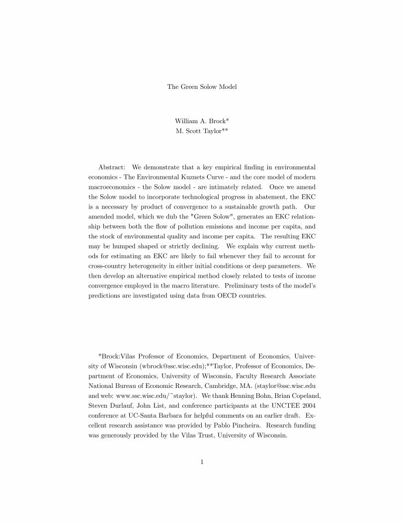
In Figure 2 we plot the corresponding emission levels for these same pol-

lutants over the same time period. Figure 2 shows a general tendency for3Data on US emissions of the criteria pollutants graphed in Figures 1 and 2

come from the US E.P.A. The long series of historical data presented in the �g-ures is taken from the EPA�s 1998 report National Pollution Emission Trends, athttp://www.epa.gov/ttn/chief/trends/trends.98. Because prior to 1985 fugitive dust sourcesand other miscellaneous emissions were not included in PM10 we have removed these compo-nents to make the data comparable over time.

3

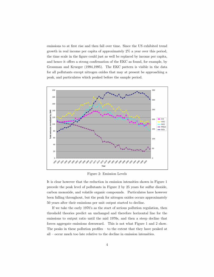
emissions to at �rst rise and then fall over time. Since the US exhibited trend

growth in real income per capita of approximately 2% a year over this period,

the time scale in the �gure could just as well be replaced by income per capita,

and hence it o¤ers a strong con�rmation of the EKC as found, for example, by

Grossman and Krueger (1994,1995). The EKC pattern is visible in the data

for all pollutants except nitrogen oxides that may at present be approaching a

peak, and particulates which peaked before the sample period.

0

20

40

60

80

100

120

140

160

180

200

1950

1952

1954

1956

1958

1960

1962

1964

1966

1968

1970

1972

1974

1976

1978

1980

1982

1984

1986

1988

1990

1992

1994

1996

1998

2000

Year

Tota

l em

issi

on n

orm

aliz

ed b

y 19

40

0

50

100

150

200

250

300

350

COVOCSO2PM10NOx

Figure 2: Emission Levels

It is clear however that the reduction in emission intensities shown in Figure 1

precede the peak level of pollutants in Figure 2 by 25 years for sulfur dioxide,

carbon monoxide, and volatile organic compounds. Particulates have however

been falling throughout, but the peak for nitrogen oxides occurs approximately

50 years after their emissions per unit output started to decline.

If we take the early 1970�s as the start of serious pollution regulation, then

threshold theories predict an unchanged and therefore horizontal line for the

emissions to output ratio until the mid 1970s, and then a steep decline that

forces aggregate emissions downward. This is not what Figure 1 and 2 show.

The peaks in these pollution pro�les � to the extent that they have peaked at

all � occur much too late relative to the decline in emission intensities.

4

A second feature of the data that is di¢cult to reconcile with many theo-

ries is the magnitude of pollution abatement costs. Theories that rely on rising

incomes driving down emissions via tighter pollution policy must square very

large reductions in emissions with very small pollution abatement costs. For

example in Figure 2, sulfur dioxide emissions peaked in 1973 at approximately

32,000 tons and fell almost in half to approximately 17,000 tons in 2001. Corre-

spondingly large changes in emissions per unit output also occurred. But over

much of this period, pollution abatement costs as a fraction of GDP or manufac-

turing value-added, remained both small and without much of a positive trend.

Theories that rely on tightening environmental policy predict ever increasing

costs of abatement, since emissions per unit of output must fall faster than ag-

gregate output to hold pollution in check. In a world without technological

progress in abatement, this requires larger and larger investments in pollution

control.4

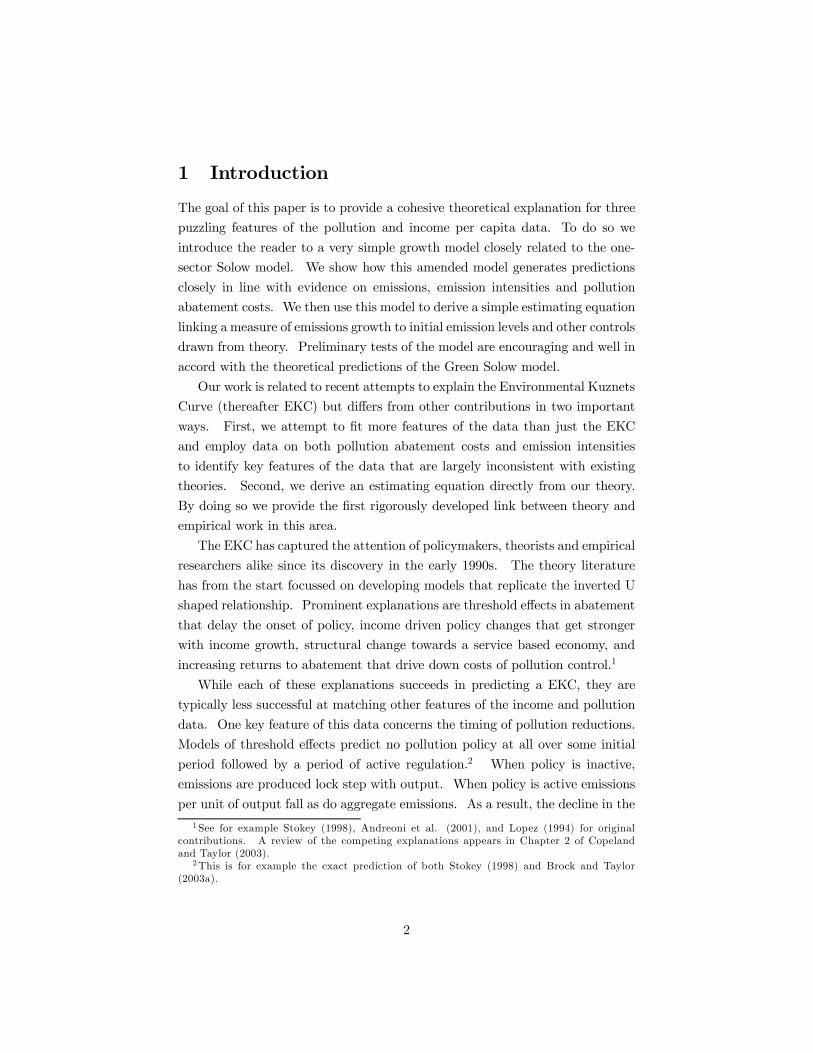
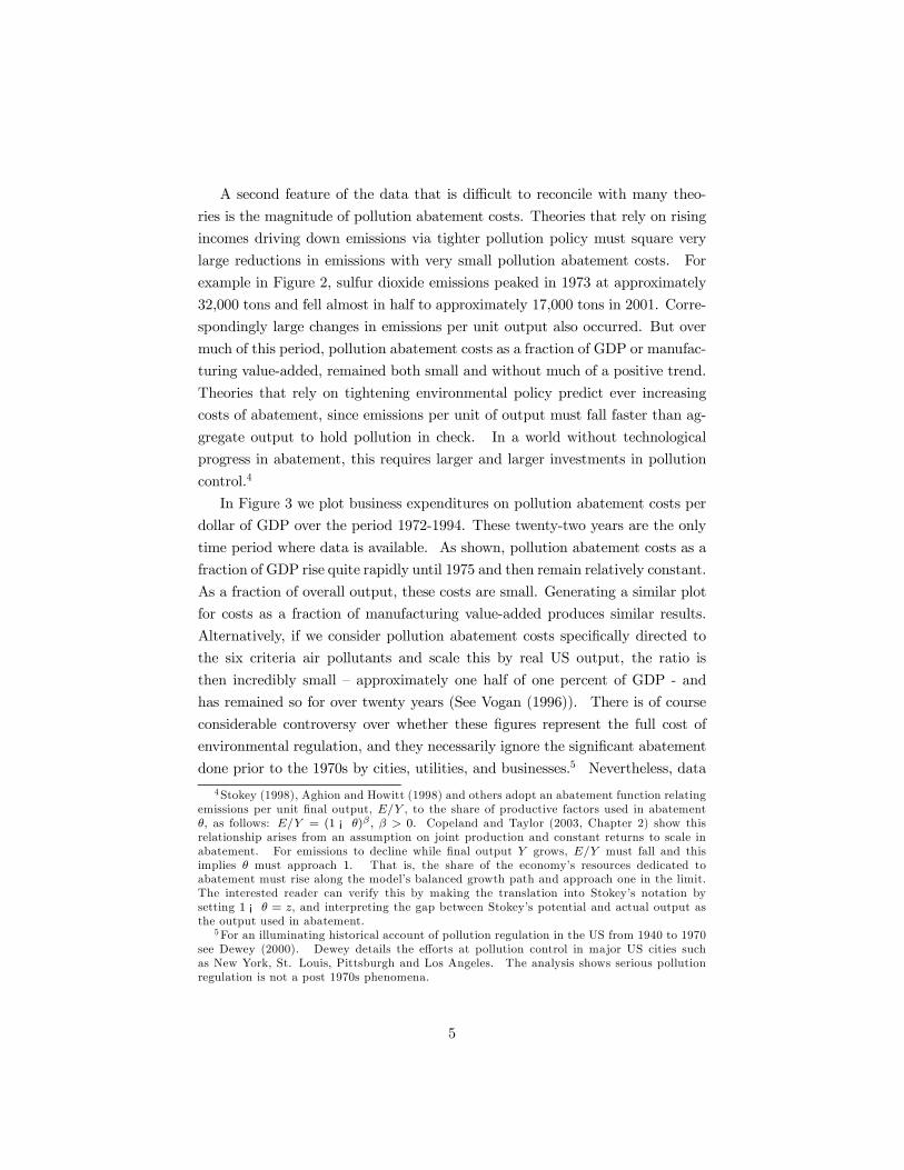
In Figure 3 we plot business expenditures on pollution abatement costs per

dollar of GDP over the period 1972-1994. These twenty-two years are the only

time period where data is available. As shown, pollution abatement costs as a

fraction of GDP rise quite rapidly until 1975 and then remain relatively constant.

As a fraction of overall output, these costs are small. Generating a similar plot

for costs as a fraction of manufacturing value-added produces similar results.

Alternatively, if we consider pollution abatement costs speci�cally directed to

the six criteria air pollutants and scale this by real US output, the ratio is

then incredibly small � approximately one half of one percent of GDP - and

has remained so for over twenty years (See Vogan (1996)). There is of course

considerable controversy over whether these �gures represent the full cost of

environmental regulation, and they necessarily ignore the signi�cant abatement

done prior to the 1970s by cities, utilities, and businesses.5 Nevertheless, data

4Stokey (1998), Aghion and Howitt (1998) and others adopt an abatement function relatingemissions per unit �nal output, !"# , to the share of productive factors used in abatement$, as follows: !"# = (1 ¡ $)! % & ' 0( Copeland and Taylor (2003, Chapter 2) show thisrelationship arises from an assumption on joint production and constant returns to scale inabatement. For emissions to decline while �nal output # grows, !"# must fall and thisimplies $ must approach 1. That is, the share of the economy�s resources dedicated toabatement must rise along the model�s balanced growth path and approach one in the limit.The interested reader can verify this by making the translation into Stokey�s notation bysetting 1 ¡ $ = ), and interpreting the gap between Stokey�s potential and actual output asthe output used in abatement.

5For an illuminating historical account of pollution regulation in the US from 1940 to 1970see Dewey (2000). Dewey details the e¤orts at pollution control in major US cities suchas New York, St. Louis, Pittsburgh and Los Angeles. The analysis shows serious pollutionregulation is not a post 1970s phenomena.

5

from other countries supports our general conclusion that pollution abatement

costs are a small fraction of GDP and show at best a slight upward trend.6

0.0%

0.2%

0.4%

0.6%

0.8%

1.0%

1.2%

1.4%

1.6%

1.8%

2.0%

1972 1973 1974 1975 1976 1977 1978 1979 1980 1981 1982 1983 1984 1985 1986 1987 1988 1989 1990 1991 1992 1993 1994

Year

Figure 3: US Abatement Costs/GDP

While income e¤ect theories often point to the creation of the EPA in the 1970s

and more activist environmental policy, we should again return to Figure 1 and

note that the trend in emissions to output was already declining and strongly so

prior to 1970. Therefore the advent of more activist federal policy in the 1970s

can only be a contributor to processes already at play in the 1950s.

Theories relying on strong compositional shifts or increasing returns also

have di¢culty matching these data. Changes in the composition of output

towards less pollution intensive goods can lower emissions in the medium term,

but in the long term reductions can only occur if emissions per unit of output

in the cleanest of goods falls. This of course places us back where we started,

asking how to lower emissions per unit output without ever rising costs. More-

over, empirical work has found a changing composition of output plays at most

a bit part in the reductions we have observed (Selden et al. (1997), Bruvoll et

al. (2003)).

And while increasing returns to abatement may be important in some in-

6US Data shown in Figure 3 is taken from Vogan (1996). See Table 3, section 4 forInternational data on pollution abatement costs, and our data appendix for a summary of themeasures used in our empirical work.

6

dustries and for some processes, a large portion of emissions come from small

di¤use sources such as cars, houses and individual consumptive activity. In

each of these cases, increasing returns to abatement seems unlikely. Increasing

returns also presents strong incentives for mergers and natural monopoly and

unless we bound the strength of increasing returns carefully, IRS models predict

negative pollution emissions at large levels of output.7

To us the pollution data and the related empirical work on the EKC present

three puzzles that need to be resolved by any successful theory.

The �rst puzzle is how do we square the very large reductions in emission

intensities shown in Figure 1 with the relatively small pollution abatement costs

shown in Figure 3?

The second puzzle is the EKC: what is responsible for the shape of the

pollution pro�les in Figure 2?

The third puzzle comes from the empirical literature itself. What explains

the current disconnect between the evidence for the EKC present in plots of raw

data like Figure 2, and the di¢culty empirical researchers have in estimating

EKC relationships? It is now well known that empirical estimates from EKC

style regressions can vary greatly with the sample used and estimation proce-

dure. How do we make sense of the �nding of an EKC in raw country level data

as shown in Figure 2, and the fragile cross-country empirical results that are

now commonplace to the literature?

In this paper we show that the Green Solow model provides a very simple

explanation for all three puzzles. Our explanation starts with the observations

in Figure 1 and 3. We square the rapidly declining emission intensities shown in

Figure 1 with the constant pollution abatement costs in Figure 3 by assuming

ongoing technological progress in abatement. To capture this possibility we

introduce exogenous technological progress into a standard abatement function

and then couple this abatement function with a standard �xed savings rate

Solow model. The resulting "Green Solow model" then generates a pattern of

incomes per capita and pollution consistent with Figure 2; i.e. it generates an

EKC.

The logic is simple: Ongoing technological progress in abatement drives

emissions per unit of output downward at a constant rate both in and out of

steady state (as in Figure 1). Initially the Solow model�s fast initial growth

7The simplest version of Andreoni and Levinson�s theory of increasing returns to abatementhas the property that pollution becomes negative for some large, but �nite level of output.This feature poses problems in dynamic models where output grows exponentially.

7

overwhelms progress in abatement to produce a period of initially rising emission

levels. Aggregate emissions rise even though emissions per unit of output

are falling (recall Figure 2). Technological progress in abatement however

eventually overwhelms the slowing growth of output as the economy approaches

its balanced growth path. Aggregate emissions start to decline while emissions

per unit of output continue their fall. Throughout the model�s measure of

pollution abatement costs as a fraction of GDP is constant (recall Figure 3).

We o¤er these features of the model as potential explanations for the �rst two

puzzles in the data.

Another model prediction is that the path for emissions, peak level of emis-

sions, and income per capita at peak emissions will typically be country speci�c.

Even countries that share identical parameter values will exhibit di¤erent EKC

patterns if they di¤er in initial conditions. Additional cross-country hetero-

geneity is introduced by di¤erences in savings rates, population growth rates

or abatement intensities. Failing to account for this heterogeneity could be

responsible for the failed empirical tests, and the sensitivity of estimates to the

sample. We take this feature of the model as a potential explanation for the

third puzzle - the current disconnect between the plots of raw data showing an

EKC within countries, and the fragility of cross country empirical results. While

much of current empirical work on the EKC includes controls for cross-country

heterogeneity these controls are typically level variables such as population den-

sity, openness to trade, or measures of democracy and not the rates of change

variables suggested by our analysis.

Finally to complete our argument, we provide empirical evidence in support

of our approach from sources outside the dataset we sought to explain. Since our

theoretical work shows that EKC pro�les are not unique we focus our attention

on a model prediction that holds more generally: convergence in a measure

of emissions per capita. By borrowing from techniques used in the macro

literature on income convergence we derive a simple linear estimating equation

linking growth in emissions per capita over a �xed time period to emissions

per capita in an initial period and a limited set of controls. These controls

include typical Solow type regressors such as population growth and the savings

rate, but also include a measure of pollution abatement costs and a proxy for

technological progress in abatement. To demonstrate the potential usefulness

of our approach we estimate our speci�cation on OECD data. The results are

encouraging.

Not surprisingly, the Green Solow model bears a family resemblance to many

8

other contributions in the literature given its close connection to Solow (1956).

It is similar in purpose to that of Stokey (1998) but di¤ers because Stokey

does not consider technological progress in abatement. It is related to the new

growth theory model of Bovenberg and Smulders (1995) because these authors

allow for "pollution augmenting technological progress", which is, under certain

circumstances, equivalent to our technological progress in abatement. The focus

of their work is however very di¤erent from ours. It is perhaps most closely

related to our own earlier work (Brock and Taylor (2003a)) where we tried to

match data on pollution abatement costs, the EKC, and emission intensities

within a modi�ed AK model with ongoing technological progress in both goods

and abatement production. While our earlier work was successful in some

respects, like other models with threshold e¤ects it failed to predict the steady

fall in emission to output ratios prior to peak pollution levels. And while this

earlier work contained a prediction regarding convergence in emission levels, this

prediction did not follow from the neoclassical forces we highlight here. This

paper grew out of our earlier attempts to match key features of the pollution

and income per capita data within the simplest model possible. Our work also

owes much to previous work in macroeconomics on conditional and absolute

convergence; in particular Barro (1991) and Barro and Sala-i-Martin (1992).

The rest of the paper proceeds as follows. Section 2 sets up the basic

model and develops three propositions concerning its behavior. In section 3

we derive an estimating equation from the model and present a preliminary

empirical implementation using CO2 data from the OECD. Section 4 contains

a discussion of our assumptions and o¤ers some international evidence. To

make our points clear we develop the model under the assumption that both

savings rates and abatement intensities are �xed over time. The appendix

contains all proofs and lengthy calculations.

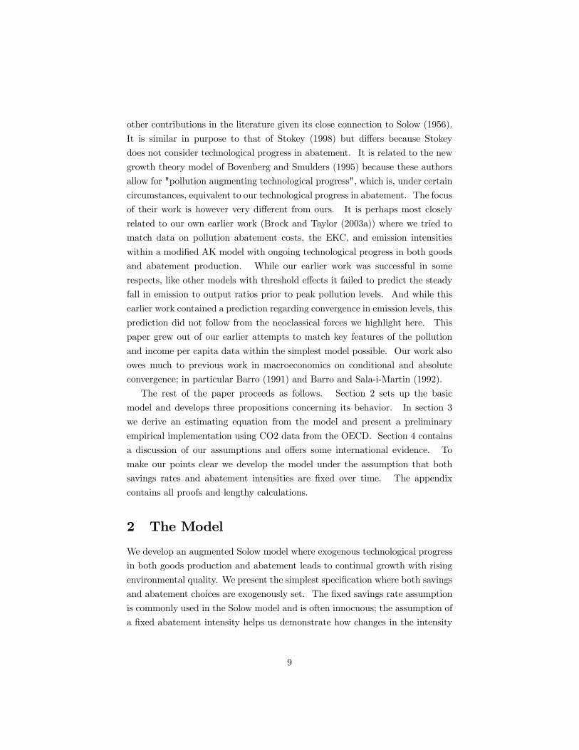
2 The Model

We develop an augmented Solow model where exogenous technological progress

in both goods production and abatement leads to continual growth with rising

environmental quality. We present the simplest speci�cation where both savings

and abatement choices are exogenously set. The �xed savings rate assumption

is commonly used in the Solow model and is often innocuous; the assumption of

a �xed abatement intensity helps us demonstrate how changes in the intensity

9

of abatement need not play any role in generating an Environmental Kuznets

Curve. Together they render the model simple and tractable.

Consider the standard one sector Solow model with a �xed savings rate

!. Output is produced via a constant returns to scale and strictly concave

production function taking e¤ective labor and capital to produce output, " .

Capital accumulates via savings and depreciates at rate #. We assume the rate

of labor augmenting technological progress is given by $. All this implies:

" = % (&'())'²& = !" ¡ #& (1)

²) = *)'

²( = $(

where ( represents labor augmenting technological progress and * is population

growth.

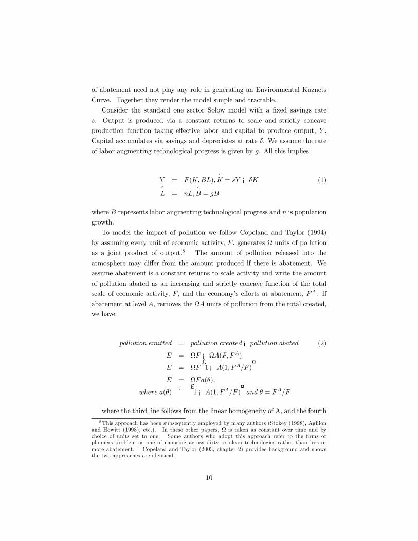
To model the impact of pollution we follow Copeland and Taylor (1994)

by assuming every unit of economic activity, % , generates ­ units of pollution

as a joint product of output.8 The amount of pollution released into the

atmosphere may di¤er from the amount produced if there is abatement. We

assume abatement is a constant returns to scale activity and write the amount

of pollution abated as an increasing and strictly concave function of the total

scale of economic activity, % , and the economy�s e¤orts at abatement, %!. If

abatement at level +, removes the ­+ units of pollution from the total created,

we have:

,-../01-* 2310024 = ,-../01-* 5627024¡ ,-../01-* 787024 (2)

9 = ­% ¡­+(%'%!)9 = ­%

£1¡+(1' %!:% )¤

9 = ­%7(;)'

<=262 7(;) ´ £1¡+(1' %!:% )¤ 7*4 ; = %!:%

where the third line follows from the linear homogeneity of A, and the fourth

8This approach has been subsequently employed by many authors (Stokey (1998), Aghionand Howitt (1998), etc.). In these other papers, ­ is taken as constant over time and bychoice of units set to one. Some authors who adopt this approach refer to the �rms orplanners problem as one of choosing across dirty or clean technologies rather than less ormore abatement. Copeland and Taylor (2003, chapter 2) provides background and showsthe two approaches are identical.

10

by the de�nition of ; as the fraction of economic activity dedicated to abate-

ment. We assume the intensive abatement function satis�es 7(0) = 1 and note

70(;) > 0 and 700(;) ? 0 by concavity. Abatement has a positive but diminish-ing marginal impact on pollution reduction. In some cases we will adopt the

speci�c form 7(;) = (1¡ ;)" where @ ? 1.The relationship in 2 requires several comments. The �rst is simply that 2

shows emissions are determined by the scale of economic activity % , and the

techniques of production as captured by ­7(;). Techniques can be in�uenced

by changes in the intensity of abatement, ;, or by technological progress that

lowers the parameter ­ over time. Since %! is included in % , even the activ-

ity of abatement itself pollutes. Second, abatement uses factors in the same

proportion as does �nal output hence we can think of the fraction ; of capital

and e¤ective labor being allocated directly to abatement with the remaining

fraction (1 ¡ ;) available for production of consumption or investment goods.

Finally, it is important to note that a �xed abatement intensity, ;' does not

correspond to a situation of static or non-existent environmental policy. We

show in the appendix that ; remains constant over time if governments raise

technology standards slowly over time. Our reading of environmental history

suggests this may be a reasonably accurate characterization of slowly evolving

technology standards imposed via command and control.

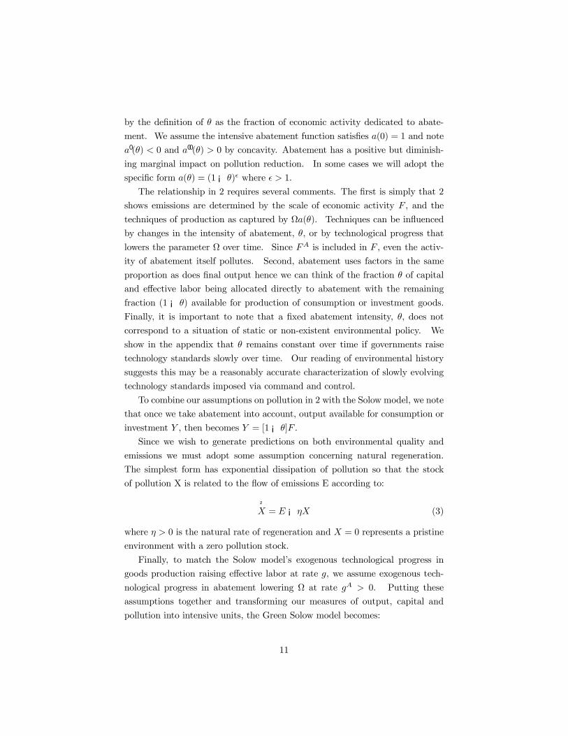
To combine our assumptions on pollution in 2 with the Solow model, we note

that once we take abatement into account, output available for consumption or

investment " , then becomes " = [1¡ ;]% .Since we wish to generate predictions on both environmental quality and

emissions we must adopt some assumption concerning natural regeneration.

The simplest form has exponential dissipation of pollution so that the stock

of pollution X is related to the �ow of emissions E according to:

²A = 9 ¡ BA (3)

where B ? 0 is the natural rate of regeneration and A = 0 represents a pristine

environment with a zero pollution stock.

Finally, to match the Solow model�s exogenous technological progress in

goods production raising e¤ective labor at rate $, we assume exogenous tech-

nological progress in abatement lowering ­ at rate $! ? 0. Putting these

assumptions together and transforming our measures of output, capital and

pollution into intensive units, the Green Solow model becomes:

11

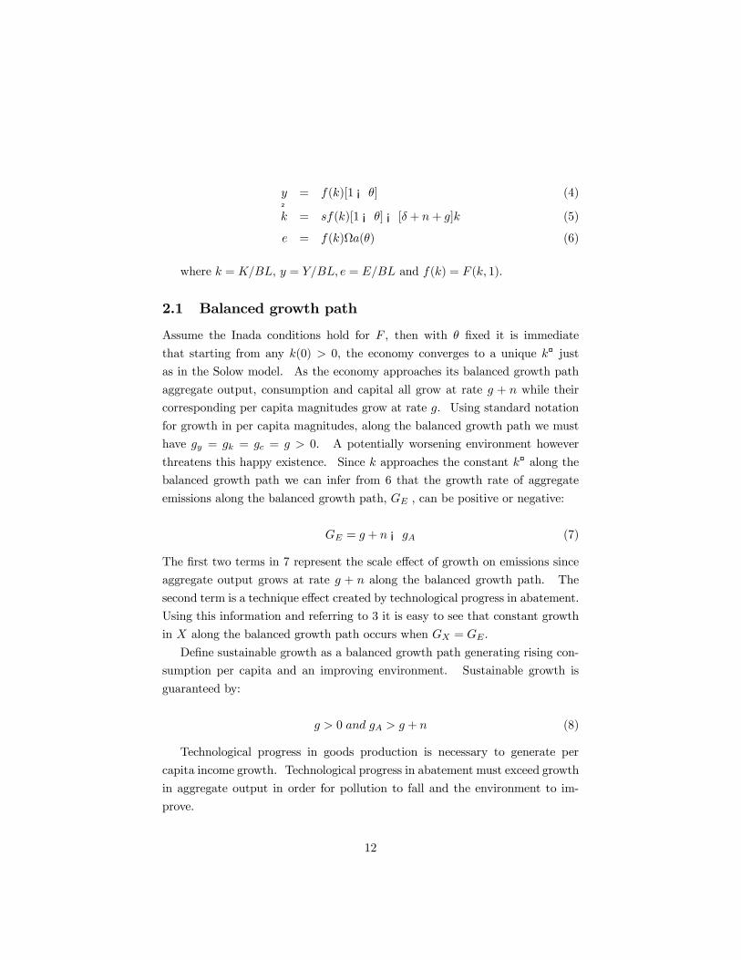
C = D(E)[1¡ ;] (4)²E = !D(E)[1¡ ;]¡ [# + *+ $]E (5)

2 = D(E)­7(;) (6)

where E = &:()' C = ":()' 2 = 9:() and D(E) = % (E' 1)F

2.1 Balanced growth path

Assume the Inada conditions hold for % , then with ; �xed it is immediate

that starting from any E(0) ? 0, the economy converges to a unique E¤ justas in the Solow model. As the economy approaches its balanced growth path

aggregate output, consumption and capital all grow at rate $ + * while their

corresponding per capita magnitudes grow at rate $. Using standard notation

for growth in per capita magnitudes, along the balanced growth path we must

have $# = $$ = $% = $ ? 0. A potentially worsening environment however

threatens this happy existence. Since E approaches the constant E¤ along thebalanced growth path we can infer from 6 that the growth rate of aggregate

emissions along the balanced growth path, G& , can be positive or negative:

G& = $ + *¡ $! (7)

The �rst two terms in 7 represent the scale e¤ect of growth on emissions since

aggregate output grows at rate $ + * along the balanced growth path. The

second term is a technique e¤ect created by technological progress in abatement.

Using this information and referring to 3 it is easy to see that constant growth

in A along the balanced growth path occurs when G' = G&.

De�ne sustainable growth as a balanced growth path generating rising con-

sumption per capita and an improving environment. Sustainable growth is

guaranteed by:

$ ? 0 7*4 $! ? $ + * (8)

Technological progress in goods production is necessary to generate per

capita income growth. Technological progress in abatement must exceed growth

in aggregate output in order for pollution to fall and the environment to im-

prove.

12

2.2 Green Solow and the EKC

The Green Solow model, although simple, generates a very suggestive explana-

tion for much of the empirical evidence relating income levels to environmental

quality. Despite the fact that the intensity of abatement is �xed, there are no

composition e¤ects in our one good framework, and no political economy or in-

tergenerational con�icts to resolve, the Green Solow model produces a path for

income per capita and environmental quality that traces out an Environmental

Kuznets Curve. This is true whether we measure environmental quality via our

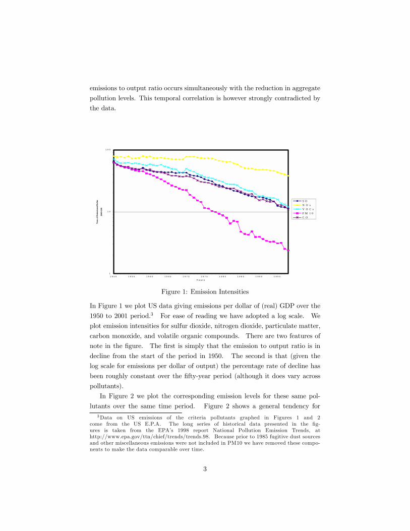
stock variable A or the �ow of emissions 9F This result is shown in Figure 4.9

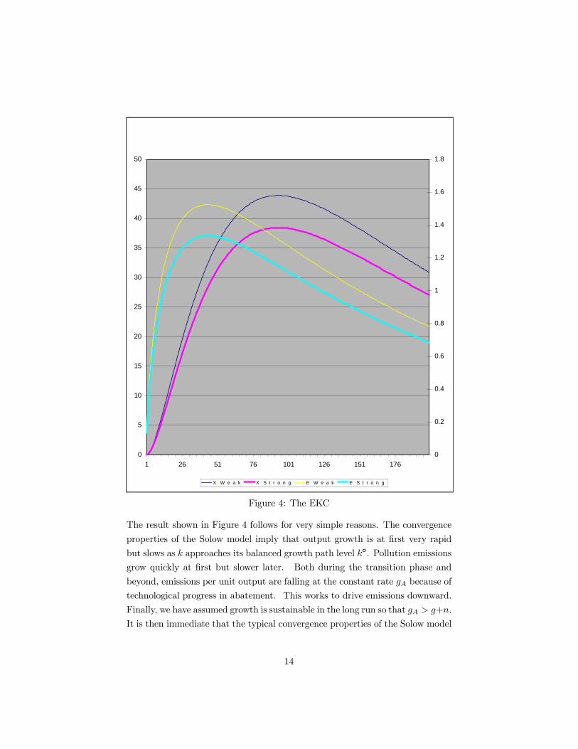
In Figure 4 we present the trajectories for two economies that are identical in

all respects except for their allocation to abatement ;. We plot both emissions

9 and the pollution stock A. Each economy starts from an initially pristine

environment and a small initial capital stock, E(0) ? 0. One economy allocates

5% of its output to abatement which we refer to as the strong abatement case;

the other economy is the weak abatement case as it allocates only .5% of its

output to abatement. Parameters were chosen for the purposes of illustration.

We have taken D(E) to be Cobb-Douglas with a capital share of .35. Per capita

income grows at 1.5% along the balanced growth path, the population grows at

1% and the abatement technology improves at 3%. These parameters ensure

sustainable growth is possible. The savings rate is 25%, depreciation is 3.5%,

regeneration is set at .03 implying a 3% rate of dissipation of X per unit time.

As shown, the environment at �rst worsens with both X and E rising. After

approximately 40 years emissions start to fall. After approximately 90 years

the pollution stock A, starts to fall and the economy converges on its balanced

growth path. Using 7 we know that along the balanced growth path emissions

fall at .5% per year, which is close to what the simulation delivers in its last

periods. Outside of the balanced growth path, emissions growth is of course

positive for a long period of time.

9During the �nal writing of this paper we discovered that Xepapadeas (2003) also notesthat technological progress in abatement can generate an EKC pattern. His discussion isbrief and appears in a review article as does our �rst discussion of Green Solow in Brock andTaylor (2003b).

13

0

5

10

15

20

25

30

35

40

45

50

1 26 51 76 101 126 151 1760

0.2

0.4

0.6

0.8

1

1.2

1.4

1.6

1.8

X W e a k X S t r o n g E W e a k E S t r o n g

Figure 4: The EKC

The result shown in Figure 4 follows for very simple reasons. The convergence

properties of the Solow model imply that output growth is at �rst very rapid

but slows as E approaches its balanced growth path level E¤. Pollution emissionsgrow quickly at �rst but slower later. Both during the transition phase and

beyond, emissions per unit output are falling at the constant rate $! because of

technological progress in abatement. This works to drive emissions downward.

Finally, we have assumed growth is sustainable in the long run so that $! ? $+*.

It is then immediate that the typical convergence properties of the Solow model

14

ensure that rapid growth in output will �rst overwhelm falling emissions per

unit output when the economy is far from its balanced growth path, but growth

in output will in turn be overwhelmed by technological progress in abatement

sometime before the economy enters its balanced growth path. The interplay

of technological progress and diminishing returns generates an EKC.

Outside observers may interpret the correlation between emission reduction

and income growth in a variety of ways. One interpretation could be that

environmental policy has �nally come of age and is now aggressive enough to

cause emission levels to fall. Another is that the slowdown in output growth

is caused by the tightening environmental policy that is also driving emissions

downward. Both of these interpretations are wrong in the context of the Green

Solow model. The decline in emissions is not re�ective of a new and invigorated

environmental policy since ; is constant over time. And the slowdown in

growth is caused by diminishing returns not environmental policy. In fact, the

slowdown in growth is the cause of emission decline - not the reverse. While

it is quite natural to link a turning point in emissions with a discrete change

in circumstances, the model shows that the turning point may instead re�ect a

more subtle weighing of various forces long at work in the economy.

In generating this result we have of course assumed the fraction of aggregate

resources allocated to abatement is roughly constant - recall Figure 3 - and we

have assumed technological progress in abatement works to lower emissions per

unit output continuously - recall Figure 1. In fact, Green Solow equates the

slope of log 9:" shown in Figure 1 to $! which we have assumed is constant

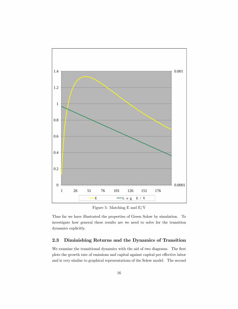
over time. Since the model predicts that emissions per unit of output fall

at a constant rate both during the transition period and along the balanced

growth path, emissions per unit of output are falling long before emissions or the

pollution stock peaks. It is tempting therefore to construct the model�s analog

to the emission intensities graphed in Figure 1 and pollution levels graphed in

Figure 2. We construct such a graph for the strong abatement case and present

it as Figure 5. The match with the earlier �gures is striking.

15

0

0.2

0.4

0.6

0.8

1

1.2

1.4

1 26 51 76 101 126 151 1760.0001

0.001

E L o g E / Y

Figure 5: Matching E and E/Y

Thus far we have illustrated the properties of Green Solow by simulation. To

investigate how general these results are we need to solve for the transition

dynamics explicitly.

2.3 Diminishing Returns and the Dynamics of Transition

We examine the transitional dynamics with the aid of two diagrams. The �rst

plots the growth rate of emissions and capital against capital per e¤ective labor

and is very similar to graphical representations of the Solow model. The second

16

follows from the �rst and plots the level of emissions as a function of capital per

e¤ective worker and is very similar to representations of the EKC. To start we

need to develop a di¤erential equation for emissions. To do so write emissions

at any time t as:

9 = ((0))(0)­(0)7(;) exp[G&0]E( (9)

where ((0), )(0), and ­(0) are initial conditions, and G& was given earlier.

Di¤erentiate with respect to time to obtain the growth rate of emissions:

²9

9= G& + H

²E

E(10)

where we note the rate of change of capital per e¤ective worker is simply:

²E

E= !E(¡1(1¡ ;)¡ (# + *+ $) (11)

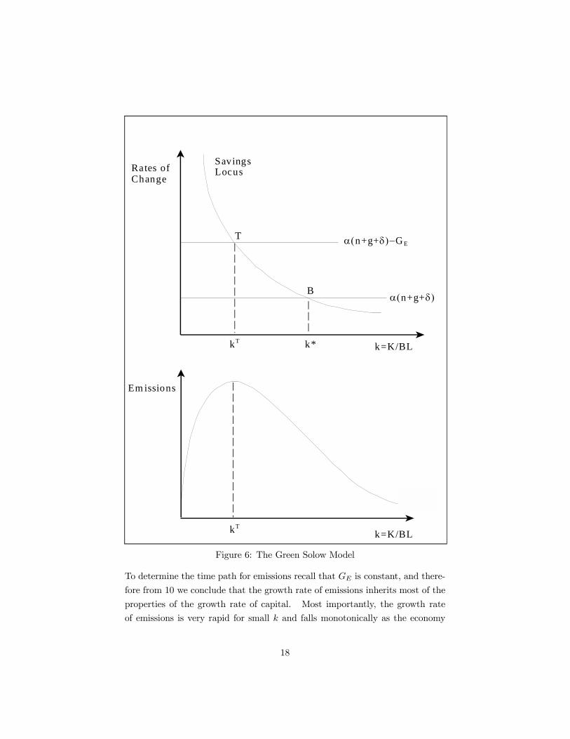
Using these two expressions we now depict the dynamics in the two panels of

Figure 6.

In the top panel of Figure 6 we plot the rates of change of (H times) capital

per e¤ective worker²HE:E and aggregate emissions

²9:9 on the vertical axis

against capital per e¤ective worker E on the horizontal. In drawing the �gure

we have implicitly assumed growth is sustainable. We refer to the negatively

sloped line as the savings locus since it is given by H!E(¡1[1¡;] and shifts withthe savings rate !F The savings locus starts at plus in�nity and approaches

zero as E grows large; therefore, it must intersect the two horizontal lines at

points T and B as shown. From 11 it is clear that the vertical distance between

H!E(¡1[1 ¡ ;] and the horizontal line with height H[# + *+ $] is just H times

the growth rate of capital per e¤ective worker or H²E:E. Capital per e¤ective

worker is rising at all points to the left of B and falling at all points to the

right. As is well known, the intersection at point B gives us the steady state

capital per e¤ective worker E¤. Growth is most rapid for small E and falls as

E approaches E¤F When the economy enters its balanced growth path,²E is zero

and the economy�s aggregate output and capital grow at rate $ + *.

17

k=K/BL

kT

T

B

!"n+g+#$%GE

!"n+g+#$

SavingsLocusRates of

Change

kT

Em issions

k*

k=K/BL

Figure 6: The Green Solow Model

To determine the time path for emissions recall that G& is constant, and there-

fore from 10 we conclude that the growth rate of emissions inherits most of the

properties of the growth rate of capital. Most importantly, the growth rate

of emissions is very rapid for small E and falls monotonically as the economy

18

approaches its balanced growth path. We will exploit this property later when

we derive an estimating equation predicting the convergence in emissions across

countries. But for now it is important to recognize that the growth rate of

emissions falls regardless of whether growth is sustainable or not.

To determine the peak level of emissions we use 10 and 11. By construction

the vertical distance between the savings locus H!E(¡1[1¡;] and the horizontalline with height H[# + * + $] ¡ G& equals the percentage rate of change of

emissions or²9:9F Therefore, at point T the growth rate of emissions is zero:

²9 = 0F Point T represents the turning point in emissions as shown in the bottom

panel of Figure 6. Under the assumption that growth is sustainable, G& > 0,

and point T lies to the left of B; when growth is not sustainable G& ? 0 and T

lies to the right of B.

The �gure illustrates several features of the model. It shows that if an

economy�s growth path is unsustainable, then emissions will grow ad in�nitum

even as the economy approaches its balanced growth path. But even in the

unsustainable case the growth rate of emissions falls along the transition path

until it approaches its balanced growth path rate from above. If growth is

sustainable then T lies to the left of B and the time pro�le for emission levels

depends on the location of E(0) relative to point T. If an economy starts with a

small initial capital stock then emissions at �rst rise and then fall as development

proceeds: i.e. we obtain an EKC pro�le for emissions. If initial capital is larger

it is possible that the level of emissions falls monotonically as the economy

moves towards its sustainable growth path. It is important to note while the

level of emissions may rise and then fall over time, the growth rate of emissions

is monotonically declining. This is apparent because emissions growth is rapid

for countries a long way from point B, and slower for those near B regardless

of the location of T. Finally when emissions peak depends on the relationship

between points T and B. For example, if ¡G& is small, then T and B di¤ervery little and emissions will only peak as the economy approaches its balanced

growth path which may of course take a very long time. Since these are key

results, we record them as a proposition.

Proposition 1 If growth is sustainable and E) ? E(0)' then the growth rate

of emissions is at �rst positive but turns negative in �nite time. If growth is

sustainable and E(0) ? E) ' then the growth rate of emissions is negative for

all t. If growth is unsustainable, then emissions growth declines with time but

remains positive for all t.

19

Proof: See Appendix

Proposition 1 tells us about the shape of the emissions and income pro�le but

says very little about the level of emissions and income per capita at the turning

point. Although the model is simple, it can be deceptive in this regard. For

example, it is a short step from knowing that E) is unique to an assumption that

income per capita at the turning point is unique. Similarly, it is easy to assume

that the path for income growth and emissions is the same for countries sharing

savings rates, population growth rates, etc. Both of these conjectures are wrong:

although E) is unique, the associated income per capita and emissions level at

E) are not.

Proposition 2 Economies with identical parameter values but di¤erent initialconditions produce di¤erent income per capita and emission pro�les over time.

The peak level of emissions and the level of income per capita associated with

peak emissions are not unique.

Proof: in text.

The intuition for this result is straightforward. The peak level of emissions is

reached when the rate of emissions growth created by output growth equals the

rate of technological progress in abatement. This occurs at a unique E) . Take

two economies with the same physical capital and assume both economies are

at E) . While these economies must have the same e¤ective labor force at this

point, one economy could have a highly e¢cient but small working population

while the other had a less e¢cient but more numerous labor force. Clearly

income per capita di¤er in these two economies even though each is at E) .

The nonuniqueness of emissions follows for related reasons. An economy

that is larger has greater emissions everywhere even though it may have the

same capital per e¤ective worker along the transition path as some hypothetical

smaller economy (see 9). Less transparently an economy with a inferior abate-

ment technology (a higher ­(0)) will have a higher emissions per unit of output

leading to a di¤erence in peak emissions at the turning point and elsewhere.

These examples highlight an important point brought out by the Green

Solow model. The current literature has tended to focus our attention on

level variables - speci�cally the level of pollution against the level of income per

capita. Even the "control variables" added to EKC regressions are often level

variables such as population density, openness to trade, measures of democracy

or deposits of coal. The Green Solow model refocuses our attention on growth

rates since it is the equality of two growth rates that determines the turning

20

point in emissions. By doing so it shows how looking at the levels of variables

can be misleading.

The non uniqueness of peak income and emission levels, o¤ers a potential

explanation for the contradictory and sometimes erratic empirical results found

in the EKC literature. It is now well known that the shape of the estimated

EKC can di¤er quite widely when researchers vary the time period of analysis,

the sample of countries, the pollutant, or even the data source. For example,

Harbaugh et al. (2002) reconsider Grossman and Krueger�s speci�cation and

�nd little support for an EKC using newer updated data. Stern and Common

(2001) employ a larger and di¤erent sulfur dioxide dataset and �nd no EKC.

And the literature reviews by both Barbier (1997) and Stern (2003) note that

published work di¤ers greatly in the estimated turning points for the EKC, the

standard errors on turning points are often very large, and empirical results di¤er

widely across pollutants and countries. At the same time, plots of raw pollution

data for the US and other countries often present a dramatic con�rmation of

the EKC.10

Proposition 2 o¤ers a simple explanation for the seeming inconsistency be-

tween country level data and cross-country empirical results. If EKC pro�les

for even very similar countries are not unique because of di¤erences in initial

conditions, then unobserved heterogeneity is surely a problem. Unobserved het-

erogeneity could then account for the large standard errors on turning points

and the sensitivity of results to the sample. While in theory conditioning on

country characteristics could eliminate the problem of unobserved heterogene-

ity, existing work has focussed on additional controls that are level variables

and not the rate of change variables suggested by our theory.

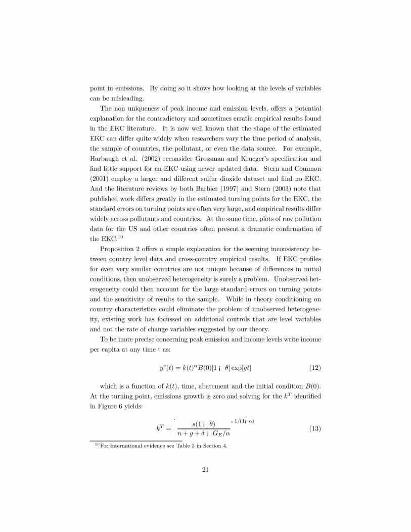
To be more precise concerning peak emission and income levels write income

per capita at any time t as:

C%(0) = E(0)(((0)[1¡ ;] exp[$0] (12)

which is a function of E(0)' time, abatement and the initial condition ((0)F

At the turning point, emissions growth is zero and solving for the E) identi�ed

in Figure 6 yields:

E) =

·!(1¡ ;)

*+ $ + # ¡G&:H¸1*(1¡()

(13)

10For international evidence see Table 3 in Section 4.

21

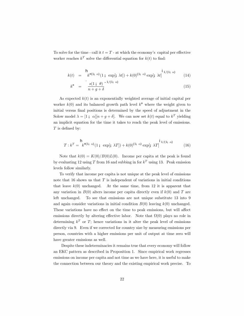
To solve for the time - call it 0 = I - at which the economy�s capital per e¤ective

worker reaches E) solve the di¤erential equation for E(0) to �nd:

E(0) =hE¤(1¡()(1¡ exp[¡J0]) + E(0)(1¡() exp[¡J0]

i1*(1¡()

(14)

E¤ =

·!(1¡ ;)*+ $ + #

¸1*(1¡()

(15)

As expected E(0) is an exponentially weighted average of initial capital per

worker E(0) and its balanced growth path level E¤ where the weight given toinitial versus �nal positions is determined by the speed of adjustment in the

Solow model J = [1¡ H][*+ $ + #]. We can now set E(0) equal to E) yieldingan implicit equation for the time it takes to reach the peak level of emissions.

I is de�ned by:

I : E) =hE¤(1¡()(1¡ exp[¡JI ]) + E(0)(1¡() exp[¡JI ]

i1*(1¡()

(16)

Note that E(0) = &(0):((0))(0). Income per capita at the peak is found

by evaluating 12 using I from 16 and subbing in for E) using 13. Peak emission

levels follow similarly.

To verify that income per capita is not unique at the peak level of emissions

note that 16 shows us that I is independent of variations in initial conditions

that leave E(0) unchanged. At the same time, from 12 it is apparent that

any variation in ((0) alters income per capita directly even if E(0) and I are

left unchanged. To see that emissions are not unique substitute 13 into 9

and again consider variations in initial condition ((0) leaving E(0) unchanged.

These variations have no e¤ect on the time to peak emissions, but will a¤ect

emissions directly by altering e¤ective labor. Note that ­(0) plays no role in

determining E) or I ; hence variations in it alter the peak level of emissions

directly via 9. Even if we corrected for country size by measuring emissions per

person, countries with a higher emissions per unit of output at time zero will

have greater emissions as well.

Despite these indeterminacies it remains true that every economy will follow

an EKC pattern as described in Proposition 1. Since empirical work regresses

emissions on income per capita and not time as we have here, it is useful to make

the connection between our theory and the existing empirical work precise. To

22

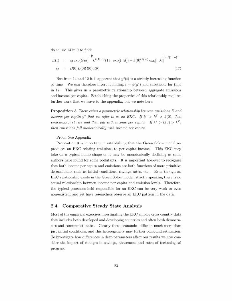
do so use 14 in 9 to �nd:

9(0) = 50 exp[G&0]

·hE¤(1¡()(1¡ exp[¡J0]) + E(0)(1¡() exp[¡J0]

i(*(1¡()¸

50 = ((0))(0)­(0)7(;) (17)

But from 14 and 12 it is apparent that C%(0) is a strictly increasing function

of time. We can therefore invert it �nding 0 = K(C%) and substitute for time

in 17. This gives us a parametric relationship between aggregate emissions

and income per capita. Establishing the properties of this relationship requires

further work that we leave to the appendix, but we note here:

Proposition 3 There exists a parametric relationship between emissions 9 andincome per capita C% that we refer to as an EKC. If E¤ ? E) ? E(0), then

emissions �rst rise and then fall with income per capita. If E¤ ? E(0) ? E) ,then emissions fall monotonically with income per capita.

Proof: See Appendix

Proposition 3 is important in establishing that the Green Solow model re-

produces an EKC relating emissions to per capita income. This EKC may

take on a typical hump shape or it may be monotonically declining as some

authors have found for some pollutants. It is important however to recognize

that both income per capita and emissions are both functions of more primitive

determinants such as initial conditions, savings rates, etc. Even though an

EKC relationship exists in the Green Solow model, strictly speaking there is no

causal relationship between income per capita and emission levels. Therefore,

the typical processes held responsible for an EKC can be very weak or even

non-existent and yet have researchers observe an EKC pattern in the data.

2.4 Comparative Steady State Analysis

Most of the empirical exercises investigating the EKC employ cross country data

that includes both developed and developing countries and often both democra-

cies and communist states. Clearly these economies di¤er in much more than

just initial conditions, and this heterogeneity may further confound estimation.

To investigate how di¤erences in deep parameters a¤ect our results we now con-

sider the impact of changes in savings, abatement and rates of technological

progress.

23

Consider the role of savings. An increase in the savings rate shifts the

savings locus rightward raising both T and B in Figure 6. Greater savings raises

capital per e¤ective worker in steady state. The turning point for emissions

rises because higher savings implies more rapid capital accumulation at each

E. This in turn means faster output growth and faster emissions growth at

any given EF The turning point can only be reached when diminishing returns

lowers output growth to meet ¡$!; greater savings makes this task harder andhence E) rises.

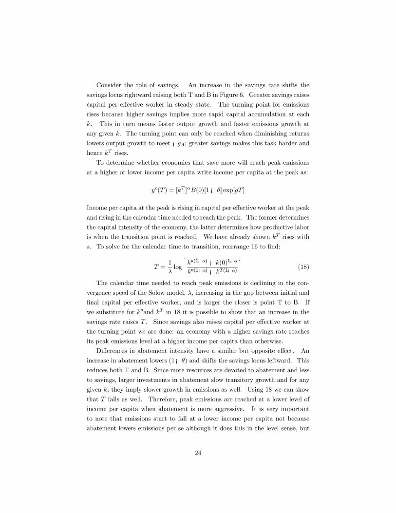
To determine whether economies that save more will reach peak emissions

at a higher or lower income per capita write income per capita at the peak as:

C%(I ) = [E) ](((0)[1¡ ;] exp[$I ]

Income per capita at the peak is rising in capital per e¤ective worker at the peak

and rising in the calendar time needed to reach the peak. The former determines

the capital intensity of the economy, the latter determines how productive labor

is when the transition point is reached. We have already shown E) rises with

!. To solve for the calendar time to transition, rearrange 16 to �nd:

I =1

Jlog

·E¤(1¡() ¡ E(0)1¡(

E¤(1¡() ¡ E) (1¡()

¸(18)

The calendar time needed to reach peak emissions is declining in the con-

vergence speed of the Solow model, J, increasing in the gap between initial and

�nal capital per e¤ective worker, and is larger the closer is point T to B. If

we substitute for E¤and E) in 18 it is possible to show that an increase in thesavings rate raises I . Since savings also raises capital per e¤ective worker at

the turning point we are done: an economy with a higher savings rate reaches

its peak emissions level at a higher income per capita than otherwise.

Di¤erences in abatement intensity have a similar but opposite e¤ect. An

increase in abatement lowers (1¡;) and shifts the savings locus leftward. Thisreduces both T and B. Since more resources are devoted to abatement and less

to savings, larger investments in abatement slow transitory growth and for any

given E, they imply slower growth in emissions as well. Using 18 we can show

that I falls as well. Therefore, peak emissions are reached at a lower level of

income per capita when abatement is more aggressive. It is very important

to note that emissions start to fall at a lower income per capita not because

abatement lowers emissions per se although it does this in the level sense, but

24

because abatement uses up scarce resources that would otherwise have gone to

investment. This reduces the rate of growth of output during the transition

period. It is the impact of abatement on growth rates during the transition that

alters E) . Changes in the abatement intensity have no e¤ect whatsoever on

the economy�s long run growth or on the long run growth rate of emissions.11

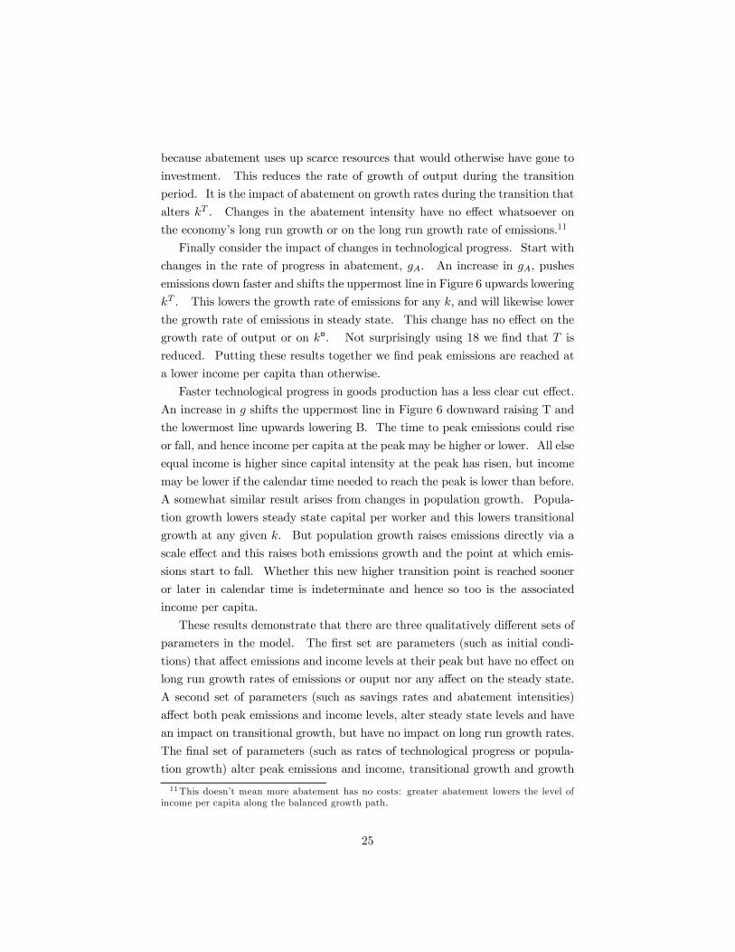
Finally consider the impact of changes in technological progress. Start with

changes in the rate of progress in abatement, $!. An increase in $!, pushes

emissions down faster and shifts the uppermost line in Figure 6 upwards lowering

E) . This lowers the growth rate of emissions for any E' and will likewise lower

the growth rate of emissions in steady state. This change has no e¤ect on the

growth rate of output or on E¤. Not surprisingly using 18 we �nd that I is

reduced. Putting these results together we �nd peak emissions are reached at

a lower income per capita than otherwise.

Faster technological progress in goods production has a less clear cut e¤ect.

An increase in $ shifts the uppermost line in Figure 6 downward raising T and

the lowermost line upwards lowering B. The time to peak emissions could rise

or fall, and hence income per capita at the peak may be higher or lower. All else

equal income is higher since capital intensity at the peak has risen, but income

may be lower if the calendar time needed to reach the peak is lower than before.

A somewhat similar result arises from changes in population growth. Popula-

tion growth lowers steady state capital per worker and this lowers transitional

growth at any given E. But population growth raises emissions directly via a

scale e¤ect and this raises both emissions growth and the point at which emis-

sions start to fall. Whether this new higher transition point is reached sooner

or later in calendar time is indeterminate and hence so too is the associated

income per capita.

These results demonstrate that there are three qualitatively di¤erent sets of

parameters in the model. The �rst set are parameters (such as initial condi-

tions) that a¤ect emissions and income levels at their peak but have no e¤ect on

long run growth rates of emissions or ouput nor any a¤ect on the steady state.

A second set of parameters (such as savings rates and abatement intensities)

a¤ect both peak emissions and income levels, alter steady state levels and have

an impact on transitional growth, but have no impact on long run growth rates.

The �nal set of parameters (such as rates of technological progress or popula-

tion growth) alter peak emissions and income, transitional growth and growth

11This doesn�t mean more abatement has no costs: greater abatement lowers the level ofincome per capita along the balanced growth path.

25

along a balanced growth path. In short these results demonstrate that the re-

lationship between income and pollution is exceedingly complex. And therefore

it should come as no surprise that there are large standard errors on turning

points and fragile coe¢cient estimates.

To our knowledge no empirical work examining the growth and environment

relationship has used as controls savings rates, population growth rates, etc.

that would be suggested by our analysis. But even with information on deep

parameters we have already shown that since the EKC pro�le is reliant on initial

conditions, estimation problems remain. One alternative that presents itself is

to focus on model predictions that are tightly linked to parameters: that is focus

on the relationship between the growth rate of emissions along the transition

path rather than the parametric relationship between the level of emissions and

income.

3 An Empirical Implementation

We have demonstrated why current empirical methods may have di¢culty in

estimating an EKC relationship. The income-emissions pro�le will di¤er across

countries if they di¤er in initial conditions or in basic parameters such as savings

or population growth rates. Criticism is of course much easier than creation,

and while many authors have been critical of the EKC methodology, very little

has been o¤ered as a productive alternative.

In this section we present an alternative method to investigate the growth

and environment relationship that draws on existing work in macroeconomics

on absolute and conditional convergence. Our goal is to develop an explicit link

between theory and empirical estimation since this link is largely absent in this

literature. A secondary goal is to demonstrate Green Solow�s ability to explain

cross-country patterns of emissions growth with relatively few variables.

The Green Solow model contains two empirical predictions regarding con-

vergence in emissions. The �rst is that a group of countries sharing the same

parameter values - savings rates, abatement intensities, rates of technological

progress etc. - but di¤ering in initial conditions will exhibit convergence in a

measure of their emissions. This is true even though each of these countries

would typically exhibit a unique income and pollution pro�le over time. We

will derive an estimating equation below to show that under the assumption of

identical parameters values across countries, we obtain a prediction of Absolute

26

Convergence in Emissions or ACE. Under the ACE hypothesis di¤erences in

the pattern of cross-country growth of emissions per person, is fully explained

by di¤erences in initial emissions per person. This prediction follows from the

familiar forces of diminishing returns plus an assumption that countries share

the same steady state.

The second prediction is that a disparate group of countries will exhibit both

very di¤erent pollution and income pro�les and will not exhibit ACE. Disparate

countries will grow outside of steady state at rates that are functions of both

di¤erences in initial conditions and di¤erences in country characteristics. In

theory if we condition on the right country characteristics, we could estimate a

relationship predicting convergence in emissions per person. Since this conver-

gence prediction is akin to the concept of conditional convergence in the macro

literature we refer to it as Conditional Convergence in Emissions. Here we

focus on the model�s predictions for ACE within a sample of OECD countries,

but also investigate how our results change when we allow countries to di¤er

in savings rates etc. We do so in order to generate and implement a testable

equation that may be of use to other researchers.

We conduct our empirical work with data on carbon dioxide emissions. We

focus on carbon dioxide for several reasons. Carbon dioxide data exists for

a large group of countries over a signi�cant period of time. The large cross

country coverage is important since it allows us to show that, as predicted,

ACE does not hold over the entire universe of countries in our sample. This

sample includes 139 developed and developing economies and this heterogeneity

should lead to the failure of ACE.

As well, researchers have had great di¢culty in making sense of the carbon

data. Estimates of the turning point for carbon are often very high and variable,

and hence carbon is one pollutant that may not follow an EKC. Given these

di¢culties, carbon o¤ers a good testing ground for our approach.

Finally very little direct abatement of carbon emissions has occurred. Some

reductions in carbon emissions have come about as a result of other pollution

regulations, but much of the trend in carbon emissions per unit output is related

to changes in the energy intensity of economies. But changes in energy use per

unit output and emissions per unit energy are thought to be responsible for a

majority of the reductions we have seen in the set of regulated pollutants.12

Therefore while carbon is unlike other pollutants because it is unregulated, it is

12 See for example Selden et al. (1999).

27

much like other air pollutants in that it is tightly tied to energy use.

3.1 Estimating Equation

We start with equation 9 for emissions but rewrite it in terms of emissions per

person 2%(0) = 9(0):)(0), and income per capita, C%(0) = % (0)[1 ¡ ;]:)(0).

Using standard notation, this gives us:

2%(0) = ­(0)~

7(;)C%(0) (19)

where~

7(;) = 7(;):[1¡ ;]. Di¤erentiating with respect to time yields

²2%

2%= ¡$! +

²C%

C%(20)

where we have made use of our assumption that the fraction of overall re-

sources dedicated to abatement is constant over time. As shown, growth in

emissions per person is the sum of technological progress in abatement plus

growth in income per capita. Along the balanced growth path this is equal

to ¡$! + $ which may be positive, negative, or zero; outside of the balancedgrowth path we will approximate the growth rate.

We make equation 20 operational in three steps. First approximate the

growth rate of income per capita and emissions per person over a discrete time

period of size N by their average log changes and rewrite the equation as:

[1:L ] log[2%+:2%+¡, ] = ¡$! + [1:L ] log[C%+:C%+¡, ] (21)

Second use the now standard procedures employed by Mankiw, Romer and

Weil (1992) and Barro (1991) to approximate the discrete N period growth rate

of income per capita near the model�s steady state via a log linearization to

obtain:13

[1:L ] log[C%+:C%+¡, ] = 8¡ [1¡ exp[¡JL ]

Llog[C%+¡, ] (22)

where 8 is a constant (discussed in more detail below) and J = [1¡H][*+$+#]is the Solow model�s speed of convergence towards E¤.Finally substitute for income growth in 21 using 22 and substitute for initial

13 See the appendix for a full derivation.

28

period income per capita using C%+¡, = 2+¡,:­!¡"

~

7(;) from equation 19.

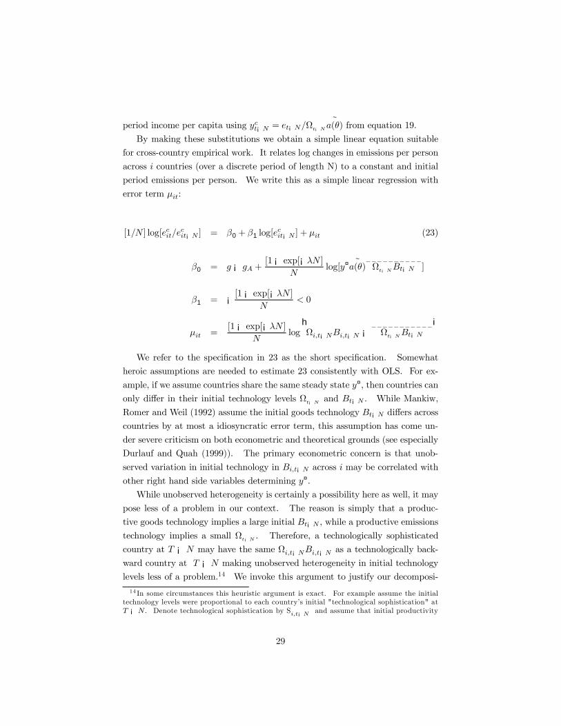
By making these substitutions we obtain a simple linear equation suitable

for cross-country empirical work. It relates log changes in emissions per person

across 1 countries (over a discrete period of length N) to a constant and initial

period emissions per person. We write this as a simple linear regression with

error term M-+:

[1:L ] log[2%-+:2%-+¡, ] = N0 + N1 log[2

%-+¡, ] + M-+ (23)

N0 = $ ¡ $! + [1¡ exp[¡JL ]L

log[C¤ ~

7(;)__________­!¡"(+¡, ]

N1 = ¡ [1¡ exp[¡JL ]L

> 0

M-+ =[1¡ exp[¡JL ]

Llog

h­-.+¡,(-.+¡, ¡

___________­!¡"(+¡,

iWe refer to the speci�cation in 23 as the short speci�cation. Somewhat

heroic assumptions are needed to estimate 23 consistently with OLS. For ex-

ample, if we assume countries share the same steady state C¤, then countries canonly di¤er in their initial technology levels ­!¡" and (+¡, . While Mankiw,

Romer and Weil (1992) assume the initial goods technology (+¡, di¤ers acrosscountries by at most a idiosyncratic error term, this assumption has come un-

der severe criticism on both econometric and theoretical grounds (see especially

Durlauf and Quah (1999)). The primary econometric concern is that unob-

served variation in initial technology in (-.+¡, across 1 may be correlated with

other right hand side variables determining C¤.While unobserved heterogeneity is certainly a possibility here as well, it may

pose less of a problem in our context. The reason is simply that a produc-

tive goods technology implies a large initial (+¡, , while a productive emissionstechnology implies a small ­!¡" . Therefore, a technologically sophisticated

country at I ¡L may have the same ­-.+¡,(-.+¡, as a technologically back-

ward country at I ¡L making unobserved heterogeneity in initial technology

levels less of a problem.14 We invoke this argument to justify our decomposi-

14 In some circumstances this heuristic argument is exact. For example assume the initialtechnology levels were proportional to each country�s initial "technological sophistication" at* ¡+ . Denote technological sophistication by S"#$¡% and assume that initial productivity

29

tion of the unobservable country speci�c products ­-.!¡"(-.+¡, into an overall

cross country mean we denote by__________­!¡"(+¡, plus a country speci�c devia-

tion. These country speci�c deviations plus standard approximation error in

generating our linear form are contained in our error term M-+ as shown above.

OLS is consistent if the covariance of M-+ and our right hand side variables is

zero.

Since individual elements making up the constant term in 23 are not iden-

ti�ed we have no prediction concerning the sign. The growth rate of emissions

per person should however fall with higher initial period emissions per person

and this is re�ected in the prediction of N1 > 0 The intuition for this is simple.

Holding the technology levels and abatement intensity �xed, a lower emissions

per person 2%+¡, corresponds to a lower initial capital per e¤ective worker E+¡, .This then implies a rapid rate of growth in aggregate emissions 9 and hence

a rapid rate of growth of emissions per person. It is also useful to note that

since L is given, any estimate of N1 carries with it an implicit estimate of the

rate of convergence of the Solow model, J. Since L is �xed, we can back out

these estimates of J and check them against those provided by the cross-country

growth literature.

While the short speci�cation is simple it is also unsatisfactory. It is unsat-

isfactory because the Green Solow�s key predictions on emissions follow from

the new element $! and the reliance of C¤ and 7(;) on abatement. Thus far

we have assumed $! and ; are both constant over time and exhibit no cross

country variation. But data on these variables are available. Cross country

data on the share of pollution abatement costs in GDP shows ; varies little over

time, but exhibits substantial cross country variation. Moreover if we take our

model literally then $! equals the rate at which carbon emissions to output falls

over time. This ratio is both observable and does vary across countries.

To carry forward these new elements into empirical work we now construct

the long speci�cation of our estimating equation. To do so it proves useful to

assume 7(;) = (1¡ ;)" where @ ? 1F This formulation follows from a constant

returns abatement function, and like all isoelastic functions it is quite useful

in empirical work. To generate our long speci�cation we return to our short

speci�cation in 23. Let savings, abatement, $!, and the e¤ective depreciation

rate (* + $ + #) vary across countries by taking on an 1 subscript, and then

is proportional to technological sophistication; that is, ­"#$¡% = ,"-"#$¡% and ."#$¡% =/-"#$¡% for some , and / positive. Note the product ­"#$¡%."#$¡% = ,/ which is nowindependent of 0.

30

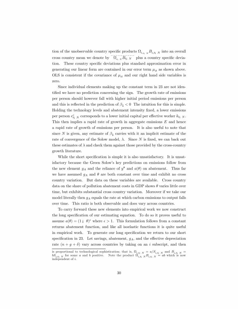
substitute for the determinants of C¤ to write the long speci�cation as:

[1:L ] log[2%-+:2%-+¡, ] = N0 + N1 log[2

%-+¡, ] + N2[$!-] (24)

+N3 log[!-] + N4 log[1¡ ;]-

+N5 log[(*+ $ + #)]- + M-+

N0 = $ +[1¡ exp[¡JL ]

L[log

___________­!¡"(+¡, ]

N1 = ¡ [1¡ exp[¡JL ]]L

> 0'

N2 = ¡1 > 0

N3 = [H:(1¡ H)] [1¡ exp[¡JL ]L

? 0

N4 = [H:(1¡ H) + @¡ 1] [1¡ exp[¡JL ]L

? 0

N5 = ¡N3 > 0

where $!- is a country speci�c estimate of technological progress in abate-

ment (see below), while !-, [1 ¡ ;]- and [(* + $ + #)]- are the time-averaged

country speci�c savings rate, abatement, and e¤ective depreciation rate respec-

tively. Savings and depreciation are familiar from growth regressions as are

several of the restrictions theory imposes on coe¢cient magnitudes. The long

speci�cation does however add new parameters to estimate and provides two

new testable restrictions.

Given our earlier discussions it should be apparent that an increase in sav-

ings raises the growth rate of emissions per person by raising the steady state

capital stock. This positive transitional e¤ect of savings on emissions growth

is captured by N3 ? 0. Since a reduction in abatement raises the economy�s

steady state capital intensity and raises emissions via reduced abatement, we

31

also have N4 ? 0. The coe¢cient sign of N5 follows directly from the role

"e¤ective depreciation" plays in determining a country�s steady state capital

intensity.

Apart from the usual parameter restrictions contained in the Solow model

(N5 + N3 = 0' and H should be close to capital�s share) the Green Solow model

contains the additional restriction of a unitary coe¢cient on $! and N4 ¡N3 ? 0F

Moreover, by judicious use of estimates for N1' N3 and N4 an estimate for @ can

be constructed. Again, since L is known, we can recover an estimate of J as

well.

There are however new econometric and data complications introduced by

the long speci�cation. One concern is a common one. We do not have data

for either $ or #, and hence we have to construct our regressor (*+ $+ #) using

alternative means. Here we follow the literature in assuming $ + # = F05, and

then use observed population growth rates for * to construct the regressor. A

second complication arises because strictly speaking once we admit population

di¤erences across countries, we should also admit di¤erences across countries in

the parameter J as well. Since doing so would exhaust our degrees of freedom

we again follow the literature in treating J as constant across countries. Since

this is somewhat unsatisfactory we will investigate how the inclusion of e¤ective

depreciation a¤ects our results.

Finally since technological progress in abatement is a key part of our theory

we construct a measure of $-.!. This is somewhat problematic since our theory

takes $-.! to be exogenous and hence is uninformative on its determinants.15

But since we are taking the intensity of abatement as �xed over time, we could

in theory obtain estimates for $-.! by regressing ln(9-+:"-+) on a constant and

a time trend. This speci�cation follows directly from our theory�s prediction

for E/Y as given for example in 9. It seems likely however that although

technological progress may be the largest force a¤ecting the time pro�le for

15One generalization that may be worth pursuing is to assume that �nal output is producedby a continuum of inputs each with a di¤erent pollution intensity. In this case we can then

write an economy�s overall emission intensity as: !"# =

!­()% 1),()% $)&(')((')

)2) where the

integral is de�ned over the set of available inputs; ­()% 1),()% $) is emission per dollar of �naloutput in sector ), and 3())4()) is total dollar value added in this sector. Let industry shares

be given by /()% 1) = 3())4())"# , with!/()% 1)2) = 1. Then straightforward di¤erentiation

will show that even if the rate of technological progress in abatement is identical across sectors(i.e. assume ­()% 1) is independent of z), then the rate of change in !"# will di¤er from 5*if there are compositional changes in the economy. This suggests that our crude method forestimating 5* could be improved by employing information on sectoral shares and carbonintensity. We intend to investigate this possibility in the future.

32

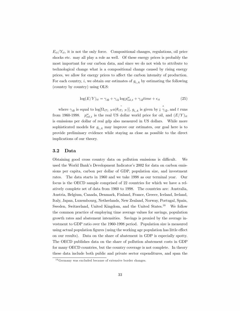
9-+:"-+, it is not the only force. Compositional changes, regulations, oil price

shocks etc. may all play a role as well. Of these energy prices is probably the

most important for our carbon data, and since we do not wish to attribute to

technological change what is a compositional change caused by rising energy

prices, we allow for energy prices to a¤ect the carbon intensity of production.

For each country, 1, we obtain our estimates of $-.! by estimating the following

(country by country) using OLS:

log(9:" )-+ = O-0 + O-1 log ,/0-1.+ + O-20132+ @-+ (25)

where O-0 is equal to log[­-)¡,~

7(;-)¡,)], $-.! is given by^¡O-2, and 0 runs

from 1960-1998. ,/0-1.+ is the real US dollar world price for oil, and (9:" )-+is emissions per dollar of real gdp also measured in US dollars. While more

sophisticated models for $-.! may improve our estimates, our goal here is to

provide preliminary evidence while staying as close as possible to the direct

implications of our theory.

3.2 Data

Obtaining good cross country data on pollution emissions is di¢cult. We

used the World Bank�s Development Indicator�s 2002 for data on carbon emis-

sions per capita, carbon per dollar of GDP, population size, and investment

rates. The data starts in 1960 and we take 1998 as our terminal year. Our

focus is the OECD sample comprised of 22 countries for which we have a rel-

atively complete set of data from 1960 to 1998. The countries are: Australia,

Austria, Belgium, Canada, Denmark, Finland, France, Greece, Iceland, Ireland,

Italy, Japan, Luxembourg, Netherlands, New Zealand, Norway, Portugal, Spain,

Sweden, Switzerland, United Kingdom, and the United States.16 We follow

the common practice of employing time average values for savings, population

growth rates and abatement intensities. Savings is proxied by the average in-

vestment to GDP ratio over the 1960-1998 period. Population size is measured

using actual population �gures (using the working age population has little e¤ect

on our results). Data on the share of abatement in GDP is especially spotty.

The OECD publishes data on the share of pollution abatement costs in GDP

for many OECD countries, but the country coverage is not complete. In theory

these data include both public and private sector expenditures, and span the

16Germany was excluded because of extensive border changes.

33

years 1985 to 1998, but few countries have complete coverage.17 Accordingly we

employ averages over the longest period possible and employ the widest measure

for pollution abatement cost available (public plus private expenditures when

available). For some countries the time averaged estimates re�ects relatively

few observations. In order not to lose degrees of freedom we calculated the

share for Luxembourg directly from OECD sources, and assumed New Zealand

had the same abatement intensity as its neighbor Australia. Given the quality

of this data the reader is cautioned from drawing strong conclusions from our

results.

3.3 Results

We start by examining the possibility of absolute convergence in emissions. It

would of course be surprising to �nd ACE supported across anything but the

most homogenous of country groupings. We expect ACE to fail miserably

because any broad set of countries will di¤er greatly in their rates of savings,

population growth and technological progress.

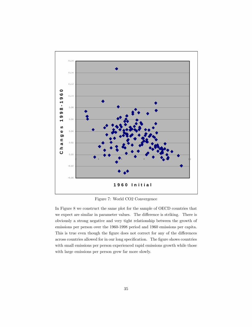
As a starting point for our analysis we present in Figure 7 the yearly average

log changes in emissions per person against the log of initial levels for 139

countries available in the World Bank development indicators.18 As the plot

shows there is little apparent relationship between the two series.

17This data is available from the OECD publication "Pollution abatement and controlexpenditures in OECD Countries", Paris: OECD Secretariat. We present our pollutionabatement cost data in the appendix.18This plot includes all countries in the database for which there is data in 1960. Emissions

are measured in lbs of emissions per capita for ease of reading.

34

-0.04

-0.02

0.00

0.02

0.04

0.06

0.08

0.1 0

0.1 2

0.1 4

0.1 6

2 4 6 8 10 12

1 9 6 0 I n i t i a l

C h

a n

g e

s

1 9

9 8

- 1 9

6 0

Figure 7: World CO2 Convergence

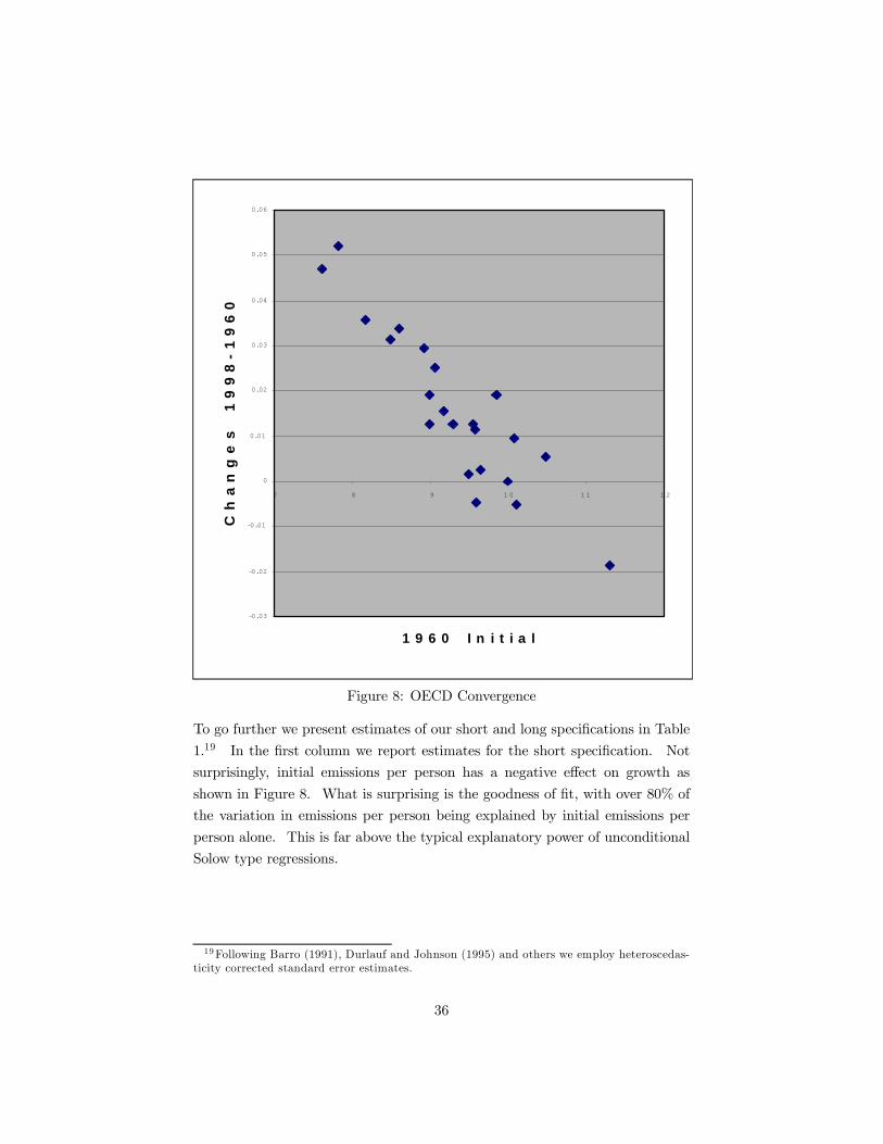
In Figure 8 we construct the same plot for the sample of OECD countries that

we expect are similar in parameter values. The di¤erence is striking. There is

obviously a strong negative and very tight relationship between the growth of

emissions per person over the 1960-1998 period and 1960 emissions per capita.

This is true even though the �gure does not correct for any of the di¤erences

across countries allowed for in our long speci�cation. The �gure shows countries

with small emissions per person experienced rapid emissions growth while those

with large emissions per person grew far more slowly.

35

-0.03

-0.02

-0.01

0

0.01

0.02

0.03

0.04

0.05

0.06

7 8 9 1 0 1 1 1 2

1 9 6 0 I n i t i a l

C h

a n

g e

s

1 9

9 8

- 1

9 6

0

Figure 8: OECD Convergence

To go further we present estimates of our short and long speci�cations in Table

1.19 In the �rst column we report estimates for the short speci�cation. Not

surprisingly, initial emissions per person has a negative e¤ect on growth as

shown in Figure 8. What is surprising is the goodness of �t, with over 80% of

the variation in emissions per person being explained by initial emissions per

person alone. This is far above the typical explanatory power of unconditional

Solow type regressions.

19Following Barro (1991), Durlauf and Johnson (1995) and others we employ heteroscedas-ticity corrected standard error estimates.

36

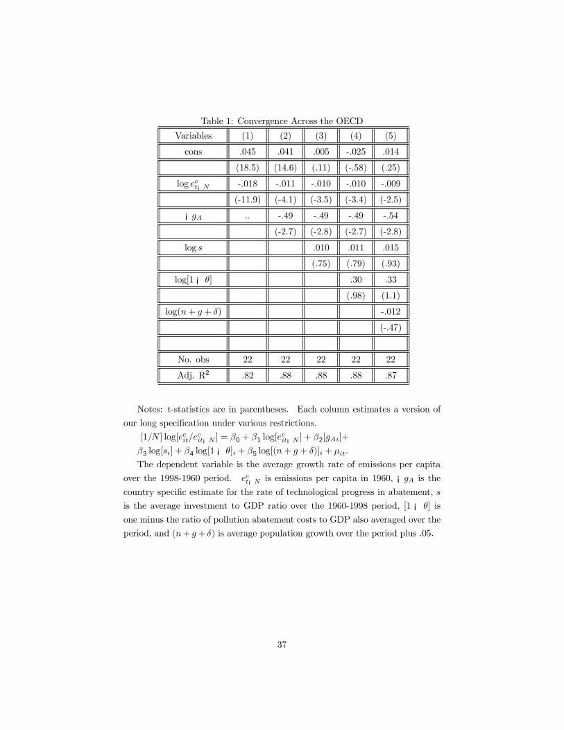
Table 1: Convergence Across the OECD

Variables (1) (2) (3) (4) (5)

cons .045 .041 .005 -.025 .014

(18.5) (14.6) (.11) (-.58) (.25)

log 2%+¡, -.018 -.011 -.010 -.010 -.009

(-11.9) (-4.1) (-3.5) (-3.4) (-2.5)

¡$! .. -.49 -.49 -.49 -.54

(-2.7) (-2.8) (-2.7) (-2.8)

log ! .010 .011 .015

(.75) (.79) (.93)

log[1¡ ;] .30 .33

(.98) (1.1)

log(*+ $ + #) -.012

(-.47)

No. obs 22 22 22 22 22

Adj. R2 .82 .88 .88 .88 .87

Notes: t-statistics are in parentheses. Each column estimates a version of

our long speci�cation under various restrictions.

[1:L ] log[2%-+:2%-+¡, ] = N0 + N1 log[2

%-+¡, ] + N2[$!-]+

N3 log[!-] + N4 log[1¡ ;]- + N5 log[(*+ $ + #)]- + M-+.

The dependent variable is the average growth rate of emissions per capita

over the 1998-1960 period. 2%+¡, is emissions per capita in 1960, ¡$! is thecountry speci�c estimate for the rate of technological progress in abatement, !

is the average investment to GDP ratio over the 1960-1998 period, [1 ¡ ;] is

one minus the ratio of pollution abatement costs to GDP also averaged over the

period, and (*+ $+ #) is average population growth over the period plus .05.

37

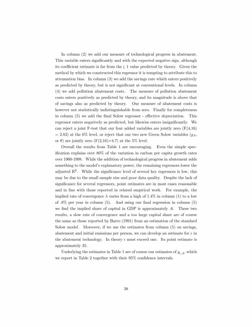
In column (2) we add our measure of technological progress in abatement.

This variable enters signi�cantly and with the expected negative sign, although

its coe¢cient estimate is far from the ¡1 value predicted by theory. Given themethod by which we constructed this regressor it is tempting to attribute this to

attenuation bias. In column (3) we add the savings rate which enters positively

as predicted by theory, but is not signi�cant at conventional levels. In column

(4) we add pollution abatement costs. The measure of pollution abatement

costs enters positively as predicted by theory, and its magnitude is above that

of savings also as predicted by theory. Our measure of abatement costs is

however not statistically indistinguishable from zero. Finally for completeness

in column (5) we add the �nal Solow regressor - e¤ective depreciation. This

regressor enters negatively as predicted, but likewise enters insigni�cantly. We

can reject a joint F-test that our four added variables are jointly zero (F(4,16)

= 2.82) at the 6% level, or reject that our two new Green Solow variables ($!,

or ;) are jointly zero (F(2,16)=4.7) at the 5% level.

Overall the results from Table 1 are encouraging. Even the simple spec-

i�cation explains over 80% of the variation in carbon per capita growth rates

over 1960-1998. While the addition of technological progress in abatement adds

something to the model�s explanatory power, the remaining regressors lower the

adjusted R2. While the signi�cance level of several key regressors is low, this

may be due to the small sample size and poor data quality. Despite the lack of

signi�cance for several regressors, point estimates are in most cases reasonable

and in line with those reported in related empirical work. For example, the

implied rate of convergence J varies from a high of 1.4% in column (1) to a low

of .8% per year in column (5). And using our �nal regression in column (5)

we �nd the implied share of capital in GDP is approximately .6. These two

results, a slow rate of convergence and a too large capital share are of course

the same as those reported by Barro (1991) from an estimation of the standard

Solow model. Moreover, if we use the estimates from column (5) on savings,

abatement and initial emissions per person, we can develop an estimate for @ in

the abatement technology. In theory @ must exceed one. Its point estimate is

approximately 35.

Underlying the estimates in Table 1 are of course our estimates of $-.!, which

we report in Table 2 together with their 95% con�dence intervals.

38

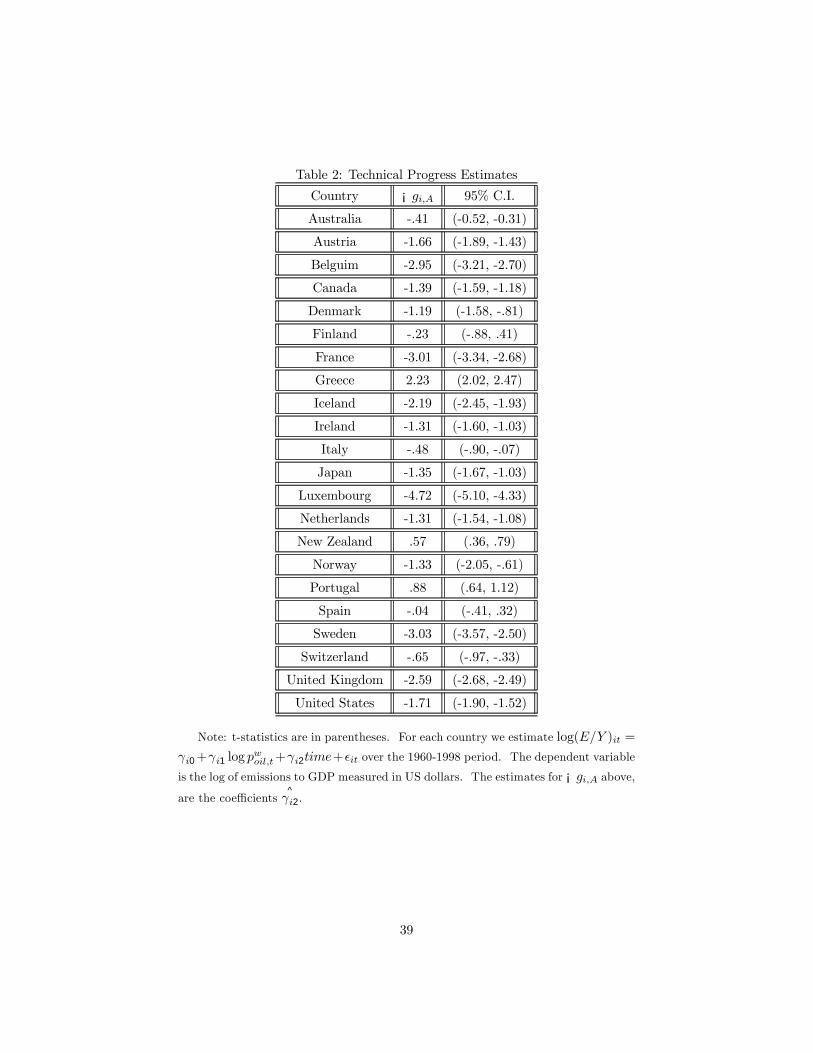
Table 2: Technical Progress Estimates

Country ¡$-.! 95% C.I.

Australia -.41 (-0.52, -0.31)

Austria -1.66 (-1.89, -1.43)

Belguim -2.95 (-3.21, -2.70)

Canada -1.39 (-1.59, -1.18)

Denmark -1.19 (-1.58, -.81)

Finland -.23 (-.88, .41)

France -3.01 (-3.34, -2.68)

Greece 2.23 (2.02, 2.47)

Iceland -2.19 (-2.45, -1.93)

Ireland -1.31 (-1.60, -1.03)

Italy -.48 (-.90, -.07)

Japan -1.35 (-1.67, -1.03)

Luxembourg -4.72 (-5.10, -4.33)

Netherlands -1.31 (-1.54, -1.08)

New Zealand .57 (.36, .79)

Norway -1.33 (-2.05, -.61)

Portugal .88 (.64, 1.12)

Spain -.04 (-.41, .32)

Sweden -3.03 (-3.57, -2.50)

Switzerland -.65 (-.97, -.33)

United Kingdom -2.59 (-2.68, -2.49)

United States -1.71 (-1.90, -1.52)

Note: t-statistics are in parentheses. For each country we estimate log(9:" )-+ =

O-0+O-1 log ,/0-1.++O-20132+@-+ over the 1960-1998 period. The dependent variable

is the log of emissions to GDP measured in US dollars. The estimates for ¡$-.! above,are the coe¢cients

^O-2.

39

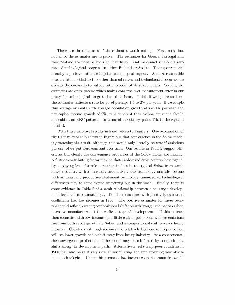
There are three features of the estimates worth noting. First, most but

not all of the estimates are negative. The estimates for Greece, Portugal and

New Zealand are positive and signi�cantly so. And we cannot rule out a zero

rate of technological progress in either Finland or Spain. Taking our model

literally a positive estimate implies technological regress. A more reasonable

interpretation is that factors other than oil prices and technological progress are

driving the emissions to output ratio in some of these economies. Second, the

estimates are quite precise which makes concerns over measurement error in our

proxy for technological progress less of an issue. Third, if we ignore outliers,

the estimates indicate a rate for $! of perhaps 1.5 to 2% per year. If we couple

this average estimate with average population growth of say 1% per year and

per capita income growth of 2%, it is apparent that carbon emissions should

not exhibit an EKC pattern. In terms of our theory, point T is to the right of

point B.

With these empirical results in hand return to Figure 8. One explanation of

the tight relationship shown in Figure 8 is that convergence in the Solow model

is generating the result, although this would only literally be true if emissions

per unit of output were constant over time. Our results in Table 2 suggest oth-

erwise, but clearly the convergence properties of the Solow model are helping.

A further contributing factor may be that unobserved cross country heterogene-

ity is playing less of a role here than it does in the typical Solow framework.

Since a country with a unusually productive goods technology may also be one

with an unusually productive abatement technology, unmeasured technological

di¤erences may to some extent be netting out in the wash. Finally, there is

some evidence in Table 2 of a weak relationship between a country�s develop-

ment level and its estimated $!. The three countries with positively estimated

coe¢cients had low incomes in 1960. The positive estimates for these coun-

tries could re�ect a strong compositional shift towards energy and hence carbon

intensive manufactures at the earliest stage of development. If this is true,

then countries with low incomes and little carbon per person will see emissions

rise from both rapid growth via Solow, and a compositional shift towards heavy

industry. Countries with high incomes and relatively high emissions per person

will see lower growth and a shift away from heavy industry. As a consequence,

the convergence predictions of the model may be reinforced by compositional

shifts along the development path. Alternatively, relatively poor countries in

1960 may also be relatively slow at assimilating and implementing new abate-

ment technologies. Under this scenario, low income countries countries would

40

see a large increase in carbon per capita because of relatively fast growth but

relatively slow progress in adopting new abatement technologies. Together

these four reasons - output convergence, compositional shifts, reduced hetero-

geneity and technology catch up- may explain the strength of our goodness of

�t statistics and the tightness of the relationship depicted in Figure 8

Although the evidence for convergence in Figure 8 seems undeniable, it is

well known that cross-sectional tests such as ours may indicate convergence

while time series tests �nd no such evidence (See for eg. Bernard and Durlauf

1995). Fortunately, in a series of prescient papers John List and a series of

coauthors20 have explored the time series properties of several pollutants to

examine convergence in pollution levels across both states and countries. In

Stracizich and List (2003) the authors examine the convergence properties of

CO2 over a panel of 21 industrial countries from 1960-1997. When the authors

estimate a relationship equivalent to our short regression they �nd evidence

very similar to our OECD regression in column (1). The authors then add a

series of conditioning variables (temperature, energy prices, and the level and

square of per capita income and population density ) to allow for conditional

convergence but have little success. This is perhaps not surprising in light of

our theory since these are not variables determining steady states in the Green

Solow model. Stacizich and List supplement their cross-country regressions

with a time series test of convergence using a panel unit root test. This time-

series test also strongly supports convergence. The authors conclude there is

signi�cant evidence that CO2 emissions per capita have converged. Further

work by Lee and List (2002) and Bulte et al. (2003) employ newer time series

tests or examine new data sources. Overall, their results demonstrate that there

is considerable evidence of convergence in pollution levels across both countries

(for CO2) and across states (for both SO2 and NOx) although convergence may

be stronger over the last 30 years.

20 See List (1999), Lee and List (2002), Strazicich and List (2003), and Bulte, Strazicichand List (2003). This work is largely empirical arguing for a convergence speci�cation byanalogy with the Solow model. Bulte et al. (2003) contains theory that extends the Andreoniand Levinson (2001) model to a dynamic environment to derive a testable equation. Theresulting derivation is however problematic. Equation (5) of Bulte et al (2003), which givesthe balanced growth path level of pollution, produces negative pollution for �nite t (when thereare increasing returns to abatement which is their standard case and necessary to produce theEKC in the model). Pollution goes to negative in�nity as time progresses. When there areconstant returns to abatement the EKC is no longer a prediction and their equation (5) yieldsnegative pollution levels for all t when 6 ' &. These problems seem to have arisen frommapping the strong increasing returns to abatement in the Andreoni and Levinson (2001)model into a model where investment in abatement rises lockstep with aggregate output.

41

Convergence is also apparent in the earlier work of Holtz-Eakin and Selden

(1995). These authors examined whether carbon per capita followed an EKC.

They found that the carbon EKC turned quite late, if at all, at income per capita

levels ranging from 35,000 (1986 US Dollars) to above $8 million per capita

depending on the speci�cation. A key �nding was that the marginal propensity

to emit (the change in emissions per person for a given change in income per

capita) fell with income levels but that overall emissions were forecast to grow.

These �ndings are consistent with the Green Solow model when $! > * + $.

Under these circumstances, convergence in emissions per person still obtains,

but emissions still grow along the balanced growth path.

In total there is considerable evidence of convergence in measures of pollu-

tion emissions. What the Green Solow model o¤ers to this body of work is a

theoretical structure that links the strength of convergence to observable vari-

ables, makes explicit and testable connections between theory and empirical

work, and o¤ers a new method for learning about the growth and environment

relationship.

4 Discussion and Extensions

We have presented a very simple theory linking growth rates, income levels

and environmental quality. In doing so we have made a host of simplifying

assumptions some of which may appear quite limiting. In this section we

discuss these assumptions, provide further empirical evidence supporting our

approach and develop methods for extending our results.

4.1 Sample Selection, Galton�s Fallacy and ! Convergence

Our empirical methods are closely related to those employed in the cross-country

growth literature where variation in cross-country growth rates over some period

of time are explained by initial income plus other controls. The cross-country

growth literature is voluminous and controversial. It started with the work of

Baumol (1986), was formalized and extended by the important contributions

of Barro (1991) and Barro and Sala-i-Martin (1992), and it played an lead role

in Mankiw, Romer and Weil (1992). Durlauf and Quah (1999) provide an

excellent critical review of the empirical literature.

Since our methods are similar, some - but not all - of the criticisms of cross-

country growth regressions are relevant to the estimates we provided here. The

42

earliest critique came from DeLong (1988) who argued that Baumol�s (1986)

original �nding of convergence in productivity levels across 16 currently rich

countries was the result of sample selection and measurement error. Mea-

surement error was a potentially important econometric problem since the data

spanned the 1870 -1979 period, with the quality of the 1870 data quite un-

certain. As DeLong noted measurement error in the estimates of 1870 values

worked towards the convergence �nding. Since our data only spans the 1960-

1998 period we think the measurement error issues discussed by DeLong are

largely irrelevant here.

Sample selection may however be an issue, and DeLong argued that the 16

countries chosen by Baumol were ex post winners who undoubtedly di¤ered

in their productivity levels in earlier years; as a consequence the convergence

�nding was all but guaranteed. Sample selection could be an issue with our

dataset. For example, the convergence we �nd and attribute to the interplay

of diminishing returns and technological progress, could arise from convergence

in environmental policies driven by income convergence across the rich OECD

countries in our sample. While this is a possibility two pieces of evidence work

in our favor. The �rst is that carbon emissions are largely unregulated and

have been largely unregulated for many years. Therefore convergence in carbon

emissions is unlikely to arise from forces causing convergence in environmental

policies amongst the OECD.21

The second piece of evidence is shown in Figure 9 below. Here we follow

DeLong�s advice and extend our sample of rich OECD countries to include all

other countries that as of 1960 were at least as well o¤ as the poorest OECD

member included (Portugal). Extending the sample in this way gives us a

sample of 32 countries; ten of which do not appear in the high income OECD in

1998.22 As shown by Figure 9, the strong convergence properties remain with

the larger sample.

21While some carbon abatement occurs as a joint product of other abatement e¤orts, thetime pro�les for carbon and the set of highly regulated pollutants are very di¤erent.22The additional countries are Venezuela, Uruguay, South Africa, Saudi Arabia, Puerto

Rico, Israel, Hong Kong, Barbardos, Bahamas and Argentina.

43

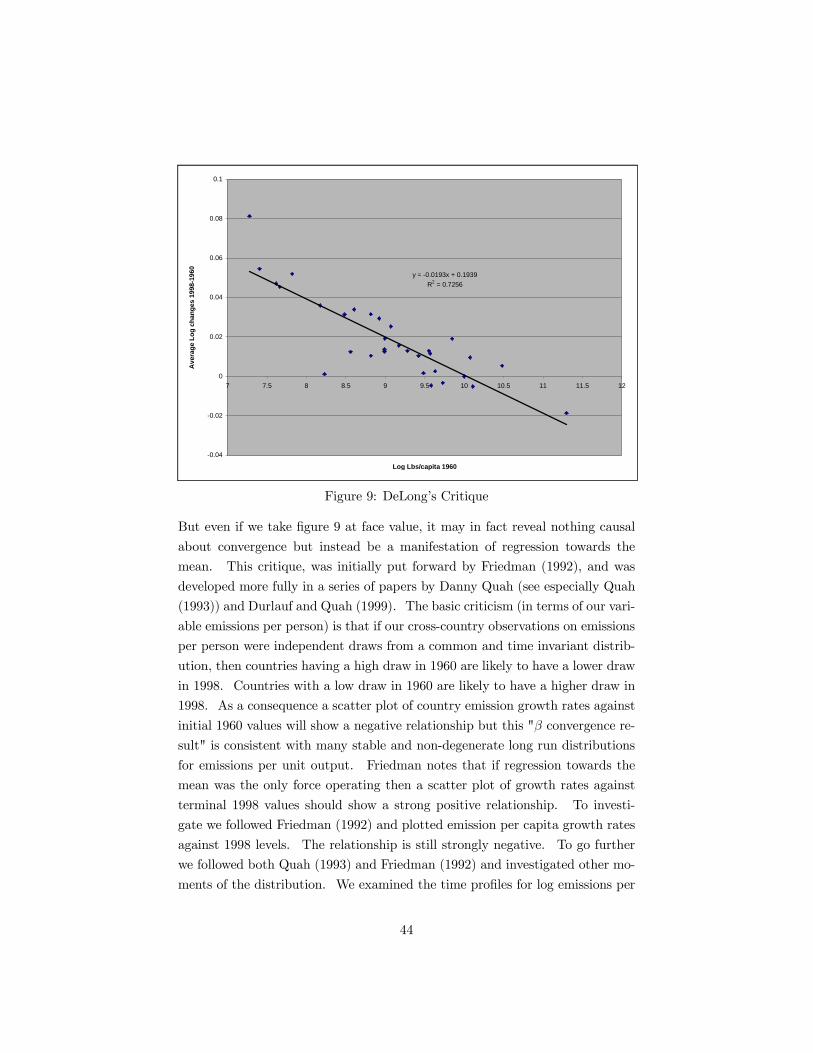
y = -0.0193x + 0.1939R2 = 0.7256

-0.04

-0.02

0

0.02

0.04

0.06

0.08

0.1

7 7.5 8 8.5 9 9.5 10 10.5 11 11.5 12

Log Lbs/capita 1960

Ave

rage

Log

cha

nges

199

8-19

60

Figure 9: DeLong�s Critique

But even if we take �gure 9 at face value, it may in fact reveal nothing causal

about convergence but instead be a manifestation of regression towards the

mean. This critique, was initially put forward by Friedman (1992), and was

developed more fully in a series of papers by Danny Quah (see especially Quah

(1993)) and Durlauf and Quah (1999). The basic criticism (in terms of our vari-

able emissions per person) is that if our cross-country observations on emissions

per person were independent draws from a common and time invariant distrib-

ution, then countries having a high draw in 1960 are likely to have a lower draw

in 1998. Countries with a low draw in 1960 are likely to have a higher draw in

1998. As a consequence a scatter plot of country emission growth rates against

initial 1960 values will show a negative relationship but this "N convergence re-

sult" is consistent with many stable and non-degenerate long run distributions

for emissions per unit output. Friedman notes that if regression towards the

mean was the only force operating then a scatter plot of growth rates against

terminal 1998 values should show a strong positive relationship. To investi-

gate we followed Friedman (1992) and plotted emission per capita growth rates

against 1998 levels. The relationship is still strongly negative. To go further

we followed both Quah (1993) and Friedman (1992) and investigated other mo-

ments of the distribution. We examined the time pro�les for log emissions per

44

person and calculated the point in time variances across the sample. These two

exercises showed a great deal of convergence in the distribution.

In total, these additional checks make us reasonably con�dent that the con-

vergence we �nd in the data is not due to sample selection, measurement error,

or regression towards the mean. The concerns of Durlauf and Quah (1999) and

Durlauf and Johnson (1995) regarding convergence across a very heterogenous

worldwide sample are largely moot here given our select sample of countries.

The additional issues raised by Durlauf and Quah (1999) regarding the inter-

pretation of cross country growth results as tests of new versus old growth the-

ory, the treatment of endogenous regressors, the fragility of estimates, and the

addition of ad hoc regressors to proxy for the free parameters of the production

function would of course be relevant to any extension of our work.

4.2 International Evidence

The starting point for our analysis was three observations drawn from U.S. data:

emissions per unit of output have been falling for lengthy periods of time; these

reductions predate reductions in the absolute level of emissions; and abatement

costs are a relatively small share of overall economic activity. In Table 3 we

present the available evidence from European countries on these same three

statistics for four of the pollutants we considered in Figure 1.

We focus on European evidence because of data limitations. The table

presents summary statistics for the average yearly percentage change in emis-

sions per unit GDP over the 1980-2001 period. As well, where possible, the

table indicates when aggregate emissions peaked but in many cases this is prior

to the start of the sample as indicated by the entry "> 1980". In the last

column we list the country averages for pollution abatement costs as a fraction

of GDP over the 1990-2000 period for these same countries.

There are two remarkable features of the data. The �rst is the massive

reduction in emissions per unit of output over the period. These reductions

are on the order of 4-5% per year for nitrogen oxides, carbon monoxide, and

volatile organic compounds but closer to 10% per year for sulfur. The second is,

of course, the relatively small pollution control costs shown in the last column.

On average these costs are only between 1 and 2% of GDP.

45

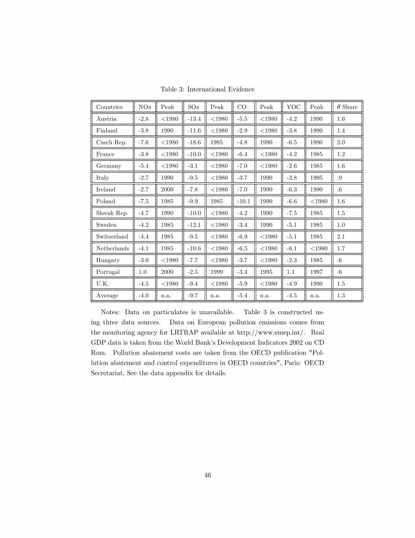
Table 3: International Evidence

Countries NOx Peak SOx Peak CO Peak VOC Peak ; Share

Austria -2.8 !1980 -13.4 !1980 -5.5 !1980 -4.2 1990 1.6

Finland -3.8 1990 -11.6 !1980 -2.9 !1980 -3.8 1990 1.4

Czech Rep. -7.6 !1980 -18.6 1985 -4.8 1990 -6.5 1990 2.0

France -3.8 !1980 -10.0 !1980 -6.4 !1980 -4.2 1985 1.2

Germany -5.4 !1980 -3.1 !1980 -7.0 !1980 -2.6 1985 1.6

Italy -2.7 1990 -9.5 !1980 -3.7 1990 -3.8 1995 .9

Ireland -2.7 2000 -7.8 !1980 -7.0 1990 -6.3 1990 .6

Poland -7.5 1985 -9.9 1985 -10.1 1990 -6.6 !1980 1.6

Slovak Rep. -4.7 1990 -10.0 !1980 -4.2 1990 -7.5 1985 1.5

Sweden -4.2 1985 -12.1 !1980 -3.4 1990 -5.1 1985 1.0

Switzerland -4.4 1985 -9.5 !1980 -6.9 !1980 -5.1 1985 2.1

Netherlands -4.1 1985 -10.6 !1980 -6.5 !1980 -6.1 !1980 1.7

Hungary -3.0 !1980 -7.7 !1980 -3.7 !1980 -2.3 1985 .6

Portugal 1.0 2000 -2.5 1999 -3.4 1995 1.1 1997 .6

U.K. -4.5 !1980 -9.4 !1980 -5.9 !1980 -4.9 1990 1.5

Average -4.0 n.a. -9.7 n.a. -5.4 n.a. -4.5 n.a. 1.3

Notes: Data on particulates is unavailable. Table 3 is constructed us-

ing three data sources. Data on European pollution emissions comes from

the monitoring agency for LRTRAP available at http://www.emep.int/. Real

GDP data is taken from the World Bank�s Development Indicators 2002 on CD

Rom. Pollution abatement costs are taken from the OECD publication "Pol-

lution abatement and control expenditures in OECD countries", Paris: OECD

Secretariat, See the data appendix for details.

46

The table also gives, where possible, the peak year for emission levels. In

many cases these peaks occur before 1980, and with the exception of Portugal

and one pollutant for Ireland, the remaining peaks in emissions occurred in the

1980s or early 1990s. Since emissions are now declining for these pollutants

and countries, this European data o¤ers strong con�rmation that each country

pollutant pair exhibits a time pro�le for emissions roughly consistent with an

EKC.23 We have of course argued that the �rst two features of the data imply

a large role for technological progress in abatement, but rapid technological

progress in abatement, when coupled with the convergence properties of the

Solow model, produce the third feature of the data.

4.3 What is "7?

Aggregate models of economic activity make heroic assumptions to bring into

sharp focus relationships that may otherwise be obscured Our analysis is no

di¤erent. Our use of an aggregate measure for technological progress in both

abatement and goods production surely hides many processes at work in the

economy. Changes in the composition of national output and private consump-

tion, fuel mix changes, and changes in factor quality over time are all partly

responsible for the time pro�le of emissions to GDP that we have observed over

the last �fty years. And many sorts of changes, including regulatory ones, lie

behind what we have called technological progress in abatement. But whether

this is a good or misleading way to think about the growth and environment

relationship does not rest on whether this characterization is literally true, but

whether it helps us identify a key force at work.

Our review of current empirical evidence suggests a key role for technological

progress in abatement. We note that most if not all EKC studies �nd a strong

and persistent time e¤ect driving emissions downward. These time e¤ects

are not small and reduce emissions by signi�cant amounts each year.24 More

direct evidence is contained in studies that decompose the change in pollution23Because, in the words of Andreoni and Levinson, what is now coming down must have

�rst gone up.24The interested reader should take his or her favourite EKC study and conduct the following

experiment. Calculate the number of years it would take for an average developing countryto move from low income to high income status if growth in per capita income were rapid -say 5% per year. Calculate what the implied income gain would mean in terms of reducedemissions/concentrations. Then calculate using the coe¢cient estimate on time in the sameEKC regression the implied reduction in emissions/concentrations that would occur via timerelated e¤ects over this same interval. Compare the magnitude of these two changes. In thecases we have investigated, time related e¤ects are often ten times larger than the changescreated by income growth.

47

emissions into scale, composition and technique e¤ects. For example, Selden et

al. (1999) provide a decomposition of the change in US air pollution emissions

over the 1970 to 1990 period. Using data on 6 criteria pollutants they divide

the change in emissions into scale, composition and three types of technique

e¤ects. For all six criteria pollutants (lead, sulfur dioxide, nitrogen oxide,

volatile organic compounds, carbon monoxide and particulates) reductions in

emissions per unit fuel combusted, and reductions in emissions per unit output

were key in driving emissions downwards. While changes in the composition of

output lowered emissions for some pollutants, it raised them for volatile organic

compounds and carbon monoxide. And while changes in energy intensity and

the mix of energy sources helped lower the emissions of some pollutants, for all

pollutants studied emissions would have risen in the absence of the change in

techniques discussed above.

Related work by Bruvoll and Medin (2003) �nd similar results using Norwe-

gian data. They report that their analysis reveals that "air pollution has not

followed the pace of economic growth. This is mainly due to new technologies";

and that "changes in production structure or composition of energy types have

been of less importance to the development of energy related emissions", p. 42.

Overall these results suggest to us that a large component of the change

in the emissions to output ratio must be technological progress. Composition

changes have not been large enough, technology or technique e¤ects have been

found to be key, and abatement costs are just too small to be largely responsible

for the large reductions in emissions per unit of output experienced.

4.4 Optimization and Functional Forms

To what extent are our assumptions of �xed abatement or savings rates required

for our results? It is well known that allowing for optimal consumption com-

plicates but does not reverse the Solow model�s convergence properties. With

optimal consumption the savings rate now varies over the transition path and

this may hasten or delay the speed of adjustment to the steady state. One

concern may be that optimal abatement could shift over the transition path in

such a way as to rule out the EKC pro�le we derived. To investigate note that if

the optimal E is bounded, then emissions have to fall in the long run if G& > 0.

Therefore, falling emissions and rising environmental quality are guaranteed. In

the short run emissions will at �rst rise as long as the abatement is not initially

too aggressive relative to the pace of growth. Many di¤erent assumptions will

48

generate this result. In our �xed rule case we generated this result by assuming

the initial capital stock E(0) was less than E) . The small initial capital ensured

growth was rapid and this overwhelmed technological progress in abatement.

In an optimizing framework similar forces are at work but we need to add as-

sumptions on abatement (to ensure its growth is not too rapid), consumption

(to make sure output growth is rapid enough initially) and marginal damage (to

control the planner�s response to rising pollution).

One method is to assume marginal damage from emissions is not too high

when E(0) is small so that abatement is not undertaken initially. For example

we could assume the marginal product of abatement is bounded above and the

damage from pollution convex in emissions as in Stokey (1998) or Brock and

Taylor (2003a). In this situation the �rst unit of emissions has zero marginal

damage while abatement has a �nite cost (determined by the shadow value

of capital). These authors show emissions at �rst rise only to be o¤set by

abatement or a combination of abatement plus technological progress in the

future.

Alternatively, we could let the abatement function satisfy Inada type con-

ditions so that abatement is always undertaken, but then adopt assumptions

to ensure that sacri�ces in consumption are not too costly (so growth is ini-

tially rapid) and pollution not too damaging (to make policy responses weak).

In short many sets of reasonable assumptions on abatement and utility will

generate the result that pollution can at �rst rise with growth. Assuming suf-

�ciently strong technological progress in abatement ensures that pollution will

fall eventually.

A �nal concern of readers may be our use of a Cobb-Douglas aggregator for

output. Although this functional form is commonly used in growth theory and

elsewhere, it is important to understand its limitations. Its bene�t to us out-

weighed its costs because it allowed us to derive simple closed form solutions for

quantities of interest. In many cases our results carry through although they

are more di¢cult to prove and less transparent to the reader. For example,

our key result that an EKC relationship arises from the interplay of diminish-

ing returns and technological progress in abatement remains true. To verify

consider the dynamics of environmental quality X and income per capita with

a general intensive production function D(E). Assume D(E) satis�ed the Inada

conditions, and write the dynamic system for E and A as:

49

²E = !D(E)[1¡ ;]¡ [# + *+ $]E (26)²A = 50 exp[G&0]D(E)¡ BA (27)

where 50 ? 0 and G& > 0. To show the environment must at �rst worsen

evaluate 27 at 0 = 0. At 0 = 0 the environment is initially pristine, A(0) = 0,

and the initial capital stock is not zero, E(0) ? 0F Equation 27 shows the

environment must at �rst worsen. A has to be growing at least initially. To

examine the rest of the transition path recall E(0) is increasing in time until it

reaches E¤. We can use this fact to bound the path for A noting:

²A = 50 exp[G&0]D(E)¡ BA >

²A = 50 exp[G&0]D(E¤)¡ BA (28)

For any 0 ? 0, A(0) must be below the solution to the ordinary di¤erential

equation²A = 50 exp[G&0]D(E¤) ¡ BA, A(0) = 0. This ordinary di¤erential

equation has a closed form solution showing A(0) tends to zero as t goes to

in�nity. Using the inequality in 28 we conclude A must at �rst rise, but then

fall as before. Proving a similar result for 9(0) is left to the reader. The EKC

prediction of the model is not limited to our Cobb-Douglas formulation.

5 Conclusion

This paper presented a simple growth and pollution model to investigate the

relationship between economic growth and environmental outcomes. A recent

and very in�uential line of research centered on the empirical �nding of an EKC

has, for the last ten years, dominated the way that economists and policymakers

think about the growth and environment interaction. Numerous empirical

researchers have sought to validate or contradict the original EKC �ndings by

Grossman and Krueger (1994, 1995), while theorists have contributed to this

explosion of research by presenting a myriad of possible explanations for the

empirical result.

This paper makes three contributions to this line of enquiry. First and

foremost it suggests that the most important empirical regularity found in the

environment literature - the EKC - and the most in�uential model employed

in the macro literature - the Solow model - are intimately related. While one

hesitates to see "Solow everywhere", we have argued that the forces of dimin-

50

ishing returns and technological progress identi�ed by Solow as fundamental to

the growth process, may also be fundamental to the EKC �nding.

In support of our argument we marshalled several pieces of evidence. We

presented evidence that the U.S. emission to output ratio has fallen at a roughly

constant rate for almost 50 years; that this reduction predates the peak of

emissions; and that abatement expenditures while growing since the early 1970s

have remained a fairly constant fraction of economic activity. These data are

in many cases inconsistent with current explanations for the EKC.

Our second contribution was to develop a simple extension of the Solow

model where the interplay of diminishing returns to capital formation and tech-

nological progress in abatement produced a time pro�le for emissions, abatement

costs, and emissions to output ratios that are in accord with U.S. data. We also

argued that this model could provide a natural explanation for the sometimes

confusing and heterogenous results found in the empirical literature.

Finally we developed an empirical methodology that �owed very naturally

from our model. By exploiting known results in the macro literature we de-

veloped a simple estimating equation predicting convergence in emissions per

capita across countries. The model produced several testable restrictions and

led to the estimation of key parameters. While we view our empirical work

as preliminary, it lends further support to our view that the same ongoing dy-

namic processes responsible for income growth and convergence are also at play

in determining the EKC �nding and emission convergence. The evidence for

convergence is quite strong, and well in accord with the theoretical predictions

of the Green Solow Model.

The very simplicity of our model calls out for future work to qualify, elab-

orate or perhaps refute our thesis. The model is singularly successful in iden-

tifying technological progress in abatement as a potential key to much of the

income and pollution data, but no theory of innovation nor optimal regulation

was provided. Our formulation is consistent with a world where governments

gradually tighten emission standards over time, but we can only speculate as to

whether this gradual march forward in regulation is caused by income growth

and whether gradually tightening standards are the impetus for ongoing techni-

cal improvements in abatement. Our empirical work, as we state, is preliminary

and our method of estimating technological progress in abatement crude. Mov-

ing forward on both empirical and theoretical fronts is surely a worthy goal for

future research.

51

6 Appendix

6.1 Constant costs and rising standards

It proves useful to adopt a speci�c abatement production function and consider

the �rm�s problem. To that end, let the intensive abatement production func-

tion be given by 7(;) = [1¡ ;]2 where P ? 1. Assume the government imposesa technology restriction requiring emissions per unit of output not exceed M(0);

that is, 9(0):" (0) · M(0). If �rm�s rent capital at rate 6, hire labor at the wage

<, and face the technology standard M(0), then the �rm�s problem becomes one

of maximizing pro�ts by choice of labor, capital and abatement inputs

Q7Rf$.1.3g

¦ = " ¡<)¡ 6& (29)

!F0F" = (1¡ ;)% (&'()) (30)

9 = ­[1¡ ;]2%' (31)

9:" · M (32)

Since abatement is costly in terms of foregone output �rms will only just meet

the technological standard. Using this information we can substitute the con-

straints into the objective to rewrite the �rm�s problem as simply

Q7Rf$.1g

¦ = (M:­)1*("¡1) % (&'())¡<)¡ 6&

which is just a straightforward problem of input choice. The �rm�s allocation

of labor and capital to abatement is determined by the technological standard.

Algebra shows

(M:­) = (1¡ ;)("¡1) (33)

which solves for the intensity of abatement implicitly. Note if M = ­, no

abatement is necessary and ; = 0, but as standards tigten M falls and ; must rise.

Suppose the technology standard is tightened slowly over time. Di¤erentiating

with respect to time we obtain:

¢M

M+ $! = (@¡ 1) 4

40ln(1¡ ;)

52

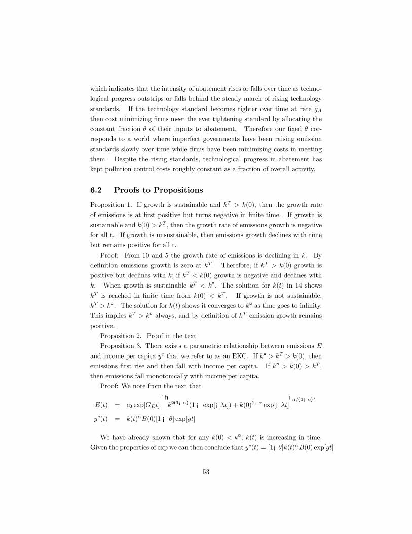
which indicates that the intensity of abatement rises or falls over time as techno-

logical progress outstrips or falls behind the steady march of rising technology

standards. If the technology standard becomes tighter over time at rate $!then cost minimizing �rms meet the ever tightening standard by allocating the

constant fraction ; of their inputs to abatement. Therefore our �xed ; cor-

responds to a world where imperfect governments have been raising emission

standards slowly over time while �rms have been minimizing costs in meeting

them. Despite the rising standards, technological progress in abatement has

kept pollution control costs roughly constant as a fraction of overall activity.

6.2 Proofs to Propositions

Proposition 1. If growth is sustainable and E) ? E(0), then the growth rate

of emissions is at �rst positive but turns negative in �nite time. If growth is

sustainable and E(0) ? E) ' then the growth rate of emissions growth is negative

for all t. If growth is unsustainable, then emissions growth declines with time

but remains positive for all t.

Proof: From 10 and 5 the growth rate of emissions is declining in E. By

de�nition emissions growth is zero at E) . Therefore, if E) ? E(0) growth is

positive but declines with E; if E) > E(0) growth is negative and declines with

E. When growth is sustainable E) > E¤. The solution for E(0) in 14 showsE) is reached in �nite time from E(0) > E) . If growth is not sustainable,

E) ? E¤. The solution for E(0) shows it converges to E¤ as time goes to in�nity.This implies E) ? E¤ always, and by de�nition of E) emission growth remainspositive.

Proposition 2. Proof in the text

Proposition 3. There exists a parametric relationship between emissions 9

and income per capita C% that we refer to as an EKC. If E¤ ? E) ? E(0), thenemissions �rst rise and then fall with income per capita. If E¤ ? E(0) ? E) ,

then emissions fall monotonically with income per capita.

Proof: We note from the text that

9(0) = 50 exp[G&0]

·hE¤(1¡()(1¡ exp[¡J0]) + E(0)1¡( exp[¡J0]

i(*(1¡()¸

C%(0) = E(0)(((0)[1¡ ;] exp[$0]

We have already shown that for any E(0) > E¤, E(0) is increasing in time.Given the properties of exp we can then conclude that C%(0) = [1¡;]E(0)(((0) exp[$0]

53

is strictly increasing in time when the conditions of the proposition are met. This

allows us to invert and obtain 0 = S(C%) where S0 ? 0. Substitute for time

in 9(0). Now di¤erentiate this parametric function 9(S(C%)) with respect to

C% to obtain 90(S(C%))S0(C%). Note that if E¤ ? E) ? E(0) then 90(S(C%)) ispositive for 0 > I , zero at 0 = I , and negative for 0 ? I . S0(C%) is alwaysstrictly positive and hence emissions at �rst rise and then fall with income per

capita. If E¤ ? E(0) ? E) ,then 90(S(C%)) is always negative. This implies

90(S(C%))S0(C%) is always negative as required.

6.3 Derivation of Estimating Equation

Start with the capital accumulation equation in 5 and use the following log

linearization

²E

E= !E(¡1[1¡ ;]¡ [# + *+ $] (34)

»= ^E]¡ [# + *+ $] (35)

^E = log E(0)¡ log E¤ (36)

Rearrange and use the de�nition of E¤ and J to obtain the simpler form

²E

E= ¡(1¡ H)[*+ $ + #]

^E = ¡J

^E (37)

where we have used the fact that²E is zero at E¤. Note that

^E = log[E(0):E¤]

and the left hand side of 37 is just the time derivative of log E(0)F To change

this di¤erential equation in log E(0) to one over C(0) use C = (1¡ ;)E( and thenrewrite it out more completely as

4

40[log C(0)] = ¡J log C(0) + J log C¤ (38)

This equation is easily solved to �nd

log C(0) = log C(0)2¡4+ + log C¤[1¡ 2¡4+] (39)

where C(0) is income per e¤ective worker at 0 = 0F Evaluate 39 at I and

I ¡L . Note I ¡L is our initial period and corresponds to 0 = 0, since C(0)

54

is period I ¡L income per e¤ective worker. Doing so we obtain

log C(I )¡ log C(I ¡L) = ¡ log[C(I ¡L):C¤][1¡ 2¡4, ] (40)

Note that income per e¤ective worker is related to income per worker by

C(0) = C%(0):((0) where ((0) is the index of labor augmenting technological

progress. Making these substitutions leads to

log C%(I )¡ log C%(I ¡L) = L$¡ log[C%(I ¡L):((I ¡L)C¤][1¡ 2¡4, ] (41)

Divide both sides by N to obtain the average log changes over the period

and rearrange slightly to obtain

log[C%(I ):C%(I ¡L)]L

=

·$ + log((I ¡L) [1¡ 2¡4, ]

L+ log[C¤]

[1¡ 2¡4, ]L

¸¡ log[C%(I ¡L)] [1¡ 2¡4, ]

L

which is reported in 22 where the constant b represents the �rst three terms in

brackets.

55

7 Data

We have obtained our data from several sources. Data on carbon emissions,

carbon per capita, carbon per dollar GDP, population size, and investment as a

share of GDP was obtained from the World Bank Development Indicators 2002

available on CD-ROM. The data in Figure 7 is drawn from this source. The

countries that appear in Figure 7 are: Afghanistan, Albania, Algeria, Angola,

Antigua and Barbuda, Argentina, Australia, Austria, Bahamas, Bahrain, Bar-

bados, Belgium, Belize, Benin, Bolivia, Brazil, Brunei, Bulgaria, Burkina Faso,

Cambodia, Cameroon, Canada, Cape Verde, Chad, Chile, China, Colombia,

Congo Dem. Rep.,Congo Rep., Costa Rica, Cote d�Ivoire, Cuba, Cyprus, Den-

mark, Djibouti, Dominica, Dominican Republic, Ecuador, Egypt, Arab Rep.,El

Salvador, Equatorial Guinea, Ethiopia, Fiji, Finland, France, French Polyne-

sia, Gabon, Gambia, Ghana, Greece, Greenland, Grenada, Guam, Guatemala,

Guinea, Guinea-Bissau, Guyana, Haiti, Honduras, Hong Kong, China, Hun-

gary, Iceland, India, Indonesia, Iran, Islamic Rep., Iraq, Ireland, Israel, Italy,

Jamaica, Japan, Jordan, Kenya, Korea, Dem. Rep., Korea, Rep., Kuwait,

Lao PDR, Lebanon, Liberia, Libya, Luxembourg, Macao, China, Madagascar,

Mali, Malta, Mauritania, Mauritius�Mexico, Mongolia, Morocco, Mozambique,

Myanmar, Nepal, Netherlands, New Caledonia, New Zealand, Nicaragua, Niger,

Nigeria, Norway, Papua New Guinea, Paraguay, Peru, Philippines, Poland, Por-

tugal, Puerto Rico, Qatar, Romania, Samoa,Sao Tome and Principe, Saudi Ara-

bia, Senegal,Sierra Leone, Singapore, Solomon Islands, South Africa, Spain,Sri

Lanka�St. Lucia,St. Vincent and the Grenadines, Sudan, Suriname, Sweden,

Switzerland, Syrian Arab, Republic, Thailand, Togo, Tonga, Trinidad and To-

bago, Tunisia, Turkey, Uganda, United Arab Emirates, United Kingdom, United

States, Uruguay, Venezuela, RB,Virgin Islands (U.S.).

Data on US emissions of the criteria pollutants graphed in Figures 1 and 2

come from the US E.P.A. The long series of historical data presented in the

�gures is taken from the EPA�s 1998 report National Pollution Emission Trends,

available at http://www.epa.gov/ttn/chief/trends/trends.98

Data on European pollution emissions given in Table 3 comes from the mon-

itoring agency for LRTRAP available at http://www.emep.int/.

Data on pollution abatement costs came from the 1996 and 2003 OECD

publication Pollution Abatement and Control Expenditures in OECDCountries,

Paris: OECD Secretariat. Since this data is di¢cult to get we have given the

exact method of construction and the data used in the table below.

56

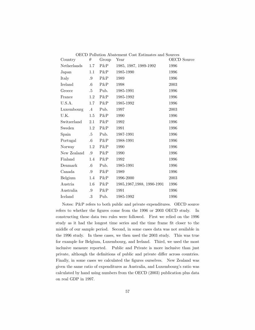
OECD Pollution Abatement Cost Estimates and SourcesCountry ; Group Year OECD Source

Netherlands 1.7 P&P 1985, 1987, 1989-1992 1996

Japan 1.1 P&P 1985-1990 1996

Italy .9 P&P 1989 1996

Ireland .6 P&P 1998 2003

Greece .5 Pub. 1985-1991 1996

France 1.2 P&P 1985-1992 1996

U.S.A. 1.7 P&P 1985-1992 1996

Luxembourg .4 Pub. 1997 2003

U.K. 1.5 P&P 1990 1996

Switzerland 2.1 P&P 1992 1996

Sweden 1.2 P&P 1991 1996

Spain .5 Pub. 1987-1991 1996

Portugal .6 P&P 1988-1991 1996

Norway 1.2 P&P 1990 1996

New Zealand .9 P&P 1990 1996

Finland 1.4 P&P 1992 1996

Denmark .6 Pub. 1985-1991 1996

Canada .9 P&P 1989 1996

Belgium 1.4 P&P 1996-2000 2003

Austria 1.6 P&P 1985,1987,1988, 1990-1991 1996

Australia .9 P&P 1991 1996

Iceland .3 Pub. 1985-1992 1996

Notes: P&P refers to both public and private expenditures. OECD source

refers to whether the �gures come from the 1996 or 2003 OECD study. In

constructing these data two rules were followed. First we relied on the 1996

study as it had the longest time series and the time frame �t closer to the

middle of our sample period. Second, in some cases data was not available in

the 1996 study. In these cases, we then used the 2003 study. This was true

for example for Belgium, Luxembourg, and Ireland. Third, we used the most

inclusive measure reported. Public and Private is more inclusive than just

private, although the de�nitions of public and private di¤er across countries.

Finally, in some cases we calculated the �gures ourselves. New Zealand was

given the same ratio of expenditures as Australia, and Luxembourg�s ratio was

calculated by hand using numbers from the OECD (2003) publication plus data

on real GDP in 1997.

57

8 References

Aghion, P. and P. Howitt (1998), Endogenous Growth Theory, MIT Press,

Cambridge, MA.

Andreoni, J. and A. Levinson (2001), "The Simple Analytics of the Envi-

ronmental Kuznets Curve", Journal of Public Economics, 80:269-86.

Barbier, E.B. (1997), "Introduction to the environmental Kuznets curve spe-

cial issue", Environment and Development Economics 2, 369-381.

Barro, R.J. (1991), "Economic Growth in a Cross Section of Countries",

Quarterly Journal of Economics, 106, 407-443.

Barro, R.J. and X. Sala-i-Martin (1992), "Convergence across States and

Regions", Brookings Papers on Economic Activity 1, 107-182.

Baumol, W. (1986), "Productivity Growth, Convergence andWelfare", Amer-

ican Economic Review, Dec. 76, 1072-85.

Bernard, A.B. and S.N. Durlauf (1995), "Convergence in International Out-

put", Journal of Applied Econometrics, Vol. 10, 97-108.

Bovenberg, A.L. and S. Smulders (1995), "Environmental Quality and pol-

lution augmenting technological change in a two sector endogenous growth

model", Journal of Public Economics, 57, 369-391.

Brock, W.A. and M. Scott Taylor, (2003a), "The Kindergarten Rule of Sus-

tainable Growth", NBER working paper no. 9597, Cambridge, MA. Revised

and retitled as "Economic Growth and the Environment: Matching the Styl-

ized Facts", University of Wisconsin, Social Science Research Institute working

paper No. 2003-16 (August).

Brock, W.A. and M. S. Taylor (2003b), "Economic Growth and the Envi-

ronment: A Review of Theory and Empirics", prepared for the Handbook of

Economic Growth, S. Durlauf and P. Aghion eds. North Holland.

Bruvoll, A. H. Medin (2003), "Factors behind the environmental Kuznets

curve: a decomposition of the changes in air pollution", Environmental and

Resource Economics, 24, 27-48.

Bulte, E., J.A. List and M.C. Strazicich (2003), Regulatory Federalism and

the Distribution of Air Pollutant Emissions", Working paper University of Mary-

land.

Copeland, B.R. and M.S. Taylor (1994), "North-South Trade and the Global

Environment", Quarterly Journal of Economics, 109:755-87.

Copeland, B.R. and M. S. Taylor (2004), "Trade, Growth and the Environ-

ment", Journal of Economic Literature, March, 7-71.

58

Copeland, B.R. and M. S. Taylor (2003), Trade and the Environment: The-

ory and Evidence, Princeton University Press, Princeton, NJ,.

DeLong, J.B., (1988), "Productivity Growth, Convergence, and Welfare:

Comment", American Economic Review, Vol. 78, No. 5, 1138-1154.

Dewey, S.H. (2000), Don�t Breathe the Air: Air Pollution and U.S. Environ-

mental Politics: 1945-1970, No. 16, Environmental History Series, D.L. Flores,

editor, Texas A&M publisher, College Station, TX.

Durlauf, S.N. and P.A. Johnson, (1995), "Multiple Regimes and Cross-

Country Growth Behaviour", Journal of Applied Econometrics, Vol. 10, 365-

384.

Durlauf, S. and D. Quah, (1999), "The New Empirics of Economic Growth",

Handbook of Macroeconmics, North Holland, J. Taylor and M. Woodford eds.

Friedman, M. (1992), "Do Old Fallacies Ever Die?", Journal of Economic

Literature, Vol. XXX, Dec. 2129-2132.

Grossman, G.M. and A.B. Krueger (1994), "Environmental Impacts of a

North American Free Trade Agreement" in P. Garber (Editor) The US-Mexico

Free Trade Agreement, MIT Press, Cambridge MA.

Grossman, G.M. and A.B. Krueger (1995), "Economic growth and the envi-

ronment", Quarterly Journal of Economics, 110, 353-377.

Harbaugh, W., A.M. Levinson, and D.M. Wilson (2002), "Reexamining the

empirical evidence for an environmenal Kuznets curve", Review of Economics

and Statistics, 84, 541-551.

Holtz-Eakin, D. and T.M. Selden (1995), "Stoking the �res? CO2 emissions

and economic growth", Journal of Public Economics, 57, 85-101.

Lee, J. and J.A. List (2002), "Examining Trends of Criteria Air Pollutants:

Are the e¤ects of government intervention transitory", mimeo June.

List, J.A. (1999), "Have Air Pollutant Emissions converged amongst US

Regions? Evidence from Unit root Tests", Southern Economic Journal 66, 144-

155.

List, J.A. and C.A. Gallet, (1999), "The environmental Kuznets curve: does

one size �t all?", Ecological Economics, 31, 409-423.

Lopez, R. (1994). "The Environment as a Factor of Production: the ef-

fects of Economic growth and trade liberalization", Journal of Environmental

Economics and Management 27:163-84.

Mankiw, N.G., D. Romer and D.N. Weil (1992), "A Contribution to the

Empirics of Economic Growth", Quarterly Journal of Economics 107, 407-438.

59

Quah, D. (1993), "Galton�s Fallacy and Tests of the Convergence Hypothe-

sis", Scandinavian Journal of Economics, 95, 427-443.

Selden, T.M., A.S. Forrest, J.E. Lockhart (1999), "Analyzing reductions in

U.S. air pollution emissions: 1970 to 1990", Land Economics, 5,1-21.

Solow, R.M.(1956) "A Contribution to the Theory of Economic Growth",

Quarterly Journal of Economics, LXX, 65-94.

Stern, D.I., (2003), "The Rise and Fall of the Environmental Kuznets Curve",

Rensselaer Polytechnic Institute, Working Paper No. 0302, October.

Stern, D.I. and M.S. Common (2001), "Is there an environmental Kuznets

curve for sulfur?" Journal of Environmental Economics and Management, 41,

162-178.

Stokey, N., (1998), "Are there Limits to Growth", International Economic

Review, vol. 39, No. 1, 1-31.

Strazicich, M. C. and John List (2003), "Are CO2 Emission levels converge-

ing among Industrial coutries", Environmental and Development Economics,

24, 263-271, 2003.

Xepapadeas, A. (2003), "Economic Growth and the Environment", in prepa-

ration for the Handbook of Environmental Economics, J. Vincent and Karl

Goran Maler eds.

Vogan, C.R. (1996) "Pollution Abatement and Control Expenditures:1972-

94", Survey of Current Business, Sept. 48-67.

60