The Theory Of Demand

1

The TheoryOf Demand

Chapter 5

2

Chapter Five Overview

1. Individual Demand Curves

2. Income and Substitution Effects & the Slope of Demand

• Applications: The Work-Leisure Trade-off Consumer Surplus

4. Constructing Market Demand

1. Individual Demand Curves

2. Income and Substitution Effects & the Slope of Demand

• Applications: The Work-Leisure Trade-off Consumer Surplus

4. Constructing Market Demand

Chapter Five

3

Chapter Five Overview

The Effects of a Change in Price• Optimal Choice• Demand Curve

The Effects of a Change in Price• Optimal Choice• Demand Curve

Chapter Five

5

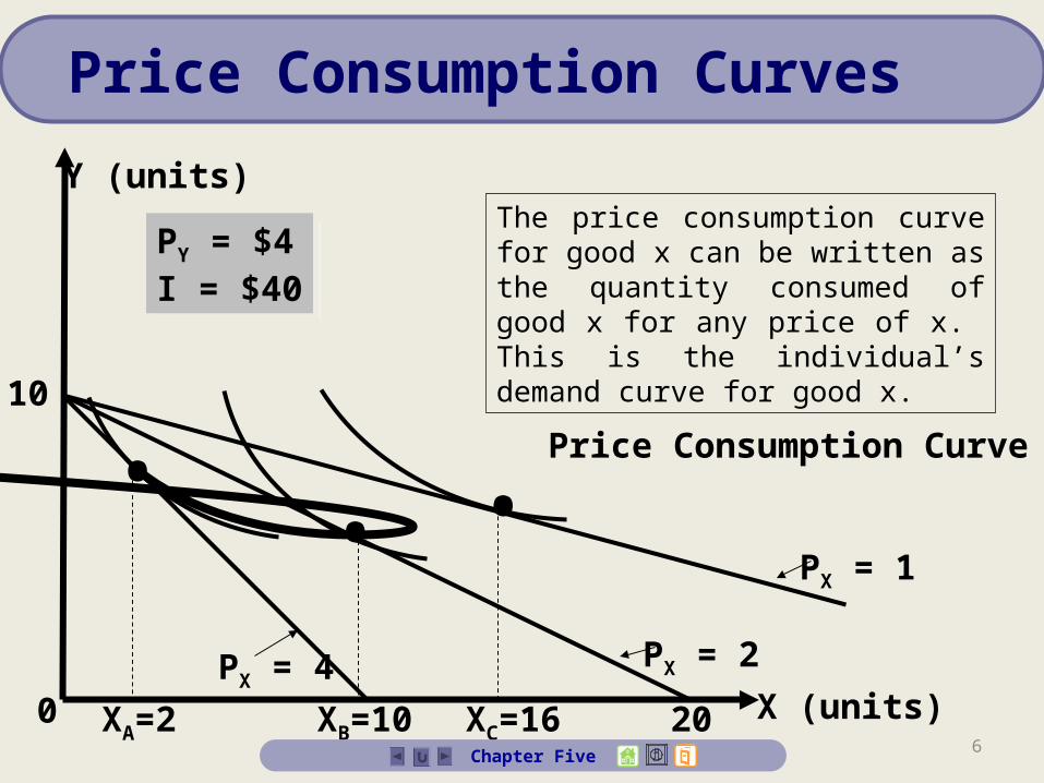
Is the set of optimal baskets for every possible price of good x, holding all other prices and income constant.

The Price Consumption Curve of Good X:The Price Consumption Curve of Good X:

Chapter Five

Individual Demand Curves

6

Y (units)

X (units)0PX = 4 PX = 2

PX = 1

XA=2 XB=10 XC=16

•• •

10

PY = $4I = $40

PY = $4I = $40

Price Consumption Curve

20

The price consumption curve for good x can be written as the quantity consumed of good x for any price of x. This is the individual’s demand curve for good x.

Chapter Five

Price Consumption Curves

7

X

PX

XA XB XC

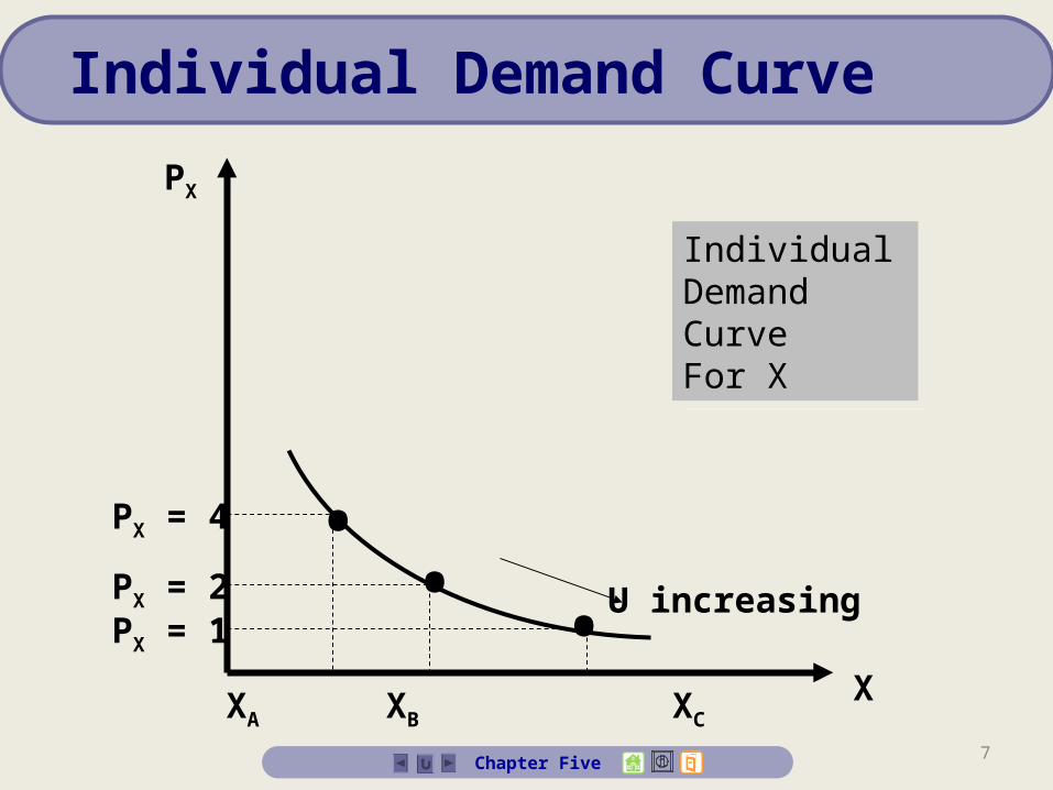
Individual Demand CurveFor X

Individual Demand CurveFor X

PX = 4

PX = 2PX = 1

••

• U increasing

Chapter Five

Individual Demand Curve

8

The consumer is maximizing utility at every point along the demand curve

The marginal rate of substitution falls along the demand curve as the price of x falls (if there was an interior solution).

As the price of x falls, it causes the consumer to move down and to the right along the demand curve as utility increases in that direction.

The demand curve is also the “willingness to pay” curve – and willingness to pay for an additional unit of X falls as more X is consumed.

Chapter Five

Individual Demand Curve

9

Algebraically, we can solve for the individual’s demand using the following equations:

1. pxx + pyy = I2. MUx/px = MUy/py – at a tangency.

(If this never holds, a corner point may be substituted where x = 0 or y = 0)

Algebraically, we can solve for the individual’s demand using the following equations:

1. pxx + pyy = I2. MUx/px = MUy/py – at a tangency.

(If this never holds, a corner point may be substituted where x = 0 or y = 0)

Chapter Five

Demand Curve for “X”

10

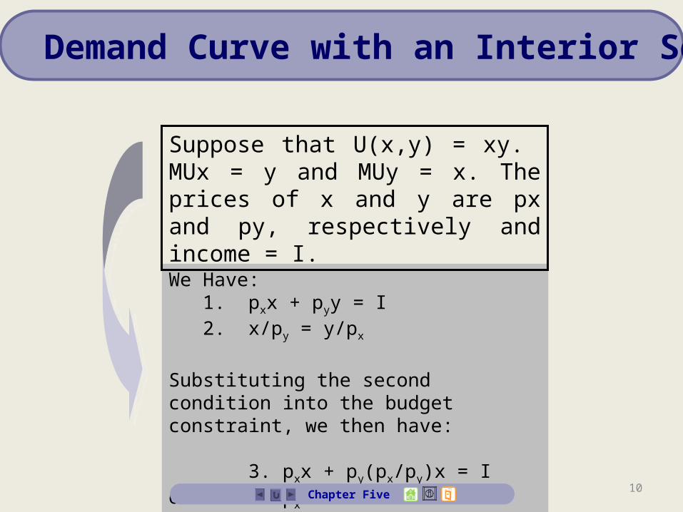
We Have: 1. pxx + pyy = I2. x/py = y/px

Substituting the second condition into the budget constraint, we then have:

3. pxx + py(px/py)x = I or…x = I/2px

We Have: 1. pxx + pyy = I2. x/py = y/px

Substituting the second condition into the budget constraint, we then have:

3. pxx + py(px/py)x = I or…x = I/2px

Chapter Five

Demand Curve with an Interior Solution

Suppose that U(x,y) = xy. MUx = y and MUy = x. The prices of x and y are px and py, respectively and income = I.

11Chapter Five

Change in Income & Demand

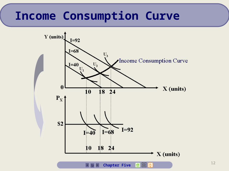
The income consumption curve of good x is the set of optimal baskets for every possible level of income.

We can graph the points on the income consumption curve as points on a shifting demand curve.

The income consumption curve of good x is the set of optimal baskets for every possible level of income.

We can graph the points on the income consumption curve as points on a shifting demand curve.

12Chapter Five

Income Consumption Curve

13

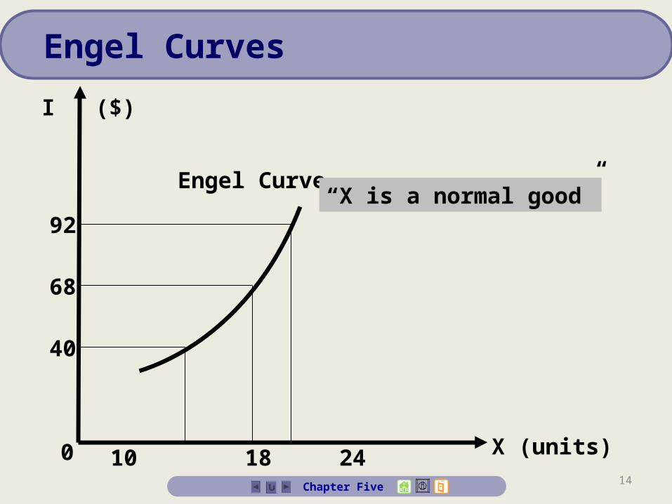
The income consumption curve for good x also can be written as the quantity consumed of good x for any income level. This is the individual’s Engel Curve for good x. When the income consumption curve is positively sloped, the slope of the Engel Curve is positive.

Chapter Five

Engel Curves

14

X (units)0

92

68

40

10 18 24

Engel Curve

Chapter Five

I ($)

“X is a normal good”“X is a normal good”

Engel Curves

15

• If the income consumption curve shows that the consumer purchases more of good x as her income rises, good x is a normal good.

• Equivalently, if the slope of the Engel curve is positive, the good is a normal good.

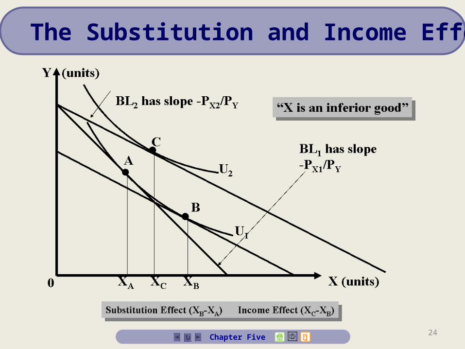
• If the income consumption curve shows that the consumer purchases less of good x as her income rises, good x is an inferior good.

• Equivalently, if the slope of the Engel curve is negative, the good is an inferior good.

Chapter Five

Definitions of Goods

16

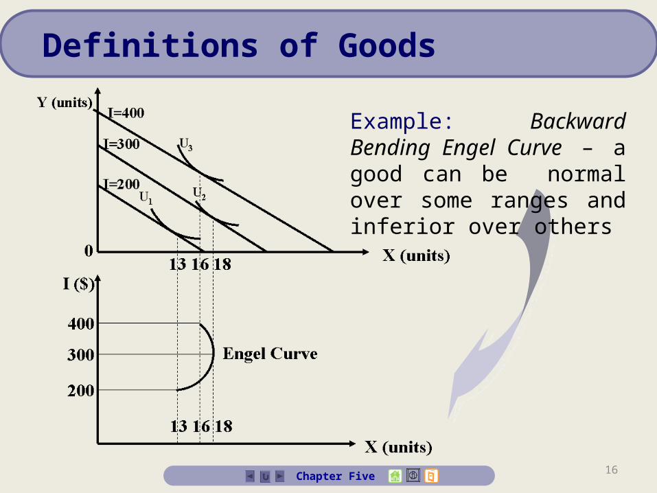
Example: Backward Bending Engel Curve – a good can be normal over some ranges and inferior over others

Chapter Five

Definitions of Goods

17Chapter Five

Impact of Change in the Price of a Good

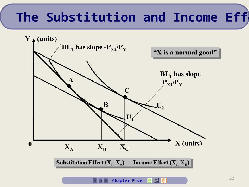
• Substitution Effect: Relative change in price affects the amount of good that is bought as consumer tries to achieve the same level of utility

• Income Effect: Consumer’s purchasing power changes and affects the consumer in a way similar to effect of a change in income

18

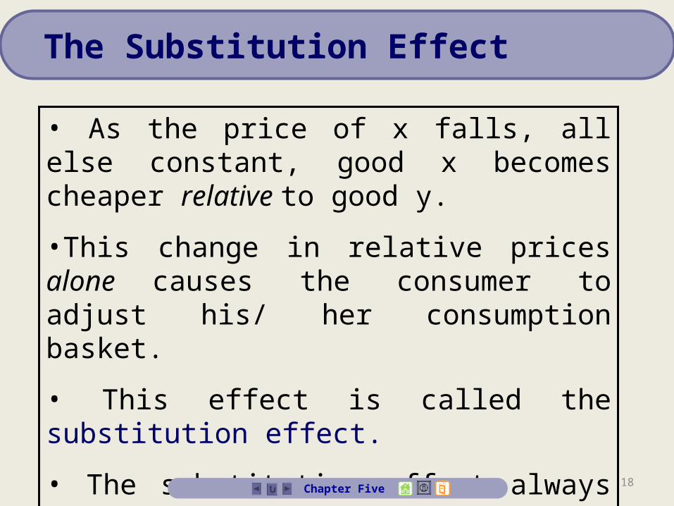
• As the price of x falls, all else constant, good x becomes cheaper relative to good y.

•This change in relative prices alone causes the consumer to adjust his/ her consumption basket.

• This effect is called the substitution effect.

• The substitution effect always is negative.

• Usually, a move along a demand curve will be composed of both effects.

Chapter Five

The Substitution Effect

19Chapter Five


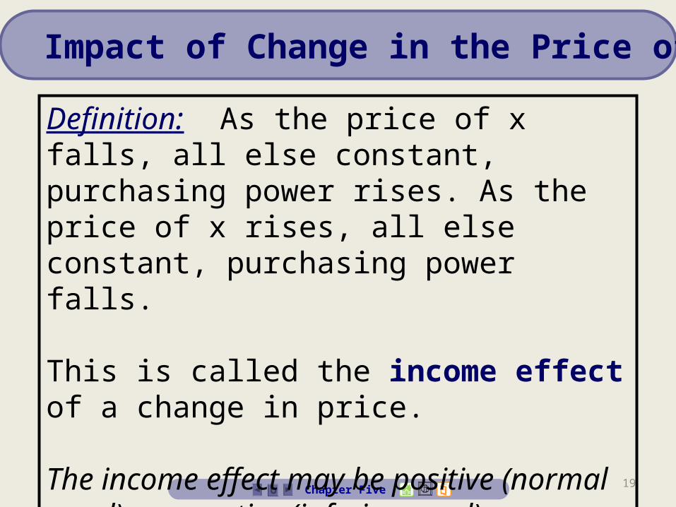
Definition: As the price of x falls, all else constant, purchasing power rises. As the price of x rises, all else constant, purchasing power falls.

This is called the income effect of a change in price.

The income effect may be positive (normal good) or negative (inferior good).

20Chapter Five


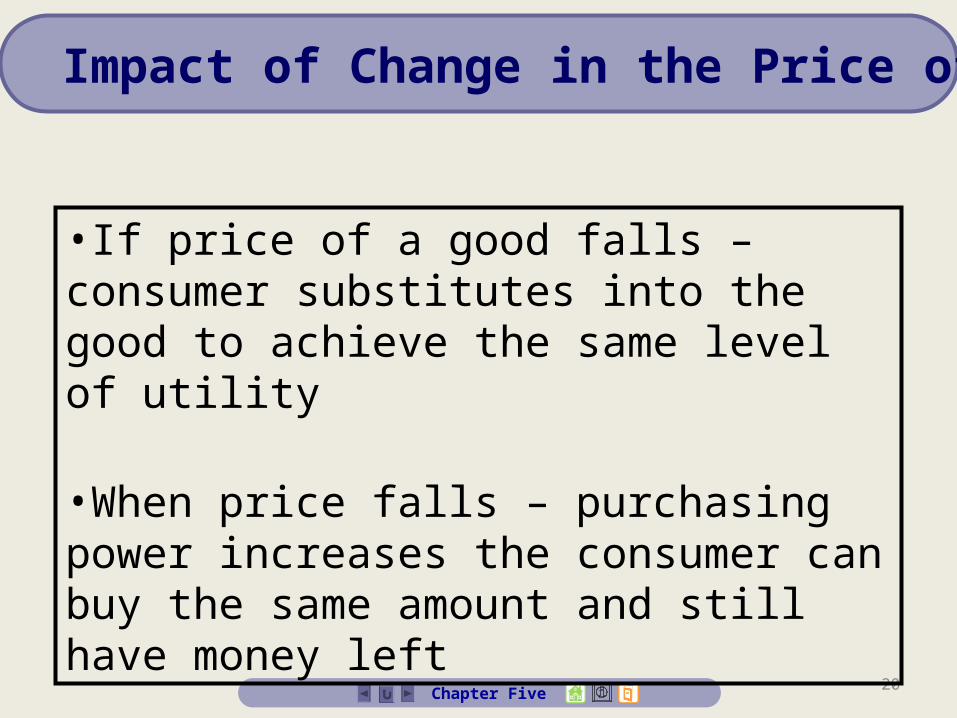
•If price of a good falls – consumer substitutes into the good to achieve the same level of utility

•When price falls – purchasing power increases the consumer can buy the same amount and still have money left

YC

loth

ing

XFood

A C

B

XA XCXB

BL1 BL2

BLd

U1

U2

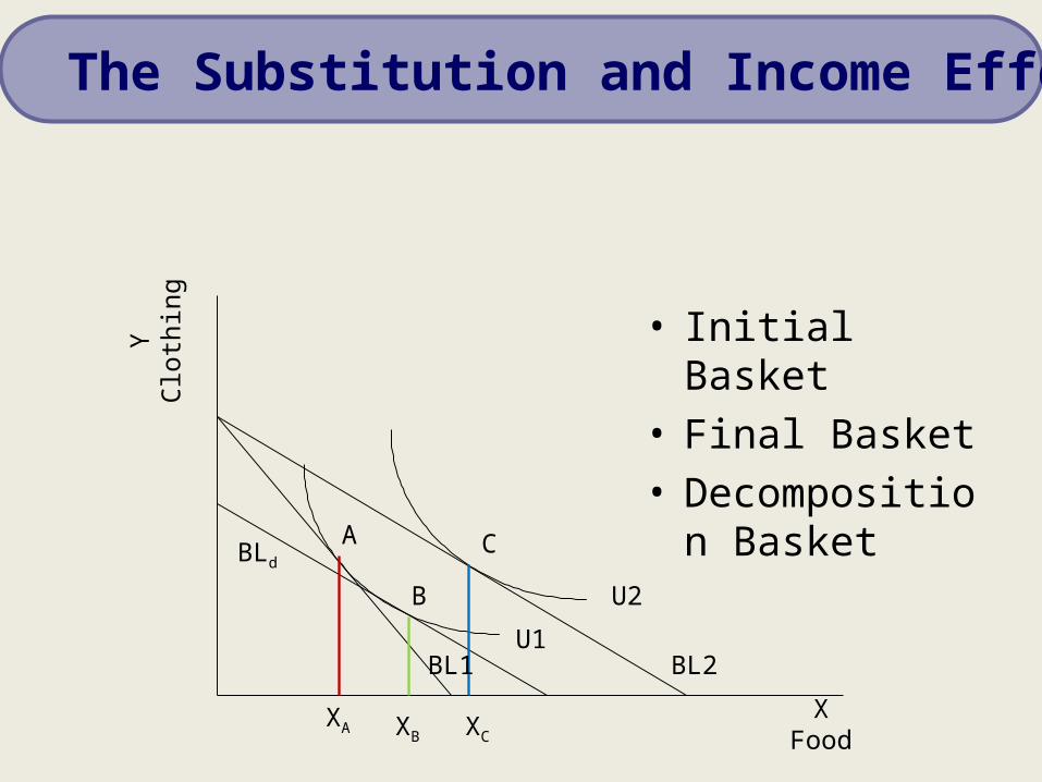
• Initial Basket• Final Basket• Decomposition

Basket

The Substitution and Income Effects

22Chapter Five


YC

loth

ing

XFood

A C

B

XA XCXB

BL1 BL2

BLd

U1

U2

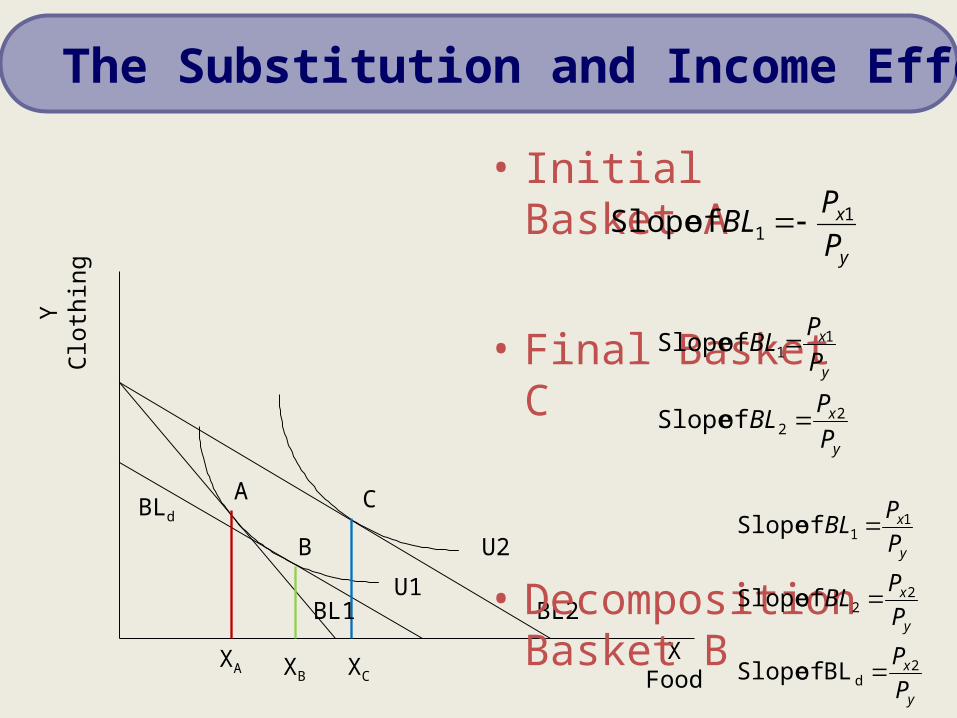
• Initial Basket A

• Final Basket C

• Decomposition Basket B

y

x

P

PBL 1

1 of Slope

y

x

y

x

P

PBL

P

PBL

22

11

of Slope

of Slope

y

x

y

x

y

x

P

P

P

PBL

P

PBL

2d

22

11

BL of Slope

of Slope

of Slope


24Chapter Five


25Chapter Five

Giffen Goods

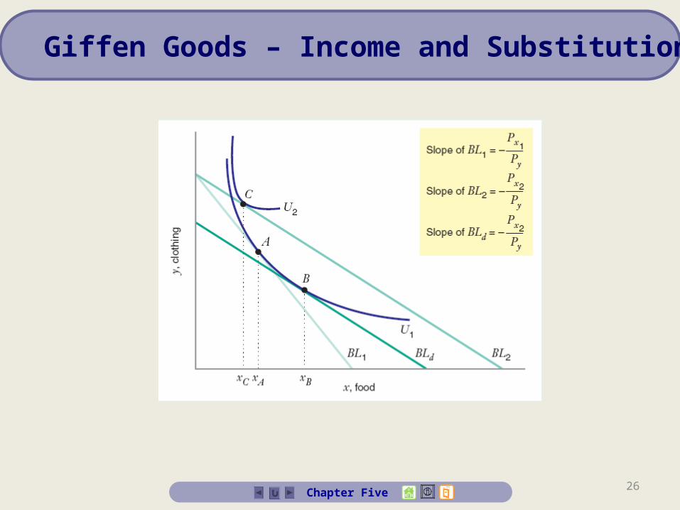
If a good is so inferior that the net effect of a price decrease of good x, all else constant, is a decrease in consumption of good x, good x is a Giffen good.

For Giffen goods, demand does not slope down.

When might an income effect be large enough to offset the substitution effect? The good would have to represent a very large proportion of the budget.

26Chapter Five

Giffen Goods – Income and Substitution Effects

27Chapter Five

Example – Income and Substitution Effects

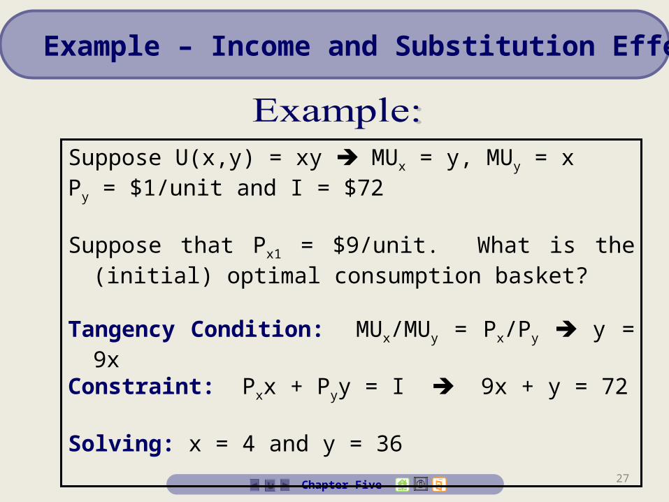
Suppose U(x,y) = xy MUx = y, MUy = xPy = $1/unit and I = $72

Suppose that Px1 = $9/unit. What is the (initial) optimal consumption basket?

Tangency Condition: MUx/MUy = Px/Py y = 9xConstraint: Pxx + Pyy = I 9x + y = 72

Solving: x = 4 and y = 36

28Chapter Five


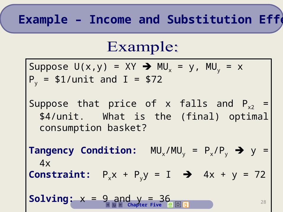
Suppose U(x,y) = XY MUx = y, MUy = xPy = $1/unit and I = $72

Suppose that price of x falls and Px2 = $4/unit. What is the (final) optimal consumption basket?

Tangency Condition: MUx/MUy = Px/Py y = 4xConstraint: Pxx + Pyy = I 4x + y = 72

Solving: x = 9 and y = 36

29Chapter Five


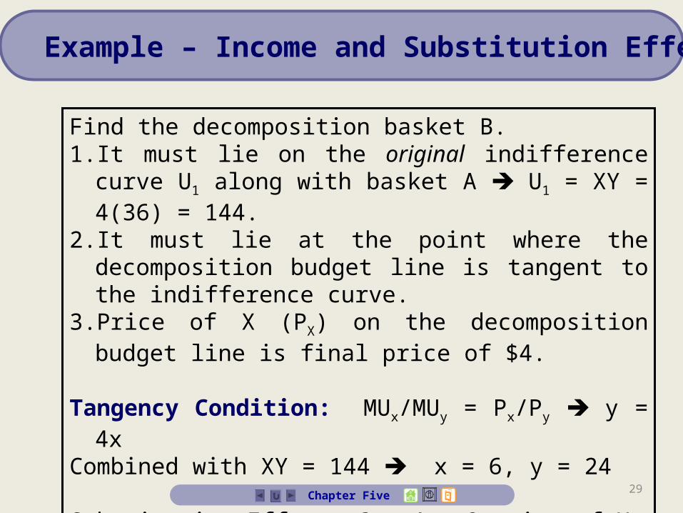
Find the decomposition basket B.1. It must lie on the original indifference curve U1 along with

basket A U1 = XY = 4(36) = 144.2. It must lie at the point where the decomposition budget

line is tangent to the indifference curve.3. Price of X (PX) on the decomposition budget line is final

price of $4.

Tangency Condition: MUx/MUy = Px/Py y = 4xCombined with XY = 144 x = 6, y = 24

Substitution Effect: 6 – 4 = 2 units of XIncome Effect: 9 – 6 = 3 units of X

30Chapter Five

Consumer Surplus

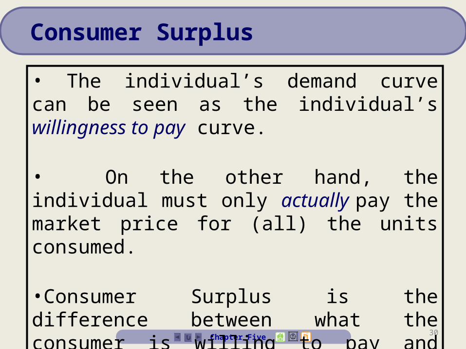
• The individual’s demand curve can be seen as the individual’s willingness to pay curve.

• On the other hand, the individual must only actually pay the market price for (all) the units consumed.

•Consumer Surplus is the difference between what the consumer is willing to pay and what the consumer actually pays.

31Chapter Five

Consumer Surplus

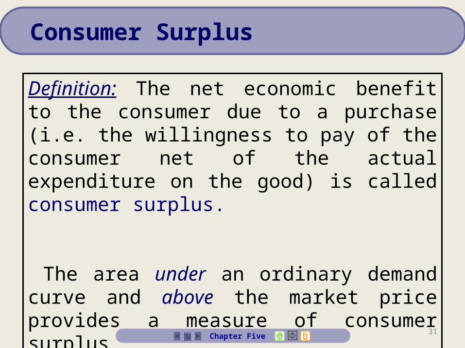
Definition: The net economic benefit to the consumer due to a purchase (i.e. the willingness to pay of the consumer net of the actual expenditure on the good) is called consumer surplus.

The area under an ordinary demand curve and above the market price provides a measure of consumer surplus

32Chapter Five

Consumer Surplus

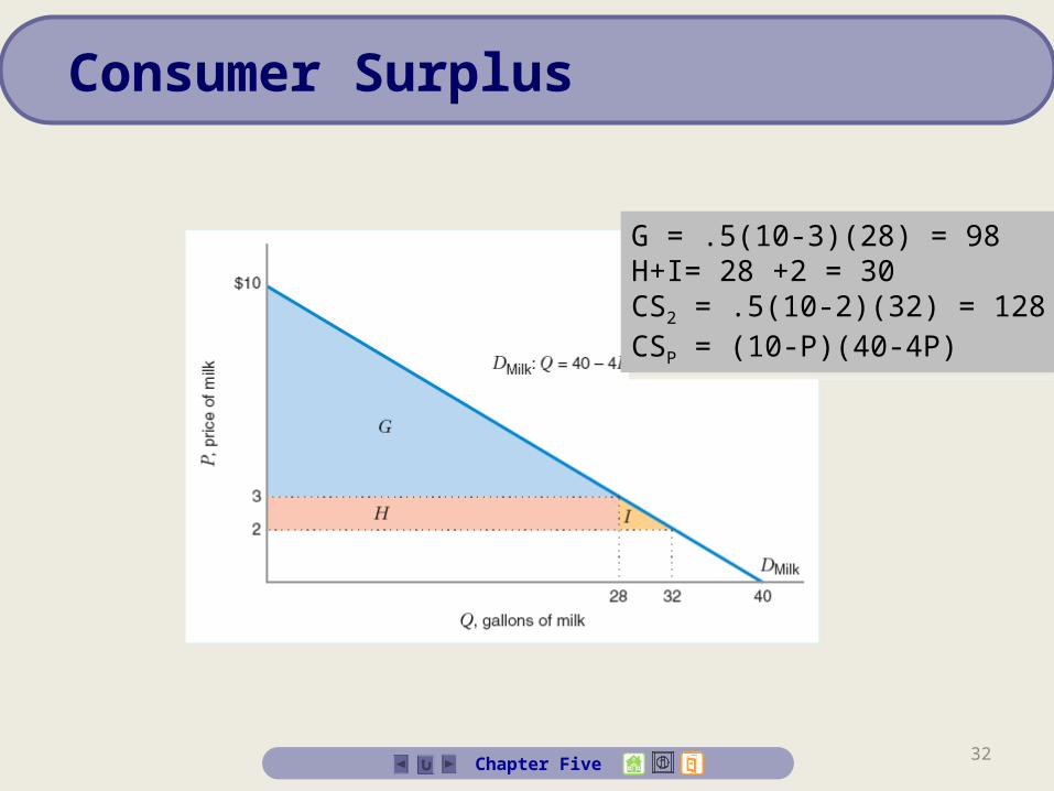
G = .5(10-3)(28) = 98H+I= 28 +2 = 30CS2 = .5(10-2)(32) = 128CSP = (10-P)(40-4P)

G = .5(10-3)(28) = 98H+I= 28 +2 = 30CS2 = .5(10-2)(32) = 128CSP = (10-P)(40-4P)

33Chapter Five

Market Demand

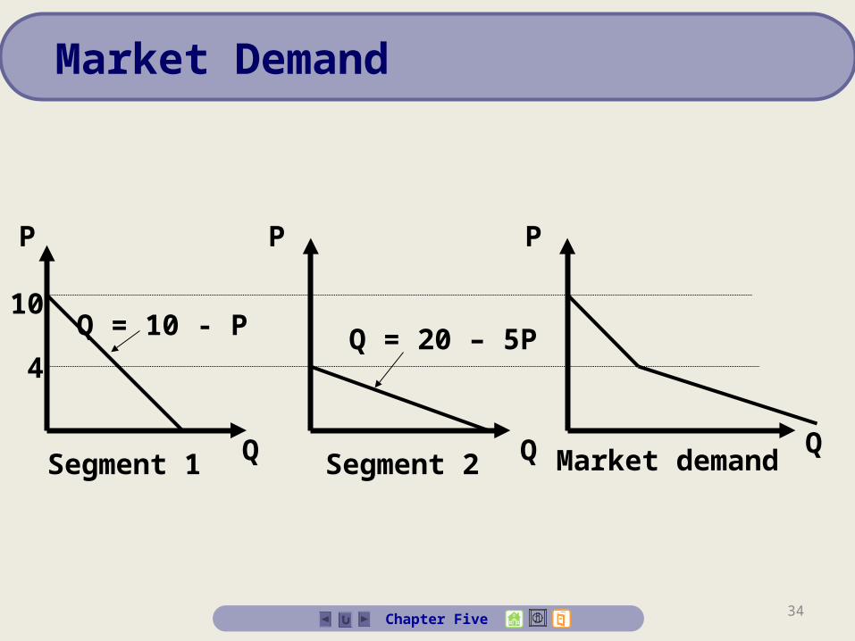
The market demand function is the horizontal sum of the individual (or segment) demands. In other words, market demand is obtained by adding the quantities demanded by the individuals (or segments) at each price and plotting this total quantity for all possible prices.

The market demand function is the horizontal sum of the individual (or segment) demands. In other words, market demand is obtained by adding the quantities demanded by the individuals (or segments) at each price and plotting this total quantity for all possible prices.

34

Q = 10 - P

Segment 1

Q = 20 – 5P

Segment 2 Market demand

4

10

Q Q Q

P P P

Chapter Five

Market Demand

• If one consumer's demand for a good changes with the number of other consumers who buy the good, there are network externalities.

Network Externalities

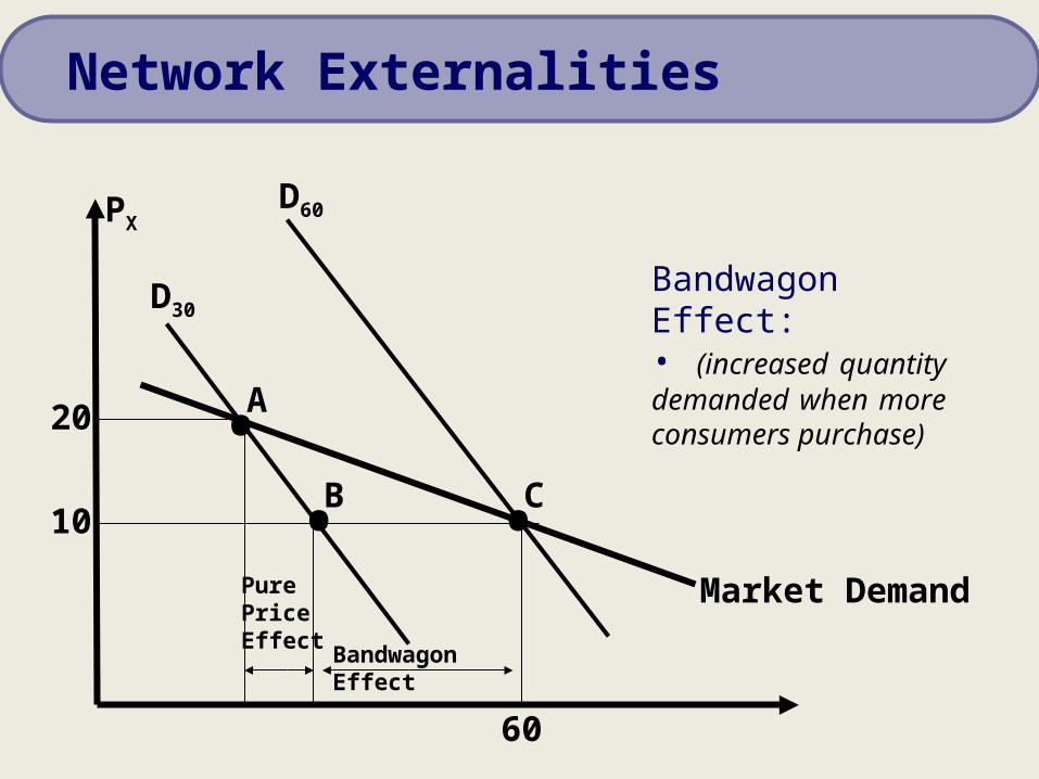
• Bandwagon effect: A positive network externality that refers to the increase in each consumer’s demand for a good as more consumers buy the good


PX

D30

D60

Market Demand

•• •

A

B C

20

10

60

PurePriceEffect

Bandwagon Effect

Bandwagon Effect:• (increased quantity demanded when more consumers purchase)


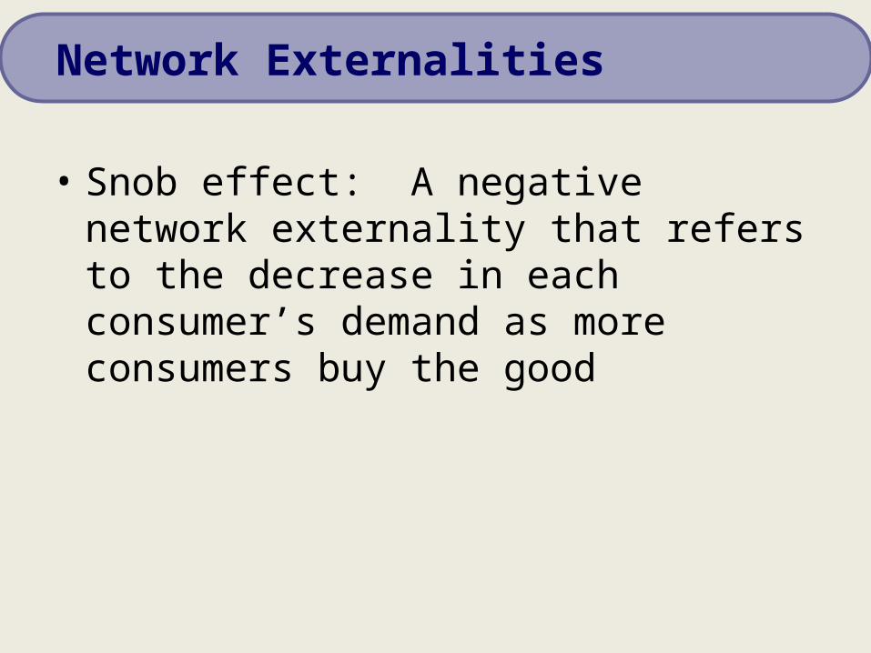
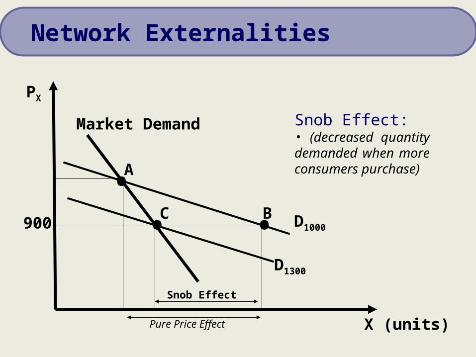
• Snob effect: A negative network externality that refers to the decrease in each consumer’s demand as more consumers buy the good


X (units)

PX

Market Demand

••

A

C900 D1000

D1300

•B

Pure Price Effect

Snob Effect

Snob Effect:• (decreased quantity demanded when more consumers purchase)


• Divide the day into two parts: Work hours and leisure (non work) hours.

• Earns income during work hours and uses the income to pay for activities he enjoys in his leisure time.

Labor-Leisure Trade-off

• Total Daily income:• w(24-L)

where w is the hourly wage rateL is the leisure hours24 is the 24 hours in a day

Defining Labor Supply

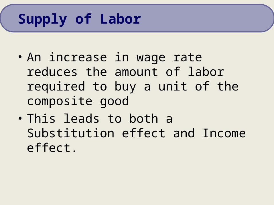
• An increase in wage rate reduces the amount of labor required to buy a unit of the composite good

• This leads to both a Substitution effect and Income effect.

Supply of Labor

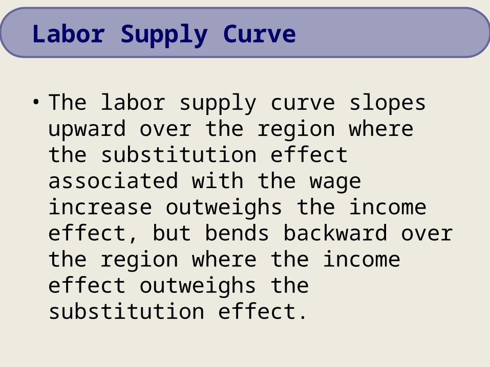
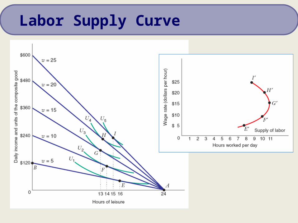
• The labor supply curve slopes upward over the region where the substitution effect associated with the wage increase outweighs the income effect, but bends backward over the region where the income effect outweighs the substitution effect.

Labor Supply Curve

Labor Supply Curve

Documents

The Theory Of Demand