Embed Size (px)
Citation preview
PhD THESIS
presented in order to obtain the degree of:
Docteur de l'Ecole Nationale Sup�erieure
des T�el�ecommunications
Speciality : Signal and Images
Mobile Localization in a GSM Network
Localisation d'un mobile dans un r�eseau GSM
Hassan El Nahas El Homsi
Defended on June 29, 1999, before the committee
composed of:
Bj�orn Ottersten Chairman
Jean-Jacques Fuchs Referees
Eric Moulines
Pierre Humblet Examiners
Philippe Loubaton
Dirk Slock
Jean-Louis Dornstetter Guests
Andr�e Terrom
Acknowledgments
First of all, I would like to thank Pierre Humblet, my thesis supervisor for his
continuous help and for motivating me.
I wish to thank Professor Bj�orn Ottersten from KTH for welcoming me in
his department in Stockholm. The two weeks of discussions I had with him and
his students were very fruitful. I wish also to thank him for accepting to be an
examiner of my thesis.
I equally thank Professor Eric Moulines for the several discussions I have had
with him during the thesis and for accepting to be an examiner of my thesis.
I also thank Professor Jean-Jacques Fuchs for accepting to be an examiner of
my thesis and for his detailed reading of the manuscript and his positive feedback.
I also wish to thank Professor Dirk Slock and Philippe Loubaton for accepting
to be on the Jury and for their general interest in my work.
I would like to thank all the people who surrounded me during the thesis
in Nortel Networks. A special thank is for Alexandre with whom I have had a
lot of discussions, his interest in my work is deeply appreciated. Many thanks
to Sophie, Anne, Sarah, Bastien, and Moussa who accepted to check my poor
english.
This paragraph would be of course incomplete if I didn't mention Jean-Louis
Dornstetter, Nidham Ben Rached, and Pierre Eisenmann who accepted me in the
R&D department in Nortel Networks. I also wish to thank Bouygues Telecom
for the �nancial support of this work.
I �nally want to express my deep gratitude to my parents for their constant
love and encouragement and for all they have sacri�ced for the success of their
children. It is to them that I dedicate this thesis.
i

ii
Abstract
The localization of a subscriber in a radio cellular network has attracted con-
siderable interest since the American Federal Communication Committee (FCC)
mandated all operators in the United States to localize their subscribers within
125 meters in 67 per cent of the cases by October 2001. This concerns essentially
emergency calls (E 911 calls). In addition to that, the localization technology has
several attractive applications such as navigation, home zone billing, fraud detec-
tion, and frequency planning enhancement. The North American standardization
committee has worked hard towards solving this issue for the various cellular stan-
dards. Many proposals have been presented by manufacturers. Their work shows
that the natural solution for the GSM standard should be based on the time of
arrival technology.
The main obstacle in time of arrival estimation is multipath. The goal is to
be able to estimate the time delay of the �rst path. A class of estimators based
on the extraction of the signal or the noise subspace is introduced. These estima-
tors o�er almost the same performances as the maximum likelihood with lower
complexities. An extension of these algorithms under model errors is introduced.
With at least three time of arrival measurements corresponding to three dif-
ferent base stations, it is possible to locate the handset under some conditions
on network synchronization. The maximum likelihood estimator leads to a non
linear maximization problem known as hyperbolic trilateration. Suboptimal algo-
rithms are presented o�ering good results at high signal-to-noise ratios. Complete
simulations are conducted in several typical environments such as urban or rural
areas incorporating synchronization errors. They show that a root mean square
error lower than one hundred meters is achievable in most cases.
iii

iv
R�esum�e
La localisation de mobiles dans un r�eseau radio cellulaire a re�cu un int�eret con-
sid�erable depuis que le comit�e f�ed�eral am�ericain de communication a demand�e
aux op�erateurs nord-am�ericains de localiser leurs abonn�es avec une pr�ecision de
125 m�etres dans 67 pour cent des cas. Ceci concerne essentiellement les appels
d'urgence. Outre les appels d'urgence, il existe d'autres applications comme la
navigation, la gestion de la taxation, la d�etection de fraudes et la plani�cation
cellulaire. Les travaux conduits par les comit�es am�ericains de normalisation ont
privil�egi�e les solutions bas�ees sur l'estimation du temps d'arriv�ee.
L'obstacle principal �a l'estimation du temps d'arriv�ee est le trajet multi-
ple. Il faut pouvoir estimer le retard temporel du premier trajet. Une classe
d'estimateurs bas�ee sur l'extraction des sous-espaces signal ou bruit est intro-
duite. Ces estimateurs o�rent quasiment les meme performances que l'estimateur
du maximum de vraisemblance tout en ayant une complexit�e moindre. Une ex-
tension de ces estimateurs en pr�esence d'erreurs de mod�ele est pr�esent�ee.
Avec un minimumde trois mesures de temps d'arriv�ee relatives �a trois di��erentes
stations de base, il est possible de localiser le mobile sous certaines conditions
de synchronisation du r�eseau. L'estimateur du maximum de vraisemblance con-
duit alors �a un probl�eme de maximisation non lin�eaire connu sous le nom de
triangulation hyperbolique. Des algorithmes sous-optimaux sont pr�esent�es mon-
trant d'excellents r�esultats lorsque le rapport signal sur bruit est su�samment
�elev�e. Des simulations exhaustives sont pr�esent�ees dans di��erents environnements
typiques comme les zones urbaines ou rurales en incluant des erreurs de synchro-
nisation. Elles montrent qu'une erreur quadratique moyenne inf�erieure �a cent
m�etres est possible dans la plupart des cas.
v

vi
Contents
Acknowledgements i
Abstract iii
R�esum�e v
1 Introduction 1
1.1 Locating a handset . . . . . . . . . . . . . . . . . . . . . . . . . . 3
1.2 Dissertation overview . . . . . . . . . . . . . . . . . . . . . . . . . 3
1.3 Contributions . . . . . . . . . . . . . . . . . . . . . . . . . . . . . 4
2 Wireless communications 7
2.1 Radio propagation model . . . . . . . . . . . . . . . . . . . . . . . 7
2.1.1 Path loss . . . . . . . . . . . . . . . . . . . . . . . . . . . . 7
2.1.2 Slow and fast fading, coherence time . . . . . . . . . . . . 8
2.1.3 Multipath and delay spread . . . . . . . . . . . . . . . . . 8
2.1.4 Interferences . . . . . . . . . . . . . . . . . . . . . . . . . . 9
2.1.5 Doppler spread . . . . . . . . . . . . . . . . . . . . . . . . 10
2.2 Protection techniques . . . . . . . . . . . . . . . . . . . . . . . . . 10
2.3 GSM system overview . . . . . . . . . . . . . . . . . . . . . . . . 11
2.3.1 The duplex physical channel . . . . . . . . . . . . . . . . . 11
2.3.2 Logical channels . . . . . . . . . . . . . . . . . . . . . . . . 13
2.3.3 Location Area Code (LAC) . . . . . . . . . . . . . . . . . 14
2.3.4 Handover . . . . . . . . . . . . . . . . . . . . . . . . . . . 15
2.3.5 The BSIC . . . . . . . . . . . . . . . . . . . . . . . . . . . 15
2.3.6 The GMSK modulation . . . . . . . . . . . . . . . . . . . 15
2.4 Channel equalization . . . . . . . . . . . . . . . . . . . . . . . . . 18
3 Technologies for location 23
3.1 Distance estimation from signal strength . . . . . . . . . . . . . . 23
3.2 Pattern matching based on training data . . . . . . . . . . . . . . 24
3.3 Angle of Arrival (AoA) estimation . . . . . . . . . . . . . . . . . . 24
3.4 Time of Arrival (ToA) estimation . . . . . . . . . . . . . . . . . . 25
vii
3.5 Hybrid methods - Joint Angle and Delay Estimation (JADE) . . . 26
3.6 Conclusion . . . . . . . . . . . . . . . . . . . . . . . . . . . . . . . 26
4 Time of arrival estimation 29
4.1 Notations and assumptions . . . . . . . . . . . . . . . . . . . . . . 29
4.2 Temporal approach . . . . . . . . . . . . . . . . . . . . . . . . . . 33
4.2.1 The Deterministic Maximum Likelihood (DML) . . . . . . 33
4.2.2 The Stochastic Maximum Likelihood (SML) . . . . . . . . 34
4.2.3 Channel impulse response estimation . . . . . . . . . . . . 35
4.2.4 Cramer-Rao Bound (CRB) . . . . . . . . . . . . . . . . . . 37
4.2.5 Some well-known estimators . . . . . . . . . . . . . . . . . 38
4.3 Frequency approach . . . . . . . . . . . . . . . . . . . . . . . . . . 40
4.3.1 Formulation . . . . . . . . . . . . . . . . . . . . . . . . . . 40
4.3.2 Some well-known estimators . . . . . . . . . . . . . . . . . 43
4.3.3 Forward-Backward averaging . . . . . . . . . . . . . . . . . 46
4.4 Simulations . . . . . . . . . . . . . . . . . . . . . . . . . . . . . . 46
4.5 Extension to an unknown modulation pulse . . . . . . . . . . . . 49
4.5.1 Iterative approach . . . . . . . . . . . . . . . . . . . . . . 53
4.5.2 A modi�ed ESPRIT algorithm . . . . . . . . . . . . . . . . 54
4.5.3 The DToA special case . . . . . . . . . . . . . . . . . . . . 55
4.5.4 Simulations . . . . . . . . . . . . . . . . . . . . . . . . . . 56
4.6 On complexity . . . . . . . . . . . . . . . . . . . . . . . . . . . . . 57
5 Hyperbolic trilateration 59
5.1 Problem statement . . . . . . . . . . . . . . . . . . . . . . . . . . 59
5.2 Cramer-Rao bound . . . . . . . . . . . . . . . . . . . . . . . . . . 62
5.3 Algorithms for hyperbolic trilateration . . . . . . . . . . . . . . . 63
5.3.1 Taylor expansion (scoring method) . . . . . . . . . . . . . 63
5.3.2 Least squares . . . . . . . . . . . . . . . . . . . . . . . . . 64
5.4 Simulations and results . . . . . . . . . . . . . . . . . . . . . . . . 66
6 On network synchronization 71
6.1 The pseudo-synchronization problem . . . . . . . . . . . . . . . . 72
6.2 Absolute synchronization . . . . . . . . . . . . . . . . . . . . . . . 75
7 Global simulations and �nal results 79
7.1 Channel impulse response model . . . . . . . . . . . . . . . . . . . 79
7.2 Environment pro�les . . . . . . . . . . . . . . . . . . . . . . . . . 81
7.3 Time of Arrival simulations . . . . . . . . . . . . . . . . . . . . . 82
7.3.1 Assumptions . . . . . . . . . . . . . . . . . . . . . . . . . . 82
7.3.2 Simulations . . . . . . . . . . . . . . . . . . . . . . . . . . 83
7.4 Location simulations . . . . . . . . . . . . . . . . . . . . . . . . . 89
7.4.1 Assumptions . . . . . . . . . . . . . . . . . . . . . . . . . . 90
viii
7.4.2 Results of simulations . . . . . . . . . . . . . . . . . . . . 90
8 Conclusion and further research 101
9 R�esum�e d�etaill�e en fran�cais 103
9.1 Introduction . . . . . . . . . . . . . . . . . . . . . . . . . . . . . . 103
9.2 Communications sans �l . . . . . . . . . . . . . . . . . . . . . . . 104
9.2.1 Mod�ele de propagation radio . . . . . . . . . . . . . . . . . 104
9.2.2 Aper�cu de la norme GSM . . . . . . . . . . . . . . . . . . 105
9.2.3 Egalisation . . . . . . . . . . . . . . . . . . . . . . . . . . 106
9.3 Technologies pour la localisation . . . . . . . . . . . . . . . . . . . 108
9.4 Estimation du temps d'arriv�ee . . . . . . . . . . . . . . . . . . . . 109
9.4.1 Notations et hypoth�eses . . . . . . . . . . . . . . . . . . . 109
9.4.2 Approche temporelle . . . . . . . . . . . . . . . . . . . . . 109
9.4.3 Approche fr�equentielle . . . . . . . . . . . . . . . . . . . . 111
9.4.4 Extension au cas d'une modulation inconnue . . . . . . . . 114
9.4.5 Simulations . . . . . . . . . . . . . . . . . . . . . . . . . . 116
9.5 Triangulation hyperbolique . . . . . . . . . . . . . . . . . . . . . . 118
9.6 Synchronisation du r�eseau . . . . . . . . . . . . . . . . . . . . . . 122
9.7 Simulations globales . . . . . . . . . . . . . . . . . . . . . . . . . 124
9.7.1 Mod�ele de canal . . . . . . . . . . . . . . . . . . . . . . . . 125
9.7.2 Estimation du temps d'arriv�ee . . . . . . . . . . . . . . . . 126
9.7.3 Estimation de la position . . . . . . . . . . . . . . . . . . . 128
9.8 Conclusions et directions futures . . . . . . . . . . . . . . . . . . . 130
Appendices 133
A GMSK pulse 133
B Proof for the variance formula 137
C Derivation of the Cramer-Rao bound 139
D Mathematical notations 141
E Abbreviations 143
Bibliography 145
ix

x
List of Figures
1.1 PLMN architecture . . . . . . . . . . . . . . . . . . . . . . . . . . . 2
2.1 Normal burst format . . . . . . . . . . . . . . . . . . . . . . . . . . 12
2.2 Access burst format . . . . . . . . . . . . . . . . . . . . . . . . . . 12
2.3 Synchronization burst format . . . . . . . . . . . . . . . . . . . . . 12
2.4 GMSK main pulse . . . . . . . . . . . . . . . . . . . . . . . . . . . 17
4.1 The GMSK main pulse and its �ltered versions at 0:8=T and 1=T . . . 47
4.2 Temporal MUSIC and matched �ltering (cross-correlation) at 10 dB, 5
independent trials are run: the matched �lter is unable to resolve two
delays equally powered spaced by one bit period. . . . . . . . . . . . 48
4.3 Algorithm performance with respect to the SNR, L = 100 synch. bursts
are used, �� = T , and � = 0: MUSIC and Root WSF are e�cient. . . 49
4.4 Algorithm performance with respect to the SNR, L = 100 synch. bursts
are used, �� = T , � = 0:99: only Root WSF is e�cient. . . . . . . . . 49
4.5 Algorithm performance with respect to the number of bursts at 8 dB,
�� = T , � = 0. . . . . . . . . . . . . . . . . . . . . . . . . . . . . . 50
4.6 Algorithm performance with respect to the delays separation at 8 dB,
L = 100 synch. bursts used, � = 0. . . . . . . . . . . . . . . . . . . . 50
4.7 The E�ect of forward-backward averaging: �� = 1T, � = 0. (a) with
ESPRIT using 10 synch bursts, (b) with ESPRIT using 100 synch.
bursts, (c) with Root WSF using 50 bursts. Forward-Backward averag-
ing is useful for suboptimal methods especially if few number of bursts
are available. However, it should not be used for optimal methods such
as Root WSF, Figure (c) shows no improvement in performance when
using forward-backward averaging. . . . . . . . . . . . . . . . . . . . 51
4.8 Temporal MUSIC and matched �ltering (cross-correlation): 5 indepen-
dent trials are run at 10 dB and using 100 synch. bursts showing that
a bias appears when a wrong pulse is assumed. The wrong pulse here
is the GMSK main pulse �ltered at 0.8/T. . . . . . . . . . . . . . . . 52
4.9 ESPRIT with and without the knowledge of the pulse, �� = T , L = 200
synch. bursts are used. . . . . . . . . . . . . . . . . . . . . . . . . . 56
xi
4.10 Algorithm performance with an unknown pulse, �� = T , � = 0, '*'
refers to the non-iterative ESPRIT-like's approach and 'o' refers to the
iterative approach performed using Root WSF. . . . . . . . . . . . . 57
5.1 Network architecture: 'o' represents a base station and the dots refer
to several handset positions. . . . . . . . . . . . . . . . . . . . . . . 67
5.2 CRB with and without the knowledge of the timing advance, �ve base
stations are involved in the trilateration. . . . . . . . . . . . . . . . . 68
5.3 Algorithms simulations . . . . . . . . . . . . . . . . . . . . . . . . . 68
5.4 Chan's approach vs. the CRB. . . . . . . . . . . . . . . . . . . . . . 69
6.1 The pseudo-synchronization problem. There are three cycles in this
network, the sum of the RTDs on each of them is by de�nition null. All
base stations are connected to the network. . . . . . . . . . . . . . . 73
6.2 �(�) variations according to the number of neighbors per base station,
� = 0:5. . . . . . . . . . . . . . . . . . . . . . . . . . . . . . . . . . 78
7.1 Nakagami Distribution . . . . . . . . . . . . . . . . . . . . . . . . . 81
7.2 Urban pro�le example, 20 consecutive bursts are generated: (a) at 2
km/h, (b) at 50 km/h. At high speed, the fading is less correlated in
time. There is no line of sight path and a bias in the ToA estimation
is unavoidable. . . . . . . . . . . . . . . . . . . . . . . . . . . . . . 84
7.3 Rural pro�le example, 20 consecutive bursts are generated: (a) at 3
km/h, (b) at 100 km/h. A strong line of sight path is always present. . 85
7.4 Eigenvalues behaviour in urban environment according to: (a) the dis-
tance, (b) mobile speed. . . . . . . . . . . . . . . . . . . . . . . . . 86
7.5 Eigenvalues behaviour in rural environment according to: (a) the dis-
tance, (b) mobile speed. . . . . . . . . . . . . . . . . . . . . . . . . 87
7.6 ToA estimation error histogram at 3 km/h and 10 dB using 20 synch.
bursts for: (a) rural environment at 10 km, (b) urban environment at
1 km. . . . . . . . . . . . . . . . . . . . . . . . . . . . . . . . . . . 89
7.7 ToA estimation in the urban environment: (a) for di�erent mobile
speeds, (b) for di�erent number of bursts, (c) for di�erent distances
MS-BS, (d) for di�erent maximum signal subspace dimensions. . . . . 91
7.8 ToA estimation in the suburban environment: (a) for di�erent mobile
speeds, (b) for di�erent number of bursts, (c) for di�erent distances
MS-BS, (d) for di�erent maximum signal subspace dimensions. . . . . 92
7.9 ToA estimation in the rural environment: (a) for di�erent mobile speeds,
(b) for di�erent number of bursts, (c) for di�erent distances MS-BS, (d)
for di�erent maximum signal subspace dimensions. . . . . . . . . . . 93
7.10 Network model with a reuse pattern of 7 cells. . . . . . . . . . . . . . 94
7.11 Network model, urban pro�le, all mobiles are generated in the middle
of the network to avoid border e�ects. . . . . . . . . . . . . . . . . . 94
xii
7.12 C/I CDF for the BCCH channel for the serving cell and the nearest
three base stations: urban pro�les are interference limited while rural
and suburban pro�les are noise limited. . . . . . . . . . . . . . . . . 95
7.13 Location estimation in the urban environment with synchronization
errors: (a) at 3 km/h, (b) at 50 km/h. . . . . . . . . . . . . . . . . . 97
7.14 Location estimation in the urban indoor environment with syn-
chronization errors: 3 km/h. . . . . . . . . . . . . . . . . . . . . . 98
7.15 Location estimation in the rural environment with synchronization er-
rors: (a) at 3 km/h, (b) at 100 km/h. . . . . . . . . . . . . . . . . . 99
7.16 Location estimation in the suburban environment with synchronization
errors: (a) at 3 km/h, (b) at 50 km/h. . . . . . . . . . . . . . . . . . 100
9.1 Impulsion GMSK principale . . . . . . . . . . . . . . . . . . . . . . 107
9.2 Performances des algorithmes en fonction du rapport signal sur bruit,
L = 100 bursts de synchronisation sont utilis�es, �� = 1T et � = 0. . . 117
9.3 Performances des algorithmes en fonction du rapport signal sur bruit,
L = 100 bursts de synchronisation sont utilis�es, �� = 1T et � = 0:99. . 117
9.4 ESPRIT et ESPRIT modi��e, L = 200 bursts de synchronisation sont
utilis�es. . . . . . . . . . . . . . . . . . . . . . . . . . . . . . . . . . 118
9.5 Mod�ele : 'o' repr�esente une station de base et les points di��erentes
positions de mobiles. . . . . . . . . . . . . . . . . . . . . . . . . . . 121
9.6 R�esultats de simulation . . . . . . . . . . . . . . . . . . . . . . . . . 122
9.7 Le probl�eme de la pseudo-synchronisation : il y a trois cycles dans ce
r�eseau, la somme des RTD sur chacun d'eux est par d�e�nition nulle. . 123
9.8 CDF pour le pro�l urbain : (a) �a 3 km/h, (b) �a 50 km/h. . . . . . . . 131
A.1 The modulation function in the GMSK. . . . . . . . . . . . . . . . 134
A.2 GMSK main and secondary pulses. . . . . . . . . . . . . . . . . . 135
A.3 GMSK spectrum. . . . . . . . . . . . . . . . . . . . . . . . . . . . 135
xiii

xiv
List of Tables
3.1 Summary of the di�erent technologies . . . . . . . . . . . . . . . . . 27
7.1 Time of arrival simulations assumptions according to each pro�le. . . . 83
7.2 RMS error (in meters) for the best 90% results of ToA simulation results
at 10 dB and using 20 synch. bursts. . . . . . . . . . . . . . . . . . . 90
7.3 Location simulations assumptions according to each pro�le. . . . . . . 91
7.4 Location simulations results with three, four, and �ve base stations.
Network perfectly synchronized. . . . . . . . . . . . . . . . . . . . . 96
7.5 Location simulations results with three, four, and �ve base stations.
Synchronization errors are included. . . . . . . . . . . . . . . . . . . 96
9.1 Param�etres de simulations du temps d'arriv�ee pour les di��erents pro�ls. 127
9.2 Racine de l'erreur quadratique moyenne (en m�etres) pour les 90% meilleurs
r�esultats en utilisant 20 bursts de synchronisation. . . . . . . . . . . . 128
9.3 Param�etres des simulations de la localisation pour les di��erents pro�ls. 129
9.4 R�esultats des simulations avec trois, quatre et cinq stations de base.
Synchronisation parfaite. . . . . . . . . . . . . . . . . . . . . . . . . 130
9.5 R�esultats des simulations avec trois, quatre et cinq stations de base.
Les erreurs de synchronisation sont incluses. . . . . . . . . . . . . . . 130
xv

xvi
Chapter 1
Introduction
Since the cellular concept was introduced in the 60's, wireless technologies have
known a fast development. The main enhancement was the introduction of digital
communications instead of the classical analog communications. This is mainly
due to Shannon's work on information theory. Many digital standards exist nowa-
days. They represent the second generation standards, mainly DAMPS, GSM,
and IS-95 CDMA.
The digital technology has permitted a rapid increase in the performances of
cellular systems. We can distinguish now between two kinds of standards: the
�rst is based on Time Division Multiple Access (TDMA) and the second is based
on the Code Division Multiple Access (CDMA). The GSM system is the most
widely used system nowadays and it is most likely that it has several years left
before the third generation emerges.
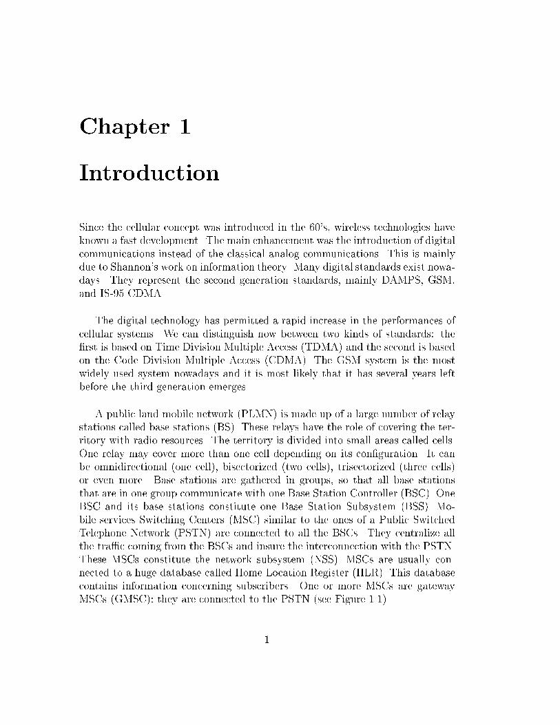
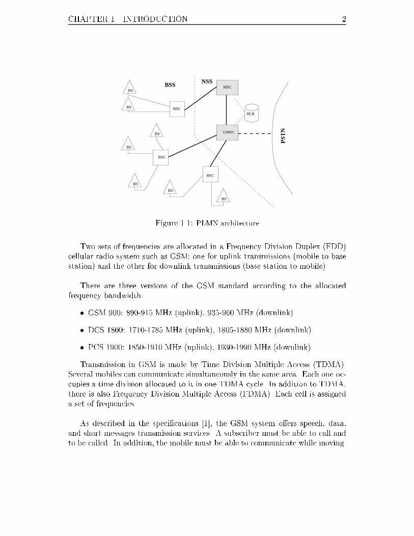
A public land mobile network (PLMN) is made up of a large number of relay
stations called base stations (BS). These relays have the role of covering the ter-
ritory with radio resources. The territory is divided into small areas called cells.
One relay may cover more than one cell depending on its con�guration. It can
be omnidirectional (one cell), bisectorized (two cells), trisectorized (three cells)
or even more. Base stations are gathered in groups, so that all base stations
that are in one group communicate with one Base Station Controller (BSC). One
BSC and its base stations constitute one Base Station Subsystem (BSS). Mo-
bile services Switching Centers (MSC) similar to the ones of a Public Switched
Telephone Network (PSTN) are connected to all the BSCs. They centralize all
the tra�c coming from the BSCs and insure the interconnection with the PSTN.
These MSCs constitute the network subsystem (NSS). MSCs are usually con-
nected to a huge database called Home Location Register (HLR). This database
contains information concerning subscribers. One or more MSCs are gateway
MSCs (GMSC): they are connected to the PSTN (see Figure 1.1).
1
CHAPTER 1. INTRODUCTION 2
HLR
GMSC
MSC
BSC
BSC
BSC
BS
BS
BS
BS
BS
BS
BS
PST
N
NSSBSS
Figure 1.1: PLMN architecture
Two sets of frequencies are allocated in a Frequency Division Duplex (FDD)
cellular radio system such as GSM: one for uplink transmissions (mobile to base
station) and the other for downlink transmissions (base station to mobile).
There are three versions of the GSM standard according to the allocated
frequency bandwidth:
� GSM 900: 890-915 MHz (uplink), 935-960 MHz (downlink).
� DCS 1800: 1710-1785 MHz (uplink), 1805-1880 MHz (downlink).
� PCS 1900: 1850-1910 MHz (uplink), 1930-1990 MHz (downlink).
Transmission in GSM is made by Time Division Multiple Access (TDMA).
Several mobiles can communicate simultaneously in the same area. Each one oc-
cupies a time division allocated to it in one TDMA cycle. In addition to TDMA,
there is also Frequency Division Multiple Access (FDMA). Each cell is assigned
a set of frequencies.
As described in the speci�cations [1], the GSM system o�ers speech, data,
and short messages transmission services. A subscriber must be able to call and
to be called. In addition, the mobile must be able to communicate while moving.
3 1.1. LOCATING A HANDSET
1.1 Locating a handset
In June 1996, the American Federal Communication Committee (FCC) requested
all North American mobile cellular networks to meet some requirements on the
location of emergency calls by October 2001. These operators must be able to
locate an emergency call made by one of their subscribers within 125 meters in
67 per cent of cases.
The localization technology has several additional applications. These appli-
cations are mainly accident reports, navigation, home zone billing, fraud detec-
tion, and statistical measurements (handover failure, tra�c location).
Locating a handset is often associated to GPS, which is a well-known satellite-
based technology for locating a compatible handset everywhere on the Earth in
three dimensions. However, this attractive system has several drawbacks. Al-
though it has a quite complete coverage of the Earth, it cannot work in general
in some di�cult environments such as urban environments or indoor environ-
ments since it requires the visibility of at least four satellites. It is possible to
o�er location services by using the already installed infra-structures of cellular
networks whenever the mobile handset is in a covered area. The accuracy of the
estimated position can be signi�cantly better than with GPS. The aim of this
dissertation is to show that it is possible to locate a mobile handset using the
network's own capability.
The location computation itself is done in a entity called Mobile Location
Center (MLC). This entity can be implemented in the mobile, in the network,
or even somewhere else. The Mobile Location Center (MLC) needs all collected
measurements performed at the handset or in the network and some other data
related to the network architecture. There exist many possible techniques to
locate a handset:
� Geometric approaches based on measurements of time of arrival, distance,
angle of arrival, or signal level strength.
� Pattern matching approaches based on the analysis of some control param-
eters by matching them on prediction maps previously computed.
Synchronization is also a topic related to location. It is fully required in all
methods based on time of arrival measurements.
1.2 Dissertation overview
This work addresses the problem of estimating a mobile handset position in a
GSM radio network using time of arrival estimation.
CHAPTER 1. INTRODUCTION 4
Chapter 2 is a description of the physical layer of the GSM standard. Di�erent
logical channels are described. The di�erent kinds of bursts used are presented
too. The GMSK modulation used in GSM is depicted; it is shown to be almost
linear though it is a phase modulation.
Chapter 3 discusses the di�erent ways of locating a handset. Time of arrival,
angle of arrival, signal strength, and pattern matching approaches are discussed.
The time of arrival approach will be retained as being acceptable in terms of
accuracy and complexity.
Chapter 4 discusses the problem of time of arrival estimation. The environ-
ment is assumed to exhibit discrete (specular) multipath components. No di�use
paths are present. The maximum likelihood estimator is used and shown to be
more accurate than the classical estimator known as the matched �lter (cross-
correlator). Two sets of algorithms are presented in the time and the frequency
domain. A link with array processing techniques is established. An extension to
the case of an unknown modulation pulse is discussed.
Chapter 5 is a study of the hyperbolic trilateration procedure that is used to
estimate the mobile position with at least three time of arrival measurements.
It is shown that the lack of knowledge of a time reference leads to a hyperbolic
trilateration made from di�erences of times of arrival so that the time reference
contribution disappears.
Chapter 6 is a brief discussion on the synchronization issue: the problems of
pseudo-synchronization and absolute synchronization are discussed separately.
Chapter 7 is the chapter of simulations. The channel model of the American
normalization committee is used in order to perform simulations of both the time
of arrival estimation and the hyperbolic trilateration on realistic environments.
Chapter 8 is a conclusion. It discusses also some possible future directions.
1.3 Contributions
This dissertation treats the important aspects of a cellular localization system:
� Basic principles: this localization system is based on time of arrival esti-
mation followed by a hyperbolic trilateration in a synchronized or pseudo-
synchronized network.

5 1.3. CONTRIBUTIONS
� Time of arrival estimation: an analogy with array processing is presented.
A rigorous development shows the possibility of substituting the signal
samples with the least squares estimate of the channel impulse response
(achieved by means of the training sequence) without any loss in perfor-
mances. Many algorithms are adapted to the particular problem of time of
arrival estimation. Extension to the case of unknown modulation pulse is
analyzed: an original ESPRIT-like algorithm is presented.
� Hyperbolic trilateration: Cramer-Rao computation with and without knowl-
edge of the timing advance. Several algorithms are simulated and compared.
The Taylor expansion algorithm shows ideal results at low signal-to-noise
ratios.
� Synchronization: description of a general algorithm for the estimation of
the di�erence of transmission times between base stations by exploiting
noisy measurements performed on the radio side of the network.
In addition to these theoretical studies, several contributions have been presented
to the American standardization committee T1P1.5 on the elaboration of a com-
mon channel model. Simulations have been conducted based on this model. A
standard has since been adopted.

CHAPTER 1. INTRODUCTION 6
Chapter 2
Wireless communications
In the following, we describe the problems caused by the radio propagation envi-
ronment and the techniques used for protecting communications. We describe the
GSM system as a typical radio cellular network and discuss its radio modulation
in details. We detail the equalization procedure or more precisely the channel
impulse response estimation when a given training sequence is available.
2.1 Radio propagation model
The radio interface is the most di�cult part in the cellular concept. This is mainly
due to the channel propagation characteristics that corrupt the communications.
For this purpose, a permanent signaling dialog exists between the mobile and the
network whether the mobile is in communication or not.
2.1.1 Path loss
As the radio signal propagates, its intensity decreases. Indeed, the signal energy
is distributed on a spherical front. In free space, the path loss is proportional to
d�2 where d refers to the distance of propagation between the transmitter and
the receiver. In typical environments such as urban or rural areas, there exist
many empirical models that compute the path loss according to some parameters
such as the distance or the height of the antenna. It is common to state that the
path loss is proportional to d�
10 where 2 [20; 40].
The Okumura-Hata formula [2] is perhaps the best known empirical formula
used to compute the received power:
Pr = Pt + ga � Lp � log(d) (2.1)
where Pt is the transmitted power, ga is the antenna gain in the signal di-
rection, Lp is the path loss at one km. This equation is expressed in dB. The
7
CHAPTER 2. WIRELESS COMMUNICATIONS 8
received power Pr represents a mean value, it is subject to variations around its
mean value due to slow fading.
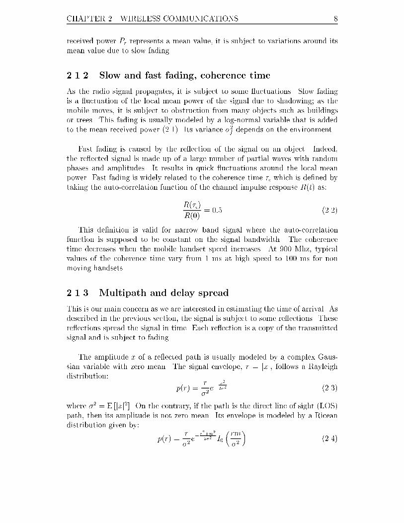
2.1.2 Slow and fast fading, coherence time
As the radio signal propagates, it is subject to some uctuations. Slow fading
is a uctuation of the local mean power of the signal due to shadowing; as the
mobile moves, it is subject to obstruction from many objects such as buildings
or trees. This fading is usually modeled by a log-normal variable that is added
to the mean received power (2.1). Its variance �2fdepends on the environment.
Fast fading is caused by the re ection of the signal on an object. Indeed,
the re ected signal is made up of a large number of partial waves with random
phases and amplitudes. It results in quick uctuations around the local mean
power. Fast fading is widely related to the coherence time �c which is de�ned by
taking the auto-correlation function of the channel impulse response R(t) as:
R(�c)
R(0)= 0:5 (2.2)
This de�nition is valid for narrow band signal where the auto-correlation
function is supposed to be constant on the signal bandwidth. The coherence
time decreases when the mobile handset speed increases. At 900 Mhz, typical
values of the coherence time vary from 1 ms at high speed to 100 ms for non
moving handsets.
2.1.3 Multipath and delay spread
This is our main concern as we are interested in estimating the time of arrival. As
described in the previous section, the signal is subject to some re ections. These
re ections spread the signal in time. Each re ection is a copy of the transmitted
signal and is subject to fading.
The amplitude x of a re ected path is usually modeled by a complex Gaus-
sian variable with zero mean. The signal envelope, r = jxj, follows a Rayleigh
distribution:
p(r) =r
�2e�
r2
2�2 (2.3)
where �2 = E [jxj2]. On the contrary, if the path is the direct line of sight (LOS)
path, then its amplitude is not zero mean. Its envelope is modeled by a Ricean
distribution given by:
p(r) =r
�2e�
r2+m
2
2�2 I0
�rm
�2
�(2.4)
9 2.1. RADIO PROPAGATION MODEL
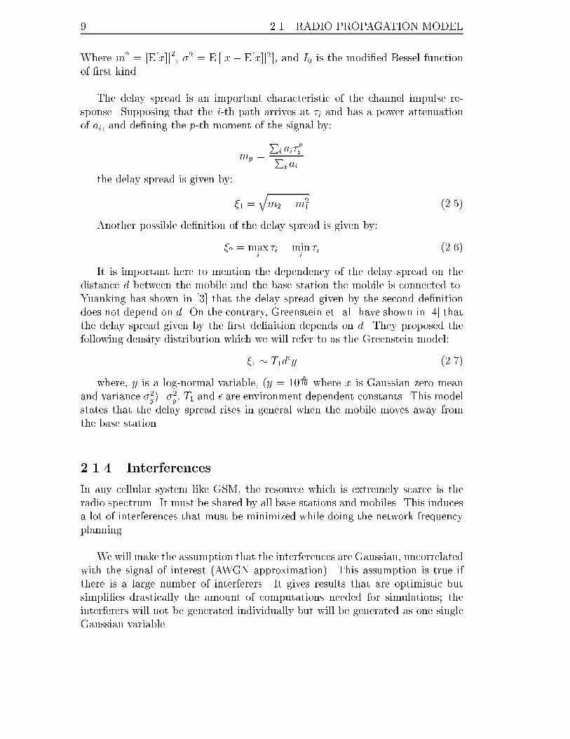
Where m2 = jE[x]j2, �2 = E [jx� E[x]j2], and I0 is the modi�ed Bessel function
of �rst kind.
The delay spread is an important characteristic of the channel impulse re-
sponse. Supposing that the i-th path arrives at �i and has a power attenuation
of ai, and de�ning the p-th moment of the signal by:
mp =
Pi ai�
p
iPi ai
the delay spread is given by:
�1 =qm2 �m2
1 (2.5)
Another possible de�nition of the delay spread is given by:
�2 = maxi�i �min
i�i (2.6)
It is important here to mention the dependency of the delay spread on the
distance d between the mobile and the base station the mobile is connected to.
Yuanking has shown in [3] that the delay spread given by the second de�nition
does not depend on d. On the contrary, Greenstein et. al. have shown in [4] that
the delay spread given by the �rst de�nition depends on d. They proposed the
following density distribution which we will refer to as the Greenstein model:
�1 � T1d�y (2.7)
where, y is a log-normal variable, (y = 10x
10 where x is Gaussian zero mean
and variance �2y). �2
y, T1 and � are environment dependent constants. This model
states that the delay spread rises in general when the mobile moves away from
the base station.
2.1.4 Interferences
In any cellular system like GSM, the resource which is extremely scarce is the
radio spectrum. It must be shared by all base stations and mobiles. This induces
a lot of interferences that must be minimized while doing the network frequency
planning.
We will make the assumption that the interferences are Gaussian, uncorrelated
with the signal of interest (AWGN approximation). This assumption is true if
there is a large number of interferers. It gives results that are optimistic but
simpli�es drastically the amount of computations needed for simulations; the
interferers will not be generated individually but will be generated as one single
Gaussian variable.
CHAPTER 2. WIRELESS COMMUNICATIONS 10
2.1.5 Doppler spread
As the mobile moves, the signal is subject to the Doppler e�ect that shifts it
in frequency. This shift becomes more and more important as speed increases.
The Doppler shift is given by v
�cos(�), where � is the angle between the signal
direction of arrival and the mobile direction. At 900 MHz, the maximum shift,
fd =v
�, is about one Hertz per km/h.
2.2 Protection techniques
� Channel coding and interleaving: channel coding is a powerful technique to
secure the transmitted bits against fading. It consists in adding redundant
information to the source data. The codes used in GSM are some convolu-
tional codes and one Fire code. Depending on the transmitted information,
some bits are protected more than others. Interleaving consists in shu�ing
the bits before putting them in bursts. The consequence is better protection
against block fading.
� Discontinuous transmission (DTX) consists in transmitting at a reduced
rate during a voice communication when nothing is said and silence remains.
In GSM, the reduced rate is about 12 % of the normal rate. The main
advantage of DTX is that it reduces the average interference and increases
the handset battery life.
� Power control: like DTX, power control is a technique that limits the av-
erage interference and saves the handset battery life. When the communi-
cation quality is good enough, it is worthless to transmit at a high signal
level. In this case, the mobile is requested to transmit at a lower level.
� Slow frequency hopping: Slow frequency hopping used in TDMA systems
consists in changing the frequency carrier at regular intervals. Since the
fading is frequency selective, the signals sent are independent even at low
speed. This property is sometimes called frequency diversity. Fast fre-
quency hopping, where the frequency changes at the modulation rate, is
not used in GSM.
� Space diversity: this technique is used nowadays for uplink receivers only,
but it could be used for downlink receivers in the near future. At the
reception end, the base station has several antennae. The base station thus
receives several copies of the same signal. The gain obtained from diversity
is proportional to the number of antennae. Usually, two antennae are used
providing a gain greater than 3 dB.
� Training sequences: this technique consists in sending a known data se-
quence for the receiver to be able to estimate the channel impulse response.
11 2.3. GSM SYSTEM OVERVIEW
2.3 GSM system overview
The GSM standard is a Frequency Division Duplex (FDD) system that uses a
combination of two techniques: Frequency Division Multiple Access (FDMA)
and Time Division Multiple Access (TDMA). A set of frequencies is allocated for
each cell. The same frequencies are used by several geographically spaced cells
according to a previously de�ned reuse pattern. The time domain is divided into
small windows called slots. These slots are organized in cycles of 8 slots called
TDMA frames. The slot duration is 156.25 bit periods which represents about
577 �s. Since the coherence time is longer than that (see Section 2.1.2), we can
make the assumption that the channel impulse response is constant within a slot
of one TDMA frame.
2.3.1 The duplex physical channel
A tra�c channel occupies simultaneously two links; uplink (from the mobile to
the base station) and downlink (from the base station to the mobile). These two
links are separated in time and frequency:
� Three slots in time: the mobile cannot send and receive at the same time.
� The duplex shift in frequency �W : a duplex physical channel is composed
of two simple physical channels (downlink and uplink). A pair of frequencies
is associated to every duplex physical channel; fu for the uplink channel and
fd for the downlink channel, so that:
fu = fd ��W
This physical channel in GSM is divided into eight subchannels, each one
occupying one eighth of the time. A tra�c communication uses one of these
subchannels. All mobiles transmit only during the length of their respective sub-
channel. Frequency hopping may be used in GSM so that one given mobile can
use slots on di�erent frequencies according to a previously de�ned hopping se-
quence. Power control is used in GSM on tra�c channels.
A slot hosts a sequence of modulated bits that represents the information to
be sent. This sequence is called burst. There are four kinds of burst in GSM, their
durations are smaller than the slot duration in all cases, the duration di�erence
is a guard time at the beginning and at the end of the burst. Normal bursts
contain 116 information bits. Eight di�erent training sequences are de�ned for
normal bursts.
CHAPTER 2. WIRELESS COMMUNICATIONS 12
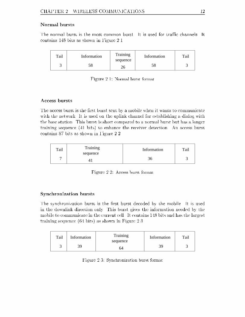
Normal bursts
The normal burst is the most common burst. It is used for tra�c channels. It
contains 148 bits as shown in Figure 2.1.
Tail
3 26
Information
58
Tail
3
Information
58
Trainingsequence
Figure 2.1: Normal burst format
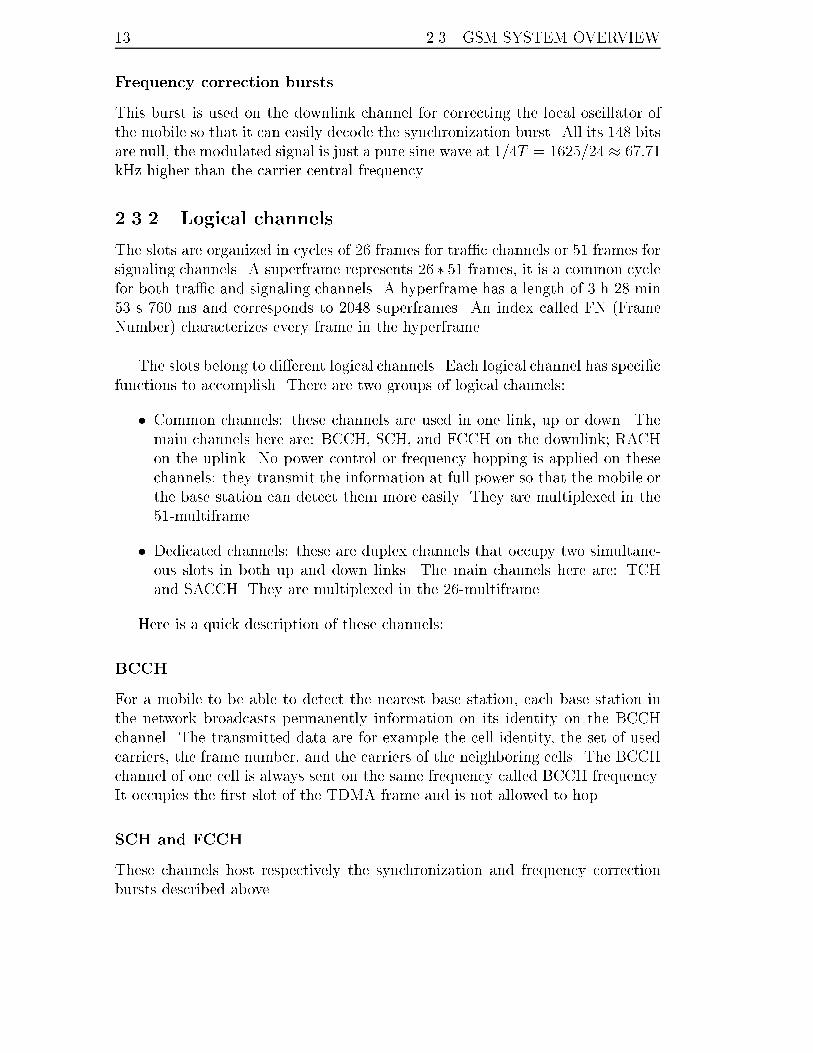
Access bursts
The access burst is the �rst burst sent by a mobile when it wants to communicate
with the network. It is used on the uplink channel for establishing a dialog with
the base station. This burst is short compared to a normal burst but has a longer
training sequence (41 bits) to enhance the receiver detection. An access burst
contains 87 bits as shown in Figure 2.2.
Tail
7
Tail
3
Trainingsequence
Information
3641
Figure 2.2: Access burst format
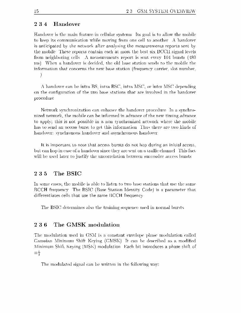
Synchronization bursts
The synchronization burst is the �rst burst decoded by the mobile. It is used
in the downlink direction only. This burst gives the information needed by the
mobile to communicate in the current cell. It contains 148 bits and has the largest
training sequence (64 bits) as shown in Figure 2.3.
Tail
3
Tail
3
Trainingsequence
64
Information
39
Information
39
Figure 2.3: Synchronization burst format
13 2.3. GSM SYSTEM OVERVIEW
Frequency correction bursts
This burst is used on the downlink channel for correcting the local oscillator of
the mobile so that it can easily decode the synchronization burst. All its 148 bits
are null, the modulated signal is just a pure sine wave at 1=4T = 1625=24 � 67:71
kHz higher than the carrier central frequency.
2.3.2 Logical channels
The slots are organized in cycles of 26 frames for tra�c channels or 51 frames for
signaling channels. A superframe represents 26 � 51 frames, it is a common cycle
for both tra�c and signaling channels. A hyperframe has a length of 3 h 28 min
53 s 760 ms and corresponds to 2048 superframes. An index called FN (Frame
Number) characterizes every frame in the hyperframe.
The slots belong to di�erent logical channels. Each logical channel has speci�c
functions to accomplish. There are two groups of logical channels:
� Common channels: these channels are used in one link, up or down. The
main channels here are: BCCH, SCH, and FCCH on the downlink; RACH
on the uplink. No power control or frequency hopping is applied on these
channels: they transmit the information at full power so that the mobile or
the base station can detect them more easily. They are multiplexed in the
51-multiframe.
� Dedicated channels: these are duplex channels that occupy two simultane-
ous slots in both up and down links. The main channels here are: TCH
and SACCH. They are multiplexed in the 26-multiframe.
Here is a quick description of these channels:
BCCH
For a mobile to be able to detect the nearest base station, each base station in
the network broadcasts permanently information on its identity on the BCCH
channel. The transmitted data are for example the cell identity, the set of used
carriers, the frame number, and the carriers of the neighboring cells. The BCCH
channel of one cell is always sent on the same frequency called BCCH frequency.
It occupies the �rst slot of the TDMA frame and is not allowed to hop.
SCH and FCCH
These channels host respectively the synchronization and frequency correction
bursts described above.

CHAPTER 2. WIRELESS COMMUNICATIONS 14
RACH and the Timing Advance parameter (TA)
This channel hosts the access burst. An access burst is sent whenever the mobile
requests a connection. As access to this channel is random by de�nition, it is
subject to collision when two mobiles use the same slot. In this case, the mobile
reiterates its request after a random delay. The protocol used for re-transmission
is inspired from the Aloha protocol.
The propagation delay of one burst is not negligible compared to the bit period
(48=13 � 3:69�s). One bit period corresponds to 1108 meters of propagation. In
normal bursts, the 8.25 guard bit periods (156.25 - 148 ) may not be enough and
the burst could overlap next slot. Bursts in GSM are transmitted in advance so
that they arrive inside the corresponding slot. The advance in time, also called
timing advance (TA), is computed using access bursts. These burst are short
enough so that they cannot overlap the next slot. The time of arrival of this
burst at the base station corresponds to twice the propagation time between the
base station and the mobile. The TA parameter is sent to the mobile so that it
anticipates its transmission. It is coded in 6 bits and has 64 possible values that
correspond to how many half bit periods of propagation separate the base station
from the mobile. The precision of this value is therefore equal to one quarter of a
bit period. This corresponds to 277 meters of wave propagation. Although this
precision is low, it is quite enough to avoid any problem of overlapping between
two consecutive bursts of di�erent users. This parameter can also be used to
enhance the location procedure since it provides a distance information; this will
be discussed later.
TCH and SACCH
The TCH channel is the channel that transmits the tra�c data on both links at
13.6 kb/s. The SACCH channel is the signaling channel that is associated to one
TCH channel.
2.3.3 Location Area Code (LAC)
When the mobile is requested by the network, a search procedure is operated on
a set of cells called location area. At any time, the network knows in which LAC
the mobile is. Indeed, the mobile sends this information to the network at regular
intervals and every time it enters a new LAC. This procedure is called location
update. The LAC informations of all subscribers are stored in huge databases
called Home Location Register (HLR) and Visitor Location Register (VLR).
15 2.3. GSM SYSTEM OVERVIEW
2.3.4 Handover
Handover is the main feature in cellular systems. Its goal is to allow the mobile
to keep its communication while moving from one cell to another. A handover
is anticipated by the network after analyzing the measurements reports sent by
the mobile. These reports contain each at most the best six BCCH signal levels
from neighboring cells. A measurements report is sent every 104 bursts (480
ms). When a handover is decided, the old base station sends to the mobile the
information that concerns the new base station (frequency carrier, slot number,
. . . ).
A handover can be intra BS, intra BSC, intra MSC, or inter MSC depending
on the con�guration of the two base stations that are involved in the handover
procedure.
Network synchronization can enhance the handover procedure. In a synchro-
nized network, the mobile can be informed in advance of the new timing advance
to apply; this is not possible in a non synchronized network where the mobile
has to send an access burst to get this information. Thus there are two kinds of
handover: synchronous handover and asynchronous handover.
It is important to note that access bursts do not hop during an initial access,
but can hop in case of a handover since they are sent on a tra�c channel. This fact
will be used later to justify the uncorrelation between successive access bursts.
2.3.5 The BSIC
In some cases, the mobile is able to listen to two base stations that use the same
BCCH frequency. The BSIC (Base Station Identity Code) is a parameter that
di�erentiates cells that use the same BCCH frequency.
The BSIC determines also the training sequence used in normal bursts.
2.3.6 The GMSK modulation
The modulation used in GSM is a constant envelope phase modulation called
Gaussian Minimum Shift Keying (GMSK). It can be described as a modi�ed
Minimum Shift Keying (MSK) modulation. Each bit introduces a phase shift of
��
2.
The modulated signal can be written in the following way:
CHAPTER 2. WIRELESS COMMUNICATIONS 16
s(t) =
s2Eb
Tej[2�f0t+�(t)] (2.8)
where Eb is the bit energy, T the bit period, and f0 the carrier frequency. The
phase variation �(t) can be written as:
�(t) = �0 +Xi
bi�(t� iT )
bi are the transmitted bits after di�erential coding:
bi = didi�1
and �(t) the modulation function:
�(t) =�
2
Zt
�1se(�)d�
In the MSK, the function se(t) is a rectangular window. The phase variation
is continuous but not smooth enough. In the GMSK modulation, to reduce the
spectrum occupancy, this window is �ltered by a Gaussian function:
se(t) = rect
�t
T
�?
1p2��T
e�t2
2�2T2 (2.9)
with � =
pln 2
2�BTand BT = 0:3.
�(t) can be written more simply with one integral by noticing that [5]:
d�(x)
dx=�
2
Zx+T=2
x�T=2
1p2��
e�t2
2�2 dt
We obtain therefore:8>>><>>>:�(x) = �
2[ (x+ T=2)� (x� T=2)]
(x) = �p2�e�
x2
2�2 + xZ
x
�1
1p2��
e�t2
2�2 dt(2.10)
The drawback of the GMSK modulation compared to the MSK is that it
introduces more inter symbol interference (ISI): the equalization is then a little
more complex.
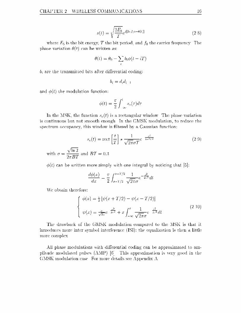
All phase modulations with di�erential coding can be approximated to am-
plitude modulated pulses (AMP) [6]. This approximation is very good in the
GMSK modulation case. For more details see Appendix A.
17 2.3. GSM SYSTEM OVERVIEW
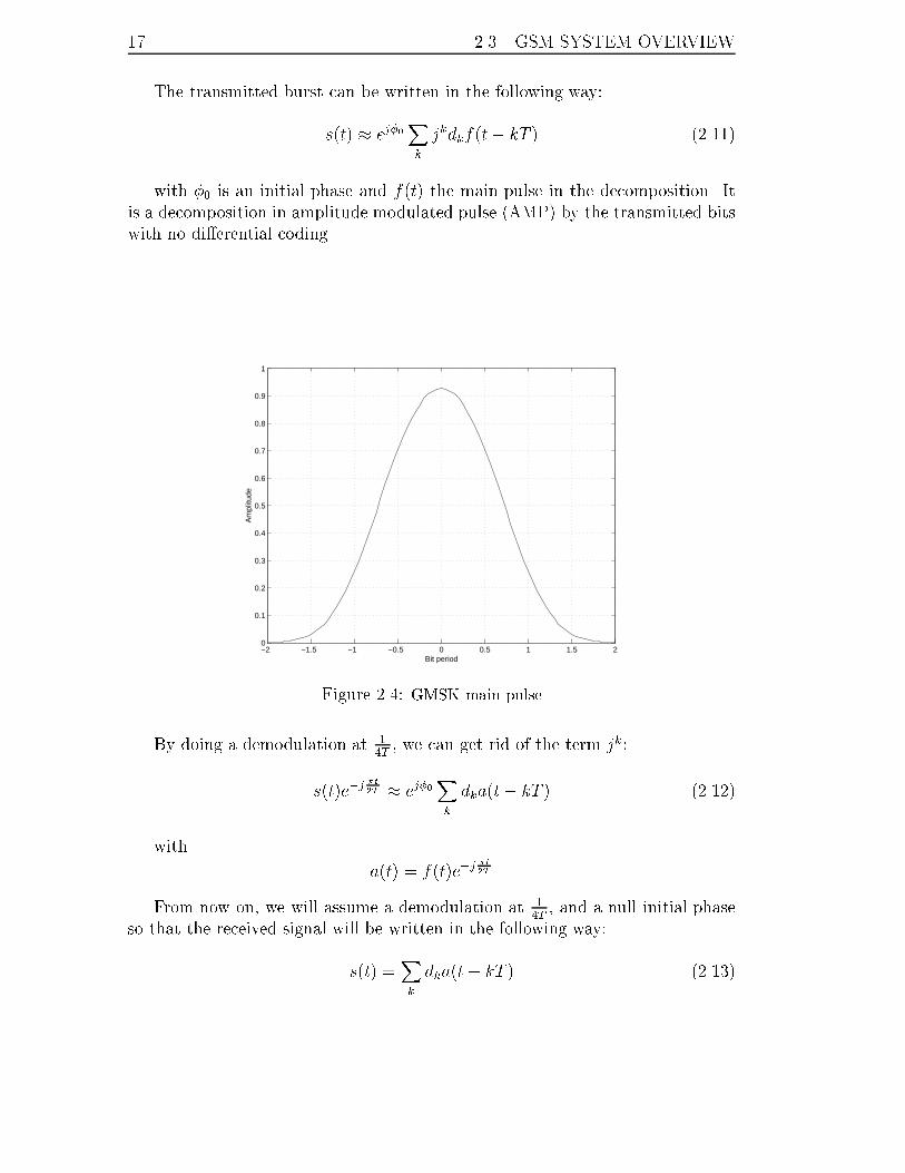
The transmitted burst can be written in the following way:
s(t) � ej�0Xk
jkdkf(t� kT ) (2.11)
with �0 is an initial phase and f(t) the main pulse in the decomposition. It
is a decomposition in amplitude modulated pulse (AMP) by the transmitted bits
with no di�erential coding.
−2 −1.5 −1 −0.5 0 0.5 1 1.5 20
0.1
0.2
0.3
0.4
0.5
0.6
0.7
0.8
0.9
1
Bit period
Am
plitu
de
Figure 2.4: GMSK main pulse
By doing a demodulation at 14T, we can get rid of the term jk:
s(t)e�j�t
2T � ej�0Xk
dka(t� kT ) (2.12)
with
a(t) = f(t)e�j�t
2T
From now on, we will assume a demodulation at 14T, and a null initial phase
so that the received signal will be written in the following way:
s(t) =Xk
dka(t� kT ) (2.13)

CHAPTER 2. WIRELESS COMMUNICATIONS 18
2.4 Channel equalization
The goal of equalization is to reduce the inter symbol interference (ISI) in order
to estimate the transmitted bit. Indeed, since the GMSK main pulse duration is
four times the bit period, inter symbol interference is unavoidable.
At the reception, the received signal is the convolution of the transmitted
signals with a cascade of �lters which are:
� the modulation pulse shape a(t),
� the transmission �lter Fe(t) that �ts the signal to the desired bandwidth,
� the �lter C(t) that corresponds to the propagation over the air,
� The reception �lter Fr(t) that translates the signal to its base-band version.
The channel impulse response is de�ned as the cascade of these �lters. The
transmission scheme can then be written in the following way:
8>>><>>>:y(t) = s(t) ? h(t) + b(t)
s(t) =P
k dk�(t� kT )
h(t) = a(t) ? Fe(t) ? C(t) ? Fr(t)
(2.14)
where y(t) is the received signal, s(t) is the transmitted signal, �(t) the Dirac
function, and b(t) an additive complex noise that is usually assumed to be zero
mean and uncorrelated with s(t):
E[s(t)b(�)] = 0
h(t) is the channel impulse response. For convenience, h(t) is assumed to
have a �nite duration of p bit periods. p is the memory of the channel. One
consequence of Shannon's work is the sampling theorem which states that it is
possible to reconstruct any �nite bandwidth signal from its samples at a rate that
is greater or equal to twice its highest frequency.
In the GSM case, the bandwidth of each carrier is 200 kHz, so that the complex
envelope is limited to 100 kHz. The bit rate, that is approximately equal to 271
kHz is then enough to satisfy the Shannon's criterion. From now on, all signals
are sampled at the bit rate. The sampled signal is:
y(jT ) =p�1Xk=0
h(kT )dj�k + b(jT ) p � j � N (2.15)

19 2.4. CHANNEL EQUALIZATION
The last equation can then be written in a more compact formula using ma-
trices:
Y = D(d)H+B (2.16)
where d = [d1 � � �dq]T refers to the bits of the training sequence,
H = [h(0) � � �h((p� 1)T )]T
Y = [y(pT ) � � �y(qT )]T
B = [b(pT ) � � � b(qT )]T p < q
and:
D(d) =
0BBBB@
dp dp�2 � � � d1dp+1 dp � � � d2...
......
dq dq�1 � � � dm
1CCCCA (2.17)
The noise samples are assumed to be uncorrelated between each other, i.e.
E[BB�] = �2I.
One way of estimating the bits is the maximum likelihood (ML) detector. This
detector is obtained by maximizing the likelihood of the observation with respect
to the parameter to be estimated or equivalently by maximizing the log-likelihood
of the observation:
� = argmax ln p(yj�)
In our case, � is a vector that contains the channel impulse response coe�cients
and the unknown bits. In the context of Gaussian noise, the log-likelihood can
be written in the following way:
ln p(YjH;d) = � 1
�2kY �D(d)Hk2 (2.18)
Several approaches are possible to solve the equation. The channel impulse
response is unknown. It is possible to estimate it directly without any prior
knowledge of the bits: this is called blind equalization. We will focus on the
GSM case where a training sequence consisting of known bits is available in all
bursts.
We will solve the system (2.18) in two steps: in the �rst step, we assume
that d refers to the training sequence and estimate the channel impulse response
accordingly. In the second step, d refers to the unknown bits and the channel
impulse response estimated from the �rst step is used.
CHAPTER 2. WIRELESS COMMUNICATIONS 20
It should be noted that this scenario is not optimal since the estimations of
the unknown bits and the channel impulse response are not performed jointly.
However, the low gain in performances given by the joint estimation does not
justify its huge complexity increase.
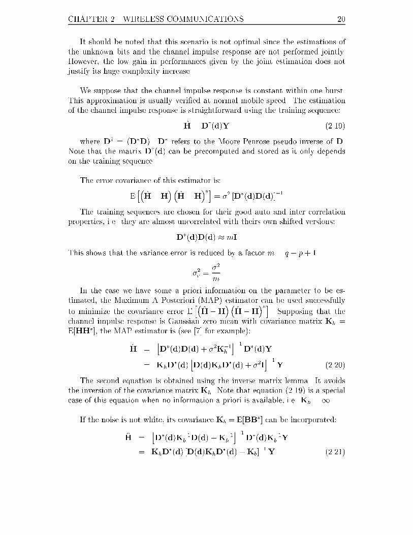
We suppose that the channel impulse response is constant within one burst.
This approximation is usually veri�ed at normal mobile speed. The estimation
of the channel impulse response is straightforward using the training sequence:
H = Dy(d)Y (2.19)
where Dy = (D�D)�1D� refers to the Moore-Penrose pseudo-inverse of D.
Note that the matrix Dy(d) can be precomputed and stored as it only depends
on the training sequence.
The error covariance of this estimator is:
Eh�H�H
� �H�H
��i= �2 [D�(d)D(d)]
�1
The training sequences are chosen for their good auto and inter correlation
properties, i.e. they are almost uncorrelated with theirs own shifted versions:
D�(d)D(d) � mI
This shows that the variance error is reduced by a factor m = q � p+ 1.
�2r=�2
m
In the case we have some a priori information on the parameter to be es-
timated, the Maximum A Posteriori (MAP) estimator can be used successfully
to minimize the covariance error Eh�H�H
� �H�H
��i. Supposing that the
channel impulse response is Gaussian zero mean with covariance matrix Kh =
E[HH�], the MAP estimator is (see [7] for example):
H =hD�(d)D(d) + �2K�1
h
i�1D�(d)Y
= KhD�(d)
hD(d)KhD
�(d) + �2Ii�1
Y (2.20)
The second equation is obtained using the inverse matrix lemma. It avoids
the inversion of the covariance matrix Kh. Note that equation (2.19) is a special
case of this equation when no information a priori is available, i.e. Kh =1.
If the noise is not white, its covariance Kb = E[BB�] can be incorporated:
H =hD�(d)K�1
bD(d) +K�1
h
i�1D�(d)K�1
bY
= KhD�(d) [D(d)KhD
�(d) +Kb]�1Y (2.21)
21 2.4. CHANNEL EQUALIZATION
Once the channel impulse response is estimated, we estimate the unknown
bits by minimizing:
ln p(Yjd) � kY �D(d)Hk2
where d represents in this case the unknown bits. The well known Viterbi
algorithm [8] is usually used here to recursively estimate the unknown bits. This
algorithm can also provide soft con�dence values for each bit enabling soft de-
coding.

CHAPTER 2. WIRELESS COMMUNICATIONS 22
Chapter 3
Technologies for location
This chapter presents a description of possible technologies that might be used
for locating a mobile handset in a radio cellular network. It explains why the
best technology in the actual context is based on time of arrival.
In general, the idea is to gather as many measurements as possible and to
exploit a large number of relevant observations. Each observation contributes to
add some more information and enhances therefore the estimation accuracy. The
set of relevant measurements can be obtained at the handset from signals coming
from di�erent base stations or can be measured from the signal coming from the
mobile and impinging on several base stations. Accumulating both measurements
(i.e. on downlink and uplink channels) enhances the �nal estimation accuracy.
3.1 Distance estimation from signal strength
This is the most intuitive technique to locate a handset. The mobile measures the
signal strength from several base stations. A good candidate is the BCCH channel
since it is transmitted at full power. The mobile can compute the distance that
separates it from the base station by means of an appropriate path loss empirical
model. In general, the path loss is proportional to the distance between the
mobile and the base station :
Pr
Pt= cd� (3.1)
Two distances are required for locating a handset by a simple circular trilateration1.
This methodology has been analyzed in [9]. The main advantage of this method
is that it can easily be implemented in GSM2. Indeed, the mobile sends a mea-
1The ambiguity can be solved by selecting the intersection that is inside the area of interest.2Some operators have already implemented this technology for some commercial applications
such as home zone billing.
23
CHAPTER 3. TECHNOLOGIES FOR LOCATION 24
surements report every 0.48 s that includes the downlink signal levels of the best
six base stations. The signal power level is expressed on a discrete scale running
from 0 to 63.
The main drawback of this method is its low precision due mainly to shad-
owing. However it may be assisted by a prediction map in order to correct the
estimation resulting from the trilateration alone. Such prediction maps are avail-
able in the database of an operator. They are generally obtained by simulation.
Another way of assisting the method is to provide collected �eld measurements
as training data; this is subject of next section.
3.2 Pattern matching based on training data
This technique can be compared to pattern recognition in the sense that the mo-
bile position is assigned to a small area (smaller than a cell). This assignment
decision is made by matching some observations to some prediction maps. The
area of interest is divided into a large number of small areas of location. This
methodology requires a large amount of collected data, which are used to build a
decision model based on some information criterion. This technique is in contrast
with the others in the sense that the location computation is not performed by
trilateration; it is purely statistical. The handset is assigned an area where its
probability of presence is high enough.
Many methods exist to build the decision model based on which the location
area is decided. Decision trees [10] represent one powerful tool for this purpose.
3.3 Angle of Arrival (AoA) estimation
It is perhaps one of the most famous techniques for source localization. This topic
received a lot of interest in the last two decades [11]. The research led to some
well-known algorithms. The problem of interest is to locate multiple coherent or
non coherent sources that impinge on an array consisting of multiple sensors.
Estimating the angle of arrival of a signal requires antenna array. This equip-
ment is expensive and current GSM operators are generally not willing to use
such installations. For this reason, this technique will be omitted for further
considerations.

25 3.4. TIME OF ARRIVAL (TOA) ESTIMATION
3.4 Time of Arrival (ToA) estimation
The estimation of the time of arrival (ToA) parameter is an old technique used in
various applications such as radar and sonar data processing, geological acoustic
sounding, and medical imaging processing. In the GSM context, the ToA esti-
mation can be achieved by means of the training sequence. Two scenarios are
possible, uplink or downlink:
� The mobile estimates the ToA of the training sequence from bursts coming
from di�erent base stations. Synchronization bursts are good candidates
since they have the longest training sequence (64 bits) and are sent at
full power. Moreover, consecutive synchronization bursts are spaced by
10 TDMA frames o�ering better uncorrelation between bursts. The time
needed to observe 20 synchronization is 0.96 s. This method requires mod-
i�cations to actual mobile handsets so that they are able to estimate the
ToA parameter with a better accuracy.
� Several base stations measure the same signal coming from the mobile hand-
set. Since tra�c bursts are subject to power control, access bursts are the
best candidates in this approach. They are always transmitted at full power
and have a long training sequence (41 bits). However, access bursts are sent
only at the beginning of a communication or whenever a handover occurs3.
A scenario suggested by Ericsson is to force the mobile to perform an in-
tra cell handover so that the mobile send an access burst to retrieve the
new link information such as power control and timing advance. The base
station does not respond to this handover and the mobile reiterates its de-
mand. Overall, the mobile sends a high number of access bursts (exactly
70 bursts within 0.32 s) that are measured at several base stations. This
method does not require any modi�cation to the mobile handset4. It makes
use of diversity to increase the number of samples according to the diversity
order. The main drawback is its huge complexity on the network side and
that it cannot work in idle mode. Note that in this special case, access
bursts are allowed to hop since they are sent on a tra�c channel. They are
then assumed to be uncorrelated between each other.
In both scenarios, the main source of error is multipath. The goal of time of
arrival estimation is to detect a path that is as close as possible to the direct line
of sight path. It is however impossible to avoid bias in a time of arrival estimation
when the direct line of sight path is not present.
At least three times of arrival are required if the location is done in two di-
mensions. The unknown variables are x, y, and tr which is an unknown reference
3In the case of asynchronous handover only.4This is not really true since some handsets does not support intra cell handover.
CHAPTER 3. TECHNOLOGIES FOR LOCATION 26
time that will be discussed in Chapter 5. The trilateration is called hyperbolic
because it is based on Di�erence Times of Arrival (DToA) which corresponds to
the equation of a hyperbola. The DToA technology has the advantage of elimi-
nating constant biases that may be present in the ToA estimation.
Base station synchronization is always required for the location to be possible.
The di�erences in transmission times between al base stations (also called RTD
for Real Time Di�erence) involved in the procedure are required. This will be
discussed in Chapter 6.
As the main source of problems in the ToA estimation is multipath, the perfor-
mances are slightly sensitive to the signal-to-noise ratio. A ToA can be measured
even at low signal-to-noise ratios once the training sequence is located. In the
downlink scenario, the detection probability can be enhanced by communicating
the handset prior information on the synchronization state of the neighboring
base stations. This can give some compensation to the limitation of the handset
compared to the base station sensibility and the advantage that it avoids for the
handset the BSIC decoding (see Section 2.3.5) that is required to identify the
base station the handset is measuring.
3.5 Hybrid methods - Joint Angle and Delay
Estimation (JADE)
The method is a combination of both ToA and AoA estimation. The estimation
is performed jointly. The joint estimation enhances signi�cantly the delays esti-
mation. Indeed, two closely spaced (in time) paths may have two di�erent angles
and therefore be easily resolved [12{14].
3.6 Conclusion
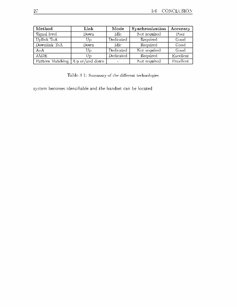
The discussed approaches are shown brie y in Table 3.1. The discussion on
accuracy might be subjective since the approaches have not been tested at all
until now (except the signal level approach). Our preference goes to the ToA
approaches (downlink or uplink) since it seems to give an acceptable accuracy
with some few modi�cations to the mobile handsets and the network.
From now on, we will not distinguish between the downlink or the uplink
time of arrival technologies since these two approaches are strictly identical from
a calculation point of view. Three base stations at least must be involved in the
location procedure in order to obtain three independent times of arrival. Assum-
ing that the di�erences of transmission times of the base stations are known, the
27 3.6. CONCLUSION
Method Link Mode Synchronization Accuracy
Signal level Down Idle Not required Poor
Uplink ToA Up Dedicated Required Good
Downlink ToA Down Idle Required Good
AoA Up Dedicated Not required Good
JADE Up Dedicated Required Excellent
Pattern Matching Up or/and down - Not required Excellent
Table 3.1: Summary of the di�erent technologies
system becomes identi�able and the handset can be located.

CHAPTER 3. TECHNOLOGIES FOR LOCATION 28

Chapter 4
Time of arrival estimation
In this chapter, array processing techniques are applied to the general problem
of temporal analysis of a received narrow band signal consisting of replicas of a
known shape. This signal is received on one single sensor. We are in particular
interested in the estimation of the time of arrival (ToA), which is by de�nition the
time delay of the �rst path. For this purpose, we apply high resolution methods
for estimating all delays and then decide to retain the �rst one as the time of
arrival. We will apply the results to GSM.
The goal is to determine the time delay that is as close as possible to the line
of sight (LOS) path. The main obstacle to time of arrival estimation is multipath.
When the paths are closely spaced, it is hard to resolve them with a wide pulse
shape such as the GMSK pulse. Moreover the line of sight path may not exist
and it is impossible in this case to avoid a bias in the estimation. In [15], it has
been noticed that allowing biases in the estimator can reduce consequently the
variance error.
4.1 Notations and assumptions
In wireless communications, the channel impulse response varies in time due to
mobility. In a Time Division Multiple Access (TDMA) system with short bursts
such as GSM, we can assume that the channel impulse response is constant within
one burst for normal mobile speed since the coherence time is longer than the
burst duration (in GSM 577 �s). In addition, the bursts are uncorrelated from
one burst to another. This is due to frequency hopping1 and, for high mobile
speed, to the coherence time that is shorter than the length of one TDMA frame
(4.615 ms in GSM).
1On tra�c channels only.
29
CHAPTER 4. TIME OF ARRIVAL ESTIMATION 30
The channel impulse response is estimated by means of the known training
sequence (TSC). In GSM, such training sequences are composed of 26 bits in
normal bursts, 64 bits for synchronization bursts, and 41 bits for access bursts
(see Section 2.3.1). They are located in the middle of the burst.
We use the following constants:
� q refers to the length of the training sequence,
� p refers to the channel impulse response length,
� L refers to the number of successive observations2.
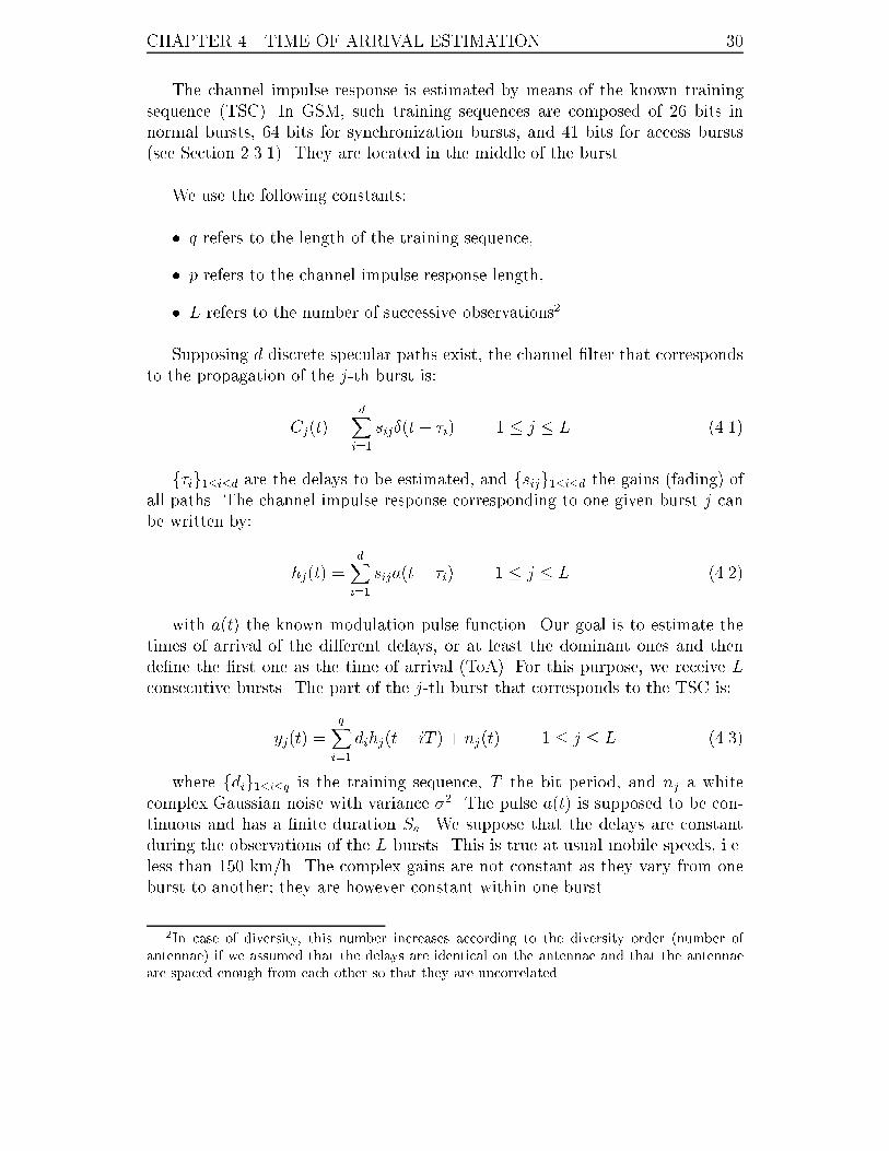
Supposing d discrete specular paths exist, the channel �lter that corresponds
to the propagation of the j-th burst is:
Cj(t) =dX
i=1
sij�(t� �i) 1 � j � L (4.1)
f�ig1�i�d are the delays to be estimated, and fsijg1�i�d the gains (fading) ofall paths. The channel impulse response corresponding to one given burst j can
be written by:
hj(t) =dX
i=1
sija(t� �i) 1 � j � L (4.2)
with a(t) the known modulation pulse function. Our goal is to estimate the
times of arrival of the di�erent delays, or at least the dominant ones and then
de�ne the �rst one as the time of arrival (ToA). For this purpose, we receive L
consecutive bursts. The part of the j-th burst that corresponds to the TSC is:
yj(t) =qX
i=1
dihj(t� iT ) + nj(t) 1 � j � L (4.3)
where fdig1�i�q is the training sequence, T the bit period, and nj a white
complex Gaussian noise with variance �2. The pulse a(t) is supposed to be con-
tinuous and has a �nite duration Sa. We suppose that the delays are constant
during the observations of the L bursts. This is true at usual mobile speeds, i.e.
less than 150 km/h. The complex gains are not constant as they vary from one
burst to another; they are however constant within one burst.
2In case of diversity, this number increases according to the diversity order (number of
antennae) if we assumed that the delays are identical on the antennae and that the antennae
are spaced enough from each other so that they are uncorrelated.

31 4.1. NOTATIONS AND ASSUMPTIONS
All signals are sampled at the bit rate which satis�es the Nyquist/Shannon
criterion3.
In general, the number of delays is unknown but it can be estimated by several
techniques as shown in [16{22]. These techniques are mainly the AIC and MDL
criteria.
We will use the following notations:
a(�i) = [a(��i) � � �a((p� 1)T � �i)]T sampled pulse shifted by �i,
� = (�1 � � � �d) delays to be estimated,
A(�) = [a(�1) � � �a(�d)] rectangular p� d matrix,
Yj = [yj(pT ) � � �yj(qT )]T observations in one burst,
Hj = [hj(0) � � �hj((p� 1)T )]T channel impulse response,
Sj = [s1j � � � sdj]T gains in burst j,
Nj = [nj(pT ) � � �nj(qT )]T noise vector,
Ky = EhYjY
�j
isignal covariance matrix,
Ks = EhSjS
�j
igain covariance matrix,
Kh = EhHjH
�j
ichannel covariance matrix.
We note m = q � p + 1 the number of signal samples of yj(t). The pulse
is normalized, i.e. a�(�)a(�) = 1. The gains are assumed to be Gaussian with
zero mean and uncorrelated in time (from one burst to another), but might be
correlated in space (between the gains of various delays in the same observation).
That is to say:
E [SjS�k] = �jkKs (4.4)
Consequently, the envelope of each gain follows a Rayleigh distribution4. The
uncorrelation in time is well justi�ed if slow frequency hopping is used. The noise
is Gaussian with zero mean, uncorrelated in time and space:
E [NjN�k] = �jk�
2I (4.5)
Let D(d) be the matrix de�ned in (2.17) where d refers to the set of bits
belonging to the training sequence. The observations can be rewritten as:
(Yj = D(d)H
j+Nj
Hj = A(�)Sj1 � j � L (4.6)
3In GSM the bit rate is 270 kHz which is greater than 2� 100 = 200 kHz.4If the line of sight path follows a Ricean distribution then the time of arrival estimation
accuracy is greatly enhanced. We are therefore considering the worst case.
CHAPTER 4. TIME OF ARRIVAL ESTIMATION 32
We can rewrite the observations in a more compact formula:
Yj = D(d)A(�)Sj +Nj 1 � j � L (4.7)
The problem of estimating the delays is then equivalent to the joint estimation
of the angles of arrival of d unknown sources impinging on an array of m sensors
[11, 23, 24]:
�Yj = �A(�)�Sj + �Nj 1 � j � L (4.8)
where �A(�) = [�a(�1) � � � �a(�d)], � denotes the set of the d angles of arrival to
be estimated. The m dimension vector �a(�) is the array spatial signature for a
source coming from direction �. It is also called steering vector. In our case the
steering vector is D(d)a(�).
The di�erences between (4.7) and (4.8) are:
� m is the number of samples instead of the number of sensors,
� the observations Yj are the consecutive samples on one single antenna in-
stead of the array output �Yj,
� the matrix D(d)A(�) depends on the time delays while �A(�) depends on
the angles of arrival. Note that the rank of �A(�) is d and the rank of
D(d)A(�) is equal to min(d; p; q� p). However, this minimum is in general
equal to the number of delays d.
� the random gains �Sj play the role of the sources instead of the gains Sj.
The following de�nitions are useful to evaluate an estimator:
Consistency
An estimator is consistent when it is asymptotically unbiased, i.e. the estimator
tends to the true value when the number of observations tends to in�nity.
E�ciency
An estimator is e�cient if it reaches the Cramer-Rao bound that provides a lower
bound on the variance error of any unbiased estimator. An estimator may not be
e�cient but asymptotically e�cient, i.e. when the number of observations tends
to in�nity, the variance error tends to the asymptotic Cramer-Rao bound.
33 4.2. TEMPORAL APPROACH
4.2 Temporal approach
This approach deals directly with the samples in the time domain while the sec-
ond approach developed in section 4.3 deals with the Fourier transform of the
observations. All results obtained in this section are valid in the frequency do-
main too. As we will see, the frequency approach o�ers new perspectives.
We analyze the general case where the gain covariance matrix Ks is assumed
to be de�nite positive. It is possible to suppose that this matrix is diagonal, i.e.
uncorrelated gains, as done in [25].
It is common to distinguish two maximum likelihood estimators [26]:
4.2.1 The Deterministic Maximum Likelihood (DML)
In this approach, the unknown gains Sj are estimated in addition to the d delays.
We must then perform a joint estimation of the gains in each observation and
the common delays. This approach is interesting if, for some reason, we are not
sure that the gains are Gaussian.
The likelihood to be maximized is:
LYj=1
p(Yjj�;Sj; �2) =1
�L�2Lme� 1
�2
PL
j=1kYj�D(d)A(�)Sjk2 (4.9)
We then have to solve the following problem:
(� ; S1; � � � ; SL; �2) = argmin�
1
�2
LXj=1
kYj �D(d)A(�)Sjk2 + Lm ln�2 (4.10)
A derivation with respect to �2 gives:
�2(�) =1
Lm
LXj=1
kYj �D(d)A(�)Sjk2
Hence, the estimator is given by:
(� ; S1; � � � ; SL) = argmin�
LXj=1
kYj �D(d)A(�)Sjk2 (4.11)
We then have the well-known solution:
Sj(�) = [D(d)A(�)]yYj (4.12)
CHAPTER 4. TIME OF ARRIVAL ESTIMATION 34
�2(�) =Tr(�?
D(d)A(�)Ky)
m(4.13)
�?A
refers to the projection matrix onto the null space of A. Ky is the
estimated covariance matrix by averaging the data:
Ky =1
L
LXj=1
YjY�j
(4.14)
The next step is to maximize with respect to � :
LXj=1
kYj �D(d)A(�) [D(d)A(�)]yYjk2 =
LXj=1
k�?D(d)A(�)Yjk2
=LXj=1
Tr�Y�
j�?D(d)A(�)Yj
�
= L Trh�?D(d)A(�)Ky
i
We have used the fact that �?A�?A= �?
Aand that Tr(AB) = Tr(BA).
Ky is a su�cient statistic for the estimation of the delays. The maximum
likelihood estimate of � is obtained by minimizing the following concentrated
function:
VDML(�) = Trh�?D(d)A(�)Ky
i(4.15)
This estimator is known to be ine�cient [27], in the sense that it does not reach
the Cramer-Rao bound. This is not surprising since the number of parameters to
be estimated increases with the number of realizations. For L observations, we
have to estimate L(d + 1) parameters. It is straightforward to see, for example,
that �2(�) in (4.13) is biased since:
E[�2(�)] =m� d
m�2
4.2.2 The Stochastic Maximum Likelihood (SML)
In this approach, we estimate � without estimating the gains. Yj is Gaussian as
it is a linear sum of Gaussian variables. The quantity to be maximized is:
LYj=1
p(Yjj�;Ks; �2) =
exph�LTr(KyK
�1y)i
�Lm jKyjL(4.16)
with:
Ky = A(�)KsA�(�) + �2I (4.17)
35 4.2. TEMPORAL APPROACH
In this case, Ky is a su�cient statistic for the estimation of both � and Ks.
The stochastic maximum likelihood estimator is given by:
(� ; Ks; �2) = arg max
�;Ks;�2TrhKyK
�1y
i+ ln jKyj (4.18)
Ks and �2 can be eliminated and � is obtained by minimizing the following
cost function [28]:
VSML(�) = ln���D(d)A(�)Ks(�) [D(d)A(�)]
�+ �2(�)I
��� (4.19)
with,
Ks(�) = [D(d)A(�)]y(Ky � �2(�)I) [D(d)A(�)]
y�(4.20)
�2(�) =Tr��?D(d)A(�)Ky
�m� d
(4.21)
Unlike DML, SML is known to be consistent and asymptotically e�cient [26].
It is usually called unconstrainted maximum likelihood because the estimation of
Ks has been performed without the constraint that it must be positive de�nite.
In some cases Ks(�) given by (4.20) may be inde�nite. Taking into account such
constraint is complex [29]. Moreover, the estimator that takes this constraint
into account gives asymptotically (i.e. L ! 1) the same performances. Again,
this is due to the e�ciency of SML.
4.2.3 Channel impulse response estimation
According to (4.6), the least squares estimate of Hj is straightforward and given
by:
Hj = Dy(d)Yj (4.22)
The training sequences were designed to have very good autocorrelation prop-
erties, i.e:
D�(d)D(d) � mI (4.23)
If we assume (4.23) to hold with equality5, the least squares estimation of the
channel impulse response has a simple formula:
Hj =D�(d)Yj
m(4.24)
We then have a noisy version of the j-th channel impulse response hj(t):
hj(t) =dX
i=1
sija(t� �i) + wj(t) 1 � j � L (4.25)
5In fact, this is impossible for a �nite sequence length, however we will accept this approxi-
mation for the training sequences of access and synchronization bursts.
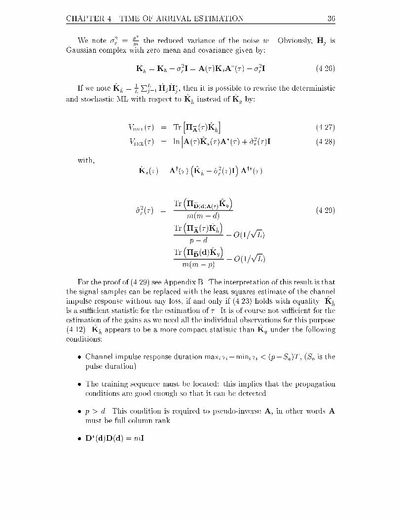
CHAPTER 4. TIME OF ARRIVAL ESTIMATION 36
We note �2r= �2
mthe reduced variance of the noise w. Obviously, Hj is
Gaussian complex with zero mean and covariance given by:
Kh= Kh + �2
rI = A(�)KsA
�(�) + �2rI (4.26)
If we note Kh= 1
L
PL
j=1 HjH�j, then it is possible to rewrite the deterministic
and stochastic ML with respect to Khinstead of Ky by:
VDML(�) = Trh�?A(�)K
h
i(4.27)
VSML(�) = ln���A(�)Ks(�)A
�(�) + �2r(�)I
��� (4.28)
with,
Ks(�) = Ay(�)�K
h� �2
r(�)I
�Ay�(�)
�2r(�) =
Tr��?D(d)A(�)Ky
�m(m� d)
(4.29)
=Tr��?A(�)K
h
�p� d
+O(1=pL)
=Tr��?D(d)Ky
�m(m� p)
+O(1=pL)
For the proof of (4.29) see Appendix B. The interpretation of this result is that
the signal samples can be replaced with the least squares estimate of the channel
impulse response without any loss, if and only if (4.23) holds with equality. Kh
is a su�cient statistic for the estimation of � . It is of course not su�cient for the
estimation of the gains as we need all the individual observations for this purpose
(4.12). Khappears to be a more compact statistic than Ky under the following
conditions:
� Channel impulse response duration maxi �i�mini �i < (p�Sa)T , (Sa is thepulse duration).
� The training sequence must be located: this implies that the propagation
conditions are good enough so that it can be detected.
� p > d. This condition is required to pseudo-inverse A, in other words A
must be full column rank.
� D�(d)D(d) = mI
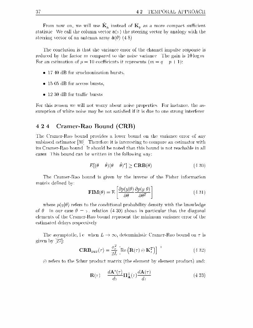
37 4.2. TEMPORAL APPROACH
From now on, we will use Khinstead of Ky as a more compact su�cient
statistic. We call the column vector a(�) the steering vector by analogy with the
steering vector of an antenna array �a(�) (4.8).
The conclusion is that the variance error of the channel impulse response is
reduced by the factor m compared to the noise variance. The gain is 10 logm.
For an estimation of p = 10 coe�cients it represents (m = q � p+ 1):
� 17.40 dB for synchronization bursts,
� 15.05 dB for access bursts,
� 12.30 dB for tra�c bursts.
For this reason we will not worry about noise properties. For instance, the as-
sumption of white noise may be not satis�ed if it is due to one strong interferer.
4.2.4 Cramer-Rao Bound (CRB)
The Cramer-Rao bound provides a lower bound on the variance error of any
unbiased estimator [30]. Therefore it is interesting to compare an estimator with
its Cramer-Rao bound. It should be noted that this bound is not reachable in all
cases. This bound can be written in the following way:
E[(� � �)(� � �)�] � CRB(�) (4.30)
The Cramer-Rao bound is given by the inverse of the Fisher information
matrix de�ned by:
FIM(�) = E
"@p(yj�)@�
@p(yj�)@�T
#(4.31)
where p(yj�) refers to the conditional probability density with the knowledge
of �. In our case � = � , relation (4.30) shows in particular that the diagonal
elements of the Cramer-Rao bound represent the minimum variance error of the
estimated delays respectively.
The asymptotic, i.e. when L!1, deterministic Cramer-Rao bound on � is
given by [27]:
CRBDET(�) =�2r
2L
hRe�R(�)�KT
s
�i�1(4.32)
� refers to the Schur product matrix (the element by element product) and:
R(�) =dA�(�)
d��?A(�)
dA(�)
d�(4.33)
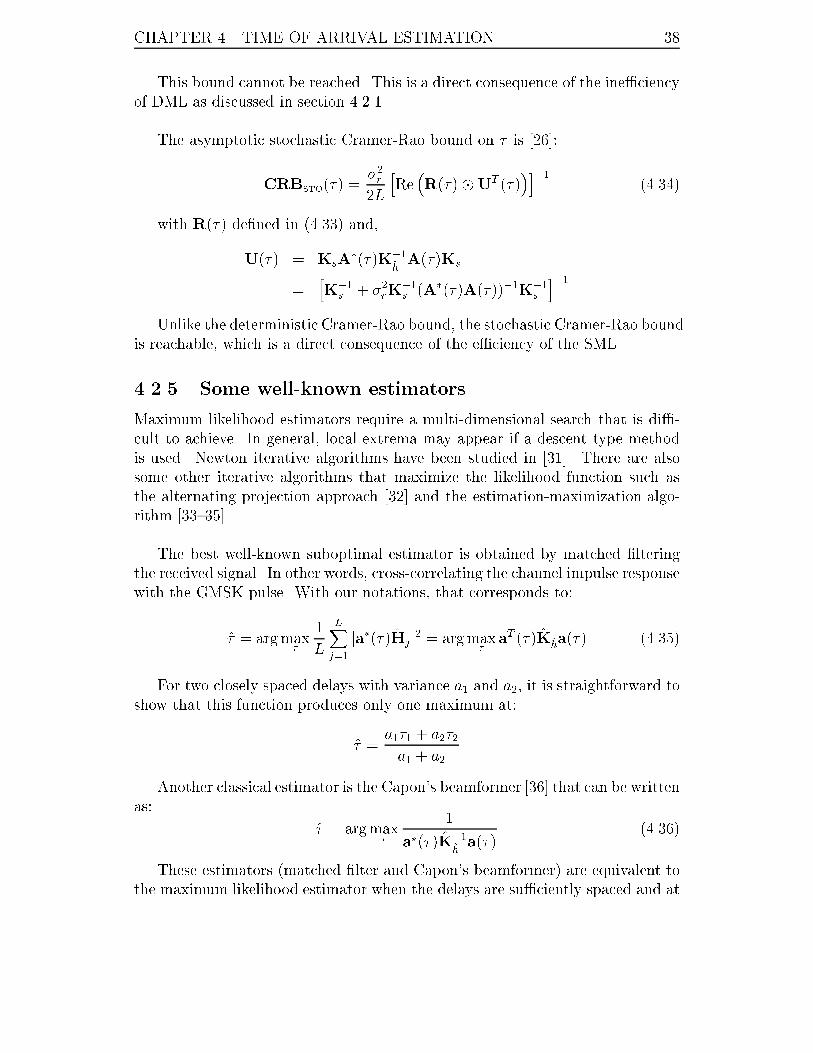
CHAPTER 4. TIME OF ARRIVAL ESTIMATION 38
This bound cannot be reached. This is a direct consequence of the ine�ciency
of DML as discussed in section 4.2.1.
The asymptotic stochastic Cramer-Rao bound on � is [26]:
CRBSTO(�) =�2r
2L
hRe�R(�)�UT (�)
�i�1(4.34)
with R(�) de�ned in (4.33) and,
U(�) = KsA�(�)K�1
hA(�)Ks
=hK�1
s+ �2
rK�1
s(A�(�)A(�))�1K�1
s
i�1Unlike the deterministic Cramer-Rao bound, the stochastic Cramer-Rao bound
is reachable, which is a direct consequence of the e�ciency of the SML.
4.2.5 Some well-known estimators
Maximum likelihood estimators require a multi-dimensional search that is di�-
cult to achieve. In general, local extrema may appear if a descent type method
is used. Newton iterative algorithms have been studied in [31]. There are also
some other iterative algorithms that maximize the likelihood function such as
the alternating projection approach [32] and the estimation-maximization algo-
rithm [33{35].
The best well-known suboptimal estimator is obtained by matched �ltering
the received signal. In other words, cross-correlating the channel impulse response
with the GMSK pulse. With our notations, that corresponds to:
� = argmax�
1
L
LXj=1
ja�(�)Hjj2 = argmax�aT (�)K
ha(�) (4.35)
For two closely spaced delays with variance a1 and a2, it is straightforward to
show that this function produces only one maximum at:
� =a1�1 + a2�2
a1 + a2
Another classical estimator is the Capon's beamformer [36] that can be written
as:
� = argmax�
1
a�(�)K�1ha(�)
(4.36)
These estimators (matched �lter and Capon's beamformer) are equivalent to
the maximum likelihood estimator when the delays are su�ciently spaced and at
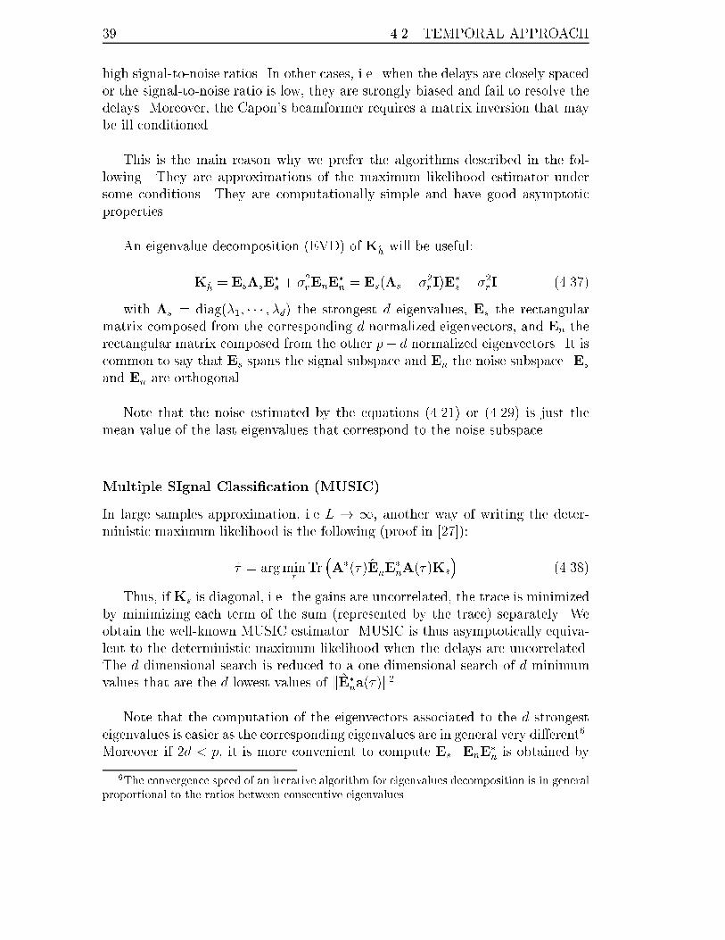
39 4.2. TEMPORAL APPROACH
high signal-to-noise ratios. In other cases, i.e. when the delays are closely spaced
or the signal-to-noise ratio is low, they are strongly biased and fail to resolve the
delays. Moreover, the Capon's beamformer requires a matrix inversion that may
be ill conditioned.
This is the main reason why we prefer the algorithms described in the fol-
lowing. They are approximations of the maximum likelihood estimator under
some conditions. They are computationally simple and have good asymptotic
properties.
An eigenvalue decomposition (EVD) of Khwill be useful:
Kh= Es�sE
�s+ �2
rEnE
�n= Es(�s � �2
rI)E�
s+ �2
rI (4.37)
with �s = diag(�1; � � � ; �d) the strongest d eigenvalues, Es the rectangular
matrix composed from the corresponding d normalized eigenvectors, and En the
rectangular matrix composed from the other p� d normalized eigenvectors. It is
common to say that Es spans the signal subspace and En the noise subspace. Es
and En are orthogonal.
Note that the noise estimated by the equations (4.21) or (4.29) is just the
mean value of the last eigenvalues that correspond to the noise subspace.
Multiple SIgnal Classi�cation (MUSIC)
In large samples approximation, i.e L ! 1, another way of writing the deter-
ministic maximum likelihood is the following (proof in [27]):
� = argmin�
Tr�A�(�)E
nE�nA(�)Ks
�(4.38)
Thus, if Ks is diagonal, i.e. the gains are uncorrelated, the trace is minimized
by minimizing each term of the sum (represented by the trace) separately. We
obtain the well-known MUSIC estimator. MUSIC is thus asymptotically equiva-
lent to the deterministic maximum likelihood when the delays are uncorrelated.
The d dimensional search is reduced to a one dimensional search of d minimum
values that are the d lowest values of kE�na(�)k2.
Note that the computation of the eigenvectors associated to the d strongest
eigenvalues is easier as the corresponding eigenvalues are in general very di�erent6.
Moreover if 2d < p, it is more convenient to compute Es. EnE�nis obtained by
6The convergence speed of an iterative algorithm for eigenvalues decomposition is in general
proportional to the ratios between consecutive eigenvalues.
CHAPTER 4. TIME OF ARRIVAL ESTIMATION 40
I� EsE�s. It is common to search for the d peaks of the following function, also
called MUSIC spectrum:
�(�) =1
a�(�)(I� EsE�s)a(�)
(4.39)
MUSIC has been widely studied in the literature, see [27, 37, 38].
Weight Subspace Fitting (WSF)
This estimator is based on the fact that the range space ofA(�) is the same as Es.
This implies that there is one unique full rank matrix T so that: Es = A(�)T. In
other words, � is the unique vector that satis�es this relation. As Es is corrupted
by noise, �nding the estimate can be formulated in the following way [39{41]:
[� ; T] = argmin�;T
kEsW1
2 �A(�)Tk2 (4.40)
where W is a weighting matrix for the signal subspace.
T can be eliminated easily and the WSF estimator becomes:
� = argmin�
Tr��?A(�)EsWE�
s
�(4.41)
There exists an optimum weighting matrix in the sense that it minimizes the
asymptotic covariance error [39]:
� = argmin�
Tr��?A(�)EsWOPTE
�s
�(4.42)
with,
WOPT = (�s � �2rI)2��1
s(4.43)
This matrix can be replaced in practice with a consistent estimate without
a�ecting the asymptotic properties of the estimator. The corresponding estimator
is a large samples approximation of the stochastic maximum likelihood estimation
[26]. It is e�cient in the sense that its asymptotic covariance corresponds to the
stochastic Cramer-Rao bound (4.34). Note that at high signal-to-noise ratios and
large samples, the deterministic and stochastic maximum likelihood estimators
coincide.
4.3 Frequency approach
4.3.1 Formulation
In this case, we perform exactly the same computations as before but on the
Fourier transform of the observations. We then have from (4.25):
�hj(f) = ~hj(f) = �a(f)
nXi=1
sije�j2��if + �wj(f) 1 � j � L (4.44)
41 4.3. FREQUENCY APPROACH
�(:) denotes the Fourier transform of (:), w is a complex Gaussian noise with
reduced variance �2r= �2
m.
We take the same number of samples as in the temporal domain, i.e. p
samples. Let the set of frequencies of these samples be f = (f1; � � � ; fp) on the
nonzero support of �a(f). We can then express the observations in the following
way:
�Hj = ~Hj = �( ) ~A(�)Sj + �Wj 1 � j � L (4.45)
with �( ) = diag( ), = [�a(f1) � � � �a(fp)]T and:
~A(�) =
0BB@e�2�jf1�1 � � � e�2�jf1�d
......
e�2�jfp�1 � � � e�2�jfp�d
1CCA
The advantage of this new representation is that it corresponds exactly to
the estimation of the angles of arrival of d sources impinging on a uniform linear
array (ULA) of p sensors (4.8) with di�erent sensor gains [42, 43].
Assuming that the Nyquist/Shannon criterion is satis�ed at the bit rate, the
Fourier transform can be written in the following way:
�Hj = ~Hj = FHj (4.46)
with F being the following p� p matrix:
F = T
0BB@e�2�jf1T � � � e�2�jpf1T
......
e�2�jfpT � � � e�2�jpfpT
1CCA
T is the bit period. Equation (4.45) is similar to (4.7). The noise remains
Gaussian. It is white if F is orthonormal, which is the case if an FFT is used. It
is worth noting here that there are no edge e�ects while performing the FFT on
Hj since in practice p = 10 and pT is about 37 �s which is longer than typical
durations (< 15�s).
The new covariance is:
K~h = FKhF� (4.47)
which gives directly the new covariance K~h from the latter one Kh.
The noise covariance becomes:
K �w = �2rFF� (4.48)
CHAPTER 4. TIME OF ARRIVAL ESTIMATION 42
If the sample frequencies are chosen uniformly, i.e. fi = f1 + (i � 1)�, the
matrix ~A(�) has a Vandermonde structure. For practical reasons, we choose
� = 1pT
so that F becomes an FFT matrix and the noise �Wj remains white. f1is chosen so that the samples are centered, we then have:
� f1 = �fp = �p�12pT
.
� fi =i� p+1
2
pT
� FF� = F�F = I
In this case, the steering vector is �( )~a(�) with:
~a(�) = [e�2�jf1� ; � � � ; e�2�jfp� ]T = e�2�jf1� [1; e�2�j�� ; � � � ; e�2�jp�� ]T (4.49)
It should be noted here that there is no ambiguity on the possible value of �
if and only if the phase range does not exceed 2�, in other words:
0 � 2��� � 2� =) 0 � � � 1
�= pT
This condition is supposed to be veri�ed by the assumptions shown in Sec-
tion 4.2.3.
All algorithms depicted in section 4.2.5 can be applied here too. We can also
use some elegant algorithms taking advantage of the Vandermonde structure of
the matrix ~A(�):
� Root MUSIC: the estimates are obtained by mean of roots of a polynomial
that is related to the noise subspace,
� IQML: an iterative algorithm of successive least squares estimations without
eigen-decomposition,
� Root WSF: the estimates are obtained by means of roots of a polynomial
that will be estimated,
� ESPRIT: this estimator reduces the computations in the sense that it avoids
the search for the maximum of a function (like the MUSIC spectrum func-
tion); the delays are obtained explicitly without search.
These methods are known as parametric methods. They are computationally
attractive because they exploit the Vandermonde structure of ~A(�). In statisti-
cal array processing, this corresponds to the case of uniform linear arrays (ULA)
with known calibration given by the elements of the diagonal matrix �( ).
We note in the following ~Es and ~En the new signal and noise subspace:
K~h =~Es
~�s~E�s+ ~En
~�n~E�n
43 4.3. FREQUENCY APPROACH
4.3.2 Some well-known estimators
Root MUSIC
This algorithm is a variant of MUSIC and can be seen as an extension to the
Pisarenko's approach [44].
MUSIC is de�ned by the d values of � that minimizes the following cost
function:
k ~E�
n�( )~a(�)k2 = k ~E
�
n�( )[1; z; � � � ; zp]Tk2 (4.50)
with z = z(�) = e�j2���, the right side following from (4.49). It is clear that in a
noise free model these values are the d roots of this function that lie on the unit
circle:
zi = e�j2��i� 1 � i � d
The delays are then obtained by means of the argument of these roots:
�i =�12��
arg zi
Since only the values of z on the unit circle are of interest, we can substitute
z� with 1z. The resulting function is a polynomial that can be written in the
following way using the estimated noise subspace:
H(z) =2(p�1)Xk=0
Trk�p
���( ) ~En
~E�
n�( )
�zk (4.51)
where Trk(:) denotes the trace of the k-th diagonal of (:), in particular Tr0(:) is
the trace of (:). In this case the matrix is hermitian and we have Trk(:) = Tr��k(:).
The Root MUSIC estimator is given by taking the argument of the n closest
roots to the unit circle of H(z) that are inside or on the unit circle. Note that
MUSIC is given by the minimum of (4.50) on the unit circle and is therefore
not equivalent to Root MUSIC. It has been shown in [45] that Root MUSIC is
asymptotically equivalent to MUSIC but as all parametric methods, it has a bet-
ter threshold at low signal-to-noise ratios.
Iterative Quadratic Maximum likelihood (IQML) and Root WSF
These two algorithms are based on a di�erent parameterization. Let B(b) be the
following p� (p� d) matrix [46, 47]:
B�(b) =
0BBBBB@
bd � � � b0 0 � � � 0
0 bd � � � b0. . .
......
. . .. . .
. . . 0
0 � � � 0 bd � � � b0
1CCCCCA (4.52)
CHAPTER 4. TIME OF ARRIVAL ESTIMATION 44
where b = [b0 � � � bd]T are the set of coe�cients of the following polynomial:
dXi=0
bizd�i = b0
dYi=1
(z � e�j2��i�) (4.53)
From the de�nition of B(b), B�(b) ~A(�) = 0, and since the rank of B(b) is
by construction p� d, it follows that its columns span the null subspace of ~A(�):
�B(b) = �?~A(�) (4.54)
and,
����B(b) = �?�~A
(�) (4.55)
It is equivalent to estimate b or � as they are directly related. It is however
easier to estimate b if an iterative approach is used. From de�nition (4.52), the
DML criterion (4.27) can be written as:
VDML(b) = Trh����B(b)K~h
i(4.56)
The IQML algorithm is an iterative algorithm that tries to minimize this cost
function iteratively by minimizing the following linear problem at iteration k:
bk = argminb
Tr
�B(b)
hB�(bk�1)�
�1���B(bk�1)i�1
B�(b)��1K~h����
(4.57)
b can be initialized so that B�(b0)��1���B(b0) = I. Each iteration is a
simple least squares estimation. To avoid the trivial solution b = 0, one can add
the constraint that kbk = 1 by normalizing bk at each iteration. One can also
use the fact that the roots lie on the unit circle so that the elements of b must
satisfy the conjugate symmetry constraint:
bi = b�d�i 0 � i � d () Jb = bc (4.58)
This reduces the number of parameters to be estimated. Moreover b should be
constrainted to ensure that the corresponding polynomials has all its zeroes on
the unit circle. However, the gain in performances obtained by taking into ac-
count this constraint is negligible [47].
The advantage of IQML is that it does not require any eigenvalue decompo-
sition. However, it is known to be ine�cient and leads to biased estimates [48].
Recently a modi�ed IQML approach has been proposed [49] which overcomes the
bias of the basic version and is asymptotically e�cient.
Root WSF is a derivation of the WSF estimator. Introducing the matrix
B(b), the WSF criterion becomes:

45 4.3. FREQUENCY APPROACH
b = argminb
Tr
�����B(b) ~Es
~WOPT~E�
s
�(4.59)
with ~WOPT de�ned as in (4.43) by:
~WOPT = (~�s � �2rI)2~��1
s
The same algorithm as for IQML is used. However, in this special case, two it-
erations are enough [11]. This is due to the fact that in this case [B�(b)��1���B(b)]�1
can be replaced with a consistent estimate without a�ecting the asymptotic per-
formances [48].
For minimizing each step, one can use the following formula:
Tr(ABCD) = Vec�(B�)(AT C)Vec(D)
Thus the step described by (4.57) reduces to the minimization of b�Lb with a
constraint on b. The solution is the eigenvector of L associated to the smallest
eigenvalue.
Estimation of Signal Parameters via Rotational Invariance Techniques
(ESPRIT)
The algorithm exploits the Vandermonde structure of ~A(�). ~A(�) satis�es the
following invariance properties [50]:
J1 ~A(�) = J2 ~A(�)�(�) �(�) = diag(e2�j��1 ; � � � ; e2�j��d) (4.60)
where J1 and J2 are selection matrices of the �rst and the last p�1 rows, i.e.:
J1 = [Ip�1 0] J2 = [0 Ip�1]
Our goal is to determine the matrix �(�) which gives explicitly the di�erent
delays. Using the fact that the range space of ~Es is the same as the range space
of �( ) ~A(�), there exists one unique full rank matrix T so that:
J1 ~Es = J1�( ) ~A(�)T J2 ~Es = J2�( ) ~A(�)T
Noting �1 the matrix � after deleting its last row and last column, and �2
the matrix � after deleting its �rst row and �rst column, one can write:
J1 ~Es = �1J1 ~A(�)T J2Es = �2J2 ~A(�)T
Using the invariance properties shown by (4.60), we get:
J1 ~Es = �1J2 ~A(�)�(�)T J2 ~Es = �2J2 ~A(�)T
CHAPTER 4. TIME OF ARRIVAL ESTIMATION 46
It follows that:
�2��11 J1 ~Es = J2 ~Es(t) (4.61)
With (t) = T�1�(�)T. The eigenvalues of (t) directly yield the desired
delays. We have to estimate this matrix. One way of doing that is by least
squares estimation:
(�) =
�J2 ~Es
�y�2�
�11 J1 ~Es
Some algorithms may perform better than least squares: total least squares ES-
PRIT [51], weighted ESPRIT [52], and multiple invariance ESPRIT [53].
4.3.3 Forward-Backward averaging
Forward-Backward averaging is a technique used to virtually double the available
samples. It is based on the following equation which is a direct consequence of
the Vandermonde structure of A(�):
J ~Ac(�) = ~A(�)�
with � = diag(e2�(m�1)�1 ; � � � ; e2�(m�1)�d) and J the anti-identity matrix. We can
de�ne a modi�ed covariance matrix in the following way:
1
2(K~h + JKc
~hJ) =
1
2( ~A(K~h + �Kc
~h��) ~A�) (4.62)
The reason for the appellation "forward-backward" is that while the indices of~Hj run forward (1; 2; � � � ; m) those of J ~Hj run backward (m;m� 1; � � � ; 1). Theconsequence is that the extraction of the signal subspace from this new matrix
correspond to the space spanned by ~A(�).
While Forward-Backward averaging is known to enhance the performance of
some algorithms such as Root MUSIC or ESPRIT [54], it is however shown that
it must not be used for a statistically e�cient method such as Root WSF [55].
4.4 Simulations
In the following, simulations are presented for the simple case of a channel im-
pulse response consisting of two delays equally powered. Synchronization bursts
are used (downlink scenario). The GMSK pulse is �ltered so that it �ts the 200
kHz bandwidth around its carrier. We �ltered it at 1=T , i.e. between �1=2Tand +1=2T � 135 kHz. In Figure 4.1 the GMSK pulse and two �ltered versions
are displayed at 1=T and at 0:8=T . It is shown that while the perfect GMSK
pulse has a duration of 4 bit periods, the �ltered versions duration is longer (8
bit periods at 1=T ). From now on, we will assume in simulations that the pulse
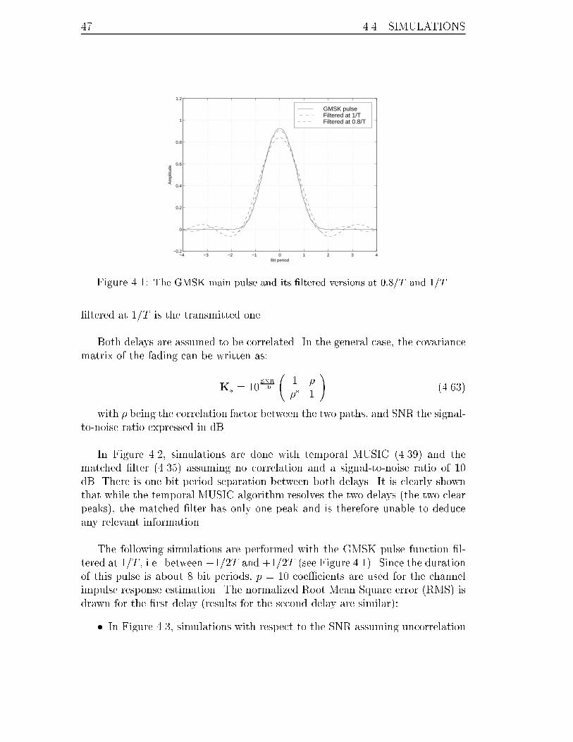
47 4.4. SIMULATIONS
−4 −3 −2 −1 0 1 2 3 4−0.2
0
0.2
0.4
0.6
0.8
1
1.2
Bit period
Am
plitu
de
GMSK pulseFiltered at 1/TFiltered at 0.8/T
Figure 4.1: The GMSK main pulse and its �ltered versions at 0:8=T and 1=T .
�ltered at 1=T is the transmitted one.
Both delays are assumed to be correlated. In the general case, the covariance
matrix of the fading can be written as:
Ks = 10SNR
10
1 �
�� 1
!(4.63)
with � being the correlation factor between the two paths, and SNR the signal-
to-noise ratio expressed in dB.
In Figure 4.2, simulations are done with temporal MUSIC (4.39) and the
matched �lter (4.35) assuming no correlation and a signal-to-noise ratio of 10
dB. There is one bit period separation between both delays. It is clearly shown
that while the temporal MUSIC algorithm resolves the two delays (the two clear
peaks), the matched �lter has only one peak and is therefore unable to deduce
any relevant information.
The following simulations are performed with the GMSK pulse function �l-
tered at 1=T , i.e. between �1=2T and +1=2T (see Figure 4.1). Since the duration
of this pulse is about 8 bit periods, p = 10 coe�cients are used for the channel
impulse response estimation. The normalized Root Mean Square error (RMS) is
drawn for the �rst delay (results for the second delay are similar):
� In Figure 4.3, simulations with respect to the SNR assuming uncorrelation
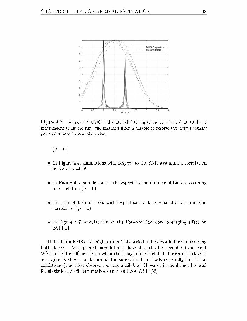
CHAPTER 4. TIME OF ARRIVAL ESTIMATION 48
0 0.5 1 1.5 2 2.5 3 3.5 40
0.1
0.2
0.3
0.4
0.5
0.6
0.7
0.8
0.9
1
Bit period
MUSIC spectrumMatched filter
Figure 4.2: Temporal MUSIC and matched �ltering (cross-correlation) at 10 dB, 5
independent trials are run: the matched �lter is unable to resolve two delays equally
powered spaced by one bit period.
(� = 0).
� In Figure 4.4, simulations with respect to the SNR assuming a correlation
factor of � =0.99.
� In Figure 4.5, simulations with respect to the number of bursts assuming
uncorrelation (� = 0).
� In Figure 4.6, simulations with respect to the delay separation assuming no
correlation (� = 0).
� In Figure 4.7, simulations on the Forward-Backward averaging e�ect on
ESPRIT.
Note that a RMS error higher than 1 bit period indicates a failure in resolving
both delays. As expected, simulations show that the best candidate is Root
WSF since it is e�cient even when the delays are correlated. Forward-Backward
averaging is shown to be useful for suboptimal methods especially in critical
conditions (when few observations are available). However it should not be used
for statistically e�cient methods such as Root WSF [55].
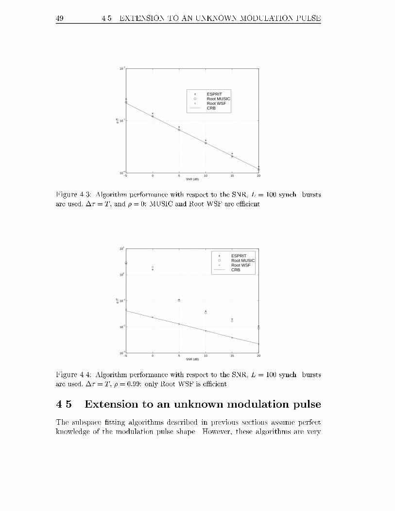
49 4.5. EXTENSION TO AN UNKNOWN MODULATION PULSE
−5 0 5 10 15 2010
−3
10−2
10−1
SNR (dB)
σ /T
ESPRITRoot MUSICRoot WSFCRB
Figure 4.3: Algorithm performance with respect to the SNR, L = 100 synch. bursts
are used, �� = T , and � = 0: MUSIC and Root WSF are e�cient.
−5 0 5 10 15 2010
−3
10−2
10−1
100
101
SNR (dB)
σ /T
ESPRITRoot MUSICRoot WSFCRB
Figure 4.4: Algorithm performance with respect to the SNR, L = 100 synch. bursts
are used, �� = T , � = 0:99: only Root WSF is e�cient.
4.5 Extension to an unknown modulation pulse
The subspace �tting algorithms described in previous sections assume perfect
knowledge of the modulation pulse shape. However, these algorithms are very
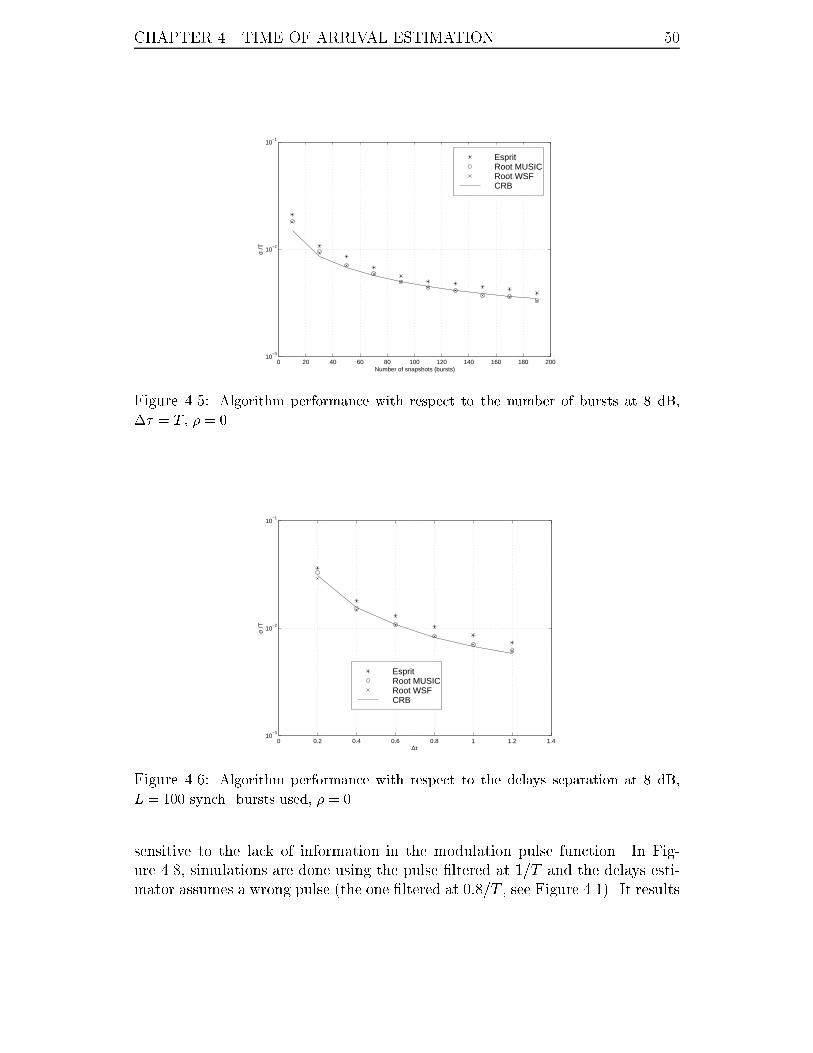
CHAPTER 4. TIME OF ARRIVAL ESTIMATION 50
0 20 40 60 80 100 120 140 160 180 20010
−3
10−2
10−1
Number of snapshots (bursts)
σ /T
EspritRoot MUSICRoot WSFCRB
Figure 4.5: Algorithm performance with respect to the number of bursts at 8 dB,
�� = T , � = 0.
0 0.2 0.4 0.6 0.8 1 1.2 1.410
−3
10−2
10−1
∆τ
σ /T
EspritRoot MUSICRoot WSFCRB
Figure 4.6: Algorithm performance with respect to the delays separation at 8 dB,
L = 100 synch. bursts used, � = 0.
sensitive to the lack of information in the modulation pulse function. In Fig-
ure 4.8, simulations are done using the pulse �ltered at 1=T and the delays esti-
mator assumes a wrong pulse (the one �ltered at 0:8=T , see Figure 4.1). It results
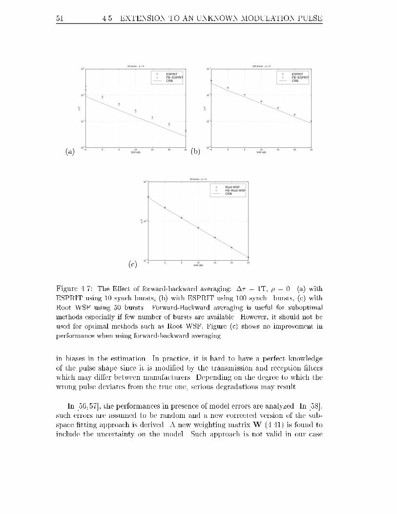
51 4.5. EXTENSION TO AN UNKNOWN MODULATION PULSE
(a) −5 0 5 10 15 20 2510
−3
10−2
10−1
100
10 bursts − ρ = 0
SNR (dB)
σ /T
ESPRITFB−ESPRITCRB
(b) −5 0 5 10 15 20 2510
−4
10−3
10−2
10−1
100 bursts − ρ = 0
SNR (dB)
σ /T
ESPRITFB−ESPRITCRB
(c) −5 0 5 10 15 20 2510
−3
10−2
10−1
50 bursts − ρ = 0
SNR (dB)
σ /T
Root WSFFB−Root WSFCRB
Figure 4.7: The E�ect of forward-backward averaging: �� = 1T, � = 0. (a) with
ESPRIT using 10 synch bursts, (b) with ESPRIT using 100 synch. bursts, (c) with
Root WSF using 50 bursts. Forward-Backward averaging is useful for suboptimal
methods especially if few number of bursts are available. However, it should not be
used for optimal methods such as Root WSF, Figure (c) shows no improvement in
performance when using forward-backward averaging.
in biases in the estimation. In practice, it is hard to have a perfect knowledge
of the pulse shape since it is modi�ed by the transmission and reception �lters
which may di�er between manufacturers. Depending on the degree to which the
wrong pulse deviates from the true one, serious degradations may result.
In [56,57], the performances in presence of model errors are analyzed. In [58],
such errors are assumed to be random and a new corrected version of the sub-
space �tting approach is derived. A new weighting matrix W (4.41) is found to
include the uncertainty on the model. Such approach is not valid in our case
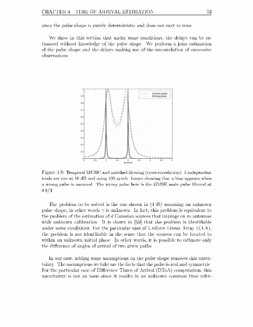
CHAPTER 4. TIME OF ARRIVAL ESTIMATION 52
since the pulse shape is purely deterministic and does not vary in time.
We show in this section that under some conditions, the delays can be es-
timated without knowledge of the pulse shape. We perform a joint estimation
of the pulse shape and the delays making use of the uncorrelation of successive
observations.
0 0.5 1 1.5 2 2.5 3 3.5 40
0.1
0.2
0.3
0.4
0.5
0.6
0.7
0.8
0.9
1
Bit period
Correct pulseWrong pulse
Figure 4.8: Temporal MUSIC and matched �ltering (cross-correlation): 5 independent
trials are run at 10 dB and using 100 synch. bursts showing that a bias appears when
a wrong pulse is assumed. The wrong pulse here is the GMSK main pulse �ltered at
0.8/T.
The problem to be solved is the one shown in (4.45) assuming an unknown
pulse shape, in other words is unknown. In fact, this problem is equivalent to
the problem of the estimation of d Gaussian sources that impinge on m antennae
with unknown calibration. It is shown in [59] that the problem is identi�able
under some conditions. For the particular case of Uniform Linear Array (ULA),
the problem is not identi�able in the sense that the sources can be located to
within an unknown initial phase. In other words, it is possible to estimate only
the di�erence of angles of arrival of two given paths.
In our case, adding some assumptions on the pulse shape removes this uncer-
tainty. The assumptions we take are the facts that the pulse is real and symmetric.
For the particular case of Di�erence Times of Arrival (DToA) computation, this
uncertainty is not an issue since it results in an unknown common time refer-
53 4.5. EXTENSION TO AN UNKNOWN MODULATION PULSE
ence for all times of arrival. This reference will be removed when computing the
di�erences.
4.5.1 Iterative approach
Iterative algorithms have been proposed in the literature, see [42, 43]. These
algorithms jointly estimate the diagonal elements of the matrix �( ) and the
delays � (see equation 4.45). They proposed a general procedure that uses any
algorithm that works assuming known matrix �. It is based on the following
equation that stems from the fact that �( )~A(�) lies in the signal subspace
represented by ~Es, i.e:
[ � ]T= argmax
;�
dXi=1
k ~E�
s�( )~a(�i)k2 (4.64)
This is equivalent to:
[ � ]T= argmax
;� �
dXi=1
D�i~Es~E�
sDi (4.65)
where Di = diag [~a(�i)]. In other words, is the eigenvector associated to the
maximum eigenvalue of the matrixP
d
i=1D�i~Es
~E�
sDi. The proposed algorithm is
similar to the one in [43].
Once this eigenvector is computed, we eliminate the uncertainty on by
incorporating the constraint that the pulse is symmetric and real (i.e. its Fourier
transform is real and symmetrical):
� First of all, the delays are estimated with a standard algorithm assuming
that �( ) is the identity, or using �( ) that corresponds to the original
GMSK pulse.
� is then computed using (4.65) by taking the elements of the eigenvector
associated to the highest eigenvalue VMAX = [v1 � � � vm]:
i =qjvijjvm+1�ij 1 � i � m
� The delays are computed again using found in previous step and so on
until some convergence criterion is achieved.
Note that to obtain an estimation of the pulse shape, should be normalized
so that � = 1.
CHAPTER 4. TIME OF ARRIVAL ESTIMATION 54
4.5.2 A modi�ed ESPRIT algorithm
In the following, a non-iterative ESPRIT-like algorithm is derived in contrast to
the iterative approach described in previous section where the standard ESPRIT
can be used to compute the delays at each iteration. We note D(�) = diag(�)
the diagonal matrix �2��11 , and (�) = T�1�(�)T. Note that � is function of
and represents some unknown vector related to the pulse shape. From equation
(4.61) it appears that the problem to be solved is the following:
[� (�)]T = argmin�
kD(�)J1 ~Es � J2 ~Es(�)k2 (4.66)
with the following constraints:
8<:
Im(�) = 0
JD(�)JD(�) = I(4.67)
These constraints are direct consequences of the assumptions we made on the
pulse shape. In particular, we have:
det[D(�)] = 1 (4.68)
The delays to be estimated are obtained from the phases of the eigenvalues
of since � is diagonal. Es is obtained from the estimated covariance matrix
K~h =1L
PL
j=1~Hj
~H�j.
The solution to the problem shown in (4.66) without incorporation of the
constraints (4.67) is given by [60]:
(�) =
�J2 ~Es
�yD(�)J1 ~Es
Substituting this expression in 4.66, we get:
� = argmin�
Tr
�D(�)J1 ~Es
~E�
sJT1D
�(�)�?J2~Es
�
= argmin�����?J2
~Es� J1( ~Es
~E�
s)TJT1
��
In other words:
� = �VMIN
where VMIN = [v1 � � � vm�1] is the eigenvector of �?J2
~Es� J1( ~Es
~E�
s)TJT1 associ-
ated to the smallest eigenvalue and � a scale factor. The delays estimation are
related to the phases of the eigenvalues of (�) and are then indi�erent to the
magnitude of �. This is a set of solutions determined by an initial phase that is

55 4.5. EXTENSION TO AN UNKNOWN MODULATION PULSE
related to the argument of �.
Adding the constraint that the pulse is real and symmetric forces this so-
lution to be unique. We propose the following solution: � = [�1 � � � �m�1] with�i =
rjvij
jvm�ijso that the constraints shown in (4.67) are satis�ed.
It should be noted that the solution shown here is not optimal since the con-
straints have been applied on the unconstrainted solution.
The pulse can be deduced from � by:
i = �a(fi) =
Qi�1j=1
1�jP
m
k=1
Qk�1j=1
1�2j
1 � i � m (4.69)
where we assumed that �0 = 1.
4.5.3 The DToA special case
As discussed in Section 3.4, the localization procedure makes use of Di�erences
Times of Arrival (DToA). In other words, it computes the di�erences of times of
arrival calculated on several links between the mobile and the base stations.
In that case, the discussion on identi�ability is no more relevant since the
problem is related to the determination of a scale factor of or �. Such a scale
factor introduces a shift to all delays and does not a�ect the di�erences of times
of arrival.
We can generalize the algorithms described above by combining all available
links. The non-iterative approach will be written as:
[�; 1; 2; � � �]T = arg min�;1;2;���
Xi
�ikD(�)J1 ~Esi� J2 ~Esi
ik2 (4.70)
where i is the matrix (�) that correspond to the i-th link, � the column
vector that contains the pulse information that is shared on all links, ~Esithe
estimated signal subspace on the i-th link, and �i a weighting factor; it can be a
function of the signal-to-interference ratio on the i-th link. It is however hard to
set an optimal value to these coe�cients. This problem remains an open question.
The solution is:
~i =
�J2 ~Esi
�yD(�)J1 ~Esi
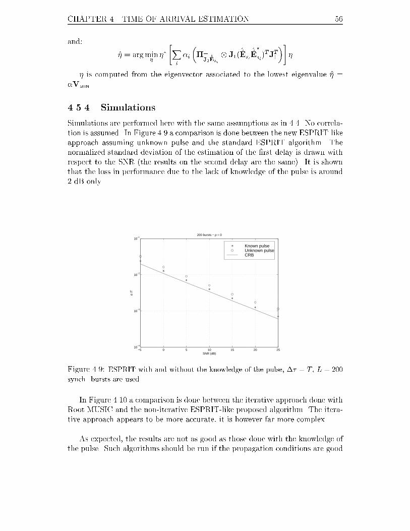
CHAPTER 4. TIME OF ARRIVAL ESTIMATION 56
and:
� = argmin���"X
i
�i
��?J2
~Esi� J1( ~Esi
~E�
si)TJT1
�#�
� is computed from the eigenvector associated to the lowest eigenvalue � =
�VMIN.
4.5.4 Simulations
Simulations are performed here with the same assumptions as in 4.4. No correla-
tion is assumed. In Figure 4.9 a comparison is done between the new ESPRIT-like
approach assuming unknown pulse and the standard ESPRIT algorithm. The
normalized standard deviation of the estimation of the �rst delay is drawn with
respect to the SNR (the results on the second delay are the same). It is shown
that the loss in performance due to the lack of knowledge of the pulse is around
2 dB only.
−5 0 5 10 15 20 2510
−4
10−3
10−2
10−1
200 bursts − ρ = 0
SNR (dB)
σ /T
Known pulseUnknown pulseCRB
Figure 4.9: ESPRIT with and without the knowledge of the pulse, �� = T , L = 200
synch. bursts are used.
In Figure 4.10 a comparison is done between the iterative approach done with
Root MUSIC and the non-iterative ESPRIT-like proposed algorithm. The itera-
tive approach appears to be more accurate, it is however far more complex.
As expected, the results are not as good as those done with the knowledge of
the pulse. Such algorithms should be run if the propagation conditions are good
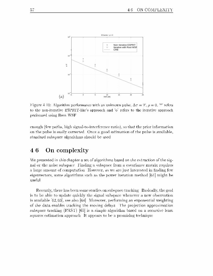
57 4.6. ON COMPLEXITY
(a)−5 0 5 10 15 20 25
10−3
10−2
10−1
100
20 bursts − ρ = 0
SNR (dB)
σ /T
Non−iterative ESPRITIterative with Root WSFCRB
Figure 4.10: Algorithm performance with an unknown pulse, �� = T , � = 0, '*' refers
to the non-iterative ESPRIT-like's approach and 'o' refers to the iterative approach
performed using Root WSF.
enough (few paths, high signal-to-interference ratio), so that the prior information
on the pulse is easily corrected. Once a good estimation of the pulse is available,
standard subspace algorithms should be used.
4.6 On complexity
We presented in this chapter a set of algorithms based on the extraction of the sig-
nal or the noise subspace. Finding a subspace from a covariance matrix requires
a large amount of computation. However, as we are just interested in �nding few
eigenvectors, some algorithms such as the power iteration method [61] might be
useful.
Recently, there has been some studies on subspace tracking. Basically, the goal
is to be able to update quickly the signal subspace whenever a new observation
is available [62,63], see also [64]. Moreover, performing an exponential weighting
of the data enables tracking the moving delays. The projection approximation
subspace tracking (PAST) [65] is a simple algorithm based on a recursive least
squares estimation approach. It appears to be a promising technique.

CHAPTER 4. TIME OF ARRIVAL ESTIMATION 58
Chapter 5
Hyperbolic trilateration
In this chapter, we deal with the problem of estimating the coordinates of the
handset once enough times of arrival are available. This procedure called trilat-
eration or data fusion is possible if information on the network synchronization
is available. The problem reduced then to a non linear maximization.
5.1 Problem statement
We have n times of arrival observations and m di�erences of synchronization ob-
servations. All these observations are corrupted with noise.
The times of arrival can be written in the following way:
fi =ri
c+ ti � q1 + bi 1 � i � n (5.1)
with,
� ri the distance between the mobile and the i-th base station,
� c � 3:108 m/s the speed of light,
� ti the transmission time of the i-th transmitter,
� q1 a reference time1,
� fi the estimated times of arrival,
� bi an additive white Gaussian noise.
1It should be noted that this reference has a di�erent interpretation according to the location
system. For instance in the GPS system [66] this will be the handset reference.
59
CHAPTER 5. HYPERBOLIC TRILATERATION 60
The n base stations involved in the localization procedure are assumed to
have di�erent coordinates. Indeed the mobile can hear more cells that sites (in
the case of trisectorized sites for instance) and the cells that belong to the same
base station provide little extra information.
The synchronization information is expressed by the following n equations:
�ti = ti � q2 + wi 1 � i � n (5.2)
Such measurements can be simply computed by measuring the times of arrival
of di�erent signals coming from di�erent base stations to a known point as will
be discussed in next chapter. q2 is another reference time, and wi an additive
white Gaussian noise.
We can rewrite these equations in a more compact way:
(~F = A(�) +T� q11+Bf
�T = T� q21+Bt
(5.3)
with,
� � the column vector of the coordinates to be estimated (in two dimensions
� = [x y]T ),
� ~F = [f1 � � � fn]T ,
� A(�) = 1c[r1 � � � rn]T ,
� T = [t1 � � � tn]T ,
� Bf = [b1 � � � bn]T ,
� Bt = [w1 � � �wm]T ,
� 1 = [1 � � �1]T .
We assume that the noise vectors Bf and Bt are zero mean Gaussian variables
with the following covariances:
� E[BfBT
f] = Qf
� E[BtBT
t] = Qt
� E[BfBT
t] = 0

61 5.1. PROBLEM STATEMENT
Let Q = Qt + Qf . This covariance matrix contains the con�dence values
of the time of arrival measurements after incorporation of the synchronization
information uncertainties.
Obviously the system (5.3) is equivalent to:
~F = A(�) + �T� tr1+B
where B = Bf + Bt and tr = q1 + q2. Incorporating �T in ~F the system
becomes:
F = A(�)� tr1+B (5.4)
where F = ~F � �T. These equation leads to a hyperbolic trilateration as in
GPS [66]. n must be strictly greater than two if the position estimation is re-
quired in two dimensions since three variables need to be estimated: x, y, and tr.
This is required for the system to be identi�able, but of course, the greater is n,
the better is the accuracy. In the speci�c case of radio propagation, it should be
noted that the times of arrival (i.e. ~F) are biased in general because of multipath
propagation. For instance, the direct line of sight may not exist at all.
We perform a joint estimation of � and tr. From (5.4) the maximum likelihood
estimator is given by:
[� tr] = argmax�;tr
[F�A(�)� tr1]TQ�1 [F�A(�)� tr1] (5.5)
Derivating with respect to tr, we obtain:
tr(�) =1TQ�1 [F�A(�)]
1TQ�11(5.6)
Substituting in (5.5), we obtain a concentrate function to be minimized with
respect to �:
� = argmax�
[F�A(�)]T ~Q [F�A(�)] (5.7)
with:
~Q = Q�1 � Q�111TQ�1
1TQ�11
Note that ~Q is rank de�cient since ~Q1 = 0. That is the reason why the time
reference has been eliminated in (5.7) compared to (5.5).
CHAPTER 5. HYPERBOLIC TRILATERATION 62
5.2 Cramer-Rao bound
The Cramer-Rao bound on � is given by (see de�nition in Section 4.2.4):
CRB�1(�) =
"@A(�)
@�
#T~Q@A(�)
@�(5.8)
Proof in Appendix C. In two dimensions we have:
@A(�)
@�=
1
c
2666664
x�x1r1
y�y1r1
x�x2r2
y�y2r2
......
x�xnrn
y�ynrn
3777775 (5.9)
where xi and yi are the coordinates of the i-th transmitter. Therefore the
root mean square of any given estimator is bounded by:
RMS(�) �qTr(CRB(�))
This bound is clearly � dependent. This fact is important and means that
the performance of the estimator depends on the problem geometry. This phe-
nomenon is called Geometric Dilution of Precision (GDoP); it indicates how much
the geometry in uences the �nal location error [67].
In simulations, we will take a mean value for the RMS:
RMS �
vuutRS Tr [CRB(�)] d�RS d�
(5.10)
In the GSM standard, an additional interesting piece of data is available: the
timing advance (see Section 2.3.2). It is an approximation of the propagation
time between the mobile and the base station it is connected to. Taking this
information into account the trilateration is the intersection of hyperbolas with a
circle centered on the base station and with a radius equal to the timing advance
parameter expressed in meters. For simplicity we will take the base station the
mobile is connected to as a reference so that the timing advance can be written
as:
TA = j�j+ bTA
bTA refers to the perturbation on the timing advance, we will assume it as being
Gaussian with zero mean and variance �TA. We will noteCRBTA the Cramer-Rao
bound taking into account this new information. Using the formula: @j�j@�
= �
j�j ,
the new Fisher information matrix is:
FIMTA(�) = FIM(�) +1
�2TA
��T
j�j2 (5.11)
63 5.3. ALGORITHMS FOR HYPERBOLIC TRILATERATION
The inverse matrix lemma yields:
CRBTA(�) = CRB(�)
"I� ��TCRB(�)
�2TAj�j2 + �TCRB(�)�
#(5.12)
It is interesting to note two special cases:
� �2TA! 1, i.e. no information available on the timing advance, obviously
implies
CRBTA(�)! CRB(�)
� �2TA! 0, i.e. exact knowledge of the timing advance, implies
CRBTA(�)! CRB(�)
"I� ��TCRB(�)
�TCRB(�)�
#
5.3 Algorithms for hyperbolic trilateration
5.3.1 Taylor expansion (scoring method)
This is an iterative algorithm for directly minimizing the maximum likelihood
criterion (5.7) by performing a Taylor expansion of A(�):
A(�n) � A(�n�1) +@A(�n�1)
@�[�n � �n�1] (5.13)
Replacing this equation in (5.7) gives:
�n = argmax�
"F�A(�n�1)�
@A(�n�1)
@�(� � �n�1)
#T~Q (5.14)
"F�A(�n�1)�
@A(�n�1)
@�(� � �n�1)
#
And each iteration will be written as follows [68]:
�n = �n�1 +
24 @A(�n�1)
@�
!T
~Q@A(�n�1)
@�
35�1
@A(�n�1)
@�
!T
~Q [F�A(�n�1)]
(5.15)
The algorithm converges to the value that minimizes the log-likelihood when-
ever a proper initialization is available. This algorithm is also called the scoring
method: it is the Newton-Raphson method [69] in which the Hessian has been
replaced by its expected value. This expected value is nothing but the Fisher
information matrix. Note that this matrix has the same dimension of � (two or
three) and is therefore very simple to invert. Note also that the base stations
must not be arranged linearly so that the Fisher Information Matrix is full column
rank.
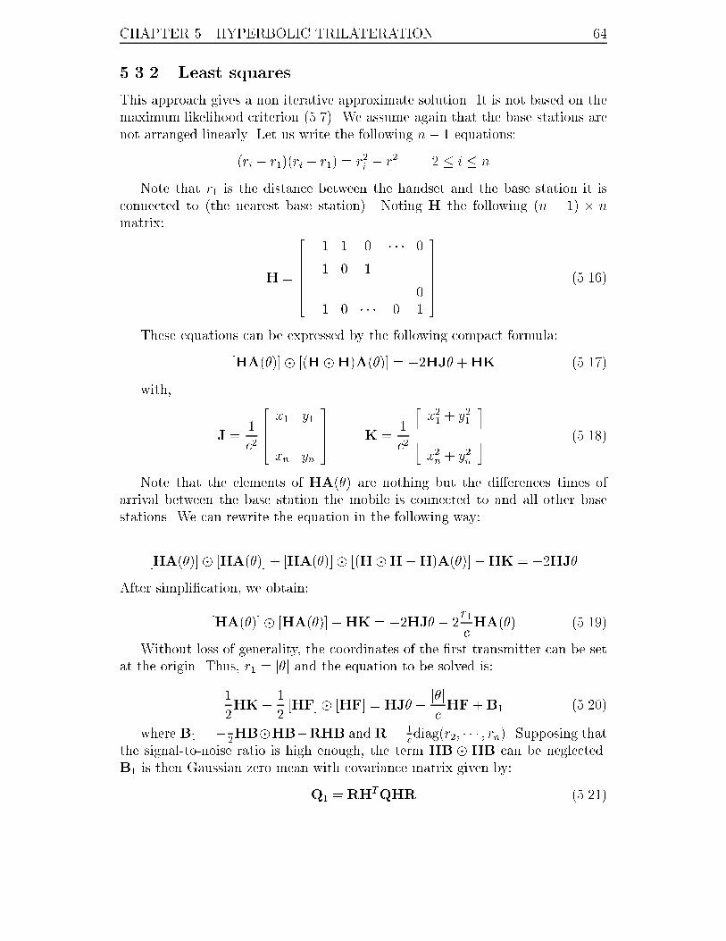
CHAPTER 5. HYPERBOLIC TRILATERATION 64
5.3.2 Least squares
This approach gives a non iterative approximate solution. It is not based on the
maximum likelihood criterion (5.7). We assume again that the base stations are
not arranged linearly. Let us write the following n� 1 equations:
(ri � r1)(ri + r1) = r2i� r21 2 � i � n
Note that r1 is the distance between the handset and the base station it is
connected to (the nearest base station). Noting H the following (n � 1) � n
matrix:
H =
2666664
�1 1 0 � � � 0
�1 0 1. . .
......
.... . .
. . . 0
�1 0 � � � 0 1
3777775 (5.16)
These equations can be expressed by the following compact formula:
[HA(�)]� [(H�H)A(�)] = �2HJ� +HK (5.17)
with,
J =1
c2
2664x1 y1...
...
xn yn
3775 K =
1
c2
2664x21 + y21
...
x2n+ y2
n
3775 (5.18)
Note that the elements of HA(�) are nothing but the di�erences times of
arrival between the base station the mobile is connected to and all other base
stations. We can rewrite the equation in the following way:
[HA(�)]� [HA(�)] + [HA(�)]� [(H�H�H)A(�)]�HK = �2HJ�
After simpli�cation, we obtain:
[HA(�)]� [HA(�)]�HK = �2HJ� � 2r1
cHA(�) (5.19)
Without loss of generality, the coordinates of the �rst transmitter can be set
at the origin. Thus, r1 = j�j and the equation to be solved is:
1
2HK� 1
2[HF]� [HF] = HJ� +
j�jcHF +B1 (5.20)
where B1 = �12HB�HB�RHB and R = 1
cdiag(r2; � � � ; rn). Supposing that
the signal-to-noise ratio is high enough, the term HB � HB can be neglected.
B1 is then Gaussian zero mean with covariance matrix given by:
Q1 = RHTQHR (5.21)
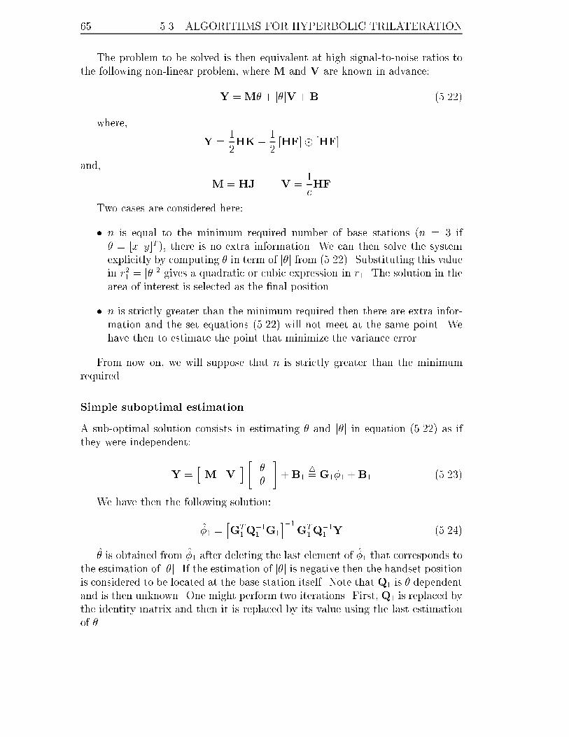
65 5.3. ALGORITHMS FOR HYPERBOLIC TRILATERATION
The problem to be solved is then equivalent at high signal-to-noise ratios to
the following non-linear problem, where M and V are known in advance:
Y =M� + j�jV +B1 (5.22)
where,
Y =1
2HK� 1
2[HF]� [HF]
and,
M = HJ V =1
cHF
Two cases are considered here:
� n is equal to the minimum required number of base stations (n = 3 if
� = [x y]T ), there is no extra information. We can then solve the system
explicitly by computing � in term of j�j from (5.22). Substituting this value
in r21 = j�j2 gives a quadratic or cubic expression in r1. The solution in the
area of interest is selected as the �nal position.
� n is strictly greater than the minimum required then there are extra infor-
mation and the set equations (5.22) will not meet at the same point. We
have then to estimate the point that minimize the variance error.
From now on, we will suppose that n is strictly greater than the minimum
required.
Simple suboptimal estimation
A sub-optimal solution consists in estimating � and j�j in equation (5.22) as if
they were independent:
Y =hM V
i " �
j�j
#+B1
4= G1�1 +B1 (5.23)
We have then the following solution:
�1 =hGT
1Q�11 G1
i�1GT
1Q�11 Y (5.24)
� is obtained from �1 after deleting the last element of �1 that corresponds to
the estimation of j�j. If the estimation of j�j is negative then the handset positionis considered to be located at the base station itself. Note that Q1 is � dependent
and is then unknown. One might perform two iterations. First, Q1 is replaced by
the identity matrix and then it is replaced by its value using the last estimation
of �.
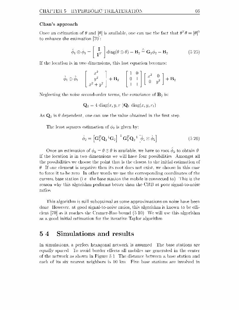
CHAPTER 5. HYPERBOLIC TRILATERATION 66
Chan's approach
Once an estimation of � and j�j is available, one can use the fact that �T � = j�j2to enhance the estimation [70]:
�1 � �1 =
"I
1T
#diag(� � �) +B2
4= G2�2 +B2 (5.25)
If the location is in two dimensions, this last equation becomes:
�1 � �1 =
264
x2
y2
x2 + y2
375 +B2 =
2641 0
0 1
1 1
375"x2 0
0 y2
#+B2
Neglecting the noise second-order terms, the covariance of B2 is:
Q2 = 4 diag(x; y; r1)Q1 diag(x; y; r1)
As Q2 is � dependent, one can use the value obtained in the �rst step.
The least squares estimation of �2 is given by:
�2 =hGT
2Q�12 G2
i�1GT
2Q�12
h�1 � �1
i(5.26)
Once an estimation of �2 = �� � is available, we have to root �2 to obtain �.If the location is in two dimensions we will have four possibilities. Amongst all
the possibilities we choose the point that is the closest to the initial estimation of
�. If one element is negative then its root does not exist, we choose in this case
to force it to be zero. In other words we use the corresponding coordinates of the
current base station (i.e. the base station the mobile is connected to). This is the
reason why this algorithm performs better than the CRB at poor signal-to-noise
ratios.
This algorithm is still suboptimal as some approximations on noise have been
done. However, at good signal-to-noise ratios, this algorithm is known to be e�-
cient [70] as it reaches the Cramer-Rao bound (5.10). We will use this algorithm
as a good initial estimation for the iterative Taylor algorithm.
5.4 Simulations and results
In simulations, a perfect hexagonal network is assumed. The base stations are
equally spaced. To avoid border e�ects all mobiles are generated in the center
of the network as shown in Figure 5.1. The distance between a base station and
each of its six nearest neighbors is 10 km. Five base stations are involved in
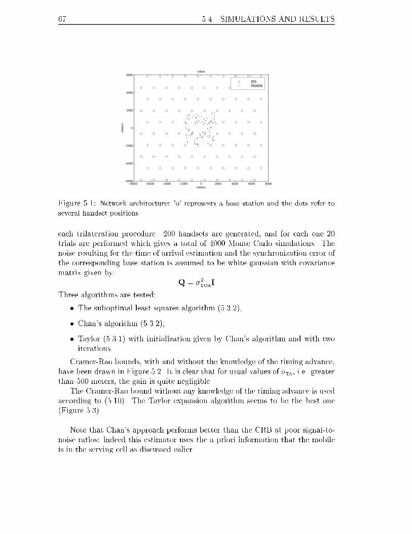
67 5.4. SIMULATIONS AND RESULTS
−8000 −6000 −4000 −2000 0 2000 4000 6000 8000−6000
−4000
−2000
0
2000
4000
6000
meters
met
ers
urban
BSMobile
Figure 5.1: Network architecture: 'o' represents a base station and the dots refer to
several handset positions.
each trilateration procedure. 200 handsets are generated, and for each one 20
trials are performed which gives a total of 4000 Monte Carlo simulations. The
noise resulting for the time of arrival estimation and the synchronization error of
the corresponding base station is assumed to be white gaussian with covariance
matrix given by:
Q = �2TOA
I
Three algorithms are tested:
� The suboptimal least squares algorithm (5.3.2),
� Chan's algorithm (5.3.2),
� Taylor (5.3.1) with initialization given by Chan's algorithm and with two
iterations.
Cramer-Rao bounds, with and without the knowledge of the timing advance,
have been drawn in Figure 5.2. It is clear that for usual values of �TA, i.e. greater
than 500 meters, the gain is quite negligible.
The Cramer-Rao bound without any knowledge of the timing advance is used
according to (5.10). The Taylor expansion algorithm seems to be the best one
(Figure 5.3).
Note that Chan's approach performs better than the CRB at poor signal-to-
noise ratios: indeed this estimator uses the a priori information that the mobile
is in the serving cell as discussed ealier.
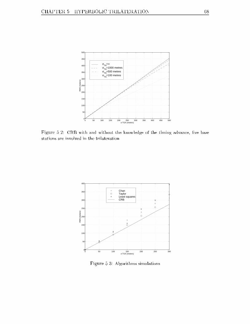
CHAPTER 5. HYPERBOLIC TRILATERATION 68
0 50 100 150 200 250 300 350 400 450 5000
50
100
150
200
250
300
350
400
450
500
σ TOA (meters)
RM
S (
met
ers)
σTA
=∞σ
TA=1000 metres
σTA
=500 metresσ
TA=100 metres
Figure 5.2: CRB with and without the knowledge of the timing advance, �ve base
stations are involved in the trilateration.
0 50 100 150 200 250 3000
50
100
150
200
250
300
350
400
σ TOA (meters)
RM
S (
met
ers)
ChanTaylorLeast squaresCRB
Figure 5.3: Algorithms simulations
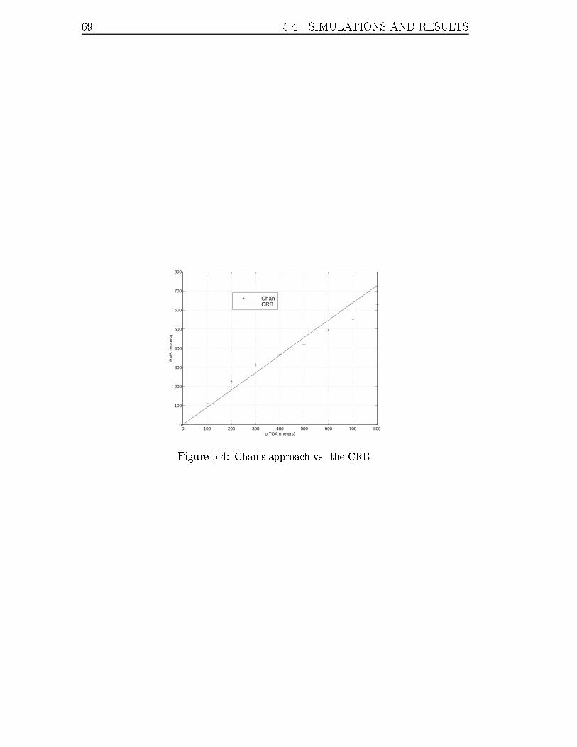
69 5.4. SIMULATIONS AND RESULTS
0 100 200 300 400 500 600 700 8000
100
200
300
400
500
600
700
800
σ TOA (meters)
RM
S (
met
ers)
ChanCRB
Figure 5.4: Chan's approach vs. the CRB.

CHAPTER 5. HYPERBOLIC TRILATERATION 70
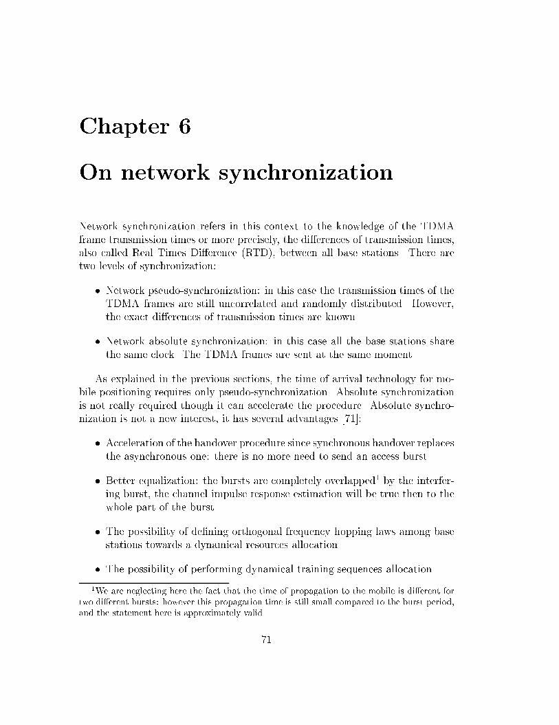
Chapter 6
On network synchronization
Network synchronization refers in this context to the knowledge of the TDMA
frame transmission times or more precisely, the di�erences of transmission times,
also called Real Times Di�erence (RTD), between all base stations. There are
two levels of synchronization:
� Network pseudo-synchronization: in this case the transmission times of the
TDMA frames are still uncorrelated and randomly distributed. However,
the exact di�erences of transmission times are known.
� Network absolute synchronization: in this case all the base stations share
the same clock. The TDMA frames are sent at the same moment.
As explained in the previous sections, the time of arrival technology for mo-
bile positioning requires only pseudo-synchronization. Absolute synchronization
is not really required though it can accelerate the procedure. Absolute synchro-
nization is not a new interest, it has several advantages [71]:
� Acceleration of the handover procedure since synchronous handover replaces
the asynchronous one: there is no more need to send an access burst.
� Better equalization: the bursts are completely overlapped1 by the interfer-
ing burst, the channel impulse response estimation will be true then to the
whole part of the burst.
� The possibility of de�ning orthogonal frequency hopping laws among base
stations towards a dynamical resources allocation.
� The possibility of performing dynamical training sequences allocation.
1We are neglecting here the fact that the time of propagation to the mobile is di�erent for
two di�erent bursts: however this propagation time is still small compared to the burst period,
and the statement here is approximately valid.
71
CHAPTER 6. ON NETWORK SYNCHRONIZATION 72
Note that to get these advantages, a synchronization error below one bit pe-
riod is enough. However, this is not enough for location purposes since one bit
period is equivalent to 1108 meters of propagation. Moreover it is hard to main-
tain this degree of synchronization since the base stations keep drifting randomly
due to the di�erences of their local oscillatories. For these reasons, we prefer the
pseudo-synchronization scenario.
The basic idea to get the synchronization information is in the exploitation
of the location information; to get the handset position, synchronization infor-
mation is required, so if the position is known in advance then it is easy to get
the synchronization information. In other words, dedicated mobiles (also called
LMU for Location Mobile Unit) can be used successfully at known positions to
get the synchronization information. This information can be reported periodi-
cally (one report per minute). Assuming that the base stations drift slowly, it is
possible to interpolate between two consecutive reports. In fact, there are some
requirements on base station drifts; they are not allowed to exceed 50 ns/s.
Of course the use of an external device such as the GPS system to get the
synchronization information is possible but it is not the subject of this dissertation
since we are concerned with a system where the network locates its subscribers
by its own capability.
6.1 The pseudo-synchronization problem
As shown in Figure 6.1, the pseudo-synchronization problem may be de�ned as
to estimate the di�erences in TDMA transmission times according to a set of
observations of these di�erences. If we refer to each real times di�erence obser-
vation by a connection that links the two concerned base stations, we can then
de�ne a graph composed from the base stations and these links. The pseudo-
synchronization problem is identi�able if and only if the graph is connected, in
other words all base stations must be connected with at least one link.
The m real times di�erence noisy observations are put into one single column
vector Y:
Y =MX+B (6.1)
X is a vector with dimension equal to the number of observed links in the
network a. The number of unobserved links is then n(n�1)2
� a. B is a Gaussian
noise with zero mean and covariance Q. Note that M is full column rank. Some
RTDs might be measured more than one time. The unknown RTDs are computed
by taking into account the constraint that the sum on any cycle in the graph is null
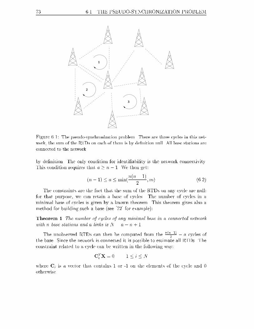
73 6.1. THE PSEUDO-SYNCHRONIZATION PROBLEM
1
2
3
Figure 6.1: The pseudo-synchronization problem. There are three cycles in this net-
work, the sum of the RTDs on each of them is by de�nition null. All base stations are
connected to the network.
by de�nition. The only condition for identi�ability is the network connectivity.
This condition requires that a � n� 1. We then get:
(n� 1) � a � min(n(n� 1)
2; m) (6.2)
The constraints are the fact that the sum of the RTDs on any cycle are null:
for that purpose, we can retain a base of cycles. The number of cycles in a
minimal base of cycles is given by a known theorem. This theorem gives also a
method for building such a base (see [72] for example):
Theorem 1 The number of cycles of any minimal base in a connected network
with n base stations and a links is N = a� n + 1.
The unobserved RTDs can then be computed from then(n�1)
2� a cycles of
the base. Since the network is connected it is possible to estimate all RTDs. The
constraint related to a cycle can be written in the following way:
CT
iX = 0 1 � i � N
where Ci is a vector that contains 1 or -1 on the elements of the cycle and 0
otherwise.

CHAPTER 6. ON NETWORK SYNCHRONIZATION 74
The system to be solved is a least squares problem with constraints:
(Y =MX+B
CTX = 0(6.3)
where C = [C1 � � �CN ] is full column rank (independent cycles).
This system can be easily solved using Lagrange multipliers:
J(X) =1
2[Y �MX]
TQ�1 [Y �MX] + �TCTX (6.4)
Derivating J with respect to X will give:
@J(X)
@X= �MTQ�1 [Y �MX] +C� (6.5)
We note ~X =hMTQ�1M
i�1MTQ�1Y the weighted least squares estimation
of the RTDs from the observations without any constraint, andK =hMTQ�1M
i�1its error covariance.
Setting the derivative with respect to X to zero, we get the following:
� =�CTKC
��1CT ~X
The �nal solution can be expressed in the following way:
X =
�I�KC
�CTKC
��1CT
�~X (6.6)
The interpretation is simple. It is a weighted projection matrix. Supposing
the noise is white and that each RTD is observed once, i.e. K = �2I, equation
(6.6) becomes:
X = �?C~X (6.7)
Incorporating a constraint is equivalent to project the estimated RTDs (with-
out constraints) onto the null space of C. In the case the cycles do not share
any element, i.e. CT
iCj = CT
iCi�ij, equation (6.7) consists in removing the mean
RTD in a cycle from each of its element.
Simple algebra manipulations show that:
X = X+
�I�KC
�CTKC
��1CT
�KMTQ�1B (6.8)
75 6.2. ABSOLUTE SYNCHRONIZATION
This proves that our estimator is unbiased with covariance matrix given by:
KX=
�I�KC
�CTKC
��1CT
�K
Again, if K = �2I, then we simply have KX= �2�T
C. In other words, the noise
variance is reduced by:
Tr(�T
C)
Tr(Q)=a�N
a=n� 1
a(6.9)
Taking into account relation (6.2) the gain is somewhere between 1 and 2n. If
we suppose that L realizations ofY are available, then we can use the same results
substitutingY with 1L
PL
i=1Yi. The resulting noise variance will be reduced by L.
It is possible to extend the algorithm in presence of drifts. If we suppose that
the base stations are drifting slowly with di�erent speeds, we can use a Kalman
�lter to estimate jointly drift and o�set of each base station. Xi must then be
estimated from the following system:
8><>:Yi =MXi +Bi
Xi = Xi�1 +MV�t+Wi
CTXi = 0
(6.10)
where V is a vector that contains the drift di�erences, and �t the period
between two consecutive measurements.
6.2 Absolute synchronization
This approach is di�erent from previous one in the sense that each base station
corrects iteratively its time o�set until a global synchronized state is reached.
Each correction is made by monitoring the neighboring base stations. The al-
gorithm is iterative since the base stations are not allowed to modify their time
o�set abruptly more than a certain limit. The algorithm presented in the follow-
ing insures an autonomous synchronization; the time o�set corrections are not
centralized but each base station correct its time o�set independently.
Before presenting the algorithm, we introduce the Perron-Frobenius theorem.
De�nition 1 A square matrix A is said to be reducible if and only if the linear
operator de�ned by A contains an invariant subspace. If such a condition is not
veri�ed, the matrix is said to be irreducible.
CHAPTER 6. ON NETWORK SYNCHRONIZATION 76
A reducible matrix A can be written via some permutations under the following
way:
A0 =
0B@B 0
C D
1CA (6.11)
where B and D are two square matrices.
The following theorem is a simpli�ed version of the Perron-Frobenius theorem
[73, 74]:
Theorem 2 If all elements aij of an irreducible matrix A are non negative then
it has one simple real strictly positive maximal eigenvalue r. Noting si =P
n
k=1 aikthe sum of the elements in each row, then:
min1�i�n
si � r � max1�i�n
si (6.12)
Moreover all eigenvalues lies in the disk jzj � max1�i�n si.
The bounds shown in this version of the theorem are not the best achievable
bounds. Nevertheless, they will be enough for our purposes.
The problem to be solved is to synchronize a set of transmitters fAig0�i�N�1.The exact positions of all transmitters are known. We note ti the time o�set of
the i-th transmitter. We suppose that at the beginning, ti is a random variable
uniformly distributed on [0; 1]. For the problem to be identi�able, the network
must be connected. We a�ect to each point in the network a reference time2.
All transmitters are listening to theirs own neighbors. All transmitters have
at least one neighbor since the network is non-oriented and connected. At each
iteration, the time o�set of the i-th transmitter is modi�ed as [75]:
t(n+1)i = t
(n)i + �
PN
j=1 pij(t(n)j � t
(n)i )P
N
j=1 pij(6.13)
pij is a weighting coe�cient, it is a con�dence value that evaluates the link
between the i-th and j-th transmitters. Note that pii = 0. � is a constant that
�xes the convergence speed of the algorithm, 0 < � � �0 < 1 (�0 is the drift
limitation). We are not considering the noise here. Indeed, since the algorithm
requires a high number of successive observations, we assume that the resulting
noise variance converges to zero.
2This assumes that the absolute reference 0 is known and shared by all transmitters. We
can avoid such assumption if the network is roughly synchronized. For example, all TDMA
frames are synchronized to within a multi-frame.
77 6.2. ABSOLUTE SYNCHRONIZATION
Noting Xn = [t1 � � � tN ]T the state of the network at step n and P the matrix
made frompijPN
j=1pij
, we have:
Xn = Xn�1 + �(P� I)Xn�1 = [(1� �)I+ �P]Xn�1 =MXn�1 (6.14)
which �nally gives,
Xn =MnX0 (6.15)
Note that P is not necessarily symmetric since all base stations have not the
same number of neighbors.
Theorem 3 The algorithm described by equation (6.15) always converges in
probability to the synchronized state, in other words:
limn!1
Mnv = �1
where v is a randomly initialized vector and � a scale factor.
Proof 1 It is straightforward to see that P is an irreducible matrix since the
network is assumed to be connected. And since all its element are positive, the
Perron-Frobenius theorem states that the maximal eigenvalue of P is unique and
real. Since the sums of the elements of all rows in P are all equal to one, it
follows that this maximal eigenvalue is one. The eigenvector associated to this
eigenvalue is 1pn1. All other eigenvalues have a module that is less or equal to
1. The eigenvalues of M follows from those of P. All these eigenvalues except
the maximum one that is equal to one are inside the disk jzj < 1. The algorithm
converges then in probability to the synchronized state whatever the initial state
is.
The convergence speed of this algorithm is proportional to the ratio between
the two consecutive strongest eigenvalues, 1�(�)
, where:
�(�) = max1�i�n
(j1� �+ ��ij < 1)
�i refers to the eigenvalues of P. � must be chosen properly to minimize �(�):
� = min
�argmin
��(�); �0
�
�0 is the drift limitation previously de�ned and it is most likely that it is the
fundamental limitation since its value is very low (50 ns/s).
In Figure 6.2, simulations are done in a network consisting of �fty base sta-
tions. We suppose that each base station is connected to the same number of
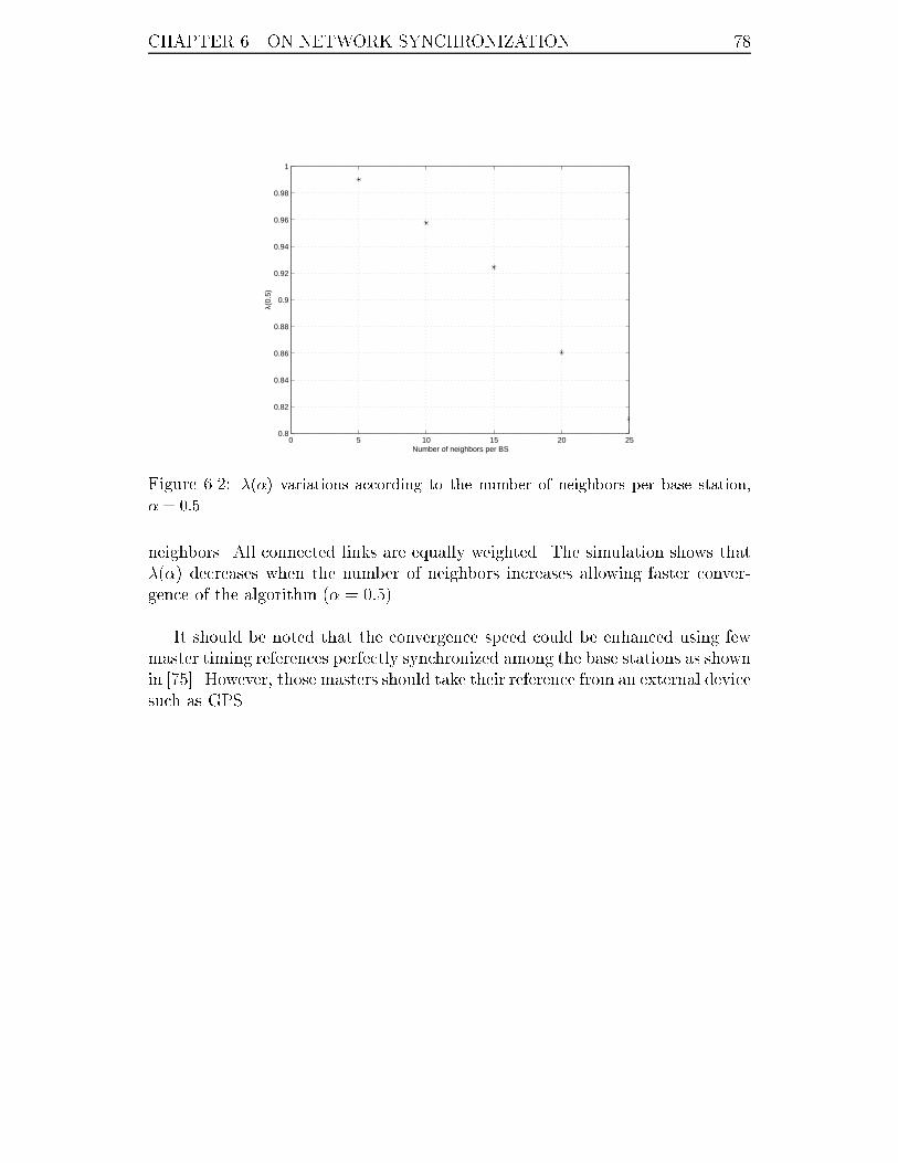
CHAPTER 6. ON NETWORK SYNCHRONIZATION 78
0 5 10 15 20 250.8
0.82
0.84
0.86
0.88
0.9
0.92
0.94
0.96
0.98
1
Number of neighbors per BS
λ(0.
5)
Figure 6.2: �(�) variations according to the number of neighbors per base station,
� = 0:5.
neighbors. All connected links are equally weighted. The simulation shows that
�(�) decreases when the number of neighbors increases allowing faster conver-
gence of the algorithm (� = 0:5).
It should be noted that the convergence speed could be enhanced using few
master timing references perfectly synchronized among the base stations as shown
in [75]. However, those masters should take their reference from an external device
such as GPS.
Chapter 7
Global simulations and �nal
results
In previous sections, simulations were performed independently on time of arrival
estimation and on the trilateration procedure. In this chapter, we combine both
procedures to perform the complete simulation process of a mobile localization.
The performance highly depends on the pro�le of the environment the mobile
is located in. This pro�le determines the parameters related to the channel
impulse response such as the number of paths, the delay spread, or the existence
of the line of sight path. It also determines the path loss that gives the signal-
to-interference ratio.
7.1 Channel impulse response model
In this section, we investigate the way of generating a channel impulse response
represented by a delay spread, a number of paths, and for each one, its time
delay, its mean power, and its amplitude probability distribution.
It is common to say that each path in a channel impulse response is the result
of the superposition of a large number of partial waves, each with a delay time
that corresponds to the delay of this path [76,77]. The amplitude of a given path
is in consequence that of the resulting sum of these partial waves:
E(t) =nXi=1
Ei exp
�j(�0 +
2�
�vt cos�i)
�(7.1)
�i refers to the angle of incidence of the i-th partial wave and �0 the initial
phase. v refers to the mobile velocity.
79
CHAPTER 7. GLOBAL SIMULATIONS AND FINAL RESULTS 80
In the case the path does not correspond to the direct line of sight path, these
partial waves are uncorrelated and have a phase uniformly distributed. The re-
sulting amplitude is Gaussian complex with zero mean, its envelope follows a
Rayleigh distribution. If a strong constant amplitude is present as in the case
of the line of sight path, the resulting amplitude has a non-zero mean, and the
distribution of the envelope is more likely to be Ricean.
The amplitude time correlation function is shown to be (see [77] for example):
R(�) =
Z 2�
0p(�) exp
�j2�
�v� cos�
�d� (7.2)
p(�) refers to the angular distribution of the partial waves. Usually p(�) is
assumed to be uniformly distributed; this assumption leads to the well-known
Jakes' model:
R(�) = J0(2�
�v�) , �R(f) =
1r1�
�f
fd
�2 (7.3)
where �R(f) refers to the Doppler spectrum and fd =v
�refers to the Doppler
frequency. In our simulations, we will assume that p(�) is Gaussian with a con-
stant mean value generated randomly and a standard deviation of 0.15 radians.
This model corresponds to the case where the partial waves are concentrated in a
narrow beam. In general, the higher the velocity is, the less correlated the fading
is.
The fading simulation is done by generating the partial waves randomly ac-
cording to (7.1). If the path is assumed to be purely di�used, i.e. no determin-
istic components present, then all amplitudes are randomly generated and the
resulting amplitude follows a Rayleigh distribution. In contrast, if a strong main
component is present, then the fading is more likely to be Ricean; we therefore
need to select one partial wave among the n to have a stronger amplitude. It is
common to use the Nakagami distribution [78] to model the fading behaviour:
p(r) =2mmr2m�1
�(m)mexp(�m
r2) (7.4)
The constant m is related to the importance of the main component: the
larger is m, the more important is this component. refers to the path energy.
We have three possibilities (see Figure 7.1):
� m = 1: we simply have the Rayleigh distribution.
� m > 1: this is an approximation of the Ricean distribution though it is not
exactly that Ricean distribution (see [79]).
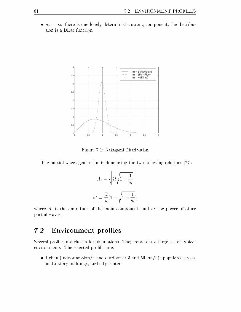
81 7.2. ENVIRONMENT PROFILES
� m = 1: there is one lonely deterministic strong component, the distribu-
tion is a Dirac function.
0 0.5 1 1.5 2 2.5 30
0.5
1
1.5
2
2.5
3
3.5
4
m = 1 (Rayleigh)m = 15 (≈ Rice)m = ∞ (Dirac)
Figure 7.1: Nakagami Distribution
The partial waves generation is done using the two following relations [77]:
A1 =
vuut
s1� 1
m
�2 =
n(1�
s1� 1
m)
where A1 is the amplitude of the main component, and �2 the power of other
partial waves.
7.2 Environment pro�les
Several pro�les are chosen for simulations. They represent a large set of typical
environments. The selected pro�les are:
� Urban (indoor at 3km/h and outdoor at 3 and 50 km/h): populated areas,
multi-story buildings, and city centers.

CHAPTER 7. GLOBAL SIMULATIONS AND FINAL RESULTS 82
� Suburban outdoor (at 3 and 50 km/h): residential houses, suburbs, and
villages.
� Rural outdoor (at 3 and 100 km/h): inhabited areas, highways, �elds, and
forests.
The main di�erence between urban and other pro�les is in the presence of
line of sight path. No line of sight is assumed in the urban whereas a strong
line of sight path is present in the rural and suburban pro�les. Moreover, the
number of scatterers is higher in the urban pro�le and the delay spread is also
longer. These facts lead unavoidably to poorer results in the urban case. The
assumptions made on each of these pro�les are based on the common channel
model that had been established in T1P1.5 meetings [80] for each company to
simulate its own location algorithm.
7.3 Time of Arrival simulations
7.3.1 Assumptions
We are concerned in this section with the channel impulse response model as-
sumptions.
Delay-Spread model
We take the Greenstein model previously discussed (2.7) and set the three pa-
rameters of this model �y, T1, and � according to each pro�le.
Fading model
We use the Nakagami fading model according to the description made in (7.1).
The distribution of the angles of incidence of the partial waves is supposed to be
Gaussian with an initial phase randomly generated and a standard deviation of
0.15 radians.
The power generation is exponential for the urban pro�le; the power of each
delay is weighted with exp(�6�i) where �i is generated uniformly on [0; 1].
Once the powers and delays are generated, powers are normalized so that
their sum is equal to one and the delays are adjusted so that the desired delay
spread (generated according to the Greenstein model) is met:
ai (aiPd
i=1 ai�i ( �i
�new
�old
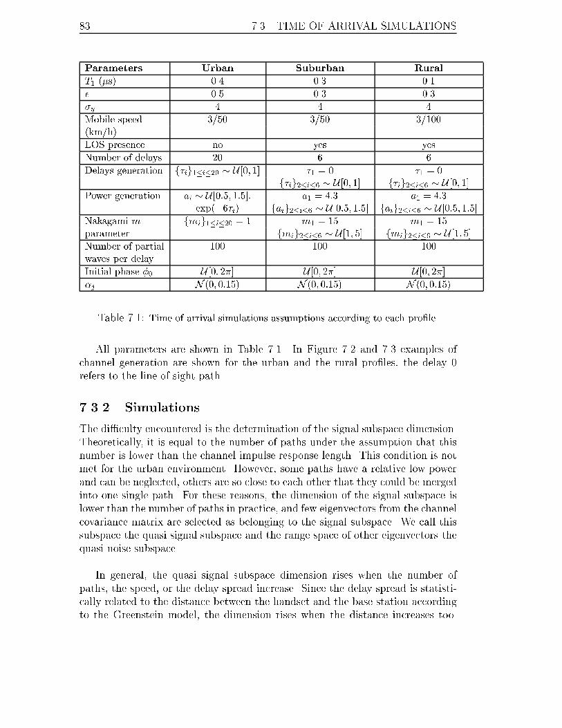
83 7.3. TIME OF ARRIVAL SIMULATIONS
Parameters Urban Suburban Rural
T1 (�s) 0.4 0.3 0.1
� 0.5 0.3 0.3
�y 4 4 4
Mobile speed 3/50 3/50 3/100
(km/h)
LOS presence no yes yes
Number of delays 20 6 6
Delays generation f�ig1�i�20 � U [0; 1] �1 = 0 �1 = 0
f�ig2�i�6 � U [0; 1] f�ig2�i�6 � U [0; 1]
Power generation ai � U [0:5; 1:5]: a1 = 4:3 a1 = 4:3
exp(�6�i) faig2�i�6 � U [0:5; 1:5] faig2�i�6 � U [0:5; 1:5]
Nakagami m fmig1�i�20 = 1 m1 = 15 m1 = 15
parameter fmig2�i�6 � U [1; 5] fmig2�i�6 � U [1; 5]
Number of partial 100 100 100
waves per delay
Initial phase �0 U [0; 2�] U [0; 2�] U [0; 2�]
�j N (0; 0:15) N (0; 0:15) N (0; 0:15)
Table 7.1: Time of arrival simulations assumptions according to each pro�le.
All parameters are shown in Table 7.1. In Figure 7.2 and 7.3 examples of
channel generation are shown for the urban and the rural pro�les, the delay 0
refers to the line of sight path.
7.3.2 Simulations
The di�culty encountered is the determination of the signal subspace dimension.
Theoretically, it is equal to the number of paths under the assumption that this
number is lower than the channel impulse response length. This condition is not
met for the urban environment. However, some paths have a relative low power
and can be neglected, others are so close to each other that they could be merged
into one single path. For these reasons, the dimension of the signal subspace is
lower than the number of paths in practice, and few eigenvectors from the channel
covariance matrix are selected as belonging to the signal subspace. We call this
subspace the quasi signal subspace and the range space of other eigenvectors the
quasi noise subspace.
In general, the quasi signal subspace dimension rises when the number of
paths, the speed, or the delay spread increase. Since the delay spread is statisti-
cally related to the distance between the handset and the base station according
to the Greenstein model, the dimension rises when the distance increases too.

CHAPTER 7. GLOBAL SIMULATIONS AND FINAL RESULTS 84
(a)0 0.1 0.2 0.3 0.4 0.5 0.6 0.7 0.8 0.9
0
0.1
0.2
0.3
0.4
0.5
0.6
0.7
0.8
0.9
µ s
Am
plitu
de
2 km/h
(b)0 0.1 0.2 0.3 0.4 0.5 0.6 0.7 0.8 0.9
0
0.1
0.2
0.3
0.4
0.5
0.6
0.7
0.8
µ s
Am
plitu
de
50 km/h
Figure 7.2: Urban pro�le example, 20 consecutive bursts are generated: (a) at 2 km/h,
(b) at 50 km/h. At high speed, the fading is less correlated in time. There is no line
of sight path and a bias in the ToA estimation is unavoidable.
The impact of the distance and the speed on the eigenvalues is depicted in Fig-
ures 7.4 and 7.5. The mean values of the strongest three eigenvalues are drawn.
It is shown that in most cases the �rst eigenvalue concentrates more than 90% of
the channel impulse response energy.
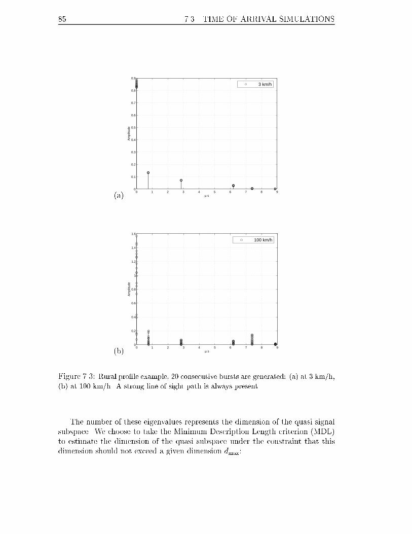
85 7.3. TIME OF ARRIVAL SIMULATIONS
(a)0 1 2 3 4 5 6 7 8 9
0
0.1
0.2
0.3
0.4
0.5
0.6
0.7
0.8
0.9
µ s
Am
plitu
de
3 km/h
(b)0 1 2 3 4 5 6 7 8 9
0
0.2
0.4
0.6
0.8
1
1.2
1.4
1.6
µ s
Am
plitu
de
100 km/h
Figure 7.3: Rural pro�le example, 20 consecutive bursts are generated: (a) at 3 km/h,
(b) at 100 km/h. A strong line of sight path is always present.
The number of these eigenvalues represents the dimension of the quasi signal
subspace. We choose to take the Minimum Description Length criterion (MDL)
to estimate the dimension of the quasi subspace under the constraint that this
dimension should not exceed a given dimension dmax:
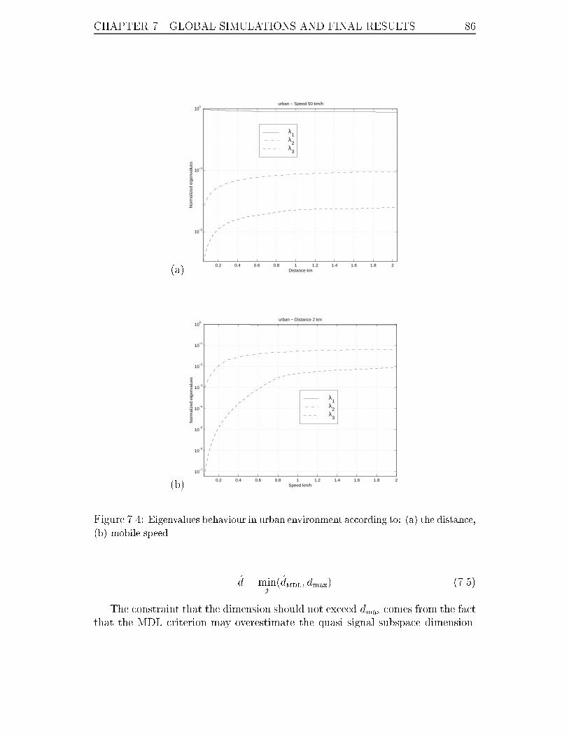
CHAPTER 7. GLOBAL SIMULATIONS AND FINAL RESULTS 86
(a)0.2 0.4 0.6 0.8 1 1.2 1.4 1.6 1.8 2
10−2
10−1
100
Distance km
Nor
mal
ized
eig
enva
lues
urban − Speed 50 km/h
λ1
λ2
λ3
(b)0.2 0.4 0.6 0.8 1 1.2 1.4 1.6 1.8 2
10−7
10−6
10−5
10−4
10−3
10−2
10−1
100
Speed km/h
Nor
mal
ized
eig
enva
lues
urban − Distance 2 km
λ1
λ2
λ3
Figure 7.4: Eigenvalues behaviour in urban environment according to: (a) the distance,
(b) mobile speed.
d = minj(dMDL; dmax) (7.5)
The constraint that the dimension should not exceed dmax comes from the fact
that the MDL criterion may overestimate the quasi signal subspace dimension.
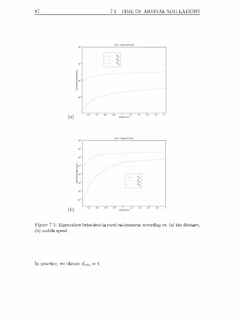
87 7.3. TIME OF ARRIVAL SIMULATIONS
(a)0.2 0.4 0.6 0.8 1 1.2 1.4 1.6 1.8 2
10−3
10−2
10−1
100
Distance km
Nor
mal
ized
eig
enva
lues
rural − Speed 100 km/h
λ1
λ2
λ3
(b)0.2 0.4 0.6 0.8 1 1.2 1.4 1.6 1.8 2
10−7
10−6
10−5
10−4
10−3
10−2
10−1
100
Speed km/h
Nor
mal
ized
eig
enva
lues
rural − Distance 10 km
λ1
λ2
λ3
Figure 7.5: Eigenvalues behaviour in rural environment according to: (a) the distance,
(b) mobile speed.
In practice, we choose dmax = 4.
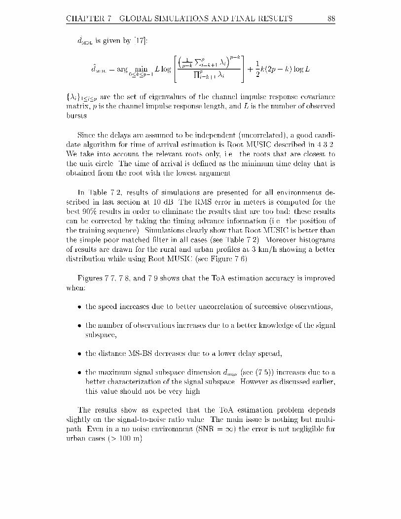
CHAPTER 7. GLOBAL SIMULATIONS AND FINAL RESULTS 88
dMDL is given by [17]:
dMDL = arg min0�k�p�1
L log
264�
1p�k
Pp
i=k+1 �i�p�k
Qp
i=k+1 �i
375+ 1
2k(2p� k) logL
f�ig1�i�p are the set of eigenvalues of the channel impulse response covariance
matrix, p is the channel impulse response length, and L is the number of observed
bursts.
Since the delays are assumed to be independent (uncorrelated), a good candi-
date algorithm for time of arrival estimation is Root MUSIC described in 4.3.2.
We take into account the relevant roots only, i.e. the roots that are closest to
the unit circle. The time of arrival is de�ned as the minimum time delay that is
obtained from the root with the lowest argument.
In Table 7.2, results of simulations are presented for all environments de-
scribed in last section at 10 dB. The RMS error in meters is computed for the
best 90% results in order to eliminate the results that are too bad: these results
can be corrected by taking the timing advance information (i.e. the position of
the training sequence). Simulations clearly show that Root MUSIC is better than
the simple poor matched �lter in all cases (see Table 7.2). Moreover histograms
of results are drawn for the rural and urban pro�les at 3 km/h showing a better
distribution while using Root MUSIC (see Figure 7.6).
Figures 7.7, 7.8, and 7.9 shows that the ToA estimation accuracy is improved
when:
� the speed increases due to better uncorrelation of successive observations,
� the number of observations increases due to a better knowledge of the signal
subspace,
� the distance MS-BS decreases due to a lower delay spread,
� the maximum signal subspace dimension dmax (see (7.5)) increases due to a
better characterization of the signal subspace. However as discussed earlier,
this value should not be very high.
The results show as expected that the ToA estimation problem depends
slightly on the signal-to-noise ratio value. The main issue is nothing but multi-
path. Even in a no noise environment (SNR = 1) the error is not negligible for
urban cases (> 100 m).

89 7.4. LOCATION SIMULATIONS
(a)−250 −200 −150 −100 −50 0 50 100 150
0
200
400
600
800
1000
1200
1400
1600
1800rural 3 km/h
Metres
Num
ber
of m
easu
rem
ents
Root MUSICMF
(b)−400 −200 0 200 400 600 800
0
200
400
600
800
1000
1200
1400urban 3 km/h
Metres
Num
ber
of m
easu
rem
ents
Root MUSICMF
Figure 7.6: ToA estimation error histogram at 3 km/h and 10 dB using 20 synch.
bursts for: (a) rural environment at 10 km, (b) urban environment at 1 km.
7.4 Location simulations
In this section, we combine the times of arrival estimation with the trilateration
procedure to get the �nal location.
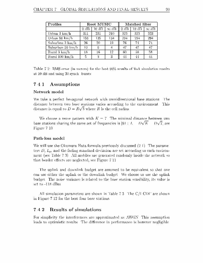
CHAPTER 7. GLOBAL SIMULATIONS AND FINAL RESULTS 90
Pro�les Root MUSIC Matched �lter
0 dB 10 dB 1 dB 0 dB 10 dB 1 dB
Urban 3 km/h 311 231 210 323 323 323
Urban 50 km/h 156 135 134 294 294 294
Suburban 3 km/h 26 20 19 76 74 74
Suburban 50 km/h 10 6 4 47 47 47
Rural 3 km/h 18 16 12 60 58 58
Rural 100 km/h 5 3 3 44 44 44
Table 7.2: RMS error (in meters) for the best 90% results of ToA simulation results
at 10 dB and using 20 synch. bursts.
7.4.1 Assumptions
Network model
We take a perfect hexagonal network with omnidirectional base stations. The
distance between two base stations varies according to the environment. This
distance is equal to D = Rp3 where R is the cell radius.
We choose a reuse pattern with K = 7. The minimal distance between two
base stations sharing the same set of frequencies is [81]: L = DpK = D
p7, see
Figure 7.10.
Path-loss model
We will use the Okumura-Hata formula previously discussed (2.1). The parame-
ters D, Lp, and the fading standard deviation are set according to each environ-
ment (see Table 7.3). All mobiles are generated randomly inside the network so
that border e�ects are neglected, see Figure 7.11.
The uplink and downlink budget are assumed to be equivalent so that one
can use either the uplink or the downlink budget. We choose to use the uplink
budget. The noise variance is related to the base station sensibility, its value is
set to -118 dBm.
All simulation parameters are shown in Table 7.3. The C/I CDF are shown
in Figure 7.12 for the best four base stations.
7.4.2 Results of simulations
For simplicity the interferences are approximated as AWGN. This assumption
leads to optimistic results. The di�erence in performance is however negligible.
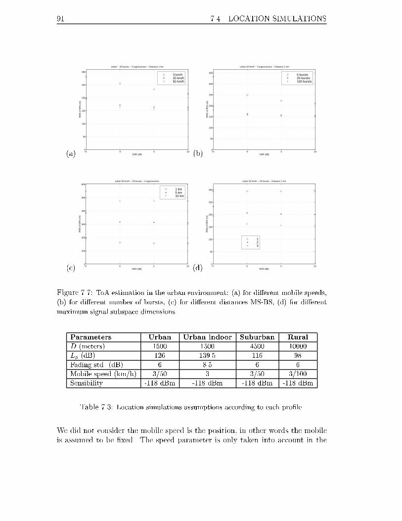
91 7.4. LOCATION SIMULATIONS
(a) −5 0 5 100
50
100
150
200
250
300
urban − 20 bursts − 3 eigenvectors − Distance 1 km
SNR (dB)
RM
S o
f 90%
(m
)
3 km/h20 km/h50 km/h
(b) −5 0 5 100
50
100
150
200
250
300
350
urban 50 km/h − 3 eigenvectors − Distance 1 km
SNR (dB)
RM
S o
f 90%
(m
)
5 bursts20 bursts100 bursts
(c) −5 0 5 100
100
200
300
400
500
600urban 50 km/h − 20 bursts − 3 eigenvectors
SNR (dB)
RM
S o
f 90%
(m
)
1 km5 km10 km
(d) −5 0 5 100
50
100
150
200
250
300
urban 50 km/h − 20 bursts − Distance 1 km
SNR (dB)
RM
S o
f 90%
(m
)
123
Figure 7.7: ToA estimation in the urban environment: (a) for di�erent mobile speeds,
(b) for di�erent number of bursts, (c) for di�erent distances MS-BS, (d) for di�erent
maximum signal subspace dimensions.
Parameters Urban Urban indoor Suburban Rural
D (meters) 1500 1500 4500 10000
Lp (dB) 126 139.5 116 98
Fading std. (dB) 6 8.5 6 6
Mobile speed (km/h) 3/50 3 3/50 3/100
Sensibility -118 dBm -118 dBm -118 dBm -118 dBm
Table 7.3: Location simulations assumptions according to each pro�le.
We did not consider the mobile speed is the position, in other words the mobile
is assumed to be �xed. The speed parameter is only taken into account in the
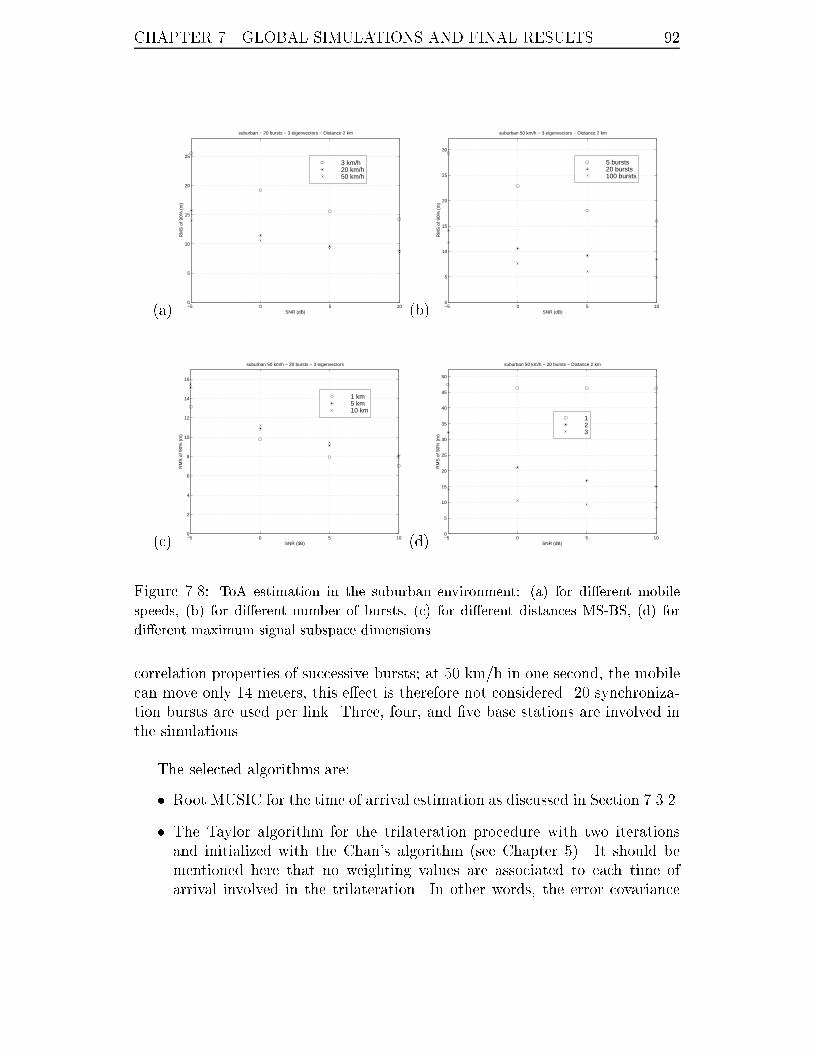
CHAPTER 7. GLOBAL SIMULATIONS AND FINAL RESULTS 92
(a) −5 0 5 100
5
10
15
20
25
suburban − 20 bursts − 3 eigenvectors − Distance 2 km
SNR (dB)
RM
S o
f 90%
(m
)
3 km/h20 km/h50 km/h
(b) −5 0 5 100
5
10
15
20
25
30
suburban 50 km/h − 3 eigenvectors − Distance 2 km
SNR (dB)
RM
S o
f 90%
(m
)
5 bursts20 bursts100 bursts
(c) −5 0 5 100
2
4
6
8
10
12
14
16
suburban 50 km/h − 20 bursts − 3 eigenvectors
SNR (dB)
RM
S o
f 90%
(m
)
1 km5 km10 km
(d) −5 0 5 100
5
10
15
20
25
30
35
40
45
50
suburban 50 km/h − 20 bursts − Distance 2 km
SNR (dB)
RM
S o
f 90%
(m
)
123
Figure 7.8: ToA estimation in the suburban environment: (a) for di�erent mobile
speeds, (b) for di�erent number of bursts, (c) for di�erent distances MS-BS, (d) for
di�erent maximum signal subspace dimensions.
correlation properties of successive bursts; at 50 km/h in one second, the mobile
can move only 14 meters, this e�ect is therefore not considered. 20 synchroniza-
tion bursts are used per link. Three, four, and �ve base stations are involved in
the simulations.
The selected algorithms are:
� Root MUSIC for the time of arrival estimation as discussed in Section 7.3.2.
� The Taylor algorithm for the trilateration procedure with two iterations
and initialized with the Chan's algorithm (see Chapter 5). It should be
mentioned here that no weighting values are associated to each time of
arrival involved in the trilateration. In other words, the error covariance
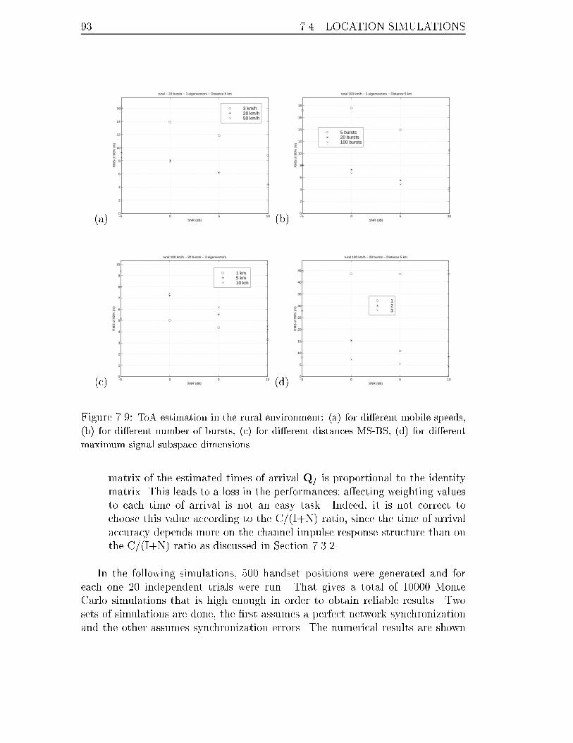
93 7.4. LOCATION SIMULATIONS
(a) −5 0 5 100
2
4
6
8
10
12
14
16
rural − 20 bursts − 3 eigenvectors − Distance 5 km
SNR (dB)
RM
S o
f 90%
(m
)
3 km/h20 km/h50 km/h
(b) −5 0 5 100
2
4
6
8
10
12
14
16
18
rural 100 km/h − 3 eigenvectors − Distance 5 km
SNR (dB)
RM
S o
f 90%
(m
)
5 bursts20 bursts100 bursts
(c) −5 0 5 100
1
2
3
4
5
6
7
8
9
10
rural 100 km/h − 20 bursts − 3 eigenvectors
SNR (dB)
RM
S o
f 90%
(m
)
1 km5 km10 km
(d) −5 0 5 100
5
10
15
20
25
30
35
40
45
rural 100 km/h − 20 bursts − Distance 5 km
SNR (dB)
RM
S o
f 90%
(m
)
123
Figure 7.9: ToA estimation in the rural environment: (a) for di�erent mobile speeds,
(b) for di�erent number of bursts, (c) for di�erent distances MS-BS, (d) for di�erent
maximum signal subspace dimensions.
matrix of the estimated times of arrival Qf is proportional to the identity
matrix. This leads to a loss in the performances; a�ecting weighting values
to each time of arrival is not an easy task. Indeed, it is not correct to
choose this value according to the C/(I+N) ratio, since the time of arrival
accuracy depends more on the channel impulse response structure than on
the C/(I+N) ratio as discussed in Section 7.3.2.
In the following simulations, 500 handset positions were generated and for
each one 20 independent trials were run. That gives a total of 10000 Monte
Carlo simulations that is high enough in order to obtain reliable results. Two
sets of simulations are done, the �rst assumes a perfect network synchronization
and the other assumes synchronization errors. The numerical results are shown
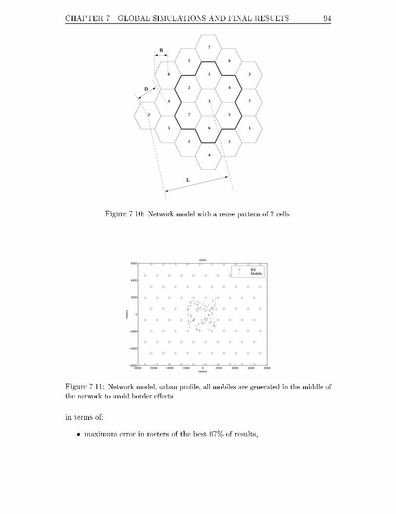
CHAPTER 7. GLOBAL SIMULATIONS AND FINAL RESULTS 94
1
2
3
4
5
6
7
4
3
5
1
4
2
1
7
2
6
7
5
6
L
D
R
Figure 7.10: Network model with a reuse pattern of 7 cells.
−8000 −6000 −4000 −2000 0 2000 4000 6000 8000−6000
−4000
−2000
0
2000
4000
6000
meters
met
ers
urban
BSMobile
Figure 7.11: Network model, urban pro�le, all mobiles are generated in the middle of
the network to avoid border e�ects.
in terms of:
� maximum error in meters of the best 67% of results,

95 7.4. LOCATION SIMULATIONS
(a) −15 −10 −5 0 5 10 15 20 25 3010
−3
10−2
10−1
100
urban
C/I (dB)
CD
F (
%)
(b) −15 −10 −5 0 5 10 15 20 25 3010
−3
10−2
10−1
100
urban indoor
C/I (dB)
CD
F (
%)
(c) −15 −10 −5 0 5 10 15 20 25 3010
−3
10−2
10−1
100
rural
C/I (dB)
CD
F (
%)
(d) −15 −10 −5 0 5 10 15 20 25 3010
−3
10−2
10−1
100
suburban
C/I (dB)
CD
F (
%)
Figure 7.12: C/I CDF for the BCCH channel for the serving cell and the nearest three
base stations: urban pro�les are interference limited while rural and suburban pro�les
are noise limited.
� percentage of results with an error lower than 125 meters,
� root mean square error of the best 90 % of results.
Perfect knowledge of the RTDs
Perfect synchronization is assumed in these simulations. The results are depicted
in Table 7.4. In general, an improvement is observed when the number of base
stations involved in the procedure rises. There is an anomaly in the urban case;
the results using �ve base stations (shown in bold) are slightly worse than with
four. The reason for that is related to the wrong weighting of the times of arrival
before data fusion. The improvement is very signi�cant with four base stations
compared to three. Indeed, with three base stations there is no extra information

CHAPTER 7. GLOBAL SIMULATIONS AND FINAL RESULTS 96
since three is the minimum number of base stations required.
Pro�les 67 % in meters Percentage < 125 m RMS of 90%
3 BS 4 BS 5 BS 3 BS 4 BS 5 BS 3 BS 4 BS 5 BS
Urban out. 3 km/h 104 93 93 72 76 78 115 84 80
Urban out. 50 km/h 95 83 84 74 79 82 104 76 72
Urban in. 3 km/h 108 94 97 71 75 77 119 86 82
Suburban 3 km/h 17 12 12 91 98 98 20 12 12
Suburban 50 km/h 12 8 8 93 100 100 12 7 7
Rural 3 km/h 6 5 5 90 100 100 10 4 4
Rural 100 km/h 4 3 3 91 100 100 5 3 3
Table 7.4: Location simulations results with three, four, and �ve base stations. Net-
work perfectly synchronized.
Synchronization errors
The relative o�set of each base station is assumed to be corrupted with a Gaus-
sian noise with zero mean and a standard variation of 100 ns which corresponds
to approximately 30 meters. Results are shown in Table 7.5 and shown in term
of CDF curves for all speci�ed environments in Figures 7.13, 7.14, 7.16, and 7.15.
Pro�les 67 % in meters Percentage < 125 m RMS of 90%
3 BS 4 BS 5 BS 3 BS 4 BS 5 BS 3 BS 4 BS 5 BS
Urban out. 3 km/h 116 99 99 69 75 76 124 90 85
Urban out. 50 km/h 106 91 89 72 78 80 111 81 77
Urban in. 3 km/h 120 103 100 69 74 76 130 92 86
Suburban 3 km/h 49 38 34 91 98 98 42 31 28
Suburban 50 km/h 46 35 31 93 100 100 39 28 25
Rural 3 km/h 47 34 30 90 100 100 42 28 25
Rural 100 km/h 45 33 29 90 100 100 39 27 24
Table 7.5: Location simulations results with three, four, and �ve base stations. Syn-
chronization errors are included.
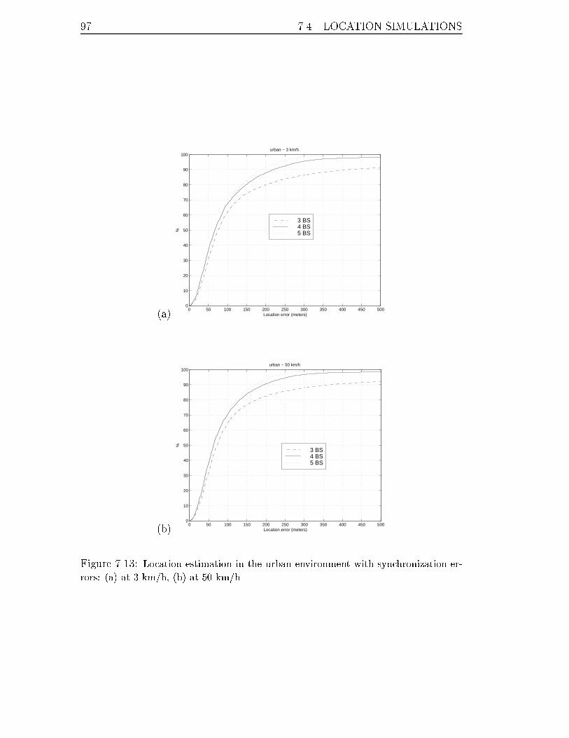
97 7.4. LOCATION SIMULATIONS
(a)0 50 100 150 200 250 300 350 400 450 500
0
10
20
30
40
50
60
70
80
90
100
Location error (meters)
%
urban − 3 km/h
3 BS4 BS5 BS
(b)0 50 100 150 200 250 300 350 400 450 500
0
10
20
30
40
50
60
70
80
90
100
Location error (meters)
%
urban − 50 km/h
3 BS4 BS5 BS
Figure 7.13: Location estimation in the urban environment with synchronization er-
rors: (a) at 3 km/h, (b) at 50 km/h.
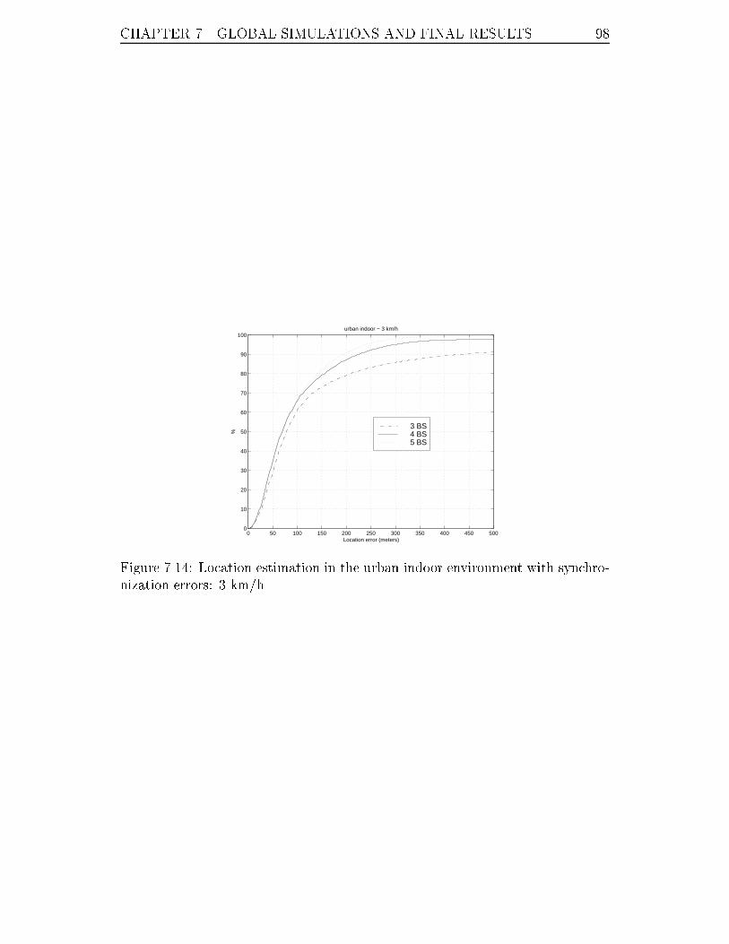
CHAPTER 7. GLOBAL SIMULATIONS AND FINAL RESULTS 98
0 50 100 150 200 250 300 350 400 450 5000
10
20
30
40
50
60
70
80
90
100
Location error (meters)
%
urban indoor − 3 km/h
3 BS4 BS5 BS
Figure 7.14: Location estimation in the urban indoor environment with synchro-
nization errors: 3 km/h.
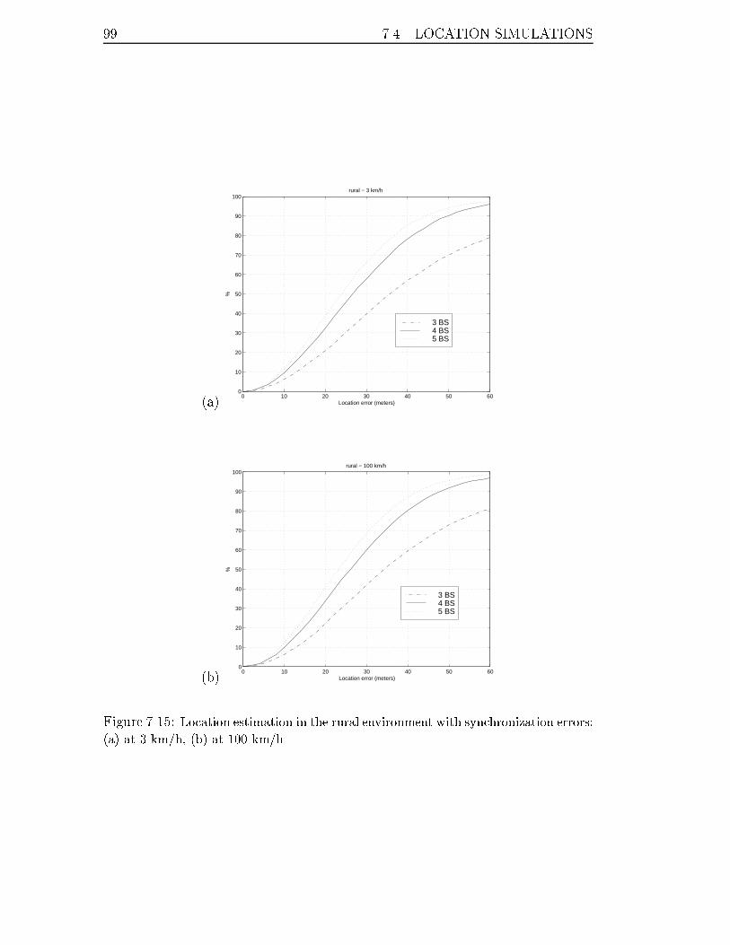
99 7.4. LOCATION SIMULATIONS
(a)0 10 20 30 40 50 60
0
10
20
30
40
50
60
70
80
90
100
Location error (meters)
%
rural − 3 km/h
3 BS4 BS5 BS
(b)0 10 20 30 40 50 60
0
10
20
30
40
50
60
70
80
90
100
Location error (meters)
%
rural − 100 km/h
3 BS4 BS5 BS
Figure 7.15: Location estimation in the rural environment with synchronization errors:
(a) at 3 km/h, (b) at 100 km/h.
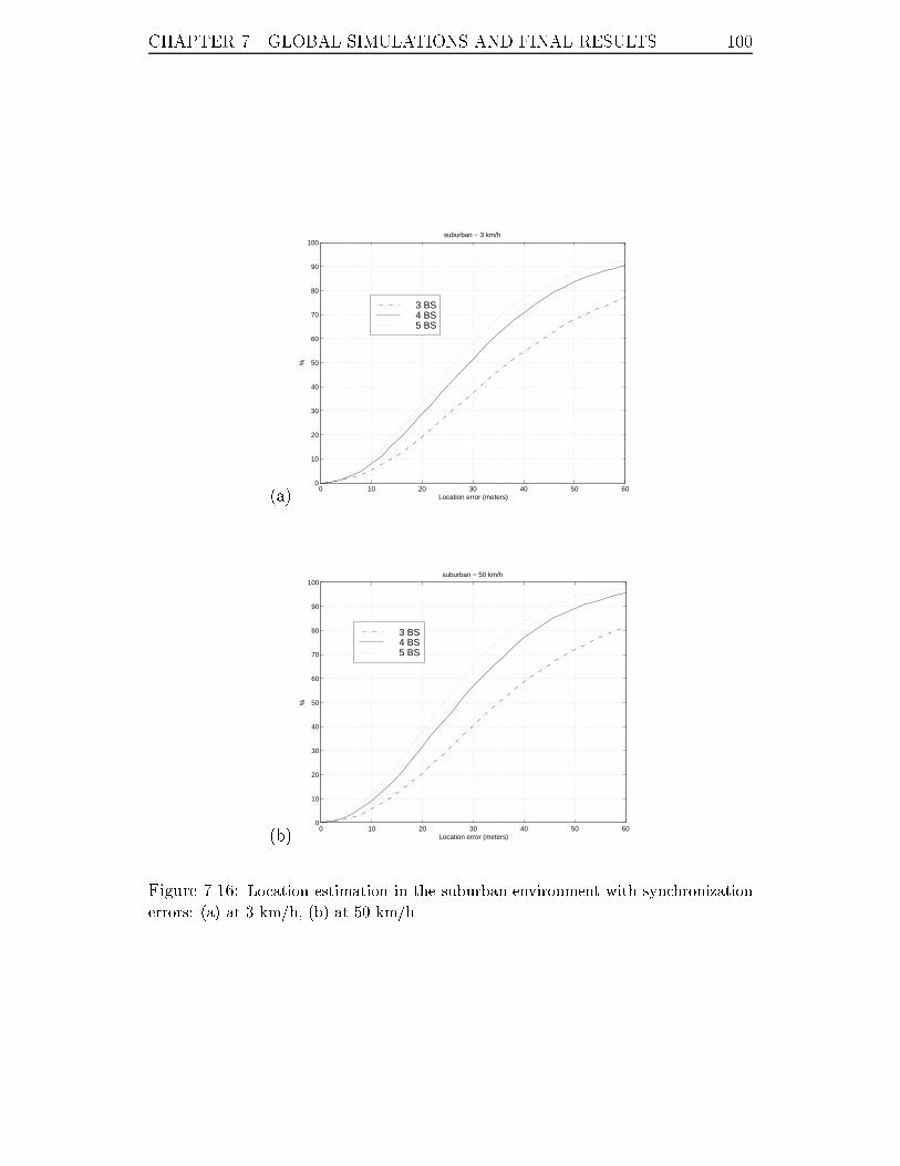
CHAPTER 7. GLOBAL SIMULATIONS AND FINAL RESULTS 100
(a)0 10 20 30 40 50 60
0
10
20
30
40
50
60
70
80
90
100
Location error (meters)
%
suburban − 3 km/h
3 BS4 BS5 BS
(b)0 10 20 30 40 50 60
0
10
20
30
40
50
60
70
80
90
100
Location error (meters)
%
suburban − 50 km/h
3 BS4 BS5 BS
Figure 7.16: Location estimation in the suburban environment with synchronization
errors: (a) at 3 km/h, (b) at 50 km/h.
Chapter 8
Conclusion and further research
In this dissertation, we have presented a global system for locating a mobile
handset in a GSM network. This system makes use of the own capability of the
network.
We have shown that the best technology for this purpose is based on time
of arrival estimation either at the handset, at the base station, or even both for
more accuracy. The main source of problems in time of arrival estimation is mul-
tipath. Based on the maximum likelihood estimator, subspace �tting algorithms
are applied to estimate the time delays of the dominant paths. The time of arrival
is simply the path that has the lowest time delay. An extension is presented to
the case of an unknown modulation pulse shape. Two approaches are considered:
the �rst one is iterative, it begins with a �rst initialization of the pulse shape
and converges iteratively to the true one. The second approach is a variant of
the well-known ESPRIT algorithm, it is non iterative and has a lower complexity.
Hyperbolic trilateration is then analyzed and appears to be a non linear max-
imization problem. The scoring approach seems to o�er optimal performances at
high signal-to-noise ratios and good results at lowest ratios whenever an appro-
priate initialization is available.
Network synchronization is depicted. A distinction is made between pseudo
and absolute synchronization. An algorithm is presented for each approach.
The last chapter presented the global system taking the channel model estab-
lished in the T1P1.5 committee.
Some aspects have not been treated in this manuscript and might be impor-
tant to complete the study:
101
CHAPTER 8. CONCLUSION AND FURTHER RESEARCH 102
Di�use paths
In this work, we assume that each path arrived at one discrete time delay (spec-
ular path). An interesting extension is the case of di�use paths. In this scenario
the partial waves of each path arrive around a mean value.
The correct model for the channel impulse response must be modi�ed as
follows:
hj(t) =dX
i=1
KiXk=1
sijka(t� �i � ~�ik) 1 � j � L (8.1)
This topic has been studied recently, two main approaches exist:
� Taylor expansion [82, 83].
� The spreading in time is assumed to follow a certain distribution (mainly
uniform or Gaussian) centered on the delay and a joint estimation of the
distribution mean and variance is performed [84{86].
CRB for the unknown pulse shape case
When we estimate the delays assuming an unknown modulation pulse, the com-
parison of the performances has been done using the standard CRB. Computing
the CRB for an unknown modulation pulse shape is di�cult to achieve but might
be interesting.
Optimal weighting
No weighting factor or covariance matrix were applied to the times of arrival while
performing the trilateration. It is of course possible to use empirical weighting
based on the signal-to-noise ratio or the channel impulse response delay spread.
Finding such values remains an open question.
CDMA systems - UMTS
Localization is a requirement is future standards such as the Universal Mobile
Telecommunications System (UMTS). Unlike GSM, UMTS is a wideband system
based on Direct-Sequence Code Division Multiple Access (DS CDMA).
Chapter 9
R�esum�e d�etaill�e en fran�cais
9.1 Introduction
Depuis que le concept cellulaire fut introduit dans les ann�ees soixante, les commu-
nications sans �l ont connu un d�eveloppement sans pr�ec�edent. Il existe actuelle-
ment di��erents standards. Le syst�eme europ�een GSM est sans doute le standard
le plus r�epandu de nos jours. Ce syst�eme est bas�e sur l'acc�es multiple des utilisa-
teurs �a la fois en temps et en fr�equence. Plusieurs utilisateurs peuvent communi-
quer depuis la meme zone sur la meme fr�equence en se partageant �equitablement
le temps d'�emission.
En juin 1996, le comit�e f�ed�eral am�ericain de communication (FCC) a de-
mand�e aux op�erateurs am�ericains de localiser les appels d'urgence �emanant de
leurs abonn�es avec une pr�ecision de 125 m�etres dans 67 pour cent des cas d�es
octobre 2001.
La localisation est souvent associ�ee au GPS. Ce syst�eme o�re une couverture
compl�ete du globe terrestre mais demeure peu �able en zone urbaine. L'objet
de cette th�ese est de montrer qu'il est possible d'o�rir un service de localisation
�able en utilisant les infra-structures d�ej�a existantes des r�eseaux GSM. L'�etude
porte sur la localisation par estimation du temps d'arriv�ee d'au moins trois canaux
correspondant �a di��erentes stations de base. L'estimation de la position s'e�ectue
alors moyennant des donn�ees de synchronisation des di��erentes stations de base
impliqu�ees.
103
CHAPTER 9. R�ESUM�E D�ETAILL�E EN FRANC�AIS 104
9.2 Communications sans �l
9.2.1 Mod�ele de propagation radio
� Mod�ele d'att�enuation : au fur et �a mesure que les ondes radio se propagent,
elles perdent de l'intensit�e. Ainsi dans l'espace libre, la d�ecroissance de
l'�energie est inversement proportionnelle au carr�e de la distance parcourue.
Il existe de nombreux mod�eles empiriques de propagation. Ceux-ci reposent
en g�en�eral sur des mesures de terrain. Le mod�ele d'Okumura-Hata est le
mod�ele le plus couramment utilis�e.
� Evanouissements lent et rapide : outre l'att�enuation due �a la distance
parcourue, le signal radio est sujet �a d'autres uctuations ; uctuations
lentes dues aux masquages provoqu�es par des obstacles physiques et uc-
tuations rapides dues �a la r�e exion du signal sur une surface. En e�et,
le signal r�e �echi provient de la contribution de plusieurs r�e exions locales
d'amplitudes et de phases di��erentes. Ces r�e exions peuvent ainsi s'ajouter
ou s'annuler provoquant ainsi des uctuations rapides de l'enveloppe du sig-
nal re�cu.
� Trajet multiple et �etalement temporel : le signal radio subit des r�e exions
multiples. Chaque r�e exion se caract�erise par une �energie moyenne et
une phase. Le signal re�cu se compose ainsi d'une multitude de copies.
L'enveloppe r de chaque copie est mod�elis�ee par une loi de distribution de
Rayleigh :
p(r) =r
�2e�
r2
2�2 (9.1)
�2 = E [jxj2] d�esigne l'�energie moyenne de l'�echo. En revanche, le trajet
direct, s'il existe, n'est pas de moyenne nulle, son enveloppe suit la loi de
distribution de Rice :
p(r) =r
�2e�
r2+m
2
2�2 I0
�rm
�2
�(9.2)
o�u m2 = jE[x]j2 et �2 = E [jx� E[x]j2].
L'�etalement temporel est un param�etre important qui caract�erise l'environnement,
il est donn�e par :
� =qm2 �m2
1 (9.3)
o�u mp =
Piai�
p
iPiai
est le moment d'ordre p du signal. ai et �i sont respective-
ment l'�energie moyenne et le retard du i-i�eme trajet. Yuanking [3] a montr�e
par des mesures de terrain que cette quantit�e suit une loi de distribution
al�eatoire qui d�epend de la distance parcourue :
� � T1d�y (9.4)
105 9.2. COMMUNICATIONS SANS FIL
T1 et � sont deux constantes qui d�ependent de l'environnement. d est la
distance parcourue et y est une variable log-normale.
� Interf�erences : dans un syst�eme de communication cellulaire, la ressource ra-
dio est rare. Elle est ainsi partag�ee et r�eutilis�ee. Ceci introduit in�evitablement
des interf�erences qu'il faut minimiser lors de la planni�cation cellulaire.
Nous ferons l'approximation que les interf�erences sont gaussiennes (approx-
imation AWGN). Cette hypoth�ese est justi��ee si le nombre d'interf�ereurs est
su�samment �elev�e. Cette hypoth�ese simpli�e �enorm�ement les simulations
car les interf�ereurs ne seront pas g�en�er�es individuellement mais l'ensemble
sera g�en�er�e par une seule variable gaussienne.
� Ecart Doppler : lorsque le mobile bouge, le signal radio est sujet �a l'e�et
Doppler qui le translate en fr�equence. Cet �ecart est d'autant plus important
que la vitesse est grande. A 900 Mhz, l'�ecart maximal est �a peu pr�es �egal
�a un Hertz par km/h.
Il existe di��erents moyens de protection comme le codage de canal, l'entrelacement,
la transmission discontinue de parole (DTX), le controle de puissance, le saut de
fr�equence, la diversit�e spatiale et l'utilisation de s�equences d'apprentissage.
9.2.2 Aper�cu de la norme GSM
Le syst�eme GSM est bas�e sur la combinaison de deux technologies ; l'acc�es mul-
tiple par r�epartition �a la fois en temps et en fr�equence. Un groupe de fr�equences
porteuses est allou�e �a chaque cellule. Plusieurs mobiles peuvent communiquer
sur la meme fr�equence en utilisant chacun une portion de temps. Le domaine
temporel est ainsi d�ecoup�e en cycles de communication ou trames. Chaque trame
se compose de huit portions de temps d�edi�ees chacune �a un utilisateur. Une por-
tion de temps est de longueur 577 �s. En g�en�eral, le temps de coh�erence (ou
m�emoire) du canal radio est plus long. Cette hypoth�ese justi�e le fait que la
r�eponse impulsionnelle du canal est constante pendant la dur�ee d'une portion de
temps.
Le canal physique duplex
Les fronts de communication montant (mobile vers station de base) et descen-
dant (station de base vers mobile) sont s�epar�es en temps et en fr�equence. Il y
a trois portions de temps de d�ecalage et un �ecart fr�equentiel constant entre ces
deux fronts. Un canal physique GSM repr�esente l'association de deux portions
de temps sur les deux fronts. On parle donc de canal physique duplex.
Chaque portion de temps accueille une s�equence de bits d'information ap-
pel�ee burst. Celle-ci a une dur�ee inf�erieure �a la dur�ee de la portion de temps
CHAPTER 9. R�ESUM�E D�ETAILL�E EN FRANC�AIS 106
pour �eviter tout chevauchement d'un burst sur le suivant. Le burst repr�esente
l'information v�ehicul�ee et il existe sous di��erents formats. Il contient toujours une
s�equence d'apprentissage de bits pr�ed�e�nie et une s�equence de bits d'information.
La s�equence d'apprentissage sert �a aider le r�ecepteur �a identi�er le canal radio
pour faciliter la r�ecup�eration des donn�ees. Les bursts normaux ont une s�equence
d'apprentissage de 26 bits, les bursts d'acc�es 48 bits et les burst de synchronisa-
tion 64 bits.
Les canaux logiques
Les trames de huit portions de temps sont organis�ees en multi-trames de 26 ou
51 trames selon la nature de l'information qu'elles v�ehiculent : tra�c ou signal-
isation. On parle ainsi de canaux logiques dont on distingue les canaux d�edi�es
qui fonctionnent en mode duplex (tra�c) et les canaux de signalisation qui ne
fonctionnent que sur un seul front montant ou descendant.
La modulation GMSK
La modulation utilis�ee en GSM est une modulation de phase �a enveloppe con-
stante appel�ee GMSK. Cependant, il est toujours possible d'approximer une mod-
ulation de phase �a codage di��erentiel par une modulation lin�eaire [6]. Dans ce
cas, le signal re�cu s'exprime de mani�ere simple :
s(t) �Xk
dka(t� kT ) (9.5)
o�u dk d�esigne la s�equence de bits �emise et a(t) l'impulsion principale de la mod-
ulation GMSK. Cette impulsion s'�etale sur quatre temps bits.
9.2.3 Egalisation
L'�egalisation consiste �a d�emoduler le signal pour en d�eduire une estimation des
bits d'information �emis. A la r�eception, le signal r�esulte de la convolution du
signal d'�emission par le �ltre d'�emission et le �ltre repr�esent�e par la r�eponse
impulsionnelle du canal, le tout �etant noy�e dans du bruit blanc suppos�e gaussien
si bien qu'�a l'arriv�ee le signal s'�ecrit sous la forme suivante :
y(t) =p�1Xk=0
dkh(t� kT ) + b(t) (9.6)
La fonction h(t) est commun�ement appel�ee r�eponse impulsionnelle du canal
meme si elle int�egre tous les �ltres mis en jeu (modulation, �emission, canal
et r�eception). Il est important de pouvoir estimer la r�eponse impulsionnelle
pour pouvoir �egaliser. Cette estimation s'e�ectue par le biais de la s�equence
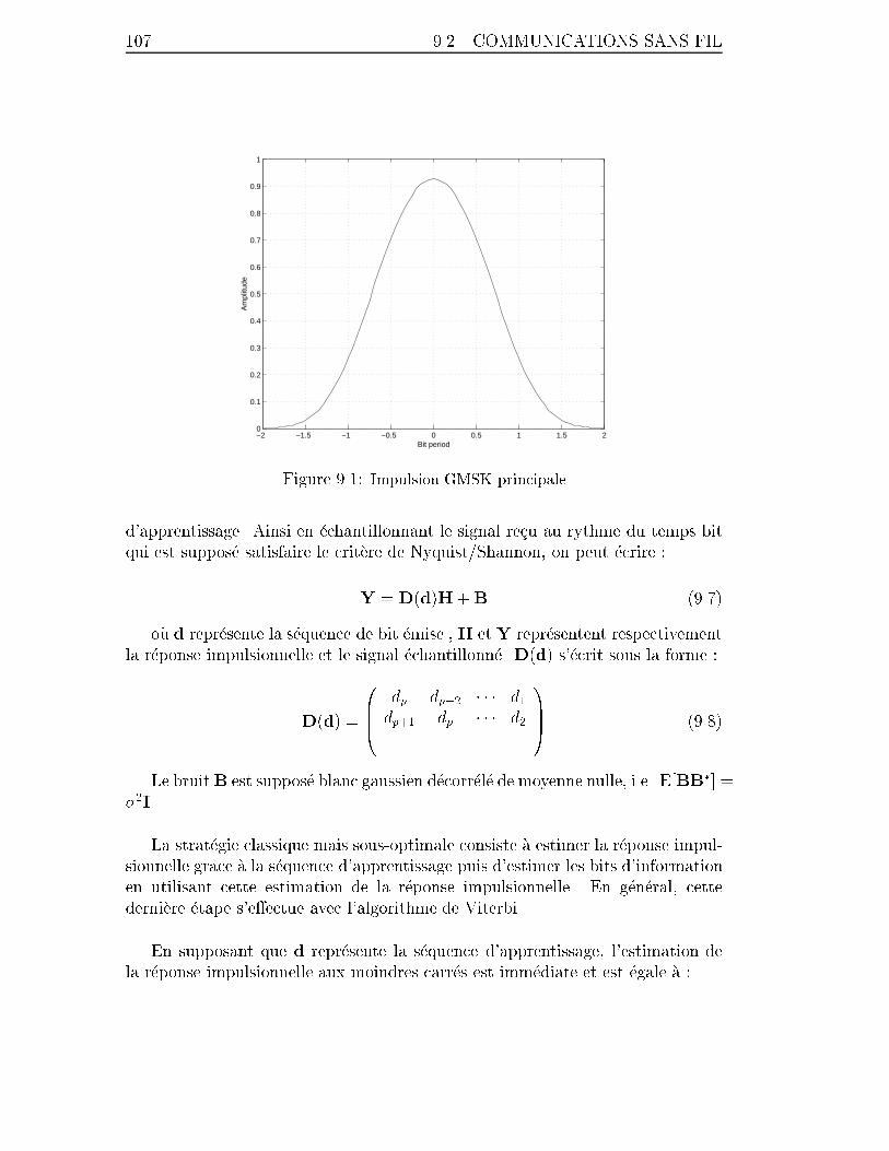
107 9.2. COMMUNICATIONS SANS FIL
−2 −1.5 −1 −0.5 0 0.5 1 1.5 20
0.1
0.2
0.3
0.4
0.5
0.6
0.7
0.8
0.9
1
Bit period
Am
plitu
de
Figure 9.1: Impulsion GMSK principale
d'apprentissage. Ainsi en �echantillonnant le signal re�cu au rythme du temps bit
qui est suppos�e satisfaire le crit�ere de Nyquist/Shannon, on peut �ecrire :
Y = D(d)H+B (9.7)
o�u d repr�esente la s�equence de bit �emise , H et Y repr�esentent respectivement
la r�eponse impulsionnelle et le signal �echantillonn�e. D(d) s'�ecrit sous la forme :
D(d) =
0BB@
dp dp�2 � � � d1dp+1 dp � � � d2...
......
1CCA (9.8)
Le bruitB est suppos�e blanc gaussien d�ecorr�el�e de moyenne nulle, i.e. E[BB�] =
�2I.
La strat�egie classique mais sous-optimale consiste �a estimer la r�eponse impul-
sionnelle grace �a la s�equence d'apprentissage puis d'estimer les bits d'information
en utilisant cette estimation de la r�eponse impulsionnelle. En g�en�eral, cette
derni�ere �etape s'e�ectue avec l'algorithme de Viterbi.
En supposant que d repr�esente la s�equence d'apprentissage, l'estimation de
la r�eponse impulsionnelle aux moindres carr�es est imm�ediate et est �egale �a :

CHAPTER 9. R�ESUM�E D�ETAILL�E EN FRANC�AIS 108
H = Dy(d)Y (9.9)
Dy = [D�D]�1D� d�esigne la pseudo-inverse de D.
9.3 Technologies pour la localisation
Dans cette partie, di��erentes technologies sont pr�esent�ees pour localiser un mo-
bile. Nous nous e�orcerons d'expliquer pourquoi l'approche bas�ee sur l'estimation
du temps d'arriv�ee semble etre la plus plausible.
Estimation de la distance
C'est sans doute la m�ethode la plus intuitive et la plus directe. Il s'agit d'estimer
la distance parcourue par le signal re�cu en mesurant son intensit�e �a la r�eception.
La puissance �a l'�emission est connue �a travers le param�etre de controle de puis-
sance. En utilisant une formule simple de propagation il est possible d'avoir une
estimation de la distance. En r�ep�etant le meme principe sur deux stations de
base, trouver la position du mobile devient possible en calculant l'intersection de
deux cercles.
Reconnaissance �a base d'apprentissage
Cette m�ethode ressemble au probl�eme de la reconnaissance de caract�ere o�u, �a
partir de mesures diverses, on essaie de trouver la zone de localisation la plus
probable dans laquelle le mobile est susceptible de se trouver. Cette d�ecision
s'e�ectue moyennant une base d'apprentissage compos�ee de mesures recueillies
sur le terrain.
Angle d'arriv�ee
C'est une technique connue qui a suscit�e de nombreuses publications ces derni�eres
d�ecennies. Il s'agit d'estimer l'angle d'arriv�ee d'un signal sur un r�eseau de
plusieurs capteurs espac�es d'une longueur d'onde.
Temps d'arriv�ee
L'estimation du temps d'arriv�ee est une ancienne technique utilis�ee dans de nom-
breuses applications. Dans le contexte GSM, cette estimation s'e�ectue grace �a
la s�equence d'apprentissage. Deux sc�enarii sont possibles selon que les mesures
s'e�ectuent sur le front montant ou descendant.

109 9.4. ESTIMATION DU TEMPS D'ARRIV�EE
9.4 Estimation du temps d'arriv�ee
9.4.1 Notations et hypoth�eses
Nous partons du principe que la r�eponse impulsionnelle du canal se compose de
d r�e exions discr�etes. Chaque r�e exion est caract�eris�ee par un retard et une
amplitude complexe :
hj(t) =dX
i=1
sija(t� �i) 1 � j � L (9.10)
L'indice j porte sur la j-i�eme r�ealisation. En e�et la r�eponse impulsionnelle
du canal, suppos�ee constante pendant la dur�ee d'un burst varie d'un burst �a
l'autre. Pour obtenir la meilleure estimation possible, il faut accumuler un max-
imum d'observations. a(t) est l'impulsion GMSK principale. sij est l'amplitude
complexe associ�ee au i-i�eme retard lors de l'�emission du j-i�eme burst. Seuls les
retards �i sont suppos�es constants pendant la dur�ee d'observation des L bursts.
Le trajet direct n'est pas toujours pr�esent. Le but est d'estimer le retard du
premier trajet d'�energie su�samment �elev�ee pour qu'il puisse etre d�etect�e. La
strat�egie choisie pour cela est d'estimer la totalit�e des retards puis de choisir le
premier comme �etant le temps d'arriv�ee.
9.4.2 Approche temporelle
Cette approche consiste �a traiter le signal re�cu dans le domaine temporel. En
�echantillonnant au rythme du temps bit, celui-ci s'�ecrit sous la forme suivante :
Yj = D(d)A(�)Sj +Nj 1 � j � L (9.11)
Il existe deux versions du maximum de vraisemblance selon la connaissance
que l'on a sur le vecteur des amplitudes complexes Sj. En e�et, si ce vecteur
ne suit pas une loi de distribution al�eatoire ou que sa loi est tout simplement
inconnue, alors il faut estimer les amplitudes instantan�ees conjointement avec les
retards, ceci donne le maximum de vraisemblance d�eterministe dont l'expression
r�eduite qu'il faut maximiser par rapport �a � s'�ecrit :
VDML(�) = Trh�?D(d)A(�)Ky
i(9.12)
En revanche si l'on suppose que ces amplitudes sont gaussiennes de moyennes
nulles alors il faudra estimer leur matrice de covarianceKs conjointement avec les
retards. Ceci donne le maximum de vraisemblance stochastique dont l'expression
r�eduite qu'il faut maximiser par rapport �a � est :
VSML(�) = ln���D(d)A(�)Ks(�) [D(d)A(�)]
�+ �2(�)I
��� (9.13)
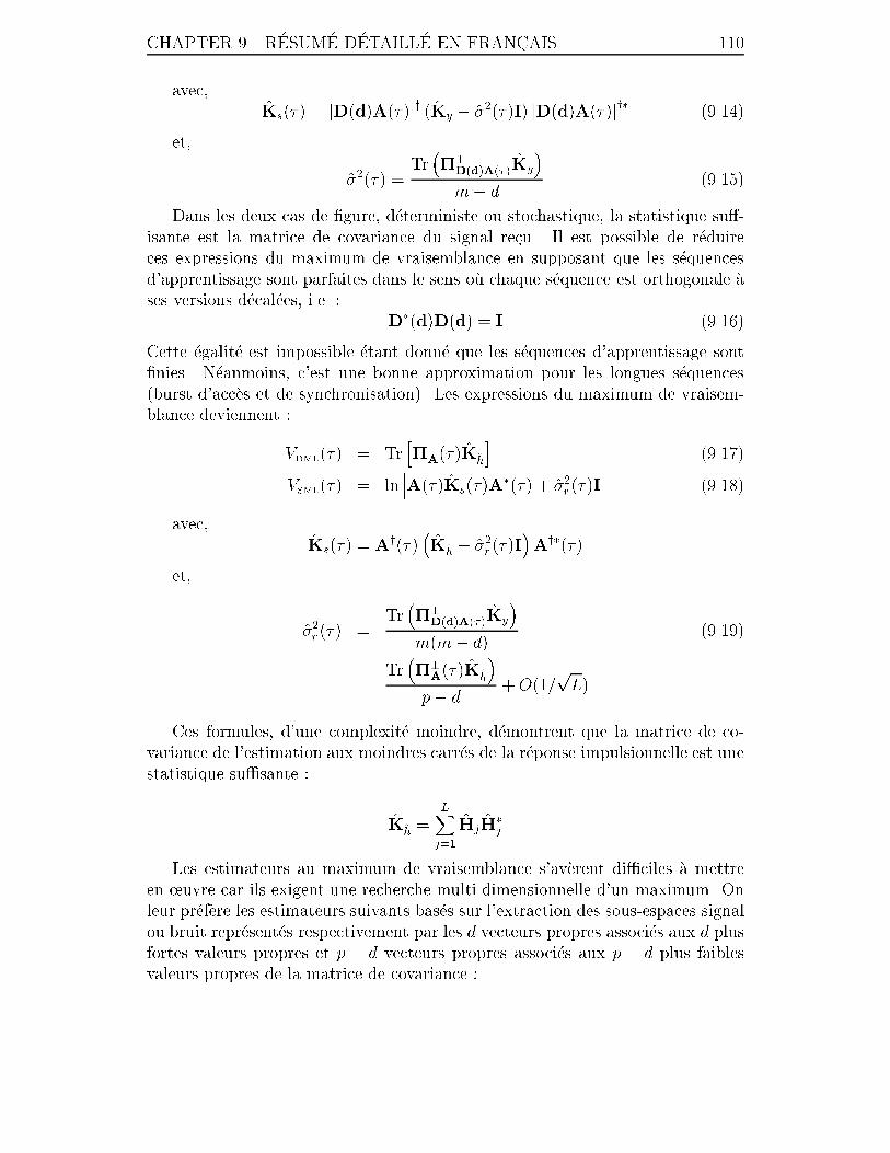
CHAPTER 9. R�ESUM�E D�ETAILL�E EN FRANC�AIS 110
avec,
Ks(�) = [D(d)A(�)]y(Ky � �2(�)I) [D(d)A(�)]
y�(9.14)
et,
�2(�) =Tr��?D(d)A(�)Ky
�m� d
(9.15)
Dans les deux cas de �gure, d�eterministe ou stochastique, la statistique su�-
isante est la matrice de covariance du signal re�cu. Il est possible de r�eduire
ces expressions du maximum de vraisemblance en supposant que les s�equences
d'apprentissage sont parfaites dans le sens o�u chaque s�equence est orthogonale �a
ses versions d�ecal�ees, i.e. :
D�(d)D(d) = I (9.16)
Cette �egalit�e est impossible �etant donn�e que les s�equences d'apprentissage sont
�nies. N�eanmoins, c'est une bonne approximation pour les longues s�equences
(burst d'acc�es et de synchronisation). Les expressions du maximum de vraisem-
blance deviennent :
VDML(�) = Trh�?A(�)K
h
i(9.17)
VSML(�) = ln���A(�)Ks(�)A
�(�) + �2r(�)I
��� (9.18)
avec,
Ks(�) = Ay(�)�K
h� �2
r(�)I
�Ay�(�)
et,
�2r(�) =
Tr��?D(d)A(�)Ky
�m(m� d)
(9.19)
=Tr��?A(�)K
h
�p� d
+O(1=pL)
Ces formules, d'une complexit�e moindre, d�emontrent que la matrice de co-
variance de l'estimation aux moindres carr�es de la r�eponse impulsionnelle est une
statistique su�sante :
Kh=
LXj=1
HjH�j
Les estimateurs au maximum de vraisemblance s'av�erent di�ciles �a mettre
en �uvre car ils exigent une recherche multi dimensionnelle d'un maximum. On
leur pr�ef�ere les estimateurs suivants bas�es sur l'extraction des sous-espaces signal
ou bruit repr�esent�es respectivement par les d vecteurs propres associ�es aux d plus
fortes valeurs propres et p � d vecteurs propres associ�es aux p � d plus faibles
valeurs propres de la matrice de covariance :
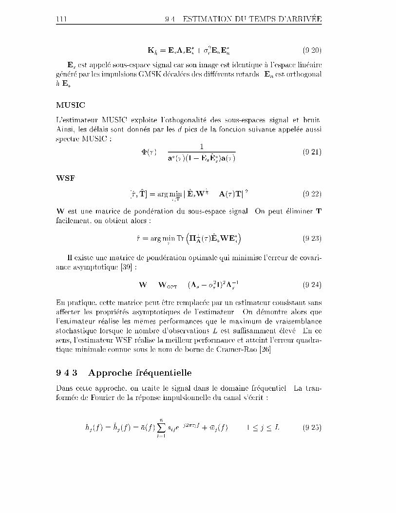
111 9.4. ESTIMATION DU TEMPS D'ARRIV�EE
Kh= Es�sE
�s+ �2
rEnE
�n
(9.20)
Es est appel�e sous-espace signal car son image est identique �a l'espace lin�eaire
g�en�er�e par les impulsions GMSK d�ecal�ees des di��erents retards. En est orthogonal
�a Es.
MUSIC
L'estimateur MUSIC exploite l'othogonalit�e des sous-espaces signal et bruit.
Ainsi, les d�elais sont donn�es par les d pics de la fonction suivante appel�ee aussi
spectre MUSIC :
�(�) =1
a�(�)(I� EsE�s)a(�)
(9.21)
WSF
[� ; T] = argmin�;T
kEsW1
2 �A(�)Tk2 (9.22)
W est une matrice de pond�eration du sous-espace signal. On peut �eliminer T
facilement, on obtient alors :
� = argmin�
Tr��?A(�)EsWE�
s
�(9.23)
Il existe une matrice de pond�eration optimale qui minimise l'erreur de covari-
ance asymptotique [39] :
W =WOPT = (�s � �2rI)2��1
s(9.24)
En pratique, cette matrice peut etre remplac�ee par un estimateur consistant sans
a�ecter les propri�et�es asymptotiques de l'estimateur. On d�emontre alors que
l'estimateur r�ealise les memes performances que le maximum de vraisemblance
stochastique lorsque le nombre d'observations L est su�samment �elev�e. En ce
sens, l'estimateur WSF r�ealise la meilleur performance et atteint l'erreur quadra-
tique minimale connue sous le nom de borne de Cramer-Rao [26].
9.4.3 Approche fr�equentielle
Dans cette approche, on traite le signal dans le domaine fr�equentiel. La tran-
form�ee de Fourier de la r�eponse impulsionnelle du canal s'�ecrit :
�hj(f) = ~hj(f) = �a(f)
nXi=1
sije�j2��if + �wj(f) 1 � j � L (9.25)
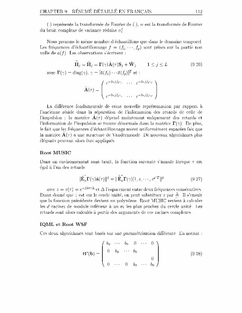
CHAPTER 9. R�ESUM�E D�ETAILL�E EN FRANC�AIS 112
�(:) repr�esente la transform�ee de Fourier de (:), �w est la transform�ee de Fourier
du bruit complexe de variance r�eduite �2r.
Nous prenons le meme nombre d'�echantillons que dans le domaine temporel.
Les fr�equences d'�echantillonnage f = (f1; � � � ; fp) sont prises sur la partie non
nulle de �a(f). Les observations s'�ecrivent :
�Hj = ~Hj = �( ) ~A(�)Sj + �Wj 1 � j � L (9.26)
avec �( ) = diag( ), = [�a(f1) � � � �a(fp)]T et :
~A(�) =
0BB@e�2�jf1�1 � � � e�2�jf1�d
......
e�2�jfp�1 � � � e�2�jfp�d
1CCA
La di��erence fondamentale de cette nouvelle repr�esentation par rapport �a
l'ancienne r�eside dans la s�eparation de l'information des retards de celle de
l'impulsion ; la matrice ~A(�) d�epend maintenant uniquement des retards et
l'information de l'impulsion se trouve d�esormais dans la matrice �( ). De plus,
le fait que les fr�equences d'�echantillonnage soient uniform�ement espac�ees fait que
la matrice ~A(�) a une structure de Vandermonde. De nouvaux algorithmes plus
�el�egants peuvent alors etre appliqu�es.
Root MUSIC
Dans un environnement sans bruit, la fonction suivante s'annule lorsque � est
�egal �a l'un des retards.
k ~E�
n�( )~a(�)k2 = k ~E
�
n�( )[1; z; � � � ; zp]Tk2 (9.27)
avec z = z(�) = e�j2��� et � l'espacement entre deux fr�equences cons�ecutives.
Etant donn�e que z est sur le cercle unit�e, on peut substituer z par 1z�. Il s'ensuit
que la fonction pr�ec�edente devient un polynome. Root MUSIC revient �a calculer
les d racines de module inf�erieur �a un et les plus proches du cercle unit�e. Les
retards sont alors calcul�es �a partir des arguments de ces racines complexes.
IQML et Root WSF
Ces deux algorithmes sont bas�es sur une param�etrisation di��erente. En notant :
B�(b) =
0BBBBB@
bd � � � b0 0 � � � 0
0 bd � � � b0. . .
......
. . .. . .
. . . 0
0 � � � 0 bd � � � b0
1CCCCCA (9.28)
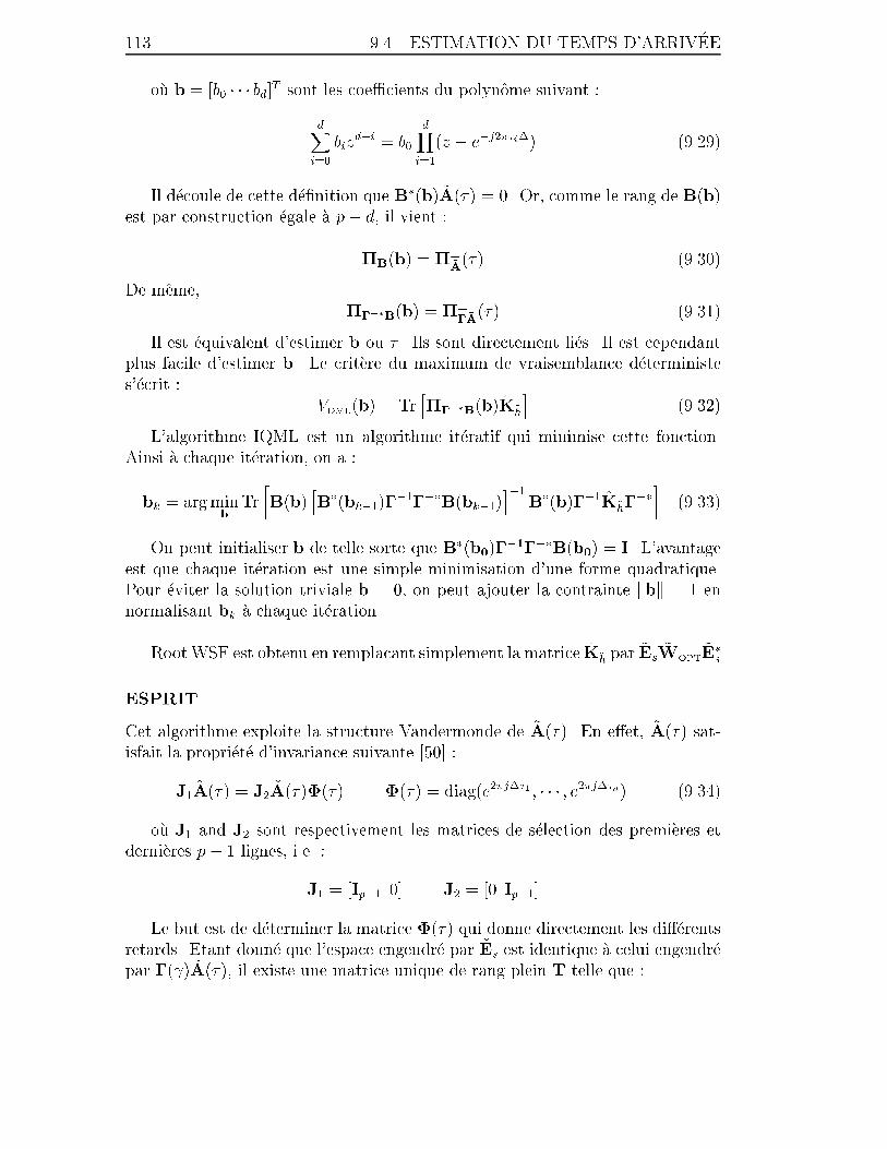
113 9.4. ESTIMATION DU TEMPS D'ARRIV�EE
o�u b = [b0 � � � bd]T sont les coe�cients du polynome suivant :
dXi=0
bizd�i = b0
dYi=1
(z � e�j2��i�) (9.29)
Il d�ecoule de cette d�e�nition que B�(b) ~A(�) = 0. Or, comme le rang de B(b)
est par construction �egale �a p� d, il vient :
�B(b) = �?~A(�) (9.30)
De meme,
����B(b) = �?�~A
(�) (9.31)
Il est �equivalent d'estimer b ou � . Ils sont directement li�es. Il est cependant
plus facile d'estimer b. Le crit�ere du maximum de vraisemblance d�eterministe
s'�ecrit :
VDML(b) = Trh����B(b)K~h
i(9.32)
L'algorithme IQML est un algorithme it�eratif qui minimise cette fonction.
Ainsi �a chaque it�eration, on a :
bk = argminb
Tr
�B(b)
hB�(bk�1)�
�1���B(bk�1)i�1
B�(b)��1K~h����
(9.33)
On peut initialiser b de telle sorte que B�(b0)��1���B(b0) = I. L'avantage
est que chaque it�eration est une simple minimisation d'une forme quadratique.
Pour �eviter la solution triviale b = 0, on peut ajouter la contrainte kbk = 1 en
normalisant bk �a chaque it�eration.
RootWSF est obtenu en remplacant simplement la matrice K~h par~Es
~WOPT~E�s.
ESPRIT
Cet algorithme exploite la structure Vandermonde de ~A(�). En e�et, ~A(�) sat-
isfait la propri�et�e d'invariance suivante [50] :
J1 ~A(�) = J2 ~A(�)�(�) �(�) = diag(e2�j��1 ; � � � ; e2�j��d) (9.34)
o�u J1 and J2 sont respectivement les matrices de s�election des premi�eres et
derni�eres p� 1 lignes, i.e. :
J1 = [Ip�1 0] J2 = [0 Ip�1]
Le but est de d�eterminer la matrice �(�) qui donne directement les di��erents
retards. Etant donn�e que l'espace engendr�e par ~Es est identique �a celui engendr�e
par �( ) ~A(�), il existe une matrice unique de rang plein T telle que :
CHAPTER 9. R�ESUM�E D�ETAILL�E EN FRANC�AIS 114
J1 ~Es = J1�( ) ~A(�)T J2 ~Es = J2�( ) ~A(�)T
En notant �1, la matrice � apr�es �elimination de sa derni�ere ligne et derni�ere
colonne, et �2, la matrice � apr�es �elimination de sa premi�ere ligne et premi�ere
colonne, on peut �ecrire :
J1 ~Es = �1J1 ~A(�)T J2Es = �2J2 ~A(�)T
La propri�et�e d'invariance donne alors :
J1 ~Es = �1J2 ~A(�)�(�)T J2 ~Es = �2J2 ~A(�)T
soit :
�2��11 J1 ~Es = J2 ~Es(t) (9.35)
Avec (t) = T�1�(�)T. Les valeurs propres de (t) sont identiques �a celles
de � et donnent donc les retards. Pour estimer (t), on peut utiliser une simple
estimation aux moindres carr�es :
(�) =
�J2 ~Es
�y�2�
�11 J1 ~Es
9.4.4 Extension au cas d'une modulation inconnue
Les algorithmes pr�esent�es dans les sections pr�ec�edentes supposent une connais-
sance parfaite de la forme de l'impulsion de modulation. Ces algorithmes sont
cependant sensibles �a une d�eformation de cette impulsion. Une erreur, meme
minime, sur la forme de cette impulsion peut engendrer un biais important dans
les r�esultats d'estimation. Il est di�cile en pratique d'avoir une connaissance
parfaite car cette impulsion est modi��ee par les �ltres d'�emission et de r�eception,
ceux-ci pouvant etre di��erents d'un constructeur �a l'autre.
Nous proposons ici une extension dans le cas o�u l'impulsion est totalement
inconnue. En e�et, il est possible d'estimer conjointement l'impulsion et les
retards �a une r�ef�erence temporelle absolue pr�es, i.e. on est capable d'estimer
les di��erences entre les di��erents retards sans pouvoir toutefois en d�eduire leur
valeur. Ceci ne pose pas de probl�eme pour la localisation �etant donn�e que
seules les di��erences de temps d'arriv�ee nous interesse. Il est n�eanmoins pos-
sible d'estimer le temps absolu en utilisant une simple information a priori sur
l'impulsion. On utilisera l'information que l'impulsion de modulation est r�eelle
et sym�etrique pour se d�ebarasser de cette ambigu��t�e.

115 9.4. ESTIMATION DU TEMPS D'ARRIV�EE
Approche it�erative
La m�ethode la plus directe est de reprendre l'id�ee que le sous-espace signal est
engendr�e par ~Es.
[ � ]T= argmax
;�
dXi=1
k ~E�
s�( )~a(�i)k2 (9.36)
qui est �equivalent �a :
[ � ]T= argmax
;� �
dXi=1
D�i~Es~E�
sDi (9.37)
o�u Di = diag [~a(�i)]. est donc le vecteur propre associ�e �a la valeur propre
maximale de la matriceP
d
i=1D�i~Es
~E�
sDi �a un facteur multiplicatif pr�es. Ce fac-
teur multiplicatif peut etre d�etermin�e grace aux hypoth�eses faites sur l'impulsion.
L'id�ee est donc de partir d'une estimation initiale des retards et d'en d�eduire ainsi
la forme de l'impulsion repr�esent�ee par le vecteur . Une fois cette estimation
disponible, on estime �a nouveau les retards en utilisant un algorithme quelconque
et ainsi de suite jusqu'�a ce qu'une convergence soit atteinte.
Approche non it�erative
En reprenant la meme id�ee que l'estimateur ESPRIT et en notantD(�) = diag(�)
la matrice diagonale �2��11 , et (�) = T�1�(�)T, l'estimateur conjoint s'�ecrit
de la mani�ere suivante :
[� (�)]T = argmin�
kD(�)J1Es � J2Es(�)k2 (9.38)
La solution de ce probl�eme est donn�ee par :
(�) =�J2Es
�yD(�)J1Es
En incorporant cette equation dans (9.38), on obtient [60] :
� = argmin�
TrhD(�)J1EsE
�sJT1D
�(�)�?J2Es
i= argmin
���h�?J2Es
� J1(EsE�s)TJT1
i�
� est �egal au vecteur propre associ�e �a la valeur propre minimale de la matrice
�?J2Es
� J1(EsE�s)TJT1 �a un facteur multiplicatif pr�es. Ce facteur multiplicatif
peut etre d�etermin�e grace aux hypoth�eses faites sur l'impulsion.
Di��erence de temps d'arriv�ee
Dans les deux algorithmes d�ecrits pr�ec�edemment, un facteur multiplicatif in-
connu persiste si aucune hypoth�ese sur l'impulsion n'est disponible. En fait dans
les deux cas, seule la phase de ce facteur a une in uence sur l'estimation des
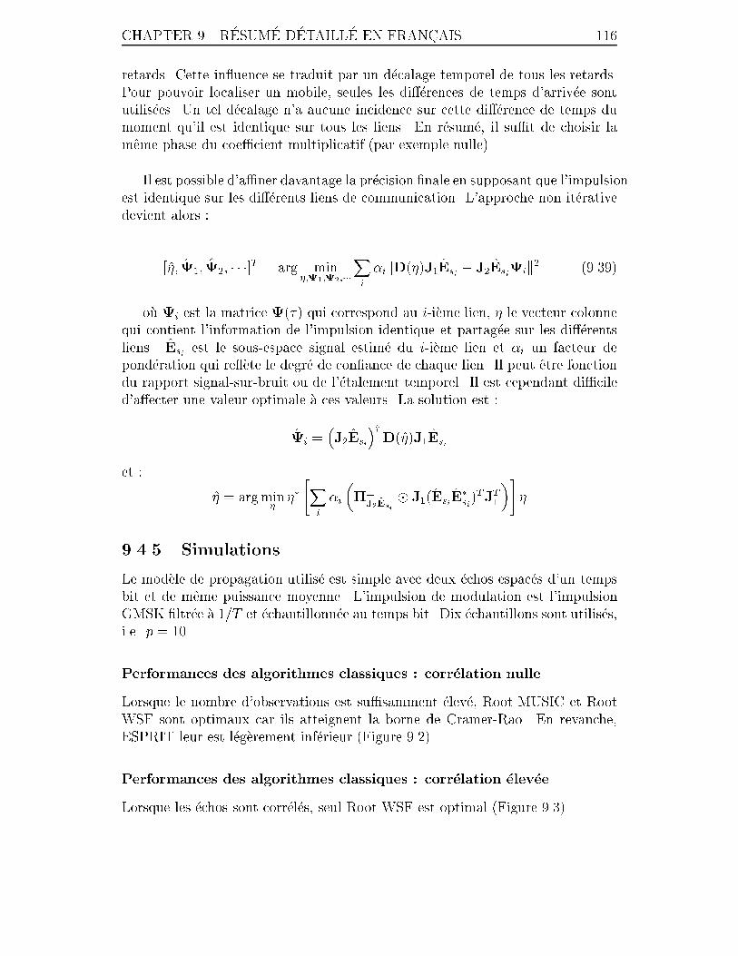
CHAPTER 9. R�ESUM�E D�ETAILL�E EN FRANC�AIS 116
retards. Cette in uence se traduit par un d�ecalage temporel de tous les retards.
Pour pouvoir localiser un mobile, seules les di��erences de temps d'arriv�ee sont
utilis�ees. Un tel d�ecalage n'a aucune incidence sur cette di��erence de temps du
moment qu'il est identique sur tous les liens. En r�esum�e, il su�t de choisir la
meme phase du coe�cient multiplicatif (par exemple nulle).
Il est possible d'a�ner davantage la pr�ecision �nale en supposant que l'impulsion
est identique sur les di��erents liens de communication. L'approche non it�erative
devient alors :
[�; 1; 2; � � �]T = arg min�;1;2;���
Xi
�ikD(�)J1Esi� J2Esi
ik2 (9.39)
o�u i est la matrice (�) qui correspond au i-i�eme lien, � le vecteur colonne
qui contient l'information de l'impulsion identique et partag�ee sur les di��erents
liens. Esiest le sous-espace signal estim�e du i-i�eme lien et �i un facteur de
pond�eration qui re �ete le degr�e de con�ance de chaque lien. Il peut etre fonction
du rapport signal-sur-bruit ou de l'�etalement temporel. Il est cependant di�cile
d'a�ecter une valeur optimale �a ces valeurs. La solution est :
i =�J2Esi
�yD(�)J1Esi
et :
� = argmin���"X
i
�i
��?J2Esi
� J1(EsiE�si)TJT1
�#�
9.4.5 Simulations
Le mod�ele de propagation utilis�e est simple avec deux �echos espac�es d'un temps
bit et de meme puissance moyenne. L'impulsion de modulation est l'impulsion
GMSK �ltr�ee �a 1=T et �echantillonn�ee au temps bit. Dix �echantillons sont utilis�es,
i.e. p = 10.
Performances des algorithmes classiques : corr�elation nulle
Lorsque le nombre d'observations est su�samment �elev�e, Root MUSIC et Root
WSF sont optimaux car ils atteignent la borne de Cramer-Rao. En revanche,
ESPRIT leur est l�eg�erement inf�erieur (Figure 9.2).
Performances des algorithmes classiques : corr�elation �elev�ee
Lorsque les �echos sont corr�el�es, seul Root WSF est optimal (Figure 9.3).
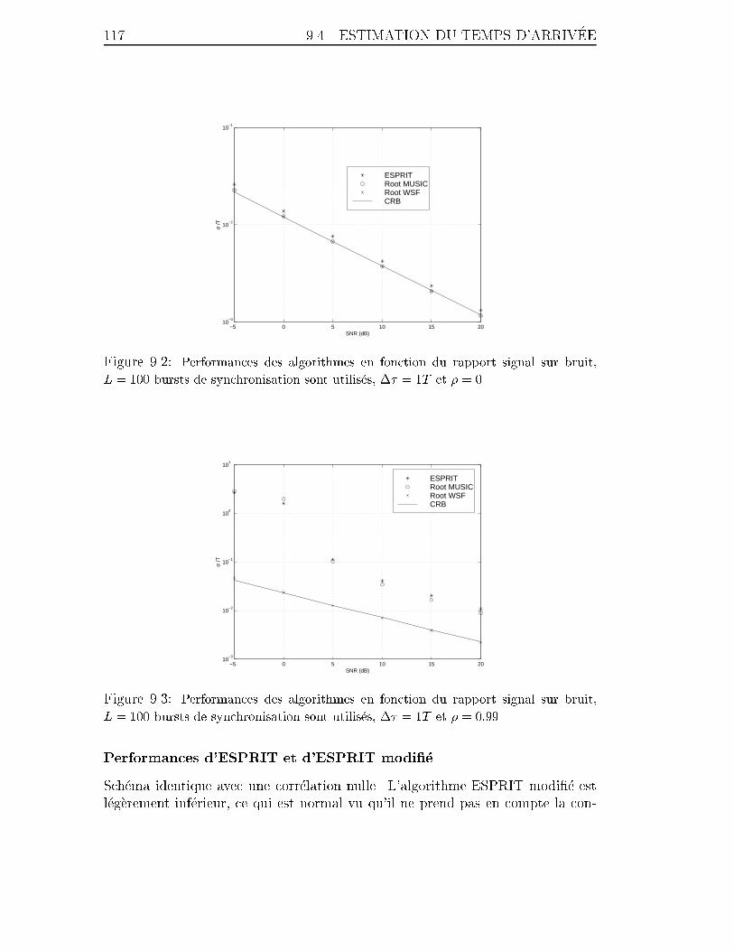
117 9.4. ESTIMATION DU TEMPS D'ARRIV�EE
−5 0 5 10 15 2010
−3
10−2
10−1
SNR (dB)
σ /T
ESPRITRoot MUSICRoot WSFCRB
Figure 9.2: Performances des algorithmes en fonction du rapport signal sur bruit,
L = 100 bursts de synchronisation sont utilis�es, �� = 1T et � = 0.
−5 0 5 10 15 2010
−3
10−2
10−1
100
101
SNR (dB)
σ /T
ESPRITRoot MUSICRoot WSFCRB
Figure 9.3: Performances des algorithmes en fonction du rapport signal sur bruit,
L = 100 bursts de synchronisation sont utilis�es, �� = 1T et � = 0:99.
Performances d'ESPRIT et d'ESPRIT modi��e
Sch�ema identique avec une corr�elation nulle. L'algorithme ESPRIT modi��e est
l�eg�erement inf�erieur, ce qui est normal vu qu'il ne prend pas en compte la con-
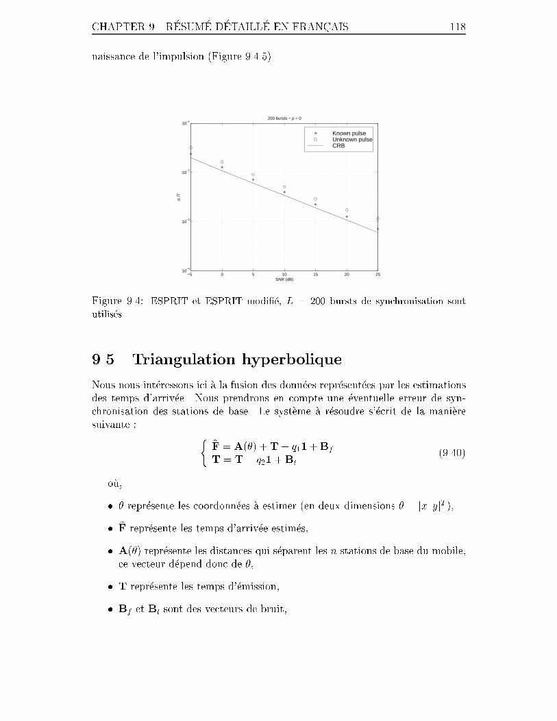
CHAPTER 9. R�ESUM�E D�ETAILL�E EN FRANC�AIS 118
naissance de l'impulsion (Figure 9.4.5).
−5 0 5 10 15 20 2510
−4
10−3
10−2
10−1
200 bursts − ρ = 0
SNR (dB)
σ /T
Known pulseUnknown pulseCRB
Figure 9.4: ESPRIT et ESPRIT modi��e, L = 200 bursts de synchronisation sont
utilis�es.
9.5 Triangulation hyperbolique
Nous nous int�eressons ici �a la fusion des donn�ees repr�esent�ees par les estimations
des temps d'arriv�ee. Nous prendrons en compte une �eventuelle erreur de syn-
chronisation des stations de base. Le syst�eme �a r�esoudre s'�ecrit de la mani�ere
suivante : (~F = A(�) +T� q11+Bf
�T = T� q21+Bt
(9.40)
o�u,
� � repr�esente les coordonn�ees �a estimer (en deux dimensions � = [x y]T ),
� ~F repr�esente les temps d'arriv�ee estim�es,
� A(�) repr�esente les distances qui s�eparent les n stations de base du mobile,
ce vecteur d�epend donc de �,
� T repr�esente les temps d'�emission,
� Bf et Bt sont des vecteurs de bruit,
119 9.5. TRIANGULATION HYPERBOLIQUE
� q1 et q2 sont deux temps de r�ef�erence inconnus,
� 1 = [1 � � �1]T .
On supposera que les deux vecteurs de bruit Bf and Bt sont gaussiens de
moyenne nulle :
� E[BfBT
f] = Qf
� E[BtBT
t] = Qt
� E[BfBT
t] = 0
Il est possible d'exprimer ce syst�eme sous forme compacte par :
F = A(�)� tr1+B (9.41)
o�u F = ~F� �T. Cette �equation aboutit �a une triangulation hyperbolique. Le
nombre de stations de base n doit etre strictement sup�erieur �a deux si on localise
en deux dimensions. Il y a trois variables �a estimer ; les coordonn�ees et le temps
de r�ef�erence tr. Bien entendu, lorsque n augmente, l'erreur d'estimation se trouve
r�eduite.
L'estimateur du maximum de vraisemblance s'�ecrit :
[� tr] = argmax�;tr
[F�A(�)� tr1]TQ�1 [F�A(�)� tr1] (9.42)
En �eliminant tr, on obtient une expression plus compacte :
� = argmax�
[F�A(�)]T ~Q [F�A(�)] (9.43)
avec,
~Q = Q�1 � Q�111TQ�1
1TQ�11
D�eveloppement en s�erie de Taylor
C'est un algorithme it�eratif qui cherche �a minimiser directement le crit�ere du
maximum de vraisemblance. Chaque it�eration s'�ecrit de la mani�ere suivante :
�n = �n�1 +
24 @A(�n�1)
@�
!T
~Q@A(�n�1)
@�
35�1
@A(�n�1)
@�
!T
~Q [F�A(�n�1)]
(9.44)
La convergence de cet algorithme d�epend en grande partie de son initialisation.
CHAPTER 9. R�ESUM�E D�ETAILL�E EN FRANC�AIS 120
M�ethode des moindres carr�es
Cette m�ethode est bas�ee sur une reformulation des �equations. Ainsi en �ecrivant
les n� 1 �equations suivantes :
(ri � r1)(ri + r1) = r2i� r21 2 � i � n
o�u ri d�esigne la distance entre le mobile et la i-i�eme station de base. On peut
obtenir le syst�eme compact suivant :
[HA(�)]� [(H�H)A(�)] = �2HJ� +HK (9.45)
o�u H d�esigne la matrice (n� 1)� n suivante :
H =
2666664
�1 1 0 � � � 0
�1 0 1. . .
......
.... . .
. . . 0
�1 0 � � � 0 1
3777775 (9.46)
et,
J =1
c2
2664x1 y1...
...
xn yn
3775 K =
1
c2
2664x21 + y21
...
x2n+ y2
n
3775 (9.47)
Notons que les �el�ements de HA(�) sont les di��erences de temps d'arriv�ee
(DToA) entre la i-i�eme station de base et la station de base courante �a laquelle
le mobile est connect�e. Soit, apr�es quelques manipulations alg�ebriques :
[HA(�)]� [HA(�)]�HK = �2HJ� � 2r1
cHA(�) (9.48)
Sans perte de g�en�eralit�es, nous pouvons consid�erer que la station de base
courante est �a l'origine, soit de mani�ere �equivalente r1 = j�j. L'�equation prend
alors la forme suivante :
1
2HK� 1
2[HF]� [HF] = HJ� +
j�jcHF +B1 (9.49)
A fort rapport signal sur bruit, on peut n�egliger les termes d'ordre deux du
bruit, et B1 demeure gaussien de moyenne nulle :
B1 � �RHB
o�u R = 1cdiag(r2; � � � ; rn). Sa covariance s'�ecrit :
Q1 = RHTQHR (9.50)
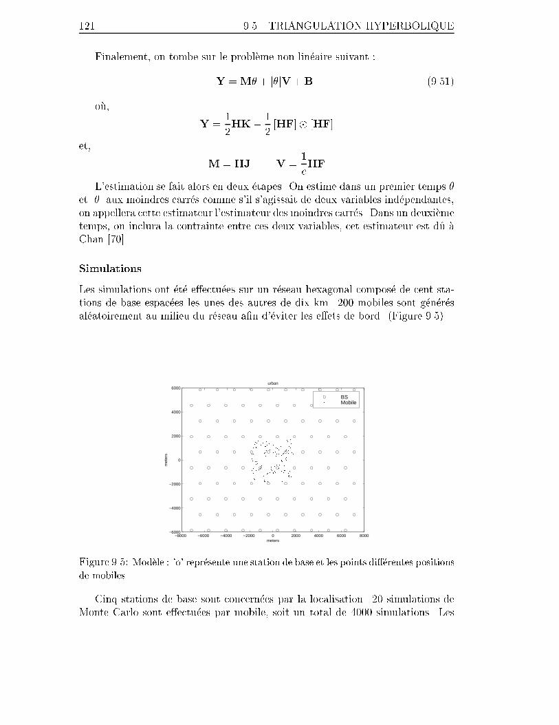
121 9.5. TRIANGULATION HYPERBOLIQUE
Finalement, on tombe sur le probl�eme non lin�eaire suivant :
Y =M� + j�jV +B1 (9.51)
o�u,
Y =1
2HK� 1
2[HF]� [HF]
et,
M = HJ V =1
cHF
L'estimation se fait alors en deux �etapes. On estime dans un premier temps �
et j�j aux moindres carr�es comme s'il s'agissait de deux variables ind�ependantes,
on appellera cette estimateur l'estimateur des moindres carr�es. Dans un deuxi�eme
temps, on inclura la contrainte entre ces deux variables, cet estimateur est du �a
Chan [70].
Simulations
Les simulations ont �et�e e�ectu�ees sur un r�eseau hexagonal compos�e de cent sta-
tions de base espac�ees les unes des autres de dix km. 200 mobiles sont g�en�er�es
al�eatoirement au milieu du r�eseau a�n d'�eviter les e�ets de bord. (Figure 9.5).
−8000 −6000 −4000 −2000 0 2000 4000 6000 8000−6000
−4000
−2000
0
2000
4000
6000
meters
met
ers
urban
BSMobile
Figure 9.5: Mod�ele : 'o' repr�esente une station de base et les points di��erentes positions
de mobiles.
Cinq stations de base sont concern�ees par la localisation. 20 simulations de
Monte Carlo sont e�ectu�ees par mobile, soit un total de 4000 simulations. Les
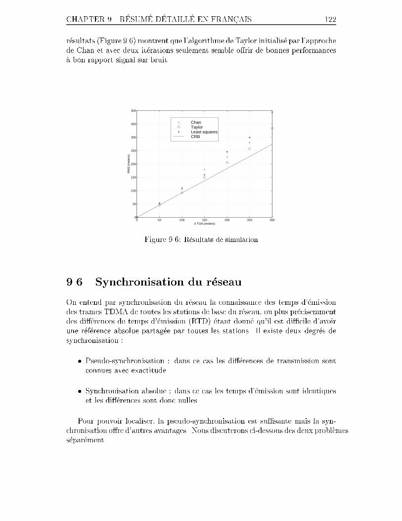
CHAPTER 9. R�ESUM�E D�ETAILL�E EN FRANC�AIS 122
r�esultats (Figure 9.6) montrent que l'algorithme de Taylor initialis�e par l'approche
de Chan et avec deux it�erations seulement semble o�rir de bonnes performances
�a bon rapport signal sur bruit.
0 50 100 150 200 250 3000
50
100
150
200
250
300
350
400
σ TOA (meters)
RM
S (
met
ers)
ChanTaylorLeast squaresCRB
Figure 9.6: R�esultats de simulation
9.6 Synchronisation du r�eseau
On entend par synchronisation du r�eseau la connaissance des temps d'�emission
des trames TDMA de toutes les stations de base du r�eseau, ou plus pr�ecisemment
des di��erences de temps d'�emission (RTD) �etant donn�e qu'il est di�cile d'avoir
une r�ef�erence absolue partag�ee par toutes les stations. Il existe deux degr�es de
synchronisation :
� Pseudo-synchronisation : dans ce cas les di��erences de transmission sont
connues avec exactitude.
� Synchronisation absolue : dans ce cas les temps d'�emission sont identiques
et les di��erences sont donc nulles.
Pour pouvoir localiser, la pseudo-synchronisation est su�sante mais la syn-
chronisation o�re d'autres avantages. Nous discuterons ci-dessous des deux probl�emes
s�epar�ement.
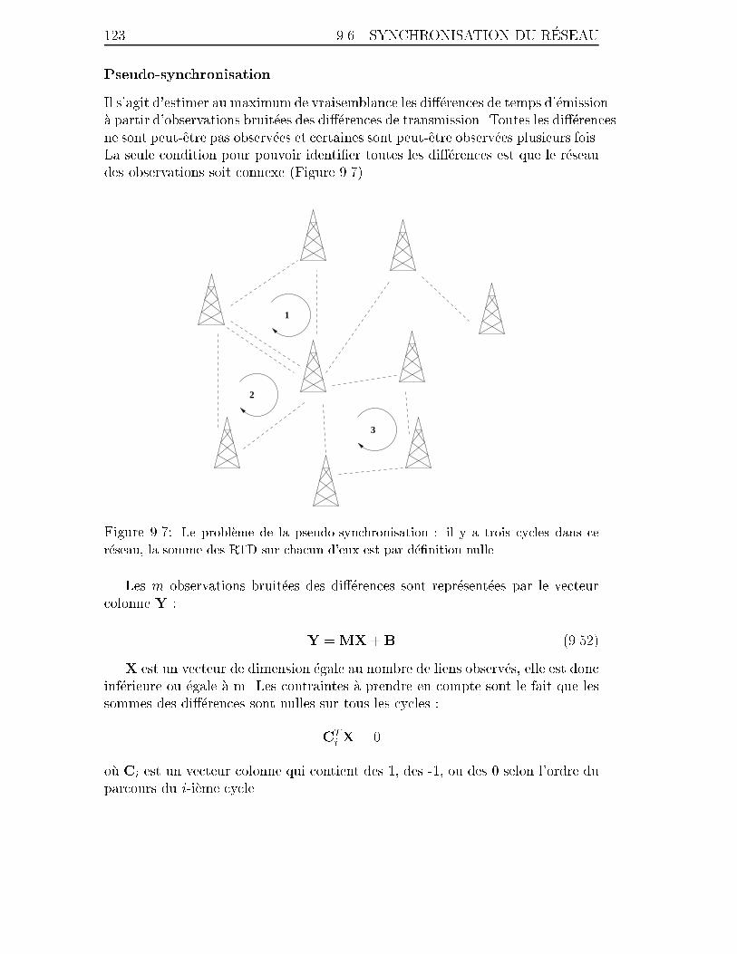
123 9.6. SYNCHRONISATION DU R�ESEAU
Pseudo-synchronisation
Il s'agit d'estimer au maximum de vraisemblance les di��erences de temps d'�emission
�a partir d'observations bruit�ees des di��erences de transmission. Toutes les di��erences
ne sont peut-etre pas observ�ees et certaines sont peut-etre observ�ees plusieurs fois.
La seule condition pour pouvoir identi�er toutes les di��erences est que le r�eseau
des observations soit connexe (Figure 9.7).
1
2
3
Figure 9.7: Le probl�eme de la pseudo-synchronisation : il y a trois cycles dans ce
r�eseau, la somme des RTD sur chacun d'eux est par d�e�nition nulle.
Les m observations bruit�ees des di��erences sont repr�esent�ees par le vecteur
colonne Y :
Y =MX+B (9.52)
X est un vecteur de dimension �egale au nombre de liens observ�es, elle est donc
inf�erieure ou �egale �a m. Les contraintes �a prendre en compte sont le fait que les
sommes des di��erences sont nulles sur tous les cycles :
CT
iX = 0
o�u Ci est un vecteur colonne qui contient des 1, des -1, ou des 0 selon l'ordre du
parcours du i-i�eme cycle.

CHAPTER 9. R�ESUM�E D�ETAILL�E EN FRANC�AIS 124
Le probl�eme �a r�esoudre est celui d'une estimation lin�eaire sous contrainte :
(Y =MX+B
CTX = 0(9.53)
o�u C = [C1 � � �CN ] est de rang plein (cycles ind�ependants). La solution est
donn�ee par :
X =
�I�KC
�CTKC
��1CT
�~X (9.54)
avec K =hMTQ�1M
i�1o�u Q est la matrice de covariance du bruit B.
Synchronisation absolue
Chaque station de base corrige son temps d'�emission en fonction de l'observation
du temps d'arriv�ee de ses voisines :
t0i= ti + �
Pj 6=i pij(tj � ti)P
j 6=i pij(9.55)
pij est un coe�cient de pond�eration. En notant Xn = [t1 � � � tN ]T l'�etat du
r�eseau �a l'�etape n et P la matrice fabriqu�ee �a partir despijPj 6=i
pij, on obtient :
Xn = Xn�1 + �(P� I)Xn�1 = [(1� �)I+ �P]Xn�1 =MXn�1 (9.56)
Soit :
Xn =MnX0 (9.57)
Notons que P n'est pas forc�ement sym�etrique (toutes les stations de base n'ont
pas le meme nombre de voisines). On peut d�emontrer que ce syst�eme converge
en probabilit�e vers l'�etat synchrone :
limn!1
Mnv = �1
o�u v est initialis�e al�eatoirement et � un facteur quelconque.
9.7 Simulations globales
Dans les sections pr�ec�edentes, nous avons trait�e s�epar�ement le probl�eme de l'estimation
du temps d'arriv�ee et celui de la fusion de donn�ees. Nous nous proposons ici
d'utiliser les deux �etapes cons�ecutivement dans des environnements concrets pour
pouvoir en d�eduire les performances que l'on peut attendre d'un tel syst�eme de
localisation.
125 9.7. SIMULATIONS GLOBALES
9.7.1 Mod�ele de canal
Nous examinons ici la mani�ere de g�en�erer une r�eponse impulsionnelle du canal
repr�esent�ee par un �etalement temporel, un nombre d'�echos et pour chaque �echo
son retard, sa puissance moyenne et la distribution de probabilit�e de son ampli-
tude.
On conviendra que chaque �echo r�esulte de la superposition de plusieurs ondes
qui arrivent toutes au meme moment [76, 77] :
E(t) =nXi=1
Ei exp
�j(�0 +
2�
�vt cos�i)
�(9.58)
o�u �i d�esigne l'angle d'incidence de la i-i�eme onde, �0 d�esigne la phase initiale
et v d�esigne la vitesse du mobile. L'amplitude r�esultante est donc la somme des
di��erentes contributions. Si l'�echo correspondant n'est pas un trajet direct, les
phases de ces ondes sont uniformes, l'amplitude est alors gaussienne de moyenne
nulle et le module suit une loi de distribution de Rayleigh. En revanche, lorsqu'il
s'agit d'un trajet direct, les phases ne sont pas tout a fait uniformes et l'amplitude
r�esultante est gaussienne de moyenne non nulle. Son module suit une loi de
distribution de Rice. La corr�elation dans le temps de l'amplitude est donn�ee
par :
R(�) =Z 2�
0p(�) exp
�j2�
�v� cos�
�d� (9.59)
p(�) d�esigne la distribution de probabilit�e angulaire des ondes. Si celles-ci
sont uniformes, on obtient alors le c�el�ebre mod�ele de Jakes :
R(�) = J0(2�
�v�) , �R(f) =
1r1�
�f
fd
�2 (9.60)
avec �R(f) le spectre Doppler et fd = v
�la fr�equence Doppler. Dans nos
simulations, � sera suppos�e gaussien de moyenne constante et d'�ecart-type 0.15
radians. Ce mod�ele correspond au fait que les ondes arrivent concentr�ees dans
un faisceau �etroit. Dans tous les cas de �gure, plus la vitesse est grande plus
l'amplitude tend �a etre moins corr�el�ee dans le temps. La g�en�eration de l'amplitude
sera faite selon la formule (9.58). Si parmi les di��erentes ondes aucune n'est
d�eterministe, on obtient simplement une loi de distribution de Rayleigh. En
revanche si une onde est d�eterministe, la moyenne statistique n'est pas nulle,
et on obtient une loi de distribution de Rice. Il est fr�equent d'utiliser la loi de
distribution de Nakagami pour mod�eliser ces di��erences :
p(r) =2mmr2m�1
�(m)mexp(�m
r2) (9.61)
CHAPTER 9. R�ESUM�E D�ETAILL�E EN FRANC�AIS 126
La variable m re �ete l'importance de la composante d�eterministe : plus m est
grand, plus cette composante est importante. d�esigne la puissance moyenne de
l'�echo. Nous avons trois possibilit�es :
� m = 1 : distribution de Rayleigh.
� m > 1 : approximation de la loi de Rice.
� m =1 : distribution de Dirac, l'�echo est purement d�eterministe.
La g�er�eration des ondes s'e�ectue grace aux deux relations suivantes [77] :
A1 =
vuut
s1� 1
m
�2 =
n(1�
s1� 1
m)
avec A1 l'amplitude de la composante d�eterministe et �2 la puissance moyenne
des autres ondes.
Plusieurs pro�ls ont �et�e s�electionn�es :
� Urbain (en indoor �a 3km/h et outdoor �a 3 and 50 km/h) : zones denses,
grands immeubles et centre ville.
� Banlieue outdoor (�a 3 et 50 km/h) : zones r�esidentielles, banlieues et vil-
lages.
� Rural (�a 3 et 100 km/h) : zones inhabit�ees, autoroutes, champs et forets.
La di��erence majeure entre le pro�l urbain et les autres pro�ls r�eside dans
l'existence du trajet direct. Il n'y a pas de trajet direct dans les zones urbaines
alors qu'un puissant trajet direct existe dans les autres pro�ls.
Ces hypoth�eses sont bas�ees sur le mod�ele de canal �etabli lors des r�eunions du
comit�e de normalisation am�ericain T1P1.5 [80].
9.7.2 Estimation du temps d'arriv�ee
Le mod�ele de Greenstein est choisi pour g�en�erer un �etalement temporel et les
param�etres des di��erentes constantes sont �x�es pour chaque pro�l. La g�en�eration
des puissances moyennes des di��erents �echos est exponentiellement d�ecroissante
pour le pro�l urbain. Les valeurs des di��erents param�etres �gurent dans la Ta-
ble 9.1.
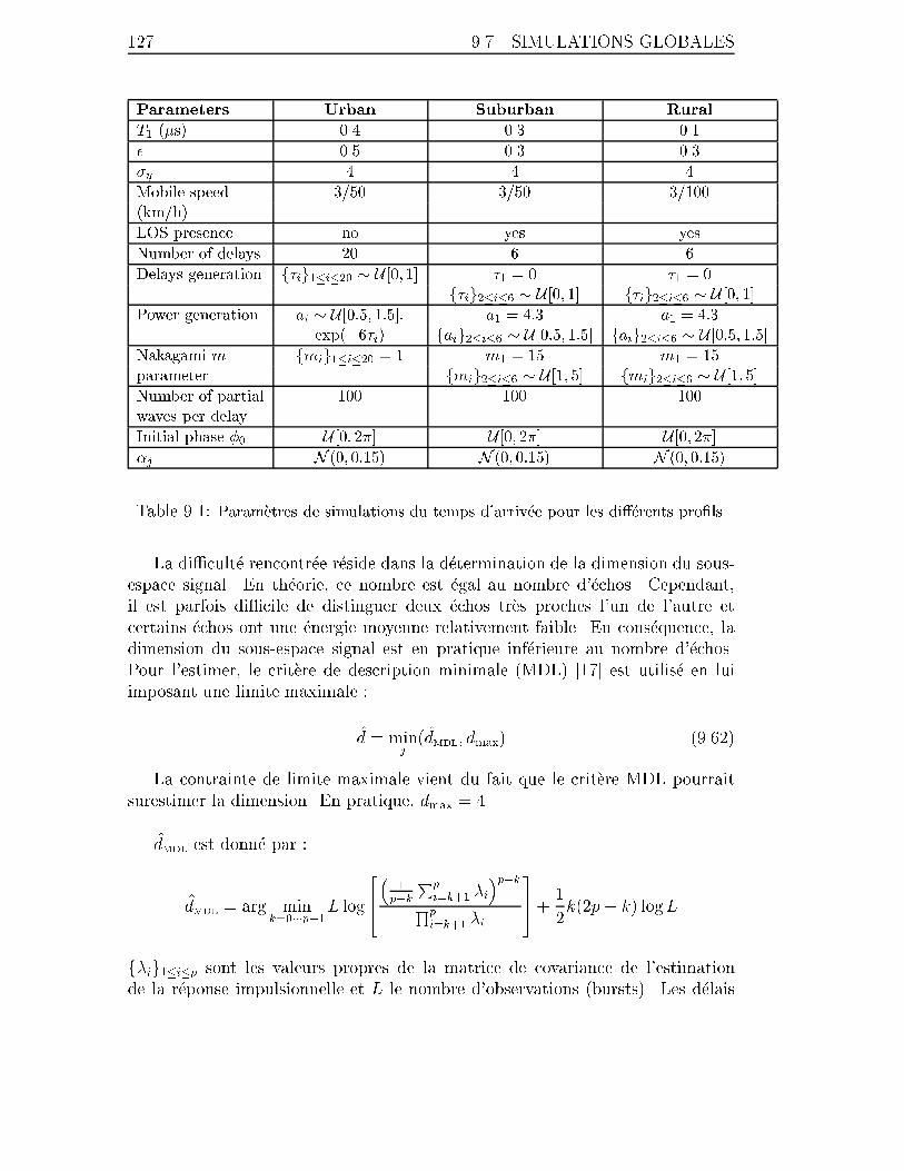
127 9.7. SIMULATIONS GLOBALES
Parameters Urban Suburban Rural
T1 (�s) 0.4 0.3 0.1
� 0.5 0.3 0.3
�y 4 4 4
Mobile speed 3/50 3/50 3/100
(km/h)
LOS presence no yes yes
Number of delays 20 6 6
Delays generation f�ig1�i�20 � U [0; 1] �1 = 0 �1 = 0
f�ig2�i�6 � U [0; 1] f�ig2�i�6 � U [0; 1]
Power generation ai � U [0:5; 1:5]: a1 = 4:3 a1 = 4:3
exp(�6�i) faig2�i�6 � U [0:5; 1:5] faig2�i�6 � U [0:5; 1:5]
Nakagami m fmig1�i�20 = 1 m1 = 15 m1 = 15
parameter fmig2�i�6 � U [1; 5] fmig2�i�6 � U [1; 5]
Number of partial 100 100 100
waves per delay
Initial phase �0 U [0; 2�] U [0; 2�] U [0; 2�]
�j N (0; 0:15) N (0; 0:15) N (0; 0:15)
Table 9.1: Param�etres de simulations du temps d'arriv�ee pour les di��erents pro�ls.
La di�cult�e rencontr�ee r�eside dans la d�etermination de la dimension du sous-
espace signal. En th�eorie, ce nombre est �egal au nombre d'�echos. Cependant,
il est parfois di�cile de distinguer deux �echos tr�es proches l'un de l'autre et
certains �echos ont une �energie moyenne relativement faible. En cons�equence, la
dimension du sous-espace signal est en pratique inf�erieure au nombre d'�echos.
Pour l'estimer, le crit�ere de description minimale (MDL) [17] est utilis�e en lui
imposant une limite maximale :
d = minj(dMDL; dmax) (9.62)
La contrainte de limite maximale vient du fait que le crit�ere MDL pourrait
surestimer la dimension. En pratique, dmax = 4.
dMDL est donn�e par :
dMDL = arg mink=0���p�1
L log
264�
1p�k
Pp
i=k+1 �i�p�k
Qp
i=k+1 �i
375+ 1
2k(2p� k) logL
f�ig1�i�p sont les valeurs propres de la matrice de covariance de l'estimation
de la r�eponse impulsionnelle et L le nombre d'observations (bursts). Les d�elais

CHAPTER 9. R�ESUM�E D�ETAILL�E EN FRANC�AIS 128
sont suppos�es d�ecorr�el�es entre eux. On utilisera Root MUSIC comme estima-
teur du temps d'arriv�ee. Dans la table 9.2, les r�esultats des simulations sont
pr�esent�es �a 10 dB. Les r�esultats sont pr�esent�es en terme de la racine de l'erreur
quadratique moyenne des 90% meilleurs r�esultats. La raison �a cela est que cer-
tains mauvais r�esultats d�egradent cette erreur et il est possible de les corriger
en prenant l'information de l'avance en temps (i.e. la position de la s�equence
d'apprentissage).
20 bursts de synchronisation sont utilis�es. Les simulations montrent claire-
ment que Root MUSIC est sup�erieur au simple �ltrage adapt�e (Table 9.2).
Pro�les Root MUSIC Matched �lter
SNR 0 dB 10 dB 1 dB 0 dB 10 dB 1 dB
Urban 3 km/h 311 231 210 323 323 323
Urban 50 km/h 156 135 134 294 294 294
Suburban 3 km/h 26 20 19 76 74 74
Suburban 50 km/h 10 6 4 47 47 47
Rural 3 km/h 18 16 12 60 58 58
Rural 100 km/h 5 3 3 44 44 44
Table 9.2: Racine de l'erreur quadratique moyenne (en m�etres) pour les 90% meilleurs
r�esultats en utilisant 20 bursts de synchronisation.
Les r�esultats montrent que l'estimation du temps d'arriv�ee d�epend l�eg�erement
du rapport signal sur bruit. Le probl�eme majeur est bien le trajet multiple. Meme
dans un environnement sans bruit (rapport signal sur bruit in�ni) l'erreur n'est
pas nulle.
9.7.3 Estimation de la position
Cette section pr�esente les simulations globales dans un r�eseau hexagonal parfait
avec des antennes omnidirectionnelles. La distance minimale entre les stations de
base varie selon l'environnement. Nous avons choisi un motif de r�eutilisation de
7 stations de base. Nous avons pris le mod�ele de propagation d'Okumura-Hata.
Les param�etres D, Lp, et l'�ecart-type de l'�evanouissement ainsi que les autres
param�etres sont donn�es dans la Table 9.3. Les budgets de puissance montant et
descendant sont suppos�es etre �equilibr�es. Nous avons choisi le front montant. La
sensibilit�e de la station de base d�etermine le niveau du bruit, elle est �x�ee �a -118
dBm.
Par souci de simpli�cation, les interf�erences sont suppos�ees gaussiennes (ap-
proximation AWGN). La vitesse est prise en compte pour la g�en�eration des am-
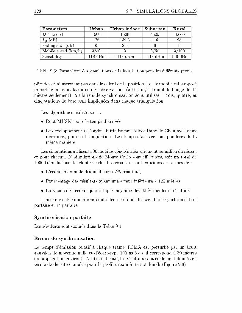
129 9.7. SIMULATIONS GLOBALES
Parameters Urban Urban indoor Suburban Rural
D (meters) 1500 1500 4500 10000
Lp (dB) 126 139.5 116 98
Fading std. (dB) 6 8.5 6 6
Mobile speed (km/h) 3/50 3 3/50 3/100
Sensibility -118 dBm -118 dBm -118 dBm -118 dBm
Table 9.3: Param�etres des simulations de la localisation pour les di��erents pro�ls.
plitudes et n'intervient pas dans le calcul de la position, i.e. le mobile est suppos�e
immobile pendant la dur�ee des observations (�a 50 km/h le mobile bouge de 14
m�etres seulement). 20 bursts de synchronisation sont utilis�es. Trois, quatre, et
cinq stations de base sont impliqu�ees dans chaque triangulation.
Les algorithmes utilis�es sont :
� Root MUSIC pour le temps d'arriv�ee.
� Le d�eveloppement de Taylor, initialis�e par l'algorithme de Chan avec deux
it�erations, pour la triangulation. Les temps d'arriv�ee sont pond�er�es de la
meme mani�ere.
Les simulations utilisent 500 mobiles g�en�er�es al�eatoirement au milieu du r�eseau
et pour chacun, 20 simulations de Monte Carlo sont e�ectu�ees, soit un total de
10000 simulations de Monte Carlo. Les r�esultats sont exprim�es en termes de :
� L'erreur maximale des meilleurs 67% r�esultats,
� Pourcentage des r�esultats ayant une erreur inf�erieure �a 125 m�etres,
� La racine de l'erreur quadratique moyenne des 90 % meilleurs r�esultats.
Deux s�eries de simulations sont e�ectu�ees dans les cas d'une synchronisation
parfaite et imparfaite.
Synchronisation parfaite
Les r�esultats sont donn�es dans la Table 9.4.
Erreur de synchronisation
Le temps d'�emission relatif �a chaque trame TDMA est perturb�e par un bruit
gaussien de moyenne nulle et d'�ecart-type 100 ns (ce qui correspond �a 30 m�etres
de propagation environ). A titre indicatif, les r�esultats sont �egalement donn�es en
terme de densit�e cumul�ee pour le pro�l urbain �a 3 et 50 km/h (Figure 9.8).
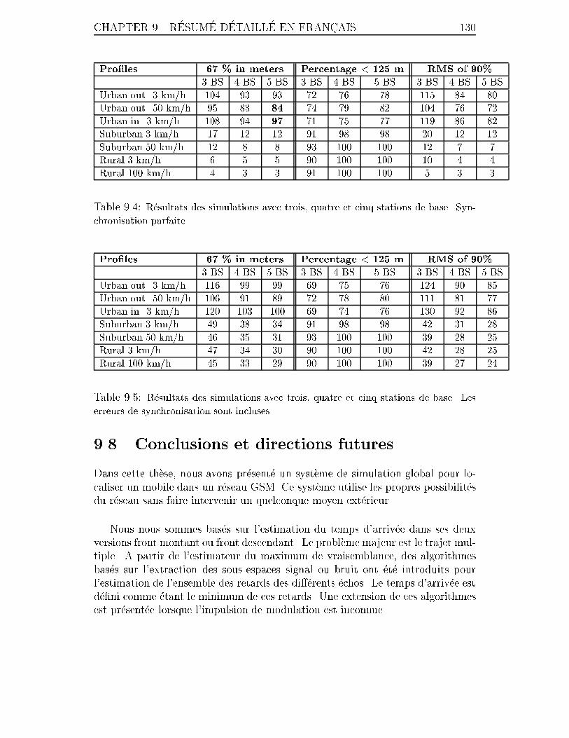
CHAPTER 9. R�ESUM�E D�ETAILL�E EN FRANC�AIS 130
Pro�les 67 % in meters Percentage < 125 m RMS of 90%
3 BS 4 BS 5 BS 3 BS 4 BS 5 BS 3 BS 4 BS 5 BS
Urban out. 3 km/h 104 93 93 72 76 78 115 84 80
Urban out. 50 km/h 95 83 84 74 79 82 104 76 72
Urban in. 3 km/h 108 94 97 71 75 77 119 86 82
Suburban 3 km/h 17 12 12 91 98 98 20 12 12
Suburban 50 km/h 12 8 8 93 100 100 12 7 7
Rural 3 km/h 6 5 5 90 100 100 10 4 4
Rural 100 km/h 4 3 3 91 100 100 5 3 3
Table 9.4: R�esultats des simulations avec trois, quatre et cinq stations de base. Syn-
chronisation parfaite.
Pro�les 67 % in meters Percentage < 125 m RMS of 90%
3 BS 4 BS 5 BS 3 BS 4 BS 5 BS 3 BS 4 BS 5 BS
Urban out. 3 km/h 116 99 99 69 75 76 124 90 85
Urban out. 50 km/h 106 91 89 72 78 80 111 81 77
Urban in. 3 km/h 120 103 100 69 74 76 130 92 86
Suburban 3 km/h 49 38 34 91 98 98 42 31 28
Suburban 50 km/h 46 35 31 93 100 100 39 28 25
Rural 3 km/h 47 34 30 90 100 100 42 28 25
Rural 100 km/h 45 33 29 90 100 100 39 27 24
Table 9.5: R�esultats des simulations avec trois, quatre et cinq stations de base. Les
erreurs de synchronisation sont incluses.
9.8 Conclusions et directions futures
Dans cette th�ese, nous avons pr�esent�e un syst�eme de simulation global pour lo-
caliser un mobile dans un r�eseau GSM. Ce syst�eme utilise les propres possibilit�es
du r�eseau sans faire intervenir un quelconque moyen ext�erieur.
Nous nous sommes bas�es sur l'estimation du temps d'arriv�ee dans ses deux
versions front montant ou front descendant. Le probl�eme majeur est le trajet mul-
tiple. A partir de l'estimateur du maximum de vraisemblance, des algorithmes
bas�es sur l'extraction des sous-espaces signal ou bruit ont �et�e introduits pour
l'estimation de l'ensemble des retards des di��erents �echos. Le temps d'arriv�ee est
d�e�ni comme �etant le minimum de ces retards. Une extension de ces algorithmes
est pr�esent�ee lorsque l'impulsion de modulation est inconnue.
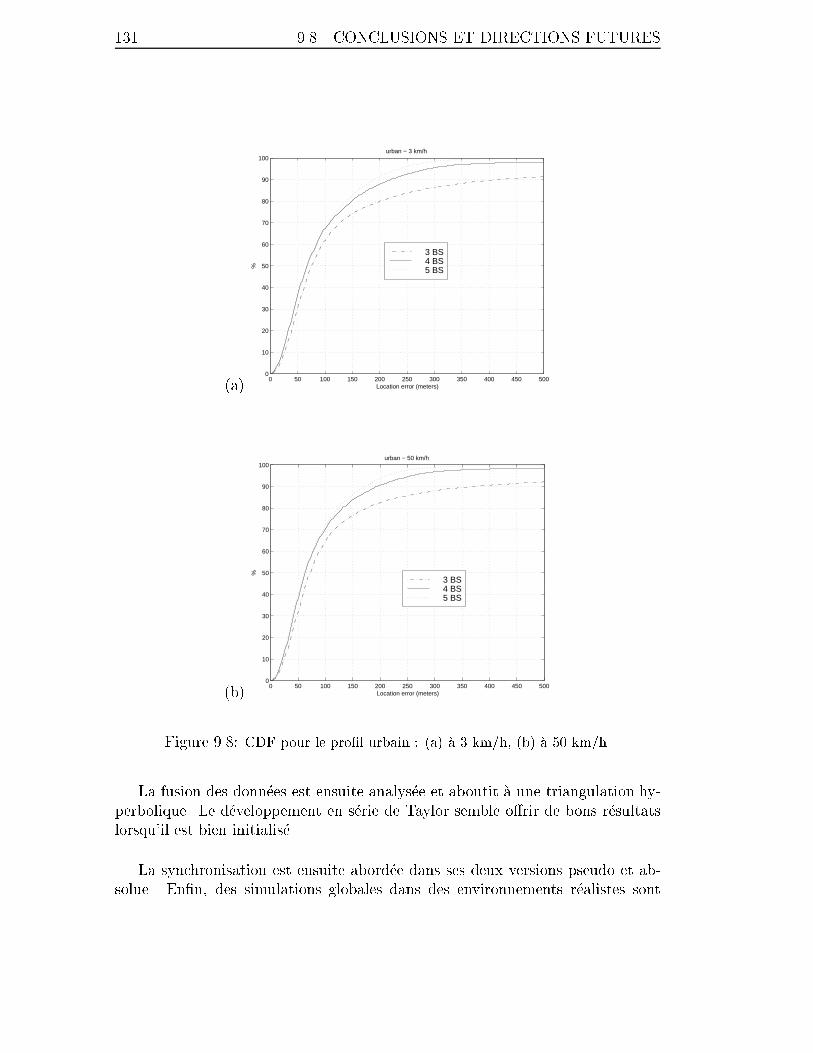
131 9.8. CONCLUSIONS ET DIRECTIONS FUTURES
(a)0 50 100 150 200 250 300 350 400 450 500
0
10
20
30
40
50
60
70
80
90
100
Location error (meters)
%
urban − 3 km/h
3 BS4 BS5 BS
(b)0 50 100 150 200 250 300 350 400 450 500
0
10
20
30
40
50
60
70
80
90
100
Location error (meters)
%
urban − 50 km/h
3 BS4 BS5 BS
Figure 9.8: CDF pour le pro�l urbain : (a) �a 3 km/h, (b) �a 50 km/h.
La fusion des donn�ees est ensuite analys�ee et aboutit �a une triangulation hy-
perbolique. Le d�eveloppement en s�erie de Taylor semble o�rir de bons r�esultats
lorsqu'il est bien initialis�e.
La synchronisation est ensuite abord�ee dans ses deux versions pseudo et ab-
solue. En�n, des simulations globales dans des environnements r�ealistes sont

CHAPTER 9. R�ESUM�E D�ETAILL�E EN FRANC�AIS 132
pr�esent�ees. Les r�esultats semblent encourageants.
Les sujets non abord�es ou �a compl�eter sont les suivants :
Echos di�us
Nous n'avons consid�er�e que les �echos discrets ayant un retard bien d�e�ni. Une
extension possible serait le cas des �echos di�us o�u les ondes arrivent autour d'une
valeur moyenne. Le mod�ele de la r�eponse impulsionnelle du canal est modi��e :
hj(t) =dX
i=1
KiXk=1
sijka(t� �i � ~�ik) 1 � j � L (9.63)
Deux approches sont possibles :
� D�eveloppement en s�erie de Taylor [82, 83].
� Estimation conjointe du retard moyen et de l'�ecart-type autour de la moyenne.
[84{86].
Borne de Cramer-Rao dans le cas d'un impulsion inconnue
Nous n'avons pas calcul�e cette borne. Sa valeur pourrait etre utile pour �evaluer
les r�esultats des algorithmes qui estiment conjointement l'impulsion et les retards.
Pond�eration optimale des temps d'arriv�ee
Nous n'avons pas pond�er�e les temps d'arriv�ee lors de la triangulation. Il est en
e�et di�cile de trouver de telles valeurs. On pourrait �eventuellement se contenter
de valeurs empiriques en fonction du rapport signal-sur-bruit ou de l'�etalement
temporel.
Syst�emes CDMA - UMTS
La localisation est requise pour les futurs standards. Ces standards, comme
l'UMTS (Universal Mobile Telecommunications System), seront bas�es sur la tech-
nologie �a r�epartition en codes (CDMA).
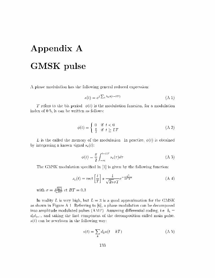
Appendix A
GMSK pulse
A phase modulation has the following general reduced expression:
s(t) = ejP
kbk�(t�kT ) (A.1)
T refers to the bit period. �(t) is the modulation function, for a modulation
index of 0.5, it can be written as follows:
�(t) =
(0 if t < 0�
2if t � LT
(A.2)
L is the called the memory of the modulation. In practice, �(t) is obtained
by integrating a known signal se(t):
�(t) =�
2
Zt�LT
�1se(�)d� (A.3)
The GMSK modulation speci�ed in [1] is given by the following function:
se(t) = rect
�t
T
�?
1p2��T
e�t2
2�2T2 (A.4)
with � =pln 2
2�BTet BT = 0:3.
In reality L is very high, but L = 3 is a good approximation for the GMSK
as shown in Figure A.1. Referring to [6], a phase modulation can be decomposed
into amplitude modulated pulses (AMP). Assuming di�erential coding, i.e. bi =
didi�1, and taking the �rst component of the decomposition called main pulse,
s(t) can be rewritten in the following way:
s(t) =Xk
dka(t� kT ) (A.5)
133

APPENDIX A. GMSK PULSE 134
0 0.5 1 1.5 2 2.5 30
0.1
0.2
0.3
0.4
0.5
0.6
0.7
0.8
0.9
1Phase variation in the GMSK modulation
Bit time
Nor
mal
ized
Pha
se(*
2/π)
Figure A.1: The modulation function in the GMSK.
with,
a(t) = e�j�t
2T
L�1Yi=0
sin[�(t+ iT )] cos[�(t+ (i� L)T )] (A.6)
Other components appear to be negligible; the second component is given by:
b(t) =a(t)a(t + 2T )
a(t + T )
which has an energy 24.35 dB lower than the �rst pulse. The main pulse a(t)
and its secondary pulse are shown in Figure A.2.
a(t) represents the main pulse. In the GMSK modulation, this pulse con-
centrates about 99.6% of the modulation power. In other words, it is a good
approximation to state that the GMSK modulation is linear. The GMSK pulse
has a length of four bit periods, but since it is �ltered to match the 200 kHz
bandwidth, its length may exceed eight bit periods.
Figure A.3 shows the main pulse normalized spectrum.
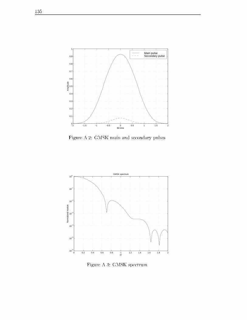
135
−2 −1.5 −1 −0.5 0 0.5 1 1.5 20
0.1
0.2
0.3
0.4
0.5
0.6
0.7
0.8
0.9
1
Bit time
Am
plitu
de
Main pulseSecondary pulse
Figure A.2: GMSK main and secondary pulses.
0 0.2 0.4 0.6 0.8 1 1.2 1.4 1.6 1.8 210
−6
10−5
10−4
10−3
10−2
10−1
100
fT
Nor
mal
ized
mod
ule
GMSK spectrum
Figure A.3: GMSK spectrum.

APPENDIX A. GMSK PULSE 136
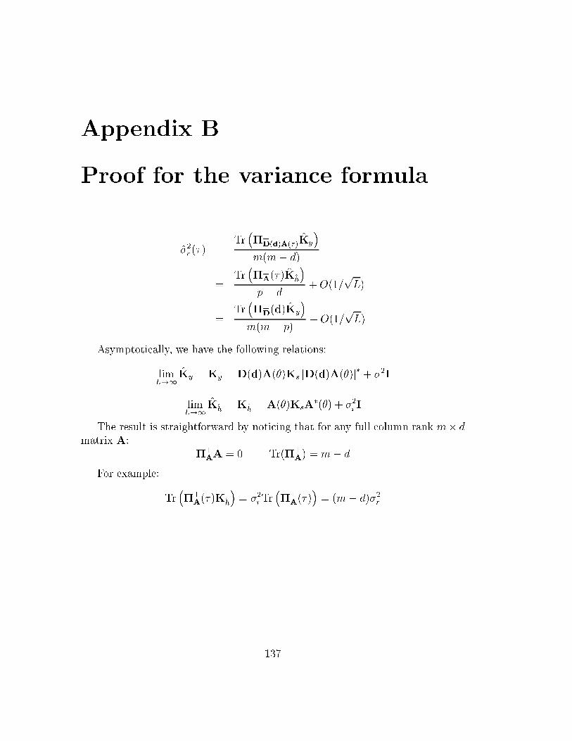
Appendix B
Proof for the variance formula
�2r(�) =
Tr��?D(d)A(�)Ky
�m(m� d)
=Tr��?A(�)K
h
�p� d
+O(1=pL)
=Tr��?D(d)Ky
�m(m� p)
+O(1=pL)
Asymptotically, we have the following relations:
limL!1
Ky = Ky = D(d)A(�)Ks [D(d)A(�)]�+ �2I
limL!1
Kh= K
h= A(�)KsA
�(�) + �2rI
The result is straightforward by noticing that for any full column rank m� dmatrix A:
�?AA = 0 Tr(�?
A) = m� d
For example:
Tr��?A(�)K
h
�= �2
rTr��?A(�)�= (m� d)�2
r
137

APPENDIX B. PROOF FOR THE VARIANCE FORMULA 138
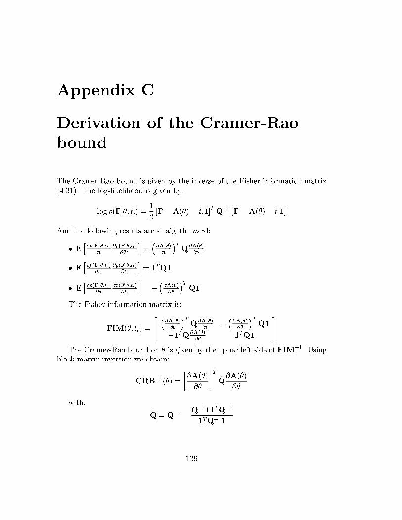
Appendix C
Derivation of the Cramer-Rao
bound
The Cramer-Rao bound is given by the inverse of the Fisher information matrix
(4.31). The log-likelihood is given by:
log p(Fj�; tr) =1
2[F�A(�)� tr1]
TQ�1 [F�A(�)� tr1]
And the following results are straightforward:
� Eh@p(Fj�;tr)
@�
@p(Fj�;tr)@�T
i=�@A(�)
@�
�TQ@A(�)
@�
� Eh@p(Fj�;tr)
@tr
@p(Fj�;tr)@tr
i= 1TQ1
� Eh@p(Fj�;tr)
@�
@p(Fj�;tr)@tr
i= �
�@A(�)
@�
�TQ1
The Fisher information matrix is:
FIM(�; tr) =
24�@A(�)
@�
�TQ@A(�)
@���@A(�)
@�
�TQ1
�1TQ@A(�)
@�1TQ1
35
The Cramer-Rao bound on � is given by the upper left side of FIM�1. Using
block matrix inversion we obtain:
CRB�1(�) =
"@A(�)
@�
#T~Q@A(�)
@�
with:
~Q = Q�1 � Q�111TQ�1
1TQ�11
139

APPENDIX C. DERIVATION OF THE CRAMER-RAO BOUND 140

Appendix D
Mathematical notations
Ay = (A�A)�1A� Moore-Penrose pseudo-inverse of A
A � B matrix comparison , (8x; x�Ax � x�Bx)
AT transpose of A
Ac conjugate of A
A� transpose conjugate of A
�A = AAy projection onto the range space of A
�?A= I��A projection onto the null space of A
A�B Schur product of A and B, i.e. the element by element product
? convolution operator
AB Kronecker product of A and B
Tr(A) trace of A
kAk2 = Tr(A�A) Frobenius norm of A
jAj determinant of A
Vec(A) the column vector made by stacking the columns of A
Re(:) real part
Im(:) imaginary part
E[:] mathematical expectation
�ij Kronecker symbol, 1 if i = j, 0 otherwise
�(t) Dirac delta fucntion
I identity matrix with the appropriate dimension
J anti-identity matrix with the appropriate dimension
j2 = �1I0 and J0 the modi�ed and normal Bessel function of order 0
� the gamma function
N (m; �2) normal variable with mean m and variance �2
U [a; b] uniform variable on [a; b]
141

APPENDIX D. MATHEMATICAL NOTATIONS 142

Appendix E
Abbreviations
AMP Amplitude Modulated Pulse
AWGN Additive White Gaussian Noise
BCCH Broadcast Common CHannel
BER Bit Error Rate
BSIC Base Station Identity Code
BSC Base Station Controller
BSS Base Station Subsystem
BS Base Station
CDMA Code Division Multiple Access
CRB Cramer-Rao Bound
DoA Direction of Arrival
DToA Di�erence Times of Arrival
DTX Discontinuous Transmission
ETSI European Telecommunications Standards Institute
ESPRIT Estimation of Signal Parameters via Rotational Invariance Techniques
FCCH Frequency Correction Channel
FDD Frequency Division Duplex
FDMA Frequency Division Multiple Access
FFT Fast Fourier Transform
FH Frequency Hopping
FN Frame Number
GDoP Geometric Dilution of Precision
GMSK Gaussian Minimum Shift Keying
GSM Global System for Mobile communications
HLR Home Location Register
HO HandOver
IQML Iterative Quadratic Maximum Likelihood
ISI Inter Symbol Interference
JADE Joint Angle and Delay Estimation
LAC Location Area Code
143
APPENDIX E. ABBREVIATIONS 144
LMU Location Mobile Unit
MLC Mobile Location Center
MSC Mobile services Switching Center
MSK Minimum Shift Keying
MUSIC MUltiple SIgnal Characterization
PLMN Public Land Mobile Network
PSTN Public Switched Telephone Network
RACH Random Access CHannel
RTD Real Times Di�erence
SCH Synchronization CHannel
SIM Subscriber Identity Member
SMS Short Message Service
TA Timing Advance
TDMA Time Division Multiple Access
ToA Time of Arrival
UMTS Universal Mobile Telecommunications System
ULA Uniform Linear Array
VLR Visitor Location Register
WSF Weight Subspace Fitting
Bibliography
[1] European Telecommunication Standards Institute, \Digital cellular telecom-
munication system (phase 2+)," 1997.
[2] M. Hata, \Empirical formula for propagation loss in land mobile radio ser-
vice," IEEE Trans. Vehicular Technology, vol. 29, no. 3, pp. 317{325, August
1980.
[3] L. Yuanqing, \A theoretical formulation for the distribution density of mul-
tipath delay spread in a land mobile radio environment," IEEE Trans. Ve-
hicular Technology, vol. 43, no. 2, pp. 379{388, May 1994.
[4] L. J. Greenstein, V. Erceg, Y. S. Yeh, and M. V. Clark, \A new path-
gain/delay-spread propagation model for digital cellular channels," IEEE
Trans. Vehicular Technology, vol. 46, no. 2, pp. 477{485, May 1997.
[5] M. Mouly and M.-B. Pautet, The GSM system for mobile communications.
Europe Media, 1992.
[6] P. A. Laurent, \Exact and approximate construction of digital phase mod-
ulations by superposition of amplitude modulated pulses (AMP)," IEEE
Trans. Communications, vol. 34, no. 2, pp. 150{160, February 1986.
[7] G. J. Bierman, Factorization methods for discrete sequential estimation. Aca-
demic Press, 1977.
[8] G. D. Forney, \Maximum-likelihood sequence estimation of digital sequences
in the presence of intersymbol interference," IEEE Trans. Information The-
ory, vol. 18, no. 3, pp. 363{378, May 1972.
[9] M. Hellebrandt, R. Mathar, and M. Scheibenbogen, \Estimating position
and velocity of mobiles in a cellular radio network," IEEE Trans. Vehicular
Technology, vol. 46, no. 1, pp. 65{71, February 1997.
[10] L. Breiman, Classi�cation and regression trees. Monterey, California:
Wadsworth, 1984.
145
BIBLIOGRAPHY 146
[11] H. Krim and M. Viberg, \Two decades of array signal processing research,"
IEEE Signal Processing Magazine, pp. 67{94, July 1996.
[12] M. Wax and A. Leshem, \Joint estimation of time delays and directions
of arrival of multiple re ections of a known signal," IEEE Trans. Signal
Processing, vol. 45, no. 10, pp. 2477{2484, October 1997.
[13] A.-J. Van Der Veen, M. C. Vanderveen, and A. Paulraj, \Joint angle and
delay estimation using shift-invariance techniques," IEEE Trans. Signal Pro-
cessing, vol. 46, no. 2, pp. 405{418, February 1998.
[14] G. G. Raleigh and T. Boros, \Joint space-time parameter estimation for
wireless communication channels," IEEE Trans. Signal Processing, vol. 46,
no. 5, pp. 1333{1343, May 1998.
[15] A. Zeira and P. M. Schultheiss, \Time delay estimation for closely spaced
echoes," Proc. ICASSP, pp. 2763{2766, 1990.
[16] M. Wax, T.-J. Shan, and T. Kailath, \Spatio-temporal spectral analysis by
eigenstructure methods," IEEE Trans. Acoust., Speech, Signal Processing,
vol. 37, no. 8, pp. 1190{1196, August 1984.
[17] M. Wax and T. Kailath, \Detection of signals by information theoretic crite-
ria," IEEE Trans. Acoust., Speech, Signal Processing, vol. 33, no. 2, pp. 387{
392, April 1985.
[18] Y. Q. Yin and P. R. Krishnaiah, \On some nonparametric methods for
detection of the number of signals," IEEE Trans. Acoust., Speech, Signal
Processing, vol. 35, no. 11, pp. 1533{1538, November 1987.
[19] M. Wax and I. Ziskind, \Detection of the number of coherent signals by the
MDL principle," IEEE Trans. Acoust., Speech, Signal Processing, vol. 37,
no. 8, pp. 1190{1196, August 1989.
[20] K. M. Wong, Q.-T. Zhang, J. P. Reilly, and P. C. Yip, \On information
theoretic criteria for determining the number of signals in high resolution
array processing," IEEE Trans. Acoust., Speech, Signal Processing, vol. 38,
no. 11, pp. 1959{1971, November 1990.
[21] H. Lee and F. Li, \An eigenvector technique for detecting the number of emit-
ters in a cluster," IEEE Trans. Signal Processing, vol. 42, no. 9, pp. 2380{
2388, September 1994.
[22] G. Xu, R. H. Roy, and T. Kailath, \Detection of number of sources via
exploitation of centro-symmetry property," IEEE Trans. Signal Processing,
vol. 42, no. 1, pp. 102{112, January 1994.

147 BIBLIOGRAPHY
[23] A. Bruckstein, T.-J. Shan, and T. Kailath, \The resolution of overlap-
ping echos," IEEE Trans. Acoust., Speech, Signal Processing, vol. 33, no. 6,
pp. 1357{1367, December 1985.
[24] M. C. Vanderveen, A.-J. Van Der Veen, and A. Paulraj, \Estimation of mul-
tipath parameters in wireless communications," IEEE Trans. Signal Pro-
cessing, vol. 46, no. 3, pp. 682{690, March 1998.
[25] B. G�oransson and B. Ottersten, \E�cient direction estimation of uncorre-
lated sources using polynomial rooting," Proceedings DSP 97, 1997.
[26] P. Stoica and A. Nehorai, \Performance study of conditional and uncondi-
tional direction-of-arrival estimation," IEEE Trans. Acoust., Speech, Signal
Processing, vol. 38, no. 10, pp. 1783{1795, October 1990.
[27] P. Stoica and A. Nehorai, \MUSIC, maximum likelihood, and Cramer-Rao
bound," IEEE Trans. Acoust., Speech, Signal Processing, vol. 37, no. 5,
pp. 720{741, May 1989.
[28] J. F. B. B�ohme, \Estimation of spectral parameters of correlated signals in
wave�elds," Signal Processing, vol. 11, pp. 329{337, 1986.
[29] Y. Bresler and A. Macovski, \Maximum likelihood estimation of linearly
structured covariance with application to antenna array processing," Proc.
ICASSP, pp. 172{175, 1986.
[30] H. L. Van Trees, Detection, estimation and modulation theory, part I and
III. New York: Wiley, 1971.
[31] D. Starer and A. Nehorai, \Newton algorithms for conditional and uncon-
ditional maximum likelihood estimation of the parameters of exponential
signals in noise," IEEE Trans. Signal Processing, vol. 40, no. 6, pp. 1528{
1534, June 1992.
[32] I. Ziskind and M. Wax, \Maximum likelihood localization of multiple sources
by alternating projection," IEEE Trans. Acoust., Speech, Signal Processing,
vol. 36, no. 10, pp. 1553{1560, October 1988.
[33] M. Feder and E. Weinstein, \Parameter estimation of superimposed signals
using the em algorithm," IEEE Trans. Acoust., Speech, Signal Processing,
vol. 36, no. 4, pp. 477{489, April 1988.
[34] M. I. Miller and D. R. Fuhrmann, \Maximum-Likelihood narrow-band di-
rection �nding and the EM algorithm," IEEE Trans. Acoust., Speech, Signal
Processing, vol. 38, no. 9, pp. 1560{1577, September 1990.
BIBLIOGRAPHY 148
[35] M. Segal, E. Weinstein, and B. R. Musicus, \Estimate-Maximize algorithms
for multichannel time delay and signal estimation," IEEE Trans. Signal Pro-
cessing, vol. 39, no. 1, pp. 1{16, January 1991.
[36] J. Capon, \High-resolution frequency-wavenumber spectrum analysis," Proc.
IEEE, vol. 57, no. 8, pp. 2408{2418, 1969.
[37] B. Friedlander, \A sensitivity analysis of the MUSIC algorithm," IEEE
Trans. Acoust., Speech, Signal Processing, vol. 38, no. 10, pp. 1740{1751,
October 1990.
[38] P. Stoica and A. Nehorai, \Music, maximum likelihood, and Cram�er-Rao
bound: further results and comparisons," IEEE Trans. Acoust., Speech, Sig-
nal Processing, vol. 38, no. 12, pp. 2140{2150, December 1990.
[39] M. Viberg and B. Ottersten, \Sensor array processing based on subspace
�tting," IEEE Trans. Signal Processing, vol. 39, no. 5, pp. 1110{1121, May
1991.
[40] M. Viberg, B. Ottersten, and T. Kailath, \Detection and estimation in sen-
sor arrays using weighted subspace �tting," IEEE Trans. Signal Processing,
vol. 39, no. 11, pp. 2436{2249, November 1991.
[41] B. Ottersten, M. Viberg, and T. Kailath, \Analysis of subspace �tting and
ML techniques for parameter estimation from sensor array data," IEEE
Trans. Signal Processing, vol. 40, no. 3, pp. 590{600, March 1992.
[42] B. Friedlander and A. Weiss, \Eigenstructure methods for direction �nding
with sensor gain and phase uncertainties," Proc. ICASSP, pp. 2681{2684,
1988.
[43] V. C. Soon, L. Tong, H. Y. F., and L. R., \A subspace method for estimating
sensor gains and phases," IEEE Trans. Signal Processing, vol. 42, no. 4,
pp. 1973{1976, April 1994.
[44] V. F. Pisarenko, \The retrieval of harmonics from covariance functions,"
Geophys. J. Roy. Astronom. Soc., pp. 347{366, 1972.
[45] B. D. Rao and K. V. Hari, \Performance analysis of root-Music," IEEE
Trans. Acoust., Speech, Signal Processing, vol. 37, no. 12, pp. 1939{1949,
December 1989.
[46] Y. Bresler and A. Macovski, \Exact maximum likelihood parameter estima-
tion of superimposed exponential signals in noise," IEEE Trans. Acoust.,
Speech, Signal Processing, vol. 34, no. 5, pp. 1081{1089, October 1986.
149 BIBLIOGRAPHY
[47] P. Stoica and K. C. Sharman, \Maximum likelihoodmethods for direction-of-
arrival estimation," IEEE Trans. Acoust., Speech, Signal Processing, vol. 38,
no. 7, pp. 1132{1143, July 1990.
[48] P. Stoica, J. Li, and T. S�oderstr�om, \On the inconsistency of IQML," Signal
Processing, vol. 56, no. 2, pp. 185{190, January 1997.
[49] M. Kristensson, M. Jansson, and B. Ottersten, \Modi�ed IQML and
weighted subspace �tting without eigendecomposition," to appear in Signal
Processing, 1999.
[50] R. Roy and T. Kailath, \ESPRIT - Estimation of signal parameters via
rotational invariance techniques," IEEE Trans. Acoust., Speech, Signal Pro-
cessing, vol. 37, no. 7, pp. 984{995, July 1989.
[51] B. Ottersten, M. Viberg, and T. Kailath, \Performance analysis of the total
least squares ESPRIT algorithm," IEEE Trans. Signal Processing, vol. 39,
no. 5, pp. 1122{1135, May 1991.
[52] A. Eriksson and P. Stoica, \Optimally weighted ESPRIT for direction esti-
mation," Signal Processing, vol. 38, pp. 223{229, 1994.
[53] A. L. Swindlehurst, B. Ottersten, R. Roy, and T. Kailath, \Multiple invari-
ance ESPRIT," IEEE Trans. Signal Processing, vol. 40, no. 4, pp. 867{881,
April 1992.
[54] R. Bachl, \The forward-backward averaging technique applied to TLS-
ESPRIT processing," IEEE Trans. Signal Processing, vol. 43, no. 11,
pp. 2691{2699, November 1995.
[55] M. Jansson, On subspace methods in system identi�cation and sensor array
signal processing. PhD thesis, Royal institute of Technology, Department of
Signals, Sensors and Systems, Stockholm, Sweden, 1997.
[56] A. L. Swindlehurst and T. Kailath, \A performance analysis of subspace-
based methods in the presence of model errors, part I: the MUSIC algo-
rithm," IEEE Trans. Signal Processing, vol. 40, no. 7, pp. 1758{1774, July
1992.
[57] A. L. Swindlehurst and T. Kailath, \A performance analysis of subspace-
based methods in the presence of model errors, part II: multidimensional
algorithms," IEEE Trans. Signal Processing, vol. 41, no. 9, pp. 2882{2890,
September 1993.
[58] M. Jansson, A. L. Swindlehurst, and B. Ottersten, \Weighted subspace �t-
ting for general array error models," IEEE Trans. Signal Processing, vol. 46,
no. 9, pp. 2484{2498, September 1998.
BIBLIOGRAPHY 150
[59] A. Paulraj and T. Kailath, \Direction of arrival estimation by eigenstructure
methods with unknown sensor gains and phases," Proc. ICASSP, pp. 640{
643, 1985.
[60] D. Aszt�ely, Spatial and spatio-temporal processing with antenna arrays in
wireless systems. PhD thesis, Royal institute of Technology, Department of
Signals, Sensors and Systems, Stockholm, Sweden, 1999.
[61] G. G. H. and V. Loan, Matrix computations. Baltimore: Johns Hopkins
University Press, 1990.
[62] G. W. Stewart, \An updating algorithm for subspace tracking," IEEE Trans.
Signal Processing, vol. 40, no. 6, pp. 1535{1541, June 1992.
[63] G. Xu, R. H. Roy, and T. Kailath, \Fast subspace decomposition," IEEE
Trans. Signal Processing, vol. 42, no. 3, pp. 539{551, March 1994.
[64] S. Marcos, Les m�ethodes �a haute r�esolution. Paris: Herm�es, 1998.
[65] B. Yang, \Projection approximation subspace tracking," IEEE Trans. Signal
Processing, vol. 43, no. 1, pp. 95{107, January 1995.
[66] E. D. Kaplan, Understanding GPS, principles and applications. Boston:
Artech House, 1996.
[67] D. J. Torrieri, \Statistical theory of passive location systems," IEEE Trans.
Aeros. Electronic Systems, vol. 20, pp. 183{198, March 1984.
[68] W. H. Foy, \Position-location solutions by Taylor-series estimation," IEEE
Trans. Aeros. Electronic Systems, vol. 12, no. 2, pp. 187{194, March 1976.
[69] M. Wax and T. Kailath, \Optimum localization of multiple sources by pas-
sive arrays," IEEE Trans. Acoust., Speech, Signal Processing, vol. 31, no. 5,
pp. 1210{1218, October 1983.
[70] Y. T. Chan and K. C. Ho, \A simple and e�cient estimator for hyperbolic
location," IEEE Trans. Signal Processing, vol. 42, no. 8, pp. 1905{1915,
August 1994.
[71] L. Le Bris, Allocation de resources radio. PhD thesis, Universit�e Paris VII,
UFR d'informatique, Paris, France, 1999.
[72] M. Gondran and M. Minoux, Graphes et algorithmes. Eyrolles, 1995.
[73] F. R. Gantmacher, Th�eorie des matrices, tomes I et II. Dunod, 1966.
[74] I. S. Gradshteyn and I. M. Ryzhik, Tables of integrals, series, and products.
Academic Press, 1979.
151 BIBLIOGRAPHY
[75] J. C.-I. Chuang, \Autonomous time synchronization among radio ports
in wireless personal communications," IEEE Trans. Vehicular Technology,
vol. 43, no. 1, pp. 27{32, February 1994.
[76] W. R. Braun, \A physical mobile radio channel model," IEEE Trans. Ve-
hicular Technology, vol. 40, no. 2, pp. 472{482, May 1991.
[77] U. Dersch and R. J. R�uegg, \Simulations of the time and frequency selective
outdoor mobile radio channel," IEEE Trans. Vehicular Technology, vol. 42,
no. 3, pp. 338{344, 1993.
[78] M. Nakagami, Them distribution{ a general formula of intensity distribution
of rapid fading, pp. 3{36. New York: Pergamon Press, 1958.
[79] S. Aun Abbas and A. U. Sheikh, \A geometric theory of Nakagami fading
multipath mobile radio channel with physical interpretations," Proc. VTC,
pp. 637{641, 1996.
[80] Ericsson, \Evaluation of positioningmeasurement systems," T1P1.5/98-110,
http://www.t1.org, 1998.
[81] X. Lagrange, P. Godlewski, and S. Tabbane, R�eseaux GSM-DCS. Paris:
Herm�es, 1995.
[82] D. Aszt�ely and B. Ottersten, \The e�ects of local scaterring on direction of
arrival estimation with MUSIC and ESPRIT," Proc. ICASSP, 1998.
[83] D. Aszt�ely and B. Ottersten, \A generalized array manifold model for local
scaterring in wireless communications," Proc. ICASSP, 1997.
[84] T. Trump and B. Ottersten, \Estimation of nominal direction of arrival and
angular spread using an array of sensors," Signal Processing, vol. 50, 1996.
[85] Y. Meng, P. Stoica, and K. M. Wong, \Estimation of the directions of arrival
of spatially dispersed signals in array processing," IEE Proc.-Radar, Sonar
Navig., vol. 143, no. 1, pp. 1{9, February 1996.
[86] M. Bengtsson and B. Ottersten, \Rooting techniques for estimation of an-
gular spread with an antenna array," Proc. VTC, 1996.