Three Essays on

Workforce Scheduling

Inauguraldissertationzur Erlangung des akademischen Grades

eines Doktors der Wirtschaftswissenschaftender Universitat Mannheim

vorgelegt von

Emilio Zamorano de AchaMannheim

Dekan: Prof. Dr. Dieter TruxiusReferent: Prof. Dr. Raik StolletzKorreferent: Prof. Dr. Jens Brunner

Tag der mundlichen Prufung: 22. April 2016

To Christine,

Isabel, and Sebastian

Acknowledgements

It was late summer of 2010, when I embarked on this exciting academicvoyage. Since then, I have been fortunate enough to be accompanied bypeople who stood by me throughout this journey. Their guidance, counsel,and support allowed me to succeed in concluding the projects included inthis dissertation. In the following, few words to express my gratitude.

I would like to extend my appreciation to my supervisor, Prof. Dr. RaikStolletz, for the invaluable advice and support he provided during thelast years. I would also like to thank my co-author and colleague, AnnikaBecker, and the rest of the colleagues from the Chair of Production Manage-ment: Sophie Weiss, Gregor Selinka, Hendrik Guhlich, Alexander Lieder,Axel Franz, Justus A. Schwarz, Semen Nikolajewski, Andrej Saweljew,Jannik Vogel, and Matteo Biondi. Thank you for your guidance, critique,support, feedback, and incredible work atmosphere. Additionally, specialthanks to my esteemed colleagues from the CDSB IS & Ops Track, Manuel,Behnaz, and Ye, for a great first year in Mannheim.

To my wife, Christine, thank you for believing in me and for our timetogether. Your love, patience, and dedication were fundamental to makethis possible. To my children, Isabel and Sebastian, thank you for all thejoy and blessings you brought to our home. You are and always will bemy inspiration and motivation for everything I do. To my parents, Marthaand Luis Mario, and my dear sisters, Paula, Andrea, and Daniela, for their

VII

unconditional love and support. To my in-laws Marianne, Erwin, andMonika, and everybody I might have missed: I could not have made itwithout you.

Finally, I would like to thank the Erich Becker Foundation, a foundation ofthe FraPort AG, and the Julius Paul Stiegler Memorial Foundation. Theirfinancial support that made it possible for me to take part of workshopsand international scientific conferences in order to present and discuss myresearch.

Mannheim, April 2016,Emilio Zamorano de Acha

VIII

Summary

For many organizations, the efficient utilization of human resources is ofgreat importance because of their impact on operation costs and their directrelations to customer service and employee satisfaction. Hence, it may beconvenient for organizations to use decision support tools in workforceplanning processes, such as workforce scheduling.

This thesis presents three different problems belonging to different planningstages of the workforce scheduling process. The first article addresses atour scheduling problem faced by a ground-handling agency at airports. Inthis problem, multiskilled agents are assigned to shifts and days-off withina planning horizon of one month to cover the airlines agent requirements.The second article considers a technician routing and scheduling problemform an external maintenance provider. This problem mainly involvesobtaining weekly schedules such that the maintenance tasks requested bygeographically distributed customers are fulfilled. The considered decisionsconsist of the assignment of technicians to teams, the assignment teams totasks, and the dispatch of teams to service routes. The third article addressesa task scheduling problem for check-in counters personnel at airports. Thisproblem involves the daily assignment of multiskilled agents to flights(check-ins and boardings) considering the change-over times between gates,such that the agent requirements from the airlines are satisfied.

IX

On account of the combinatorial nature of the aforementioned problems,direct solutions through commercial solvers become impractical. This isdue to the high computation time required for the solution realistic testinstances. For this purpose, each article describes the proposed solutionapproaches (both heuristic and exact methods) to solve this problems inshort time and with good solution quality. Numerical studies are conductedin order to compare the performance of the proposed algorithms to theperformance commercial solvers, and to provide managerial insights intothe general decision process.

X

Contents

Summary IX

List of figures XIV

List of tables XVI

1 Introduction 1

2 A Rolling Planning Horizon Heuristic for Scheduling Agentswith Different Qualifications 7

2.1 Introduction . . . . . . . . . . . . . . . . . . . . . . . . . 82.2 Previous research . . . . . . . . . . . . . . . . . . . . . . 92.3 Problem Description and Model Formulation . . . . . . . 122.4 Rolling Planning Horizon Heuristic . . . . . . . . . . . . 182.5 Numerical Experiments . . . . . . . . . . . . . . . . . . . 21

2.5.1 Sensitivity of the RPH Parameters . . . . . . . . . 222.5.2 Multiple Skills Analysis . . . . . . . . . . . . . . 262.5.3 Real-world Workforce Case . . . . . . . . . . . . 28

2.6 Conclusions and Further Research . . . . . . . . . . . . . 31

XI

3 Branch-and-price approaches for the Multiperiod Techni-cian Routing and Scheduling Problem 33

3.1 Introduction . . . . . . . . . . . . . . . . . . . . . . . . . 343.2 Related literature . . . . . . . . . . . . . . . . . . . . . . 37

3.2.1 Related problem formulations . . . . . . . . . . . 383.2.2 Solution approaches . . . . . . . . . . . . . . . . 42

3.3 Problem description and model formulation . . . . . . . . 433.4 Branch-and-price algorithms . . . . . . . . . . . . . . . . 49

3.4.1 Day decomposition . . . . . . . . . . . . . . . . . 503.4.2 Team-day decomposition . . . . . . . . . . . . . . 533.4.3 General procedure . . . . . . . . . . . . . . . . . 63

3.5 Numerical experiments . . . . . . . . . . . . . . . . . . . 663.5.1 Artificial instances . . . . . . . . . . . . . . . . . 663.5.2 Real-world instances . . . . . . . . . . . . . . . . 693.5.3 Impact of the length of the time windows . . . . . 733.5.4 Performance with larger instances . . . . . . . . . 75

3.6 Conclusions and further research . . . . . . . . . . . . . . 77

4 Task assignment with start time-dependent processing timesfor personnel at check-in counters 81

4.1 Introduction . . . . . . . . . . . . . . . . . . . . . . . . . 824.2 Literature review . . . . . . . . . . . . . . . . . . . . . . 844.3 Problem description and model formulation . . . . . . . . 884.4 Branch-and-price algorithm . . . . . . . . . . . . . . . . . 93

4.4.1 Labeling algorithm . . . . . . . . . . . . . . . . . 974.4.2 Acceleration strategies . . . . . . . . . . . . . . . 1014.4.3 General procedure . . . . . . . . . . . . . . . . . 103

XII

4.5 Numerical Experiments . . . . . . . . . . . . . . . . . . . 1064.5.1 Performance tests . . . . . . . . . . . . . . . . . . 1064.5.2 Impact of shift length . . . . . . . . . . . . . . . . 1114.5.3 Performance of instances of larger size . . . . . . 1144.5.4 Impact of tardiness limit . . . . . . . . . . . . . . 116

4.6 Conclusions and further research . . . . . . . . . . . . . . 119

5 Conclusions and outlook 121

5.1 Conclusions . . . . . . . . . . . . . . . . . . . . . . . . . 1215.2 Further research directions . . . . . . . . . . . . . . . . . 124

Bibliography XVII

Appendix A Realistic instances from Chapter 4 XXIX

Appendix B Results for realistic instances from Chapter 4 XLIII

Appendix C Results for instances with different shift lengthfrom Chapter 4 LIII

Curriculum vitae LVIII

XIII

List of Figures

2.1 RPH example . . . . . . . . . . . . . . . . . . . . . . . . 192.2 Monthly agent requirements per qualification . . . . . . . 232.3 Computation time comparison . . . . . . . . . . . . . . . 282.4 Optimal scheduled hours gap (%) . . . . . . . . . . . . . . 292.5 Overcapacity . . . . . . . . . . . . . . . . . . . . . . . . 302.6 Comparison of overall scheduled and required hours . . . 31

3.1 TW length vs. costs . . . . . . . . . . . . . . . . . . . . . 763.2 TW length vs. CPU time . . . . . . . . . . . . . . . . . . 76

4.1 Average operating time per agent . . . . . . . . . . . . . . 1114.2 Computation time for different values of � . . . . . . . . . 1134.3 Avg. Utilization and Avg. Travel time for different values

of � . . . . . . . . . . . . . . . . . . . . . . . . . . . . . 1154.4 Computation time comparison . . . . . . . . . . . . . . . 1174.5 Computation time and objective function values for differ-

ent tardiness factors . . . . . . . . . . . . . . . . . . . . . 118

XIV

List of Tables

2.1 Notation . . . . . . . . . . . . . . . . . . . . . . . . . . . 172.2 Performance tests results for different RPH parameters . . 252.3 Performance tests for different problem sizes . . . . . . . 26

3.1 Notation . . . . . . . . . . . . . . . . . . . . . . . . . . . 473.2 Artificial tests results . . . . . . . . . . . . . . . . . . . . 683.3 Description of real-world instances . . . . . . . . . . . . . 713.4 Real-world tests results . . . . . . . . . . . . . . . . . . . 743.5 Results for larger instance tests . . . . . . . . . . . . . . . 77

4.1 Positioning of the present paper in the literature . . . . . . 884.2 Notation . . . . . . . . . . . . . . . . . . . . . . . . . . . 914.3 Test instances summary . . . . . . . . . . . . . . . . . . . 1084.4 Performance tests results . . . . . . . . . . . . . . . . . . 1094.5 Summary results for different values of � . . . . . . . . . 1124.6 Results for large size instances . . . . . . . . . . . . . . . 116

5.1 Comparison of decision models per chapter . . . . . . . . 1235.2 Comparison of solution methods per chapter . . . . . . . . 124

A.1 A1- Tasks . . . . . . . . . . . . . . . . . . . . . . . . . .XXX

XV

A.2 A2- Tasks . . . . . . . . . . . . . . . . . . . . . . . . . .XXXIA.3 A3- Tasks . . . . . . . . . . . . . . . . . . . . . . . . . .XXXIIA.4 A4- Tasks . . . . . . . . . . . . . . . . . . . . . . . . . .XXXIIIA.5 A1- Agents . . . . . . . . . . . . . . . . . . . . . . . . .XXXIVA.6 A2- Agents . . . . . . . . . . . . . . . . . . . . . . . . .XXXVA.7 A3- Agents . . . . . . . . . . . . . . . . . . . . . . . . .XXXVIA.8 A4- Agents . . . . . . . . . . . . . . . . . . . . . . . . .XXXVIIA.9 A1- Travel times . . . . . . . . . . . . . . . . . . . . . .XXXVIIIA.10 A2- Travel times . . . . . . . . . . . . . . . . . . . . . .XXXIXA.11 A3- Travel times . . . . . . . . . . . . . . . . . . . . . . XLA.12 A4- Travel times . . . . . . . . . . . . . . . . . . . . . . XLI

B.1 A1- Resulting routes . . . . . . . . . . . . . . . . . . . .XLIVB.2 A2- Resulting routes . . . . . . . . . . . . . . . . . . . .XLVB.3 A3- Resulting routes . . . . . . . . . . . . . . . . . . . .XLVIB.4 A4- Resulting routes . . . . . . . . . . . . . . . . . . . .XLVIIB.5 A1- Resulting times . . . . . . . . . . . . . . . . . . . . .XLVIIIB.6 A2- Resulting times . . . . . . . . . . . . . . . . . . . . .XLIXB.7 A3- Resulting times . . . . . . . . . . . . . . . . . . . . . LB.8 A4- Resulting times . . . . . . . . . . . . . . . . . . . . . LI

C.1 Results with � = 0.7 . . . . . . . . . . . . . . . . . . . . LIIIC.2 Results with � = 0.8 . . . . . . . . . . . . . . . . . . . . LIVC.3 Results with � = 1.2 . . . . . . . . . . . . . . . . . . . . LVC.4 Results with � = 1.3 . . . . . . . . . . . . . . . . . . . . LVI

XVI

1. Introduction

The effective utilization of human resources is important for the majority oforganizations, not only because of their direct relation to overall productiv-ity, but also because of their impact on costs. In 2012, the compensation ofemployees amounted to 5.6% of the overall expenses of German employers,and 22.3% of employers worldwide (The World Bank, 2016). As the ser-vice industry is more labor intensive, this figure can significantly increase;for example, for ground-handling agencies labor cost can represent 66 -75% of the operation costs (Steer Davies Gleave, 2010). Effective work-force scheduling can help reduce such costs as well as improve customerservice, and employee satisfaction (Alfares, 2004).

Due to its relevance and multiple areas of application, workforce schedul-ing is a topic frequently addressed in the literature (e.g., see Ernst et al.(2004b,a); Alfares (2004) for thorough reviews). Nonetheless, workforcescheduling is a complex planning process comprised of different sub-stages:(i) demand modeling, (ii) days-off scheduling, (iii) shift scheduling, (iv)line of work construction, (v) task assignment, and (vi) staff assignment(Ernst et al., 2004b). Each stage constitutes a decision problem of its own,since it is characterized by different decisions, parameters, and planninghorizon length.

This dissertation addresses a different stage of the workforce schedulingprocess per chapter. As such, each chapter provides a problem definition,

1

an overview of related literature, as well as a description of the proposedsolution approaches. Furthermore, each chapter presents numerical studiesconducted using artificial and real-world data to evaluate the performanceof the algorithms and to provide managerial insights for the respective areaof application.

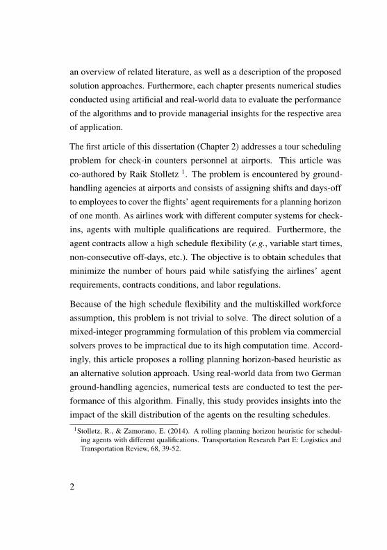
The first article of this dissertation (Chapter 2) addresses a tour schedulingproblem for check-in counters personnel at airports. This article wasco-authored by Raik Stolletz 1. The problem is encountered by ground-handling agencies at airports and consists of assigning shifts and days-offto employees to cover the flights’ agent requirements for a planning horizonof one month. As airlines work with different computer systems for check-ins, agents with multiple qualifications are required. Furthermore, theagent contracts allow a high schedule flexibility (e.g., variable start times,non-consecutive off-days, etc.). The objective is to obtain schedules thatminimize the number of hours paid while satisfying the airlines’ agentrequirements, contracts conditions, and labor regulations.

Because of the high schedule flexibility and the multiskilled workforceassumption, this problem is not trivial to solve. The direct solution of amixed-integer programming formulation of this problem via commercialsolvers proves to be impractical due to its high computation time. Accord-ingly, this article proposes a rolling planning horizon-based heuristic asan alternative solution approach. Using real-world data from two Germanground-handling agencies, numerical tests are conducted to test the per-formance of this algorithm. Finally, this study provides insights into theimpact of the skill distribution of the agents on the resulting schedules.

1Stolletz, R., & Zamorano, E. (2014). A rolling planning horizon heuristic for schedul-ing agents with different qualifications. Transportation Research Part E: Logistics andTransportation Review, 68, 39-52.

2

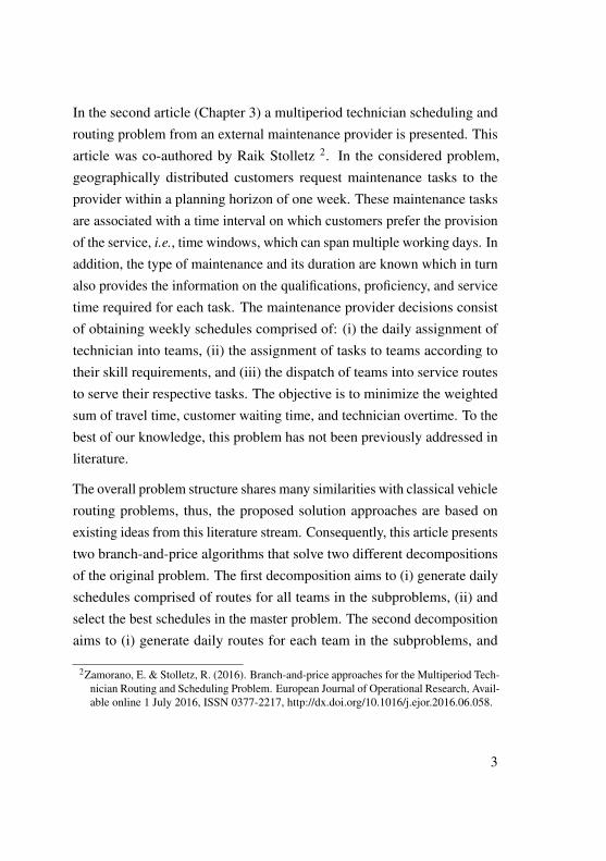
In the second article (Chapter 3) a multiperiod technician scheduling androuting problem from an external maintenance provider is presented. Thisarticle was co-authored by Raik Stolletz 2. In the considered problem,geographically distributed customers request maintenance tasks to theprovider within a planning horizon of one week. These maintenance tasksare associated with a time interval on which customers prefer the provisionof the service, i.e., time windows, which can span multiple working days. Inaddition, the type of maintenance and its duration are known which in turnalso provides the information on the qualifications, proficiency, and servicetime required for each task. The maintenance provider decisions consistof obtaining weekly schedules comprised of: (i) the daily assignment oftechnician into teams, (ii) the assignment of tasks to teams according totheir skill requirements, and (iii) the dispatch of teams into service routesto serve their respective tasks. The objective is to minimize the weightedsum of travel time, customer waiting time, and technician overtime. To thebest of our knowledge, this problem has not been previously addressed inliterature.

The overall problem structure shares many similarities with classical vehiclerouting problems, thus, the proposed solution approaches are based onexisting ideas from this literature stream. Consequently, this article presentstwo branch-and-price algorithms that solve two different decompositionsof the original problem. The first decomposition aims to (i) generate dailyschedules comprised of routes for all teams in the subproblems, (ii) andselect the best schedules in the master problem. The second decompositionaims to (i) generate daily routes for each team in the subproblems, and

2Zamorano, E. & Stolletz, R. (2016). Branch-and-price approaches for the Multiperiod Tech-nician Routing and Scheduling Problem. European Journal of Operational Research, Avail-able online 1 July 2016, ISSN 0377-2217, http://dx.doi.org/10.1016/j.ejor.2016.06.058.

3

(ii) select the best team-day routes in the master problem. The numericaltests in this article evaluate the performance of the proposed algorithmsand compare it to the performance of commercial solvers. Artificial databased on known benchmark data sets and real-world data from a forkliftmaintenance provider are used for this purpose. Accordingly, insightsinto the impact of time window length on computation time and objectivefunction value are given.

The third article (Chapter 4) presents a task scheduling problem for check-in personnel at airports. This article is a joined work with Annika Beckerand Raik Stolletz 3. Similar to Chapter 2, this problem is encounteredby ground-handling agencies at airports. Nonetheless, it belongs to anoperational planning stage which consists of determining a daily assignmentof multiskilled agents to flights (check-in and boarding) such that the agentrequirements defined by the airlines are fulfilled. As check-in counterscan be located in different gates at an airport, change-over times needto be considered in the assignment process. In contrast to classical taskassignment models, in the current problem the end time of each task isfixed, and the processing time depends on the arrival time of the agentto the counter. The objective is to minimize the weighted sum of agenttraveling time, overtime, tardiness, and outsourcing.

The solution approach proposed in this article resembles the one presentedin Chapter 3, as this task assignment problem also involves routing deci-sions. Accordingly, a branch-and-price algorithm that solves a decompo-sition of the task assignment problem is presented. In this case, however,the original problem is decomposed into (i) subproblems that generate

3Zamorano, E., Becker, A. & Stolletz, R. (2016). Task assignment with start time-dependentprocessing times for personnel at check-in counters. Working paper, under considerationfor publication.

4

flight assignments per agent, and (ii) a master problem that selects the bestassignments. In a numerical study, real-world data from a German ground-handling agency are used to compare the performance of the proposedalgorithm to the performance of the direct solution via commercial solvers.Additional tests are conducted to provide insights into the impact of thetardiness limit on the overall schedules.

5

2. A Rolling Planning Horizon Heuristic forScheduling Agents with DifferentQualifications

Co-authors:

Raik StolletzChair of Production Management, Business School, University ofMannheim, Germany

Published in:

Transportation Research Part E: (TRE),Volume 68 (2014), pages 39-52, DOI: 10.1016/j.tre.2014.05.002

Abstract:

At airports, the workforce for check-in services is managed by ground-handling companies. Although the time-dependent agent requirements areknown, the scheduling process is complex because agents operate differentcheck-in systems and contracts allow scheduling flexibility. We proposea Mixed Integer Programming model based on the Reduced Set-Coveringformulation for the monthly tour scheduling problem for a workforce withmultiple non-hierarchical qualifications. We present a rolling planning

7

horizon-based heuristic to solve this problem. Our heuristic provides near-optimal schedules within reasonable computation time for real-world cases.In addition, we provide insights into the impact of the skill distribution onthe scheduling costs.

2.1. Introduction

Third-party ground-handling agencies provide passenger handling services,such as check-in of passengers at airport terminals, to airlines. After therelease in 1996 of Directive 96/67/EC on the liberalization of the ground-handling market at European airports, the number of third-party groundhandlers increased by 90% in five years (SH&E, 2002), leading to highercompetition and price reductions (Airport Research Center, 2009). Becausestaff costs represent 66% to 75% of ground handlers’ operating costs,optimized workforce schedules significantly increase their profitability(Steer Davies Gleave, 2010).

A typical workforce planning process undergone by ground-handling agen-cies is divided into four sub-stages, each with different planning horizons,objectives, and constraints: (i) head count planning, (ii) tour scheduling,(iii) task assignment, and (iv) replanning (Stolletz, 2010). Our work focuseson the second phase of this process: monthly tour scheduling. This decisionproblem consists of assigning individual employees to tours (e.g., dailyshifts and days off) to satisfy the time-dependent employee requirementsfor check-in of individual flights. The requirements are driven by the flightschedule and depend on the contract with the airline. Airlines work withdifferent computer systems for their check-in processes, and only qualifiedagents are allowed to operate them. Agents can be cross-trained, and it ispossible for them to switch between different systems during a working

8

shift. Agent assignment also must satisfy rules based on the contractsand qualifications of the employees. The objective of this planning taskis to minimize operative workforce costs with respect to the given pool ofagents and their individual contracts while ensuring that enough qualifiedemployees are assigned to cover the demand over the course of each day.

This paper presents a Mixed Integer Programming (MIP) model for tourscheduling with multiple skills. The consideration of multiple skills pre-vents a solution for the MIP in short CPU times with standard software.Therefore, this study presents a new heuristic based on a rolling planninghorizon approach. The main idea is to decompose the main tour schedulingproblem for multiple weeks into smaller but well-connected subproblemsthat cover only part of the entire planning horizon. To the best of our knowl-edge, no previous efforts have been directed toward applying a rollingplanning horizon to the problem at hand.

This paper is organized as follows: Section 2.2 gives an overview of relatedwork. Section 2.3 presents a description of the problem and the formulationas an MIP. The Rolling Planning Horizon heuristic (RPH) is described inSection 2.4. The numerical studies described in Section 2.5 demonstrate thereliability of the solution of the RPH compared to that of the MIP, obtainedfor data from different ground-handling agencies. A sensitivity analysisshows the impact of the skill distribution on the overall scheduling costs.Concluding remarks and managerial insights are presented in Section 2.6.

2.2. Previous research

Reviews of decision models and solution approaches in workforce schedul-ing and in particular tour scheduling are given in Alfares (2004), Ernst et al.

9

(2004b), Ernst et al. (2004a), and Van den Bergh et al. (2013). Models fortour scheduling with multiple qualified agents often assume hierarchicalskill sets; see, for example, Rong and Grunow (2009). In this case, employ-ees with higher skill levels are allowed to be assigned to jobs that requirelower skill levels. The general non-hierarchical model can solve this as aspecial case.

Eitzen et al. (2004) provide a generalized set-covering formulation for thefortnightly scheduling of multiskilled full- and part-time employees. Theypropose three different solution techniques (column expansion, columnsubset, and branch and price) and conduct numerical tests for probleminstances with different numbers of skill levels, workforce sizes and demandpatterns. Compared to our model, their shift and tour building rules are lessflexible (i.e., a smaller number of tour combinations are possible), and skillswitching during a shift is forbidden.

Love Jr. and Hoey (1990), Loucks and Jacobs (1991), and Hojati and Patil(2011) address tour scheduling problems in the fast food industry. Theyconsider a workforce with limited availability (i.e., agents are eligible towork only during specific time windows) and shifts and tours of variablelength. As with our application, agents are cross-trained and allowed tochange the tasks they are assigned to during a shift. Love Jr. and Hoey(1990)’s work differs from ours in that the surplus of working hours, skills,availability of employees and number of working days are modeled as co-efficients of the shifts to be assigned in the objective function. In addition,their solution technique differs from ours in that it consists of decomposingthe tour scheduling problem into two network flow subproblems: construc-tion of tours and allocation of tours to employees with the objective ofminimizing the surplus of manpower.

10

Loucks and Jacobs (1991), in contrast to our application, propose a multi-criteria optimization model to minimize the total man-hours of overstaffingand minimize the deviation from target working hours. Their solutionapproach mainly differs from ours in that shifts are determined by concate-nating segments (each segment corresponding to a different task), whilethe shift and tour building rules (minimum shift length, maximum shiftlength, maximum number of working days, etc.) are modeled implicitly asconstraints. Their approach also differs from ours in that they propose atwo-phase procedure: (i) a construction phase in which rules are used toassign task-segments to employees while relaxing the maximum number ofworking days constraint and (ii) an improvement phase in which violationsto this constraint are eliminated and other measures (overstaffing, deviationfrom target hours, etc.) are improved.

Hojati and Patil (2011) revisit the model proposed by Loucks and Jacobs(1991) and propose another solution approach. Their approach differsfrom ours in that they decompose the main problem into a two-phasealgorithm: (i) determining good shifts via a linear program that maximizesthe total number of eligible and available employees and (ii) assigningshifts to employees through the use of an integer linear programming-basedheuristic that determines all the shifts to be assigned to an employee, oneemployee at a time.

To address the complexity of tour scheduling problems, the aforementionedpapers propose different decomposition approaches. As Bartholdi (1981)shows, standard tour scheduling problems are already NP-complete. Withthe combination of flexible schedules and multiple non-hierarchical skills,additional complexity is expected. The basis of our heuristic is the rollingplanning horizon approach, an idea commonly used in production schedul-

11

ing to provide partial production schedules (e.g., on a weekly basis) forlonger planning periods; see Modigliani (1955), Baker (1977) and Bakerand Peterson (1979). This approach can also be used to decrease the sizeof a planning problem by solving a series of multi-period subproblems that,in the end, cover the entire planning horizon of the original problem.

Aside from production scheduling, few efforts have been directed at apply-ing a rolling planning horizon approach to workforce scheduling. Examplesof general workforce scheduling problems using a rolling horizon approachare the allocation of flexible employees to workstations in a productionline (Gronalt, 2003) and reactive nurse scheduling (Bard and Purnomo,2005). In the tour scheduling literature we find that Day and Ryan (1997)address a fortnightly tour scheduling problem for flight attendants for short-haul flights. In their solution method, they divide the main problem into adays-off allocation and lines of work construction subproblems. For thelatter, they apply a two-phase procedure by which they (i) construct linesof work based on a days-off template and (ii) improve the lines of workusing a branch-and-price algorithm. They make use of a rolling horizonbased-procedure to link these two steps recursively. Nevertheless, to thebest of our knowledge, no previous efforts have been directed toward thedevelopment of a rolling horizon-based procedure for the tour schedulingproblem as a whole.

2.3. Problem Description and Model Formulation

This study considers the tour scheduling problem for check-in counters withdiscontinuous schedules, i.e., with no overlap between shifts on differentdays. The planning horizon spans D days (d = 1, ...,D), and each day isdivided into T periods (t = 1, ...,T ) of equal length. Based on the flight

12

schedules and the contracts between the ground handler and the airlines,the agent requirements are known. These requirements r

qdt

specify thenumber of employees with a specific skill q needed in check-in counters onday d in period t . The goal is to assign each employee e to a shift of typej on day d such that the agent requirements are covered and the overallscheduling costs are minimized.

With respect to multiple qualifications, each employee e can be differentlyqualified and cross-trained. The set of skills of each employee is reflectedin the parameter g

eq

, with a value of 1 if employee e has skill q and 0

otherwise.

The working conditions regarding schedules are established by the ground-handling agency in the employee contracts. The following regulations areconsidered:

• Shifts can vary in length between 3 and 10 hours.

• Shifts can start at any period t on day d and at different times ondifferent days.

• A minimum resting time of R hours between shifts needs to berespected.

• A maximum of w consecutive workdays without a day off is allowed.Days off can be non-consecutive.

• There is no limit on the total working hours per week. The overallnumber of workdays must remain grater than d

min

e

and less thand

max

e

days during the planning horizon of D days.

• At most hmax

e

working hours per month are allowed per employee.

13

The operational costs consist of two elements:

• Paid hours, i.e., total working hours.

• Overtime costs, i.e., if hmax

e

is exceeded, the respective overtimeperiods ot

e

have an additional cost of cot per period.

A commonly used formulation for tour scheduling problems is the set-covering formulation proposed by Dantzig (1954); see also Ernst et al.(2004b). This MIP formulation uses a matrix with all possible combina-tions of tours (daily shifts and days off) as input that are to be assignedto employees to meet the requirements per period. However, in our case,the flexibility of the schedules and the heterogeneity of the workforce pro-duces a tour matrix with a large amount of data, thus making the solutionintractable. Stolletz (2010) proposes a Reduced Set-Covering (RSC) for-mulation for the tour scheduling problem with single skills. This approachrequires a matrix of all possible daily shifts only. The tour-building rules(maximum and minimum overall working days, maximum consecutiveworking days, etc.) are then modeled implicitly. This study extends theRSC formulation to a Multiskilled Workforce Scheduling (MWS) model.Table 2.1 summarizes the notation used.

Four main decision variables are used. First, the binary variable p

ejd

assigns employees to shifts on a day.

p

ejd

=

8<

:1, if employee e is assigned to shift j on day d and

0, otherwise.(2.1)

Second, the skill that an employee applies to work in each period t on dayd is selected through binary variable z

eqtd

:

14

z

eqtd

=

8<

:1, if employee e uses skill q in period t of day d and

0, otherwise.(2.2)

Third, we use an auxiliary variable y

ed

to indicate whether an employeeworks on a particular day:

y

ed

=

8<

:1, if employee e is assigned to work on day d and

0, otherwise.(2.3)

Last, the number of exceeding periods over the monthly hour limit hmax

e

per employee are determined by the variable ot

e

.

In case the requirements are not met in a particular period within a day,outsourcing additional resources is allowed and decided upon using integervariable o

qtd

. This ensures feasibility independent of the problem instance.This variable is also paired with an outsourcing cost cout

q

, which could beinterpreted as the penalty for unmet requirements.

The staffing costs c

ej

for a certain shift j depend on the length of shiftj and the number of skills employee e has (see Equation (2.4)). Thenumber of working periods is obtained from the difference between thelast working period (f

j

) and the first working period (sj

) of shift j . In casethe hourly wage per period depends on an agent’s number of qualifications,the cost depends on the number of qualifications per agent multiplied by adifferentiation factor ↵:

15

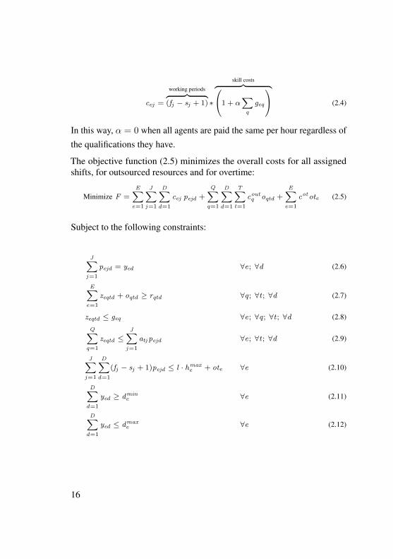
c

ej

=

working periodsz }| {(f

j

� s

j

+ 1) ⇤

skill costsz }| {0

@1 + ↵

X

q

g

eq

1

A (2.4)

In this way, ↵ = 0 when all agents are paid the same per hour regardless ofthe qualifications they have.

The objective function (2.5) minimizes the overall costs for all assignedshifts, for outsourced resources and for overtime:

Minimize F =

EX

e=1

JX

j=1

DX

d=1

c

ej

p

ejd

+

QX

q=1

DX

d=1

TX

t=1

c

out

q

o

qtd

+

EX

e=1

c

ot

ot

e

(2.5)

Subject to the following constraints:

JX

j=1

p

ejd

= y

ed

8e; 8d (2.6)

EX

e=1

z

eqtd

+ o

qtd

� r

qtd

8q; 8t ; 8d (2.7)

z

eqtd

g

eq

8e; 8q; 8t ; 8d (2.8)QX

q=1

z

eqtd

JX

j=1

a

tj

p

ejd

8e; 8t ; 8d (2.9)

JX

j=1

DX

d=1

(f

j

� s

j

+ 1)p

ejd

l · hmax

e

+ ot

e

8e (2.10)

DX

d=1

y

ed

� d

min

e

8e (2.11)

DX

d=1

y

ed

d

max

e

8e (2.12)

16

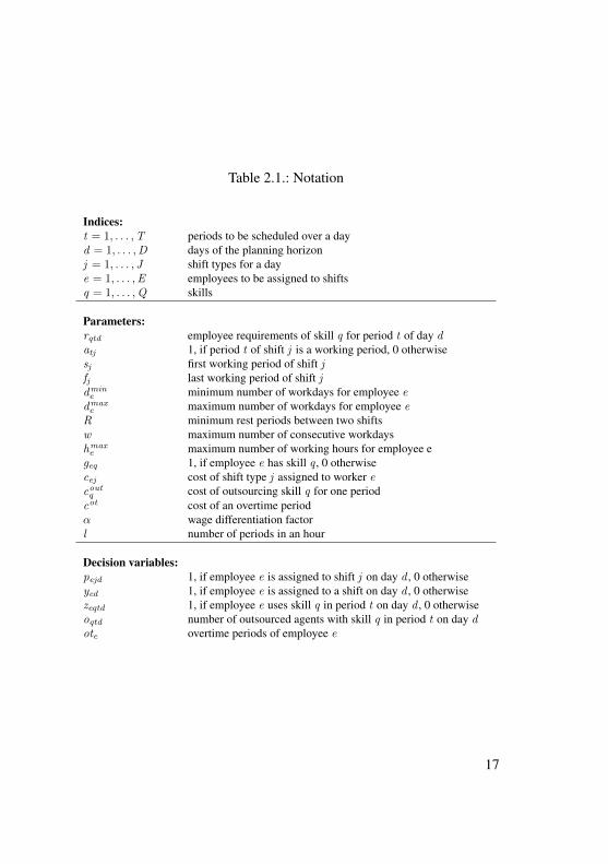
Table 2.1.: Notation

Indices:t = 1, . . . ,T periods to be scheduled over a dayd = 1, . . . ,D days of the planning horizonj = 1, . . . , J shift types for a daye = 1, . . . ,E employees to be assigned to shiftsq = 1, . . . ,Q skills

Parameters:r

qtd

employee requirements of skill q for period t of day d

a

tj

1, if period t of shift j is a working period, 0 otherwises

j

first working period of shift jf

j

last working period of shift jd

min

e

minimum number of workdays for employee e

d

max

e

maximum number of workdays for employee e

R minimum rest periods between two shiftsw maximum number of consecutive workdaysh

max

e

maximum number of working hours for employee eg

eq

1, if employee e has skill q , 0 otherwisec

ej

cost of shift type j assigned to worker ec

out

q

cost of outsourcing skill q for one periodc

ot cost of an overtime period↵ wage differentiation factorl number of periods in an hour

Decision variables:p

ejd

1, if employee e is assigned to shift j on day d , 0 otherwisey

ed

1, if employee e is assigned to a shift on day d , 0 otherwisez

eqtd

1, if employee e uses skill q in period t on day d , 0 otherwiseo

qtd

number of outsourced agents with skill q in period t on day d

ot

e

overtime periods of employee e

17

d+wX

d=d

y

ed

w 8e; 8d D � w (2.13)

T �JX

j=1

f

j

p

ejd

+

JX

j=1

s

j

p

ejd+1 � y

ed+1 � y

ed+1 R 8e; 8d D � 1 (2.14)

p

ejd

; y

ed

; z

eqtd

2 {0, 1} 8e; 8j ; 8q; 8t ; 8d (2.15)

ot

e

� 0 8e (2.16)

Constraints (2.6) and (2.11) to (2.15) are equivalent to those in the formu-lation proposed by Stolletz (2010), while the objective function (2.5) andconstraints (2.7) to (2.10) and (2.16) extend the formulation to a multi-skilled workforce. Constraint (2.6) ensures that employee e is assigned toat most one shift per day and sets the variable y

ed

. Equation (2.7) ensuresthat agent requirements are satisfied for each skill q , either by assigningagents or by outsourcing. Equation (2.8) ensures that employees are as-signed to tasks for which they are qualified. An agent can be assigned toat most one task if the respective period is a working period, as stated inEquation (2.9). Equation (2.10) ensures that employees are assigned toat most hmax

e

overall working hours, otherwise incurring an overtime ofot

e

periods. Constraints (2.11) and (2.12) represent the lower and upperbounds for the overall working days within a tour, while Equation (2.13)allows employees to work a maximum of w consecutive days. Equation(2.14) ensures that the sum of the off periods after the end of a shift on dayd plus those before starting a shift on day d + 1 is at least R periods long.

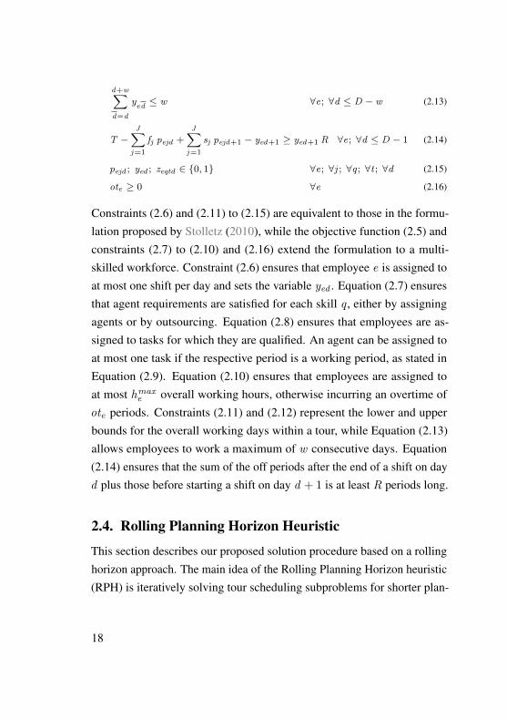
2.4. Rolling Planning Horizon HeuristicThis section describes our proposed solution procedure based on a rollinghorizon approach. The main idea of the Rolling Planning Horizon heuristic(RPH) is iteratively solving tour scheduling subproblems for shorter plan-

18

ning horizons and freezing the variables for the first days in each iteration(see Fig. 2.1). In iteration k = 1, the RPH starts with solving the subprob-lem for the first r days of the planning horizon. The decision variables forthe first s r days are fixed to their solution values. The next iterationk = 2 solves the problem up to day s + r , with the decision variablesfixed up to day s . While this subproblem is being solved, the tour-buildingconstraints respect the already fixed schedule. For a certain iteration k , thesubproblem is based on an already fixed schedule for (k � 1)s days andcovers (k � 1)s + r days. After solving the MIP, the decision variablesfor day (k � 1)s + 1 up to day ks are also fixed. In the last iteration, itis ensured that the remainder of the original planning horizon is covered,especially when D is not a multiple of s .

Figure 2.1.: RPH example

To avoid infeasibility, the bounds on the overall working days and overallworking hours have to be changed. Specifically, the bounds set in con-straints (2.10), (2.11), and (2.12) need to be replaced, because they consider

19

the full length of the planning horizon. The idea is to set different bounds

in each iteration k < K that are related to the proportion(k � 1)s + r

D

ofthe considered planning horizon:

JX

j=1

(k�1)s+rX

d=1

(f

j

� s

j

+ 1)p

ejd

⇠[(k � 1)s + r ] · l · hmax

e

D

⇡+ ot

e

8e (2.17)

(k�1)s+rX

d=1

y

ed

��[(k � 1)s + r ]d

min

e

D

⌫8e, (2.18)

(k�1)s+rX

d=1

y

ed

⇠[(k � 1)s + r ]d

max

e

D

⇡8e, (2.19)

Constraints (2.17)-(2.19) bind the sum of the overall assigned workinghours and days up to (k � 1)s + r to the ratio of the minimum and max-imum hours and days, respectively. In this way, the bounds are updatedin every iteration. Nevertheless, these new constraints still constitute hardconstraints that strictly bind the length of each tour to a fraction of theworking-days limit defined in the problem setting. The last iteration K runswith the original bounds and applies the constraints (2.17)-(2.19) in placeof (2.10)-(2.12), which cover the entire planning horizon. Algorithm 1shows the pseudocode for the RPH procedure.

20

Algorithm 1 RPH Pseudocode

for k = 1 to⇠D

s

⇡� 1 do

Solve MWS subject to (2.6)-(2.9), (2.13)-(2.16) and (2.17)-(2.19) ford (k � 1)s + r with fixed decision variables up to d = (k � 1)s

for d = (k � 1)s + 1 to ks doFix y

ed

, oqdt

, zeqtd

and p

ejd

end forend forSolve MWS subject to (2.6)-(2.16) for d D with fixed decisionvariables up to d = (K � 1)s

2.5. Numerical Experiments

For our numerical tests, we analyze cases of two German ground-handlingagencies. In the first case, we use the demand data from one ground handlerto obtain good parameters r and s for the RPH. To focus on this goal, weassume fully qualified agents in Section 2.5.1. In Section 2.5.2, the samedemand data are used to analyze the impact of different skill distributionson the quality of the schedules. In the second case, we test our proposedheuristic with data from a second ground-handling agency, which containmore information regarding the workforce configuration (Section 2.5.3).The MWS model and the subproblems of the RPH heuristic were solvedusing the Gurobi 4.6.1 solver on a 2.5-GHz Intel Core i7 machine with 8GB of RAM.

21

2.5.1. Sensitivity of the RPH Parameters

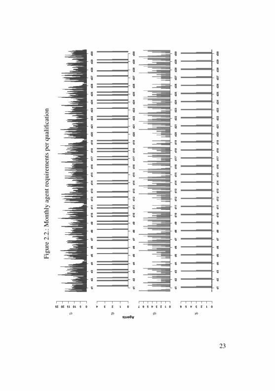
For the first numerical tests, we study the impact of the choice of theparameters r and s on the performance of the RPH. The data from the firstground-handling agency contain the aggregated agent skill requirementsfor 30-minute intervals during the opening hours (T = 34) for differentqualifications (Q = 4) within a 30-day planning horizon (D = 30) (seeFig. 2.2). The workforce consists of E = 65 employees. Because no realinformation on the skill distribution was given, we consider agents with allskills (i.e., generalists) and no wage differentiation (↵ = 0). The employeecontracts establish a maximum of w = 6 consecutive working days withouta day off and a minimum of dmin

e

= 19 and maximum of dmax

e

= 23

overall working days per employee. Shifts can be from 3 to 10 hours inlength, with a minimum of R = 10 resting hours between consecutiveworking days. We assume there are no limits on the maximum overallworking hours hmax

e

. The costs consist of scheduled hours and outsourcedhours (with cout

q

= 1⇥10

7), and no overtime costs (cot

= 0) are considered.We test different values of the RPH’s parameters r = 3, 4, 5, ..., 15 ands = 2, 3, 4.

Solving the MWS MIP model with this setting to optimality yields a totalof 7,941.5 scheduled hours with an overcapacity of 543.5 hours and nooutsourcing. This optimal solution was found in 16,742 seconds. Table2.2 shows the overall scheduled hours, outsourced hours, the overcapacity(in hours), and the computation time (in seconds) obtained for each testinstance of the RPH. The absolute gap to the optimal scheduled hours ofthe RPH, compared to the optimal solution, is shown in the last column.The absolute gap is only reported for instances without outsourcing (50%

22

Figu

re2.

2.:M

onth

lyag

entr

equi

rem

ents

perq

ualifi

catio

n

q1

0510152025

d1d2

d3d4

d5d6

d7d8

d9d10

d11

d12

d13

d14

d15

d16

d17

d18

d19

d20

d21

d22

d23

d24

d25

d26

d27

d28

d29

d30

q2

01234

d1d2

d3d4

d5d6

d7d8

d9d10

d11

d12

d13

d14

d15

d16

d17

d18

d19

d20

d21

d22

d23

d24

d25

d26

d27

d28

d29

d30

q3

01234567

d1d2

d3d4

d5d6

d7d8

d9d10

d11

d12

d13

d14

d15

d16

d17

d18

d19

d20

d21

d22

d23

d24

d25

d26

d27

d28

d29

d30

q4

0123456

d1d2

d3d4

d5d6

d7d8

d9d10

d11

d12

d13

d14

d15

d16

d17

d18

d19

d20

d21

d22

d23

d24

d25

d26

d27

d28

d29

d30

Agents

23

of the cases) because the optimal solution does not include any outsourcedperiods. For the instance considered, there is no combination of r and s

that clearly outperforms the others. Nevertheless, the configuration r = 7

and s = 4 had the lowest computation times and an acceptable optimalitygap among the cases with no outsourcing.

To show that this configuration results in good solutions for other probleminstances, we scale the workforce and the requirements. For this purpose,we multiply the demand and the workforce size by a scaling factor � tosimulate scenarios with lower demand and a smaller workforce (� < 1)or higher demand and a larger workforce (� > 1) than the original setting.We solve the RPH with r = 7 and s = 4 for several values of the scalingfactor � = 0.2, 0.4, ..., 1.4 and compare the solutions to the those from theMIP formulation. Table 2.3 shows, for each �, the workforce size, theoverall requirements (in hours), the overall scheduled hours, the sum ofthe outsourced hours, the overcapacity (in hours) and the computation time(in seconds). The last column shows the ratio of outsourced hours (as apercentage of the required hours) for each problem instance. Although formost of the instances, outsourcing is required according to the RPH results,the ratio of outsourced hours does not exceed 1.15%. The computation timeof the RPH is considerably lower than that of the exact solution in all cases.In the case of � = 0.2 an exact solution could not be found even after 33hours of computation. This confirms that the configuration selected can beapplied to different problem sizes, although testing different configurationsof the RPH parameters for different problem instances is recommended.

24

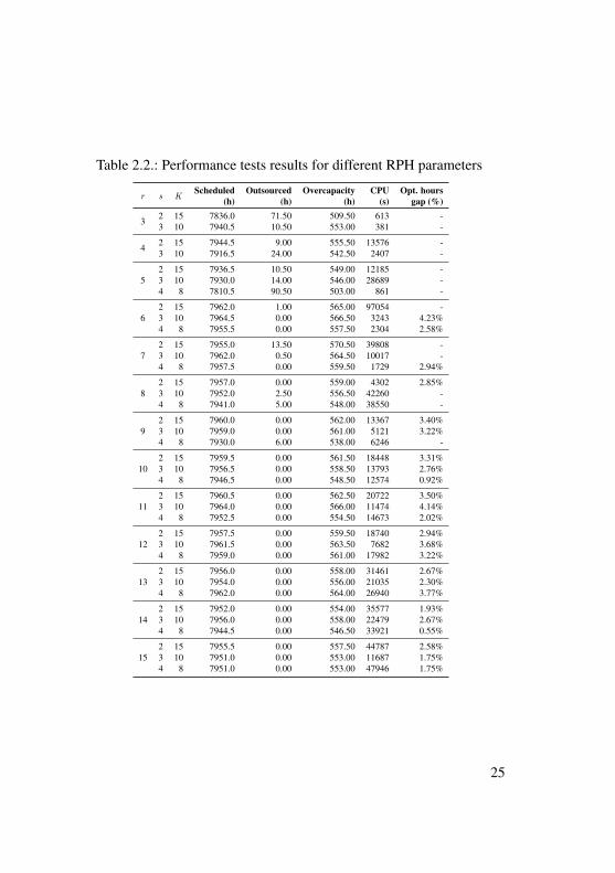
Table 2.2.: Performance tests results for different RPH parameters

r s K

Scheduled Outsourced Overcapacity CPU Opt. hours(h) (h) (h) (s) gap (%)

3 2 15 7836.0 71.50 509.50 613 -3 10 7940.5 10.50 553.00 381 -

4 2 15 7944.5 9.00 555.50 13576 -3 10 7916.5 24.00 542.50 2407 -

52 15 7936.5 10.50 549.00 12185 -3 10 7930.0 14.00 546.00 28689 -4 8 7810.5 90.50 503.00 861 -

62 15 7962.0 1.00 565.00 97054 -3 10 7964.5 0.00 566.50 3243 4.23%4 8 7955.5 0.00 557.50 2304 2.58%

72 15 7955.0 13.50 570.50 39808 -3 10 7962.0 0.50 564.50 10017 -4 8 7957.5 0.00 559.50 1729 2.94%

82 15 7957.0 0.00 559.00 4302 2.85%3 10 7952.0 2.50 556.50 42260 -4 8 7941.0 5.00 548.00 38550 -

92 15 7960.0 0.00 562.00 13367 3.40%3 10 7959.0 0.00 561.00 5121 3.22%4 8 7930.0 6.00 538.00 6246 -

102 15 7959.5 0.00 561.50 18448 3.31%3 10 7956.5 0.00 558.50 13793 2.76%4 8 7946.5 0.00 548.50 12574 0.92%

112 15 7960.5 0.00 562.50 20722 3.50%3 10 7964.0 0.00 566.00 11474 4.14%4 8 7952.5 0.00 554.50 14673 2.02%

122 15 7957.5 0.00 559.50 18740 2.94%3 10 7961.5 0.00 563.50 7682 3.68%4 8 7959.0 0.00 561.00 17982 3.22%

132 15 7956.0 0.00 558.00 31461 2.67%3 10 7954.0 0.00 556.00 21035 2.30%4 8 7962.0 0.00 564.00 26940 3.77%

142 15 7952.0 0.00 554.00 35577 1.93%3 10 7956.0 0.00 558.00 22479 2.67%4 8 7944.5 0.00 546.50 33921 0.55%

152 15 7955.5 0.00 557.50 44787 2.58%3 10 7951.0 0.00 553.00 11687 1.75%4 8 7951.0 0.00 553.00 47946 1.75%

25

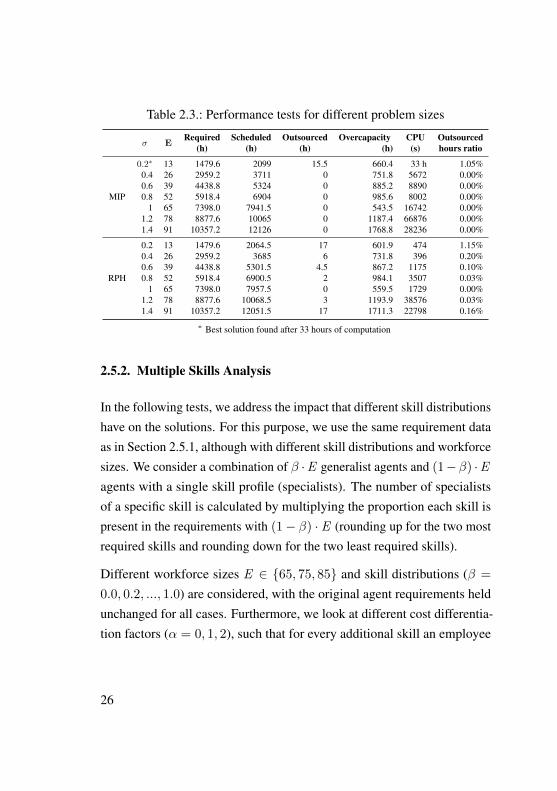
Table 2.3.: Performance tests for different problem sizes

� ERequired Scheduled Outsourced Overcapacity CPU Outsourced

(h) (h) (h) (h) (s) hours ratio

MIP

0.2⇤ 13 1479.6 2099 15.5 660.4 33 h 1.05%0.4 26 2959.2 3711 0 751.8 5672 0.00%0.6 39 4438.8 5324 0 885.2 8890 0.00%0.8 52 5918.4 6904 0 985.6 8002 0.00%

1 65 7398.0 7941.5 0 543.5 16742 0.00%1.2 78 8877.6 10065 0 1187.4 66876 0.00%1.4 91 10357.2 12126 0 1768.8 28236 0.00%

RPH

0.2 13 1479.6 2064.5 17 601.9 474 1.15%0.4 26 2959.2 3685 6 731.8 396 0.20%0.6 39 4438.8 5301.5 4.5 867.2 1175 0.10%0.8 52 5918.4 6900.5 2 984.1 3507 0.03%

1 65 7398.0 7957.5 0 559.5 1729 0.00%1.2 78 8877.6 10068.5 3 1193.9 38576 0.03%1.4 91 10357.2 12051.5 17 1711.3 22798 0.16%

⇤ Best solution found after 33 hours of computation

2.5.2. Multiple Skills Analysis

In the following tests, we address the impact that different skill distributionshave on the solutions. For this purpose, we use the same requirement dataas in Section 2.5.1, although with different skill distributions and workforcesizes. We consider a combination of � ·E generalist agents and (1��) ·Eagents with a single skill profile (specialists). The number of specialistsof a specific skill is calculated by multiplying the proportion each skill ispresent in the requirements with (1� �) · E (rounding up for the two mostrequired skills and rounding down for the two least required skills).

Different workforce sizes E 2 {65, 75, 85} and skill distributions (� =

0.0, 0.2, ..., 1.0) are considered, with the original agent requirements heldunchanged for all cases. Furthermore, we look at different cost differentia-tion factors (↵ = 0, 1, 2), such that for every additional skill an employee

26

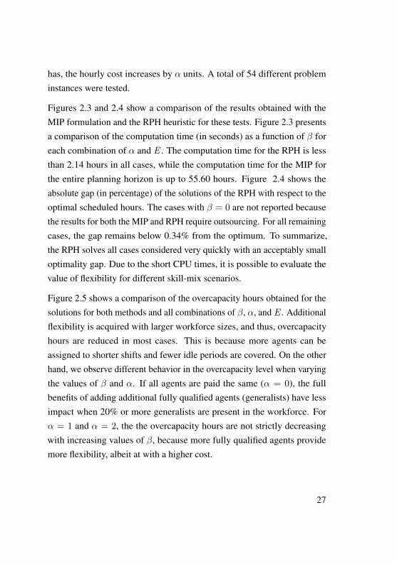
has, the hourly cost increases by ↵ units. A total of 54 different probleminstances were tested.

Figures 2.3 and 2.4 show a comparison of the results obtained with theMIP formulation and the RPH heuristic for these tests. Figure 2.3 presentsa comparison of the computation time (in seconds) as a function of � foreach combination of ↵ and E . The computation time for the RPH is lessthan 2.14 hours in all cases, while the computation time for the MIP forthe entire planning horizon is up to 55.60 hours. Figure 2.4 shows theabsolute gap (in percentage) of the solutions of the RPH with respect to theoptimal scheduled hours. The cases with � = 0 are not reported becausethe results for both the MIP and RPH require outsourcing. For all remainingcases, the gap remains below 0.34% from the optimum. To summarize,the RPH solves all cases considered very quickly with an acceptably smalloptimality gap. Due to the short CPU times, it is possible to evaluate thevalue of flexibility for different skill-mix scenarios.

Figure 2.5 shows a comparison of the overcapacity hours obtained for thesolutions for both methods and all combinations of �, ↵, and E . Additionalflexibility is acquired with larger workforce sizes, and thus, overcapacityhours are reduced in most cases. This is because more agents can beassigned to shorter shifts and fewer idle periods are covered. On the otherhand, we observe different behavior in the overcapacity level when varyingthe values of � and ↵. If all agents are paid the same (↵ = 0), the fullbenefits of adding additional fully qualified agents (generalists) have lessimpact when 20% or more generalists are present in the workforce. For↵ = 1 and ↵ = 2, the the overcapacity hours are not strictly decreasingwith increasing values of �, because more fully qualified agents providemore flexibility, albeit at with a higher cost.

27

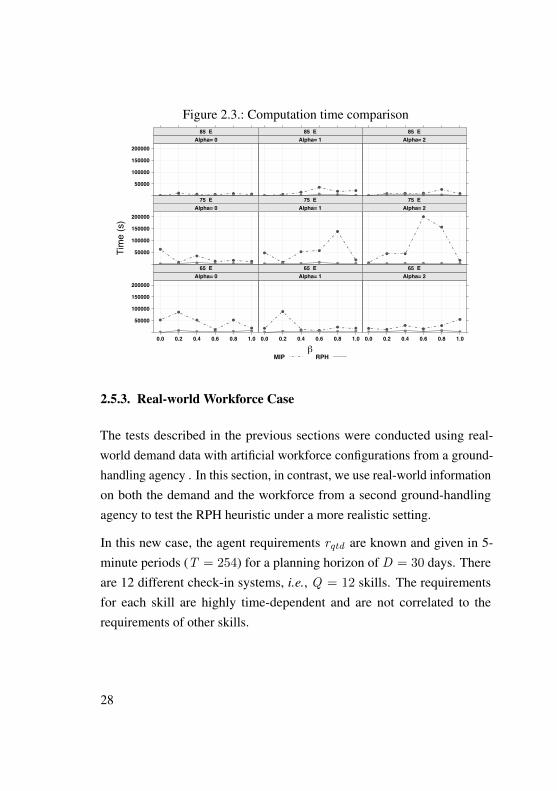
Figure 2.3.: Computation time comparison

β

Tim

e (s

)

50000

100000

150000

200000

0.0 0.2 0.4 0.6 0.8 1.0

●

●

●

●

●

●

●● ● ● ● ●

Alpha= 065 E

0.0 0.2 0.4 0.6 0.8 1.0

●

●

● ●

● ●

● ● ● ● ● ●

Alpha= 165 E

0.0 0.2 0.4 0.6 0.8 1.0

● ●

●

●

●

●

● ● ● ● ● ●

Alpha= 265 E

50000

100000

150000

200000

●

●

●

● ● ●● ● ● ● ● ●

Alpha= 075 E

●

●

● ●

●

●

● ● ● ● ● ●

Alpha= 175 E

●

● ●

●

●

●

● ● ● ● ● ●

Alpha= 275 E

50000

100000

150000

200000

●● ● ● ● ●

● ● ● ● ● ●

Alpha= 085 E

● ●●

●

● ●

● ● ● ● ● ●

Alpha= 185 E

●● ● ●

●

●● ● ● ● ● ●

Alpha= 285 E

MIP RPH

2.5.3. Real-world Workforce Case

The tests described in the previous sections were conducted using real-world demand data with artificial workforce configurations from a ground-handling agency . In this section, in contrast, we use real-world informationon both the demand and the workforce from a second ground-handlingagency to test the RPH heuristic under a more realistic setting.

In this new case, the agent requirements r

qtd

are known and given in 5-minute periods (T = 254) for a planning horizon of D = 30 days. Thereare 12 different check-in systems, i.e., Q = 12 skills. The requirementsfor each skill are highly time-dependent and are not correlated to therequirements of other skills.

28

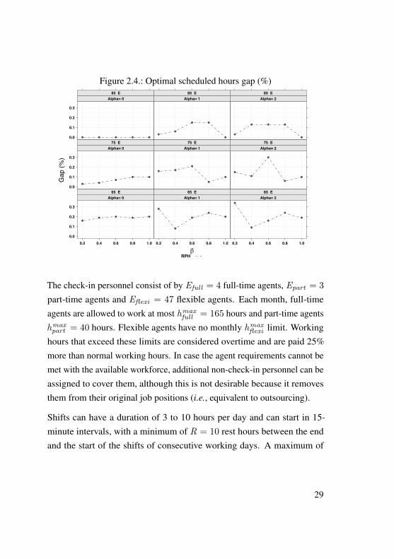
Figure 2.4.: Optimal scheduled hours gap (%)

β

Gap

(%)

0.0

0.1

0.2

0.3

0.2 0.4 0.6 0.8 1.0

●

●●

●●

Alpha= 065 E

0.2 0.4 0.6 0.8 1.0

●

●

●

●

●

Alpha= 165 E

0.2 0.4 0.6 0.8 1.0

●

●

●

●

●

Alpha= 265 E

0.0

0.1

0.2

0.3

●●

●

● ●

Alpha= 075 E

●●

●

●

●

Alpha= 175 E

●

●

●

●

●

Alpha= 275 E

0.0

0.1

0.2

0.3

● ● ● ● ●

Alpha= 085 E

●

●

● ●

●

Alpha= 185 E

●

● ● ●

●

Alpha= 285 E

RPH

The check-in personnel consist of by E

full

= 4 full-time agents, Epart

= 3

part-time agents and E

flexi

= 47 flexible agents. Each month, full-timeagents are allowed to work at most hmax

full

= 165 hours and part-time agentsh

max

part

= 40 hours. Flexible agents have no monthly h

max

flexi

limit. Workinghours that exceed these limits are considered overtime and are paid 25%more than normal working hours. In case the agent requirements cannot bemet with the available workforce, additional non-check-in personnel can beassigned to cover them, although this is not desirable because it removesthem from their original job positions (i.e., equivalent to outsourcing).

Shifts can have a duration of 3 to 10 hours per day and can start in 15-minute intervals, with a minimum of R = 10 rest hours between the endand the start of the shifts of consecutive working days. A maximum of

29

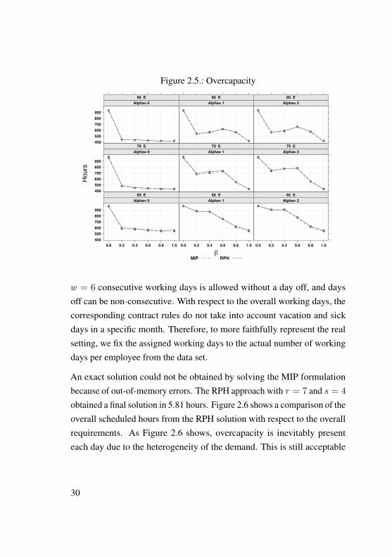
Figure 2.5.: OvercapacityOvercapacity

β

Hours

400500600700800900

0.0 0.2 0.4 0.6 0.8 1.0

●

● ●● ● ●

●

● ●● ● ●

Alpha= 065 E

0.0 0.2 0.4 0.6 0.8 1.0

●

● ●

●

●

●

●

● ●

●

●

●

Alpha= 165 E

0.0 0.2 0.4 0.6 0.8 1.0

●

● ●

●

●

●

●

● ●

●

●

●

Alpha= 265 E

400500600700800900

●

●● ● ● ●

●

●● ● ● ●

Alpha= 075 E

●

●●

●

●

●

●

●●

●

●

●

Alpha= 175 E

●

●

● ●

●

●

●

●● ●

●

●

Alpha= 275 E

400500600700800900 ●

● ● ● ● ●

●

● ● ● ● ●

Alpha= 085 E

●

●●

●

●

●

●

●●

●

●

●

Alpha= 185 E

●

●●

●

●

●

●

●●

●

●

●

Alpha= 285 E

MIP RPH

w = 6 consecutive working days is allowed without a day off, and daysoff can be non-consecutive. With respect to the overall working days, thecorresponding contract rules do not take into account vacation and sickdays in a specific month. Therefore, to more faithfully represent the realsetting, we fix the assigned working days to the actual number of workingdays per employee from the data set.

An exact solution could not be obtained by solving the MIP formulationbecause of out-of-memory errors. The RPH approach with r = 7 and s = 4

obtained a final solution in 5.81 hours. Figure 2.6 shows a comparison of theoverall scheduled hours from the RPH solution with respect to the overallrequirements. As Figure 2.6 shows, overcapacity is inevitably presenteach day due to the heterogeneity of the demand. This is still acceptable

30

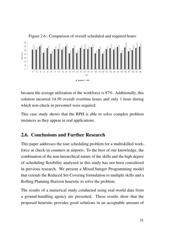
Figure 2.6.: Comparison of overall scheduled and required hours

Days

Agent−hours

020

4060

80100

120

140

d1 d2 d3 d4 d5 d6 d7 d8 d9 d10 d11 d12 d13 d14 d15 d16 d17 d18 d19 d20 d21 d22 d23 d24 d25 d26 d27 d28 d29 d30

Required RPH

because the average utilization of the workforce is 87%. Additionally, thissolution incurred 14.50 overall overtime hours and only 1 hour duringwhich non-check-in personnel were required.

This case study shows that the RPH is able to solve complex probleminstances as they appear in real applications.

2.6. Conclusions and Further Research

This paper addresses the tour scheduling problem for a multiskilled work-force at check-in counters at airports. To the best of our knowledge, thecombination of the non-hierarchical nature of the skills and the high degreeof scheduling flexibility analyzed in this study has not been consideredin previous research. We present a Mixed Integer Programming modelthat extends the Reduced Set-Covering formulation to multiple skills and aRolling Planning Horizon heuristic to solve the problem.

The results of a numerical study conducted using real-world data froma ground-handling agency are presented. These results show that theproposed heuristic provides good solutions in an acceptable amount of

31

time for different problem sizes and skill distributions. However, a properselection of the parameters for the RPH is crucial to the performance ofthe heuristic, and additional testing is recommended for different problemsettings. Furthermore, the results show that additional flexibility can begained by increasing the proportion of generalist agents in the workforce.On the other hand, this additional flexibility can be acquired at a highercost if salaries depend on the number of qualifications of the agents.

The results of additional tests conducted using data from a second ground-handling agency show that with our proposed heuristic, it is possible tosolve realistic problems that are otherwise not solvable with an MIP formu-lation, and to obtain good-quality solutions.

Further research needs to be conducted to extend the proposed model toconsider agent preferences and fairness measures in the planning process.Another research direction is to implement subsequent phases of the work-force planning process (e.g., task assignment and replanning) with thepresent model to serve as an integrative robust planning tool for ground-handling agencies.

32

3. Branch-and-price approaches for theMultiperiod Technician Routing andScheduling Problem

Co-author:

Raik StolletzChair of Production Management, Business School, University ofMannheim, Germany

Published in: European Journal of Operational Research,Available online 1 July 2016, ISSN 0377-2217, DOI:doi:10.1016/j.ejor.2016.06.058

Abstract:

This paper addresses a technician routing and scheduling problem motivatedby the case of an external maintenance provider. Technicians are proficientin different skills and paired into teams to perform maintenance tasks.Tasks are skill constrained and have time windows that may span multipledays. The objective is to determine the daily assignment of techniciansinto teams, of teams to tasks, and of teams to daily routes such that theoperation costs are minimized. We propose a mixed integer program and abranch-and-price algorithm to solve this problem. Exploiting the structure

33

of the problem, alternative formulations are used for the column generation-phase of the algorithm. Using real-world data from an external maintenanceprovider, we conduct numerical studies to evaluate the performance of ourproposed solution approaches.

3.1. Introduction

This paper addresses the Multiperiod Technician Routing and SchedulingProblem (MPTRSP) based on the case of an external maintenance provider(EMP) specialized in electric forklifts. Services offered by the consideredEMP include preventive and corrective maintenance, failure diagnoses, andthe delivery of spare parts and supplements to different geographicallydistributed customers. As these services are offered at the customers’locations, they require the visit of a team of technicians based on customers’service requests. Such requests may be either known in advance (e.g., inthe case of preventive maintenance based on yearly contracts and scheduledrepairs), or requested on demand (e.g., emergency repairs when breakdownsoccur). In this research we consider programmed maintenance tasks, i.e.,maintenance demand is deterministic and known in advance, because thecurrent problem constitutes one part of a hierarchical planning process forthe EMP.

These maintenance tasks have the following features:

• First, based on maintenance contracts, a time frame for the provisionof each task has been agreed upon with the respective customer. Inthis way, customers can specify the allowed time(s) (and day(s))on which a task can be performed, i.e., time windows are defined.These time windows can span several hours and possibly several

34

days depending on the type of service requested. For example, atask can be allowed between Monday at 9:00 am and Friday at 1:00pm, a corrective maintenance task between Tuesday at 4:00 pm andWednesday at 12:00 pm, or a delivery between Thursday at 9:00am and 4:00 pm. Due to the EMP’s working day duration limit,these time windows can be formulated as multiple alternative timewindows on consecutive days. Maintenance contracts incur a penaltyfee if a customer is visited after the latest starting time. The contractsalso define the maximum waiting time per customer.

• Second, a single customer can request more than one service; there-fore, multiple tasks might need to be performed at the same location.Due to safety requirements, however, tasks are not allowed to be leftunfinished or split, i.e., tasks are non-preemptive, and at most oneteam per task is allowed. Third, tasks’ service time and travel timeare known, as well as the minimum skill proficiency required foreach task.

As for the workforce, first, each day, technicians are paired into teamsand then dispatched to visit customers. Team compositions remain fixedfor the duration day (i.e., a technician is assigned to at most one teamper day), although different team compositions on different days is notforbidden. The number of teams and size of a team are defined based on thecompany’s safety policies, e.g. since some maintenance tasks for forkliftsrequire lifting heavy equipment. Each technician is qualified in certain skilldomains (e.g., hydraulics, mechanic, electric, etc.) and has a proficiencylevel in each domain (e.g., basic proficiency, medium proficiency, orexpert). Thus, team qualifications depend on the combined qualificationsof the team members. Second, on any given day, teams are dispatched

35

from the EMP’s location and need to return to it before closing time. If ateam returns after this time, overtime is incurred at a cost. Other workforcescheduling decisions, such as shift scheduling, days-off scheduling, andmeal-breaks placement are outside of the scope of this paper.

The planning problem faced by this EMP consists of obtaining weeklyschedules comprised by: (i) daily pairing of technicians into teams, (ii)assignment of teams to tasks, and (iii) dispatching teams into routes toperform their respective tasks. The goal is to obtain weekly schedules suchthat the operational costs are minimized. That is, the said schedules shouldminimize travel costs, customer waiting time and technician overtime. Tothe best of our knowledge, this problem with all its features has not beenpreviously addressed in literature.

The contribution of this paper is three-fold:

• The multiperiod technician routing and scheduling problem is definedand its relation to existing research is presented.

• Branch-and-price algorithms to solve this problem to optimality areproposed.

• Numerical experiments using real-world data are conducted to testthe performance of the proposed solution approaches.

The remainder of this paper is organized as follows. In Section 3.2, anoverview of the related literature is shown, and in Section 3.3, a problemdescription and a model formulation are provided. A description of theproposed solution approaches and details on their implementation areshown in Section 3.4. The numerical studies conducted in Section 3.5compare the performance of the different solution approaches using real-

36

world data. Concluding remarks and directions for future research arepresented in Section 3.6.

3.2. Related literature

Personnel scheduling has been addressed frequently by many researchersdue to its presence in many application areas (see Ernst et al. (2004b),Ernst et al. (2004a), and Van den Bergh et al. (2013) for more thoroughreviews). As it is a complex process, several sub-stages need to be carriedon for its completion: (i) demand modeling, (ii) days-off scheduling, (iii)shift scheduling, (iv) line of work construction, (v) task assignment, and(vi) staff assignment (Ernst et al., 2004b). The present problem belongs totask assignment and staff assignment stage of this classification, althoughit also involves additional decisions that need to be considered, e.g., theassignment of technicians into teams, the assignment of teams to tasks, theconstruction of routes, and the selection of the day on which a service isprovided.

On the other hand, the Multiperiod Technician Routing and SchedulingProblem (MTRSP) can also be classified as a generalization of the Work-force Scheduling and Routing Problem (WSRP), as it combines aspectsfrom personnel scheduling and vehicle routing problems (see Castillo-Salazar et al. (2014) for a review on recent WSRP literature). However, italso incorporates additional features: tasks have multiple alternative timewindows on multiple days (i.e., multiple periods are considered), and teamsof technicians need to be formed on a daily basis (i.e., team building).

In the following we review related literature that addresses similar problems.First, we analyze existing literature and classify it according to the extent

37

to which they incorporate the special features from our problem. Second,we provide an overview of the proposed solution approaches used in theseworks.

3.2.1. Related problem formulations

This section reviews problem formulations similar to ours found in liter-ature. This analysis focus on contrasting the features considered in theseformulations, in comparison to the features of our proposed problem. Ac-cordingly, the related works are then classified into the following categories:(i) a single period and no team building, (ii) multiple periods and no teambuilding, and (iii) a single period with team building.

(i) Single period, no team building Most literature on WSRP-relatedproblems differs to our problem in the fact that they consider single-dayroutes and the tasks to be assigned involve single agents (i.e., no teambuilding decisions are made).

In Xu and Chiu (2001) a staff-scheduling problem for field technicians of atelecommunication company is considered. Skill levels for each technicianare given as a percentage of proficiency on each task. In contrast to ourmodel, tasks do not require proficiency levels but rather the objective func-tion maximizes the assignment of technicians to tasks by weighting theirproficiency level, so that highly skilled technicians are more likely to beassigned. Dohn et al. (2009b) propose a manpower allocation problem inwhich teams of technicians are assigned into maintenance tasks constrainedby time windows. Tasks have different skill requirements, which constraintheir assignment to teams, and the collaboration of multiple teams in one

38

task is allowed. Pillac et al. (2012) consider the Technician Routing andScheduling Problem (TRSP) where the technician-task compatibility in-cludes spare parts and tools as well. All these models, however, differ fromours in that all tasks observe a single-day planning horizon and no teambuilding decisions are considered. Lim et al. (2004) deal with a differentversion of a manpower allocation problem for service personnel at theport of Singapore. They formulate this problem as a multi-objective prob-lem where, in contrast to our model, minimize the number of servicemenused as a primary objective and minimize the routing costs as a secondaryobjective.

Additional WRSP literature addresses the home health care problem. In thisproblem staff members from a health care provider are dispatched to visitgeographically dispersed clients (Akjiratikarl et al. (2007), Cheng and Rich(1998)). In other examples of home health care related literature the tasks orclients require the visit of multiple agents. In Bertels and Fahle (2006) andEveborn et al. (2006b) a staff planning problem for home care is addressedwhere some visits require the coordination of multiple staff due to, e.g.,safety regulations. However, in contrast to our problem, these groups ofstaff do not remain together for the entirety of the working day. Instead,the authors model additional constraints to force the synchronization on thearrival and departure of the agents.

(ii) Multiple periods, no team building In Blakeley et al. (2003), tech-nicians are assigned to customers and dispatched on routes in a multiperiodplanning horizon. Technicians have different qualifications, and compati-bility of customers and technicians is taken into consideration. Similar tothe Periodic Vehicle Routing Problem (PVRP) (Francis et al., 2006, 2008),

39

technicians are assigned to routes according to predetermined visit frequen-cies, and customers are visited within their preferred visit days. In contrastto our model, the visit frequency is predetermined, the validity periods donot consider specific time windows, and no team building decisions aremade.

Similarly, Tang et al. (2007) consider the routing of technicians to main-tenance tasks for geographically distributed customers on multiple days.The authors formulate this problem as a Multiple Tour Maximum Collec-tion Problem with Time-Dependent rewards (MTMCPTD). In this model,single-day routes are obtained for technicians such that the reward obtainedfor visiting customers is maximized. In contrast to the MPTRSP, insteadof time windows on multiple days, the authors consider time-dependentrewards based on the urgency of the task. This problem considers singletechnicians with homogeneous skills; thus, no team building is required.

Bostel et al. (2008) address a similar problem in their multiperiod planningand routing for a generic field force problem. The authors consider tasksthat can be executed by single technicians on multiple days. In contrast toour problem, only part of the tasks are subject to time windows, and onlya homogeneous workforce is considered. Additionally, the authors do notconsider team-building decisions.

In Barrera et al. (2012) a combination of a timetabling and crew schedulingproblems of a public healthcare provider is addressed. In this problemhealth care agents serve a set of geographically dispersed customers. Cos-tumers can request multiple services from a portfolio of services on multipledays within a given planning horizon. The purpose of this problem is toconstruct routes that satisfy all services using a minimum number of healthcare agents and balancing their workload. The formulation of Barrera

40

et al. (2012) differs mainly from ours on the fact that an homogeneousworkforce is considered, routes do not start and end at the depot, and noteam-building decisions nor task assignments are involved as its focus ison staffing decisions.

(iii) Single period with team building The previous articles addresstechnician scheduling without assignment of technicians into teams. Ap-proaches in which team building decisions are considered are: Cordeauet al. (2010a) and Kovacs et al. (2011).

Cordeau et al. (2010a) address the Technician and Task Scheduling Problem(TTSP) in a telecommunications company. In this problem, tasks differ indifficulty and require more than one technician with specific qualifications.Similar to our approach, technicians have different proficiency levels inseveral skill domains, and they are assigned into teams to serve maintenancetasks. The objective is to minimize the overall makespan while satisfyingthe tasks’ skill requirements, precedence constraints, technician availability,and working day limitations. This problem differs from the MPTRSP inthat routing decisions are not considered, outsourcing tasks is allowed, andonly single-day routes are obtained.

Kovacs et al. (2011) combine elements from Cordeau et al. (2010a) withrouting decisions and define the Service Technician Routing and SchedulingProblem (STRSP). Similar to the TTSP, the authors consider technicianswith a number of skills on different levels that can be grouped into teamsto perform maintenance tasks. In contrast to Cordeau et al. (2010a), theSTRSP incorporates traveling costs to determine service routes for theteams. The objective is to obtain routes for each team such that the travelcosts are minimized while satisfying the tasks’ skill requirements and time

41

windows. This problem differs from ours in the following: only singledays are considered, teams can have different sizes, which depend on tasksrequirements, and tasks can be left unassigned to the existing workforceand be outsourced at a different (higher) cost.

In conclusion and to the best of our knowledge, a WRSP where bothmultiple periods and team building are considered simultaneously has notbeen previously addressed in the literature.

3.2.2. Solution approaches

Among the solution approaches in the presented related literature severaltypes of methods are used: (i) heuristics and meta-heuristics, (ii) mathemat-ical programming approaches, and (iii) hybrid methods.

The most commonly used solution approaches are heuristics and meta-heuristics due to their versatility and short computation time. In the pre-sented literature the heuristic methods used are: 2-step heuristics (Barreraet al., 2012), Local Search (Souffriau et al., 2013), Adaptive Large Neigh-borhood Search (Cordeau et al., 2010a; Kovacs et al., 2011; Pillac et al.,2012), Tabu Search (Tang et al., 2007), Particle Swarm Optimization (Akji-ratikarl et al., 2007), Greedy heuristics (Xu and Chiu, 2001), and SimulatedAnnealing (Lim et al., 2004).

Among the mathematical programming approaches, the direct solution ofa mixed integer program through a commercial solver is a viable choice(Barrera et al., 2012), although several author successfully use branch-and-price and similar algorithms (e.g., Boussier et al. (2006); Dohn et al.

42

(2009b); Bostel et al. (2008)) to solve related problems to optimality and inshort computation time.

Finally, hybrid approaches can also be applied for the solution of similarproblems. For example, the combination of linear programming, constraintprogramming and metaheuristics (Bertels and Fahle, 2006), or the combi-nation of linear programming and a repeating matching heuristics (Evebornet al., 2006b).

We propose two branch-and-price algorithms for the solution of the pre-sented problem. To conclude, the reason for the selection of this solutionmethod is twofold. First, the MTRSP shares many elements with the classi-cal Vehicle Routing Problem (VRP), on which branch-and-price algorithmsare commonly used (see, e.g., Desrochers et al. (1992), Kohl and Desrosiers(1999), and Liberatore et al. (2010)). Second, to the best of our knowledge,there is no exact solution approach developed to solve the MTRSP due toits novelty, although closely related problems can be solved successfullywith branch-and-price algorithms.

3.3. Problem description and model formulation

The Multiperiod Technician Routing and Scheduling Problem (MPTRSP)can be defined as follows: a graph G(I ,A) is given where the vertex setI is made of a set of I 0 geographically dispersed maintenance tasks andtwo dummy nodes (o and o) representing the depot, and A = {(i , j )|i 2I , j 2 I , i 6= j} corresponds to the arc set. Pairs of technicians m,n 2 M

are assigned to a team k 2 K and dispatched to serve these maintenancetasks. Each day d 2 D , each team k departs and arrives at the depot withinthe opening hours [e, f ]. A transportation time t

ij

and a traveling cost cij

43

(including the service time pi

associated to each task i 2 I

0) are associatedto each arc (i , j ) 2 A. We assume that the triangle inequality is satisfiedincluding the case where tasks i and j are in the same location becausethe service times are non-negative. Furthermore, we define l 2 L as theproficiency level in skill domain q 2 Q . Then, a solution for the consideredproblem consists of obtaining a service schedule satisfying all tasks withinthe planning horizon. This schedule is composed of the daily assignmentof technicians into teams and the assignment of daily routes to teams. Eachroute (i.e., a cycle from o to o in G) is a sequence of tasks performed by ateam within a working day.

Each task is associated with a time window(s), which indicates the pre-ferred visit times and days. As daily operation hours are limited, thesetime windows can be represented as multiple single-day time windows.Let [a

id

, bid

] be the earliest and latest starting time of task i in day d ,respectively, and ¯

D

i

⇢ D be the set of days on which performing task i isallowed. Thus, we let the set A

d

⇢ A be the subset of allowed arcs for dayd . Skill requirements are represented by v

iql

, a binary parameter equal to 1if the task i requires a technician with the skill q 2 Q with at least a levell 2 L of proficiency.

Similar to Cordeau et al. (2010a) and Kovacs et al. (2011), technicianqualifications are represented by g

mql

, which is a binary parameter equal to1 if technician m has at least a level l of proficiency on skill domain q . Eachteam is composed of exactly ⌧ technicians (in our case ⌧ = 2, although ourformulation allows for different values for ⌧ ). The combined qualificationsof the members of a team must satisfy the skill requirements of each task.Assigning “overqualified” teams is allowed at no cost. Team configurationsremain fixed for the duration day (i.e., a technician is assigned to at most

44

one team per day), although different team configurations on different daysis not forbidden.

Six main decision variables are used. First, the binary variable zmkd

assignstechnicians to teams on a day:

z

mkd

=

8<

:1, if technician m is assigned to team k on day d ,

0, otherwise.,

8m 2 M , 8k 2 K , 8d 2 D

Second, binary variable x

ijkd

assigns a sequence of tasks to a team on aday:

x

ijkd

=

8<

:1, if team k uses arc (i , j ) on day d

0, otherwise.,

8(i , j ) 2 A, 8k 2 K , 8d 2 D

Note that for teams with no assignments, empty routes (xookd

= 1) areallowed.

Third, a binary variable yikd

assigns tasks to teams on a day to simplify thenotation:

y

ikd

=

8<

:1, if task i is assigned to team k on day d

0, otherwise.,

8i 2 I , 8k 2 K , 8d 2 D

Fourth, the starting time of task i of team k on day d is defined by thepositive variable s

ikd

8i 2 I

0, 8k 2 K , 8d 2 D . Fifth, a task can bestarted only after its earliest starting time, i.e., if a team arrives earlier,it waits at no cost, whereas starting after the latest starting time, i.e., thecustomer waits at a cost. We penalize customer waiting time for task i by

45

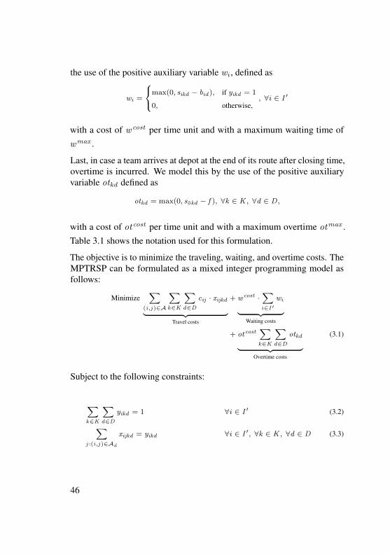
the use of the positive auxiliary variable w

i

, defined as

w

i

=

8<

:max(0, s

ikd

� b

id

), if yikd

= 1

0, otherwise,, 8i 2 I

0

with a cost of wcost per time unit and with a maximum waiting time ofw

max .

Last, in case a team arrives at depot at the end of its route after closing time,overtime is incurred. We model this by the use of the positive auxiliaryvariable ot

kd

defined as

ot

kd

= max(0, sokd

� f ), 8k 2 K , 8d 2 D ,

with a cost of otcost per time unit and with a maximum overtime ot

max .Table 3.1 shows the notation used for this formulation.

The objective is to minimize the traveling, waiting, and overtime costs. TheMPTRSP can be formulated as a mixed integer programming model asfollows:

MinimizeX

(i,j)2A

X

k2K

X

d2D

c

ij

· xijkd

| {z }Travel costs

+ w

cost ·X

i2I

0w

i

| {z }Waiting costs

+ ot

cost

X

k2K

X

d2D

ot

kd

| {z }Overtime costs

(3.1)

Subject to the following constraints:

X

k2K

X

d2D

y

ikd

= 1 8i 2 I

0 (3.2)

X

j :(i,j)2Ad

x

ijkd

= y

ikd

8i 2 I

0, 8k 2 K , 8d 2 D (3.3)

46

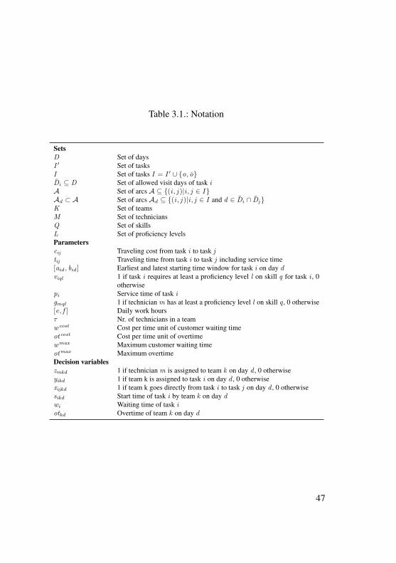
Table 3.1.: Notation

SetsD Set of daysI

0 Set of tasksI Set of tasks I = I

0 [ {o, o}¯

D

i

✓ D Set of allowed visit days of task i

A Set of arcs A ✓ {(i , j )|i , j 2 I }A

d

⇢ A Set of arcs Ad

✓ {(i , j )|i , j 2 I and d 2 ¯

D

i

\ ¯

D

j

}K Set of teamsM Set of techniciansQ Set of skillsL Set of proficiency levelsParametersc

ij

Traveling cost from task i to task j

t

ij

Traveling time from task i to task j including service time[a

id

, bid

] Earliest and latest starting time window for task i on day d

v

iql

1 if task i requires at least a proficiency level l on skill q for task i , 0otherwise

p

i

Service time of task i

g

mql

1 if technician m has at least a proficiency level l on skill q , 0 otherwise[e, f ] Daily work hours⌧ Nr. of technicians in a teamw

cost Cost per time unit of customer waiting timeot

cost Cost per time unit of overtimew

max Maximum customer waiting timeot

max Maximum overtimeDecision variablesz

mkd

1 if technician m is assigned to team k on day d , 0 otherwisey

ikd

1 if team k is assigned to task i on day d , 0 otherwisex

ijkd

1 if team k goes directly from task i to task j on day d , 0 otherwises

ikd

Start time of task i by team k on day d

w

i

Waiting time of task i

ot

kd

Overtime of team k on day d

47

X

j :(o,j)2Ad

x

ojkd

= 1 8k 2 K , 8d 2 D (3.4)

X

i:(i,o)2Ad

x

iokd

= 1 8k 2 K , 8d 2 D (3.5)

X

i:(i,h)2Ad

x

ihkd

�X

j :(h,j)2Ad

x

hjkd

= 0 8h 2 I

0, 8k 2 K , 8d 2 D (3.6)

x

ijkd

(s

ikd

+ t

ij

� s

jkd

) 0 8i , j : (i , j ) 2 Ad

, 8k 2 K ,

8d 2 D (3.7)

y

ikd

(a

id

� s

ikd

) 0 8i 2 I

0, 8k 2 K , 8d 2 D (3.8)

y

ikd

(s

ikd

� b

id

� w

i

) 0 8i 2 I

0, 8k 2 K , 8d 2 D (3.9)

x

ojkd

(s

jkd

� e � t

oj

) � 0 8j 2 I

0, 8k 2 K , 8d 2 D (3.10)

x

iokd

(s

ikd

+ t

io

� f � ot

kd

) 0 8i 2 I

0, 8k 2 K , 8d 2 D (3.11)X

k2K

z

mkd

1 8m 2 M , 8d 2 D (3.12)

X

m2M

z

mkd

= ⌧ 8k 2 K , 8d 2 D (3.13)

v

iql

y

ikd

X

m2M

g

mql

z

mkd

8i 2 I

0, 8q 2 Q , 8l 2 L,

8k 2 K , 8d 2 D (3.14)

0 w

i

w

max 8i 2 I

0 (3.15)

0 ot

kd

ot

max 8k 2 K , 8d 2 D (3.16)

s

ikd

� 0 8i 2 I , 8k 2 K , 8d 2 D (3.17)

x

ijkd

, yikd

, zmkd

2 {0, 1} 8i , j 2 I , 8m 2 M , 8k 2 K ,

8d 2 D (3.18)

Constraints (3.2) and (3.3) ensure that all tasks are assigned exactly onceto one team on any feasible day with respect to the requested visit days.Constraints (3.4) and (3.5) ensure that each team starts and ends its routeat the depot. Constraint (3.6) ensures flow conservation when visiting atask site. Constraint (3.7) allows a task to be started only if its preceding

48

task is completed, which implicitly corresponds to a sub-tour eliminationconstraint. Constraints (3.8) and (3.9) state that a task can only start withinits time window. If a team starts a task after its latest starting time, a penaltyon customer waiting is incurred. Note that constraints (3.7)-(3.9) can belinearized by using a big M formulation. The routes’ duration limit andovertime are defined by constraints (3.10) and (3.11). Constraint (3.12)ensures that a technician is assigned to at most one team per day, andequation (3.13) defines the number of technicians per team. Constraint(3.14) ensures that the skill requirements of task i are fulfilled by thecombination of skills from the technicians assigned to a team. Constraints(3.15) and (3.16) define the bounds for customer waiting and overtime,respectively. Lastly, constraints (3.17) and (3.18) define the positive andthe binary variables, respectively.

From (3.1), constraints (3.2)-(3.11), and (3.15)-(3.18) we observe that theMPTRSP contains, as a special case, the Vehicle Routing Problem withTime Windows (VRPTW) with a fixed fleet size, which is an NP-hardproblem (Solomon, 1987; Solomon and Desrosiers, 1988a). Note that evenfinding a feasible solution to the VRPTW is itself an NP-complete problem(Savelsbergh, 1985). The remaining team building constraints correspondto a special case of the two-to-one assignment problem (2-1-AP) (Goossenset al., 2012) with no cost-coefficients.

3.4. Branch-and-price algorithms

The choice of column generation-based algorithms to solve workforcescheduling and routing problems stems from their similarities with thevehicle routing problem (VRP), on which this method is commonly applied(see, e.g., Desrochers et al. (1992), Kohl and Desrosiers (1999), and Lib-

49

eratore et al. (2010)). This approach exploits the structure of the problemby reformulating is as a master problem (MP) and a pricing problem(s)using, e.g., Danzig-Wolfe decomposition, and provides a fractional lowerbound. To guarantee integrality, column generation can be embeddedin a branch-and-bound algorithm to branch on fractional variables, i.e.,branch-and-price can be applied.

In the MIP formulation for the Multiperiod Technician Routing and Schedul-ing Problem (MTRSP), we observe that (3.2) and (3.3) are the only con-straints that link the teams and days together, whereas the rest are team andday specific. This allows us to apply a similar decomposition and use abranch-and-price algorithm to solve the problem. However, this fact also al-lows a certain degree of flexibility as to which constraints are selected to bein the MP and pricing problem(s). In this section, we illustrate the applica-tion of a branch-and-price algorithm using two alternative decompositionsof the MPTRSP and details on its implementation.

3.4.1. Day decomposition

Exploiting the fact that the time windows spanning several days can berepresented as multiple alternative single-day time windows, the MPTRSPcan be decomposed into a master problem that selects the best routes for allteams on each day in the planning horizon, and single-day pricing problemsfrom which daily technician-to-team assignments and daily routes for allteams are obtained.

As for the MP, let Pd

be the set of feasible schedules containing feasibleroutes (i.e., paths) for all teams on day d and �

dp

be a binary variable equalto 1 on day d schedule p is used, 0 otherwise. Additionally, let ✓

idp

be

50

a parameter equal to 1 if task i on day d is on schedule p, 0 otherwise,and '

ijkdp

be a parameter equal to 1 if arc (i , j ) is used by team k on dayd and schedule p, 0 otherwise. Then, the integer master problem for theday-decomposition (MP-D) can be defined as:

MinimizeX

d2D

X

p2P

d

c

dp

�dp

(3.19)

Subject to:

X

d2D

X

p2P

d

✓idp

�dp

= 1 8i 2 I

0 (3.20)

X

p2P

d

�dp

= 1 8d 2 D (3.21)

�dp

2 {0, 1} 8d 2 D , 8p 2 P

d

(3.22)

Where the cost of a schedule p 2 P

d

is defined by:

c

dp

=

X

k2K

X

i,j :(i,j)2p

c

ij

'ijkd

+ w

cost

X

i2p

w

i

+ ot

cost

X

k2K

ot

kd

(3.23)

The objective is to minimize the overall costs. The set partitioning con-straint (3.20) ensures that tasks are assigned exactly once. Convexityconstraint (3.21) states that exactly one schedule is used per day. Last, con-straint (3.22) defines the binary requirements for the assignment variables.The linear relaxation of this formulation (LMP-D), obtained by relaxingconstraint (3.22), can be used to obtain a lower bound on the MP. However,set P

d

may contain a large number of feasible schedules thus making the so-lution to this problem computationally intractable. Therefore, in a column

51

generation approach, only subset P 0d

⇢ P

d

of schedules, i.e., columns, areconsidered in a restricted master problem (RMP-D). Additional feasiblecolumns are obtained by the iterative solution of a pricing problem, whichconsists of finding schedules with negative reduced cost c

dp

:

c

dp

= c

dp

�X

i2I

0✓idp

⇡i

� ⇢d

(3.24)

=

X

k2K

X

i,j :(i,j)2p

(c

ij

� ⇡i

)'ijkd

+ w

cost

X

i2p

w

i

+ ot

cost

X

k2K

ot

kd

� ⇢d

where ⇡i

, and ⇢d

correspond to the dual values of constraints (3.20) and(3.21) in the optimal solution of the RMP-D.

These values are then passed to the subproblems from which daily schedulesfor all teams are obtained. The pricing problems correspond to a single-dayversion of the original MPTRSP problem (i.e., (3.1)-(3.18), without thed index), one for each day in the planning horizon, which can be solved,e.g., by the use of commercial optimization software. For this, for eachd -subproblem, we let I 0

sub

d

⇢ I

0 and I

sub

d

⇢ I be the set of tasks thatcan be served on day d . Also, we let A

sub

d

= {(i , j )|i , j 2 I

sub

d

} be thecorresponding subnetwork for this subproblem.

This decomposition has the advantage that it can easily incorporate differentteam sizes. However, each pricing problem corresponds to a single-dayMPTRSP (a general case of the VRPTW), which is an NP-hard problem.This may constitute a major drawback for this approach regarding compu-tation time, as column generation involves solving the pricing problemsmultiple times.

52

3.4.2. Team-day decomposition

In addition to decomposing the MPTRSP by days, another possibility is todecompose it by teams. As technician-to-team assignments can change on adaily basis, however, some additional considerations are required. Becausethe workforce composition and team size are known in advance, we canassume without loss of generality that all possible team configurationsare also known. We now let K be the set of all teams resulting fromall possible combinations of all technicians m 2 M in teams of size ⌧size, hence |K| = |M |!

⌧ !(|M |�⌧)! . Therefore, the assignment of techniciansto teams can be pre-defined by letting z

mkd

be a parameter with a valueof 1 if technician m 2 M belongs to team configuration k 2 K on dayd 2 D , and 0 otherwise. Thus the technician-to-team assignments becomeparameters instead of decision variables. In other words, instead of buildingteams (constraints (3.12)-(3.13)), we now address a daily assignment ofpre-configured teams to tasks. This allows us to decompose the MPTRSPinto a master problem defining routes for each team on each day of theplanning horizon and a pricing problem from which daily routes per teamare obtained.

As for the master problem for this decomposition (MP-KD), let Pkd

bethe set of feasible routes (i.e., paths) for team k on day d and �

kdp

be abinary variable equal to 1 only if team configuration k uses path p on dayd . Additionally, let ✓

ikdp

be a parameter equal to 1 if task i is in path p ofteam configuration k on day d , 0 otherwise, '

ijkdp

be a parameter equalto 1 if arc (i , j ) is used by team k on day d and path p, 0 otherwise, and⌘mkdp

be a parameter equal to 1 only if technician m is assigned on thepath p of team configuration k on day d . Then, the MP can be defined as:

53

MinimizeX

k2K

X

d2D

X

p2P

kd

c

kdp

�kdp

(3.25)

Subject to:X

k2K

X

d2D

X

p2P

kd

✓ikdp

�kdp

= 1 8i 2 I

0 (3.26)

X

k2K

X

p2P

kd

⌘mkdp

�kdp

1 8m 2 M , 8d 2 D (3.27)

X

p2P

kd

�kdp

= 1 8k 2 K, 8d 2 D (3.28)

�kdp

2 {0, 1} 8k 2 K, 8d 2 D , 8p 2 P

kd

(3.29)

Where the cost of a path p 2 P

kd

is defined by:

c

kdp

=

X

i,j :(i,j)2p

c

ij

'ijkd

+ w

cost

X

i2p

w

i

+ ot

cost

ot

kd

(3.30)

This MP-KD formulation is fairly similar to the MP-D from Section 3.4.1with the exception of constraint (3.27). Because multiple team configura-tions can include the same technician, constraint (3.27) ensures that eachtechnician is assigned at most once per day. Column generation can be usedto solve the linear relaxation of this set partitioning formulation (LMP-KD),which is obtained by relaxing constraint (3.29). However, as set P

kd

maycontain a large number of columns, only a subset P 0

kd

⇢ P

kd

of paths areconsidered in a restricted version of the master problem (RMP-KD). Furtherfeasible columns are obtained by the iterative solution of pricing problems(one for each team and each day), which consist of finding single-day pathsfor each team with negative reduced cost. For each k � d -subproblem welet I 0

sub

kd

= {i 2 I

0|viql

P

m2M

g

mql

z

mkd

8q 2 Q , 8l 2 L; a

id

6= ?}and I

sub

kd

= I

0sub

kd

[ {o, o} be the set of tasks that can be served on day d

54

and for which team k is qualified. Also, let Asub

kd

= {(i , j )|i , j 2 I

sub

kd

}.A given k � d -subproblem can be formulated as a mixed integer pro-gramming model (we omit the k and d index to simplify the notation) asfollows:

Minimize c

p

=

X

i,j :(i,j)2Asub

(c

ij

� ⇡i

)x

ij

+ w

cost

X

i2I

sub

w

i

+

ot

cost

ot �X

m2M

z

m

�m

� ⇢ (3.31)

Subject to:

X

j2I

sub

x

oj

= 1 (3.32)

X

i2I

sub

x

io

= 1 (3.33)

X

i2I

sub

x

ih

�X

j2I

sub

x

hj

= 0 8h 2 I

0sub

(3.34)

x

ij

(s

i

+ t

ij

� s

j

) 0 8i , j 2 I

sub

(3.35)

a

i

s

i

b

i

+ w

i

8i 2 I

0sub

(3.36)

x

oj

(s

j

� e � t

oj

) � 0 8j 2 I

0sub

(3.37)

x

io

(s

i

+ t

io

� f � ot) 0 8i 2 I

0sub

(3.38)

0 w

i

w

max 8i 2 I

0sub

(3.39)

0 ot ot

max (3.40)

s

i

� 0 8i 2 I

0sub

(3.41)

x

ij

2 {0, 1} 8i , j 2 I

sub

(3.42)

where ⇡i

, �md

, and ⇢kd

correspond to the dual values of constraints (3.26),(3.27), and (3.28) in the optimal solution of the restricted master problem.

55

x

ij

is a binary variable with a value of 1 if the arc (i , j ) is used, and 0otherwise. s

i

and w

i

are positive variables corresponding to the startingtime and the customer waiting time of task i , while ot is a positive variablethat comprises the (possible) overtime incurred in this route. The objectiveis to find a route with a minimum reduced cost (3.31). Constraints (3.32),(3.33), and (3.34) ensure the feasibility of the route. Constraint (3.35)defines the tasks’ starting time, whereas constraint (3.36) ensures that timewindows are respected. If a task starts after its latest starting time, customerwaiting occurs. Constraints (3.37) and (3.38) define the working day limits,and if a team arrives at the depot after closing time, overtime is incurred.Note that constraints (3.35), (3.37), and (3.38) can be linearized using abig M formulation. Constraints (3.39) and (3.40) define the bounds for thewaiting and overtime variables, respectively. Last, positive variables (3.41)and binary variables (3.42) are defined.

These subproblems correspond to an Elementary Shortest Path Problemwith Resource Constraints (ESPPRC). This means, that it is necessary toexplicitly enforce elementary paths as the solution of the subproblems,since the dual values ⇡

i

and ⇢d

associated with a task may lead to negativecost cycles (i.e., subcycles). Note that ESPPRC in graphs with negativecost cycles is strongly NP-hard (Dror, 1994). This could represent a ma-jor drawback for this decomposition, as the number of pricing problemsdepends directly on the number of possible team configurations. Becausein our algorithm we need to solve these subproblems several times, anefficient solution approach is required.

Labeling algorithm In the VRPTW literature, a common approach tosolving the pricing problems is to relax the elementary requirement for paths

56

so that the subproblem changes to a Shortest Path Problem with ResourceConstraints (SPPRC) (See, e.g., Desrochers et al. (1992)). This approachcan be solved efficiently using dynamic programming, although it hasthe disadvantage of weakening the lower bound computed by the column-generation master problem (Bode and Irnich, 2014b). However, severalapproaches successfully apply similar dynamic programming methods toefficiently solve the ESPPRC (Feillet et al., 2004) and the ESPPRC withsoft time windows (Liberatore et al., 2010) because of its ability to providetight lower bounds. In the following, we describe a dynamic programmingapproach similar to the approach proposed by Feillet et al. (2004) to solvethe ESPPRC to optimality. Our approach, similar to Ioachim et al. (1998)and Liberatore et al. (2010), considers time dependent cost (i.e., in the caseof customer waiting and overtime) in addition to elementary paths.

Labeling algorithm overview In the following, we present an overviewof our proposed labeling algorithm (see Algorithm 2). For this, we requirethe following notation: let U

i

and Pi

represent the set of unprocessed andprocessed labels for task i , respectively. These sets allow keeping trackof the creation of labels throughout the algorithm. The process starts bysetting sets U

i

and Pi

to the empty set, by creating the first label Lo

, andby adding it to the unprocessed set. Then, iteratively, the label with theminimum cost is selected from the unprocessed set to look for possibleextensions along its arcs. If feasible, new labels are created by extendingeach selected label along all its connecting arcs to successive tasks, andadded to the unprocessed set. Once no more extensions are possible, thecurrently explored label is added to the processed set. To keep the sizeof these sets tractable, dominance rules are applied to discard labels that

57

cannot lead to an optimal solution. Once all paths arriving at the depot oare obtained and no more unprocessed labels remain, the label with theminimum cost is selected and corresponds to the optimal solution of therespective k � d subproblem. Its corresponding reduced cost is determinedby c = C (T

o

)�P

m2M

z

m

�m

� ⇢. If multiple labels (i.e., columns) arefound with the same minimum reduced cost, and none can be dominated,then all are added to the master problem.

Algorithm 2 Labeling algorithm overviewSet U

i

= Pi

= ? 8i 2 I

sub

Set Lo

= (o,To

= e,C (T

o

) = 0,So

= 0)

Set Uo

= {Lo

}while

Si2I

sub

Ui

6= ? doChoose the label L

m

2S

i2I

sub

Ui

with the minimum cost and removeit from U

m

for all arcs (m, j ) 2 N

sub

doExtend L

m

along arc (m, j ) to create label Lj

using the REF’sif L

j

is feasible thenAdd L

j

to Uj

Apply dominance rules to Uj

and Pj

end ifAdd L

m

to Pm

end forFilter P

o

to find the shortest o � o elementary pathend while

Label setting In short, the objective of the algorithm is to obtain routesfrom o to o for a team on a single day, visiting a subset of the other tasks,such that the reduced cost is minimized. For this purpose, we need to definethe following concepts. A state associated with task i corresponds to apartial path of visited tasks from the depot to i . Each task can be associated

58

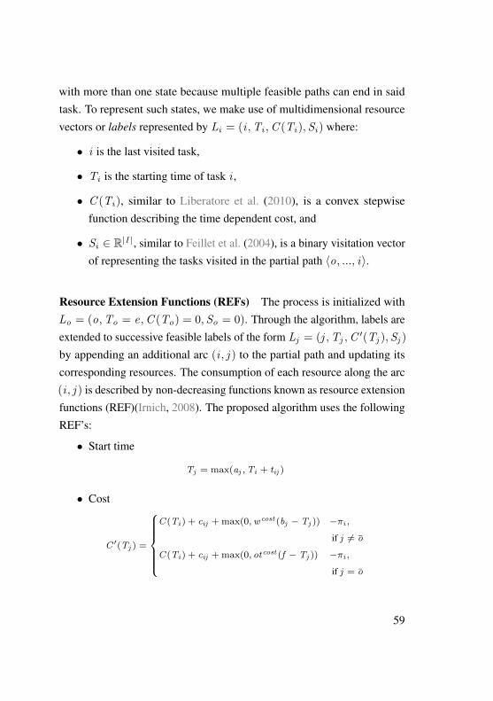
with more than one state because multiple feasible paths can end in saidtask. To represent such states, we make use of multidimensional resourcevectors or labels represented by L

i

= (i ,Ti

,C (T

i

),Si

) where:

• i is the last visited task,

• T

i

is the starting time of task i ,

• C (T

i

), similar to Liberatore et al. (2010), is a convex stepwisefunction describing the time dependent cost, and

• S

i

2 R|I |, similar to Feillet et al. (2004), is a binary visitation vectorof representing the tasks visited in the partial path ho, ..., ii.

Resource Extension Functions (REFs) The process is initialized withL

o

= (o,To

= e,C (T

o

) = 0,So

= 0). Through the algorithm, labels areextended to successive feasible labels of the form L

j

= (j ,Tj

,C 0(T

j

),Sj

)

by appending an additional arc (i , j ) to the partial path and updating itscorresponding resources. The consumption of each resource along the arc(i , j ) is described by non-decreasing functions known as resource extensionfunctions (REF)(Irnich, 2008). The proposed algorithm uses the followingREF’s:

• Start time

T

j

= max(a

j

,Ti

+ t

ij

)

• Cost

C

0(T

j

) =

8>>>>><

>>>>>:

C (T

i

) + c

ij

+max(0,wcost

(b

j

� T

j

)) �⇡i

,

if j 6= o

C (T

i

) + c

ij

+max(0, otcost (f � T

j

)) �⇡i

,

if j = o

59

• Visited tasks

S

j

m

=

8<

:S

j

m

+ 1, if m = j

S

j

m

if m 6= j

The same way as in Feillet et al. (2004) and Liberatore et al. (2010) inorder to enforce elementariness in the path, a dummy resource is associatedwith each task i 2 I such that this resource is consumed when i is visited.That is, S

j

m

= 1 if the path ho, ..., ii visits task m , 0 otherwise. The pathho, ..., ii corresponds to an elementary path only if S

j

m

1 8m 2 I

0sub

.

Feasibility A label (i ,Ti

,C (T

i

),Si

) is feasible if Ti

b

i

+w

max |i 6=o and T

i

b

i

+ ot

max |i = o and is an elementary path. Labels that donot satisfy these conditions are discarded.

Dominance As multiple labels per task are allowed, the ability to discardlabels that do not lead to an optimal solution is crucial for the efficiencyof the algorithm. For this purpose, dominance rules are applied. LetL

i

= (i ,Ti

,C (T

i

),Si

) and L

0i

= (i ,T 0i

,C 0(T

0i

),S 0i

) be two labels of taski . Then, L

i

dominates L0i

if Li

< L

0i

component-wise, i.e., if Ti

T

0i

,C (T

i

) C

0(T

0i

) and S

i

5 S

0i

and at least one of the inequalities is strict.Note that S

i

5 S

0i

means that each element of vector Si

is less than orequal to each corresponding element of vector S 0

i

. If a label is dominatedthen it can be discarded; when all components are equal, both labels arekept.

To strengthen these rules, one can also make use of an additional “reacha-bility” resource, as presented in Feillet et al. (2004). Let U

i

(T

i

) be a binaryresource vector that indicates whether it is feasible to visit other tasks fromtask i given the respective travel and starting times, i.e., if other tasks are

60

reachable from i . This means:

U

i

m

(T

i

) =

8>>>>><

>>>>>:

1, if Si

m

= 1

1, if Ti

+ t

im

> b

i

+ w

max

1, if Ti

+ t

im

> b

i

+ ot

max ,m = o,

0, otherwise

Then, from labels L

i

= (i ,Ti

,C (T

i

),Si

) and L

0i

= (i ,T 0i

,

C

0(T

0i

),S 0i

) with U

i

(T

i

) and U

0i

(T

0i

), the dominance rule S

i

S

0i

can bereplaced by S

i

+ U

i

(T

i

) S

0i

+ U

0i

(T

0i

).

Acceleration strategies The column generation algorithm introduced inthe previous section presents an important drawback in that it requiresthat several ESPPRC subproblems (which are NP-hard) be solved multipletimes for its completion. Solving an ESPPRC to optimality can be compu-tationally expensive, even with our proposed labeling algorithm, when thenumber of tasks increases. It is possible, however, to solve each subprob-lem heuristically since only in the last iteration of the column generationalgorithm an exact solution is required to guarantee optimality (i.e., noadditional columns with negative reduced cost can be found).

In the following, we propose one insertion heuristic and three heuristicsbased on the labeling algorithm previously described. The main idea isto apply these algorithms sequentially during the execution of the columngeneration algorithm. After an initialization phase, the first method is usedto solve each subproblem and pass information to the master problem untilno columns with negative reduced cost are found. Then, the next solutionmethod is chosen, and the process is repeated until no more negativereduced cost columns are found with the last (exact) algorithm. Gendreauet al. (2016) propose a similar approach where a heuristically stopped

61

labeling algorithm and an exact branch-and-cut algorithm are used insequence to solve ESPPRC pricing problems.

Insertion heuristic The column generation is initialized by the use ofa modified version of the insertion heuristic from Solomon (1987). Asthe vehicle “fleet” is not known in advance, we make use of the artificialteams K described at the beginning of this section. This algorithm canbe summarized as follows: (i) for each team k 2 K and day d 2 D ,we sequentially initialize routes by choosing the task with the highesttransportation costs to and from the depot. (ii) For each task h available toteam k on day d , we calculate the operation costs obtained from inserting it,if feasible, in each arc (i , j ) of the initial route. (iii) The insertion (i , h, j )⇤

with the minimum cost is selected, and the initial route is accordinglyupdated. Steps (ii) and (iii) are repeated until no further tasks can beinserted. (iv) The resulting routes are post-processed and inserted as initialcolumns of the reduced master problem. Note that this procedure can stilllead to infeasible schedules, as tasks may remain unassigned. In this case,artificial columns are inserted in the master problem for each unassignedtask.

(H1) Partial pricing Each k � d subproblem focuses on the route of aspecific team on a specific day, and thus, only the tasks corresponding tothis subproblem are considered. Depending on the task time windows oron the skill configuration of the team, it is possible for multiple teams to beassigned to these tasks on the same day with the same route cost. In termsof the column generation procedure, it means that the marginal values �

md

and ⇢kd

have zero values, i.e., there is no prize to earn nor penalty to pay

62

by dispatching team k on day d before other teams on other days. Wecan exploit this fact to reduce the number of subproblems in each iterationby solving only those with marginal values different from zero. In caseno subproblem satisfies this condition, one is selected randomly, and thecolumn generation phase continues.

(H2) Relaxed dominance rules One way to accelerate the solution ofthe subproblems is to relax the dominance rules from the exact labelingalgorithm. This is done by testing the dominance of only a subset ofthe labels’ resource: for two labels L

i

= (i ,Ti

,C (T

i

),S ) and L

0i

=

(i ,T 0i

,C 0(T

0i

),S 0), L

i

dominates L0i

if Ti

T

0i

, C (T

i

) C

0(T

0i

). Theelementariness of the routes is still required, although it is not guaranteedthat an optimal solution is found.

(H3) Partial pricing and partial dominance rules This approach con-sists of a combination of both previously described heuristics: H1 and H2.Therefore, partial pricing is applied in the column generation phase andrelaxed dominance rules are used in the solution of the subproblems.

3.4.3. General procedure

In this section, we outline the proposed branch-and-price algorithm. Itmainly consists of a column generation algorithm embedded in a branch-and-bound procedure to guarantee integrality. Note that the same algorithmis used to solve both decompositions presented in Section 3.4.1 and 3.4.2.Therefore, we now use the terms “master problem” and “pricing problem”

63

generically. Additionally, further details on the implementation of thealgorithm are presented.

Column generation The column generation process can be describedas follows: the algorithm is initialized by the insertion heuristic. Themaster problem is solved with a set of artificial columns obtained by theintroduction of slack variables with a high cost to ensure primal feasibility.Due to their high cost, these variables eventually leave the basis once furtherfeasible columns are obtained. From the solution of the master problem, themarginal values are obtained and passed to the subproblems. New routes(i.e., columns) are obtained by solving the subproblems. If columns arefound with negative reduced cost, the column generation process is startedagain. Otherwise, an optimal solution for the reduced master problem andthus to the master problem is found. If this solution is integer, then it is anoptimal solution for the MPTRSP; if not, it corresponds to a valid fractionallower bound. Otherwise branching on fractional variables is required andcolumn generation is applied on each node with its respective fractionalbounds.

Preprocessing The pricing problems of either decomposition are solvedwith only a subset of the original set of tasks. For each subproblem fromthe day decomposition, only a subset I

sub

d

⇢ I is considered, i.e., the taskswith time windows covering day d . For solving each subproblem of theteam-day-decomposition, only a subset I

sub

kd

⇢ I of tasks is considered;that is, only tasks with a time window covering day d for which constraint(3.14) for the respective k team is fulfilled. If no task satisfies these criteria,

64

i.e., I

sub

d

= ? or Isub

kd

= ?, then the respective pricing problem is notconsidered throughout the column generation phase.

Branching To explore the branching tree a depth-first strategy is used.This allows us to solve each node starting from the feasible solutions foundfor its parent by storing all columns that comply with the current node’sbounds.

Branching on arcs is the branching strategy selected, as branching on the �variables is inefficient and troublesome to implement (Feillet, 2010). Foreach node on the branching tree, we define the set A0 as the set of fractionalarcs (i , j , k , d) such that 0 <

ijkd

< 1, where ijkd

=

Pp2P

d

'ijkdp

�dp

for the day decomposition, and ijkd

=

Pp2P

k

d

'ijkdp

�kdp

for the team-day decomposition. Then, the arc (i , j , k , d)⇤ is selected as:

(i , j , k , d)⇤ 2 argmax

(i,j ,k,d)2A0

�c

ij

·min( ijkd

, 1� ijkd

)

From this node, two successors are generated:

• One node where arc (ijkd)

⇤ is forbidden, i.e., team k cannot visittask j after i on day d . This is done by removing this arc from itsrespective subproblem’s graph, and discard any columns using it.

• Other node where arc (ijkd)

⇤ is fixed, i.e., all other arcs entering j

and leaving i for team k on day d , and all arcs entering i and leavingj for k ‘ 6= k or d 0 6= d are removed so that team k is forced to gofrom i to j on day d . Accordingly, columns using these arcs are thendiscarded from the column pool.

65

3.5. Numerical experiments

For our numerical experiments, we use artificial data generated from knownbenchmarks tests as well as real-world data from a external maintenanceprovider (EMP) to test the performance of the proposed solution approaches.Then, to focus on the impact of the multi-periodicity of the time windows,we conduct a sensitivity analysis varying the length of the time windows.Then, we combine selected test instances to create larger test instances totest the performance of our solution approaches with larger problem sizes.

All solution approaches are implemented in Python 2.7.5 using the Gurobi5.6.2 solver on a 2.5 GHz Intel Core i7 machine with 8 GB RAM. Addition-ally, equations (3.7)-(3.11), (3.35), (3.37), and (3.38) are linearized using abig M formulation, with M =

Pi2I

t

oi

+ t

io

.

3.5.1. Artificial instances

For our first experiments artificial test instances based on known VRPTWbenchmarks (Solomon, 1987) were generated. Instances C101 to C109,R101 to R112, and RC101 to RC108 where selected, where C, R, andRC denote clustered customers, randomly located, and semi-clustered cus-tomers, respectively. From each instance the first 25 customer locations(i.e., tasks) are selected (in addition to the depot) and their allowed visitdays distributed along a 5-day planning horizon in two different variants:first, denoted by suffix a customers’ time windows are defined for a single-day and evenly distributed through the planning horizon (i.e., five tasksper day); second, denoted by suffix b, these customer’s time windowsare extended such that they span two consecutive days cutting off thosewhich exceed the planning horizon’s length. As the goal of these tests is to

66

focus on the impact of the multiperiod time windows on the computationaleffort, no vehicle capacity nor skill requirements are considered, waitingand overtime are not allowed, and routes are limited only by the length ofa working day (defined by the daily time windows of the depot from theoriginal instances). The transportation costs c

ij

correspond to the Euclideandistance between the two customer locations, and the transportation timesare calculated as t

ij

= c

ij

+ p

i

, as in Kohl and Desrosiers (1999). Addi-tionally, we consider a workforce of eight homogeneous technicians andno team building decisions are required. A total of 29 a-instances and 29b-instances were solved setting a time limit of one hour using all three solu-tions methods presented before: the MIP formulation solved by a Gurobi’sbranch-and-cut algorithm, branch-and-price with a day decomposition, andbranch-and-price with a team-day decomposition.

Table 3.2 shows, for the solutions of the MIP formulation obtained byGurobi’s branch-and-cut algorithm, the objective function value, computa-tion time (in minutes) and the relative gap reported by the solver. For eachbranch-and-price method, the objective function value, the computationtime in minutes, the number of nodes explored, the number of columnsgenerated (i.e., number of pricing problems solved), and the absolute gapis shown.

In general, we observe that single day time windows (a-instances) are easierto solve than multiperiod time windows (b-instances), since allowing timewindows to span multiple days increases the time required to solve theproblem. This can be observed by the significant increase in computationtime for either solution method. In addition, we observe that the branch-and-price algorithm with the team-day decomposition needs to exploremore nodes in several cases than with the day decomposition. This implies

67

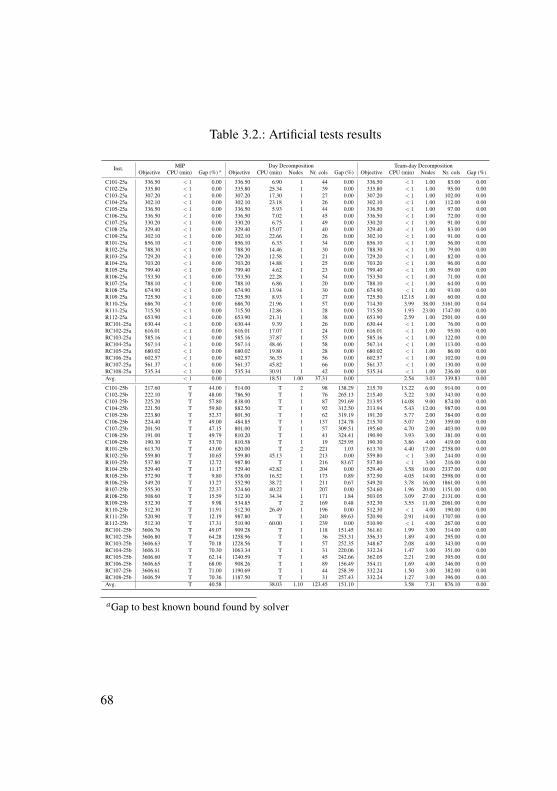
Table 3.2.: Artificial tests results

Inst. MIP Day Decomposition Team-day DecompositionObjective CPU (min) Gap (%) a Objective CPU (min) Nodes Nr. cols Gap (%) Objective CPU (min) Nodes Nr. cols Gap (%)

C101-25a 336.50 < 1 0.00 336.50 6.90 1 44 0.00 336.50 < 1 1.00 83.00 0.00C102-25a 335.80 < 1 0.00 335.80 25.34 1 39 0.00 335.80 < 1 1.00 95.00 0.00C103-25a 307.20 < 1 0.00 307.20 17.30 1 27 0.00 307.20 < 1 1.00 102.00 0.00C104-25a 302.10 < 1 0.00 302.10 23.18 1 26 0.00 302.10 < 1 1.00 112.00 0.00C105-25a 336.50 < 1 0.00 336.50 5.93 1 44 0.00 336.50 < 1 1.00 97.00 0.00C106-25a 336.50 < 1 0.00 336.50 7.02 1 45 0.00 336.50 < 1 1.00 72.00 0.00C107-25a 330.20 < 1 0.00 330.20 6.75 1 49 0.00 330.20 < 1 1.00 91.00 0.00C108-25a 329.40 < 1 0.00 329.40 15.07 1 40 0.00 329.40 < 1 1.00 83.00 0.00C109-25a 302.10 < 1 0.00 302.10 22.66 1 26 0.00 302.10 < 1 1.00 91.00 0.00R101-25a 856.10 < 1 0.00 856.10 6.33 1 34 0.00 856.10 < 1 1.00 56.00 0.00R102-25a 788.30 < 1 0.00 788.30 14.46 1 30 0.00 788.30 < 1 1.00 79.00 0.00R103-25a 729.20 < 1 0.00 729.20 12.58 1 21 0.00 729.20 < 1 1.00 82.00 0.00R104-25a 703.20 < 1 0.00 703.20 14.88 1 25 0.00 703.20 < 1 1.00 96.00 0.00R105-25a 799.40 < 1 0.00 799.40 4.62 1 23 0.00 799.40 < 1 1.00 59.00 0.00R106-25a 753.50 < 1 0.00 753.50 22.28 1 54 0.00 753.50 < 1 1.00 71.00 0.00R107-25a 788.10 < 1 0.00 788.10 6.86 1 20 0.00 788.10 < 1 1.00 64.00 0.00R108-25a 674.90 < 1 0.00 674.90 13.94 1 30 0.00 674.90 < 1 1.00 93.00 0.00R109-25a 725.50 < 1 0.00 725.50 8.93 1 27 0.00 725.50 12.15 1.00 60.00 0.00R110-25a 686.70 < 1 0.00 686.70 21.96 1 57 0.00 714.30 3.99 38.00 3161.00 0.04R111-25a 715.50 < 1 0.00 715.50 12.86 1 28 0.00 715.50 1.93 23.00 1747.00 0.00R112-25a 653.90 < 1 0.00 653.90 21.31 1 38 0.00 653.90 2.59 1.00 2501.00 0.00RC101-25a 630.44 < 1 0.00 630.44 9.39 1 26 0.00 630.44 < 1 1.00 76.00 0.00RC102-25a 616.01 < 1 0.00 616.01 17.07 1 24 0.00 616.01 < 1 1.00 95.00 0.00RC103-25a 585.16 < 1 0.00 585.16 37.87 1 55 0.00 585.16 < 1 1.00 122.00 0.00RC104-25a 567.14 < 1 0.00 567.14 48.46 1 58 0.00 567.14 < 1 1.00 113.00 0.00RC105-25a 680.02 < 1 0.00 680.02 19.80 1 28 0.00 680.02 < 1 1.00 86.00 0.00RC106-25a 602.57 < 1 0.00 602.57 36.35 1 56 0.00 602.57 < 1 1.00 102.00 0.00RC107-25a 561.37 < 1 0.00 561.37 45.82 1 66 0.00 561.37 < 1 1.00 130.00 0.00RC108-25a 535.34 < 1 0.00 535.34 30.91 1 42 0.00 535.34 < 1 1.00 236.00 0.00Avg. < 1 0.00 18.51 1.00 37.31 0.00 2.54 3.03 339.83 0.00

C101-25b 217.60 T 44.00 514.00 T 2 98 138.29 215.70 13.22 6.00 914.00 0.00C102-25b 222.10 T 48.00 786.50 T 1 76 265.13 215.40 5.22 3.00 343.00 0.00C103-25b 225.20 T 57.80 838.00 T 1 87 291.69 213.95 14.08 9.00 874.00 0.00C104-25b 221.50 T 59.80 882.50 T 1 92 312.50 213.94 5.43 12.00 987.00 0.00C105-25b 223.80 T 52.37 801.50 T 1 62 319.19 191.20 5.77 2.00 384.00 0.00C106-25b 224.40 T 49.00 484.85 T 1 137 124.78 215.70 5.07 2.00 359.00 0.00C107-25b 201.50 T 47.15 801.00 T 1 57 309.51 195.60 4.70 2.00 403.00 0.00C108-25b 191.00 T 49.79 810.20 T 1 41 324.41 190.90 3.93 3.00 381.00 0.00C109-25b 190.30 T 53.70 810.58 T 1 19 325.95 190.30 3.86 4.00 419.00 0.00R101-25b 613.70 T 43.00 620.00 T 2 221 1.03 613.70 4.40 17.00 2758.00 0.00R102-25b 559.80 T 10.65 559.80 45.13 1 213 0.00 559.80 < 1 3.00 244.00 0.00R103-25b 537.80 T 12.72 987.80 T 1 216 83.67 537.80 < 1 3.00 216.00 0.00R104-25b 529.40 T 11.17 529.40 42.82 1 204 0.00 529.40 3.58 10.00 2337.00 0.00R105-25b 572.90 T 9.80 578.00 16.52 1 173 0.89 572.90 4.05 14.00 2598.00 0.00R106-25b 549.20 T 13.27 552.90 38.72 1 211 0.67 549.20 3.78 16.00 1861.00 0.00R107-25b 555.30 T 22.37 524.60 40.22 1 207 0.00 524.60 1.96 20.00 1151.00 0.00R108-25b 508.60 T 15.59 512.30 34.34 1 171 1.84 503.05 3.09 27.00 2131.00 0.00R109-25b 532.30 T 9.98 534.85 T 2 169 0.48 532.30 3.55 11.00 2061.00 0.00R110-25b 512.30 T 11.91 512.30 26.49 1 196 0.00 512.30 < 1 4.00 190.00 0.00R111-25b 520.90 T 12.19 987.80 T 1 240 89.63 520.90 2.91 14.00 1707.00 0.00R112-25b 512.30 T 17.31 510.90 60.00 1 239 0.00 510.90 < 1 4.00 267.00 0.00RC101-25b 3606.76 T 49.07 909.28 T 1 118 151.45 361.61 1.99 3.00 314.00 0.00RC102-25b 3606.80 T 64.28 1258.96 T 1 36 253.31 356.33 1.89 4.00 295.00 0.00RC103-25b 3606.63 T 70.18 1228.56 T 1 57 252.35 348.67 2.08 4.00 343.00 0.00RC104-25b 3606.31 T 70.30 1063.34 T 1 31 220.06 332.24 1.47 3.00 351.00 0.00RC105-25b 3606.60 T 62.14 1240.59 T 1 45 242.66 362.05 2.21 2.00 395.00 0.00RC106-25b 3606.65 T 68.00 908.26 T 1 89 156.49 354.11 1.69 4.00 346.00 0.00RC107-25b 3606.61 T 71.00 1190.69 T 1 44 258.39 332.24 1.50 3.00 382.00 0.00RC108-25b 3606.59 T 70.36 1187.50 T 1 31 257.43 332.24 1.27 3.00 396.00 0.00Avg. T 40.58 38.03 1.10 123.45 151.10 3.58 7.31 876.10 0.00

aGap to best known bound found by solver

68

that the team-day decomposition provides a worse linear lower boundthus requiring additional branching in order to close the integer optimalitygap. This observation indicates that we face a trade-off by choosing adecomposition with smaller, easier-to-solve pricing problems but whichmay require more iterations to provide integer solutions.

We also observe that, for the a-instances the team-day decomposition on allits variants is clearly outperformed by the other two exact solution methods.That is because the team-day decomposition considers many subproblemswhich could be aggregated due to the workforce homogeneity (see e.g.,R109-25a to R112-25a). This, however, is not the case for the b-instancesas the team-day decomposition shows the best performance among thesolution approaches regarding computation and solution time. For instance,with the team-day decomposition all instances could be solved to optimalitycompared to only 7 and none with the day decomposition and the MIPformulation, respectively.

3.5.2. Real-world instances

In order to test for performance under real settings, we solve real-worldinstances with three solution methods: solving the MIP formulation directlyGurobi’s branch-and-cut algorithm, the branch-and-price approach with aday decomposition, and the branch-and-price approach with a team-daydecomposition. The data consist of 44 instances, each corresponding to themaintenance requests of a single week. For each task, information such asthe customer location, service time, time windows, and skill requirementswere provided by the company. A total of 66 different customers are consid-ered, and the estimated traveling time to each of their location corresponds

69

to the total travel time of the recommended driving route obtained fromthe Google Maps API (Google, 2016). Note that, since this route includeschanges in elevation due to the topography of the respective area, the dis-tance between locations is not Euclidean. Table 3.3 shows a summary ofthe characteristics (number of tasks, min., max., and avg. service time,min., max., and avg. time window length, max. number of time windows,and number of tasks with multiple time windows) from the consideredinstances. The maintenance provider’s staff consists of six techniciansqualified in five skill domains with three possible proficiency levels pairedinto teams of size ⌧ = 2. In addition, based on maintenance contractsand financial information from the company, the following cost parametersare considered: w

cost

= 300, otcost = 40, and c

ij

= 60 · tij

+ p

i

inmonetary units. Finally, regarding customer waiting and overtime limits,the maintenance provider uses wmax

= ot

max

= 2 hours.

In Table 3.4, the results obtained within a time limit of three hours for allmethods are shown. For each method, the objective value (in monetaryunits), the computation time (in minutes), and the optimality gap is pre-sented for each of the test instances. Note that for the case of the MIP solversolutions, this column shows the gap to the best bound found by the solverwithin the given time limit. For the methods involving branch-and-price,the number of explored nodes while branching and the number of columnsare also shown. In case the time limit is reached (denoted with a “T”), thebest integer solution found is shown. If no integer solution could be found,we report the integer upper bound of the reduced master problem with thecolumns found until reaching the time limit.

From these results, we can make several observations. First, the MIP solveris able to solve only 18 instances to optimality, while in 26 cases, the

70

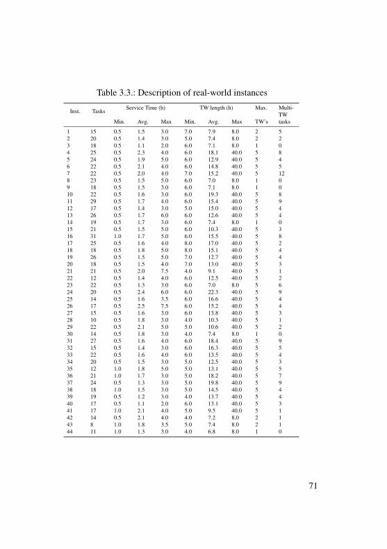
Table 3.3.: Description of real-world instances

Inst. Tasks Service Time (h) TW length (h) Max. Multi-TW

Min. Avg. Max Min. Avg. Max TW’s tasks

1 15 0.5 1.5 3.0 7.0 7.9 8.0 2 52 20 0.5 1.4 3.0 5.0 7.4 8.0 2 23 18 0.5 1.1 2.0 6.0 7.1 8.0 1 04 25 0.5 2.3 4.0 6.0 18.1 40.0 5 85 24 0.5 1.9 5.0 6.0 12.9 40.0 5 46 22 0.5 2.1 4.0 6.0 14.8 40.0 5 57 22 0.5 2.0 4.0 7.0 15.2 40.0 5 128 23 0.5 1.5 5.0 6.0 7.0 8.0 1 09 18 0.5 1.5 3.0 6.0 7.1 8.0 1 010 22 0.5 1.6 3.0 6.0 19.3 40.0 5 811 29 0.5 1.7 4.0 6.0 15.4 40.0 5 912 17 0.5 1.4 3.0 5.0 15.0 40.0 5 413 26 0.5 1.7 6.0 6.0 12.6 40.0 5 414 19 0.5 1.7 3.0 6.0 7.4 8.0 1 015 21 0.5 1.5 5.0 6.0 10.3 40.0 5 316 31 1.0 1.7 5.0 6.0 15.5 40.0 5 817 25 0.5 1.6 4.0 8.0 17.0 40.0 5 218 18 0.5 1.8 5.0 8.0 15.1 40.0 5 419 26 0.5 1.5 5.0 7.0 12.7 40.0 5 420 18 0.5 1.5 4.0 7.0 13.0 40.0 5 321 21 0.5 2.0 7.5 4.0 9.1 40.0 5 122 12 0.5 1.4 4.0 6.0 12.5 40.0 5 223 22 0.5 1.3 3.0 6.0 7.0 8.0 5 624 20 0.5 2.4 6.0 6.0 22.3 40.0 5 925 14 0.5 1.6 3.5 6.0 16.6 40.0 5 426 17 0.5 2.5 7.5 6.0 15.2 40.0 5 427 15 0.5 1.6 3.0 6.0 13.8 40.0 5 328 10 0.5 1.8 3.0 4.0 10.3 40.0 5 129 22 0.5 2.1 5.0 5.0 10.6 40.0 5 230 14 0.5 1.8 3.0 4.0 7.4 8.0 1 031 27 0.5 1.6 4.0 6.0 18.4 40.0 5 932 15 0.5 1.4 3.0 6.0 16.3 40.0 5 533 22 0.5 1.6 4.0 6.0 13.5 40.0 5 434 20 0.5 1.5 3.0 5.0 12.5 40.0 5 335 12 1.0 1.8 5.0 5.0 13.1 40.0 5 536 21 1.0 1.7 3.0 5.0 18.2 40.0 5 737 24 0.5 1.3 3.0 5.0 19.8 40.0 5 938 18 1.0 1.5 3.0 5.0 14.5 40.0 5 439 19 0.5 1.2 3.0 4.0 13.7 40.0 5 440 17 0.5 1.1 2.0 6.0 13.1 40.0 5 341 17 1.0 2.1 4.0 5.0 9.5 40.0 5 142 14 0.5 2.1 4.0 4.0 7.2 8.0 2 143 8 1.0 1.8 3.5 5.0 7.4 8.0 2 144 11 1.0 1.3 3.0 4.0 6.8 8.0 1 0

71

computation time limit is reached. For these cases, the objective valueshows a relatively high gap to the best bound found by the solver (averageof 12%), although in some cases the solution found is the optimal solution(e.g., instances 18, 32, 36, and 39). In the 18 instances with 0% gap, thebranch-and-cut procedure from the solver found the optimal solution inless than one minute, with the exception of instances 22, 25, 26, and 40where the optimal solution was found in 0.2, 4.7, 36.8, and 3.1 minutes,respectively. This indicates that the commercial solver spends ta great dealof time on proving this solution’s optimality.

Second, the branch-and-price with a day decomposition is clearly outper-formed by the other two methods. Within the set time limit only in 13cases, an optimal solution is reported and no feasible solution for instance24 is found. For all of the remaining 40 instances where the computationtime limit is reached, the algorithm stopped during the column generationphase at the root node. The solutions reported correspond to the integersolution of the reduced master problem using the columns obtained upuntil the time of interruption, which explains the reason why the optimalitygap is so high in some cases (see, e.g., instance 11, 24, and 10). This lowperformance is due to the high computational effort required to solve thepricing problems in the day decomposition. Furthermore, the frequencywith which the pricing problems are solved has an important impact on theperformance. In the case of instances with tasks with none or few multipletime windows, the computation time is low since tasks can be assigned tofew possible validity periods, thus, few iterations of the column generationphase are required. On the other hand, instances with high number oftasks with multiple periods require more time to solve as the number ofcombinations of possible validity days increases, thus greatly incrementing

72

the number of iterations of the column generation phase. However, weobserve that using this decomposition has the advantage that it providesbetter bounds than the team-day decomposition, as in all the cases wherean optimal solution is obtained, it is found at the root node. Thus, there is aclear trade-off between the computational effort spent into solving largerpricing problems and the savings while exploring the branching tree due totighter bounds.

Third, the team-day decomposition clearly outperforms the other solutionmethods, because it is able to find a proven optimal solution for all casesin an acceptable computation time. With a maximum of 16.25 minutes,the team-day-decomposition solves this weekly planning problem for allinstances to optimality in short time.

3.5.3. Impact of the length of the time windows

The purpose of the following experiments is manyfold: we further test theperformance of our algorithms with additional test instances, and we testthe impact of the time window length on the objective function value andcomputation time. Note that we refer to window length as the number ofdays covered by a single time window, and not exclusively the number ofperiods covered by it. For this purpose, we generate 45 test instances byselecting different instances from Section 3.5.2, and multiplying their timewindow length by a scaling factor in the interval [0, 2]. The nine selectedweeks correspond to the instances with:

• Type A: Min., max., and average time window length (Week 44, 24,and 13, respectively).

73

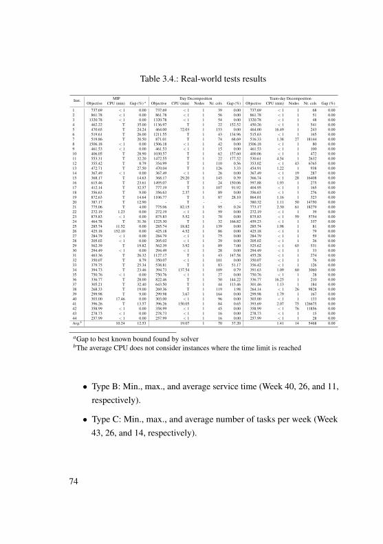
Table 3.4.: Real-world tests results

Inst. MIP Day Decomposition Team-day DecompositionObjective CPU (min) Gap (%) a Objective CPU (min) Nodes Nr. cols Gap (%) Objective CPU (min) Nodes Nr. cols Gap (%)

1 737.69 < 1 0.00 737.69 < 1 1 39 0.00 737.69 < 1 1 68 0.002 861.78 < 1 0.00 861.78 < 1 1 56 0.00 861.78 < 1 1 51 0.003 1320.78 < 1 0.00 1320.78 < 1 1 54 0.00 1320.78 < 1 1 48 0.004 462.22 T 35.00 1136.97 T 1 22 152.52 450.26 < 1 1 541 0.005 470.65 T 24.24 464.00 72.03 1 153 0.00 464.00 16.49 1 243 0.006 519.61 T 26.00 1211.55 T 1 43 134.96 515.63 < 1 1 165 0.007 519.86 T 20.50 871.01 T 1 74 68.69 516.33 1.38 27 18144 0.008 1506.18 < 1 0.00 1506.18 < 1 1 42 0.00 1506.18 < 1 1 80 0.009 461.53 < 1 0.00 461.53 < 1 1 15 0.00 461.53 < 1 1 100 0.0010 406.05 T 28.90 1030.57 T 1 62 157.60 400.06 < 1 1 472 0.0011 553.31 T 32.20 1472.55 T 1 22 177.52 530.61 4.54 1 2632 0.0012 355.42 T 8.79 354.99 T 1 110 0.56 353.02 < 1 43 6765 0.0013 472.71 T 27.50 470.04 T 1 126 3.33 454.91 1.22 1 938 0.0014 367.49 < 1 0.00 367.49 < 1 1 26 0.00 367.49 < 1 19 287 0.0015 368.17 T 14.63 368.17 29.20 1 145 0.39 366.74 < 1 28 16408 0.0016 615.46 T 23.61 1495.07 T 1 24 150.06 597.88 1.93 1 275 0.0017 412.14 T 32.57 777.19 T 1 107 91.92 404.95 < 1 1 165 0.0018 356.63 T 9.00 356.63 2.37 1 89 0.00 356.63 < 1 1 276 0.0019 872.63 T 14.64 1106.77 T 1 87 28.10 864.01 1.16 1 323 0.0020 387.17 T 12.90 - T - - - 380.32 1.11 50 14750 0.0021 775.06 T 4.00 775.06 82.15 1 95 0.24 773.17 2.30 61 18279 0.0022 272.19 1.23 0.00 272.19 < 1 1 59 0.00 272.19 < 1 1 39 0.0023 875.83 < 1 0.00 875.83 5.52 1 70 0.00 875.83 < 1 59 5754 0.0024 464.78 T 31.36 1225.30 T 1 32 166.82 459.23 < 1 1 337 0.0025 285.74 11.52 0.00 285.74 18.82 1 139 0.00 285.74 1.98 1 81 0.0026 425.18 152.10 0.00 425.18 4.52 1 86 0.00 425.18 < 1 1 79 0.0027 284.79 < 1 0.00 284.79 < 1 1 75 0.00 284.79 < 1 1 59 0.0028 205.02 < 1 0.00 205.02 < 1 1 29 0.00 205.02 < 1 1 26 0.0029 562.39 T 19.82 562.39 3.92 1 89 7.00 525.62 < 1 65 531 0.0030 294.49 < 1 0.00 294.49 < 1 1 28 0.00 294.49 < 1 1 33 0.0031 463.36 T 26.32 1127.17 T 1 43 147.58 455.28 < 1 1 274 0.0032 350.07 T 8.79 350.07 < 1 1 101 0.00 350.07 < 1 1 76 0.0033 379.75 T 25.34 538.81 T 1 83 51.17 356.42 < 1 1 126 0.0034 394.73 T 23.46 394.73 137.54 1 109 0.79 391.63 1.09 60 3060 0.0035 750.76 < 1 0.00 750.76 < 1 1 27 0.00 750.76 < 1 1 28 0.0036 336.77 T 28.00 822.46 T 1 50 144.22 336.77 16.25 1 210 0.0037 305.21 T 32.40 643.50 T 1 44 113.46 301.46 1.13 1 184 0.0038 268.33 T 19.00 269.36 T 1 119 1.98 264.14 < 1 26 9828 0.0039 299.98 T 9.00 299.98 3.67 1 164 0.00 299.98 1.79 1 167 0.0040 303.00 17.46 0.00 303.00 < 1 1 96 0.00 303.00 < 1 1 133 0.0041 396.26 T 13.57 396.26 150.05 1 84 0.65 393.69 2.07 75 126675 0.0042 358.99 < 1 0.00 358.99 < 1 1 45 0.00 358.99 < 1 76 11856 0.0043 278.73 < 1 0.00 278.73 < 1 1 16 0.00 278.73 < 1 1 15 0.0044 257.99 < 1 0.00 257.99 < 1 1 16 0.00 257.99 < 1 1 28 0.00Avg.b 10.24 12.53 19.07 1 70 37.20 1.41 14 5468 0.00

aGap to best known bound found by solverbThe average CPU does not consider instances where the time limit is reached

• Type B: Min., max., and average service time (Week 40, 26, and 11,respectively).

• Type C: Min., max., and average number of tasks per week (Week43, 26, and 14, respectively).

74

If the working day length is exceeded, a new time window is started on thenext consecutive day. In case the length of the planning horizon is exceeded,the length of the last time window is cut out. To solve these instances, weselect the team-day decomposition, as it shows the best performance in theresults from previous tests.

Figures 3.1 and 3.2 show the objective function value and computation timeresulting from each scaling factor for each of the selected instances. Inthese graphs, we observe the following effects. First, the overall costs aredecreasing when increasing the time window length. The wider the timewindows get, the lower their impact is on the reduction of overall costs.Second, we observe an increase in the computation time of all instanceswhen increasing the time window length. Since these effects can also beobserved in single-period time windows, the observed results show thatthe same behavior can be expected in the multi-period case. Nevertheless,these effects did not present the same magnitude in all instances (see e.g.,C avg. and C max.). This can be explained by the fact that the selectedweeks show a high number of multiple requests per customer, i.e., thereare significantly more tasks than locations to visit, which results in highsymmetry.

3.5.4. Performance with larger instances

To further test the performance of our solution methods, we generatelarger artificial instances from the afore-described real-world data. Threeinstances were obtained by combining the demand of three different weeksand tripling the workforce. Each instance is generated by combining weeks(I) A min., A avg., and A max., (II) B min., B avg., and B max., and (III) C

75

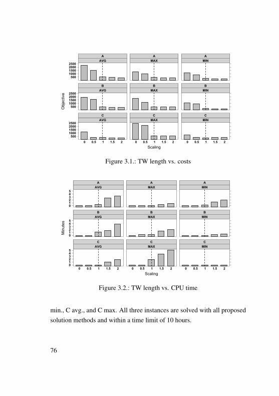
Scaling

Objective

5001000150020002500

AVGA

MAXA

MINA

5001000150020002500

AVGB

MAXB

MINB

5001000150020002500

0 0.5 1 1.5 2

AVGC

0 0.5 1 1.5 2

MAXC

0 0.5 1 1.5 2

MINC

Figure 3.1.: TW length vs. costs

Scaling

Minutes

012345

AVGA

MAXA

MINA

012345

AVGB

MAXB

MINB

012345

0 0.5 1 1.5 2

AVGC

0 0.5 1 1.5 2

MAXC

0 0.5 1 1.5 2

MINC

Figure 3.2.: TW length vs. CPU time

min., C avg., and C max. All three instances are solved with all proposedsolution methods and within a time limit of 10 hours.

76

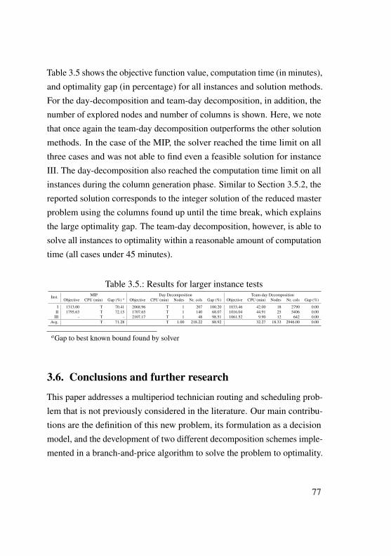
Table 3.5 shows the objective function value, computation time (in minutes),and optimality gap (in percentage) for all instances and solution methods.For the day-decomposition and team-day decomposition, in addition, thenumber of explored nodes and number of columns is shown. Here, we notethat once again the team-day decomposition outperforms the other solutionmethods. In the case of the MIP, the solver reached the time limit on allthree cases and was not able to find even a feasible solution for instanceIII. The day-decomposition also reached the computation time limit on allinstances during the column generation phase. Similar to Section 3.5.2, thereported solution corresponds to the integer solution of the reduced masterproblem using the columns found up until the time break, which explainsthe large optimality gap. The team-day decomposition, however, is able tosolve all instances to optimality within a reasonable amount of computationtime (all cases under 45 minutes).

Table 3.5.: Results for larger instance testsInst. MIP Day Decomposition Team-day Decomposition

Objective CPU (min) Gap (%) a Objective CPU (min) Nodes Nr. cols Gap (%) Objective CPU (min) Nodes Nr. cols Gap (%)

I 1313.00 T 70.41 2068.96 T 1 207 100.20 1033.46 42.00 18 2790 0.00II 1795.63 T 72.15 1707.65 T 1 140 68.07 1016.04 44.91 25 5406 0.00

III - T - 2107.17 T 1 48 98.51 1061.52 9.90 12 642 0.00Avg. T 71.28 T 1.00 218.22 88.92 32.27 18.33 2946.00 0.00

aGap to best known bound found by solver

3.6. Conclusions and further research

This paper addresses a multiperiod technician routing and scheduling prob-lem that is not previously considered in the literature. Our main contribu-tions are the definition of this new problem, its formulation as a decisionmodel, and the development of two different decomposition schemes imple-mented in a branch-and-price algorithm to solve the problem to optimality.

77

These solution approaches are further tested with data from an externalmaintenance provider (EMP).

The results of our tests show that our solution approaches are able to solvethe majority of instances for this complex problem to optimality within anacceptable amount of time. However, we observe that this performancegreatly depends on the selected decomposition scheme used in the branch-and-price algorithm. On the one hand, using a decomposition with fewer,harder-to-solve subproblems provides tighter fractional lower bounds, al-though it is computationally more expensive. On the other hand, using adecomposition with more, easier-to-solve subproblems may result in worsefractional lower bounds, although it allows us to obtain optimal solutionsfor all of our test instances in a shorter amount of time. This also holds forlarger problem instances, as our experiments indicate. Furthermore, oursensitivity analysis shows that additional flexibility, in the form of length(and number) of time windows, has a direct impact on operations costs.This fact needs to be considered during maintenance contract negotiations.

Further research needs to be conducted to incorporate our current decisionmodel as part of a hierarchical planning process such that, as a first step,the weekly plans obtained through our approaches are used to announcevisit times to customers. As a second step, the EMP management wouldoversee the execution of these plans on a daily basis and adjust them in caseunforeseen events occur. Additionally, other features such as technicians’preferences, planned meal breaks, balanced workloads, etc. can also beincluded. As for the proposed solution methods, further research is neededto improve their performance by applying ideas used in the VRP literaturefor this purpose, e.g., relaxation of the subproblems, applying cuts inthe branching trees, other branching strategies, stabilization strategies,

78

intensification strategies, etc. Additionally, other hybrid and heuristicapproaches could be adapted for this problem.

Acknowledgements

This research was supported by the Erich-Becker-Stiftung, a foundation ofFraport AG. The authors are grateful to the anonymous referees for helpfuland constructive suggestions.

79

4. Task assignment with start time-dependentprocessing times for personnel at check-incounters

Co-authors:

Annika Becker and Raik StolletzChair of Production Management, Business School, University ofMannheim, Germany

Working paper, under consideration for publication.

Abstract:

This paper addresses a task-assignment problem encountered by check-incounter personnel at airports. The problem consists of assigning multi-skilled agents to a sequence of tasks in check-in counters. Because eachtask’s ending time is fixed to comply with the flight schedule, its pro-cessing time depends on the arrival of the assigned agents. We proposea mixed-integer program and a branch-and-price algorithm to solve thisproblem. We exploit the problem structure to efficiently formulate thepricing problems and improve computation time. Using real-world datafrom a German ground-handling agency, we conduct numerical studies toevaluate the performance of the proposed solutions.

81

4.1. IntroductionThis paper addresses a task assignment problem encountered by ground-handling agencies at airports, where employees are assigned to processflight check-ins and boardings (i.e., tasks). Because these agencies providethe manpower required for multiple airlines’ flights, they need to ensurethat sufficient staff is available in a timely fashion for all flights; otherwise,they may incur penalties for violating their contracts with the airlines.Furthermore, as 66% to 75% of a ground-handling agency’s operation costscorrespond to personnel costs (Steer Davies Gleave, 2010), inadequateworkforce plans (e.g., overstaffing) are highly undesirable.

The basic structure of a ground-handling agency’s workforce planningprocess can be divided into four planning stages (Stolletz, 2010): (i) headcount planning, (ii) tour scheduling, (iii) task assignment, and (iv) replan-ning. Our work addresses the third stage of this process, during which tasksare assigned to employees on a daily basis taking into account the agent’sskills and availability, traveling time between counters, flight schedules,and contract conditions with the airlines. The specific characteristics of thepresent problem are described below.

The demand for agents is caused by both the flight schedules and the con-tracts between the airlines and the ground-handling agencies. The flightschedules provide daily flight-departure times and therefore, the timeswhen demand occurs. They also provide information about the assignmentof flights to counters, which in turn implies that the transportation timebetween the tasks’ locations is known. The contracts with the airlines de-termine the agent requirements (i.e., number of agents and skills required),along with the counters’ opening and closing times for processing tasks.As can be observed in practice, agents are allowed to arrive at a counter

82

after its opening time, albeit at a cost, because this tardiness is penalized inthe contracts with the airlines. Regardless of an agent’s tardiness, however,he or she is required to remain at the assigned counter until its closing time.This means that all tasks’ end times are fixed and, thus, their duration isdependent on the assigned agent’s arrival times.

The following issues are taken into consideration when managing theground-handler’s workforce. First, agent availability is derived from theshift schedules and days-off schedules obtained in the preceding planningstage, i.e., tour scheduling. As explained in Stolletz (2010) and Stolletz andZamorano (2014), shifts can have varying durations, can start at differenthours of the day, and can vary from day to day. Although shift-planningdecisions cannot be influenced by the task assignment, overtime is allowedif the completion of the final task fulfilled exceeds the length of the shift(which is subject to labor regulations). Second, agents are qualified to oper-ate various airlines’ check-in systems, i.e., the workforce is multiskilled,and they may change the check-in system in which they are working dur-ing the course of a shift. Neither hierarchical skills nor proficiency levelsare considered. If no employee is available to process a task, a limitednumber of fully qualified supervisors and/or management personnel canbe ”outsourced” from the back office to cover the demand, although this isundesirable because it distracts the supervisors and managers from theirnormal responsibilities.

The goal of this planning problem is to obtain daily schedules consisting oftask assignments for each agent for a planning horizon of one day. Theseassignments define a sequence of tasks for each agent, because the tasks’end times are fixed. Additionally, these schedules need to minimize theweighted sum of traveling time, overtime, outsourced time, and tardiness.

83

The contribution of this paper is manifold:

• We address a new task assignment problem that incorporates variabletask duration and fixed end time;

• We propose an exact branch-and-price solution approach to solvethis problem in short computation time; and

• We test our proposed approach with real-world data.

The remainder of the paper is organized as follows. In Section 4.2, relatedliterature on similar task assignment problems is presented. The taskassignment process for check-in counters is explained in detail and thealgebraic notation of the mixed-integer programming model is presented inSection 4.3. In Section 4.4, the branch-and-price algorithm is described. InSection 4.5, the numerical analysis of a real-world example is conducted.Conclusions and directions for further research are presented in Section4.6.

4.2. Literature review

This paper addresses a problem that can be classified into different streamsof literature because of the different features associated with various appli-cations of the problem. The allocation of tasks to agents corresponds to taskassignment problems, although the consideration of changeover times (ortraveling time) is also related to routing problems. In the following section,we present a comparison of the related literature from different applicationareas of task assignment, task scheduling, and routing problems, describingsimilarities and differences compared to the presented problem.

84

Task assignment problems are addressed in several workforce-planningsettings. Generally, task assignment (also referred to as task allocation)consists of assigning a particular number of employees to perform a partic-ular number of tasks (Edison and Shima, 2011). Typically, such problemsinvolve the mere allocation of employees to tasks (see, e.g., Liang andBuclatin, 1988; Miller and Franz, 1996; Campbell, 1999; Campbell andDiaby, 2002; Krishnamoorthy et al., 2012; Liu et al., 2013; Smet et al.,2014). During the last decade, research has generally not addressed taskassignment problems but has focused on task scheduling problems.

In task scheduling problems, both the assignment of employees to tasks andthe start time of a task are part of the decision. Optionally, there could be atime window during which an employee is allowed to start a task. In theseproblems, the processing time is given as input and it can be consideredeither fixed or employee-dependent. In either case, this means that the endtimes of the tasks become dependent variables.

Loucks and Jacobs (1991), Corominas et al. (2006), Cordeau et al. (2010b),and Lieder et al. (2015) provide examples of task-scheduling literature thatassumes fixed task durations, albeit without considering routing decisions.Conversely, Li et al. (2005), Eveborn et al. (2006a), Dohn et al. (2009a),and Kovacs et al. (2012) include routing in their models. Dohn et al. (2009a)address a decision problem similar to ours regarding ground personnel atairports. In their model, employees with different skills are assigned totasks (e.g., baggage handling, check-ins, ticketing). As in our model, tasksmay require more than one agent for their completion, based on the taskrequirements. Unlike our model, all of the agents assigned to a task areforced to start it at the same time (i.e., no tardiness is allowed). The authors

85

propose a branch-and-price approach to solve this problem and test it usingreal-world data from a European airport.

Other studies in the task-scheduling literature assume that the duration of atask (i.e., processing time) depends on the employee fulfilling the task. Themodels of Corominas et al. (2010) and Olivella et al. (2013) assume thatthe duration of a task depends on the worker’s experience and that futureperformance of the task can be increased. However, these two modelsdo not include routing. With respect to similar applications that includerouting, Caseau and Koppstein (1992) present an approach to solve thetechnician-assignment problem in the telephone industry, assuming that theduration of a task depends on the efficiency ratio based on the technician’sskills. Yang (1996) and Tsang and Voudouris (1997) provide solutionsto the workforce management problem at British Telecom. Engineersare allocated to jobs taking into account that job duration depends on theengineer’s effectiveness rate and skill level, respectively.

Table 4.1 summarizes previous research based on the characteristics ofthe tasks. A task’s starting time, processing time, and ending time maybe inputs for the various decision models, decision variables or dependentdecision variables. The assignment of an employee to a task is the maindecision variable.

Existing task assignment models differ from our present problem as follows:first, they do not consider changeover times (e.g., traveling time) and thusno routing decisions are made; second, starting, ending, and processingtimes are given, which leaves the assignment of employees to tasks as theonly decision to be made. In task-scheduling problems, the end times of thetasks are dependent variables. In our problem, the task duration depends onthe agent’s arrival time at the task because the end time is given by the flight

86

schedule. We are unaware of decision-problem literature that considers thestart times of the tasks as decision variables when end times are given asinputs.

The proposed problem is also related to the Vehicle Routing Problem withTime Windows (VRPTW). The VRPTW addresses the problem of supplyinga set of customers (i.e., check-in counters) with a set of delivery vehicles(i.e., agents) when the customers’ locations, preferred visit times (i.e., flightschedules), and demand quantities (i.e., number of agents required) areknown (Solomon and Desrosiers, 1988b; Cordeau et al., 2001). It solvestwo decisions simultaneously; the first decision involves determining theroutes for the vehicles (i.e., sequence of tasks processed by an agent)and the second decision involves assigning vehicles to customers (i.e.,assignments of agents to tasks). An additional variant of the VRPTW,the heterogeneous fleet VRP (h-VRP), assumes that vehicles vary withrespect to their capacities and costs (Ferland and Michelon, 1988; Choiand Tcha, 2007; Pessoa et al., 2009; Jiang et al., 2014). Our problem,however, generalizes the classical VRPTW and the h-VRP as it considers aheterogeneous vehicle fleet both because the agents have different skillsand because the task duration is dependent on the task’s starting time.

Because of these similarities, we note that the applications mentioned be-fore have adapted VRP solution approaches for related workforce-planningproblems. They differ from our problem, however, in that the task durationis a parameter known in advance that remains fixed throughout the planningprocess, whereas in our problem the task duration depends on the tasks’starting time decision. Nevertheless, our problem structure allows us to ap-ply solution approaches typical of the VRP literature (e.g., Desrochers et al.

87

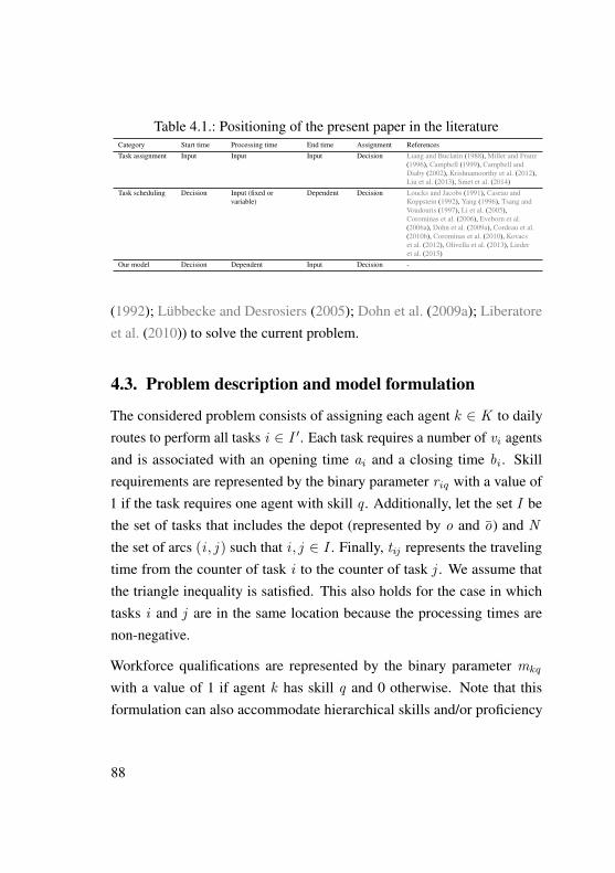
Table 4.1.: Positioning of the present paper in the literatureCategory Start time Processing time End time Assignment ReferencesTask assignment Input Input Input Decision Liang and Buclatin (1988), Miller and Franz

(1996), Campbell (1999), Campbell andDiaby (2002), Krishnamoorthy et al. (2012),Liu et al. (2013), Smet et al. (2014)

Task scheduling Decision Input (fixed orvariable)

Dependent Decision Loucks and Jacobs (1991), Caseau andKoppstein (1992), Yang (1996), Tsang andVoudouris (1997), Li et al. (2005),Corominas et al. (2006), Eveborn et al.(2006a), Dohn et al. (2009a), Cordeau et al.(2010b), Corominas et al. (2010), Kovacset al. (2012), Olivella et al. (2013), Liederet al. (2015)

Our model Decision Dependent Input Decision -

(1992); Lubbecke and Desrosiers (2005); Dohn et al. (2009a); Liberatoreet al. (2010)) to solve the current problem.

4.3. Problem description and model formulation

The considered problem consists of assigning each agent k 2 K to dailyroutes to perform all tasks i 2 I

0. Each task requires a number of vi

agentsand is associated with an opening time a

i

and a closing time b

i

. Skillrequirements are represented by the binary parameter r

iq

with a value of1 if the task requires one agent with skill q . Additionally, let the set I bethe set of tasks that includes the depot (represented by o and o) and N

the set of arcs (i , j ) such that i , j 2 I . Finally, tij

represents the travelingtime from the counter of task i to the counter of task j . We assume thatthe triangle inequality is satisfied. This also holds for the case in whichtasks i and j are in the same location because the processing times arenon-negative.

Workforce qualifications are represented by the binary parameter m

kq

with a value of 1 if agent k has skill q and 0 otherwise. Note that thisformulation can also accommodate hierarchical skills and/or proficiency

88

levels, because only the values of mkq

need to be changed for this purpose.Furthermore, every day, every agent departs and arrives at the depot duringhis/her working shift [e

k

, fk

] (plus overtime).

Six decision variables are used. First, the binary variable x

ijk

assigns asequence of tasks to an agent:

x

ijk

=

8<

:1, if agent k goes directly from task i to task j

0, otherwise.

Note that for agents with no assignments, empty routes (xook

= 1) areallowed.

Second, binary variable y

ik

assigns tasks to agents to simplify the notation:

y

ik

=

8<

:1, if task i is assigned to agent k

0, otherwise.

Third, outsourcing agents is allowed at a cost. The variable outi

representsthe number of outsourced agents for task i , with a maximum value ofout

max

i

.

Fourth, the arrival time of agent k at task i is defined by the positive variables

ik

. Fifth, a task can be processed only after its opening time a

i

, i.e., if anagent arrives earlier, he/she waits at no cost. If an agent starts the task aftera

i

, we penalize the delay using the positive variable w

ik

, defined as

89

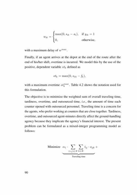
w

ik

=

8<

:max(0, s

ik

� a

i

), if yik

= 1

0, otherwise,

with a maximum delay of wmax .

Finally, if an agent arrives at the depot at the end of the route after theend of his/her shift, overtime is incurred. We model this by the use of thepositive, dependent variable ot

k

defined as

ot

k

= max(0, sok

� f

k

),

with a maximum overtime ot

max

k

. Table 4.2 shows the notation used forthis formulation.

The objective is to minimize the weighted sum of overall traveling time,tardiness, overtime, and outsourced time, i.e., the amount of time eachcounter opened with outsourced personnel. Traveling time is a concern forthe agents, who prefer working at counters that are close together. Tardiness,overtime, and outsourced agent-minutes directly affect the ground-handlingagency because they implicate the agency’s financial interest. The presentproblem can be formulated as a mixed-integer programming model asfollows:

Minimize ↵1 ·X

(i,j )2N

X

k2K

t

ij

· xijk

| {z }Traveling time

+

90

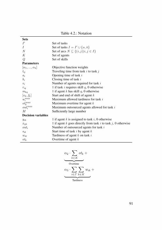
Table 4.2.: NotationSetsI

0 Set of tasksI Set of tasks I = I

0 [ {o, o}N Set of arcs N ✓ {(i , j )|i , j 2 I }K Set of agentsQ Set of skillsParameters[↵1, ...,↵4] Objective function weightst

ij

Traveling time from task i to task j

a

i

Opening time of task i

b

i

Closing time of task i

v

i

Number of agents required for task i

r

iq

1 if task i requires skill q , 0 otherwisem

kq

1 if agent k has skill q , 0 otherwise[e

k

, fk

] Start and end of shift of agent kw

max

i

Maximum allowed tardiness for task i

ot

max

k

Maximum overtime for agent kout

max

i

Maximum outsourced agents allowed for task i

M Sufficiently large numberDecision variablesy

ik

1 if agent k is assigned to task i , 0 otherwisex

ijk

1 if agent k goes directly from task i to task j , 0 otherwiseout

i

Number of outsourced agents for task i

s

ik

Start time of task i by agent kw

ik

Tardiness of agent k on task i

ot

k

Overtime of agent k

↵2 ·X

k2K

ot

k

| {z }Overtime

+

↵3 ·X

i2I

0

X

k2K

w

ik

| {z }Tardiness

+

91

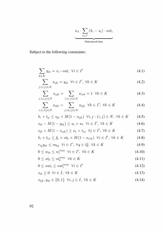
↵4 ·X

i2I

0

(b

i

� a

i

) · outi

| {z }Outsourced time

Subject to the following constraints:

X

k2K

y

ik

= v

i

�out

i

8i 2 I

0 (4.1)

X

j :(i,j )2N

x

ijk

= y

ik

8i 2 I

0, 8k 2 K (4.2)

X

j :(o,j )2N

x

ojk

=

X

i:(i,o)2N

x

iok

= 1 8k 2 K (4.3)

X

i:(i,h)2N

x

ihk

=

X

j :(h,j )2N

x

hjk

8h 2 I

0, 8k 2 K (4.4)

b

i

+ t

ij

s

jk

+M (1� x

ijk

) 8i , j : (i , j ) 2 N , 8k 2 K (4.5)

s

ik

�M (1� y

ik

) a

i

+ w

i

8i 2 I

0, 8k 2 K (4.6)

s

jk

+M (1� x

ojk

) � e

k

+ t

oj

8j 2 I

0, 8k 2 K (4.7)

b

i

+ t

io

f

k

+ ot

k

+M (1� x

iok

) 8i 2 I

0, 8k 2 K (4.8)

r

iq

y

ik

m

kq

8i 2 I

0, 8q 2 Q , 8k 2 K (4.9)

0 w

ik

w

max

i

8i 2 I

0, 8k 2 K (4.10)

0 ot

k

ot

max

k

8k 2 K (4.11)

0 out

i

out

max

i

8i 2 I

0 (4.12)

s

ik

� 0 8i 2 I , 8k 2 K (4.13)

x

ijk

, yik

2 {0, 1} 8i , j 2 I , 8k 2 K (4.14)

92

Constraints (4.1) and (4.2) ensure that the number of required agents (avail-able or outsourced) is assigned to all tasks. Constraint (4.3) ensures thateach agent starts and ends his/her route at the depot. Constraint (4.4)ensures flow conservation when visiting a counter for a task. Constraint(4.5) allows for processing a task only if its preceding task is completed.Constraint (4.6) states that an agent can arrive at a counter only before atask’s opening time, otherwise, tardiness occurs. The routes’ duration limitand overtime are defined by constraints (4.7) and (4.8). Constraint (4.9)ensures that the skill requirements of each task are fulfilled. Constraints(4.10), (4.11), and (4.12) define the bounds for tardiness, overtime, and out-sourced agents, respectively. Finally, constraints (4.13) and (4.14) definethe positive and binary variables, respectively.

4.4. Branch-and-price algorithm

In this section, we present a decomposition of the problem into a masterproblem and subproblems as proposed by Dantzig (1954). This decompo-sition can be then solved by a generic column generation method as theones proposed by Barnhart et al. (1998), Lubbecke and Desrosiers (2005),and Liberatore et al. (2010), among others. The primary idea is to use themaster problem to select agent-schedules from a pool of feasible routesgenerated by the subproblems.

Master Problem Let Pk

be the set of feasible routes containing se-quences of tasks (i.e., paths) for each agent k 2 K , and �

kp

be a binaryvariable equal to 1 only if path p of agent k is used and 0 otherwise. Addi-tionally, let ✓

ikp

be a parameter equal to 1 if task i is in path p of agent k

93

and 0 otherwise. Then, the integer master problem (MP) can be defined asfollows:

MinimizeX

k2K

X

p2P

k

c

kp

�kp

+ ↵4 ·X

i2I

0

out

i

(4.15)

Subject to:

X

k2K

X

p2P

d

✓ip

�kp

= v

i

�out

i

8i 2 I

0 (4.16)

X

p2P

k

�kp

= 1 8k 2 K (4.17)

out

i

out

max

i

8i 2 I

0 (4.18)

�kp

2 {0, 1} 8k 2 K , 8p 2 P

k

(4.19)

Where the cost of a path p 2 P

d

is defined by:

c

kp

=↵1 ·X

(i,j )2N

X

k2K

t

ij

· xijk

+

↵2 ·X

i2I

0

X

k2K

w

ik

+ ↵3 ·X

k2K

ot

k

(4.20)

The objective is to minimize the overall costs (4.15). The set partitioningconstraints (4.16) ensure that demand is satisfied either by available agentsor outsourcing. Convexity constraints (4.17) state that exactly one route isused per agent. Constraint (4.18) ensures that the number of outsourcedagents remains below the maximum allowed. Finally, constraint (4.19)

94

defines the binary requirements for the assignment variables. The linearrelaxation of this formulation (LMP), which is obtained by relaxing con-straint (4.19), can be used to obtain a lower bound on the MP. However, setP

k

may contain a large number of feasible routes, thus making the solutionto this problem computationally intractable. Therefore, in a column genera-tion approach, only subset P 0

k

⇢ P

k

of routes are considered in a restrictedmaster problem (RMP). Additional feasible columns are obtained using theiterative solution of each subproblem, which consists of finding routes foreach agent with negative reduced cost c

kp

:

c

kp

= c

kp

�X

i2I

0

✓ikp

⇡i

� ⇢k

=

X

(i,j )2N

X

k2K

(↵1 · tij � ⇡i

) · xijk

+ ↵2 ·X

i2I

0

X

k2K

w

ik

+ ↵3 ·X

k2K

ot

k

� ⇢k

where ⇡i

, and ⇢k

correspond to the dual values of constraints (4.16) and(4.17) in the optimal solution of the RMP. These values are then passed tothe subproblems from which single-agent routes are obtained.

Pricing Problems We let I 0sub

k

⇢ I

0 and I

sub

k

⇢ I be the set of taskswhich can be processed by agent k . Also let N

sub

k

= {(i , j )|i , j 2 I

sub

k

}.Then, each k�subproblem can be defined as follows:

95

Minimize c

kp

=

X

(i,j )2N

(↵1 · tij � ⇡i

) · xij

+

↵2 ·X

i2I

0

w

i

+ ↵3 · ot � ⇢k

(4.21)

X

j :(i,j )2N

sub

k

x

ij

= y

i

8i 2 I

0sub

k

(4.22)

X

j :(o,j )2N

sub

k

x

oj

=

X

i:(i,o)2N

sub

k

x

io

= 1 (4.23)

X

i:(i,h)2N

sub

k

x

ihk

�X

j :(h,j )2N

sub

k

x

hj

= 0 8h 2 I

0sub

k

(4.24)

b

i

+ t

ij

�M (1� x

ij

) s

j

8i , j : (i , j ) 2 N

sub

k

(4.25)

s

i

�M (1� y

i

) a

i

+ w

i

8i 2 I

0sub

k

(4.26)

s

j

+M (1� x

oj

) � e + t

oj

8j 2 I

0sub

k

(4.27)

b

i

+ t

io

�M (1� x

io

) f + ot 8i 2 I

0sub

k

(4.28)

0 w

i

w

max

i

8i 2 I

0sub

k

(4.29)

0 ot ot

max (4.30)

s

i

� 0 8i 2 I

sub

k

(4.31)

x

ij

, yi

2 {0, 1} 8i , j 2 I

sub

k

(4.32)

where x

ij

is a binary variable with a value of 1 if the arc (i , j ) is used and0 otherwise. s

i

and w

i

are positive variables corresponding to the startingtime and the tardiness of task i , whereas ot is a positive variable that

96

represents the overtime of the route. The objective is to find a route with aminimum reduced cost (4.21). Constraint (4.22) initializes the variable y

i

.Constraints (4.23) and (4.24) ensure the feasibility of the route. Constraint(4.25) defines the task’s starting time, whereas constraint (4.26) ensuresthat a counter’s opening time is respected; otherwise, the agent is tardy.Constraints (4.27) and (4.28) define shift-length limits, and if an agentarrives at the depot after closing time, overtime is incurred. Constraints(4.29) and (4.30) define the bounds for the tardiness and overtime variables,respectively. Finally, positive variable (4.31) and binary variable (4.32) aredefined.

These subproblems correspond to an Elementary Shortest Path Problemwith Resource Constraints (ESPPRC). The requirement of elementary paths(i.e., paths that visit each task no more than once) is required because thereduced cost associated with each task may lead to negative cost cycles.Note that ESPPRC in graphs with negative cost cycles is strongly NP-hard(Dror, 1994). This represents a major drawback because in our algorithm,we need to solve these subproblems several times. Therefore, an efficientsolution approach is required.

4.4.1. Labeling algorithm

Because the ESPPRC can be computationally expensive to solve, a typicalapproach is to relax the elementariness requirement and then to solve it as aShortest Path Problem with Resource Constraints (SPPRC) (i.e., subcyclesare allowed). The SPPRC can be solved using dynamic programming,which can be solved in pseudo-polynomial time (Desrochers et al., 1992).Nevertheless, the main drawback to this approach is that it weakens the

97

lower bound computed by the column generation phase (Bode and Irnich,2014a). Conversely, dynamic programming can be used to solve the ESP-PRC (Feillet et al., 2004; Liberatore et al., 2010) to provide better lowerbounds, albeit with a higher computational cost. It is possible, however, tosolve the pricing problem described in the previous section as an SPPRCwhile ensuring elementary paths by exploiting the problem structure.

Below, we describe a dynamic programming algorithm we propose for thesolution of the pricing problems of our branch-and-price approach, alongwith details on its implementation. Similar algorithms are proposed byFeillet et al. (2004) and Liberatore et al. (2010) also to solve the pricingproblems embedded in a column generation algorithm to solve the classicalVehicle Routing Problem with Time Windows (VRPTW). Mainly, ouralgorithm differs from theirs on the fact that end times of the tasks are fixed(thus the processing time of the tasks are start time-dependent) and thatelementary paths are not explicitly required.

In short, the algorithm’s objective is to obtain routes from o to o for anagent such that the reduced cost is minimized. For this purpose, we definethe following concepts. A state associated with task i corresponds to apartial path of visited counters from the depot to i . Each task can beassociated with more than one state because multiple feasible paths can endin the respective task. To represent such states, we use multidimensionalresource vectors or labels represented by L

i

= (i ,Ti

,C (T

i

)), where i isthe last visited task, T

i

is the starting time of task i , and C (T

i

) is the time-dependent cost. Additionally, let U

i

and Pi

represent the set of unprocessedand processed labels for task i , respectively.

The process is initialized by setting sets Ui

and Pi

to the empty set, creatingthe first label L

o

= (o,To

= e,C (T

o

) = 0), and appending L

o

to the

98

unprocessed set. Through the algorithm, labels are extended to successivefeasible labels of the form L

j

= (j ,Tj

,C 0(T

j

)) by appending an addi-tional arc (i , j ) to the partial path o � i and updating its correspondingresources using the following resource extension functions (REF):

T

j

= max(a

j

, bi

+ t

ij

) (4.33)

C

0j

=

8<

:C (T

i

) + c

ij

+max(0,↵2 · (Tj

� a

j

))� ⇡i

, if j 6= o

C (T

i

) + c

ij

+max(0,↵3 · (Tj

� f ))� ⇡i

, if j = o

(4.34)

We note that, in contrast to Feillet et al. (2004) and Liberatore et al. (2010),this algorithm takes into consideration the closing time of a counter b

i

instead of recursively calculating T

j

from previous states. In this way,the characteristic of fixed ending times from our problem is consideredin our algorithm. Then, iteratively, the labels with the minimum timeare selected from the unprocessed set to search for possible extensionsalong their arcs. These extensions can only be made on feasible labels.A label (i ,T

i

,C (T

i

)) is feasible if Ti

b

i

+ w

max |i 6= o and T

i

b

i

+ ot

max |i = o. Labels that do not satisfy these conditions are discarded.If feasible, the new extended labels are added to the unprocessed set andthe currently explored labels are added to the processed set.

Because dual information may produce arcs with negative costs, sub-cyclesare not strictly forbidden. Using additional vectors on each label, as pro-posed by Feillet et al. (2004) and Liberatore et al. (2010), the elementarinessof the paths can be enforced. However, from the time extension function(4.33) we can observe that the time consumption is strictly positive, asT

j

�T

i

� 0 for all (i , j ) 2 N

sub

k

if such extension is feasible. Because the

99

algorithm chooses the label with the least time consumption from the set ofunprocessed labels, it is then guaranteed that all feasible extensions from agiven label have a non-decreasing consumption of the time resource (Irnichet al., 2005), effectively forbidding sub-cycles because of the definitionof feasibility. In this way, our algorithm mimics an acyclic graph withoutthe need to explicitly enforce elementariness at the label-extension step.Therefore, in contrast to Feillet et al. (2004) and Liberatore et al. (2010),in the proposed algorithm no elementariness check is conducted whileextending the labels.

To keep the size of these sets tractable, dominance rules are requiredto discard (multiple) labels that cannot lead to an optimal solution. Forthis purpose, dominance rules are applied. Let L

i

= (i ,Ti

,C (T

i

)) andL

0i

= (i ,T 0i

,C 0(T

0i

)) be two labels of task i . Then, Li

dominates L

0i

ifL

i

< L

0i

component-wise, i.e., if Ti

T

0i

, C (T

i

) C

0(T

0i

), and atleast one of the inequalities is strict. If a label is dominated, then it can bediscarded; when all components are equal, both labels are retained.

Once all paths arriving at the depot o are obtained and no unprocessedlabels remain, the label with the minimum cost is selected and correspondsto the optimal solution of the respective subproblem. Its correspondingreduced cost is determined by ¯c

kp

= C (T

o

)� ⇢k

. If more than one labelhas the same cost, and none can be dominated, then all of them are addedas columns of the reduced master problem. Algorithm 3 shows an overviewof the labeling process.

100

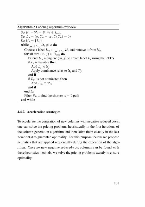
Algorithm 3 Labeling algorithm overviewSet U

i

= Pi

= ? 8i 2 I

sub

k

Set Lo

= (o,To

= e

k

,C (T

o

) = 0)

Set Uo

= {Lo

}while

Si2I

sub

k

Ui

6= ? doChoose a label L

m

2S

i2I

sub

Ui

and remove it from Um

for all arcs (m, j ) 2 N

sub

doExtend L

m

along arc (m, j ) to create label Lj

using the REF’sif L

j

is feasible thenAdd L

j

to Uj

Apply dominance rules to Uj

and Pj

end ifif L

m

is not dominated thenAdd L

m

to Pm

end ifend forFilter P

o

to find the shortest o � o pathend while

4.4.2. Acceleration strategies

To accelerate the generation of new columns with negative reduced costs,one can solve the pricing problems heuristically in the first iterations ofthe column generation algorithm and then solve them exactly in the lastiteration(s) to guarantee optimality. For this purpose, below we proposeheuristics that are applied sequentially during the execution of the algo-rithm. Once no new negative reduced-cost columns can be found withthese heuristics methods, we solve the pricing problems exactly to ensureoptimality.

101

Initialization To provide the initial columns for the column-generationprocedure, we use two approaches. First, we sort the agents by increasingshift length and for each agent, we run the labeling algorithm, stoppingwhen a preset number of shortest paths are found. Each path is theninserted as a column of the reduced master problem (RMP). Second, weuse a modified version of the insertion heuristic from Solomon (1987).This algorithm can be summarized as follows: (i) for each agent k 2 K ,we sequentially initialize routes by choosing the task with the highestprocessing time; (ii) for each task h available to team k , we calculate theoperation costs obtained from inserting it, if feasible, into each arc (i , j )

of the initial route; (iii) the insertion (i , h, j )⇤ with the minimum cost isselected and the initial route is updated accordingly at that point, steps (ii)and (iii) are repeated until no further tasks can be inserted; (iv) the resultingroutes are inserted as columns of (RMP). If a task is not included in anypath from the two methods, then it is included in the RMP as an artificialcolumn with a high cost.

(H1) Partial pricing Each k subproblem focuses on the route of a spe-cific agent and thus, only the tasks corresponding to this subproblem areconsidered. Depending on the task’s characteristics, it is possible for multi-ple agents to be assigned to them with the same route cost. In terms of thecolumn-generation procedure, this means that the marginal values ⇢

k

havezero values, i.e., there is no prize to earn for dispatching agent k . We canexploit this fact to reduce the number of subproblems in each iteration bysolving only those subproblems with marginal values different from zero.If no subproblem satisfies this condition, we solve all of the subproblems

102

until three columns with reduced cost are found, and the column-generationphase continues.

(H2) Relaxed dominance rules One way to accelerate the solution of thesubproblems is to relax the dominance rules from the exact labeling algo-rithm. This is done by testing the dominance of only a subset of the labels’resources: for two labels L

i

= (i ,Ti

,C (T

i

)) and L

0i

= (i ,T 0i

,C 0(T

0i

)),L

i

dominates L0i

if C (T

i

) C

0(T

0i

).

(H3) Partial pricing and partial dominance rules This approach con-sists of a combination of both of the previously described heuristics: H1 andH2. Therefore, partial pricing is applied in the column-generation phaseand relaxed dominance rules are used in the solution to the subproblems.

4.4.3. General procedure

In this section, we outline the proposed branch-and-price algorithm, whichprimarily consists of a column-generation algorithm embedded in a branch-and-bound procedure to guarantee integrality. Additionally, further detailson the implementation of the column-generation algorithm, data prepro-cessing, search strategies, and branching rules are presented.

Column generation The column-generation process can be describedas follows. The algorithm is initialized by the insertion heuristic. Themaster problem is solved using a set of artificial columns obtained by theintroduction of slack variables with a high cost to ensure primal feasibility.Because of their high cost, these variables eventually leave the basis, once

103

further feasible columns are obtained. From the solution to the masterproblem, the marginal values are obtained and passed to the subproblems.New routes (i.e., columns) are obtained by solving the subproblems. Ifcolumns are found with a negative reduced cost, the column-generationprocess is started again. Otherwise, an optimal solution for the reducedmaster problem (and thus, for the master problem) is found. If this solutionis an integer, then it is an optimal solution to the original problem; if not,then it corresponds to a valid fractional lower bound. Next, branching onfractional variables is required and column generation is applied on eachnode with its respective fractional bounds.

Preprocessing Each subproblem k focuses on a subset Isub

k

⇢ I of tasksbecause of the skill requirements. It is possible to further reduce this subsetby removing tasks that cannot be operated by k agents based on the shiftstarting and ending times and the overtime limit otmax

k

. Additionally, onecan reduce the number of arcs considered in the subproblem’s set N

sub

k

by redefining it as N

sub

k

= {(i , j )|i , j 2 I

sub

k

, bi

+ (b

i

� a

i

) + t

i,j b[j ] + w

max

i

}. This means that infeasible arcs caused by a violation of themaximum tardiness bound are eliminated.

Branching We explore the branching tree using a depth-first strategy.In this way, the solution from the parent node is used as a warm start forthe children nodes (eliminating the columns that do not comply with theirrespective branching bounds).

One common branching rule is to branch on the arcs (i , j ), because thisrule is simple to incorporate into the subproblems by removing arcs inN

sub

k

, and deleting the columns that violate the branching rule. However,

104

this approach does not provide strong integrality bounds for our problem,because tasks i and j might require the assignment of more than one agent.Therefore, we use the following branching rule: for each node on thebranching tree, we define the set A as the set of fractional assignments(i , k) such that 0 <

ik

< 1, where ik

=

Pp2P

k

✓ikp

�kp

; ✓ikp

is equalto 1 if task j is assigned to agent k ’s path p, and 0 otherwise. Then, theassignment (i , k)⇤ is selected as follows:

(i , k)⇤ 2 argmax

(i,k)2A{(b

i

� a

i

) ·min( ik

, 1� ik

)}

From this node, two successors are generated:

• A left node with ik

= 0, where agent k cannot be assigned to taski , i.e., this task is removed from its respective subproblem’s graphand columns using this assignment are discarded.

• A right node with ik

= 1, where this arc is fixed, i.e., agent k isassigned to task i .

Upper bound update After exploring a given number of nodes, it is pos-sible to obtain new information on the development of the (integer) upperbound by solving the reduced master problem (RMP) of the incumbentnode as an integer program. If the new bound is better than the best boundfound so far, then the bound is updated and nodes with a more expensivesolution are pruned. There is, however, a trade-off related to computationtime, because too often, solving the integer RMP can be computationallyexpensive and not necessarily beneficial to the quality of the upper bound.

105

4.5. Numerical Experiments

For our numerical tests, we use real-world input data from a Germanground-handling agency to test the performance of our proposed algorithm.First, in Section 4.5.1, we use the provided data to test the performanceof the branch-and-price algorithm. We also evaluate the gains in com-putation times obtained by solving the pricing problems using shortestpaths instead of elementary shortest paths in the column-generation phaseof our algorithm. Second, in Section 4.5.2, we generate instances withdifferent shift lengths to evaluate the performance of our algorithm underdifferent shift profiles. Third, we generate instances of larger size basedon the existing information in Section 4.5.3 to test the performance of oursolution approaches in larger settings. Fourth, in Section 4.5.4, we conducta sensitivity analysis to evaluate the impact of the maximum tardiness inthe resulting schedules. All of the methods are implemented in Python2.7.3 using the Gurobi 5.6 solver on a 2.9 GHz Intel Core i7 machine with8 GB of RAM in OS X Yosemite 10.10.14.

4.5.1. Performance tests

The data consist of 24 real-world instances, corresponding to flight sched-ules on different days. In addition, we include 4 realistic but not real in-stances included in Appendix A and also available at http://stolletz.bwl.uni-mannheim.de/en/library.

Table 4.3 presents information regarding the tasks and the workforce foreach instance: the number of tasks, the minimum, maximum, and averageoccupation time (in minutes), the average agent requirements, and thenumber of tasks requiring each skill is shown. Also, this table presents the

106

number of agents, the minimum, maximum, and average shift length (inminutes), as well as the number of agents qualified on each skill, for eachinstance. The location of the check-in counters is known, and the travelingdistance between the locations is provided by the ground-handling agency.Based on the contracts with the airlines, the maximum tardiness is set to one-half of the duration of each task (wmax

ik

= 0.5 ·(bi

� a

i

) 8i 2 I , 8k 2 K ),and the maximum outsourcing is set such that at least one normal agent ispresent at each task (outmax

i

= v

i

� 1 8i 2 I ). For each instance, a shiftplan is also provided that includes information about the qualifications, shiftstart, and shift end for each agent. The shift length per agent has a value ofbetween 3 and 10 hours, and each agent can be qualified in one or moreof the 12 available skills. To comply with labor regulations, the maximumovertime per agent is set such that the shift length plus overtime cannotexceed 10 hours. Finally, based on observations from the ground-handlingagency’s management, the weights for the objective function are set as[↵1,↵2,↵3,↵4] = [0.1, 0.2, 0.3, 0.4].

The results for all of the test instances are obtained from the solution of theMIP formulation and two versions of the branch-and-price algorithm: oneon which the subproblems are modeled as shortest path problems (SPPRC)and the other on which the subproblems are modeled as elementary short-est path problems (ESPPRC). The solutions reported are those obtainedwithin a time limit of 1 hour. We use the exact solutions from the BP tocalculate ex-post the absolute gap of the MIP results for the cases whereoptimality is not proven within the time limit. For the MIP results, Table4.4 presents the objective function value, the computation time (in minutes),and the absolute gap to optimality (in percentage). For both versions ofthe branch-and-price (BP) results, the table shows the objective function

107

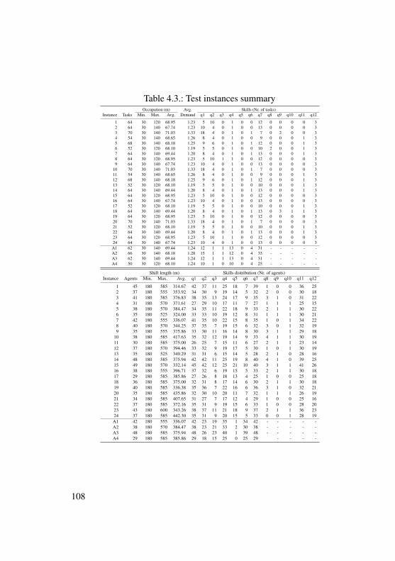
Table 4.3.: Test instances summaryOccupation (m) Avg. Skills (Nr. of tasks)

Instance Tasks Min. Max. Avg. Demand q1 q2 q3 q4 q5 q6 q7 q8 q9 q10 q11 q12

1 64 30 120 68.95 1.23 5 10 0 1 0 0 12 0 0 0 0 32 64 30 140 67.74 1.23 10 4 0 1 0 0 13 0 0 0 0 33 70 30 140 71.03 1.33 18 4 0 1 0 1 7 0 2 0 0 34 54 30 140 68.65 1.26 8 4 0 1 0 0 9 0 0 0 1 35 68 30 140 68.18 1.25 9 6 0 1 0 1 12 0 0 0 1 36 52 30 120 68.10 1.19 5 5 0 1 0 0 10 2 0 0 1 37 64 30 140 69.44 1.20 8 4 0 1 0 1 13 0 0 0 1 38 64 30 120 68.95 1.23 5 10 1 1 0 0 12 0 0 0 0 39 64 30 140 67.74 1.23 10 4 0 1 0 0 13 0 0 0 0 3

10 70 30 140 71.03 1.33 18 4 0 1 0 1 7 0 0 0 0 311 54 30 140 68.65 1.26 8 4 0 1 0 0 9 0 0 0 1 312 68 30 140 68.18 1.25 9 6 0 1 0 1 12 0 0 0 1 313 52 30 120 68.10 1.19 5 5 0 1 0 0 10 0 0 0 1 314 64 30 140 69.44 1.20 8 4 0 1 0 1 13 0 0 0 1 315 64 30 120 68.95 1.23 5 10 0 1 0 0 12 0 0 0 0 316 64 30 140 67.74 1.23 10 4 0 1 0 0 13 0 0 0 0 317 52 30 120 68.10 1.19 5 5 0 1 0 0 10 0 0 0 1 318 64 30 140 69.44 1.20 8 4 0 1 0 1 13 0 3 1 1 319 64 30 120 68.95 1.23 5 10 0 1 0 0 12 0 0 0 0 320 70 30 140 71.03 1.33 18 4 0 1 0 1 7 0 0 0 0 321 52 30 120 68.10 1.19 5 5 0 1 0 0 10 0 0 0 1 322 64 30 140 69.44 1.20 8 4 0 1 0 1 13 0 0 0 1 323 64 30 120 68.95 1.23 5 10 1 1 0 0 12 0 0 0 0 324 64 30 140 67.74 1.23 10 4 0 1 0 0 13 0 0 0 0 3A1 62 30 140 69.44 1.24 12 1 1 13 0 4 31 - - - - -A2 66 30 140 68.18 1.28 15 1 1 12 0 4 33 - - - - -A3 62 30 140 69.44 1.24 12 1 1 13 0 4 31 - - - - -A4 50 30 120 68.10 1.24 10 1 0 10 0 4 25 - - - - -

Shift length (m) Skills distribution (Nr. of agents)Instance Agents Min. Max. Avg. q1 q2 q3 q4 q5 q6 q7 q8 q9 q10 q11 q12

1 45 180 585 314.67 42 37 11 25 18 7 39 1 0 0 36 252 37 180 555 353.92 34 30 9 19 14 5 32 2 0 0 30 183 41 180 585 376.83 38 35 13 24 17 9 35 3 1 0 31 224 31 180 570 371.61 27 29 10 17 11 7 27 1 1 1 25 155 38 180 570 384.47 34 35 11 22 18 9 33 2 1 1 30 226 35 180 525 324.00 33 33 10 19 12 8 31 1 1 1 30 217 42 180 555 336.07 41 35 10 22 15 8 35 1 0 1 34 228 40 180 570 344.25 37 35 7 19 15 6 32 3 0 1 32 199 35 180 555 375.86 33 30 11 16 14 8 30 3 1 1 29 18

10 38 180 585 417.63 35 32 12 19 14 9 33 4 1 1 30 1911 30 180 585 375.00 26 25 7 15 11 6 27 2 1 1 23 1412 37 180 570 394.46 33 32 9 19 17 5 30 1 0 1 30 1913 35 180 525 349.29 31 31 6 15 14 5 28 2 1 0 28 1614 48 180 585 375.94 42 42 11 25 19 8 40 4 1 0 39 2515 49 180 570 332.14 45 42 12 25 21 10 40 3 1 1 41 2616 38 180 555 396.71 37 32 6 19 15 5 33 2 1 1 30 1817 29 180 585 385.86 27 26 8 18 13 4 25 1 0 0 25 1818 36 180 585 375.00 32 31 8 17 14 6 30 2 1 1 30 1819 40 180 585 336.38 35 36 7 22 16 6 36 3 1 0 32 2120 35 180 585 435.86 32 30 10 20 11 7 32 1 1 1 26 1921 34 180 585 407.65 31 27 7 17 12 4 29 1 0 0 25 1622 37 180 585 372.16 35 31 9 19 15 6 33 1 0 0 28 2023 43 180 600 343.26 38 37 11 21 18 9 37 2 1 1 36 2324 37 180 585 442.30 35 31 9 20 15 5 33 0 0 1 28 19A1 42 180 555 336.07 42 23 19 35 1 34 42 - - - - -A2 38 180 570 384.47 38 23 21 33 2 30 38 - - - - -A3 48 180 585 375.94 48 26 23 40 1 39 48 - - - - -A4 29 180 585 385.86 29 18 15 25 0 25 29 - - - -

108

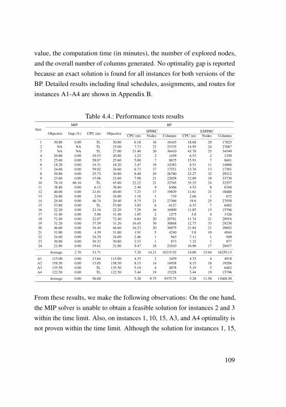
value, the computation time (in minutes), the number of explored nodes,and the overall number of columns generated. No optimality gap is reportedbecause an exact solution is found for all instances for both versions of theBP. Detailed results including final schedules, assignments, and routes forinstances A1-A4 are shown in Appendix B.

Table 4.4.: Performance tests results

Inst.MIP BP

Objective Gap (%) CPU (m) Objective SPPRC ESPPRCCPU (m) Nodes Columns CPU (m) Nodes Columns

1 30.80 0.00 TL 30.80 6.18 16 16445 18.68 20 178252 NA NA TL 25.00 7.73 22 25335 14.95 24 276873 NA NA TL 27.00 21.40 20 36410 45.78 25 345494 20.80 0.00 10.53 20.80 1.23 2 1439 6.53 2 13505 25.60 0.00 58.87 25.60 5.00 7 8675 15.93 7 84016 18.20 0.00 14.31 18.20 3.47 19 14383 8.51 11 148887 24.60 0.00 59.02 24.60 6.73 17 17551 13.76 13 173018 30.80 0.00 25.73 30.80 8.40 29 26780 23.27 32 292129 23.60 0.00 15.06 23.60 7.98 21 22658 12.89 18 23730

10 76.10 66.16 TL 45.80 22.22 21 32765 35.25 24 3255711 38.80 0.00 6.15 38.80 2.40 9 6566 4.53 8 676012 40.00 0.00 21.81 40.00 7.23 17 19029 11.61 21 1848013 24.80 0.00 2.54 24.80 1.10 1 719 2.66 1 67214 29.40 0.00 46.74 29.40 9.75 21 27366 19.6 25 2703815 53.80 0.00 TL 53.80 3.85 6 6127 6.35 7 648216 22.20 0.00 21.16 22.20 7.29 16 16909 11.85 15 1579617 31.40 0.00 5.86 31.40 1.05 2 1275 3.8 4 132618 72.40 0.00 22.67 72.40 6.84 20 20761 11.74 21 2091619 31.20 0.00 37.59 31.20 10.45 30 30848 12.73 33 2923020 46.60 0.00 34.44 46.60 16.23 20 30075 21.84 21 2969221 31.80 0.00 4.39 31.80 1.91 5 4240 3.8 10 404422 24.60 0.00 24.29 24.60 2.46 1 943 7.11 1 94923 30.80 0.00 30.32 30.80 2.53 1 873 7.32 1 87724 21.80 0.00 19.61 21.80 9.47 18 21010 16.96 17 20457

Average 2.76 31.71 7.20 14.21 16215.92 14.06 15.04 16259.13

A1 115.00 0.00 13.64 115.00 4.33 2 2459 4.33 4 4918A2 158.50 0.00 13.05 158.50 8.15 14 14938 8.15 18 19206A3 135.50 0.00 TL 135.50 5.19 4 4878 5.19 5 6482A4 122.50 0.00 TL 122.50 3.44 19 15228 3.44 19 15796

Average 0.00 56.68 5.28 9.75 9375.75 5.28 11.50 11600.50

From these results, we make the following observations: On the one hand,the MIP solver is unable to obtain a feasible solution for instances 2 and 3within the time limit. Also, on instances 1, 10, 15, A3, and A4 optimality isnot proven within the time limit. Although the solution for instances 1, 15,

109

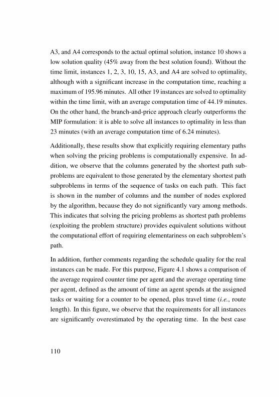
A3, and A4 corresponds to the actual optimal solution, instance 10 shows alow solution quality (45% away from the best solution found). Without thetime limit, instances 1, 2, 3, 10, 15, A3, and A4 are solved to optimality,although with a significant increase in the computation time, reaching amaximum of 195.96 minutes. All other 19 instances are solved to optimalitywithin the time limit, with an average computation time of 44.19 minutes.On the other hand, the branch-and-price approach clearly outperforms theMIP formulation: it is able to solve all instances to optimality in less than23 minutes (with an average computation time of 6.24 minutes).

Additionally, these results show that explicitly requiring elementary pathswhen solving the pricing problems is computationally expensive. In ad-dition, we observe that the columns generated by the shortest path sub-problems are equivalent to those generated by the elementary shortest pathsubproblems in terms of the sequence of tasks on each path. This factis shown in the number of columns and the number of nodes exploredby the algorithm, because they do not significantly vary among methods.This indicates that solving the pricing problems as shortest path problems(exploiting the problem structure) provides equivalent solutions withoutthe computational effort of requiring elementariness on each subproblem’spath.

In addition, further comments regarding the schedule quality for the realinstances can be made. For this purpose, Figure 4.1 shows a comparison ofthe average required counter time per agent and the average operating timeper agent, defined as the amount of time an agent spends at the assignedtasks or waiting for a counter to be opened, plus travel time (i.e., routelength). In this figure, we observe that the requirements for all instancesare significantly overestimated by the operating time. In the best case

110

(instance 6), 80% of the operating time is destined to serving tasks, whereasin the worst case (instance 20), this value is only 49%. Overall, in thecurrent schedules, agents spend an average of 60% of their operating timein check-in tasks, 4.5% traveling between counters, and the remainingtime they idle. This effect, however, is a product of the relation betweenflight schedules (e.g., long gaps between flights), shift plans (e.g., longshifts covering periods with no flights), and employee qualifications (e.g.,employees with single qualifications) for which no specific behavior couldbe observed in the tested instances.

Figure 4.1.: Average operating time per agent

Instance

Min

utes

050

100

150

200

250

1 2 3 4 5 6 7 8 9 10 11 12 13 14 15 16 17 18 19 20 21 22 23 24

Avg. requirements

Avg. operatingtime

4.5.2. Impact of shift length

For the following tests, we concentrate on the shift length’s impact on theresulting schedules. For this purpose, we artificially create different shiftplans for each real-world test instance by multiplying the shift length for

111

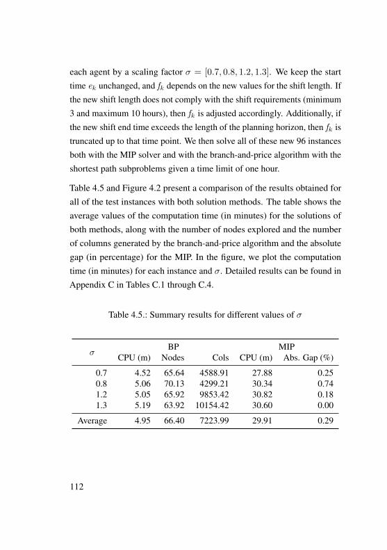
each agent by a scaling factor � = [0.7, 0.8, 1.2, 1.3]. We keep the starttime e

k

unchanged, and f

k

depends on the new values for the shift length. Ifthe new shift length does not comply with the shift requirements (minimum3 and maximum 10 hours), then f

k

is adjusted accordingly. Additionally, ifthe new shift end time exceeds the length of the planning horizon, then f

k

istruncated up to that time point. We then solve all of these new 96 instancesboth with the MIP solver and with the branch-and-price algorithm with theshortest path subproblems given a time limit of one hour.

Table 4.5 and Figure 4.2 present a comparison of the results obtained forall of the test instances with both solution methods. The table shows theaverage values of the computation time (in minutes) for the solutions ofboth methods, along with the number of nodes explored and the numberof columns generated by the branch-and-price algorithm and the absolutegap (in percentage) for the MIP. In the figure, we plot the computationtime (in minutes) for each instance and �. Detailed results can be found inAppendix C in Tables C.1 through C.4.

Table 4.5.: Summary results for different values of �

�BP MIP

CPU (m) Nodes Cols CPU (m) Abs. Gap (%)

0.7 4.52 65.64 4588.91 27.88 0.250.8 5.06 70.13 4299.21 30.34 0.741.2 5.05 65.92 9853.42 30.82 0.181.3 5.19 63.92 10154.42 30.60 0.00

Average 4.95 66.40 7223.99 29.91 0.29

112

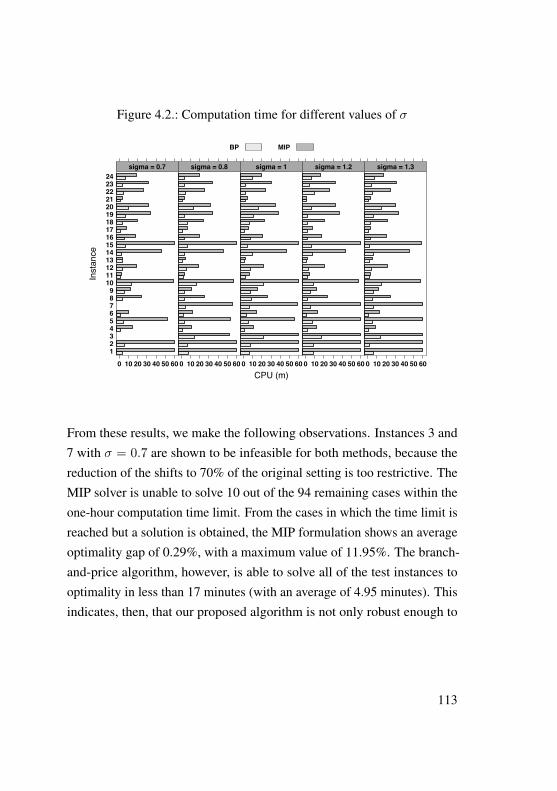
Figure 4.2.: Computation time for different values of �

CPU (m)

Inst

ance

123456789

101112131415161718192021222324

0 10 20 30 40 50 60

sigma = 0.7

0 10 20 30 40 50 60

sigma = 0.8

0 10 20 30 40 50 60

sigma = 1

0 10 20 30 40 50 60

sigma = 1.2

0 10 20 30 40 50 60

sigma = 1.3

BP MIP

From these results, we make the following observations. Instances 3 and7 with � = 0.7 are shown to be infeasible for both methods, because thereduction of the shifts to 70% of the original setting is too restrictive. TheMIP solver is unable to solve 10 out of the 94 remaining cases within theone-hour computation time limit. From the cases in which the time limit isreached but a solution is obtained, the MIP formulation shows an averageoptimality gap of 0.29%, with a maximum value of 11.95%. The branch-and-price algorithm, however, is able to solve all of the test instances tooptimality in less than 17 minutes (with an average of 4.95 minutes). Thisindicates, then, that our proposed algorithm is not only robust enough to

113

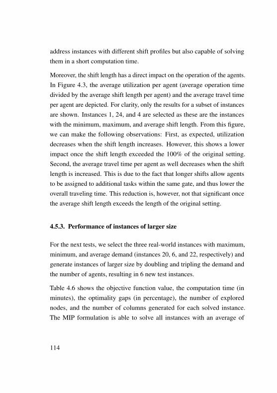
address instances with different shift profiles but also capable of solvingthem in a short computation time.

Moreover, the shift length has a direct impact on the operation of the agents.In Figure 4.3, the average utilization per agent (average operation timedivided by the average shift length per agent) and the average travel timeper agent are depicted. For clarity, only the results for a subset of instancesare shown. Instances 1, 24, and 4 are selected as these are the instanceswith the minimum, maximum, and average shift length. From this figure,we can make the following observations: First, as expected, utilizationdecreases when the shift length increases. However, this shows a lowerimpact once the shift length exceeded the 100% of the original setting.Second, the average travel time per agent as well decreases when the shiftlength is increased. This is due to the fact that longer shifts allow agentsto be assigned to additional tasks within the same gate, and thus lower theoverall traveling time. This reduction is, however, not that significant oncethe average shift length exceeds the length of the original setting.

4.5.3. Performance of instances of larger size

For the next tests, we select the three real-world instances with maximum,minimum, and average demand (instances 20, 6, and 22, respectively) andgenerate instances of larger size by doubling and tripling the demand andthe number of agents, resulting in 6 new test instances.

Table 4.6 shows the objective function value, the computation time (inminutes), the optimality gaps (in percentage), the number of explorednodes, and the number of columns generated for each solved instance.The MIP formulation is able to solve all instances with an average of

114

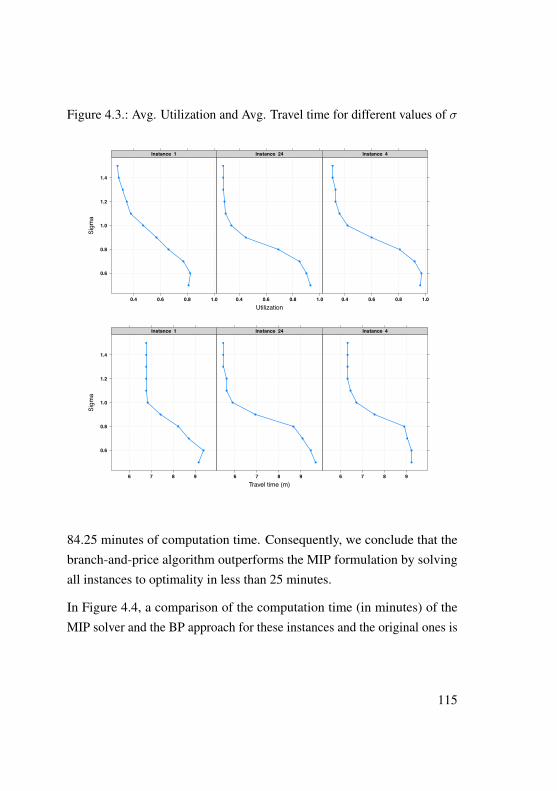
Figure 4.3.: Avg. Utilization and Avg. Travel time for different values of �

Utilization

Sigm

a

0.6

0.8

1.0

1.2

1.4

0.4 0.6 0.8 1.0

Instance 1

0.4 0.6 0.8 1.0

Instance 24

0.4 0.6 0.8 1.0

Instance 4

Travel time (m)

Sigm

a

0.6

0.8

1.0

1.2

1.4

6 7 8 9

Instance 1

6 7 8 9

Instance 24

6 7 8 9

Instance 4

84.25 minutes of computation time. Consequently, we conclude that thebranch-and-price algorithm outperforms the MIP formulation by solvingall instances to optimality in less than 25 minutes.

In Figure 4.4, a comparison of the computation time (in minutes) of theMIP solver and the BP approach for these instances and the original ones is

115

Table 4.6.: Results for large size instances

Instance MIP BPObjective CPU (m) Abs. gap (%) Objective CPU (m) Nodes Columns

6x2 36.40 11.91 0.00 36.40 3.02 5 61836x3 54.40 58.20 0.00 54.40 10.71 13 22983

20x2 93.20 87.09 0.00 93.20 24.27 11 3003020x3 140.40 236.00 0.42 139.80 19.17 4 658222x2 49.20 34.93 0.00 49.20 9.95 6 932422x3 73.80 77.35 0.00 73.80 9.92 18 25373

Average 74.57 84.25 0.07 74.47 12.84 9.50 16745.83

shown. We first note that the computation time increases when increasingthe size of the instances. This was the case for all instances with theexception of instance 6x2 as the BP approach is 2.4 minutes faster than theoriginal instance. Second, we observe that increasing the instance size hasa different impact on both methods on all instances. More specifically, theBP approach shows a lower increase in computation time in comparison tothe MIP solver. This can be explained by the more-efficient exploration ofbranching nodes of the BP approach, as the pricing problems are solved witha pseudo-polynomial algorithm less sensitive to increases in the solutionspace.

4.5.4. Impact of tardiness limit

The final tests focus on the impact of the maximum tardiness limit in thedaily schedules of our planning problem. For this purpose, we selected thereal-world instance that shows the maximum overall tardiness from Section4.5.1 (i.e., instance 15) and modified the original maximum tardiness bound(wmax

i

). In the original setting, this bound corresponds to half of the

116

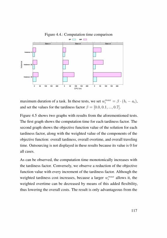
Figure 4.4.: Computation time comparison

CPU (m)

Inst

ance

Instance 20

Instance 22

Instance 6

0 50 100 150 200

Size x 1

0 50 100 150 200

Size x 2

0 50 100 150 200

Size x 3

BP MIP

maximum duration of a task. In these tests, we set wmax

i

= � · (bi

� a

i

),and set the values for the tardiness factor � = [0.0, 0.1, ..., 0.7].

Figure 4.5 shows two graphs with results from the aforementioned tests.The first graph shows the computation time for each tardiness factor. Thesecond graph shows the objective function value of the solution for eachtardiness factor, along with the weighted value of the components of theobjective function: overall tardiness, overall overtime, and overall travelingtime. Outsourcing is not displayed in these results because its value is 0 forall cases.

As can be observed, the computation time monotonically increases withthe tardiness factor. Conversely, we observe a reduction of the objectivefunction value with every increment of the tardiness factor. Although theweighted tardiness cost increases, because a larger wmax

i

allows it, theweighted overtime can be decreased by means of this added flexibility,thus lowering the overall costs. The result is only advantageous from the

117

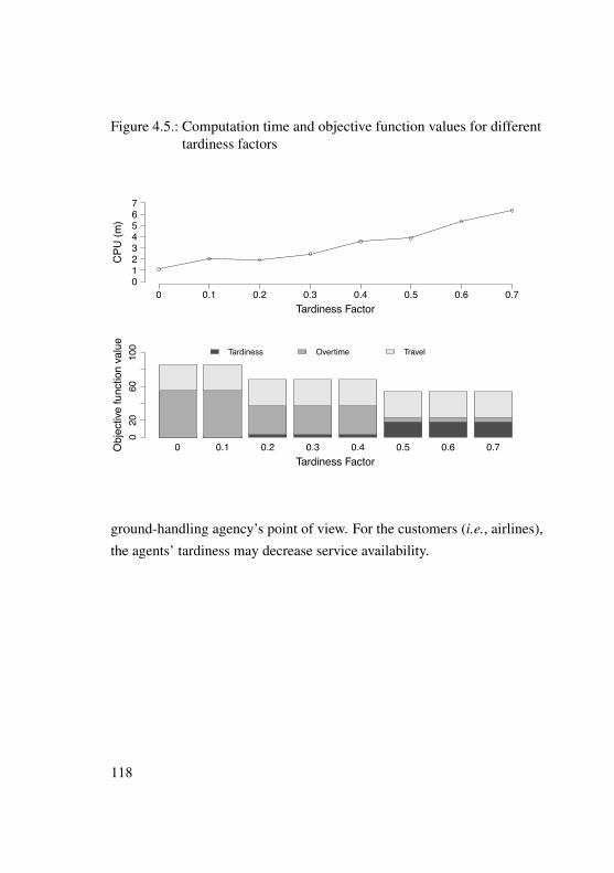
Figure 4.5.: Computation time and objective function values for differenttardiness factors

Tardiness Factor

CPU

(m)

0 0.1 0.2 0.3 0.4 0.5 0.6 0.701234567

0 0.1 0.2 0.3 0.4 0.5 0.6 0.7Tardiness Factor

Obj

ectiv

e fu

nctio

n va

lue

020

6010

0 Tardiness Overtime Travel

ground-handling agency’s point of view. For the customers (i.e., airlines),the agents’ tardiness may decrease service availability.

118

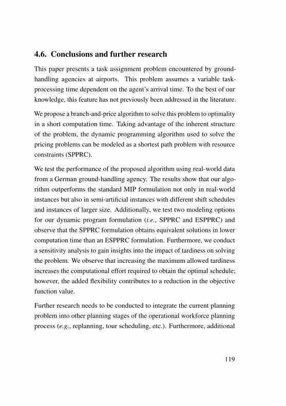
4.6. Conclusions and further research

This paper presents a task assignment problem encountered by ground-handling agencies at airports. This problem assumes a variable task-processing time dependent on the agent’s arrival time. To the best of ourknowledge, this feature has not previously been addressed in the literature.

We propose a branch-and-price algorithm to solve this problem to optimalityin a short computation time. Taking advantage of the inherent structureof the problem, the dynamic programming algorithm used to solve thepricing problems can be modeled as a shortest path problem with resourceconstraints (SPPRC).

We test the performance of the proposed algorithm using real-world datafrom a German ground-handling agency. The results show that our algo-rithm outperforms the standard MIP formulation not only in real-worldinstances but also in semi-artificial instances with different shift schedulesand instances of larger size. Additionally, we test two modeling optionsfor our dynamic program formulation (i.e., SPPRC and ESPPRC) andobserve that the SPPRC formulation obtains equivalent solutions in lowercomputation time than an ESPPRC formulation. Furthermore, we conducta sensitivity analysis to gain insights into the impact of tardiness on solvingthe problem. We observe that increasing the maximum allowed tardinessincreases the computational effort required to obtain the optimal schedule;however, the added flexibility contributes to a reduction in the objectivefunction value.

Further research needs to be conducted to integrate the current planningproblem into other planning stages of the operational workforce planningprocess (e.g., replanning, tour scheduling, etc.). Furthermore, additional

119

features could be considered such as employee preferences, synchronizationof agents’ arrival, or the possibility that agents might leave their countersearlier.

Acknowledgements

This research was supported by the Erich-Becker-Stiftung, a foundation ofFraport AG. The authors are grateful to the anonymous referees for helpfuland constructive suggestions.

120

5. Conclusions and outlook

5.1. Conclusions

This dissertation presents three articles on workforce scheduling dealingwith decision problems from different areas of application. For each ofthese scheduling problems, a formal definition, an overview of relatedliterature, and a mixed- integer programming formulation are given. Theinherent combinatorial nature of the problems under consideration, however,makes their direct solution impractical due to the high computational effortrequired for it. To this end, all three articles propose exact and/or heuristicsolution approaches that derive optimal and/or near-optimal solutions inshort computation time for artificial and real-world test instances.

The first article presents a tour scheduling problem for check-in agents atairports and proposes a rolling planning horizon-based heuristic to solve it.The results from the numerical study show that the proposed algorithm isable to produce near-optimal solutions in short computation time, althoughthe selection of the heuristic parameters is crucial to achieve this. Lastly,the results from the sensitivity analysis show there is a trade-off betweenthe overall costs and the scheduling flexibility provided by more qualifiedemployees.

The second article addresses a multiperiod technician routing and schedul-ing problem from an external maintenance provider and proposes two

121

branch-and-price algorithms to solve it. The numerical tests present acomparison between different decomposition schemes for the column gen-eration phase of the algorithms. The results show that a decomposition withsmaller and easier-to-solve subproblems is preferable for a good overallperformance. In addition, results also show that time windows can spanover multiple period has an significant impact on scheduling costs andcomputation time.

The third article presents a task scheduling problem for check-in counterspersonnel at airports and proposes a branch-and-price algorithms to solveit. By exploiting the structure of the problem, the algorithms used to solvethe subproblems can be simplified in order to improve its performance.The results from the numerical tests corroborate this. Finally, a sensitivityanalysis on the tardiness limit indicates that a higher tardiness limit con-tributes to lower operation costs, although it can have a negative impact oncustomer satisfaction.

Despite the fact that all decision models presented in this thesis share manysimilarities, they also have many differences. Table 5.1 shows a comparisonof main elements of the decision models on each chapter chapter, such asthe decisions considered, the planning horizon, the characteristics of theworkforce, and their application areas. In summary, several distinctions canbe made. First, the decision model in Chapter 2 considers shift schedulingand days-off scheduling decision, whereas the models in Chapter 3 and4 consider fixed schedules. Second, the decision model from Chapter 3differs from that on Chapter 4 on the fact that teams of agents are builton a daily basis and that tasks can be served on multiple days. Third, theplanning horizon of all articles is one month, one week, and one day forthe decision models of Chapter 2, 3, and 4, respectively. Last, all decision

122

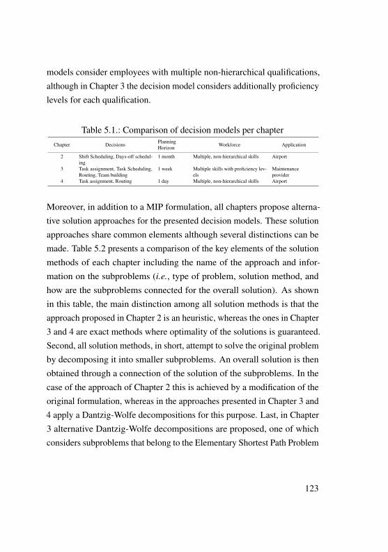
models consider employees with multiple non-hierarchical qualifications,although in Chapter 3 the decision model considers additionally proficiencylevels for each qualification.

Table 5.1.: Comparison of decision models per chapterChapter Decisions Planning Workforce ApplicationHorizon

2 Shift Scheduling, Days-off schedul-ing

1 month Multiple, non-hierarchical skills Airport

3 Task assignment, Task Scheduling,Routing, Team building

1 week Multiple skills with proficiency lev-els

Maintenanceprovider

4 Task assignment, Routing 1 day Multiple, non-hierarchical skills Airport

Moreover, in addition to a MIP formulation, all chapters propose alterna-tive solution approaches for the presented decision models. These solutionapproaches share common elements although several distinctions can bemade. Table 5.2 presents a comparison of the key elements of the solutionmethods of each chapter including the name of the approach and infor-mation on the subproblems (i.e., type of problem, solution method, andhow are the subproblems connected for the overall solution). As shownin this table, the main distinction among all solution methods is that theapproach proposed in Chapter 2 is an heuristic, whereas the ones in Chapter3 and 4 are exact methods where optimality of the solutions is guaranteed.Second, all solution methods, in short, attempt to solve the original problemby decomposing it into smaller subproblems. An overall solution is thenobtained through a connection of the solution of the subproblems. In thecase of the approach of Chapter 2 this is achieved by a modification of theoriginal formulation, whereas in the approaches presented in Chapter 3 and4 apply a Dantzig-Wolfe decompositions for this purpose. Last, in Chapter3 alternative Dantzig-Wolfe decompositions are proposed, one of whichconsiders subproblems that belong to the Elementary Shortest Path Problem

123

with Resource Constraints (ESPPRC) class. The approach presented inChapter 4, however, exploits certain characteristics of the problem at handto formulate the subproblems as Shortest Path Problems with ResourceConstraints (SPPRC), which require less computational effort for theirsolution.

Table 5.2.: Comparison of solution methods per chapterChapter Approach Subproblems

Type Solution Connection

2 Rolling PlanningHorizon heuristic

Reduced version of originalproblem

MIP solver Modified tour building con-straints

3 Branch-and-price 1) Reduced version of origi-nal problem

1) MIP solver 1) Master problem solvedwith Column Generation

2) Elementary Shortest Pathwith Resource Constaints(ESPPRC)

2) Labeling algorithm 2) Master problem solvedwith Column Generation

4 Branch-and-price Shortest Path with ResourceConstraints (SPPRC)

Labeling algorithm Master problem solved withColumn Generation

5.2. Further research directionsNotwithstanding that the presented scheduling problems correspond todifferent stages of the workforce scheduling process, future research can beoriented towards their integration into a single decision support system. Oneoption can be to integrate them in a hierarchical planning framework, wherethat problems are solved sequentially with information links to connectthem. Likewise, another integration option can be to incorporate severaldecisions of different problems into the formulation of a single decisionmodel.

As all presented decision models are workforce related, further researchcan be oriented to common directions such as incorporating employeespreferences, fairness, workload balance, meal-break placements, etc. Onthe other hand, all models from this thesis assume information is determin-

124

istic and known in advance. Hence, robust optimization approaches needto be developed in order to accommodate for the stochastic effects of theinformation.

In relation to the solution approaches proposed in this thesis, future re-search is required for an improvement in their performance. In the caseof Chapter 2, alternative solution approaches (e.g., tabu search, simulatedannealing, etc.) can be developed for solving the subproblems of the rollinghorizon-based heuristic. For Chapter 3 and 4, alternative ideas from exist-ing solution approaches for similar routing problems can be implemented.Such ideas include, for example, the implementation acceleration and stabi-lization strategies in the column generation phase of the algorithms, or theimplementation of ng-paths (Baldacci et al., 2011), bi-directional labeling(Liberatore et al., 2010) or hybrid methods (Gendreau et al., 2016) for thesolution of the subproblems.

Since scheduling problems can be found in more areas of application thanthose mentioned in this thesis, further research involves transferring theproposed solution approaches to scheduling problems in other applications(e.g., job-shop scheduling, production scheduling with sequence-dependentsetup times, etc.).

125

Bibliography

Airport Research Center (2009). Study on the Impact of Directive 96/67/ECon Ground Handling Services 1996-2007. Aachen.

Akjiratikarl, C., P. Yenradee, and P. R. Drake (2007). Pso-based algorithmfor home care worker scheduling in the uk. Computers & IndustrialEngineering 53(4), 559–583.

Alfares, H. K. (2004). Survey, Categorization, and Comparison of RecentTour Scheduling Literature. Annals of Operations Research 127(1-4),145–175.

Baker, K. (1977). An experimental study of the effectiveness of rollingschedules in production planning. Decision Sciences 8(1), 19–27.

Baker, K. and D. Peterson (1979). An analytic framework for evaluatingrolling schedules. Management Science 25(4), 341–351.

Baldacci, R., A. Mingozzi, and R. Roberti (2011). New route relaxationand pricing strategies for the vehicle routing problem. Operations re-search 59(5), 1269–1283.

Bard, J. F. and H. W. Purnomo (2005). Hospital-wide reactive scheduling ofnurses with preference considerations. IIE Transactions 37(7), 589–608.

XVII

Barnhart, C., E. L. Johnson, G. L. Nemhauser, M. W. Savelsbergh, and P. H.Vance (1998). Branch-and-price: Column generation for solving hugeinteger programs. Operations research 46(3), 316–329.

Barrera, D., N. Velasco, and C.-A. Amaya (2012). A network-basedapproach to the multi-activity combined timetabling and crew schedulingproblem: Workforce scheduling for public health policy implementation.Computers & Industrial Engineering 63(4), 802–812.

Bartholdi, J. J. I. (1981). A guaranteed-accuracy round-off algorithm forcyclic scheduling and set covering. Operations Research 29(3), 501–510.

Bertels, S. and T. Fahle (2006). A hybrid setup for a hybrid scenario:combining heuristics for the home health care problem. Computers &Operations Research 33(10), 2866–2890.

Blakeley, F., B. Arguello, B. Cao, W. Hall, and J. Knolmajer (2003). Opti-mizing Periodic Maintenance Operations for Schindler Elevator Corpo-ration. Interfaces 33(1), 67–79.

Bode, C. and S. Irnich (2014a). The shortest-path problem with resourceconstraints with (k,2)-loop elimination and its application to the ca-pacitated arc-routing problem. European Journal of Operational Re-search 238(2), 415–426.

Bode, C. and S. Irnich (2014b). The shortest-path problem with resourceconstraints with -loop elimination and its application to the capacitatedarc-routing problem. European Journal of Operational Research 238(2),415–426.

Bostel, N., P. Dejax, P. Guez, and F. Tricoire (2008). Multiperiod Planningand Routing on a Rolling Horizon for Field Force Optimization Logistics.

XVIII

In B. Golden, S. Raghavan, and E. Wasil (Eds.), The Vehicle RoutingProblem: Latest Advances and New Challenges, Volume 43 of Opera-tions Research/Computer Science Interfaces, Chapter 3, pp. 503–525.Boston, MA: Springer US.

Boussier, S., D. Feillet, and M. Gendreau (2006). An exact algorithm forteam orienteering problems. 4OR 5(3), 211–230.

Campbell, G. M. (1999). Cross-utilization of workers whose capabilitiesdiffer. Management Science 45(5), 722–732.

Campbell, G. M. and M. Diaby (2002). Development and evaluation ofan assignment heuristic for allocating cross-trained workers. EuropeanJournal of Operational Research 138(1), 9–20.

Caseau, Y. and P. Koppstein (1992). A cooperative-architecture expertsystem for solving large time/travel assignment problems. In Databaseand Expert Systems Applications, pp. 197–202. Springer.

Castillo-Salazar, J. A., D. Landa-Silva, and R. Qu (2014). Workforcescheduling and routing problems: literature survey and computationalstudy. Annals of Operations Research, 1–29.

Cheng, E. and J. L. Rich (1998, 04). A home health care routing andscheduling problem. Technical report, Rice University.

Choi, E. and D.-W. Tcha (2007). A column generation approach to theheterogeneous fleet vehicle routing problem. Computers & OperationsResearch 34(7), 2080–2095.

Cordeau, J.-F., G. Desaulniers, J. Desrosiers, M. M. Solomon, andF. Soumis (2001). The VRP with time windows. In P. Toth and D. Vigo

XIX

(Eds.), The vehicle routing problem, pp. 157–193. Society for Industrialand Applied Mathematics.

Cordeau, J.-F., G. Laporte, F. Pasin, and S. Ropke (2010a). Schedulingtechnicians and tasks in a telecommunications company. Journal ofScheduling 13(4), 393–409.

Cordeau, J.-F., G. Laporte, F. Pasin, and S. Ropke (2010b). Schedulingtechnicians and tasks in a telecommunications company. Journal ofScheduling 13(4), 393–409.

Corominas, A., J. Olivella, and R. Pastor (2010). A model for the as-signment of a set of tasks when work performance depends on expe-rience of all tasks involved. International Journal of Production Eco-nomics 126(2), 335–340.

Corominas, A., R. Pastor, and E. Rodrıguez (2006). Rotational allocationof tasks to multifunctional workers in a service industry. InternationalJournal of Production Economics 103(1), 3–9.

Dantzig, G. (1954). A Comment on Edie’s “Traffic Delays at Toll Booths”.Journal of the Operations Research Society of America 2(3), 339–341.

Day, P. R. and D. M. Ryan (1997). Flight attendant rostering for short-haulairline operations. Operations Research 45(5), 649–661.

Desrochers, M., J. Desrosiers, and M. M. Solomon (1992). A new opti-mization algorithm for the vehicle routing problem with time windows.Operations Research 40(2), 342–354.

Dohn, A., E. Kolind, and J. Clausen (2009a). The manpower allocationproblem with time windows and job-teaming constraints: A branch-and-price approach. Computers & Operations Research 36(4), 1145–1157.

XX

Dohn, A., E. Kolind, and J. Clausen (2009b). The manpower allocationproblem with time windows and job-teaming constraints: A branch-and-price approach. Computers & Operations Research 36(4), 1145–1157.

Dror, M. (1994). Note on the complexity of the shortest path models forcolumn generation in VRPTW. Operations Research 42(5), 977–978.

Edison, E. and T. Shima (2011). Integrated task assignment and pathoptimization for cooperating uninhabited aerial vehicles using geneticalgorithms. Computers & Operations Research 38(1), 340–356.

Eitzen, G., D. Panton, and G. Mills (2004). Multi-Skilled WorkforceOptimisation. Annals of Operations Research 127(1-4), 359–372.

Ernst, A., H. Jiang, and M. Krishnamoorthy (2004a). An annotated bibli-ography of personnel scheduling and rostering. Annals of OperationsResearch 127(1-4), 21–144.

Ernst, A., H. Jiang, and M. Krishnamoorthy (2004b). Staff scheduling androstering: A review of applications, methods and models. EuropeanJournal of Operational Research 153(1), 3–27.

Eveborn, P., P. Flisberg, and M. Ronnqvist (2006a). LAPS CARE - Anoperational system for staff planning of home care. European Journal ofOperational Research 171(3), 962–976.

Eveborn, P., P. Flisberg, and M. Ronnqvist (2006b). Laps care- an oper-ational system for staff planning of home care. European Journal ofOperational Research 171(3), 962–976.

Feillet, D. (2010). A tutorial on column generation and branch-and-pricefor vehicle routing problems. 4OR 8, 407–424.

XXI

Feillet, D., P. Dejax, M. Gendreau, and C. Gueguen (2004). An exactalgorithm for the elementary shortest path problem with resource con-straints: Application to some vehicle routing problems. Networks 44(3),216–229.

Ferland, J. A. and P. Michelon (1988). The vehicle scheduling problemwith multiple vehicle types. Journal of the Operational Research Soci-ety 39(6), 577–583.

Francis, P., K. Smilowitz, and M. Tzur (2006). The period vehicle routingproblem with service choice. Transportation Science 40(4), 439–454.

Francis, P. M., K. R. Smilowitz, and M. Tzur (2008). The Period VehicleRouting Problem and its Extensions. In B. Golden, S. Raghavan, andE. Wasil (Eds.), The Vehicle Routing Problem: Latest Advances andNew Challenges, Volume 43 of Operations Research/Computer ScienceInterfaces, Chapter 1, pp. 73–102. Boston, MA: Springer US.

Gendreau, M., D. Manerba, and R. Mansini (2016). The multi-vehicletraveling purchaser problem with pairwise incompatibility constraintsand unitary demands: A branch-and-price approach. European Journalof Operational Research 248(1), 59–71.

Google (2016). The Google Maps Distance Matrix API. https:

//developers.google.com/maps/documentation/

distance-matrix/intro.

Goossens, D., S. Polyakovskiy, F. C. R. Spieksma, and G. J. Woeginger(2012). Between a rock and a hard place: the two-to-one assignmentproblem. Mathematical Methods of Operations Research 76(2), 223–237.

XXII

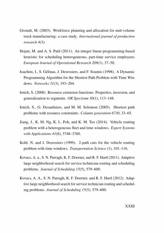
Gronalt, M. (2003). Workforce planning and allocation for mid-volumetruck manufacturing: a case study. International journal of productionresearch 4(3).

Hojati, M. and A. S. Patil (2011). An integer linear programming-basedheuristic for scheduling heterogeneous, part-time service employees.European Journal of Operational Research 209(1), 37–50.

Ioachim, I., S. Gelinas, J. Desrosiers, and F. Soumis (1998). A DynamicProgramming Algorithm for the Shortest Path Problem with Time Win-dows. Networks 31(3), 193–204.

Irnich, S. (2008). Resource extension functions: Properties, inversion, andgeneralization to segments. OR Spectrum 30(1), 113–148.

Irnich, S., G. Desaulniers, and M. M. Solomon (2005). Shortest pathproblems with resource constraints. Column generation 6730, 33–65.

Jiang, J., K. M. Ng, K. L. Poh, and K. M. Teo (2014). Vehicle routingproblem with a heterogeneous fleet and time windows. Expert Systemswith Applications 41(8), 3748–3760.

Kohl, N. and J. Desrosiers (1999). 2-path cuts for the vehicle routingproblem with time windows. Transportation Science (1), 101–116.

Kovacs, A. a., S. N. Parragh, K. F. Doerner, and R. F. Hartl (2011). Adaptivelarge neighborhood search for service technician routing and schedulingproblems. Journal of Scheduling 15(5), 579–600.

Kovacs, A. A., S. N. Parragh, K. F. Doerner, and R. F. Hartl (2012). Adap-tive large neighborhood search for service technician routing and schedul-ing problems. Journal of Scheduling 15(5), 579–600.

XXIII

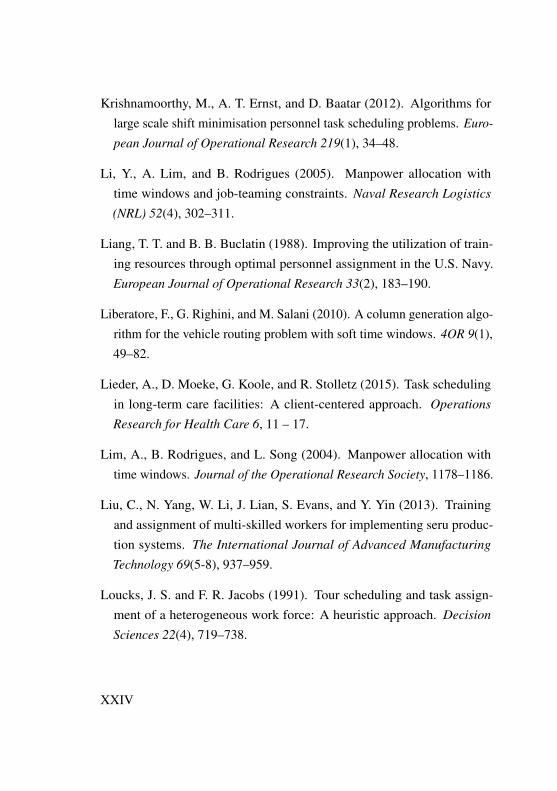
Krishnamoorthy, M., A. T. Ernst, and D. Baatar (2012). Algorithms forlarge scale shift minimisation personnel task scheduling problems. Euro-pean Journal of Operational Research 219(1), 34–48.

Li, Y., A. Lim, and B. Rodrigues (2005). Manpower allocation withtime windows and job-teaming constraints. Naval Research Logistics(NRL) 52(4), 302–311.

Liang, T. T. and B. B. Buclatin (1988). Improving the utilization of train-ing resources through optimal personnel assignment in the U.S. Navy.European Journal of Operational Research 33(2), 183–190.

Liberatore, F., G. Righini, and M. Salani (2010). A column generation algo-rithm for the vehicle routing problem with soft time windows. 4OR 9(1),49–82.

Lieder, A., D. Moeke, G. Koole, and R. Stolletz (2015). Task schedulingin long-term care facilities: A client-centered approach. OperationsResearch for Health Care 6, 11 – 17.

Lim, A., B. Rodrigues, and L. Song (2004). Manpower allocation withtime windows. Journal of the Operational Research Society, 1178–1186.

Liu, C., N. Yang, W. Li, J. Lian, S. Evans, and Y. Yin (2013). Trainingand assignment of multi-skilled workers for implementing seru produc-tion systems. The International Journal of Advanced ManufacturingTechnology 69(5-8), 937–959.

Loucks, J. S. and F. R. Jacobs (1991). Tour scheduling and task assign-ment of a heterogeneous work force: A heuristic approach. DecisionSciences 22(4), 719–738.

XXIV

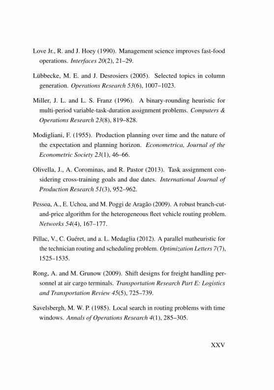
Love Jr., R. and J. Hoey (1990). Management science improves fast-foodoperations. Interfaces 20(2), 21–29.

Lubbecke, M. E. and J. Desrosiers (2005). Selected topics in columngeneration. Operations Research 53(6), 1007–1023.

Miller, J. L. and L. S. Franz (1996). A binary-rounding heuristic formulti-period variable-task-duration assignment problems. Computers &Operations Research 23(8), 819–828.

Modigliani, F. (1955). Production planning over time and the nature ofthe expectation and planning horizon. Econometrica, Journal of theEconometric Society 23(1), 46–66.

Olivella, J., A. Corominas, and R. Pastor (2013). Task assignment con-sidering cross-training goals and due dates. International Journal ofProduction Research 51(3), 952–962.

Pessoa, A., E. Uchoa, and M. Poggi de Aragao (2009). A robust branch-cut-and-price algorithm for the heterogeneous fleet vehicle routing problem.Networks 54(4), 167–177.

Pillac, V., C. Gueret, and a. L. Medaglia (2012). A parallel matheuristic forthe technician routing and scheduling problem. Optimization Letters 7(7),1525–1535.

Rong, A. and M. Grunow (2009). Shift designs for freight handling per-sonnel at air cargo terminals. Transportation Research Part E: Logisticsand Transportation Review 45(5), 725–739.

Savelsbergh, M. W. P. (1985). Local search in routing problems with timewindows. Annals of Operations Research 4(1), 285–305.

XXV

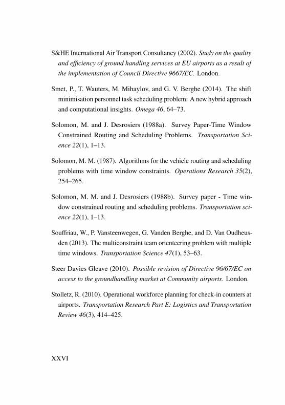
S&HE International Air Transport Consultancy (2002). Study on the qualityand efficiency of ground handling services at EU airports as a result ofthe implementation of Council Directive 9667/EC. London.

Smet, P., T. Wauters, M. Mihaylov, and G. V. Berghe (2014). The shiftminimisation personnel task scheduling problem: A new hybrid approachand computational insights. Omega 46, 64–73.

Solomon, M. and J. Desrosiers (1988a). Survey Paper-Time WindowConstrained Routing and Scheduling Problems. Transportation Sci-ence 22(1), 1–13.

Solomon, M. M. (1987). Algorithms for the vehicle routing and schedulingproblems with time window constraints. Operations Research 35(2),254–265.

Solomon, M. M. and J. Desrosiers (1988b). Survey paper - Time win-dow constrained routing and scheduling problems. Transportation sci-ence 22(1), 1–13.

Souffriau, W., P. Vansteenwegen, G. Vanden Berghe, and D. Van Oudheus-den (2013). The multiconstraint team orienteering problem with multipletime windows. Transportation Science 47(1), 53–63.

Steer Davies Gleave (2010). Possible revision of Directive 96/67/EC onaccess to the groundhandling market at Community airports. London.

Stolletz, R. (2010). Operational workforce planning for check-in counters atairports. Transportation Research Part E: Logistics and TransportationReview 46(3), 414–425.

XXVI

Stolletz, R. and E. Zamorano (2014). A rolling planning horizon heuris-tic for scheduling agents with different qualifications. TransportationResearch Part E: Logistics and Transportation Review 68, 39 – 52.

Tang, H., E. Millerhooks, and R. Tomastik (2007). Scheduling techniciansfor planned maintenance of geographically distributed equipment. Trans-portation Research Part E: Logistics and Transportation Review 43(5),591–609.

The World Bank (2016). Compensation of employees (% of expense).World Data Bank: http://databank.worldbank.org/.

Tsang, E. and C. Voudouris (1997). Fast local search and guided localsearch and their application to British Telecom’s workforce schedulingproblem. Operations Research Letters 20(3), 119–127.

Van den Bergh, J., J. Belien, P. De Bruecker, E. Demeulemeester, and L. DeBoeck (2013). Personnel scheduling: A literature review. EuropeanJournal of Operational Research 226(3), 367 – 385.

Xu, J. and S. Chiu (2001). Effective heuristic procedures for a field techni-cian scheduling problem. Journal of Heuristics 7(5), 495–509.

Yang, R. (1996). Solving a workforce management problem with constraintprogramming. In The 2nd International Conference on the PracticalApplication of Constraint Technology, pp. 373–387. The Practical Appli-cation Company Ltd.

XXVII

A. Realistic instances from Chapter 4

In the following section detailed informations on realistic instances A1-A4 is presented. Tables A.1 to A.4 show the task index, the counteropening time, the occupation time (in minutes), the agent requirements,and the skills required. Tables A.5 to A.8 present information regardingthe workforce, including: agent index, qualifications, shift start time, andshift end time. Last, tables A.9 to A.12 display the travel time (in minutes)from and to each task (including depot). This information is available athttp://stolletz.bwl.uni-mannheim.de/en/library.

We also use the following values for the remaining parameters:

• w

max

ik

= 0.5 · (bi

� a

i

) 8i 2 I , 8k 2 K

• out

max

i

= v

i

� 1 8i 2 I

• The maximum overtime per agent is set such that the shift lengthplus overtime cannot exceed 10 hours.

• [↵1,↵2,↵3,↵4] = [0.1, 0.2, 0.3, 0.4]

• 1 hour computation time limit

XXIX

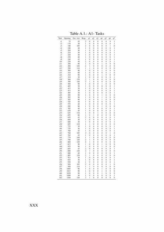
Table A.1.: A1- TasksTask Opening Occ. (m) Reqs. q1 q2 q3 q4 q5 q6 q7

i1 75 45 2 0 0 0 0 0 0 1i2 170 30 1 0 0 0 0 0 0 1i3 180 105 2 0 0 0 0 0 1 0i4 180 40 1 0 0 0 0 0 0 1i5 200 30 1 0 0 0 0 0 0 1i6 210 30 1 0 0 0 0 0 0 1i7 220 30 1 0 0 0 0 0 0 1i8 230 40 1 0 0 0 0 0 0 1i9 240 45 1 0 0 0 0 0 0 1

i10 250 40 2 0 0 0 0 0 0 1i11 290 90 1 0 0 0 1 0 0 0i12 290 120 2 1 0 0 0 0 0 0i13 290 110 1 1 0 0 0 0 0 0i14 300 90 1 0 0 0 1 0 0 0i15 310 80 1 0 0 0 0 0 1 0i16 310 90 1 0 0 0 1 0 0 0i17 310 30 1 0 0 0 0 0 0 1i18 360 120 2 1 0 0 0 0 0 0i19 390 140 2 1 0 0 0 0 0 0i20 400 90 1 0 0 0 1 0 0 0i21 405 30 1 0 0 0 0 0 0 1i22 415 30 1 0 0 0 0 0 0 1i23 415 30 1 0 0 0 0 0 0 1i24 495 30 1 0 0 0 0 0 0 1i25 495 90 1 0 0 0 1 0 0 0i26 505 90 1 0 0 0 1 0 0 0i27 505 90 1 0 0 0 1 0 0 0i28 525 40 1 0 0 0 0 0 0 1i29 575 40 1 0 0 0 0 0 0 1i30 585 90 1 0 0 0 1 0 0 0i31 585 40 1 0 0 0 0 0 0 1i32 630 40 1 0 0 0 0 0 0 1i33 635 110 1 0 0 1 0 0 0 0i34 655 80 1 0 1 0 0 0 0 0i35 655 45 2 0 0 0 0 0 0 1i36 660 30 1 0 0 0 0 0 0 1i37 680 30 1 0 0 0 0 0 0 1i38 695 110 1 1 0 0 0 0 0 0i39 725 30 1 0 0 0 0 0 0 1i40 735 30 1 0 0 0 0 0 0 1i41 760 45 1 0 0 0 0 0 0 1i42 760 105 2 0 0 0 0 0 1 0i43 765 45 1 0 0 0 0 0 0 1i44 770 140 1 1 0 0 0 0 0 0i45 780 120 2 1 0 0 0 0 0 0i46 800 120 2 1 0 0 0 0 0 0i47 815 90 1 0 0 0 1 0 0 0i48 825 90 1 0 0 0 1 0 0 0i49 845 45 2 0 0 0 0 0 0 1i50 880 120 2 1 0 0 0 0 0 0i51 880 40 1 0 0 0 0 0 0 1i52 885 120 2 1 0 0 0 0 0 0i53 915 30 1 0 0 0 0 0 0 1i54 925 30 1 0 0 0 0 0 0 1i55 930 30 1 0 0 0 0 0 0 1i56 950 105 2 0 0 0 0 0 1 0i57 990 110 1 1 0 0 0 0 0 0i58 1005 90 1 0 0 0 1 0 0 0i59 1015 90 1 0 0 0 1 0 0 0i60 1020 90 1 0 0 0 1 0 0 0i61 1080 30 1 0 0 0 0 0 0 1i62 1200 120 2 1 0 0 0 0 0 0

XXX

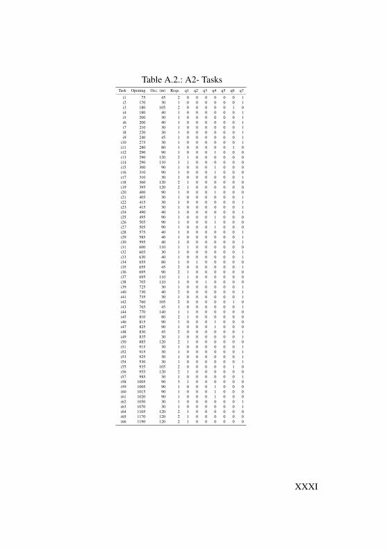
Table A.2.: A2- TasksTask Opening Occ. (m) Reqs. q1 q2 q3 q4 q5 q6 q7

i1 75 45 2 0 0 0 0 0 0 1i2 170 30 1 0 0 0 0 0 0 1i3 180 105 2 0 0 0 0 0 1 0i4 180 40 1 0 0 0 0 0 0 1i5 200 30 1 0 0 0 0 0 0 1i6 200 40 1 0 0 0 0 0 0 1i7 210 30 1 0 0 0 0 0 0 1i8 220 30 1 0 0 0 0 0 0 1i9 240 45 1 0 0 0 0 0 0 1

i10 275 30 1 0 0 0 0 0 0 1i11 280 80 1 0 0 0 0 0 1 0i12 290 90 1 0 0 0 1 0 0 0i13 290 120 2 1 0 0 0 0 0 0i14 290 110 1 1 0 0 0 0 0 0i15 300 90 1 0 0 0 1 0 0 0i16 310 90 1 0 0 0 1 0 0 0i17 310 30 1 0 0 0 0 0 0 1i18 360 120 2 1 0 0 0 0 0 0i19 395 120 2 1 0 0 0 0 0 0i20 400 90 1 0 0 0 1 0 0 0i21 405 30 1 0 0 0 0 0 0 1i22 415 30 1 0 0 0 0 0 0 1i23 415 30 1 0 0 0 0 0 0 1i24 490 40 1 0 0 0 0 0 0 1i25 495 90 1 0 0 0 1 0 0 0i26 505 90 1 0 0 0 1 0 0 0i27 505 90 1 0 0 0 1 0 0 0i28 575 40 1 0 0 0 0 0 0 1i29 585 40 1 0 0 0 0 0 0 1i30 595 40 1 0 0 0 0 0 0 1i31 600 110 1 1 0 0 0 0 0 0i32 605 30 1 0 0 0 0 0 0 1i33 630 40 1 0 0 0 0 0 0 1i34 655 80 1 0 1 0 0 0 0 0i35 655 45 2 0 0 0 0 0 0 1i36 695 90 2 1 0 0 0 0 0 0i37 695 110 1 1 0 0 0 0 0 0i38 705 110 1 0 0 1 0 0 0 0i39 725 30 1 0 0 0 0 0 0 1i40 730 40 2 0 0 0 0 0 0 1i41 735 30 1 0 0 0 0 0 0 1i42 760 105 2 0 0 0 0 0 1 0i43 765 45 1 0 0 0 0 0 0 1i44 770 140 1 1 0 0 0 0 0 0i45 810 80 2 1 0 0 0 0 0 0i46 815 90 1 0 0 0 1 0 0 0i47 825 90 1 0 0 0 1 0 0 0i48 830 45 2 0 0 0 0 0 0 1i49 835 30 1 0 0 0 0 0 0 1i50 885 120 2 1 0 0 0 0 0 0i51 915 30 1 0 0 0 0 0 0 1i52 915 30 1 0 0 0 0 0 0 1i53 925 30 1 0 0 0 0 0 0 1i54 930 30 1 0 0 0 0 0 0 1i55 935 105 2 0 0 0 0 0 1 0i56 955 120 2 1 0 0 0 0 0 0i57 985 30 1 0 0 0 0 0 0 1i58 1005 90 3 1 0 0 0 0 0 0i59 1005 90 1 0 0 0 1 0 0 0i60 1015 90 1 0 0 0 1 0 0 0i61 1020 90 1 0 0 0 1 0 0 0i62 1050 30 1 0 0 0 0 0 0 1i63 1070 30 1 0 0 0 0 0 0 1i64 1105 120 2 1 0 0 0 0 0 0i65 1170 120 2 1 0 0 0 0 0 0i66 1190 120 2 1 0 0 0 0 0 0

XXXI

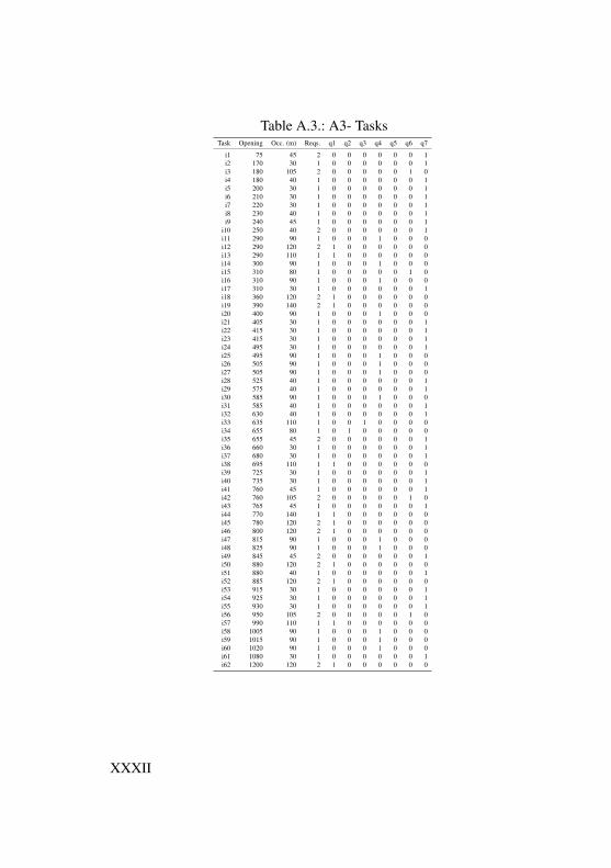
Table A.3.: A3- TasksTask Opening Occ. (m) Reqs. q1 q2 q3 q4 q5 q6 q7

i1 75 45 2 0 0 0 0 0 0 1i2 170 30 1 0 0 0 0 0 0 1i3 180 105 2 0 0 0 0 0 1 0i4 180 40 1 0 0 0 0 0 0 1i5 200 30 1 0 0 0 0 0 0 1i6 210 30 1 0 0 0 0 0 0 1i7 220 30 1 0 0 0 0 0 0 1i8 230 40 1 0 0 0 0 0 0 1i9 240 45 1 0 0 0 0 0 0 1

i10 250 40 2 0 0 0 0 0 0 1i11 290 90 1 0 0 0 1 0 0 0i12 290 120 2 1 0 0 0 0 0 0i13 290 110 1 1 0 0 0 0 0 0i14 300 90 1 0 0 0 1 0 0 0i15 310 80 1 0 0 0 0 0 1 0i16 310 90 1 0 0 0 1 0 0 0i17 310 30 1 0 0 0 0 0 0 1i18 360 120 2 1 0 0 0 0 0 0i19 390 140 2 1 0 0 0 0 0 0i20 400 90 1 0 0 0 1 0 0 0i21 405 30 1 0 0 0 0 0 0 1i22 415 30 1 0 0 0 0 0 0 1i23 415 30 1 0 0 0 0 0 0 1i24 495 30 1 0 0 0 0 0 0 1i25 495 90 1 0 0 0 1 0 0 0i26 505 90 1 0 0 0 1 0 0 0i27 505 90 1 0 0 0 1 0 0 0i28 525 40 1 0 0 0 0 0 0 1i29 575 40 1 0 0 0 0 0 0 1i30 585 90 1 0 0 0 1 0 0 0i31 585 40 1 0 0 0 0 0 0 1i32 630 40 1 0 0 0 0 0 0 1i33 635 110 1 0 0 1 0 0 0 0i34 655 80 1 0 1 0 0 0 0 0i35 655 45 2 0 0 0 0 0 0 1i36 660 30 1 0 0 0 0 0 0 1i37 680 30 1 0 0 0 0 0 0 1i38 695 110 1 1 0 0 0 0 0 0i39 725 30 1 0 0 0 0 0 0 1i40 735 30 1 0 0 0 0 0 0 1i41 760 45 1 0 0 0 0 0 0 1i42 760 105 2 0 0 0 0 0 1 0i43 765 45 1 0 0 0 0 0 0 1i44 770 140 1 1 0 0 0 0 0 0i45 780 120 2 1 0 0 0 0 0 0i46 800 120 2 1 0 0 0 0 0 0i47 815 90 1 0 0 0 1 0 0 0i48 825 90 1 0 0 0 1 0 0 0i49 845 45 2 0 0 0 0 0 0 1i50 880 120 2 1 0 0 0 0 0 0i51 880 40 1 0 0 0 0 0 0 1i52 885 120 2 1 0 0 0 0 0 0i53 915 30 1 0 0 0 0 0 0 1i54 925 30 1 0 0 0 0 0 0 1i55 930 30 1 0 0 0 0 0 0 1i56 950 105 2 0 0 0 0 0 1 0i57 990 110 1 1 0 0 0 0 0 0i58 1005 90 1 0 0 0 1 0 0 0i59 1015 90 1 0 0 0 1 0 0 0i60 1020 90 1 0 0 0 1 0 0 0i61 1080 30 1 0 0 0 0 0 0 1i62 1200 120 2 1 0 0 0 0 0 0

XXXII

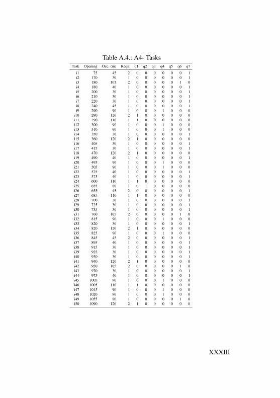
Table A.4.: A4- TasksTask Opening Occ. (m) Reqs. q1 q2 q3 q4 q5 q6 q7

i1 75 45 2 0 0 0 0 0 0 1i2 170 30 1 0 0 0 0 0 0 1i3 180 105 2 0 0 0 0 0 1 0i4 180 40 1 0 0 0 0 0 0 1i5 200 30 1 0 0 0 0 0 0 1i6 210 30 1 0 0 0 0 0 0 1i7 220 30 1 0 0 0 0 0 0 1i8 240 45 1 0 0 0 0 0 0 1i9 290 90 1 0 0 0 1 0 0 0

i10 290 120 2 1 0 0 0 0 0 0i11 290 110 1 1 0 0 0 0 0 0i12 300 90 1 0 0 0 1 0 0 0i13 310 90 1 0 0 0 1 0 0 0i14 350 30 1 0 0 0 0 0 0 1i15 360 120 2 1 0 0 0 0 0 0i16 405 30 1 0 0 0 0 0 0 1i17 415 30 1 0 0 0 0 0 0 1i18 470 120 2 1 0 0 0 0 0 0i19 490 40 1 0 0 0 0 0 0 1i20 495 90 1 0 0 0 1 0 0 0i21 505 90 1 0 0 0 1 0 0 0i22 575 40 1 0 0 0 0 0 0 1i23 575 40 1 0 0 0 0 0 0 1i24 600 110 1 1 0 0 0 0 0 0i25 655 80 1 0 1 0 0 0 0 0i26 655 45 2 0 0 0 0 0 0 1i27 685 110 1 1 0 0 0 0 0 0i28 700 30 1 0 0 0 0 0 0 1i29 725 30 1 0 0 0 0 0 0 1i30 735 30 1 0 0 0 0 0 0 1i31 760 105 2 0 0 0 0 0 1 0i32 815 90 1 0 0 0 1 0 0 0i33 820 30 1 0 0 0 0 0 0 1i34 820 120 2 1 0 0 0 0 0 0i35 825 90 1 0 0 0 1 0 0 0i36 845 45 2 0 0 0 0 0 0 1i37 895 40 1 0 0 0 0 0 0 1i38 915 30 1 0 0 0 0 0 0 1i39 925 30 1 0 0 0 0 0 0 1i40 930 30 1 0 0 0 0 0 0 1i41 940 120 2 1 0 0 0 0 0 0i42 950 105 2 0 0 0 0 0 1 0i43 970 30 1 0 0 0 0 0 0 1i44 975 40 1 0 0 0 0 0 0 1i45 1005 90 1 0 0 0 1 0 0 0i46 1005 110 1 1 0 0 0 0 0 0i47 1015 90 1 0 0 0 1 0 0 0i48 1020 90 1 0 0 0 1 0 0 0i49 1055 80 1 0 0 0 0 0 1 0i50 1090 120 2 1 0 0 0 0 0 0

XXXIII

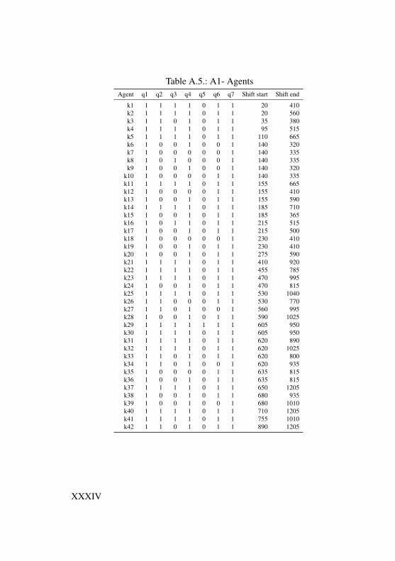
Table A.5.: A1- AgentsAgent q1 q2 q3 q4 q5 q6 q7 Shift start Shift end

k1 1 1 1 1 0 1 1 20 410k2 1 1 1 1 0 1 1 20 560k3 1 1 0 1 0 1 1 35 380k4 1 1 1 1 0 1 1 95 515k5 1 1 1 1 0 1 1 110 665k6 1 0 0 1 0 0 1 140 320k7 1 0 0 0 0 0 1 140 335k8 1 0 1 0 0 0 1 140 335k9 1 0 0 1 0 0 1 140 320

k10 1 0 0 0 0 1 1 140 335k11 1 1 1 1 0 1 1 155 665k12 1 0 0 0 0 1 1 155 410k13 1 0 0 1 0 1 1 155 590k14 1 1 1 1 0 1 1 185 710k15 1 0 0 1 0 1 1 185 365k16 1 0 1 1 0 1 1 215 515k17 1 0 0 1 0 1 1 215 500k18 1 0 0 0 0 0 1 230 410k19 1 0 0 1 0 1 1 230 410k20 1 0 0 1 0 1 1 275 590k21 1 1 1 1 0 1 1 410 920k22 1 1 1 1 0 1 1 455 785k23 1 1 1 1 0 1 1 470 995k24 1 0 0 1 0 1 1 470 815k25 1 1 1 1 0 1 1 530 1040k26 1 1 0 0 0 1 1 530 770k27 1 1 0 1 0 0 1 560 995k28 1 0 0 1 0 1 1 590 1025k29 1 1 1 1 1 1 1 605 950k30 1 1 1 1 0 1 1 605 950k31 1 1 1 1 0 1 1 620 890k32 1 1 1 1 0 1 1 620 1025k33 1 1 0 1 0 1 1 620 800k34 1 1 0 1 0 0 1 620 935k35 1 0 0 0 0 1 1 635 815k36 1 0 0 1 0 1 1 635 815k37 1 1 1 1 0 1 1 650 1205k38 1 0 0 1 0 1 1 680 935k39 1 0 0 1 0 0 1 680 1010k40 1 1 1 1 0 1 1 710 1205k41 1 1 1 1 0 1 1 755 1010k42 1 1 0 1 0 1 1 890 1205

XXXIV

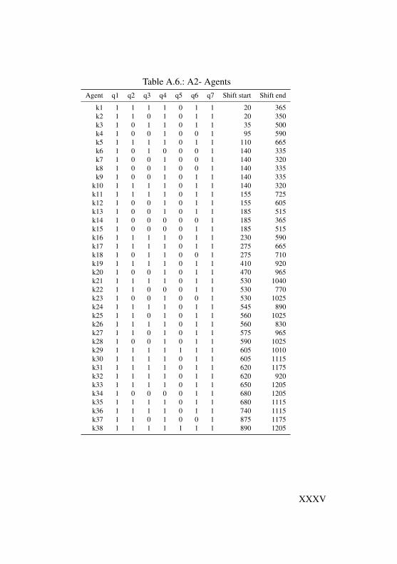
Table A.6.: A2- AgentsAgent q1 q2 q3 q4 q5 q6 q7 Shift start Shift end

k1 1 1 1 1 0 1 1 20 365k2 1 1 0 1 0 1 1 20 350k3 1 0 1 1 0 1 1 35 500k4 1 0 0 1 0 0 1 95 590k5 1 1 1 1 0 1 1 110 665k6 1 0 1 0 0 0 1 140 335k7 1 0 0 1 0 0 1 140 320k8 1 0 0 1 0 0 1 140 335k9 1 0 0 1 0 1 1 140 335

k10 1 1 1 1 0 1 1 140 320k11 1 1 1 1 0 1 1 155 725k12 1 0 0 1 0 1 1 155 605k13 1 0 0 1 0 1 1 185 515k14 1 0 0 0 0 0 1 185 365k15 1 0 0 0 0 1 1 185 515k16 1 1 1 1 0 1 1 230 590k17 1 1 1 1 0 1 1 275 665k18 1 0 1 1 0 0 1 275 710k19 1 1 1 1 0 1 1 410 920k20 1 0 0 1 0 1 1 470 965k21 1 1 1 1 0 1 1 530 1040k22 1 1 0 0 0 1 1 530 770k23 1 0 0 1 0 0 1 530 1025k24 1 1 1 1 0 1 1 545 890k25 1 1 0 1 0 1 1 560 1025k26 1 1 1 1 0 1 1 560 830k27 1 1 0 1 0 1 1 575 965k28 1 0 0 1 0 1 1 590 1025k29 1 1 1 1 1 1 1 605 1010k30 1 1 1 1 0 1 1 605 1115k31 1 1 1 1 0 1 1 620 1175k32 1 1 1 1 0 1 1 620 920k33 1 1 1 1 0 1 1 650 1205k34 1 0 0 0 0 1 1 680 1205k35 1 1 1 1 0 1 1 680 1115k36 1 1 1 1 0 1 1 740 1115k37 1 1 0 1 0 0 1 875 1175k38 1 1 1 1 1 1 1 890 1205

XXXV

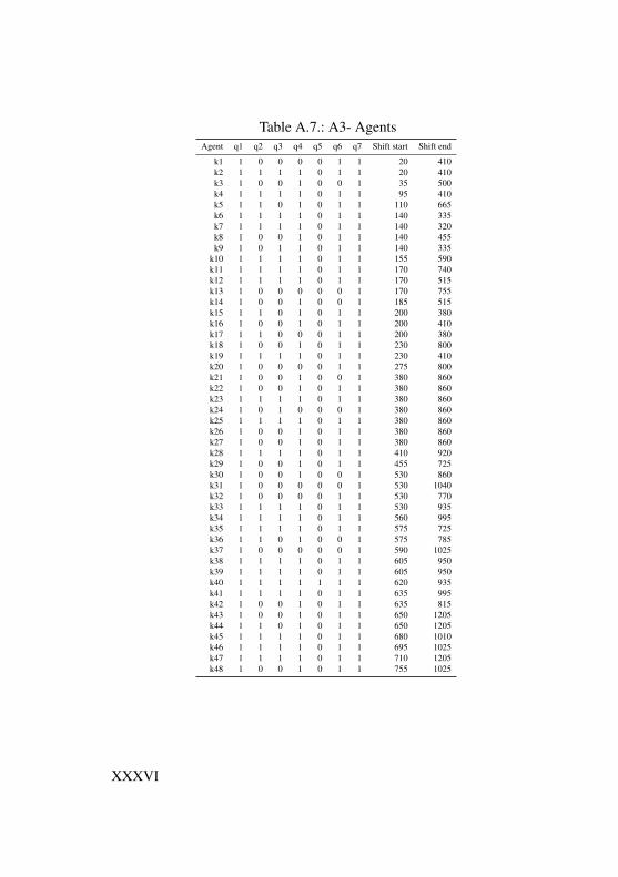
Table A.7.: A3- AgentsAgent q1 q2 q3 q4 q5 q6 q7 Shift start Shift end

k1 1 0 0 0 0 1 1 20 410k2 1 1 1 1 0 1 1 20 410k3 1 0 0 1 0 0 1 35 500k4 1 1 1 1 0 1 1 95 410k5 1 1 0 1 0 1 1 110 665k6 1 1 1 1 0 1 1 140 335k7 1 1 1 1 0 1 1 140 320k8 1 0 0 1 0 1 1 140 455k9 1 0 1 1 0 1 1 140 335

k10 1 1 1 1 0 1 1 155 590k11 1 1 1 1 0 1 1 170 740k12 1 1 1 1 0 1 1 170 515k13 1 0 0 0 0 0 1 170 755k14 1 0 0 1 0 0 1 185 515k15 1 1 0 1 0 1 1 200 380k16 1 0 0 1 0 1 1 200 410k17 1 1 0 0 0 1 1 200 380k18 1 0 0 1 0 1 1 230 800k19 1 1 1 1 0 1 1 230 410k20 1 0 0 0 0 1 1 275 800k21 1 0 0 1 0 0 1 380 860k22 1 0 0 1 0 1 1 380 860k23 1 1 1 1 0 1 1 380 860k24 1 0 1 0 0 0 1 380 860k25 1 1 1 1 0 1 1 380 860k26 1 0 0 1 0 1 1 380 860k27 1 0 0 1 0 1 1 380 860k28 1 1 1 1 0 1 1 410 920k29 1 0 0 1 0 1 1 455 725k30 1 0 0 1 0 0 1 530 860k31 1 0 0 0 0 0 1 530 1040k32 1 0 0 0 0 1 1 530 770k33 1 1 1 1 0 1 1 530 935k34 1 1 1 1 0 1 1 560 995k35 1 1 1 1 0 1 1 575 725k36 1 1 0 1 0 0 1 575 785k37 1 0 0 0 0 0 1 590 1025k38 1 1 1 1 0 1 1 605 950k39 1 1 1 1 0 1 1 605 950k40 1 1 1 1 1 1 1 620 935k41 1 1 1 1 0 1 1 635 995k42 1 0 0 1 0 1 1 635 815k43 1 0 0 1 0 1 1 650 1205k44 1 1 0 1 0 1 1 650 1205k45 1 1 1 1 0 1 1 680 1010k46 1 1 1 1 0 1 1 695 1025k47 1 1 1 1 0 1 1 710 1205k48 1 0 0 1 0 1 1 755 1025

XXXVI

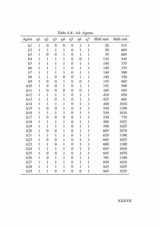
Table A.8.: A4- Agents

Agent q1 q2 q3 q4 q5 q6 q7 Shift start Shift end

k1 1 0 0 0 0 1 1 20 515k2 1 1 1 1 0 1 1 20 605k3 1 0 0 1 0 1 1 35 605k4 1 1 1 1 0 0 1 110 545k5 1 1 1 1 0 1 1 140 335k6 1 1 1 1 0 1 1 140 335k7 1 1 1 1 0 1 1 140 500k8 1 1 0 0 0 1 1 140 320k9 1 0 0 1 0 0 1 155 665

k10 1 0 0 1 0 1 1 155 590k11 1 0 0 0 0 0 1 185 695k12 1 1 1 1 0 1 1 410 920k13 1 1 0 1 0 1 1 425 605k14 1 1 1 1 0 1 1 440 1010k15 1 0 0 1 0 1 1 530 1100k16 1 1 1 1 0 1 1 530 1010k17 1 0 0 0 0 1 1 530 770k18 1 1 1 1 0 1 1 560 1025k19 1 1 1 1 0 1 1 590 1025k20 1 0 0 1 0 1 1 605 1070k21 1 1 1 1 0 1 1 620 1100k22 1 0 0 1 0 1 1 665 1025k23 1 1 0 1 0 1 1 680 1100k24 1 1 1 1 0 1 1 695 1010k25 1 0 0 1 0 1 1 695 1070k26 1 0 1 1 0 1 1 785 1100k27 1 1 1 1 0 1 1 830 1010k28 1 1 1 1 0 1 1 845 1025k29 1 1 0 1 0 0 1 845 1025

XXXVII

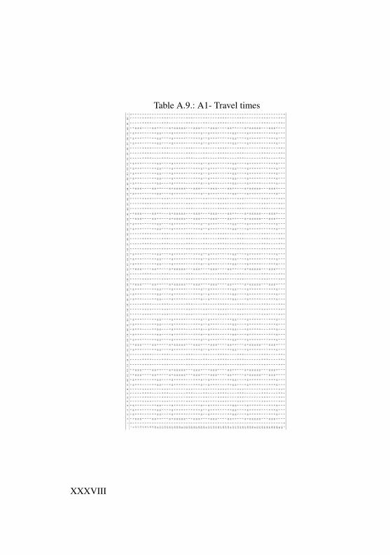
Table A.9.: A1- Travel times

oi1

i2i3

i4i5

i6i7

i8i9

i10

i11

i12

i13

i14

i15

i16

i17

i18

i19

i20

i21

i22

i23

i24

i25

i26

i27

i28

i29

i30

i31

i32

i33

i34

i35

i36

i37

i38

i39

i40

i41

i42

i43

i44

i45

i46

i47

i48

i49

i50

i51

i52

i53

i54

i55

i56

i57

i58

i59

i60

i61

i62

o

o0

55

55

55

55

55

55

55

55

55

55

55

55

55

55

55

55

55

55

55

55

55

55

55

55

55

55

55

55

55

55

55

0i1

50

1010

105

55

510

100

05

55

100

1010

1010

105

55

1010

100

55

010

1010

55

55

1010

00

55

510

010

1010

1010

55

510

1010

05

55

i25

100

00

55

55

00

1010

55

50

100

00

00

55

50

00

105

510

00

05

55

50

010

105

55

010

00

00

05

55

00

010

55

5i3

510

00

05

55

50

010

105

55

010

00

00

05

55

00

010

55

100

00

55

55

00

1010

55

50

100

00

00

55

50

00

105

55

i45

100

00

55

55

00

1010

55

50

100

00

00

55

50

00

105

510

00

05

55

50

010

105

55

010

00

00

05

55

00

010

55

5i5

55

55

50

00

05

55

50

00

55

55

55

50

00

55

55

00

55

55

00

00

55

55

00

05

55

55

55

00

05

55

50

05

i65

55

55

00

00

55

55

00

05

55

55

55

00

05

55

50

05

55

50

00

05

55

50

00

55

55

55

50

00

55

55

00

5i7

55

55

50

00

05

55

50

00

55

55

55

50

00

55

55

00

55

55

00

00

55

55

00

05

55

55

55

00

05

55

50

05

i85

55

55

00

00

55

55

00

05

55

55

55

00

05

55

50

05

55

50

00

05

55

50

00

55

55

55

50

00

55

55

00

5i9

510

00

05

55

50

010

105

55

010

00

00

05

55

00

010

55

100

00

55

55

00

1010

55

50

100

00

00

55

50

00

105

55

i10

510

00

05

55

50

010

105

55

010

00

00

05

55

00

010

55

100

00

55

55

00

1010

55

50

100

00

00

55

50

00

105

55

i11

50

1010

105

55

510

100

05

55

100

1010

1010

105

55

1010

100

55

010

1010

55

55

1010

00

55

510

010

1010

1010

55

510

1010

05

55

i12

50

1010

105

55

510

100

05

55

100

1010

1010

105

55

1010

100

55

010

1010

55

55

1010

00

55

510

010

1010

1010

55

510

1010

05

55

i13

55

55

50

00

05

55

50

00

55

55

55

50

00

55

55

00

55

55

00

00

55

55

00

05

55

55

55

00

05

55

50

05

i14

55

55

50

00

05

55

50

00

55

55

55

50

00

55

55

00

55

55

00

00

55

55

00

05

55

55

55

00

05

55

50

05

i15

55

55

50

00

05

55

50

00

55

55

55

50

00

55

55

00

55

55

00

00

55

55

00

05

55

55

55

00

05

55

50

05

i16

510

00

05

55

50

010

105

55

010

00

00

05

55

00

010

55

100

00

55

55

00

1010

55

50

100

00

00

55

50

00

105

55

i17

50

1010

105

55

510

100

05

55

100

1010

1010

105

55

1010

100

55

010

1010

55

55

1010

00

55

510

010

1010

1010

55

510

1010

05

55

i18

510

00

05

55

50

010

105

55

010

00

00

05

55

00

010

55

100

00

55

55

00

1010

55

50

100

00

00

55

50

00

105

55

i19

510

00

05

55

50

010

105

55

010

00

00

05

55

00

010

55

100

00

55

55

00

1010

55

50

100

00

00

55

50

00

105

55

i20

510

00

05

55

50

010

105

55

010

00

00

05

55

00

010

55

100

00

55

55

00

1010

55

50

100

00

00

55

50

00

105

55

i21

510

00

05

55

50

010

105

55

010

00

00

05

55

00

010

55

100

00

55

55

00

1010

55

50

100

00

00

55

50

00

105

55

i22

510

00

05

55

50

010

105

55

010

00

00

05

55

00

010

55

100

00

55

55

00

1010

55

50

100

00

00

55

50

00

105

55

i23

55

55

50

00

05

55

50

00

55

55

55

50

00

55

55

00

55

55

00

00

55

55

00

05

55

55

55

00

05

55

50

05

i24

55

55

50

00

05

55

50

00

55

55

55

50

00

55

55

00

55

55

00

00

55

55

00

05

55

55

55

00

05

55

50

05

i25

55

55

50

00

05

55

50

00

55

55

55

50

00

55

55

00

55

55

00

00

55

55

00

05

55

55

55

00

05

55

50

05

i26

510

00

05

55

50

010

105

55

010

00

00

05

55

00

010

55

100

00

55

55

00

1010

55

50

100

00

00

55

50

00

105

55

i27

510

00

05

55

50

010

105

55

010

00

00

05

55

00

010

55

100

00

55

55

00

1010

55

50

100

00

00

55

50

00

105

55

i28

510

00

05

55

50

010

105

55

010

00

00

05

55

00

010

55

100

00

55

55

00

1010

55

50

100

00

00

55

50

00

105

55

i29

50

1010

105

55

510

100

05

55

100

1010

1010

105

55

1010

100

55

010

1010

55

55

1010

00

55

510

010

1010

1010

55

510

1010

05

55

i30

55

55

50

00

05

55

50

00

55

55

55

50

00

55

55

00

55

55

00

00

55

55

00

05

55

55

55

00

05

55

50

05

i31

55

55

50

00

05

55

50

00

55

55

55

50

00

55

55

00

55

55

00

00

55

55

00

05

55

55

55

00

05

55

50

05

i32

50

1010

105

55

510

100

05

55

100

1010

1010

105

55

1010

100

55

010

1010

55

55

1010

00

55

510

010

1010

1010

55

510

1010

05

55

i33

510

00

05

55

50

010

105

55

010

00

00

05

55

00

010

55

100

00

55

55

00

1010

55

50

100

00

00

55

50

00

105

55

i34

510

00

05

55

50

010

105

55

010

00

00

05

55

00

010

55

100

00

55

55

00

1010

55

50

100

00

00

55

50

00

105

55

i35

510

00

05

55

50

010

105

55

010

00

00

05

55

00

010

55

100

00

55

55

00

1010

55

50

100

00

00

55

50

00

105

55

i36

55

55

50

00

05

55

50

00

55

55

55

50

00

55

55

00

55

55

00

00

55

55

00

05

55

55

55

00

05

55

50

05

i37

55

55

50

00

05

55

50

00

55

55

55

50

00

55

55

00

55

55

00

00

55

55

00

05

55

55

55

00

05

55

50

05

i38

55

55

50

00

05

55

50

00

55

55

55

50

00

55

55

00

55

55

00

00

55

55

00

05

55

55

55

00

05

55

50

05

i39

55

55

50

00

05

55

50

00

55

55

55

50

00

55

55

00

55

55

00

00

55

55

00

05

55

55

55

00

05

55

50

05

i40

510

00

05

55

50

010

105

55

010

00

00

05

55

00

010

55

100

00

55

55

00

1010

55

50

100

00

00

55

50

00

105

55

i41

510

00

05

55

50

010

105

55

010

00

00

05

55

00

010

55

100

00

55

55

00

1010

55

50

100

00

00

55

50

00

105

55

i42

50

1010

105

55

510

100

05

55

100

1010

1010

105

55

1010

100

55

010

1010

55

55

1010

00

55

510

010

1010

1010

55

510

1010

05

55

i43

50

1010

105

55

510

100

05

55

100

1010

1010

105

55

1010

100

55

010

1010

55

55

1010

00

55

510

010

1010

1010

55

510

1010

05

55

i44

55

55

50

00

05

55

50

00

55

55

55

50

00

55

55

00

55

55

00

00

55

55

00

05

55

55

55

00

05

55

50

05

i45

55

55

50

00

05

55

50

00

55

55

55

50

00

55

55

00

55

55

00

00

55

55

00

05

55

55

55

00

05

55

50

05

i46

55

55

50

00

05

55

50

00

55

55

55

50

00

55

55

00

55

55

00

00

55

55

00

05

55

55

55

00

05

55

50

05

i47

510

00

05

55

50

010

105

55

010

00

00

05

55

00

010

55

100

00

55

55

00

1010

55

50

100

00

00

55

50

00

105

55

i48

50

1010

105

55

510

100

05

55

100

1010

1010

105

55

1010

100

55

010

1010

55

55

1010

00

55

510

010

1010

1010

55

510

1010

05

55

i49

510

00

05

55

50

010

105

55

010

00

00

05

55

00

010

55

100

00

55

55

00

1010

55

50

100

00

00

55

50

00

105

55

i50

510

00

05

55

50

010

105

55

010

00

00

05

55

00

010

55

100

00

55

55

00

1010

55

50

100

00

00

55

50

00

105

55

i51

510

00

05

55

50

010

105

55

010

00

00

05

55

00

010

55

100

00

55

55

00

1010

55

50

100

00

00

55

50

00

105

55

i52

510

00

05

55

50

010

105

55

010

00

00

05

55

00

010

55

100

00

55

55

00

1010

55

50

100

00

00

55

50

00

105

55

i53

510

00

05

55

50

010

105

55

010

00

00

05

55

00

010

55

100

00

55

55

00

1010

55

50

100

00

00

55

50

00

105

55

i54

55

55

50

00

05

55

50

00

55

55

55

50

00

55

55

00

55

55

00

00

55

55

00

05

55

55

55

00

05

55

50

05

i55

55

55

50

00

05

55

50

00

55

55

55

50

00

55

55

00

55

55

00

00

55

55

00

05

55

55

55

00

05

55

50

05

i56

55

55

50

00

05

55

50

00

55

55

55

50

00

55

55

00

55

55

00

00

55

55

00

05

55

55

55

00

05

55

50

05

i57

510

00

05

55

50

010

105

55

010

00

00

05

55

00

010

55

100

00

55

55

00

1010

55

50

100

00

00

55

50

00

105

55

i58

510

00

05

55

50

010

105

55

010

00

00

05

55

00

010

55

100

00

55

55

00

1010

55

50

100

00

00

55

50

00

105

55

i59

510

00

05

55

50

010

105

55

010

00

00

05

55

00

010

55

100

00

55

55

00

1010

55

50

100

00

00

55

50

00

105

55

i60

50

1010

105

55

510

100

05

55

100

1010

1010

105

55

1010

100

55

010

1010

55

55

1010

00

55

510

010

1010

1010

55

510

1010

05

55

i61

55

55

50

00

05

55

50

00

55

55

55

50

00

55

55

00

55

55

00

00

55

55

00

05

55

55

55

00

05

55

50

05

i62

55

55

50

00

05

55

50

00

55

55

55

50

00

55

55

00

55

55

00

00

55

55

00

05

55

55

55

00

05

55

50

05

o0

55

55

55

55

55

55

55

55

55

55

55

55

55

55

55

55

55

55

55

55

55

55

55

55

55

55

55

55

55

55

55

0

XXXVIII

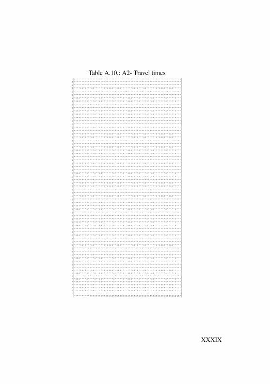
Table A.10.: A2- Travel timeso

i1i2

i3i4

i5i6

i7i8

i9i1

0i1

1i1

2i1

3i1

4i1

5i1

6i1

7i1

8i1

9i2

0i2

1i2

2i2

3i2

4i2

5i2

6i2

7i2

8i2

9i3

0i3

1i3

2i3

3i3

4i3

5i3

6i3

7i3

8i3

9i4

0i4

1i4

2i4

3i4

4i4

5i4

6i4

7i4

8i4

9i5

0i5

1i5

2i5

3i5

4i5

5i5

6i5

7i5

8i5

9i6

0i6

1i6

2i6

3i6

4i6

5i6

6o

o0

55

55

55

55

55

55

55

55

55

55

55

55

55

55

55

55

55

55

55

55

55

55

55

55

55

55

55

55

55

55

55

55

55

0i1

50

00

1010

510

05

510

100

55

00

510

510

1010

100

510

1010

50

55

00

010

105

100

55

1010

05

50

05

105

1010

1010

05

1010

105

05

55

i25

00

010

105

100

55

1010

05

50

05

105

1010

1010

05

1010

105

05

50

00

1010

510

05

510

100

55

00

510

510

1010

100

510

1010

50

55

5i3

50

00

1010

510

05

510

100

55

00

510

510

1010

100

510

1010

50

55

00

010

105

100

55

1010

05

50

05

105

1010

1010

05

1010

105

05

55

i45

1010

100

05

010

55

00

105

510

105

05

00

00

105

00

05

105

510

1010

00

50

105

50

010

55

1010

50

50

00

010

50

00

510

55

5i5

510

1010

00

50

105

50

010

55

1010

50

50

00

010

50

00

510

55

1010

100

05

010

55

00

105

510

105

05

00

00

105

00

05

105

55

i65

55

55

50

55

00

55

50

05

50

50

55

55

50

55

50

50

05

55

55

05

50

05

55

00

55

05

05

55

55

05

55

05

00

5i7

510

1010

00

50

105

50

010

55

1010

50

50

00

010

50

00

510

55

1010

100

05

010

55

00

105

510

105

05

00

00

105

00

05

105

55

i85

00

010

105

100

55

1010

05

50

05

105

1010

1010

05

1010

105

05

50

00

1010

510

05

510

100

55

00

510

510

1010

100

510

1010

50

55

5i9

55

55

55

05

50

05

55

00

55

05

05

55

55

05

55

05

00

55

55

50

55

00

55

50

05

50

50

55

55

50

55

50

50

05

i10

55

55

55

05

50

05

55

00

55

05

05

55

55

05

55

05

00

55

55

50

55

00

55

50

05

50

50

55

55

50

55

50

50

05

i11

510

1010

00

50

105

50

010

55

1010

50

50

00

010

50

00

510

55

1010

100

05

010

55

00

105

510

105

05

00

00

105

00

05

105

55

i12

510

1010

00

50

105

50

010

55

1010

50

50

00

010

50

00

510

55

1010

100

05

010

55

00

105

510

105

05

00

00

105

00

05

105

55

i13

50

00

1010

510

05

510

100

55

00

510

510

1010

100

510

1010

50

55

00

010

105

100

55

1010

05

50

05

105

1010

1010

05

1010

105

05

55

i14

55

55

55

05

50

05

55

00

55

05

05

55

55

05

55

05

00

55

55

50

55

00

55

50

05

50

50

55

55

50

55

50

50

05

i15

55

55

55

05

50

05

55

00

55

05

05

55

55

05

55

05

00

55

55

50

55

00

55

50

05

50

50

55

55

50

55

50

50

05

i16

50

00

1010

510

05

510

100

55

00

510

510

1010

100

510

1010

50

55

00

010

105

100

55

1010

05

50

05

105

1010

1010

05

1010

105

05

55

i17

50

00

1010

510

05

510

100

55

00

510

510

1010

100

510

1010

50

55

00

010

105

100

55

1010

05

50

05

105

1010

1010

05

1010

105

05

55

i18

55

55

55

05

50

05

55

00

55

05

05

55

55

05

55

05

00

55

55

50

55

00

55

50

05

50

50

55

55

50

55

50

50

05

i19

510

1010

00

50

105

50

010

55

1010

50

50

00

010

50

00

510

55

1010

100

05

010

55

00

105

510

105

05

00

00

105

00

05

105

55

i20

55

55

55

05

50

05

55

00

55

05

05

55

55

05

55

05

00

55

55

50

55

00

55

50

05

50

50

55

55

50

55

50

50

05

i21

510

1010

00

50

105

50

010

55

1010

50

50

00

010

50

00

510

55

1010

100

05

010

55

00

105

510

105

05

00

00

105

00

05

105

55

i22

510

1010

00

50

105

50

010

55

1010

50

50

00

010

50

00

510

55

1010

100

05

010

55

00

105

510

105

05

00

00

105

00

05

105

55

i23

510

1010

00

50

105

50

010

55

1010

50

50

00

010

50

00

510

55

1010

100

05

010

55

00

105

510

105

05

00

00

105

00

05

105

55

i24

510

1010

00

50

105

50

010

55

1010

50

50

00

010

50

00

510

55

1010

100

05

010

55

00

105

510

105

05

00

00

105

00

05

105

55

i25

50

00

1010

510

05

510

100

55

00

510

510

1010

100

510

1010

50

55

00

010

105

100

55

1010

05

50

05

105

1010

1010

05

1010

105

05

55

i26

55

55

55

05

50

05

55

00

55

05

05

55

55

05

55

05

00

55

55

50

55

00

55

50

05

50

50

55

55

50

55

50

50

05

i27

510

1010

00

50

105

50

010

55

1010

50

50

00

010

50

00

510

55

1010

100

05

010

55

00

105

510

105

05

00

00

105

00

05

105

55

i28

510

1010

00

50

105

50

010

55

1010

50

50

00

010

50

00

510

55

1010

100

05

010

55

00

105

510

105

05

00

00

105

00

05

105

55

i29

510

1010

00

50

105

50

010

55

1010

50

50

00

010

50

00

510

55

1010

100

05

010

55

00

105

510

105

05

00

00

105

00

05

105

55

i30

55

55

55

05

50

05

55

00

55

05

05

55

55

05

55

05

00

55

55

50

55

00

55

50

05

50

50

55

55

50

55

50

50

05

i31

50

00

1010

510

05

510

100

55

00

510

510

1010

100

510

1010

50

55

00

010

105

100

55

1010

05

50

05

105

1010

1010

05

1010

105

05

55

i32

55

55

55

05

50

05

55

00

55

05

05

55

55

05

55

05

00

55

55

50

55

00

55

50

05

50

50

55

55

50

55

50

50

05

i33

55

55

55

05

50

05

55

00

55

05

05

55

55

05

55

05

00

55

55

50

55

00

55

50

05

50

50

55

55

50

55

50

50

05

i34

50

00

1010

510

05

510

100

55

00

510

510

1010

100

510

1010

50

55

00

010

105

100

55

1010

05

50

05

105

1010

1010

05

1010

105

05

55

i35

50

00

1010

510

05

510

100

55

00

510

510

1010

100

510

1010

50

55

00

010

105

100

55

1010

05

50

05

105

1010

1010

05

1010

105

05

55

i36

50

00

1010

510

05

510

100

55

00

510

510

1010

100

510

1010

50

55

00

010

105

100

55

1010

05

50

05

105

1010

1010

05

1010

105

05

55

i37

510

1010

00

50

105

50

010

55

1010

50

50

00

010

50

00

510

55

1010

100

05

010

55

00

105

510

105

05

00

00

105

00

05

105

55

i38

510

1010

00

50

105

50

010

55

1010

50

50

00

010

50

00

510

55

1010

100

05

010

55

00

105

510

105

05

00

00

105

00

05

105

55

i39

55

55

55

05

50

05

55

00

55

05

05

55

55

05

55

05

00

55

55

50

55

00

55

50

05

50

50

55

55

50

55

50

50

05

i40

510

1010

00

50

105

50

010

55

1010

50

50

00

010

50

00

510

55

1010

100

05

010

55

00

105

510

105

05

00

00

105

00

05

105

55

i41

50

00

1010

510

05

510

100

55

00

510

510

1010

100

510

1010

50

55

00

010

105

100

55

1010

05

50

05

105

1010

1010

05

1010

105

05

55

i42

55

55

55

05

50

05

55

00

55

05

05

55

55

05

55

05

00

55

55

50

55

00

55

50

05

50

50

55

55

50

55

50

50

05

i43

55

55

55

05

50

05

55

00

55

05

05

55

55

05

55

05

00

55

55

50

55

00

55

50

05

50

50

55

55

50

55

50

50

05

i44

510

1010

00

50

105

50

010

55

1010

50

50

00

010

50

00

510

55

1010

100

05

010

55

00

105

510

105

05

00

00

105

00

05

105

55

i45

510

1010

00

50

105

50

010

55

1010

50

50

00

010

50

00

510

55

1010

100

05

010

55

00

105

510

105

05

00

00

105

00

05

105

55

i46

50

00

1010

510

05

510

100

55

00

510

510

1010

100

510

1010

50

55

00

010

105

100

55

1010

05

50

05

105

1010

1010

05

1010

105

05

55

i47

55

55

55

05

50

05

55

00

55

05

05

55

55

05

55

05

00

55

55

50

55

00

55

50

05

50

50

55

55

50

55

50

50

05

i48

55

55

55

05

50

05

55

00

55

05

05

55

55

05

55

05

00

55

55

50

55

00

55

50

05

50

50

55

55

50

55

50

50

05

i49

50

00

1010

510

05

510

100

55

00

510

510

1010

100

510

1010

50

55

00

010

105

100

55

1010

05

50

05

105

1010

1010

05

1010

105

05

55

i50

50

00

1010

510

05

510

100

55

00

510

510

1010

100

510

1010

50

55

00

010

105

100

55

1010

05

50

05

105

1010

1010

05

1010

105

05

55

i51

55

55

55

05

50

05

55

00

55

05

05

55

55

05

55

05

00

55

55

50

55

00

55

50

05

50

50

55

55

50

55

50

50

05

i52

510

1010

00

50

105

50

010

55

1010

50

50

00

010

50

00

510

55

1010

100

05

010

55

00

105

510

105

05

00

00

105

00

05

105

55

i53

55

55

55

05

50

05

55

00

55

05

05

55

55

05

55

05

00

55

55

50

55

00

55

50

05

50

50

55

55

50

55

50

50

05

i54

510

1010

00

50

105

50

010

55

1010

50

50

00

010

50

00

510

55

1010

100

05

010

55

00

105

510

105

05

00

00

105

00

05

105

55

i55

510

1010

00

50

105

50

010

55

1010

50

50

00

010

50

00

510

55

1010

100

05

010

55

00

105

510

105

05

00

00

105

00

05

105

55

i56

510

1010

00

50

105

50

010

55

1010

50

50

00

010

50

00

510

55

1010

100

05

010

55

00

105

510

105

05

00

00

105

00

05

105

55

i57

510

1010

00

50

105

50

010

55

1010

50

50

00

010

50

00

510

55

1010

100

05

010

55

00

105

510

105

05

00

00

105

00

05

105

55

i58

50

00

1010

510

05

510

100

55

00

510

510

1010

100

510

1010

50

55

00

010

105

100

55

1010

05

50

05

105

1010

1010

05

1010

105

05

55

i59

55

55

55

05

50

05

55

00

55

05

05

55

55

05

55

05

00

55

55

50

55

00

55

50

05

50

50

55

55

50

55

50

50

05

i60

510

1010

00

50

105

50

010

55

1010

50

50

00

010

50

00

510

55

1010

100

05

010

55

00

105

510

105

05

00

00

105

00

05

105

55

i61

510

1010

00

50

105

50

010

55

1010

50

50

00

010

50

00

510

55

1010

100

05

010

55

00

105

510

105

05

00

00

105

00

05

105

55

i62

510

1010

00

50

105

50

010

55

1010

50

50

00

010

50

00

510

55

1010

100

05

010

55

00

105

510

105

05

00

00

105

00

05

105

55

i63

55

55

55

05

50

05

55

00

55

05

05

55

55

05

55

05

00

55

55

50

55

00

55

50

05

50

50

55

55

50

55

50

50

05

i64

50

00

1010

510

05

510

100

55

00

510

510

1010

100

510

1010

50

55

00

010

105

100

55

1010

05

50

05

105

1010

1010

05

1010

105

05

55

i65

55

55

55

05

50

05

55

00

55

05

05

55

55

05

55

05

00

55

55

50

55

00

55

50

05

50

50

55

55

50

55

50

50

05

i66

55

55

55

05

50

05

55

00

55

05

05

55

55

05

55

05

00

55

55

50

55

00

55

50

05

50

50

55

55

50

55

50

50

05

o0

55

55

55

55

55

55

55

55

55

55

55

55

55

55

55

55

55

55

55

55

55

55

55

55

55

55

55

55

55

55

55

55

55

0

XXXIX

Table A.11.: A3- Travel times

oi1

i2i3

i4i5

i6i7

i8i9

i10

i11

i12

i13

i14

i15

i16

i17

i18

i19

i20

i21

i22

i23

i24

i25

i26

i27

i28

i29

i30

i31

i32

i33

i34

i35

i36

i37

i38

i39

i40

i41

i42

i43

i44

i45

i46

i47

i48

i49

i50

i51

i52

i53

i54

i55

i56

i57

i58

i59

i60

i61

i62

o

o0

55

55

55

55

55

55

55

55

55

55

55

55

55

55

55

55

55

55

55

55

55

55

55

55

55

55

55

55

55

55

55

0i1

50

1010

105

55

510

100

05

55

100

1010

1010

105

55

1010

100

55

010

1010

55

55

1010

00

55

510

010

1010

1010

55

510

1010

05

55

i25

100

00

55

55

00

1010

55

50

100

00

00

55

50

00

105

510

00

05

55

50

010

105

55

010

00

00

05

55

00

010

55

5i3

510

00

05

55

50

010

105

55

010

00

00

05

55

00

010

55

100

00

55

55

00

1010

55

50

100

00

00

55

50

00

105

55

i45

100

00

55

55

00

1010

55

50

100

00

00

55

50

00

105

510

00

05

55

50

010

105

55

010

00

00

05

55

00

010

55

5i5

55

55

50

00

05

55

50

00

55

55

55

50

00

55

55

00

55

55

00

00

55

55

00

05

55

55

55

00

05

55

50

05

i65

55

55

00

00

55

55

00

05

55

55

55

00

05

55

50

05

55

50

00

05

55

50

00

55

55

55

50

00

55

55

00

5i7

55

55

50

00

05

55

50

00

55

55

55

50

00

55

55

00

55

55

00

00

55

55

00

05

55

55

55

00

05

55

50

05

i85

55

55

00

00

55

55

00

05

55

55

55

00

05

55

50

05

55

50

00

05

55

50

00

55

55

55

50

00

55

55

00

5i9

510

00

05

55

50

010

105

55

010

00

00

05

55

00

010

55

100

00

55

55

00

1010

55

50

100

00

00

55

50

00

105

55

i10

510

00

05

55

50

010

105

55

010

00

00

05

55

00

010

55

100

00

55

55

00

1010

55

50

100

00

00

55

50

00

105

55

i11

50

1010

105

55

510

100

05

55

100

1010

1010

105

55

1010

100

55

010

1010

55

55

1010

00

55

510

010

1010

1010

55

510

1010

05

55

i12

50

1010

105

55

510

100

05

55

100

1010

1010

105

55

1010

100

55

010

1010

55

55

1010

00

55

510

010

1010

1010

55

510

1010

05

55

i13

55

55

50

00

05

55

50

00

55

55

55

50

00

55

55

00

55

55

00

00

55

55

00

05

55

55

55

00

05

55

50

05

i14

55

55

50

00

05

55

50

00

55

55

55

50

00

55

55

00

55

55

00

00

55

55

00

05

55

55

55

00

05

55

50

05

i15

55

55

50

00

05

55

50

00

55

55

55

50

00

55

55

00

55

55

00

00

55

55

00

05

55

55

55

00

05

55

50

05

i16

510

00

05

55

50

010

105

55

010

00

00

05

55

00

010

55

100

00

55

55

00

1010

55

50

100

00

00

55

50

00

105

55

i17

50

1010

105

55

510

100

05

55

100

1010

1010

105

55

1010

100

55

010

1010

55

55

1010

00

55

510

010

1010

1010

55

510

1010

05

55

i18

510

00

05

55

50

010

105

55

010

00

00

05

55

00

010

55

100

00

55

55

00

1010

55

50

100

00

00

55

50

00

105

55

i19

510

00

05

55

50

010

105

55

010

00

00

05

55

00

010

55

100

00

55

55

00

1010

55

50

100

00

00

55

50

00

105

55

i20

510

00

05

55

50

010

105

55

010

00

00

05

55

00

010

55

100

00

55

55

00

1010

55

50

100

00

00

55

50

00

105

55

i21

510

00

05

55

50

010

105

55

010

00

00

05

55

00

010

55

100

00

55

55

00

1010

55

50

100

00

00

55

50

00

105

55

i22

510

00

05

55

50

010

105

55

010

00

00

05

55

00

010

55

100

00

55

55

00

1010

55

50

100

00

00

55

50

00

105

55

i23

55

55

50

00

05

55

50

00

55

55

55

50

00

55

55

00

55

55

00

00

55

55

00

05

55

55

55

00

05

55

50

05

i24

55

55

50

00

05

55

50

00

55

55

55

50

00

55

55

00

55

55

00

00

55

55

00

05

55

55

55

00

05

55

50

05

i25

55

55

50

00

05

55

50

00

55

55

55

50

00

55

55

00

55

55

00

00

55

55

00

05

55

55

55

00

05

55

50

05

i26

510

00

05

55

50

010

105

55

010

00

00

05

55

00

010

55

100

00

55

55

00

1010

55

50

100

00

00

55

50

00

105

55

i27

510

00

05

55

50

010

105

55

010

00

00

05

55

00

010

55

100

00

55

55

00

1010

55

50

100

00

00

55

50

00

105

55

i28

510

00

05

55

50

010

105

55

010

00

00

05

55

00

010

55

100

00

55

55

00

1010

55

50

100

00

00

55

50

00

105

55

i29

50

1010

105

55

510

100

05

55

100

1010

1010

105

55

1010

100

55

010

1010

55

55

1010

00

55

510

010

1010

1010

55

510

1010

05

55

i30

55

55

50

00

05

55

50

00

55

55

55

50

00

55

55

00

55

55

00

00

55

55

00

05

55

55

55

00

05

55

50

05

i31

55

55

50

00

05

55

50

00

55

55

55

50

00

55

55

00

55

55

00

00

55

55

00

05

55

55

55

00

05

55

50

05

i32

50

1010

105

55

510

100

05

55

100

1010

1010

105

55

1010

100

55

010

1010

55

55

1010

00

55

510

010

1010

1010

55

510

1010

05

55

i33

510

00

05

55

50

010

105

55

010

00

00

05

55

00

010

55

100

00

55

55

00

1010

55

50

100

00

00

55

50

00

105

55

i34

510

00

05

55

50

010

105

55

010

00

00

05

55

00

010

55

100

00

55

55

00

1010

55

50

100

00

00

55

50

00

105

55

i35

510

00

05

55

50

010

105

55

010

00

00

05

55

00

010

55

100

00

55

55

00

1010

55

50

100

00

00

55

50

00

105

55

i36

55

55

50

00

05

55

50

00

55

55

55

50

00

55

55

00

55

55

00

00

55

55

00

05

55

55

55

00

05

55

50

05

i37

55

55

50

00

05

55

50

00

55

55

55

50

00

55

55

00

55

55

00

00

55

55

00

05

55

55

55

00

05

55

50

05

i38

55

55

50

00

05

55

50

00

55

55

55

50

00

55

55

00

55

55

00

00

55

55

00

05

55

55

55

00

05

55

50

05

i39

55

55

50

00

05

55

50

00

55

55

55

50

00

55

55

00

55

55

00

00

55

55

00

05

55

55

55

00

05

55

50

05

i40

510

00

05

55

50

010

105

55

010

00

00

05

55

00

010

55

100

00

55

55

00

1010

55

50

100

00

00

55

50

00

105

55

i41

510

00

05

55

50

010

105

55

010

00

00

05

55

00

010

55

100

00

55

55

00

1010

55

50

100

00

00

55

50

00

105

55

i42

50

1010

105

55

510

100

05

55

100

1010

1010

105

55

1010

100

55

010

1010

55

55

1010

00

55

510

010

1010

1010

55

510

1010

05

55

i43

50

1010

105

55

510

100

05

55

100

1010

1010

105

55

1010

100

55

010

1010

55

55

1010

00

55

510

010

1010

1010

55

510

1010

05

55

i44

55

55

50

00

05

55

50

00

55

55

55

50

00

55

55

00

55

55

00

00

55

55

00

05

55

55

55

00

05

55

50

05

i45

55

55

50

00

05

55

50

00

55

55

55

50

00

55

55

00

55

55

00

00

55

55

00

05

55

55

55

00

05

55

50

05

i46

55

55

50

00

05

55

50

00

55

55

55

50

00

55

55

00

55

55

00

00

55

55

00

05

55

55

55

00

05

55

50

05

i47

510

00

05

55

50

010

105

55

010

00

00

05

55

00

010

55

100

00

55

55

00

1010

55

50

100

00

00

55

50

00

105

55

i48

50

1010

105

55

510

100

05

55

100

1010

1010

105

55

1010

100

55

010

1010

55

55

1010

00

55

510

010

1010

1010

55

510

1010

05

55

i49

510

00

05

55

50

010

105

55

010

00

00

05

55

00

010

55

100

00

55

55

00

1010

55

50

100

00

00

55

50

00

105

55

i50

510

00

05

55

50

010

105

55

010

00

00

05

55

00

010

55

100

00

55

55

00

1010

55

50

100

00

00

55

50

00

105

55

i51

510

00

05

55

50

010

105

55

010

00

00

05

55

00

010

55

100

00

55

55

00

1010

55

50

100

00

00

55

50

00

105

55

i52

510

00

05

55

50

010

105

55

010

00

00

05

55

00

010

55

100

00

55

55

00

1010

55

50

100

00

00

55

50

00

105

55

i53

510

00

05

55

50

010

105

55

010

00

00

05

55

00

010

55

100

00

55

55

00

1010

55

50

100

00

00

55

50

00

105

55

i54

55

55

50

00

05

55

50

00

55

55

55

50

00

55

55

00

55

55

00

00

55

55

00

05

55

55

55

00

05

55

50

05

i55

55

55

50

00

05

55

50

00

55

55

55

50

00

55

55

00

55

55

00

00

55

55

00

05

55

55

55

00

05

55

50

05

i56

55

55

50

00

05

55

50

00

55

55

55

50

00

55

55

00

55

55

00

00

55

55

00

05

55

55

55

00

05

55

50

05

i57

510

00

05

55

50

010

105

55

010

00

00

05

55

00

010

55

100

00

55

55

00

1010

55

50

100

00

00

55

50

00

105

55

i58

510

00

05

55

50

010

105

55

010

00

00

05

55

00

010

55

100

00

55

55

00

1010

55

50

100

00

00

55

50

00

105

55

i59

510

00

05

55

50

010

105

55

010

00

00

05

55

00

010

55

100

00

55

55

00

1010

55

50

100

00

00

55

50

00

105

55

i60

50

1010

105

55

510

100

05

55

100

1010

1010

105

55

1010

100

55

010

1010

55

55

1010

00

55

510

010

1010

1010

55

510

1010

05

55

i61

55

55

50

00

05

55

50

00

55

55

55

50

00

55

55

00

55

55

00

00

55

55

00

05

55

55

55

00

05

55

50

05

i62

55

55

50

00

05

55

50

00

55

55

55

50

00

55

55

00

55

55

00

00

55

55

00

05

55

55

55

00

05

55

50

05

o0

55

55

55

55

55

55

55

55

55

55

55

55

55

55

55

55

55

55

55

55

55

55

55

55

55

55

55

55

55

55

55

0

XL

Table A.12.: A4- Travel timeso

i1i2

i3i4

i5i6

i7i8

i9i1

0i1

1i1

2i1

3i1

4i1

5i1

6i1

7i1

8i1

9i2

0i2

1i2

2i2

3i2

4i2

5i2

6i2

7i2

8i2

9i3

0i3

1i3

2i3

3i3

4i3

5i3

6i3

7i3

8i3

9i4

0i4

1i4

2i4

3i4

4i4

5i4

6i4

7i4

8i4

9i5

0o

o0

55

55

55

55

55

55

55

55

55

55

55

55

55

55

55

55

55

55

55

55

55

55

55

55

55

0i1

50

510

1010

55

010

100

55

105

1010

05

1010

100

55

05

1010

105

50

1010

05

510

510

100

510

1010

05

55

i25

50

55

50

05

55

50

05

05

55

05

55

50

05

05

55

00

55

55

00

50

55

50

55

55

00

5i3

510

50

00

55

100

010

55

05

00

105

00

010

55

105

00

05

510

00

105

50

50

010

50

00

105

55

i45

105

00

05

510

00

105

50

50

010

50

00

105

510

50

00

55

100

010

55

05

00

105

00

010

55

5i5

510

50

00

55

100

010

55

05

00

105

00

010

55

105

00

05

510

00

105

50

50

010

50

00

105

55

i65

50

55

50

05

55

50

05

05

55

05

55

50

05

05

55

00

55

55

00

50

55

50

55

55

00

5i7

55

05

55

00

55

55

00

50

55

50

55

55

00

50

55

50

05

55

50

05

05

55

05

55

50

05

i85

05

1010

105

50

1010

05

510

510

100

510

1010

05

50

510

1010

55

010

100

55

105

1010

05

1010

100

55

5i9

510

50

00

55

100

010

55

05

00

105

00

010

55

105

00

05

510

00

105

50

50

010

50

00

105

55

i10

510

50

00

55

100

010

55

05

00

105

00

010

55

105

00

05

510

00

105

50

50

010

50

00

105

55

i11

50

510

1010

55

010

100

55

105

1010

05

1010

100

55

05

1010

105

50

1010

05

510

510

100

510

1010

05

55

i12

55

05

55

00

55

55

00

50

55

50

55

55

00

50

55

50

05

55

50

05

05

55

05

55

50

05

i13

55

05

55

00

55

55

00

50

55

50

55

55

00

50

55

50

05

55

50

05

05

55

05

55

50

05

i14

510

50

00

55

100

010

55

05

00

105

00

010

55

105

00

05

510

00

105

50

50

010

50

00

105

55

i15

55

05

55

00

55

55

00

50

55

50

55

55

00

50

55

50

05

55

50

05

05

55

05

55

50

05

i16

510

50

00

55

100

010

55

05

00

105

00

010

55

105

00

05

510

00

105

50

50

010

50

00

105

55

i17

510

50

00

55

100

010

55

05

00

105

00

010

55

105

00

05

510

00

105

50

50

010

50

00

105

55

i18

50

510

1010

55

010

100

55

105

1010

05

1010

100

55

05

1010

105

50

1010

05

510

510

100

510

1010

05

55

i19

55

05

55

00

55

55

00

50

55

50

55

55

00

50

55

50

05

55

50

05

05

55

05

55

50

05

i20

510

50

00

55

100

010

55

05

00

105

00

010

55

105

00

05

510

00

105

50

50

010

50

00

105

55

i21

510

50

00

55

100

010

55

05

00

105

00

010

55

105

00

05

510

00

105

50

50

010

50

00

105

55

i22

510

50

00

55

100

010

55

05

00

105

00

010

55

105

00

05

510

00

105

50

50

010

50

00

105

55

i23

50

510

1010

55

010

100

55

105

1010

05

1010

100

55

05

1010

105

50

1010

05

510

510

100

510

1010

05

55

i24

55

05

55

00

55

55

00

50

55

50

55

55

00

50

55

50

05

55

50

05

05

55

05

55

50

05

i25

55

05

55

00

55

55

00

50

55

50

55

55

00

50

55

50

05

55

50

05

05

55

05

55

50

05

i26

50

510

1010

55

010

100

55

105

1010

05

1010

100

55

05

1010

105

50

1010

05

510

510

100

510

1010

05

55

i27

55

05

55

00

55

55

00

50

55

50

55

55

00

50

55

50

05

55

50

05

05

55

05

55

50

05

i28

510

50

00

55

100

010

55

05

00

105

00

010

55

105

00

05

510

00

105

50

50

010

50

00

105

55

i29

510

50

00

55

100

010

55

05

00

105

00

010

55

105

00

05

510

00

105

50

50

010

50

00

105

55

i30

510

50

00

55

100

010

55

05

00

105

00

010

55

105

00

05

510

00

105

50

50

010

50

00

105

55

i31

55

05

55

00

55

55

00

50

55

50

55

55

00

50

55

50

05

55

50

05

05

55

05

55

50

05

i32

55

05

55

00

55

55

00

50

55

50

55

55

00

50

55

50

05

55

50

05

05

55

05

55

50

05

i33

50

510

1010

55

010

100

55

105

1010

05

1010

100

55

05

1010

105

50

1010

05

510

510

100

510

1010

05

55

i34

510

50

00

55

100

010

55

05

00

105

00

010

55

105

00

05

510

00

105

50

50

010

50

00

105

55

i35

510

50

00

55

100

010

55

05

00

105

00

010

55

105

00

05

510

00

105

50

50

010

50

00

105

55

i36

50

510

1010

55

010

100

55

105

1010

05

1010

100

55

05

1010

105

50

1010

05

510

510

100

510

1010

05

55

i37

55

05

55

00

55

55

00

50

55

50

55

55

00

50

55

50

05

55

50

05

05

55

05

55

50

05

i38

55

05

55

00

55

55

00

50

55

50

55

55

00

50

55

50

05

55

50

05

05

55

05

55

50

05

i39

510

50

00

55

100

010

55

05

00

105

00

010

55

105

00

05

510

00

105

50

50

010

50

00

105

55

i40

55

05

55

00

55

55

00

50

55

50

55

55

00

50

55

50

05

55

50

05

05

55

05

55

50

05

i41

510

50

00

55

100

010

55

05

00

105

00

010

55

105

00

05

510

00

105

50

50

010

50

00

105

55

i42

510

50

00

55

100

010

55

05

00

105

00

010

55

105

00

05

510

00

105

50

50

010

50

00

105

55

i43

50

510

1010

55

010

100

55

105

1010

05

1010

100

55

05

1010

105

50

1010

05

510

510

100

510

1010

05

55

i44

55

05

55

00

55

55

00

50

55

50

55

55

00

50

55

50

05

55

50

05

05

55

05

55

50

05

i45

510

50

00

55

100

010

55

05

00

105

00

010

55

105

00

05

510

00

105

50

50

010

50

00

105

55

i46

510

50

00

55

100

010

55

05

00

105

00

010

55

105

00

05

510

00

105

50

50

010

50

00

105

55

i47

510

50

00

55

100

010

55

05

00

105

00

010

55

105

00

05

510

00

105

50

50

010

50

00

105

55

i48

50

510

1010

55

010

100

55

105

1010

05

1010

100

55

05

1010

105

50

1010

05

510

510

100

510

1010

05

55

i49

55

05

55

00

55

55

00

50

55

50

55

55

00

50

55

50

05

55

50

05

05

55

05

55

50

05

i50

55

05

55

00

55

55

00

50

55

50

55

55

00

50

55

50

05

55

50

05

05

55

05

55

50

05

o0

55

55

55

55

55

55

55

55

55

55

55

55

55

55

55

55

55

55

55

55

55

55

55

55

55

0

XLI

B. Results for realistic instances from Chapter4

The following section presents detailed results for instances A1-A4. TablesB.1 to B.4 show, for each agent, the overall overtime (in minutes) and theassigned route (starting and ending at the depot). Tables B.5 to B.8 presentthe starting time and overall waiting time (in minutes) per agent per task inthe final schedule.

XLIII

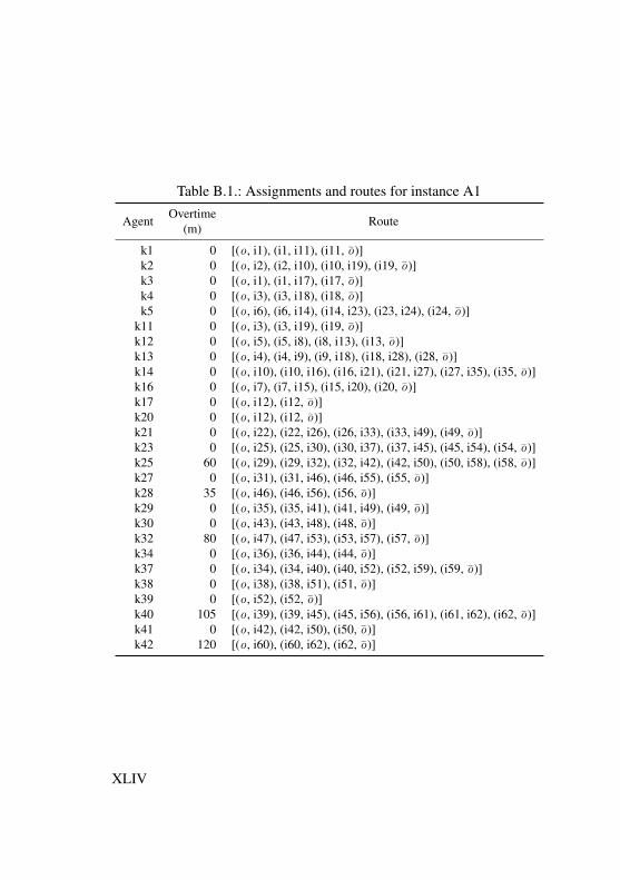
Table B.1.: Assignments and routes for instance A1

Agent Overtime Route(m)

k1 0 [(o, i1), (i1, i11), (i11, o)]k2 0 [(o, i2), (i2, i10), (i10, i19), (i19, o)]k3 0 [(o, i1), (i1, i17), (i17, o)]k4 0 [(o, i3), (i3, i18), (i18, o)]k5 0 [(o, i6), (i6, i14), (i14, i23), (i23, i24), (i24, o)]

k11 0 [(o, i3), (i3, i19), (i19, o)]k12 0 [(o, i5), (i5, i8), (i8, i13), (i13, o)]k13 0 [(o, i4), (i4, i9), (i9, i18), (i18, i28), (i28, o)]k14 0 [(o, i10), (i10, i16), (i16, i21), (i21, i27), (i27, i35), (i35, o)]k16 0 [(o, i7), (i7, i15), (i15, i20), (i20, o)]k17 0 [(o, i12), (i12, o)]k20 0 [(o, i12), (i12, o)]k21 0 [(o, i22), (i22, i26), (i26, i33), (i33, i49), (i49, o)]k23 0 [(o, i25), (i25, i30), (i30, i37), (i37, i45), (i45, i54), (i54, o)]k25 60 [(o, i29), (i29, i32), (i32, i42), (i42, i50), (i50, i58), (i58, o)]k27 0 [(o, i31), (i31, i46), (i46, i55), (i55, o)]k28 35 [(o, i46), (i46, i56), (i56, o)]k29 0 [(o, i35), (i35, i41), (i41, i49), (i49, o)]k30 0 [(o, i43), (i43, i48), (i48, o)]k32 80 [(o, i47), (i47, i53), (i53, i57), (i57, o)]k34 0 [(o, i36), (i36, i44), (i44, o)]k37 0 [(o, i34), (i34, i40), (i40, i52), (i52, i59), (i59, o)]k38 0 [(o, i38), (i38, i51), (i51, o)]k39 0 [(o, i52), (i52, o)]k40 105 [(o, i39), (i39, i45), (i45, i56), (i56, i61), (i61, i62), (i62, o)]k41 0 [(o, i42), (i42, i50), (i50, o)]k42 120 [(o, i60), (i60, i62), (i62, o)]

XLIV

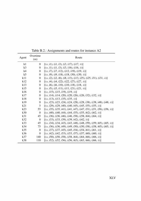
Table B.2.: Assignments and routes for instance A2

Agent Overtime Route(m)

k1 0 [(o, i1), (i1, i3), (i3, i17), (i17, o)]k3 0 [(o, i1), (i1, i3), (i3, i16), (i16, o)]k4 0 [(o, i7), (i7, i12), (i12, i19), (i19, o)]k5 0 [(o, i9), (i9, i18), (i18, i30), (i30, o)]

k11 0 [(o, i2), (i2, i8), (i8, i13), (i13, i25), (i25, i31), (i31, o)]k12 0 [(o, i4), (i4, i22), (i22, i27), (i27, o)]k13 0 [(o, i6), (i6, i10), (i10, i18), (i18, o)]k15 0 [(o, i5), (i5, i11), (i11, i21), (i21, o)]k16 0 [(o, i15), (i15, i19), (i19, o)]k17 0 [(o, i14), (i14, i20), (i20, i26), (i26, i32), (i32, o)]k18 0 [(o, i13), (i13, i35), (i35, o)]k19 0 [(o, i23), (i23, i24), (i24, i28), (i28, i38), (i38, i48), (i48, o)]k21 5 [(o, i29), (i29, i40), (i40, i45), (i45, i55), (i55, o)]k23 55 [(o, i35), (i35, i41), (i41, i47), (i47, i51), (i51, i56), (i56, o)]k30 0 [(o, i40), (i40, i44), (i44, i55), (i55, i62), (i62, o)]k31 45 [(o, i36), (i36, i46), (i46, i58), (i58, i64), (i64, o)]k32 0 [(o, i33), (i33, i39), (i39, i42), (i42, o)]k33 45 [(o, i34), (i34, i43), (i43, i48), (i48, i59), (i59, i65), (i65, o)]k34 75 [(o, i36), (i36, i49), (i49, i50), (i50, i58), (i58, i65), (i65, o)]k35 0 [(o, i37), (i37, i45), (i45, i54), (i54, i61), (i61, o)]k36 0 [(o, i42), (i42, i53), (i53, i57), (i57, i60), (i60, o)]k37 140 [(o, i50), (i50, i58), (i58, i64), (i64, i66), (i66, o)]k38 110 [(o, i52), (i52, i56), (i56, i63), (i63, i66), (i66, o)]

XLV

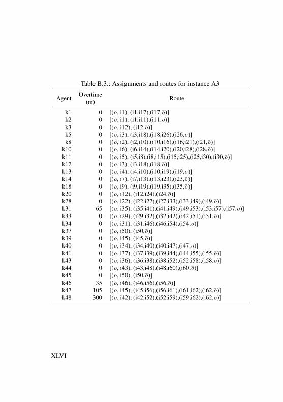
Table B.3.: Assignments and routes for instance A3

Agent Overtime Route(m)

k1 0 [(o, i1), (i1,i17),(i17,o)]k2 0 [(o, i1), (i1,i11),(i11,o)]k3 0 [(o, i12), (i12,o)]k5 0 [(o, i3), (i3,i18),(i18,i26),(i26,o)]k8 0 [(o, i2), (i2,i10),(i10,i16),(i16,i21),(i21,o)]

k10 0 [(o, i6), (i6,i14),(i14,i20),(i20,i28),(i28,o)]k11 0 [(o, i5), (i5,i8),(i8,i15),(i15,i25),(i25,i30),(i30,o)]k12 0 [(o, i3), (i3,i18),(i18,o)]k13 0 [(o, i4), (i4,i10),(i10,i19),(i19,o)]k14 0 [(o, i7), (i7,i13),(i13,i23),(i23,o)]k18 0 [(o, i9), (i9,i19),(i19,i35),(i35,o)]k20 0 [(o, i12), (i12,i24),(i24,o)]k28 0 [(o, i22), (i22,i27),(i27,i33),(i33,i49),(i49,o)]k31 65 [(o, i35), (i35,i41),(i41,i49),(i49,i53),(i53,i57),(i57,o)]k33 0 [(o, i29), (i29,i32),(i32,i42),(i42,i51),(i51,o)]k34 0 [(o, i31), (i31,i46),(i46,i54),(i54,o)]k37 0 [(o, i50), (i50,o)]k39 0 [(o, i45), (i45,o)]k40 0 [(o, i34), (i34,i40),(i40,i47),(i47,o)]k41 0 [(o, i37), (i37,i39),(i39,i44),(i44,i55),(i55,o)]k43 0 [(o, i36), (i36,i38),(i38,i52),(i52,i58),(i58,o)]k44 0 [(o, i43), (i43,i48),(i48,i60),(i60,o)]k45 0 [(o, i50), (i50,o)]k46 35 [(o, i46), (i46,i56),(i56,o)]k47 105 [(o, i45), (i45,i56),(i56,i61),(i61,i62),(i62,o)]k48 300 [(o, i42), (i42,i52),(i52,i59),(i59,i62),(i62,o)]

XLVI

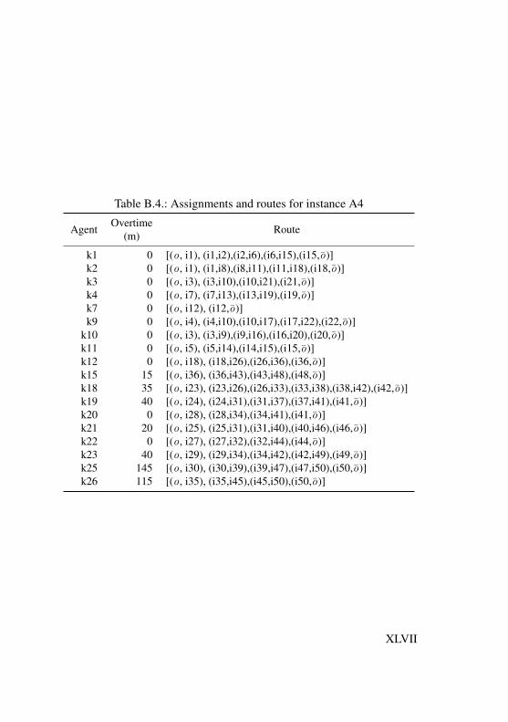
Table B.4.: Assignments and routes for instance A4

Agent Overtime Route(m)

k1 0 [(o, i1), (i1,i2),(i2,i6),(i6,i15),(i15,o)]k2 0 [(o, i1), (i1,i8),(i8,i11),(i11,i18),(i18,o)]k3 0 [(o, i3), (i3,i10),(i10,i21),(i21,o)]k4 0 [(o, i7), (i7,i13),(i13,i19),(i19,o)]k7 0 [(o, i12), (i12,o)]k9 0 [(o, i4), (i4,i10),(i10,i17),(i17,i22),(i22,o)]

k10 0 [(o, i3), (i3,i9),(i9,i16),(i16,i20),(i20,o)]k11 0 [(o, i5), (i5,i14),(i14,i15),(i15,o)]k12 0 [(o, i18), (i18,i26),(i26,i36),(i36,o)]k15 15 [(o, i36), (i36,i43),(i43,i48),(i48,o)]k18 35 [(o, i23), (i23,i26),(i26,i33),(i33,i38),(i38,i42),(i42,o)]k19 40 [(o, i24), (i24,i31),(i31,i37),(i37,i41),(i41,o)]k20 0 [(o, i28), (i28,i34),(i34,i41),(i41,o)]k21 20 [(o, i25), (i25,i31),(i31,i40),(i40,i46),(i46,o)]k22 0 [(o, i27), (i27,i32),(i32,i44),(i44,o)]k23 40 [(o, i29), (i29,i34),(i34,i42),(i42,i49),(i49,o)]k25 145 [(o, i30), (i30,i39),(i39,i47),(i47,i50),(i50,o)]k26 115 [(o, i35), (i35,i45),(i45,i50),(i50,o)]

XLVII

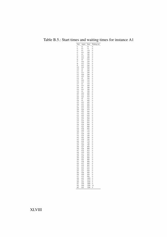
Table B.5.: Start times and waiting times for instance A1Task Agent Start Waiting (m)

i1 k1 75 0i1 k3 75 0i2 k2 170 0i3 k11 180 0i3 k4 180 0i4 k13 180 0i5 k12 200 0i6 k5 210 0i7 k16 220 0i8 k12 230 0i9 k13 240 0i10 k14 250 0i10 k2 250 0i11 k1 290 0i12 k17 290 0i12 k20 290 0i13 k12 290 0i14 k5 300 0i15 k16 310 0i16 k14 310 0i17 k3 310 0i18 k13 360 0i18 k4 360 0i19 k11 390 0i19 k2 390 0i20 k16 400 0i21 k14 405 0i22 k21 415 0i23 k5 415 0i24 k5 495 0i25 k23 495 0i26 k21 505 0i27 k14 505 0i28 k13 525 0i29 k25 575 0i30 k23 585 0i31 k27 585 0i32 k25 630 0i33 k21 635 0i34 k37 655 0i35 k14 655 0i35 k29 655 0i36 k34 660 0i37 k23 680 0i38 k38 695 0i39 k40 725 0i40 k37 735 0i41 k29 760 0i42 k25 760 0i42 k41 760 0i43 k30 765 0i44 k34 770 0i45 k23 780 0i45 k40 780 0i46 k27 800 0i46 k28 800 0i47 k32 815 0i48 k30 825 0i49 k21 845 0i49 k29 845 0i50 k25 880 0i50 k41 880 0i51 k38 880 0i52 k37 885 0i52 k39 885 0i53 k32 915 0i54 k23 925 0i55 k27 930 0i56 k28 950 0i56 k40 950 0i57 k32 990 0i58 k25 1005 0i59 k37 1015 0i60 k42 1020 0i61 k40 1080 0i62 k40 1200 15i62 k42 1200 0

XLVIII

Table B.6.: Start times and waiting times for instance A2Task Agent Start Waiting (m)

i1 k1 75 0i1 k3 75 0i2 k11 170 0i3 k1 180 0i3 k3 180 0i4 k12 180 0i5 k15 200 0i6 k13 200 0i7 k4 210 0i8 k11 220 0i9 k5 240 0i10 k13 275 0i11 k15 280 0i12 k4 290 0i13 k11 290 0i13 k18 290 0i14 k17 290 0i15 k16 300 0i16 k3 310 0i17 k1 310 0i18 k13 360 0i18 k5 360 0i19 k16 395 0i19 k4 395 0i20 k17 400 0i21 k15 405 0i22 k12 415 0i23 k19 415 0i24 k19 490 0i25 k11 495 0i26 k17 505 0i27 k12 505 0i28 k19 575 0i29 k21 585 0i30 k5 595 0i31 k11 600 0i32 k17 605 0i33 k32 630 0i34 k33 655 0i35 k18 655 0i35 k23 655 0i36 k31 695 0i36 k34 695 0i37 k35 695 0i38 k19 705 0i39 k32 725 0i40 k21 730 0i40 k30 730 0i41 k23 735 0i42 k32 760 0i42 k36 760 0i43 k33 765 0i44 k30 770 0i45 k21 810 0i45 k35 810 0i46 k31 815 0i47 k23 825 0i48 k19 830 0i48 k33 830 0i49 k34 835 0i50 k34 885 0i50 k37 885 0i51 k23 915 0i52 k38 915 0i53 k36 925 0i54 k35 930 0i55 k21 935 0i55 k30 935 0i56 k23 955 0i56 k38 955 0i57 k36 985 0i58 k31 1005 0i58 k34 1005 0i58 k37 1005 0i59 k33 1005 0i60 k36 1015 0i61 k35 1020 0i62 k30 1050 0i63 k38 1080 10i64 k31 1105 10i64 k37 1105 0i65 k33 1170 45i65 k34 1170 15i66 k38 1190 0i66 k37 1230 40

XLIX

Table B.7.: Start times and waiting times for instance A3Task Agent Start Waiting (m)

i1 k1 75 0i1 k2 75 0i2 k8 170 0i3 k12 180 0i3 k5 180 0i4 k13 180 0i5 k11 200 0i6 k10 210 0i7 k14 220 0i8 k11 230 0i9 k18 240 0i10 k13 250 0i10 k8 250 0i11 k2 290 0i12 k20 290 0i12 k3 290 0i13 k14 290 0i14 k10 300 0i15 k11 310 0i16 k8 310 0i17 k1 310 0i18 k12 360 0i18 k5 360 0i19 k13 390 0i19 k18 390 0i20 k10 400 0i21 k8 405 0i22 k28 415 0i23 k14 415 0i24 k20 495 0i25 k11 495 0i26 k5 505 0i27 k28 505 0i28 k10 525 0i29 k33 575 0i30 k11 585 0i31 k34 585 0i32 k33 630 0i33 k28 635 0i34 k40 655 0i35 k18 655 0i35 k31 655 0i36 k43 660 0i37 k41 680 0i38 k43 695 0i39 k41 725 0i40 k40 735 0i41 k31 760 0i42 k33 760 0i42 k48 760 0i43 k44 765 0i44 k41 770 0i45 k39 780 0i45 k47 780 0i46 k34 800 0i46 k46 800 0i47 k40 815 0i48 k44 825 0i49 k28 845 0i49 k31 845 0i50 k37 880 0i50 k45 880 0i51 k33 880 0i52 k43 885 0i52 k48 885 0i53 k31 915 0i54 k34 925 0i55 k41 930 0i56 k46 950 0i56 k47 950 0i57 k31 990 0i58 k43 1005 0i59 k48 1015 0i60 k44 1020 0i61 k47 1080 0i62 k47 1200 15i62 k48 1200 0i62 k30 1050 0i63 k38 1080 10i64 k31 1105 10i64 k37 1105 0i65 k33 1170 45i65 k34 1170 15i66 k38 1190 0i66 k37 1230 40

L

Table B.8.: Start times and waiting times for instance A4Task Agent Start Waiting (m)

i1 k1 75 0i1 k2 75 0i2 k1 170 0i3 k10 180 0i3 k3 180 0i4 k9 180 0i5 k11 200 0i6 k1 210 0i7 k4 220 0i8 k2 240 0i9 k10 290 0i10 k3 290 0i10 k9 290 0i11 k2 290 0i12 k7 300 0i13 k4 310 0i14 k11 350 0i15 k1 360 0i15 k11 385 25i16 k10 405 0i17 k9 415 0i18 k12 470 0i18 k2 470 0i19 k4 490 0i20 k10 495 0i21 k3 505 0i22 k9 575 0i23 k18 575 0i24 k19 600 0i25 k21 655 0i26 k12 655 0i26 k18 655 0i27 k22 685 0i28 k20 700 0i29 k23 725 0i30 k25 735 0i31 k19 760 0i31 k21 760 0i32 k22 815 0i33 k18 820 0i34 k20 820 0i34 k23 820 0i35 k26 825 0i36 k12 845 0i36 k15 845 0i37 k19 895 0i38 k18 915 0i39 k25 925 0i40 k21 930 0i41 k19 940 0i41 k20 940 0i42 k18 950 0i42 k23 950 0i43 k15 970 0i44 k22 975 0i45 k26 1005 0i46 k21 1005 0i47 k25 1015 0i48 k15 1020 0i49 k23 1060 5i50 k25 1110 20i50 k26 1100 10

LI

C. Results for instances with different shiftlength from Chapter 4

Table C.1.: Results with � = 0.7

Instance MIP BPObjective Abs. Gap (%) CPU (m) Objective CPU (m) Nodes Columns

1 243.60 0.00 60.00 243.60 3.65 34 10832 343.50 5.56 60.00 325.40 5.11 87 66083 INFEASIBLE4 346.20 0.00 13.91 346.20 1.62 75 9885 291.60 0.00 52.44 291.60 4.98 83 49866 261.90 0.00 10.46 261.90 1.38 30 9377 INFEASIBLE8 381.30 0.00 24.13 381.30 2.97 40 10939 375.90 0.00 12.03 375.90 5.22 80 8343

10 530.90 0.00 59.08 530.90 12.89 81 221111 334.20 0.00 2.78 334.20 1.20 47 81512 354.90 0.00 19.11 354.90 3.63 56 146813 318.20 0.00 3.56 318.20 3.04 107 1054014 182.60 0.00 46.41 182.60 2.80 34 122715 423.90 0.00 60.00 423.90 6.71 109 1294616 255.50 0.00 18.04 255.50 5.52 58 671117 378.40 0.00 7.69 378.40 1.41 46 90718 350.40 0.00 19.29 350.40 3.52 48 122719 458.40 0.00 33.74 458.40 6.53 88 1435820 552.40 0.00 31.62 552.40 10.45 67 204821 345.60 0.00 3.17 345.60 1.51 63 93622 369.90 0.00 26.14 369.90 5.03 81 166123 440.00 0.00 31.49 440.00 3.06 43 230624 436.10 0.00 18.34 436.10 7.21 87 17557

Average 362.52 0.25 27.88 361.70 4.52 65.64 4588.91

LIII

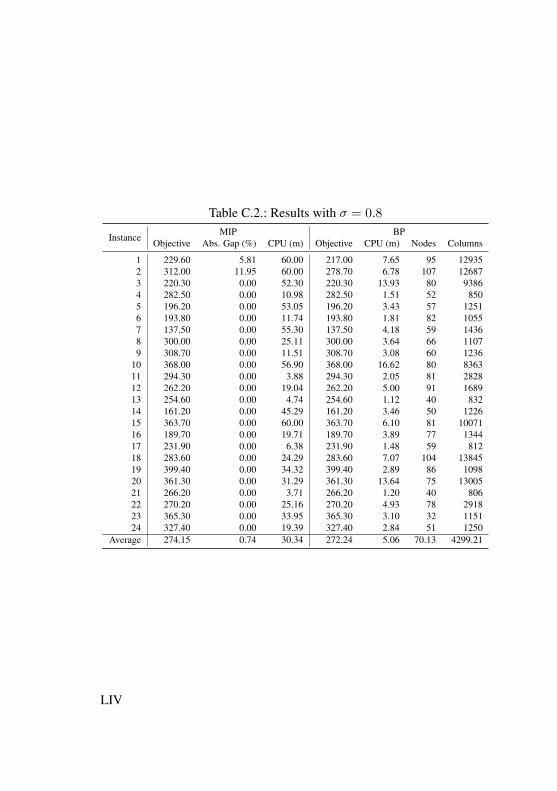
Table C.2.: Results with � = 0.8

Instance MIP BPObjective Abs. Gap (%) CPU (m) Objective CPU (m) Nodes Columns

1 229.60 5.81 60.00 217.00 7.65 95 129352 312.00 11.95 60.00 278.70 6.78 107 126873 220.30 0.00 52.30 220.30 13.93 80 93864 282.50 0.00 10.98 282.50 1.51 52 8505 196.20 0.00 53.05 196.20 3.43 57 12516 193.80 0.00 11.74 193.80 1.81 82 10557 137.50 0.00 55.30 137.50 4.18 59 14368 300.00 0.00 25.11 300.00 3.64 66 11079 308.70 0.00 11.51 308.70 3.08 60 1236

10 368.00 0.00 56.90 368.00 16.62 80 836311 294.30 0.00 3.88 294.30 2.05 81 282812 262.20 0.00 19.04 262.20 5.00 91 168913 254.60 0.00 4.74 254.60 1.12 40 83214 161.20 0.00 45.29 161.20 3.46 50 122615 363.70 0.00 60.00 363.70 6.10 81 1007116 189.70 0.00 19.71 189.70 3.89 77 134417 231.90 0.00 6.38 231.90 1.48 59 81218 283.60 0.00 24.29 283.60 7.07 104 1384519 399.40 0.00 34.32 399.40 2.89 86 109820 361.30 0.00 31.29 361.30 13.64 75 1300521 266.20 0.00 3.71 266.20 1.20 40 80622 270.20 0.00 25.16 270.20 4.93 78 291823 365.30 0.00 33.95 365.30 3.10 32 115124 327.40 0.00 19.39 327.40 2.84 51 1250

Average 274.15 0.74 30.34 272.24 5.06 70.13 4299.21

LIV

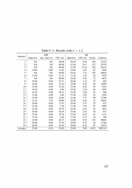
Table C.3.: Results with � = 1.2

Instance MIP BPObjective Abs. Gap (%) CPU (m) Objective CPU (m) Nodes Columns

1 NA NA 60.00 30.40 8.26 100 231542 NA NA 60.00 21.80 8.11 112 253703 NA NA 60.00 27.00 17.16 102 242744 19.60 0.00 11.65 19.60 2.01 62 76565 NA NA 60.00 24.20 7.33 105 200256 17.40 0.00 13.21 17.40 1.36 40 35387 NA NA 60.00 24.20 5.01 72 66578 30.40 0.00 23.71 30.40 2.12 35 8639 22.00 0.00 12.34 22.00 5.49 94 13095

10 27.00 0.00 57.62 27.00 8.29 50 232411 19.20 0.00 4.40 19.20 2.24 66 550312 24.20 0.00 20.14 24.20 2.84 53 96813 17.40 0.00 2.04 17.40 1.03 25 124214 23.40 0.00 43.86 23.40 7.77 98 1719615 31.45 3.45 60.00 30.40 6.38 72 1886116 20.80 0.00 17.81 20.80 2.27 25 82717 17.40 0.00 7.36 17.40 1.92 47 598918 23.40 0.00 20.72 23.40 2.24 54 182219 30.40 0.00 36.39 30.40 2.43 38 91720 27.60 0.00 32.24 27.60 6.22 42 113121 17.40 0.00 1.04 17.40 0.73 18 59922 24.00 0.00 26.47 24.00 9.35 135 3066223 30.80 0.00 32.19 30.80 4.35 50 1138424 20.80 0.00 16.39 20.80 6.30 87 12425

Average 23.40 0.18 30.82 23.80 5.05 65.92 9853.42

LV

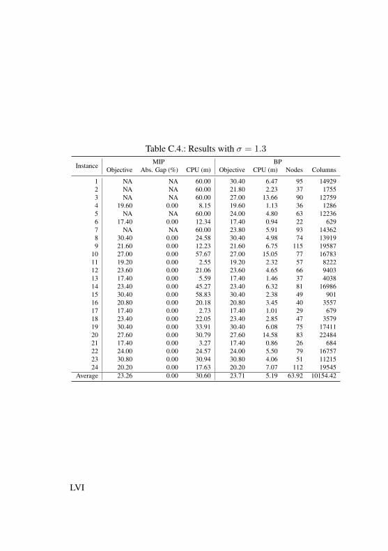
Table C.4.: Results with � = 1.3

Instance MIP BPObjective Abs. Gap (%) CPU (m) Objective CPU (m) Nodes Columns

1 NA NA 60.00 30.40 6.47 95 149292 NA NA 60.00 21.80 2.23 37 17553 NA NA 60.00 27.00 13.66 90 127594 19.60 0.00 8.15 19.60 1.13 36 12865 NA NA 60.00 24.00 4.80 63 122366 17.40 0.00 12.34 17.40 0.94 22 6297 NA NA 60.00 23.80 5.91 93 143628 30.40 0.00 24.58 30.40 4.98 74 139199 21.60 0.00 12.23 21.60 6.75 115 19587

10 27.00 0.00 57.67 27.00 15.05 77 1678311 19.20 0.00 2.55 19.20 2.32 57 822212 23.60 0.00 21.06 23.60 4.65 66 940313 17.40 0.00 5.59 17.40 1.46 37 403814 23.40 0.00 45.27 23.40 6.32 81 1698615 30.40 0.00 58.83 30.40 2.38 49 90116 20.80 0.00 20.18 20.80 3.45 40 355717 17.40 0.00 2.73 17.40 1.01 29 67918 23.40 0.00 22.05 23.40 2.85 47 357919 30.40 0.00 33.91 30.40 6.08 75 1741120 27.60 0.00 30.79 27.60 14.58 83 2248421 17.40 0.00 3.27 17.40 0.86 26 68422 24.00 0.00 24.57 24.00 5.50 79 1675723 30.80 0.00 30.94 30.80 4.06 51 1121524 20.20 0.00 17.63 20.20 7.07 112 19545

Average 23.26 0.00 30.60 23.71 5.19 63.92 10154.42

LVI

Curriculum Vitae

Emilio Zamorano de Acha

Personal Information

Place of birth Guadalajara, MexicoNationality German - Mexican

Education

2010—2016 Doctoral CandidateBusiness School, University of Mannheim

2008—2009 Master of Engineering (M. I.)Universidad Panamericana, Mexico

2003—2007 Industrial Engineering (B.Sc.)Universidad Panamericana, Mexico

Professional Experience

2011—2015 Research Assistant, Chair of Production Management,Business School, University of Mannheim

2008—2010 Industrial Engineering Program CoordinatorUniversidad Panamericana, Guadalajara, Mexico

2007—2008 Material Planning and Logistics TraineeFord Motor Co., Almussafes, Spain

LVIII