Title Variations of Structured Broyden Families for Nonlinear LeastSquares Problems

Author(s) Yabe, Hiroshi

Citation 数理解析研究所講究録 (1991), 746: 156-165

Issue Date 1991-03

URL http://hdl.handle.net/2433/102216

Right

Type Departmental Bulletin Paper

Textversion publisher

Kyoto University

156

Variations of Structured Broyden Families for Nonlinear LeastSquares Problems

東京理科大学・工学部 矢部 博 (Hiroshi Yabe)

1 Introduction

In this paper, we consider methods for finding a local solution, $x^{*}$ say, to a nonlinear leastsquares problem

(1) minimize $f(x)= \frac{1}{2}\sum_{j=1}^{m}(r_{j}(x))^{2}$ ,

where $r_{j}$ : $R^{n}arrow R,$ $j=1,$ $\ldots,$$m(m\geq n)$ are twice continuously differentiable. Such problems

arise widely in data fitting and in the solution of well-determined and over-determined systemsof equations. Among many numerical methods, structured quasi-Newton methods seem verypromising, which use the structure of the Hessian matrix of $f(x)$ such as

(2) $\nabla^{2}f(x)=J(x)^{T}J(x)+\sum_{j=1}^{m}r_{j}(x)\nabla^{2}r_{j}(x)$ .

These methods were proposed by Broyden and Dennis and were developed by Bartholomew-Biggs[2], Dennis, Gay and Welsch[6]. Recently several studies have been suggested, e.g., Al-Baaliand Fletcher[l], Dennis, Songbai and Vu[7], Dennis, Martinez and Tapia[8], Fletcher and Xu[9],Martinez [10], Xu[12].

For structured quasi-Newton methods, there are two types of strategies. One is a line searchdescent method and the other is a trust region strategy. This paper is concerned with the formerwhich generates the sequence $\{x_{k}\}$ by

(3) $x_{k+1}=x_{k}+\alpha_{k}d_{k}$ ,

where $\alpha_{k}$ is a step length and a search direction $d_{k}$ is given by solving the Newton equation

(4) $(J_{k}^{T}J_{k}+A_{k})d_{k}=-J_{k}^{T}r_{k}$ ,

$r(x)=(r_{1}(x), \ldots, r_{m}(x))^{T},$ $r_{k}=r(x_{k}),$ $J_{k}=J(x_{k})$ (Jacobian matrix of r) and a matrix $A_{k}$ is theapproximation to the second part of the Hessian matrix. Since the coefficient matrix of (4) doesnot necessarily possess the hereditary positive definiteness property, Yabe and Takahashi[15],[17] proposed to compute the search direction by solving the linear system of equations

(5) $(L_{k}+J_{k})^{T}(L_{k}+J_{k})d_{k}=-J_{k}^{T}r_{k}$ ,

where the matrix $L_{k}$ is an $mxn$ correction matrix to the Jacobian matrix such that $(L_{k}+$

$J_{k})^{T}(L_{k}+J_{k})$ is the approximation of the Hessian and overcomes the difficulty of the Gauss-Newton method. Since the coefficient matrix is expressed by the factorized form, the search

数理解析研究所講究録第 746巻 1991年 156-165

157

direction may be expected to be a descent direction for $f$ . Folowing to [4], we dealt with thesecant condition(6) $(L_{k+1}+J_{k+1})^{T}(L_{k+1}+J_{k+1})s_{k}=z_{k}$ ,

where(7) $s_{k}=x_{k+1}-x_{k}$ , $z_{k}=(J_{k+1}-J_{k})^{T}r_{k+1}+J_{k+1}^{T}J_{k+1}s_{k}$ .

We caJled this method the factorized quasi-Newton method and obtained two updating formulaefor $L_{k}$ , which corresponds to the BFGS and the DFP updates.

On the other hand, Sheng Songbai and Zou Zhiong[ll] have studied factorized versions ofthe structured quasi-Newton methods independently of us. They pfoposed the approximationof $r(x)$ around $x_{k}$ as folows:

$r(x_{k}+d)\approx r(x_{k})+(J_{k}+L_{k})d$ ,

and obtained a search direction by solving the linear least squares problem

(8) minimize $\frac{1}{2}||r_{k}+(J_{k}+L_{k})d||^{2}$ with respect to $d$ ,

where II I denotes the 2 norm. In the case of $L_{k}=0$ , the above implies the Gauss-Newtonmodel. The normal equation of (8) is represented by

(9) $(J_{k}+L_{k})^{T}(J_{k}+L_{k})d=-(J_{k}+L_{k})^{T}r_{k}$.

Since the above dose not correspond to the Newton equation(5), Sheng Songbai et al. imposedthe condition $L_{k}^{T}r_{k}=0$ on a matrix $L_{k}$ , in addition to the secant condition (6) and obtained anBFGS-like update.

Now we present an algorithm of factorized quasi-Newton methods.

(Algorithm of factorized quasi-Newton methods)Starting with a point $x_{1}\in R^{n}$ and an $mxn$ matrix $L_{1}$ (usuaUy $L_{1}=0$ ), the algorithm proceeds,for $k=1,2,$ $\ldots$ , as follows:

Step 1. Having $x_{k}$ and $L_{k}$ , find the search direction $d_{k}$ by solving the linear system of equations

(10) $(L_{k}+J_{k})^{T}(L_{k}+J_{k})d$ $=$ $-J_{k}^{T}r_{k}$ .(or, following to Sheng Songbai and Zou Zhihong, find the search direction $d_{k}$ by solvingthe normal equation of (8)

(11) $(L_{k}+J_{k})^{T}(L_{k}+J_{k})d$ $=$ $-(L_{k}+J_{k})^{T}r_{k}$ . )

Step 2. Choose a steplength $\alpha_{k}$ by a suitable line serach algorithm.

Step 3. Set $x_{k+1}=x_{k}+\alpha_{k}d_{k}$ .Step 4. If the new point satisfies the convergence criterion, then stop; otherwise, go to Step 5.

Step 5. Construct $L_{k+1}$ by using a suitable updating formula for $L_{k}$ .

The idea of Sheng Songbai et al. seems very interesting to us and some numerical experimentsgiven in [16] suggest the efficiency of their method. So, in this paper, we generalize the updateof Sheng Songbai et al. and propose a new update which corresponds to the Broyden family.Further, in Section 5, we introduce the structured Broyden family given by Yabe and Yamaki[18] and obtain a family for $A_{k}$ . This family for $A_{k}$ corresponds to the structured secant updatefrom the convex class proposed by Martinez [10]. Throughout the paper, for simplicity, we dropthe subscript $k$ and replace the subscript $k+1$ by $”+$ . Further II II denotes a 2 norm.

2

158

2 Notations and Basic Properties

The conditions which Sheng Songbai and Zou Zhihong imposed on a $m\cross n$ matrix $L+are$ thesecant condition(12) $(L_{+}+J_{+})^{T}(L_{+}+J_{+})s=z$

and the condition(13) $L_{+}^{T}r_{+}=0$ ,

which connects the Newton equation (5) and the normal equation (9). Letting $Y=L++J+$and $h=Ys$ , the conditions (12) and (13) can be written by the matrix equations of $Y$

(14) $CY=D$, $Ys=h$ ,

where

(15) $C=\{\begin{array}{l}h^{T}r_{+}^{T}\end{array}\}$ , $D=\{\begin{array}{l}z^{T}r_{+}^{T}J+\end{array}\}$ .

By using Chapter 2 in [3], we have the following theorem.

Theorem 2.1 The matrix equations (14) have a common solution if and only if each equationseparately has a solution and(16) $Ch=Ds$ ,

where the matrix equation $CY=D$ is consistent if and only if $CC^{(1)}D=D$ and $CC^{(1)}C=C$

for some $C^{(1)}$ , and the matrix equation $Ys=h$ is consistent if and only if $hs^{(1)}s=h$ and$ss^{(1)}s=s$ for some $s^{(1)}$ . In which case, for these $C^{(1)}$ and $s^{(1)}$ , the general solution of (14) is

(17) $Y=C^{(1)}D+(I-C^{(1)}C)hs^{(1)}+(I-C^{-}C)\Phi(I-ss^{-})$ ,

where $C^{-}$ is an arbitrary matrix such that $CC^{-}C=C,$ $s^{-}$ is an arbitrary vector such that$ss^{-}s=s$ and $\Phi$ is an arbitrary $mxn$ matrix.

Note that the matrix $C^{(1)}D+(I-C^{(1)}C)hs^{(1)}$ is a particular solution of the inhomogeneousequation (14) and that $(I-C^{-}C)\Phi(I-ss^{-})$ is a general solution of the homogeneous equations$CY=0$ and $Ys=0$ . The above theorem suggests that we just consider the equation (14) for avector $h$ which satisfies $Ch=Ds$ , i.e.,

$h^{T}h=s^{T}z$ and $r_{+}^{T}h=r_{+}^{T}J_{+}s$ .In the below, we use the following notations

$Q= \frac{r_{+}r_{+}^{T}}{||r_{+}||^{2}}$ , $P=I-Q=I- \frac{r_{+}r_{+}^{T}}{||r_{+}||^{2}}$ ,

$N=PL+J_{+}$ , $B^{1}=N^{T}N=(PL+J_{+})^{T}(PL+J_{+})$ ,

$P^{I}=N^{T}PN$ , $Q^{[}=N^{T}QN= \frac{J_{+}^{T}r+r_{+}^{T}J+}{||r_{+}||^{2}}$, $z^{\#}=z-Q^{1}s$ .

Suppose the assumptions:(A1) $r+is$ independent of $h$ .(A2) $h$ satisfies $h^{T}h=s^{T}z>0$ and $r_{+}^{T}h=r_{+}^{T}J_{+}s$ .

Now we present the following properties which are usefull in the construction of updatingformulae for $L$ . The proof of this is shown in [14].

3

159

Theorem 2.2 (1) The matrix $CC^{T}$ is nonsingular and $det(CC^{T})=||r_{+}||^{2}||Ph||^{2}>0$ .

(2) $s^{T}z^{\int}>0$ ,

(3) $(I-C^{\uparrow}C)h=0$ and $(I-C^{\uparrow}C)r+=0$ hold, where $C^{\uparrow}$ denotes the Moore-Penrosegeneralized inverse of $C$ .

(4) If $r$ ank $N=n$ , the following statements are equivalent:

(a) $P^{t}$ is nonsingular.

(b) $r_{+}^{T}N(N^{T}N)^{-1}N^{T}r+\neq||r_{+}||^{2}$ .(c) $r+can$ not be spanned by the column vectors of $N$ .

3 Construct ion of Partucular Solut ions

In the general solution (17), setting $C^{(1)}$ and $C^{-}$ to the Moore-Penrose generalized inverses $C^{\uparrow}$ ,and letting $\Phi=N$ , the result (3) in Theorem 2.2 yields

$Y=N+C^{\uparrow}(D-CN)-(I-C^{\uparrow}C)Nss^{-}$

Since

(18) $C^{\uparrow}= \frac{1}{||r_{+}||^{2}||Ph||^{2}}[h, r_{+}]\{\begin{array}{ll}||r_{+}||^{2} -h^{T}r_{+}-h^{T}r+ h^{T}h\end{array}\}$ , $D– CN=\{\begin{array}{l}z^{T}-h^{T}N0\end{array}\}$ ,

we have(19) $Y=N+( \frac{Ph}{||Ph||^{2}})(z-N^{T}h)^{T}-(I-C^{\uparrow}C)Nss^{-}$

In the below, we obtain a vector $h$ satisfying the assumption (A2). First, we have a generalform of $h$ satisfying the condition $r_{+}^{T}h=r_{+}^{T}J_{+}s$ as follows

$h$ $=$ $(r_{+}^{T})^{\uparrow}(r_{+}^{T}J_{+}s)+(I-(r_{+}^{T})^{\uparrow}(r_{+}^{T}))u’= \frac{r_{+}^{T}J+s}{||r_{+}||^{2}}r++(I-\frac{r_{+}r_{+}^{T}}{||r_{+}||^{2}})u’$

$=$ $\frac{r_{+}r_{+}^{T}}{||r_{+}||^{2}}Ns+(I-\frac{r_{+}r_{+}^{T}}{||r_{+}||^{2}})u’=QNs+Pu’$,

where $u’$ is an arbitrary vector satisfying the condition $h^{T}h=s^{T}z$ . Secondly, setting $u=\tau u’$

and choosing a parameter $\tau$ such that

$h^{T}h=s^{T}Q^{t}s+ \frac{1}{\tau^{2}}||$ Pu $||^{2}=s^{T_{Z}}$ ,

we have$h=QNs+ \frac{1}{\tau}$Pu,

where $\tau$ satisfies$\frac{1}{\tau^{2}}||Pu||^{2}=s^{T}z-s^{T}Q^{\mathfrak{j}}s=s^{T}z^{[}$ .

Note that the result (2) in Theorem 2.2 guarantees the positiveness of the righthand side of theabove expression.

4

160

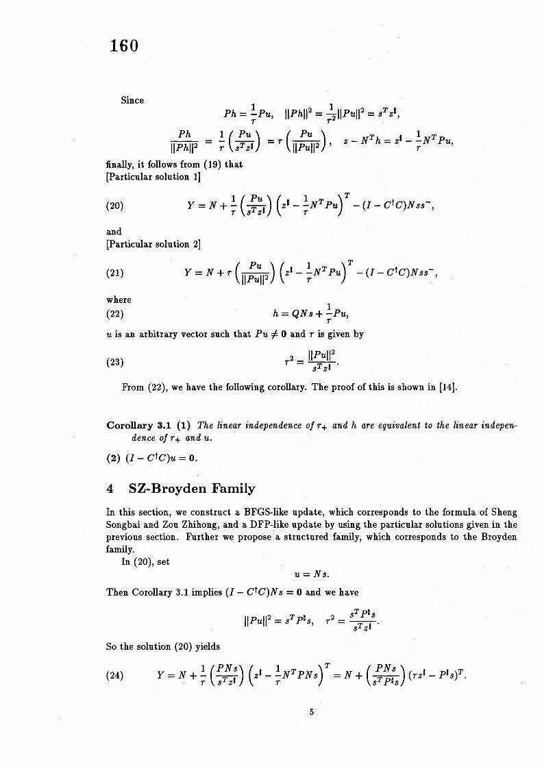
Since$Ph= \frac{1}{\tau}$Pu, $||Ph||^{2}= \frac{1}{\tau^{2}}||Pu||^{2}=s^{T}z^{1}$ ,

$\frac{Ph}{||Ph||^{2}}=\frac{1}{\tau}(\frac{Pu}{s^{T}z^{1}})=\tau(\frac{Pu}{||Pu||^{2}})$ , $z-N^{T}h=z^{1}- \frac{1}{\tau}N^{T}Pu$,

finally, it follows from (19) that[Particular solution 1]

(20) $Y=N+ \frac{1}{\tau}(\frac{Pu}{s^{T}z^{1}})(z^{1}-\frac{1}{\tau}N^{T}Pu)^{T}-(I-C^{\dagger}C)Nss^{-}$,

and[Particular solution 2]

(21) $Y=N+ \tau(\frac{Pu}{||Pu||^{2}})(z^{1}-\frac{1}{\tau}N^{T}Pu)^{\mathcal{T}}-(I-C^{\uparrow}C)Nss^{-}$,

where(22) $h=QNs+ \frac{1}{\tau}$Pu,

$u$ is an arbitrary vector such that $Pu\neq 0$ and $\tau$ is given by

(23) $\tau^{2}=\frac{||Pu||^{2}}{s^{T}z^{1}}$

From (22), we have the following corollary. The proof of this is shown in [14].

Corollary 3.1 (1) The linear independence of $r+andh$ are equivalent to the linear indepen-dence of $r+andu$ .

(2) $(I-C^{\uparrow}C)u=0$ .

4 SZ-Broyden Family

In this section, we construct a BFGS-like update, which corresponds to the formula of ShengSongbai and Zou Zhihong, and a DFP-like update by using the particular solutions given in theprevious section. Further we propose a structured family, which corresponds to the Broydenfamily.

$h(20)$ , set$u=Ns$ .

Then Corollary 3.1 implies $(I-C^{\uparrow}C)Ns=0$ and we have

11 $Pu||^{2}=s^{T}P^{\mathfrak{j}}s$ , $\tau^{2}=\frac{s^{T}P^{1}s}{s^{T}z^{1}}$

So the solution (20) yields

(24) $Y=N+ \frac{1}{\tau}(\frac{PNs}{s^{T}z^{l}})(z^{\mathfrak{j}}-\frac{1}{\tau}N^{T}PNs)^{T}=N+(\frac{PNs}{s^{T}P^{1_{S}}})(\tau z^{\mathfrak{j}}-P^{1}s)^{T}$ .

5

161

Setting $Y=L++J+andN=PL+J+$ , we have

$L_{+}^{BFGS}=PL+( \frac{PNs}{s^{T}P^{1}s})(\tau z^{1}-P^{t}s)^{T}$ ,

which is the updating formula of Sheng Songbai and Zou Zhihong.Here, setting $B+=Y^{T}Y$ gives

$B+=(P^{[}- \frac{P^{1}ss^{T}P^{1}}{s^{T}P^{1_{S}}}+\frac{z^{1}(z^{1})^{T}}{s^{T}z^{1}})+Q^{[}$ .

The above corresponds to a BFGS update from $P^{1}$ to $B+except$ for $Q^{\downarrow}$ , so we call this aSZ-BFGS update. We summarize as follows;(SZ-BFGS update)

(25) $L_{+}^{BFGS}$ $=$ $PL+( \frac{PNs}{s^{T}P^{1_{S}}})(\tau z^{\}}-P^{[}s)^{T}$ ,

(26) $\tau^{2}$

$=$$\frac{s^{T}P^{1_{S}}}{s^{T}z^{1}}$

(27) $B_{+}^{BFGS}$ $=$ $(P^{[}- \frac{P^{1}ss^{T}P^{1}}{s^{T}P^{t_{S}}}+\frac{z^{1}(z^{1})^{T}}{s^{T}z^{1}})+Q^{\#}$

$=$$B^{1}- \frac{P^{1}ss^{T}P^{1}}{s^{T}P^{1_{S}}}+\frac{z^{1}(z^{1})^{T}}{s^{T}z^{1}}$ .

In the below, we assume that the matrix $P^{1}$ is nonsingular. In (21), setting

$u=N(P^{1})^{-1}z^{1}$ and $s^{-}=( \frac{z^{1}}{s^{T}z^{1}}I^{T}$ ,

we have$||Pu||^{2}=(z^{[})^{T}(P^{\mathfrak{j}})^{-1}z^{1}$ , $N^{T}Pu=z^{t}$ , $\tau^{2}=\frac{(z^{1})^{T}(P^{t})^{-1_{Z}\#}}{s^{T}z^{1}}$ .

The result (3) of Theorem 2.2 means

$0=(I-C^{\dagger}C)(Ns-PNs+ \frac{1}{\tau}PN(P^{1})^{-1}z^{\mathfrak{j}})$

and$(I-C^{\uparrow}C)Ns=-(I-C^{\uparrow}C)PNb$, $b= \frac{1}{\tau}(P^{\int})^{-1}z^{\#}-s$ .

Noting that $C^{\uparrow}CPNb=(b^{T}z^{[})(Pu/||Pu||^{2})$ , we have

$Y$ $=$ $N+( \tau-1)(\frac{Pu}{||Pu||^{2}})(z^{[})^{T}+PNb(\frac{z^{1}}{s^{T}z^{1}})^{T}-(\tau-1)(\frac{Pu}{||Pu||^{2}})(z^{\#})^{T}$

(28) $=$ $N+PNb( \frac{z^{1}}{s^{T}z^{1}}I^{T}$

So setting $Y=L++J+andN=PL+J+$ , we have a SZ-DFP update:

6

162

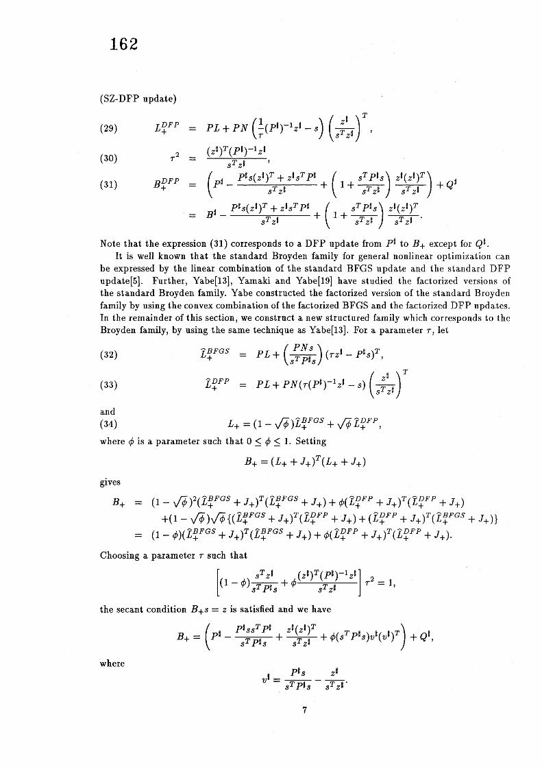
(SZ-DFP update)

(29) $L_{+}^{DFP}$ $=$ $PL+PN( \frac{1}{\tau}(P^{\{})^{-1}z^{\mathfrak{j}}-s)(\frac{z^{1}}{s^{T}z\#}I^{T}$ ,

(30) $\tau^{2}$

$=$$\frac{(z^{1})^{T}(P^{t})^{-1}z^{1}}{s^{T}z^{1}}$

(31) $B_{+}^{DFP}$ $=$ $(P^{\#}- \frac{P^{t}s(z^{1})^{T}+z^{\mathfrak{p}}s^{T}P^{t}}{s^{T}z^{1}}+(1+\frac{s^{T}P^{t_{S}}}{s^{T}z\#})\frac{z\#(z^{t})^{T}}{s^{T}z\#})+Q\#$

$=$ $B^{\downarrow}- \frac{P^{\{}s(z^{t})^{T}+z^{1}s^{T}P^{1}}{s^{T}z\#}+(1+\frac{s^{T}P^{t_{S}}}{s^{T}z^{1}})\frac{z\#(z^{\oint})^{T}}{s^{T}z\#}$

Note that the expression (31) corresponds to a DFP update from $P^{\mathfrak{p}}$ to $B+except$ for $Q^{\#}$ .It is well known that the standard Broyden family for general nonlinear optimization can

be expressed by the linear combination of the standard BFGS update and the standard DFPupdate[5]. Further, Yabe[13], Yamaki and Yabe[19] have studied the factorized versions ofthe standard Broyden family. Yabe constructed the factorized version of the standard Broydenfamily by using the convex combination of the factorized BFGS and the factorized DFP updates.In the remainder of this section, we construct a new structured family which corresponds to theBroyden family, by using the same technique as Yabe[13]. For a parameter $\tau$ , let

(32) $\hat{L}_{+}^{BFGS}$ $=$ $PL+( \frac{PNs}{s^{T}P^{1_{S}}})(\tau z^{[}-P^{t}s)^{T}$ ,

(33) $\hat{L}_{+}^{DFP}$ $=$ $PL+PN( \tau(P\#)^{-1}z^{\#}-s)(\frac{z\#}{s^{T}z\#}I^{T}$

and(34) $L_{+}=(1-\sqrt{\phi})\hat{L}_{+}^{BFGS}+\sqrt{\phi}\hat{L}_{+}^{DFP}$ ,

where $\phi$ is a parameter such that $0\leq\phi\leq 1$ . Setting

$B_{+}=(L_{+}+J_{+})^{T}(L_{+}+J_{+})$

gives

$B+$ $=$ $(1-\sqrt{\phi})^{2}(\hat{L}_{+}^{BFGS}+J_{+})^{T}(\hat{L}_{+}^{BFGS}+J_{+})+\phi(\hat{L}_{+}^{DFP}+J_{+})^{T}(\hat{L}_{+}^{DFP}+J_{+})$

$+(1-\sqrt{\phi})\sqrt{\phi}\{(\hat{L}_{+}^{BFGS}+J_{+})^{T}(\hat{L}_{+}^{DFP}+J_{+})+(\hat{L}_{+}^{DFP}+J_{+})^{T}(\hat{L}_{+}^{BFGS}+J_{+})\}$

$=$ $(1-\phi)(\hat{L}_{+}^{BFGS}+J_{+})^{T}(\hat{L}_{+}^{BFGS}+J_{+})+\phi(\hat{L}_{+}^{DFP}+J_{+})^{T}(\hat{L}_{+}^{DFP}+J_{+})$ .

Choosing a parameter $\tau$ such that

$[(1- \phi)\frac{s^{T}z^{1}}{s^{T}P^{1_{S}}}+\phi\frac{(z^{1})^{T}(P^{1})^{-1}z^{t}}{s^{T}z^{1}}]\tau^{2}=1$,

the secant condition $B_{+}s=z$ is satisfied and we have

$B+=(P^{t}- \frac{P^{t}ss^{T}P^{1}}{s^{T}P^{1_{S}}}+\frac{z^{1}(z^{1})^{T}}{s^{T}z^{1}}+\phi(s^{T}P^{[}s)v^{t}(v^{[})^{T})+Q^{\#}$ ,

where$v^{I}= \frac{P^{1_{S}}}{s^{T}P^{1_{S}}}-\frac{z^{[}}{s^{T}z^{1}}$ .

7

163

Now we obtain a new family, called a SZ-Broyden family, as follows:(SZ-Broyden family)

(35) $L+=PL+(1- \sqrt{\phi})(\frac{PNs}{s^{\mathcal{T}}Pt_{S}})(\tau z^{\#}-P^{1}s)^{T}+\sqrt{\phi}PN(\tau(P^{\#})^{-1}z^{\#}-s)(\frac{z\#}{s^{T}z\#})^{T}$

where

(36) $0\leq\emptyset\leq 1$ , $[(1- \phi)\frac{s^{T}z^{t}}{s^{T}P^{1_{S}}}+\phi\frac{(z^{1})^{T}(P\#)^{-1_{Z}\#}}{s^{T}z\#}]\tau^{2}=1$ ,

(37) $B+$ $=$ $(P^{t}- \frac{P^{1}ss^{T}P^{t}}{s^{T}P^{t_{S}}}+\frac{z^{1}(z^{1})^{T}}{s^{T}z\#}+\phi(s\tau P\# s)v^{t}(v^{t})^{T})+Q\#$

$=$ $(1-\phi)B_{+}^{BFGS}+\phi B_{+}^{DFP}$ ,

(38) $v^{t}$$=$

$\frac{P^{1}s}{s^{T}P^{t_{S}}}-\frac{z^{t}}{s^{T}z\#}$ ,

and the matrices $B_{+}^{BFGS}$ and $B_{+}^{DFP}$ are given in (27) and (31), respectively.Note that the expression (37) corresponds to a Broyden family from $P\#$ to $B+except$ for

$Q^{t}$ . Setting $\phi=0$ and $\phi=1$ yields the SZ-BFGS update (25) and the SZ-DFP update (29),respectively.

5 Other types of Structured Broyden Family

In the previous section, we propose the SZ-Broyden family based on the idea of Sheng Songbaiand Zou Zhihong. The subjects of this section are to introduce the $structu\iota ed$ Broyden familygiven by Yabe and Yamaki[18] and to consider the relationship between our family and thestructuted secant update from the convex class proposed by Martinez[10].

Consider the case where we do not impose the condition $L_{+}^{T}r+=0$ on the matrix $L+for$ theSZ-BFGS update. Since $P=I$, we have

$N=L+J+$ , $Q=0$ , $Q^{\#}=0$ , $z^{\#}=z$ , $P^{\#}=B\#$ .

Thus the update (25) is reduced to the BFGS-like update given by Yabe and Takahashi[15]:

(39) $L+$ $=$ $L+( \frac{(L+J_{+})s}{s^{T}B^{1}s})(\tau z-B^{1}s)^{T}$,

(40) $\tau^{2}$

$=$$\frac{s^{T}B^{[}s}{s^{T_{Z}}}$ $B\#=(L+J_{+})^{T}(L+J_{+})$ ,

(41) $B+$ $=$ $B^{1}- \frac{B^{1}ss^{T}B^{t}}{s^{T}B^{1_{S}}}+\frac{zz^{T}}{s^{T}z}$ .

Here we can regard the matrices $(L+J_{+})^{T}(L+J_{+})$ and $(L_{+}+J_{+})^{T}(L++J_{+})$ as the matrices$J_{+}^{T}J_{+}+A$ and $J_{+}^{T}J_{+}+A_{+}$ , respectively. So, setting

(42) $B^{\mathfrak{j}}=J_{+}^{T}J++A$ , and $B+=J_{+}^{T}J++A+$

in (41), we have an updating formula for $A$

(43) $A+=A- \frac{ww^{\mathcal{T}}}{s^{T}w}+\frac{zz^{\prime r}}{s^{T_{Z}}}$, $w=(J_{+}^{T}J_{+}+A)s$ ,

8

164

whish is the structured BFGS update given by Al-Baali and Fletcher[l]. Thus the expression(39) corresponds to the factorized form of the structured BFGS update of Al-Baali and Fletcher.

Consider the case where we do not impose the condition $L_{+}^{T}r+=0$ on the matrix $L_{+}$ for theSZ-DFP update. Then the update (29) is reduced to the DFP-like update given by Yabe andTakahashi[15]:

(44)$|$

$L+$ $=$ $L+(L+J_{+})( \frac{1}{\tau}(B^{1})^{-1}z-s)(\frac{z}{s^{T_{Z}}})^{T}$ ,

(45) $\tau^{2}$

$=$ $\frac{z^{T}(B^{1})^{-1}z}{s^{T}z}$

(46) $B+$ $=$ $B^{\mathfrak{j}}- \frac{B^{1}sz^{T}+zs^{T}B^{1}}{s^{T}z}+(1+\frac{s^{T}B^{1}s}{s^{T}z})\frac{zz^{T}}{s^{T}z}$

Substituting (42) for (46), we have an updating formula for $A$

(47) $A+$ $=$ $A+ \frac{(q-As)z^{T}+z(q-As)^{T}}{s^{T_{Z}}}-\frac{s^{T}(q-As)}{(s^{T}z)^{2}}zz^{T}$ ,

$q$ $=$ $(J_{+}-J)^{T}r+$ ,

which is the revised update of Dennis, Gay and Welsch[6]. Thus the expression (44) correspondsto the factorized form of the DGW update.

Further, consider the case where we do not impose the condition $LTr+=0$ on the matrix$L_{+}$ for the SZ-Broyden family. Then the family (35) is reduced to the structured Broyden familygiven by Yabe and Yamaki[18]:

(48) $L+$ $=$ $L+(1- \sqrt{\phi})(\frac{(L+J_{+})s}{s^{T}B^{1_{S}}})(\tau z-B^{1}s)^{T}$

$+ \sqrt{\phi}(L+J_{+})(\tau(B^{\mathfrak{j}})^{-1}z-s)(\frac{z}{s^{T_{Z}}})^{T}$ ,

(49) $B+$ $=$ $B^{1}- \frac{B^{1}ss^{T}B^{[}}{s^{T}B^{1}s}+\frac{zz^{T}}{s^{T_{Z}}}+\phi(s^{T}B^{1}s)vv^{T}$ ,

where(50)

$\tau^{2}=\frac{1}{(1-\phi)\frac{s^{T_{Z}}}{s^{T}B^{1_{S}}}+\phi\frac{z^{T}(B^{1})^{-1}z}{s^{T_{Z}}}}$

, $v= \frac{B^{I_{S}}}{s^{T}Bt_{S}}-\frac{z}{s^{T_{Z}}}$.

As the same way of the above, substituting (42) for (49), we have an updating formula for $A$

(51) $A+=A- \frac{ww^{T}}{s^{q}’ w}+\frac{zz^{T}}{s^{T_{Z}}}+\phi(s^{T}w)vv^{T}$ ,

$v= \frac{w}{s^{T}w}-\frac{z}{s^{T_{Z}}}$ , $w=(J_{+}^{T}J_{+}+A)s$ , $0\leq\emptyset\leq 1$ ,

which is the structured secant update from the convex class proposed by Martinez[10]. Thusthe expression (48) corresponds to the factorized form of the structured secant update from theconvex class.

FinaUy, we apply sizing techniques given by Bartholomew-Biggs[2], Dennis, Gay and Welsch[6]to the above and obtain the following sized family:

(52) $A+= \beta A-\frac{ww^{T}}{s^{T}w}+\frac{zz^{T}}{s^{T_{Z}}}+\phi(s^{T}w)vv^{T}$ ,

9

165

$v= \frac{w}{s^{T}w}-\frac{z}{s^{T_{Z}}}$ , $w=(J_{+}^{T}J_{+}+\beta A)s$ , $0\leq\phi\leq 1$ .

Here $\beta$ is defined by the Bartholomew-Biggs’ parameter

(53) $\beta=\frac{r_{+}^{T}r}{r^{T}r}$

or by the DGW parameter

(54) $\beta=\min(|\frac{s^{T}q}{s^{T}As}|,$ $1)$ .

References[1] M.Al-Baali and R.Fletcher: Variational methods for non-linear least squares, Journal of the Oper-

ational Research Society, Vol.36 (1985), pp.405-421.[2] M.C.Bartholomew-Biggs: The estimation of the Hessian matrix in nonlinear least squares problems

with non-zero residuals, Mathematical Programming, Vol.12 (1977), pp.67-80.[3] A.Ben-Israel and T.N.E.Greville : Generalized Inverses – Theory and Applications, Robert E.

Krieger Publishing Company, Huntington, 1980.[4] J.E.Dennis,Jr. : A brief survey of convergence results for quasi-Newton methods, SIAM-AMS Pro-

ceedings, Vol.9 (1976), pp.185-199.[5] J.E.Dennis,Jr. and R.B.Schnabel: Numerical Methods for Unconstrained optimization and Nonlin-

ear Equations, Prentice-Hall, New Jersey, 1983.[6] J.E.Dennis,Jr., D.M.Gay and R.E.Welsch : An adaptive nonlinear least squares algorithm, A CM

Transactions on Mathematical Software, Vol.7, No.3, (1981), pp.348-368.[7] J.E.Dennis,Jr., S.Songbai and P.A.Vu : A memoryless augmented Gauss-Newton method for non-

linear least-squares problems, Technical Report 85-1, Department of Mathematical Sciences, RiceUniversity (1985).

[8] J.E.Dennis,Jr., H.J.Martinez and R.A.Tapia: Convergence theory for the structured BFGS secantmethod with an application to nonlinear least squares, Journal of optimization Theory and Appli-cations, Vol.61 (1989), pp.161-178.

[9] R.Fletcher and C.Xu : Hybrid methods for nonlinear least squares, IMA J. Numerical Analysis,Vol.7 (1987), pp.371-389.

[10] H.J.Martinez R. : Local and superlinear convergence of structured secant methods from the convexclass, PhD Thesis, Rice University, 1988.

[11] Sheng Songbai and Zou Zhihong: A new secant method for nonlinear least squares problems, Tech-nical Report NANOG-1988-03, Nanjing University (1988).

[12] C.X.Xu : Hybrid method for nonlinear least-square probleIns without calculating derivatives, Jour-nal of optimization Theory and Applications, Vol.65, No.3 (1990), pp.555-574.

[13] H.Yabe: A family of variable-metric methods with factorized expressions, TRU Mathematics, Vol.17,No. 1 (1981), pp.141-152.

[14] H.Yabe : Generalization of the Sheng Songbai and Zou Zhihong method for solving nonlinear leastsquares problems, Studies in Liberal Arts and Sciences, Vol.23, Science University of Tokyo, inJapanese (1990) to appear.

[15] H.Yabe and T.Takahashi : Structured quasi-Newton methods for nonlinear least squares problems,TRU Mathematics, Vol.24, No.2, (1988), pp.195-209.

[16] H.Yabe and T.Takahashi: Numerical comparison among structured quasi-Newton methods for non-linear least squares problems, Research Report (Kokyuroku), Vol.717, Research Institute for Mathe-matical Sciences, Kyoto University (1990), pp. 144-158.

[17] H.Yabe and T.Takahashi : Factorized quasi-Newton methods for nonlinear least squares problems,Mathematical Programming, to appear.

[18] H.Yabe and N.Yamaki: Convergence of structured quasi-Newton methods with structured Broydenfamily, Research Report, The Institute of Statistical Mathematics, in Japanese (1991) to appear.

[19] N.Yamaki and H.Yabe : On factorized variable-metric methods, TRU Mathematics, Vol.17, No.2(1981), pp.285-294.

10