5Topological insulators Part I: Phenomena

5.1. Quantum Hall effect

5.1.1. Hall effect

◼ Consider electrons moving in a 2D plane (the system is known as a 2D electron gas or 2DEG). If we apply an in-plane electric field E, we

will get some electric current j. Typically, E // J. Let’s assume they are in the x direction Ex and jx. The resistivity is ρxx = Ex / jx

◼ Apply a B field perpendicular to the 2D plane. Lorentz force leads to charge accumulation for the top and bottom edge. This gives a E field

perpendicular to the current (Ey). Hall resistivity: ρxy = Ey / jx

◼ The rotational symmetry tells us that ρxx = ρyy and ρxy = ρyx

◼ Classical mechanics: ρxy ∝ B

e Ey = e v B (5.1)

jx = e v n (5.2)

ρxy = Ey / jx =v B

e v n=B

e n(5.3)

Fig. 1. the Hall effect

Phys540.nb 71

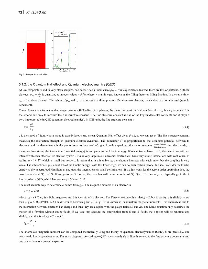
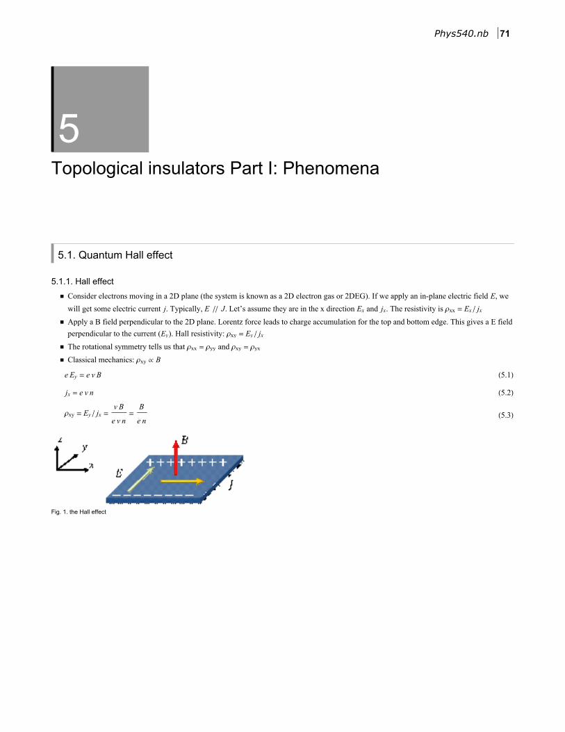
Fig. 2. the quantum Hall effect

5.1.2. the Quantum Hall effect and Quantum electrodynamics (QED)

At low temperature and in very clean samples, one doesn’t see a linear curve ρxy ∝ B in experiments. Instead, there are lots of plateaus. At these

plateaus, σxy =1ρxy

is quantized to integer values ν e2 h, where ν is an integer, known as the filling factor or filling fraction. In the same time,

ρxx = 0 at these plateaus. The values of ρxx and ρxy are universal at these plateaus. Between two plateaus, their values are not universal (sample

dependent).

These plateaus are known as the integer quantum Hall effect. At a plateau, the quantization of the Hall conductivity σxy is very accurate. It is

the second best way to measure the fine structure constant. The fine structure constant is one of the key fundamental constants and it plays a

very important role in QED (quantum electrodynamics). In CGS unit, the fine structure constant is

α =e2

ℏ c(5.4)

c is the speed of light, whose value is exactly known (no error). Quantum Hall effect gives e2 h, so we can get α. The fine structure constant

measures the interaction strength in quantum electron dynamics. The numerator e2 is proportional to the Coulomb potential between to

electrons and the denominator is the proportional to the speed of light. Roughly speaking, this ratio computes potential enrgykinetic energy

, in other words, it

measures how strong the interaction (potential energy) is compares to the kinetic energy. If our universe have α = 0, then electrons will not

interact with each other (a free electron system). If α is very large in our universe, electron will have very strong interactions with each other. In

reality, α ~ 1 /137, which is small but nonzero. It means that in this universe, the electron interacts with each other, but the coupling is very

weak. The interaction is just about 1% of the kinetic energy. With this knowledge, we can do perturbation theory. We shall consider the kinetic

energy as the unperturbed Hamiltonian and treat the interactions as small perturbations. If we just consider the zeroth order approximation, the

error bar is about O(α)~1 %. If we go to the 3rd order, the error bar will be in the order of Oα4~10-8. Currently, we typically go to the 4

fourth order in QED, which has accuracy of about 10-10.

The most accurate way to determine α comes from g-2. The magnetic moment of an electron is

μ = g μB S /ℏ (5.5)

where μB = e ℏ /2me is a Bohr magneton and S is the spin of an electron. The Dirac equation tells us that g = 2, but in reality, g is slightly larger

than 2, g = 2.0023193043622 The difference between g and 2 (i.e. g - 2) is known as “anomalous magnetic moment”. This anomaly is due to

the interaction between electrons has charge and thus they are coupled with the gauge fields (E and B). The Dirac equation only describes the

motion of a fermion without gauge fields. If we take into account the contribution from E and B fields, the g-factor will be renormalized

slightly, and this is why g - 2 is not 0.

δg =g - 2

2(5.6)

The anomalous magnetic moment can be computed theoretically using the theory of quantum electrodynamics (QED). More precisely, one

needs to do loop expansions using Feynman diagrams. According to QED, the anomaly δg is directly related to the fine structure constant α and

one can write a as a power expansion

72 Phys540.nb

δg =α

2 π+ #2 α2 + #3 α3 + #4 α4 + ... (5.7)

Currently, we know the first 4 coefficients. Because α is very small ~ 1137

, the contributions from the higher order terms are very small (in the

order of 10-10). If we ignore the higher order terms, we can get α from g - 2.

Remarks:

◼ For measuring α, g-2 gives a more accurate result than IQH. the error bar from g-2 is 0.37×10-9. Using IQH, it is 24×10-9

◼ On the other hand, to get α from g-2, one needs to assume that the theory of QED is correct. But IQH offers a measurement of α

independent of QED. The fact that these two measurements agree with each other offers a direct verification of the theory of QED.

◼ A condensed matter experiment which is almost as accurate as QED, this is very unusual and special.

The difference between theories and experiments in condensed matter physics is typically in the range of a few percent to a few hundred

percent (sometimes, it could be even larger). The error bar here is much larger than atomic/particle physics, especially QED. This is because (2

reasons)

◼ Solids are typically very dirty. There are lots of impurities. These impurities make our data noisy.

◼ Most condensed matter systems are strongly correlated (in comparison to QED), and thus it is much harder to handle theoretically.

◼ QED: the strength of interactions is set by the fine structure constant, which is very small, so we can do perturbation theory.

α =e2

ℏ c~1137 (5.8)

◼ CMP: the strength of interactions takes a similar form, but the speed of light now turns into the Fermi velocity. Fermi velocity vF is

typically 1/100-1/1000 of c, so the “fine structure constant” of solids is about 100-1000 times larger.

αCMP =e2

ℏ vF

~ 1 - 10 (5.9)

◼ For such a large αCMP, perturbation theory cannot be trusted.

Q: Why is σxy so accurate in the IQHE?

A: This is a very special quantum state where interactions and impurities plays no role. (Please keep these questions and we will come back to

them later, after we learn more about TIs). This state is actually a topological state of matter, where the Hall conductivity is determined by the

topology of the quantum wave-function and the topology doesn’t care about interactions and impurities.

5.1.3. Why ρxx = 0?

Now let’s look at ρxx, which is 0 in a quantum Hall state.

◼ Q: Zero resistivity ρxx. Is this state a superconductor or a perfect metal?

◼ A: No. It is not a perfect conductor, neither a superconductor. It is not even a conductor. It is actually an insulator. This material has zero

conductivity.

Two equations that we are very familiar with:

j = σ E (5.10)

E = ρ j (5.11)

and

ρ = 1 /σ (5.12)

This naive formula requires a very important assumption: j and E are in the same direction. If we apply E in the x direction, the current must

also in the x direction and there cannot be any jy, and vice versa. This assumption is true sometimes, but not always.

A more generic formula:

jxjyjz

=

σxx σxy σxz

σyx σyy σyz

σzx σzy σzz

ExEyEz

(5.13)

Phys540.nb 73

If all off-diagonal terms are zero (σxy = σyz = σzx = 0) and all the diagonal terms are the same we got:

j = σ E (5.14)

So ρ =1

σ(5.15)

THE KEY: conductivity is a tensor (a d×d matrix), instead of a scalar. For an isotropic system, the metrix reduces into an number

σxx σxy σxz

σyx σyy σyz

σzx σzy σzz

= σ1 0 00 1 00 0 1

(5.16)

But this is NOT true for generically.

For 2D

jxjy =

σxx σxy

σyx σyy ExEy

(5.17)

◼ Q: How about resistivity?

◼ A: Of course, it is also a matrix

ExEy

= ρxx ρxy

ρyx ρyy jxjy (5.18)

◼ Q: What’s the relation between conductivity and resistivity?

◼ A: They are matrix inverse of each other.

σxx σxy

σyx σyy =

ρxx ρxy

ρyx ρyy-1

=1

ρxx ρyy - ρxy ρyx

ρyy -ρxy

-ρyx ρxx (5.19)

For a quantum Hall system, at each plateaus: ρxx = ρyy = 0, so the resistivity is an off-diagonal matrix

ρxx ρxy

ρyx ρyy =

0 ρxy

ρyx 0 (5.20)

The conduits tensor is its matrix inverse,

σxx σxy

σyx σyy =

1

-ρxy ρyx

0 -ρxy

-ρyx 0 =

0 1 /ρyx

1 /ρxy 0 (5.21)

Here, we find that the diagonal terms σxx and σyy are zero, which means that we don’t have any conductivity, so the system is actually an

insulator.

Between two IQH plateaus (ρxx is nonzero), σxx and σyy is nonzero. So the system is a metal.

σxx σxy

σyx σyy =

1

ρxx ρyy - ρxy ρyx

ρyy -ρxy

-ρyx ρxx (5.22)

5.1.4. Summary

From this point of the view, we can summarize the IQHE as the following,

◼ By varying the strength of the B field, the systems turns from one insulator to a metal, then another insulator, a metal …

◼ Each insulating state corresponds to a plateau of ρxy and the step between two neighboring plateaus is a metallic state.

◼ The transport coeffcients for the metallic states are non-universal, which varies from sample to sample.

◼ The insulating states are very universal (independent of samples). They have zero ρxx and zero σxx, and the Hall conductivity σxy is

quantized.

The following sections answers two questions

◼ Why are these IQH states insulators?

◼ Why these insulators has quantized Hall conductivity?

74 Phys540.nb

5.2. Why the IQH states are insulators? This is due to the formation of Landau levels

5.2.1. The Schrodinger equation for a particle with charge e (the minimal coupling)

Consider a charge neutral particle moving in a 2D plane (the charge q = 0). The Schrodinger equation is

ⅈ ∂ tψ(x, y) = 1

2m(-ⅈ ℏ ∂x)2 +

1

2m(-ⅈ ℏ ∂y)2 ψ(x, y) (5.23)

H =1

2m(-ⅈ ℏ ∂x)2 +

1

2m(-ⅈ ℏ ∂y)2 (5.24)

If this particle has charge e, we need to add the E and B fields into the equation, because charged particles couple to the E and B fields.

To introduce the E&B fields, we use the minimal coupling, which tells us that we need to change the momentum operator p→ into p→ + e A→c,

where A→

is the vector potential, and change ⅈ ∂ t into ⅈ ∂ t-e Φ /c, where Φ is the Electric potential.

(ⅈ ∂ t-e Φ /c) ψ(x, y) = 1

2m-ⅈ ℏ ∂x-

e

cAx

2+

1

2m-ⅈ ℏ ∂y-

e

cAy

2 ψ(x, y) (5.25)

ⅈ ∂ t ψ(x, y) = 1

2m-ⅈ ℏ ∂x-

e

cAx

2+

1

2m-ⅈ ℏ ∂y-

e

cAy

2 + e Φ /c ψ(x, y) (5.26)

H =1

2m-ⅈ ℏ ∂x-

e

cAx

2+

1

2m-ⅈ ℏ ∂y-

e

cAy

2+ e Φ /c (5.27)

For us, E = 0, so we can set the electric potential Φ = 0. The vector potential satisfies

∇ ×A = ∂x Ay - ∂y Ax = B (5.28)

As we learned in E and M, the vector potential A is NOT a physical observable. For a fixed B field, A is not uniquely determined. If A is the

vector potential for B (∇ ×A = B), A ' = A + ∇ χ is also the vector potential for the same B field (∇ ×A ' = B). We can choose A arbitrarily, as

long as the curl of A is the same. For us, B is along the z-axis and it is a constant (a uniform magnetic field). Typically, one use one of the

following two options:

Ax = 0 and Ay = B x (the Landau gauge) (5.29)

Ax = -B y

2and Ay =

B x

2(the symmetric gauge) (5.30)

5.2.2. Energy spectrum and Landau levels

If we choose the Landau gauge,

H = ℏ2

2m(-ⅈ ∂x)2 +

1

2m-ⅈ ℏ ∂y-

e

cB x

2 (5.31)

◼ Q: Eigenstates of H? H ψ = ϵ ψ

In the Landau gauge, [py, H] = 0. Therefore, we can find common eigenstates for py and H . This tells us that the eigen states of H can be

written in the following form.

ψ(x, y) = f (x) exp(-ⅈ ky y) (5.32)

This wave-function is a comment eigenstates of H and py. For the momentum operator py, its eigenvalue is ℏ ky. Put this wave-function into the

static Schrodinger equation, we find

-ℏ2

2mf '' (x) +

1

2mℏ ky -

e

cB x

2f (x) = ϵ f (x) (5.33)

-ℏ2

2mf '' (x) +

e2 B2

2m c2x -

c ℏ

e Bky

2

f (x) = ϵ f (x) (5.34)

Phys540.nb 75

This equation is identical the Schrodinger equation of a harmonic oscillator:

-ℏ2

2m

ⅆ

ⅆx2ϕ (x) +

k

2(x - x0)

2 ϕ(x) = ϵ ϕ(x) (5.35)

x0 is the equilibrium position. k is the spring constant. Here, we have

x0 =c ℏ

e Bky (5.36)

k =e2 B2

m c2(5.37)

Therefore, the solution of our Schrodinger equation is exactly the same as a harmonic spring.

ψn, ky(x, y) = ϕn(x - x0) exp(-ⅈ ky y) (5.38)

ϵn,ky = n +1

2ℏ ω = n +

1

2ℏ

k

m= n +

1

2

e B ℏ

c m(5.39)

5.2.3. Landau levels as energy bands

If we plot the energy as the function of the momentum ky, we find the dispersion relation. The dispersion contains a bunch of horizontal lines,

which can be considered as energy bands.

◼ These lines (which is known as Landau levels) looks like energy bands (n is the band index and ky is the momentum)

◼ All the quantum states in one band (same n but different ky) have the same energy. This means that our energy bands here are flat.

Since we have energy bands here, we can have two possible states: if μ is located inside the gap, we have an insulator (this is a quantum Hall

plateau), but if μ happens to cross with one of the bands (Landau levels), we got a metal (this is the metallic states between plateaus).

In experiments, we typically change B with a fixed μ, instead of μ. Notice that ϵn,ky ∝ B. Therefore, when B is increased, we are increasing the

energy of all bands. Since μ is fixed, when we increase B, sometimes μ is between two bands in the gap and sometimes it crosses a Landau level

(so we see the system turns from an insulator to a metal and then to another insulator, another metal ...

5.3. Edge states and the Quantization of the Hall conductivity

5.3.1. a semi-classical picture

Consider one electron moving in a constant B field. The Lorentz force is

F→=q

cv→×B→

(5.40)

We know that in classical mechanics, when a force is perpendicular to the velocity, we will have a circular motion. The acceleration of a

circular motion is

a =v2

r=F

m=q

m cv B (5.41)

So we have

v =q

m cB r (5.42)

The period T is

T =2 π r

v=

2 π rq

m cB r

=2 πm c

q B(5.43)

The angular frequency

76 Phys540.nb

ωc = 2 π /T = q B /m c (5.44)

In quantum mechanics, we know that if we have a frequency, then we can use it to define an energy scale ℏω. Here, if we use the frequency of

this circular motion, we find an energy scale

E = e ℏ B /m c (5.45)

This is exactly the energy separation between two Landau levels. In fact, the energy of the Landau levels can be written as:

En = n +1

2ℏ ωc (5.46)

5.3.2. Chiral edge states

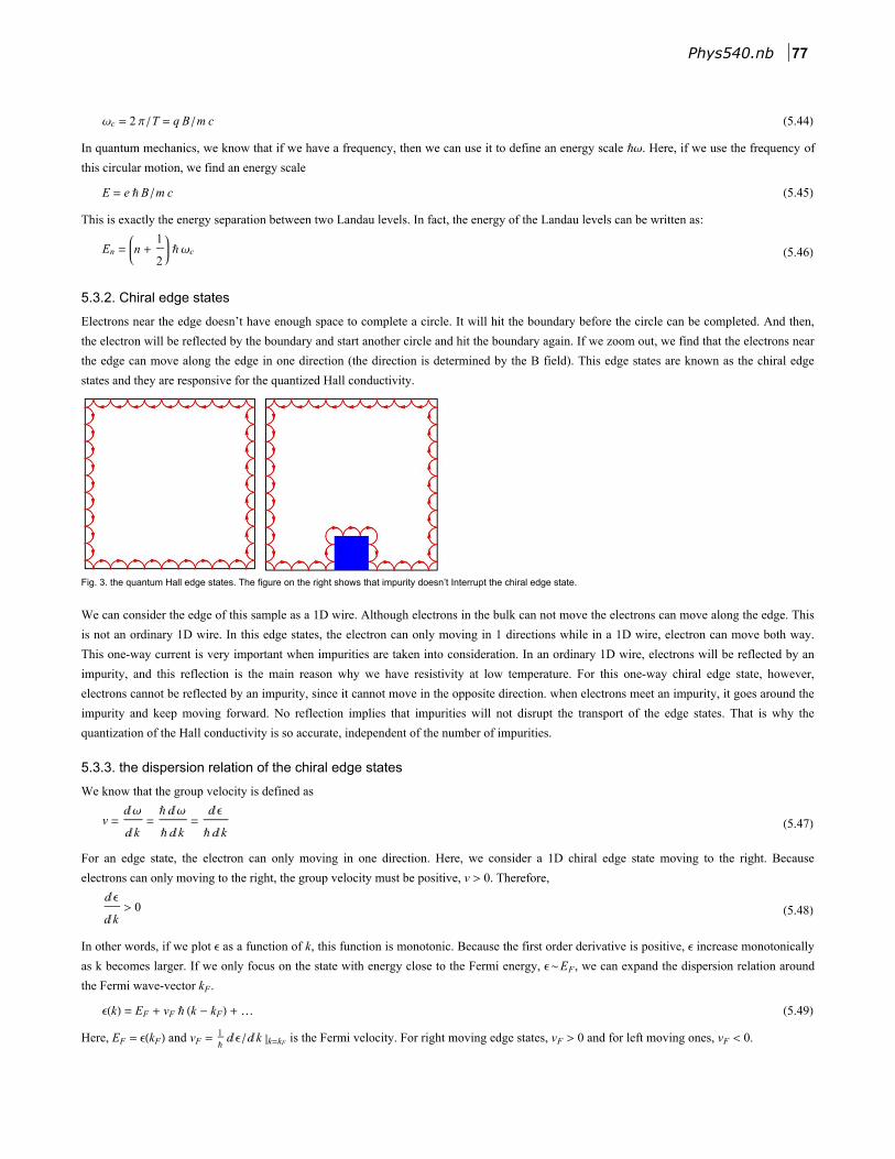
Electrons near the edge doesn’t have enough space to complete a circle. It will hit the boundary before the circle can be completed. And then,

the electron will be reflected by the boundary and start another circle and hit the boundary again. If we zoom out, we find that the electrons near

the edge can move along the edge in one direction (the direction is determined by the B field). This edge states are known as the chiral edge

states and they are responsive for the quantized Hall conductivity.

Fig. 3. the quantum Hall edge states. The figure on the right shows that impurity doesn’t Interrupt the chiral edge state.

We can consider the edge of this sample as a 1D wire. Although electrons in the bulk can not move the electrons can move along the edge. This

is not an ordinary 1D wire. In this edge states, the electron can only moving in 1 directions while in a 1D wire, electron can move both way.

This one-way current is very important when impurities are taken into consideration. In an ordinary 1D wire, electrons will be reflected by an

impurity, and this reflection is the main reason why we have resistivity at low temperature. For this one-way chiral edge state, however,

electrons cannot be reflected by an impurity, since it cannot move in the opposite direction. when electrons meet an impurity, it goes around the

impurity and keep moving forward. No reflection implies that impurities will not disrupt the transport of the edge states. That is why the

quantization of the Hall conductivity is so accurate, independent of the number of impurities.

5.3.3. the dispersion relation of the chiral edge states

We know that the group velocity is defined as

v =ⅆω

ⅆk=ℏ ⅆω

ℏ ⅆk=

ⅆϵ

ℏ ⅆk(5.47)

For an edge state, the electron can only moving in one direction. Here, we consider a 1D chiral edge state moving to the right. Because

electrons can only moving to the right, the group velocity must be positive, v > 0. Therefore,

ⅆϵ

ⅆk> 0 (5.48)

In other words, if we plot ϵ as a function of k, this function is monotonic. Because the first order derivative is positive, ϵ increase monotonically

as k becomes larger. If we only focus on the state with energy close to the Fermi energy, ϵ~EF, we can expand the dispersion relation around

the Fermi wave-vector kF.

ϵ(k) = EF + vF ℏ (k - kF) + … (5.49)

Here, EF = ϵ(kF) and vF =1ℏⅆϵ /ⅆk k=kF is the Fermi velocity. For right moving edge states, vF > 0 and for left moving ones, vF < 0.

Phys540.nb 77

Similarly, if we consider the chiral edge states moving to the left, we find that ⅆϵ /ⅆk < 0 and thus ϵ is a monotonically decreasing function of k.

We end this section by comparing the chiral edge states with an ordinary 1D wire. In an ordinary 1D wire, electrons can move to the left or

right. Therefore, the group velocity ⅆϵ /ⅆ k can take both + and - sign (depending on the value of k). The simplest case (1D free electrons) is

ϵ = ℏ2 k2 2m, where the group velocity is v = ⅆϵ /ⅆk = ℏ k /m. Here, v > 0 when k > 0 and v < 0 when k < 0. This means that if the momentum

is positive, the electron is moving to the right. When momentum is negative, the electron is moving to the left. In other words, electrons can

move in both directions. Usually, we call the k > 0 part the right moving branch and the k < 0 part the left moving branch. For an ordinary 1D

wire, we always have (at least) two branches, one moving to the left and the other moving to the right. However, for a 1D chiral edge states, we

have only one branch. In this sense, a chiral edge state is half of a 1D wire.

Finally, it is easy to notice that for a 1D wire, one shall have two Fermi wave vector kF and -kF. The Fermi velocity at these two Fermi wave

vectors take the opposite sign (one moving to the left, the other moving to the right). However, for one chiral edge state, we only have one

Fermi wave-vector.

5.3.4. Hall conductivity

We consider a Hall bar here. The circular motion of the electrons tells us that the top and bottom edge must have the opposite Fermi velocity

(one moving to the left and the other moving to the right). Here, we assume that the top edge has negative Fermi velocity (left moving) and the

bottom edge has positive Fermi velocity (right moving).

Case I: Ey = 0. Here, the top and bottom edges have the same electric potential. So we expect the number of electrons near the top edge equals

to the number of electrons near the bottom edge. This means that we have the same number of electrons moving to the right and left. Thus, the

total current along the x direction is 0.

Case II: Ey ≠ 0. Here, the top and bottom edges have different electric potentials. Let’s consider here the situation where the top edge has

electric potential +V /2, while the bottom edge has -V /2. Because we have a positive potential at the top edge, it will attract more electrons to

the top edge (electrons have charge -e and negative charge likes positive potential). For similar reasons, the bottom edge will have less number

of electrons. Therefore, the number of electrons moving to the left will be higher than the number moving to the right. So we have a net electron

flow to the left. Because electron carries negative charge, this means that we will have a current flowing to the right.

To compute this current, we need to count how many electrons got attracted to the top edge (and expel by the bottom edge). Let’s start from the

bottom edge, the energy of an electron is know its kinetic energy+the potential energy due to the -V /2 electric potential

ϵ = EF + vF ℏ(k - kF) + e V /2 (5.50)

Here, EF is the Fermi energy, vF is the Fermi velocity, kF is the Fermi wave vector before we apply the potential energy. Because electrons

carrier charge -e, the potential energy is (-e)×(-V /2) = e V /2, which is the last term.

After we applied the potential energy, the Fermi wave-vector is no longer kF, because the dispersion relation is not different. We should find the

new Fermi wave using the condition ϵ = EF

ϵ = EF + vF ℏ (k - kF) + e V /2 = EF (5.51)

ℏ vF(k - kF) = -e V /2 (5.52)

k = kF -e V

2 ℏ vF(5.53)

Before we apply the potential, electrons fills up all quantum states with k < kF. After we apply the potential, electrons fill up all quantum states

with k < kF - e V /2 vF ℏ. If we compare these two cases, it is easy to notice that if we apply the potential, the quantum states with

kF - e V /2 vF ℏ < k < kF turns from occupied to unoccupied. In other words, some electrons are expelled from the bottom edge. This is exactly

what we want to compute. The number of electrons expelled from the bottom edge by the electric potential is

Nb = kF-e V/2

kF ⅆk

2 π /Lx=Lx

2 πkF - kF -

e V

2 vF ℏ =

Lx

2 πe V /2 =

Lx

2 π

e V

2 vF ℏ(5.54)

Notice that here we don’t have the factor of 2. For systems without magnetic field, we usually have a factor 2 for electrons when we count the

number of quantum states, because electrons have spin 1/2. Here, we don’t have this factor, because the magnetic field is very strong, such that

78 Phys540.nb

the spins of electrons are essentially polarized (all aligned in the direction of B). So we don’t have the factor 2 anymore.

Because current j = -e n vF, where n is the density of electrons, the change of current due to the change of electron number is δ j = -e δ n vF

Here, the number of right moving electrons is reduced by Nb, so that the change of density δn = -Nb /Lx /Ly. So we have

δjx(b) = (-e) -Nb

Lx LyvF = e

1

2 π

e V

2 vF Ly ℏvF =

e2

h

V

2 Ly=e2

h

Ey

2(5.55)

Here, Ey = V /Ly is the strength of the electric field in the y direction (perpendicular to the current).

Similarly, we can do the same calculation for the top edge and we will get that

δjx(t) =e2

h

Ey

2(5.56)

If we combine the contributions from both edges together, we find

jx = δjx(t) + δjx(b) =e2

hEy (5.57)

Thus, we have

σxy =jx

Ey=e2

h(5.58)

The bottom line, for one chiral edge state, we get σxy = e2 h. If we have n chiral edge states, σxy = n e2 h. Notice that n here is the number of

edge states, which must be an integer. This is the reason why the Hall conductivity must take integer values.

It can be shown that each filled Landau level gives us one chiral edge states. Therefore, the number of chiral edge states (or say the Hall

conductivity) is just the number of filled Landau levels.

5.4. Topology and insulators

5.4.1. Gauss–Bonnet theorem and topology

The idea of topology originates from geometry which describes manifolds in a 3-dimensional space. Later, it is generalized other dimensions

and generic abstract space (including the Hilbert space in quantum physics). In geometry, if an manifold M1 can be adiabatically deformed into

M2, we say that they have the same topology. Otherwise, we say that they are topologically different. Examples: the surface of a sphere and the

surface of a cube are topologically equivalent, while the surface of a sphere and the surface of donut (a torus) are topologically different.

To distinguish different manifolds, mathematicians developed an object, which is called an “index” (a topological index). It is an integer

number. For objects with the same topology, the index takes the same value. Otherwise, the values are different. For 2D closed manifold, the

index is the Euler characteristic:

χM =1

2 π

M

K ⅆS (5.59)

To define the curvature for a curve, we use a circle to fit the curve around one point on the curve. The inverse radius κ=1/R gives us the

curvature.For a manifold, one can draw lots of curves at one point and one can get the curvature for each of these curves. Among all these

curvatures, the largest and smallest are known as the principle curvatures κ1 and κ2. The Gaussian curvature is the product of they two. For a

sphere, κ1 = κ2 = 1 /R, so K =1R2 . For a saddle point, the surface curves up along one direction and curves down along another direction, so that

we have κ1 > 0 and κ2 < 0. As a result, K = κ1 κ2 < 0.

For 2D closed manifold, the total Gaussian curvature (∯MK ⅆS) is always 2π times an integer. Therefore, the value of χM is quantized to

integer. For manifolds with the same topology, its value is the same. (For orientable closed manifolds, χM can only be even integers. Here

orientable means that we can distinguish two sides of this surface. There are some 2D surfaces, which one cannot distinguish the two surfaces,

e.g. a Möbius strip, and there χM can be odd).

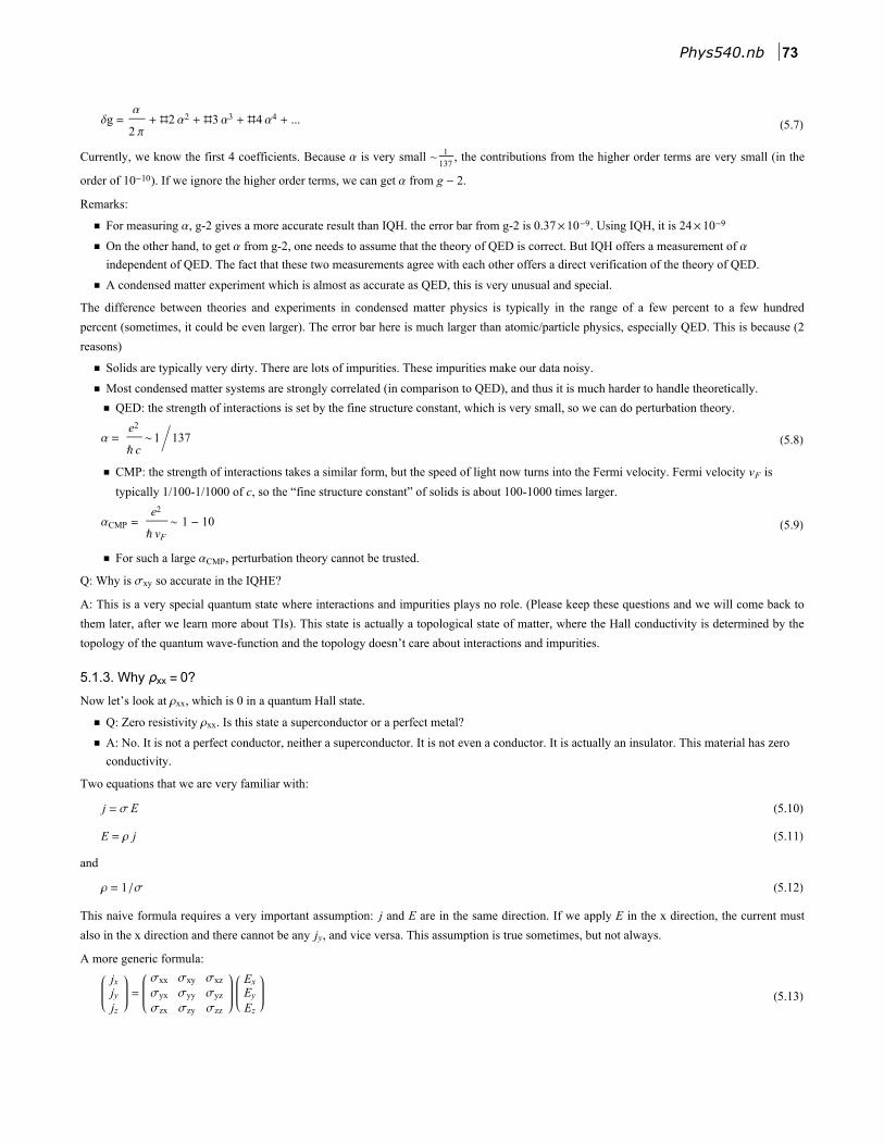
Sphere : χM = 2

Phys540.nb 79

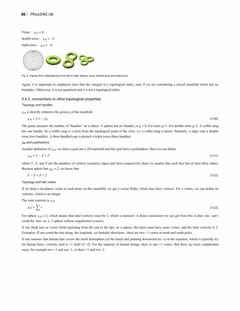
Torus : χM = 0

double torus : χM = -2

triple torus : χM = -4

Fig. 4. Figures from wikipedia.org From left to right: sphere, torus, double torus and triple torus.

Again, it is important to emphasize here that this integral is a topological index, only if we are considering a closed manifold which has no

boundary. Otherwise, it is not quantized and it is not a topological index.

5.4.2. connections to other topological properties

Topology and handles

χM is directly related to the genus g of the manifold.

χM = 2 (1 - g). (5.60)

The genus measure the number of “handles” on a object. A sphere has no Handel, so g = 0. For torus g=1. For double torus g=2. A coffee mug

has one handle. So a coffee mug is a torus from the topological point of the view. i.e. a coffee mug=a donut. Similarly, a sippy cup=a double

torus (two handles). A three-handled cup=a pretzel=a triple torus (three handles)

χM and polyhedrons

Another definition of χM: we draw a grid one a 2D manifold and this grid form a polyhedron. Here we can define

χM = V - E + F (5.61)

where V , E, and F are the numbers of vertices (corners), edges and faces respectively (here we require that each face has at least three sides).

Because sphere has χM = 2, we know that

V - E + F = 2 (5.62)

Topology and hair vortex

If we drop a (in-plane) vector at each point on this manifold, we get a vector fields, which may have vortices. For a vortex, we can define its

vorticity, which is an integer.

The total vorticity is χM

χM = v (5.63)

For sphere χM = 2, which means that total vorticity must be 2, which is nonzero! A direct conclusion we can get from this is that: one can’t

comb the hair on a 2-sphere without singularities (vortex).

If one think hair as vector fields (pointing from the end to the tip), on a sphere, this hairs must have some vortex, and the total vorticity is 2.

Examples: If one comb the hair along the longitude (or latitude) directions , there are two +1 vortex at north and south poles.

If one assumes that human hair covers the north hemisphere (of the head) and pointing downward (to -z) at the equation, which is typically try

for human hairs, vorticity total is +1 (half of +2). For the majority of human beings, there is one +1 vortex. But there are more complicated

cases, for example two +1 and one -1, or three +1 and two -1.

80 Phys540.nb

5.5. Topological index for an insulator

5.5.1. the Berry curvature and the Chern number

For an insulator, we can use the Bloch waves to define a curvature in the 2-dimensional k-space. For Bloch waves

ψn,k→r→ = u

n,k→r→ expⅈ k

→· r→ (5.64)

we can define the Berry curvature for band n at momentum point k→

ℱnk→ =

unit cell∇k→ un,k→r→*⨯∇

k→ un,k→r→ ⅆ r

→(5.65)

= ϵij unit cell

∂ki un,k→r→*∂kj u

n,k→r→ ⅆ r

→(5.66)

Here the integral is over a unit cell. The × in the first line is the cross product (notice that the gradient ∇k→ gives us a vector in the k-space). The

ϵij in the second line is the Levi-Civita symbol where ϵxx = ϵyy = 0 and ϵxy = -ϵyx = 1.

For mathematicians, this Berry curvature is the same object as the Gaussian curvature, and thus the total Berry curvature shall also give us a

topological index, which is indeed the case. This topological index is known as the Chern number:

Cn =1

2 π

BZℱnk

→ ⅆ k

→

(5.67)

For each band, we can define such a topological index for this band. For an insulator, we can define the topological index for the insulator as

the total Chern number of all filled bands

C =filled bandsCn (5.68)

The total Chern number is the same as the number of chiral edge states one can have. If C = 0, we have a trivial insulator with no edge states

(σxx = 0 and σxy = 0). If C ≠ 0, we call this insulator an topological insulator (or a Chern insulator) and such a topological insulator has C

chiral metallic edge states. The conductivity is σxx = 0 and the Hall conductivity is σxy = C e2 h.

It can be proved that for a metal or insulator, the Hall conductivity is the total Berry curvature, summed over all occupied states. For a metal,

we need to sum over all fully occupied bands as well as the occupied states in a partially filled bands, and therefore, the Hall conductivity shall

have two terms as shown below

σxy =e2

h

n, valence bands

1

2 π

BZⅆ k→ℱnk

→ +

e2

h

n, conduction bands

1

2 πϵk<ϵF

ⅆ k→ℱnk

→ (5.69)

For an insulator we only have fully filled bands, so we only have the first term here.

It is important to notice that for the Gaussian curvature, the total Gaussian curvature is quantized only if when we consider closed 2D manifolds

without edges. For Berry curvature, the same is true. If the integral is over the whole BZ (no boundary), we have quantized Chern numbers. If

the integral is over part of a BZ, then we will not get an integer. For a metal, the conduction band is only partially filled and the integral is over

the filled states only (i.e. the Fermi sea). The Fermi sea has a boundary, which is the Fermi surface. If our manifold has a boundary (the Fermi

surface), the integral is NOT quantized. This is the reason why metals don’t have a quantized Hall conductivity, but insulators does.

The bottom line: we can define topological insulators but NOT topological metals.

5.5.2. Other topological indices and other topological insulators

In addition to the Chern number, if we require certain symmetries (e.g. the time-reversal symmetry), one can define other topological indices

for an insulator. If any of those topological indices is nonzero, the insulator is also a topological insulator. More precisely, these insulators are

called the symmetry-protected topological insulators. The common properties of topological insulators includes

◼ One of the topological index takes a nonzero value.

◼ The bulk is an insulator but the edge (for 2D insulators) or the surface (for 2D insulators) is in a metallic state

◼ The edge (or surface) metallic state is different from a simple metal in d - 1 dimensions. Very typically, it is half of an ordinary metal.

Phys540.nb 81

◼ The edge/surface states may result in some quantization effect.

◼ For symmetry protected topological insulators, the metallic edge/surface states will be destroyed if the symmetry is broken.

If one don’t assume any symmetries, the only known topological index for band insulators is the Chern number, which can be defined in even

space dimensions (2D, 4D, 6D …). In other words, we can have quantum Hall states in a 2D sample, but not in 3D.

For symmetry protected topological insulator, they can exits in 2D and 3D if we consider the time-reversal symmetry. In 1D, one need a very

special symmetry (the chiral symmetry) to define a topological insulator.

5.5.3. Some questions:

◼ Why do topological insulators have metallic surface/edge states?

Consider a piece of topological insulator. Outside the material, we have vacuum. vacuum is also an insulator and obviously it is topological

nontrivial. Therefore, if we go from inside the sample to outside, we need to change the topology (or say the topological index needs to change

is value from nonzero to zero). But we know that topology is not something one can change in a smooth way. In fact, the topology cannot

change if we deform our system in any continuous way (This is the definition of topology). For example, one cannot deform a sphere into a

torus without destroy the surface. Similarly, for insulators, one cannot deform a topological insulator into a trivial insulator without destroy the

insulator. Now, what we need is to change the topology when we cross the interface between our sample and the outside. The only way we can

achieve this change of topology is to assume that our insulating state is destroyed when we cross the interface and this means that the interface

is a metal.

◼ Why is there a metallic region between two quantum Hall plateaus?

The two quantum Hall plateaus have different Hall conductivity (different topological indices). So if one want to go from one to the other, one

need to change the topology of the sample. And we know that if we want to change the topology of an insulator, we need to first destroy the

insulator, which means turn it into a metal. This is why we have a metallic region between two neighboring quantum Hall plateaus.

◼ Why is the Hall conductivity so accurate in a Chern insulator?

Because the Hall conductivity in insulators are determined by the topology of the quantum wave function, it is very robust and precise. The

value of σxy will not vary no matter how we perturb the system, as long as the perturbation will not change the topological structure. We know

that to change the topology of a material is very hard. One needs to first turn the system into a metal and then back to an insulating state. If the

perturbation is not strong enough to turn the insulating states into a metal, then this perurbation doesn’t matter at all. In this sense, the error bar

for the Hall conductivity here is essentially zero.

◼ Interactions?

In this chapter, we used the non-interacting fermions to demonstrate the topology and its connections to the Hall conductivity. For Chern

insulators, one can prove that the same connection between topology and the Hall conductivity exists even if we consider interacting systems.

This proof is beyond the scope of this course. There are at least two ways to prove this. One of them utilizes the Green’s function approach (the

condensed matter version of the quantum field theory) and the other studies the many body wave function and its response to external magnetic

flux (known as flux insertion).

82 Phys540.nb