UNIVERSIT�A DEGLI STUDI DI TRIESTEDottorato di Ricerca in Ingegneria dell'InformazioneXI CicloTHREE-DIMENSIONAL VISION FORSTRUCTURE AND MOTION ESTIMATION

Andrea FusielloNovember 1998Supervisor: Vito Roberto, University of Udine, ITExternal Supervisor: Emanuele Trucco, Heriot-Watt University, UKCo-ordinator: Giuseppe Longo, University of Trieste, IT

c Copyright 1999 by Andrea FusielloAndrea FusielloDip. di Matematica e InformaticaUniversit�a di UdineVia delle Scienze 206I-33100 Udine, Italye-mail: fusiello@dimi.uniud.ithttp://www.dimi.uniud.it/~fusielloThis thesis was composed at the University of Udine using LATEX, a typesettingsystem that employs TEX as its formatting engine. The mathematics is set in a newtypeface called AMS Euler, designed by Hermann Zapf for the American Mathem-atical Society. The text is set in Computer Modern, the standard LATEX typeface,designed by D.E. Knuth.

AbstractThis thesis addresses computer vision techniques estimating geometric properties ofthe 3-D world from digital images. Such properties are essential for object recogni-tion and classi�cation, mobile robots navigation, reverse engineering and synthesisof virtual environments.In particular, this thesis describes the modules involved in the computation of thestructure of a scene given some images, and o�ers original contributions in thefollowing �elds.Stereo pairs recti�cation. A novel recti�cation algorithm is presented, whichtransform a stereo pair in such a way that corresponding points in the twoimages lie on horizontal lines with the same index. Experimental tests provethe correct behavior of the method, as well as the negligible decrease of theaccuracy of 3-D reconstruction if performed from the recti�ed images directly.Stereo matching. The problem of computational stereopsis is analyzed, and anew, e�cient stereo matching algorithm addressing robust disparity estima-tion in the presence of occlusions is presented. The algorithm, called SMW,is an adaptive, multi-window scheme using left-right consistency to computedisparity and its associated uncertainty. Experiments with both synthetic andreal stereo pairs show how SMW improves on closely related techniques forboth accuracy and e�ciency.Features tracking. The Shi-Tomasi-Kanade feature tracker is improved by intro-ducing an automatic scheme for rejecting spurious features, based on robustoutlier diagnostics. Experiments with real and synthetic images con�rm theimprovement over the original tracker, both qualitatively and quantitatively.iii

Uncalibrated vision. A review on techniques for computing a three-dimensionalmodel of a scene from a single moving camera, with unconstrained motionand unknown parameters is presented. The contribution is to give a critical,uni�ed view of some of the most promising techniques. Such review does notyet exist in the literature.3-D motion. A robust algorithm for registering and �nding correspondences in twosets of 3-D points with signi�cant percentages of missing data is proposed.The method, called RICP, exploits LMedS robust estimation to withstand thee�ect of outliers. Experimental comparison with a closely related technique,ICP, shows RICP's superior robustness and reliability.

iv

RiassuntoQuesta tesi, intitolata Visione Tridimensionale per la Stima di Struttura eMoto, tratta di tecniche di Visione Arti�ciale per la stima delle propriet�a geometri-che del mondo tridimensionale a partire da immagini numeriche. Queste propriet�asono essenziali per il riconoscimento e la classi�cazione di oggetti, la navigazione diveicoli mobili autonomi, il reverse engineering e la sintesi di ambienti virtuali.In particolare, saranno descritti i moduli coinvolti nel calcolo della struttura dellascena a partire dalle immagini, e verranno presentati contributi originali nei seguenticampi.Retti�cazione di immagini steroscopiche. Viene presentato un nuovo algorit-mo per la retti�cazione, il quale trasforma una coppia di immagini stereosco-piche in maniera che punti corrispondenti giacciano su linee orizzontali conlo stesso indice. Prove sperimentali dimostrano il corretto comportamentodel metodo, come pure la trascurabile perdita di accuratezza nella ricostru-zione tridimensionale quando questa sia ottenuta direttamente dalle immaginiretti�cate.Calcolo delle corrispondenze in immagini stereoscopiche. Viene analizzatoil problema della stereovisione e viene presentato un un nuovo ed e�cien-te algoritmo per l'identi�cazione di coppie di punti corrispondenti, capace dicalcolare in modo robusto la disparit�a stereoscopica anche in presenza di occlu-sioni. L'algoritmo, chiamato SMW, usa uno schema multi-�nestra adattativoassieme al controllo di coerenza destra-sinistra per calcolare la disparit�a el'incertezza associata. Gli esperimenti condotti con immagini sintetiche e rea-li mostrano che SMW sortisce un miglioramento in accuratezza ed e�cienzarispetto a metodi simili . v

Inseguimento di punti salienti. L'inseguitore di punti salienti di Shi-Tomasi-Kanade viene migliorato introducendo uno schema automatico per lo scarto dipunti spuri basato sulla diagnostica robusta dei campioni periferici (outliers).Gli esperimenti con immagini sintetiche e reali confermano il miglioramentorispetto al metodo originale, sia qualitativamente che quantitativamente.Ricostruzione non calibrata. Viene presentata una rassegna ragionata dei me-todi per la ricostruzione di un modello tridimensionale della scena, a partireda una telecamera che si muove liberamente e di cui non sono noti i parametriinterni. Il contributo consiste nel fornire una visione critica e uni�cata dellepi�u recenti tecniche. Una tale rassegna non esiste ancora in letterarura.Moto tridimensionale. Viene proposto un algoritmo robusto per registrate e cal-colare le corrispondenze in due insiemi di punti tridimensionali nei quali visia un numero signi�cativo di elementi mancanti. Il metodo, chiamato RICP,sfrutta la stima robusta con la Minima Mediana dei Quadrati per elimina-re l'e�etto dei campioni periferici. Il confronto sperimentale con una tecnicasimile, ICP, mostra la superiore robustezza e a�dabilit�a di RICP.

vi

RingraziamentiDevo a Bruno Caprile se ho deciso di intraprendere l'impervia strada della ricerca:egli �e stato per me un maestro, mi ha insegnata ad amarla e mi ha dimostrato, conl'esempio, cosa fosse l'integrit�a scienti�ca e morale.Per quanto riguarda questa tesi, il ringraziamento pi�u grande va ad Emanuele Truc-co, che mi ha costantemente seguito, incoraggiato, sorretto e guidato, sia dal puntodi vista scienti�co, che da quello umano.Vincenzo Isaia ed Emanuele Trucco hanno letto le bozze della tesi, ed hanno con-tribuito con preziosi commenti.Ringrazio Agostino Dovier, Marino Miculan, Stefano Mizzaro e Vittorio Murino perl'amicizia e per l'aiuto che mi hanno prestato in varie occasioni.Tutti coloro che mi sono vicini hanno dovuto, in ragione della loro vicinanza, sop-portare i momenti di cattivo umore, gli sfoghi e le assenze, sia �siche che spirituali.A loro, e segnatamente a Paola, Vincenzo ed Egle, chiedo scusa e dedico questa tesi.

vii

ContentsAbstract iiiRiassunto vRingraziamenti vii1 Introduction 11.1 Scope and motivations . . . . . . . . . . . . . . . . . . . . . . . . . . 21.2 Synopsis . . . . . . . . . . . . . . . . . . . . . . . . . . . . . . . . . . 22 Imaging and Camera Model 72.1 Fundamentals of imaging . . . . . . . . . . . . . . . . . . . . . . . . . 72.1.1 Perspective projection . . . . . . . . . . . . . . . . . . . . . . 72.1.2 Optics . . . . . . . . . . . . . . . . . . . . . . . . . . . . . . . 92.1.3 Radiometry . . . . . . . . . . . . . . . . . . . . . . . . . . . . 112.1.4 Digital images . . . . . . . . . . . . . . . . . . . . . . . . . . . 122.2 Camera model . . . . . . . . . . . . . . . . . . . . . . . . . . . . . . . 132.2.1 Intrinsic parameters . . . . . . . . . . . . . . . . . . . . . . . 172.2.2 Extrinsic parameters . . . . . . . . . . . . . . . . . . . . . . . 182.2.3 Some properties of the PPM . . . . . . . . . . . . . . . . . . 192.3 Conclusions . . . . . . . . . . . . . . . . . . . . . . . . . . . . . . . . 223 Structure from Stereo 253.1 Introduction . . . . . . . . . . . . . . . . . . . . . . . . . . . . . . . . 253.2 Calibration . . . . . . . . . . . . . . . . . . . . . . . . . . . . . . . . 263.3 Reconstruction . . . . . . . . . . . . . . . . . . . . . . . . . . . . . . 29ix

3.4 Epipolar geometry . . . . . . . . . . . . . . . . . . . . . . . . . . . . 313.5 Recti�cation . . . . . . . . . . . . . . . . . . . . . . . . . . . . . . . 333.5.1 Recti�cation of camera matrices . . . . . . . . . . . . . . . . 343.5.2 The rectifying transformation . . . . . . . . . . . . . . . . . . 363.5.3 Summary of the Rectification algorithm . . . . . . . . . . 383.5.4 Recti�cation analysis . . . . . . . . . . . . . . . . . . . . . . 383.5.5 Experimental results . . . . . . . . . . . . . . . . . . . . . . . 413.6 Conclusions . . . . . . . . . . . . . . . . . . . . . . . . . . . . . . . . 474 Stereo Matching 494.1 Introduction . . . . . . . . . . . . . . . . . . . . . . . . . . . . . . . 494.2 The correspondence problem . . . . . . . . . . . . . . . . . . . . . . 504.2.1 Matching techniques . . . . . . . . . . . . . . . . . . . . . . . 524.3 A new area-based stereo algorithm . . . . . . . . . . . . . . . . . . . 544.3.1 Assumptions . . . . . . . . . . . . . . . . . . . . . . . . . . . . 544.3.2 The Block Matching algorithm . . . . . . . . . . . . . . . . . 554.3.3 The need for multiple windows . . . . . . . . . . . . . . . . . 574.3.4 Occlusions and left-right consistency . . . . . . . . . . . . . . 584.3.5 Uncertainty estimates . . . . . . . . . . . . . . . . . . . . . . 604.3.6 Summary of the SMW algorithm . . . . . . . . . . . . . . . . 604.4 Experimental results . . . . . . . . . . . . . . . . . . . . . . . . . . . 614.4.1 Random-dot stereograms . . . . . . . . . . . . . . . . . . . . . 624.4.2 Gray-level ramp . . . . . . . . . . . . . . . . . . . . . . . . . . 644.4.3 Real data . . . . . . . . . . . . . . . . . . . . . . . . . . . . . 664.5 Conclusions . . . . . . . . . . . . . . . . . . . . . . . . . . . . . . . . 695 Structure from Motion 715.1 Introduction . . . . . . . . . . . . . . . . . . . . . . . . . . . . . . . . 715.2 Longuet-Higgins equation . . . . . . . . . . . . . . . . . . . . . . . . 725.3 Motion from the factorization of E . . . . . . . . . . . . . . . . . . . 745.4 Computing the essential (fundamental) matrix . . . . . . . . . . . . 765.4.1 The 8-point algorithm . . . . . . . . . . . . . . . . . . . . . . 765.5 Horn's iterative algorithm . . . . . . . . . . . . . . . . . . . . . . . . 785.6 Summary of the Motion&Structure algorithm . . . . . . . . . . 81x

5.7 Results . . . . . . . . . . . . . . . . . . . . . . . . . . . . . . . . . . 815.8 Conclusions . . . . . . . . . . . . . . . . . . . . . . . . . . . . . . . . 846 Feature Tracking 856.1 Introduction . . . . . . . . . . . . . . . . . . . . . . . . . . . . . . . . 856.2 The Shi-Tomasi-Kanade tracker . . . . . . . . . . . . . . . . . . . . . 876.2.1 Feature extraction . . . . . . . . . . . . . . . . . . . . . . . . 886.2.2 A�ne model . . . . . . . . . . . . . . . . . . . . . . . . . . . . 916.3 Robust monitoring . . . . . . . . . . . . . . . . . . . . . . . . . . . . 926.3.1 Distribution of the residuals . . . . . . . . . . . . . . . . . . . 926.3.2 The X84 rejection rule . . . . . . . . . . . . . . . . . . . . . . 936.3.3 Photometric normalization . . . . . . . . . . . . . . . . . . . . 946.4 Summary of the RobustTracking algorithm . . . . . . . . . . . . 956.5 Experimental results . . . . . . . . . . . . . . . . . . . . . . . . . . . 966.6 Conclusions . . . . . . . . . . . . . . . . . . . . . . . . . . . . . . . . 1007 Autocalibration 1017.1 Introduction . . . . . . . . . . . . . . . . . . . . . . . . . . . . . . . . 1017.2 Uncalibrated epipolar geometry . . . . . . . . . . . . . . . . . . . . . 1027.3 Homography of a plane . . . . . . . . . . . . . . . . . . . . . . . . . 1047.4 Projective reconstruction . . . . . . . . . . . . . . . . . . . . . . . . . 1067.4.1 Reconstruction from two views . . . . . . . . . . . . . . . . . 1067.4.2 Reconstruction from multiple views . . . . . . . . . . . . . . . 1077.5 Euclidean reconstruction . . . . . . . . . . . . . . . . . . . . . . . . 1087.6 Autocalibration . . . . . . . . . . . . . . . . . . . . . . . . . . . . . . 1097.6.1 Kruppa equations . . . . . . . . . . . . . . . . . . . . . . . . . 1107.7 Strati�cation . . . . . . . . . . . . . . . . . . . . . . . . . . . . . . . 1117.7.1 Using additional information . . . . . . . . . . . . . . . . . . . 1117.7.2 Euclidean reconstruction from constant intrinsic parameters . 1127.8 Discussion . . . . . . . . . . . . . . . . . . . . . . . . . . . . . . . . 1197.9 Conclusions . . . . . . . . . . . . . . . . . . . . . . . . . . . . . . . . 1198 3-D Motion 1218.1 Introduction . . . . . . . . . . . . . . . . . . . . . . . . . . . . . . . . 121xi

8.2 A brief summary of ICP . . . . . . . . . . . . . . . . . . . . . . . . . 1238.3 RICP: a Robust ICP algorithm . . . . . . . . . . . . . . . . . . . . . 1258.4 Experimental results . . . . . . . . . . . . . . . . . . . . . . . . . . . 1278.5 Conclusions . . . . . . . . . . . . . . . . . . . . . . . . . . . . . . . . 1339 Conclusions 135A Projective Geometry 137List of Symbols 143Credits 145Bibliography 146Index 165

xii

List of Tables1 Comparison of estimated errors. . . . . . . . . . . . . . . . . . . . . . 662 Relative errors on motion parameters . . . . . . . . . . . . . . . . . . 833 RMS distance of points from epipolar lines . . . . . . . . . . . . . . . 100

xiii

List of Figures1 Thesis layout at a glance. . . . . . . . . . . . . . . . . . . . . . . . . 62 The pinhole camera. . . . . . . . . . . . . . . . . . . . . . . . . . . . 83 Thin lens . . . . . . . . . . . . . . . . . . . . . . . . . . . . . . . . . 94 Construction of the image of a point. . . . . . . . . . . . . . . . . . . 105 Radiometry of image formation. . . . . . . . . . . . . . . . . . . . . . 116 Digital image acquisition system. . . . . . . . . . . . . . . . . . . . . 127 The pinhole camera model . . . . . . . . . . . . . . . . . . . . . . . . 148 Reference frames. . . . . . . . . . . . . . . . . . . . . . . . . . . . . . 159 Picture of the calibration jig. . . . . . . . . . . . . . . . . . . . . . . . 2710 Screen shot of Calibtool . . . . . . . . . . . . . . . . . . . . . . . . . . 2911 Triangulation . . . . . . . . . . . . . . . . . . . . . . . . . . . . . . . 3012 Epipolar geometry. . . . . . . . . . . . . . . . . . . . . . . . . . . . . 3213 Recti�ed cameras. . . . . . . . . . . . . . . . . . . . . . . . . . . . . . 3414 Working matlab code of the rectify function. . . . . . . . . . . . 3715 General synthetic stereo pair and recti�ed pair . . . . . . . . . . . . . 4216 Nearly recti�ed synthetic stereo pair and recti�ed pair . . . . . . . . . 4317 \Sport" stereo pair and recti�ed pair . . . . . . . . . . . . . . . . . . 4418 \Color" stereo pair and recti�ed pair . . . . . . . . . . . . . . . . . . 4519 Reconstruction error vs noise levels in the image coordinates andcalibration parameters for the general synthetic stereo pair. . . . . . . 4620 Reconstruction error vs noise levels in the image coordinates andcalibration parameters for the nearly recti�ed synthetic stereo pair . . 4621 Ordering constraint. . . . . . . . . . . . . . . . . . . . . . . . . . . . 5122 Ten percentile points from \Shrub" histograms. . . . . . . . . . . . . 5523 E�cient implementation of correlation. . . . . . . . . . . . . . . . . . 56xv

24 Multiple windows approach. . . . . . . . . . . . . . . . . . . . . . . . 5725 The nine correlation windows. . . . . . . . . . . . . . . . . . . . . . . 5726 How the window size adapts to a disparity pro�le. . . . . . . . . . . . 5827 Left-right consistency. . . . . . . . . . . . . . . . . . . . . . . . . . . 5928 Square RDS. . . . . . . . . . . . . . . . . . . . . . . . . . . . . . . . . 6129 Computed disparity map by SBM. . . . . . . . . . . . . . . . . . . . 6130 Computed disparity map and uncertainty by SMW. . . . . . . . . . . 6231 MAE of SMW and SBM vs noise standard deviation. . . . . . . . . . 6332 Mean uncertainty vs SNR. . . . . . . . . . . . . . . . . . . . . . . . . 6333 Gray-level ramp stereo pair. . . . . . . . . . . . . . . . . . . . . . . . 6434 Isometric plots of the disparity maps. . . . . . . . . . . . . . . . . . . 6535 Isometric plots of estimated errors. . . . . . . . . . . . . . . . . . . . 6536 Height �eld for the \Castle" stereo pair. . . . . . . . . . . . . . . . . 6737 Disparity and uncertainty maps for standard stereo pairs. . . . . . . . 6838 Longuet-Higgins equation as the co-planarity of three ray vectors. . . 7439 Synthetic frames and estimated structure . . . . . . . . . . . . . . . . 8240 First and last frame of \Stairs" and reconstructed object . . . . . . . 8341 Feature tracking . . . . . . . . . . . . . . . . . . . . . . . . . . . . . . 8642 Value of min(�1; �2) for the �rst frame of \Artichoke" . . . . . . . . . 8943 Chi-square distributions . . . . . . . . . . . . . . . . . . . . . . . . . 9344 First and last frame of the \Platform" sequence . . . . . . . . . . . . 9645 First and last frame of the \Hotel" sequence. . . . . . . . . . . . . . 9746 Residuals magnitude against frame number for \Platform" . . . . . . 9747 Residuals magnitude against frame number for \Hotel" . . . . . . . . 9748 First and last frame of the \Stairs" sequence. . . . . . . . . . . . . . 9849 First and last frame of the \Artichoke" sequence. . . . . . . . . . . . 9950 Residuals magnitude against frame number for \Stairs" . . . . . . . . 9951 Residuals magnitude against frame number for \Artichoke" . . . . . . 9952 Residual distributions for synthetic point sets corrupted by Gaussiannoise. . . . . . . . . . . . . . . . . . . . . . . . . . . . . . . . . . . . . 12553 Cloud-of-points: example of registration with outliers. . . . . . . . . . 12854 Cloud-of-points: registration errors vs noise and number of outliers . 12855 Calibration jig: example of registration with outliers. . . . . . . . . . 130xvi

56 Calibration jig: registration errors vs noise and number of outliers . . 13057 Basins of attraction . . . . . . . . . . . . . . . . . . . . . . . . . . . . 13158 A case in which RICP �nds the correct registration and ICP does not. 13159 Two range views of a mechanical widget and the registration foundby RICP . . . . . . . . . . . . . . . . . . . . . . . . . . . . . . . . . . 13260 Residual histograms for the widget experiment. . . . . . . . . . . . . 13261 \Flagellazione" . . . . . . . . . . . . . . . . . . . . . . . . . . . . . . 13862 \La camera degli Sposi" . . . . . . . . . . . . . . . . . . . . . . . . . 138

xvii

Chapter 1IntroductionAmong all sensing capabilities, vision has long been recognized as the one with thehighest potential. Many biological systems use it as their most powerful way ofgathering information about the environment, and relatively cheap and high-qualityvisual sensors can be connected to computers easily and reliably.The achievements of biological visual systems are formidable: they record a band ofelectromagnetic radiation and use it to gain knowledge about surrounding objectsthat emit and re ect it. The e�ort to replicate biological vision exactly is maybepointless; on the other hand, \airplanes do not have feathers". However, trying toemulate some of its functions is a practicable but challenging task [28, 33].The processes involved in visual perception are usually separated into low-level andhigh-level [152]. Low-level vision is associated with the extraction of certain physicalproperties of the environment, such as depth, 3-D shape, object boundaries. Theyare typically spatially uniform and relatively independent of the task at hand, orof the knowledge associated with speci�c objects. High-level vision, in contrast,is concerned with problems such as the extraction of shape properties and spatialrelations, and with object recognition and classi�cation. High-level vision processesare usually applied to selected portions of the image, and depend on the goal of thecomputation and the knowledge related to speci�c objects.Low-level Computer Vision can be thought of as inverse Computer Graphics [125,40]. Computer Graphics is the generation of images by computer starting fromabstract descriptions of a scene and a knowledge of the laws of image formation.Low-level Computer Vision is the process of obtaining descriptions of objects from1

2 Introductionimages and a knowledge of the laws of image formation. Yet, graphics is a feed-forward process, a many-to-one activity, whereas (low level) Computer Vision is aninverse problem [115], involving a one-to-many mapping. When a scene is observed,a 3-D environment is compressed into a 2-D image, and a considerable amount ofinformation is lost.1.1 Scope and motivationsComputer Vision is therefore a very demanding engineering challenge, that involvesmany interacting components for the analysis of color, depth, motion, shape andtexture of objects, and the use of visual information for recognition, navigation andmanipulation. I will deal in this thesis with some of these aspects only, the scopeof this thesis being the low-level processes related to the extraction of geometricproperties of the 3-D world from digital images. The most important property isshape, being the dominant cue used by high-level vision processes (such as objectrecognition and classi�cation) [152]. Moreover, 3-D geometric properties are essen-tial for tasks such as mobile robots navigation, reverse engineering, and synthesis ofvirtual environments.1.2 SynopsisThis thesis presents techniques for extracting 3-D descriptions of a scene from im-ages. Depending on the information available about the acquisition process, di�erenttechniques are applicable. I will start from those assuming the maximum amount ofknowledge possible, and move on to techniques relaxing this assumption to increas-ing degrees.I endeavored to make this dissertation self-contained. Hence Chapter 2 is devoted tointroducing the fundamental laws of image formation. An image is the projection ofthe 3-D space onto a 2-D array, and it contains two types of visual cues: geometricand radiometric. The former are related to the position of image points, the latterto their brightness. In this work I will deal mainly with the geometric aspect ofComputer Vision, and to this purpose the geometric camera model will be describedin detail.

1.2 Synopsis 3In Chapters 3 and 4 I will address the structure from stereo problem: given twopictures of a scene taken with a calibrated rig of two cameras, and a set of matchedpoints, which are all images of points located in the scene, reconstruct the 3-Dcoordinates of the points.In Chapter 3 I will discuss the geometric issues of structure from stereo. First, I willdescribe a simple, linear calibration algorithm, that is, a procedure for measuring thecamera's extrinsic parameters (i.e., its position and pose) and its intrinsic parameters(i.e., its internal characteristics). In photogrammetry, camera calibration is dividedinto the exterior orientation problem and the interior orientation problem. Second,a linear triangulation technique will be described, which allows one to actuallyreconstruct the 3-D coordinates of the points. Then, I will concentrate on theepipolar geometry, i.e., the relationship between corresponding points in the twoimages, and in particular on recti�cation, an operation meant to obtain a simpleepipolar geometry for any calibrated stereo pair. The main original contribution ofthis chapter is to introduce a linear recti�cation algorithm for general, unconstrainedstereo rigs.In Chapter 4 I will address the problem of matching points, that is detecting pairs ofpoints in the two images that are projection of the same points in the scene, in orderto produce disparity maps, which are directly connected to 3-D positions in space. Ipropose a novel stereo matching algorithm, called SMW (Symmetric Multi-Window)addressing robust disparity estimation in the presence of occlusions.In Chapter 5 and 6 and I will address the structure from motion problem: givenseveral views of a scene taken with a moving camera with known intrinsic paramet-ers, and given a set of matched points, recover camera's motion and scene structure.Compared to the structure from stereo problem, here we have a single moving cam-era instead of a calibrated rig of two cameras, and the extrinsic parameters (i.e.,the relative camera displacements) are missing. The output reconstruction di�ersfrom the true (or absolute) reconstruction by a similarity transformation, composedby a rigid displacement (due to the arbitrary choice of the world reference frame)plus a a uniform change of scale (due to depth-speed ambiguity). This is called aEuclidean reconstruction.Chapter 5 is devoted to study the problem of estimating the motion of the cameras,assuming that correspondences between points in consecutive frames are given. This

4 Introductionis known in photogrammetry as the relative orientation problem.In Chapter 6 I will address the problem of computing correspondences by trackingpoint features in image sequences. The main original contribution of this chapter isto extend existing tracking techniques by introducing a robust scheme for rejectingspurious features. This is done by employing a simple and e�cient outlier rejectionrule, called X84.In Chapter 7 another bit of a-priori information is removed, and the intrinsic para-meters are assumed unknown: the only information that can be exploited is con-tained in the video sequence itself. Starting from two-view correspondences only,one can still compute a projective reconstruction of the scene points, that di�erfrom the true one (Euclidean) by an unknown projective transformation. Assumingthat the unknown intrinsic parameters are constant, the rigidity of camera motioncan be used to recover the intrinsic parameters, hence falling back to the case ofstructure from motion again. This process is called autocalibration. Very recently,new methods have been proposed which directly upgrade the projective structure tothe Euclidean structure, by exploiting all the available constraints. This is the ideaof strati�cation. The contribution of this chapter is to give a uni�ed view of someof the most promising techniques. Such uni�ed, comparative discussion has not yetbeen presented in the literature.Finally, Chapter 8 addresses the 3-D motion problem, where the points correspond-ences and the motion parameters between two sets of 3-D points are to be recovered.This is used to register 3-D measures obtained with di�erent algorithms for struc-ture recovery or di�erent depth measuring devices, related by an unknown rigidtransformation. The existence of missing points in the two sets makes the problemdi�cult. The contribution here is a robust algorithm, RICP, based on Least Me-dian of Squares regression, for registering and �nding correspondences in sets of 3-Dpoints with signi�cant percentages of missing data.Figure 1 represents the layout of this thesis at a glance. The process described isimage in { structure out. Depending on the amount of information available, theoutput structure is related in a di�erent way with the true (absolute) structure.Each rectangle represent a module, that will be described in the section or chapterreported close to it. In summary, the modules are:

1.2 Synopsis 5� calibration (exterior and interior orientation) (Section 3.2) ;� triangulation (Section 3.3);� recti�cation (Section 3.5);� stereo matching (Chapter 4);� motion analysis (relative orientation) (Chapter 5);� feature tracking (Chapter 6);� projective reconstruction (Section 7.4);� autocalibration (Section 7.6);� strati�cation (Section 7.7);� 3-D motion (absolute orientation) (Chapter 8).Demonstrations and source code for most of the original algorithms proposed hereare available from the author's WWW page: http://www.dimi.uniud.it/~fusiello.

6 Introduction

R, t R, t

AA

R, t

R, t

ASec. 3.2

Sec. 3.5

Chap. 4 Chap. 6

Sec. 3.3

Chap. 8

Chap.5

Sec. 3.3

Sec. 7.7

Chap.5

Sec. 7.6

Sec. 3.3 Sec. 7.4

Model Image

N>=2 N>=3

(Absolute)

rigid displacement + scale

(sparse) Correspondences(dense) Correspondences

Correspondences

(Euclidean) (Projective)

collineation

Calibration

Images (2) Images (N)

Rectification

Stereo matching Tracking

Autocalibration

Relative orient.Relative orient.

Triangulation Triangulation Triangulation Projective Rec.

Absolute orient. Stratification

Reconstruct. Reconstruct. Reconstruct.

extr

insi

c pa

ram

eter

s

intr

insi

c pa

ram

eter

s

Figure 1: Thesis layout at a glance. A represents the intrinsic parameters, R; trepresent the extrinsic parameters, N is the number of images. Each rectanglerepresent a module, with the section where it is described close to it.

Chapter 2Imaging and Camera ModelComputer Vision techniques use images to obtain information about the scene. Inorder to do that, we have to understand the process of image formation (imaging).In this chapter we will introduce a model for this process and, in more detail, ageometric model for the camera upon which all the other chapters rely.2.1 Fundamentals of imagingA computer vision device works by gathering light emitted or re ected from objectsin the scene and creating a 2-D image. The questions that a model for the imagingprocess needs to address is \which scene point project to which pixel (projectivegeometry) and what is the color (or the brightness) of that pixel (radiometry)?".2.1.1 Perspective projectionThe simplest geometrical model of imaging is the pinhole camera.Let P be a point in the scene, with coordinates (X; Y;Z) and P 0 be its projection onthe image plane, with coordinates (X 0; Y 0; Z 0): If f is the distance from the pinholeto the image plane, then by similar triangles, we can derive the following equations:-X 0f = XZ and -Y 0f = YZ (1)7

8 Imaging and Camera Modelimage

plane

image

object

Y

X

Z

P

P’

O

f

pinhole

Figure 2: The pinhole camera.hence 8>>>><>>>>:X 0 = -fXZY 0 = -fYZZ 0 = -f : (2)These equations de�ne an image formation process known as perspective projection,or central projection. Perspective was introduced in painting by L. B. Alberti [1] in1435, as a technique for making accurate depictions of three-dimensional scenes.The process is non-linear, owing to the division by Z. Note that the image is inverted,both left-right and up-down, with respect to the scene, as indicated in the equationsby the negative signs. Equivalently, we can imagine to put the projection plane ata distance f in front of the pinhole, thereby obtaining a non-inverted image.If the object is relatively shallow compared to its average distance from the camera,we can approximate perspective projection by scaled orthographic projection or weakperspective. The idea is the following. If the depth Z of the points on the objectvaries in the range Z0 � �Z, with �Z=Z0 << 1; then the perspective scaling factorf=Z can be approximated by a constant f=Z0. Leonardo da Vinci recommended touse this approximation when �Z=Z0 < 1=10: Then (2) become:

2.1 Fundamentals of imaging 9X 0 = -fZ0 X Y 0 = -fZ0 Y (3)This is the composition of an orthographic projection and a uniform scaling by f=Z0.2.1.2 OpticsIn the pinhole camera, for each scene point, there is only one light ray that reachesthe image plane. A normal lens is actually much wider than a pinhole, which isnecessary to collect more light. The drawback is that not all the scene can be insharp focus at the same time. It is customary to approximate any complex opticalsystems with a thin lens. A thin lens has the following basic properties (refer toFigure 3):

C

f

F

axisoptical

Figure 3: Thin lens.1. any ray entering the lens parallel to the axis on one side goes through the focusF on the other side;2. any ray going through the lens center C is not de ected.The distance from the focus F to the lens center C is the focal length. It depends onthe curvature of both sides of the lens and on the refraction index of the material.

10 Imaging and Camera Modelaxisoptical

Z

P

Z’

P’

F

C

f

Figure 4: Construction of the image of a point.Let P be a point in the scene; its image P 0 can be obtained, thanks to the twoproperties of thin lenses, by the intersection of two special rays going through P: theray parallel to the optical axis and the ray going through C (Figure 4).Thanks to this construction and by similar triangles, we obtain the thin lens equa-tion:1Z + 1Z 0 = 1f : (4)The image of a scene point with depth (distance from the lens center) Z will beimaged in sharp focus at a distance Z 0 from the lens center, which depends alsoon the focal length f. As the photosensitive elements in the image plane (rods andcones in the retina, silver halides crystals in photographic �lms, solid state electroniccircuits in digital cameras) have a small but �nite dimension, given a choice of Z 0;scene points with depth in a range around Z will be in sharp focus. This range isreferred as the depth of �eld .In order to focus objects at di�erent distances, the lens in the eye of vertebrateschanges shape, whereas the lens in a camera moves in the Z direction.

2.1 Fundamentals of imaging 112.1.3 RadiometryThe perceived brightness I(p) of a small area p in the image is proportional to theamount of light directed toward the camera by the surface patch Sp that project top. This in turn depends on the re ectance properties of Sp, the type and positionof light sources.Re ectance is the property of a surface describing the way it re ects incident light.It can be described by taking the ratio of the radiance1 (L) and irradiance (E),for each illuminant direction (�e; �e) and each viewing angle (�l; �l), obtaining theBidirectional Re ectance Distribution Function (BRDF):BRDF(�l; �l; �e; �e) = L(�l; �l)E(�e; �e) : (5)

Sp

θ

lightsource

irradiance radiance

surface

imageplane

n

i

p

E· L

Figure 5: Radiometry of image formation.Ideally, the light re ected from an object is characterized as being either di�uselyor specularly re ected.Specularly re ected light is re ected from the outer surface of the object. The energyof re ected light is concentrated primarily in a particular direction, such that there ected and the incident rays are in the same plane and the angle of re ection isequal to the angle of incidence. This is the behavior of a perfect mirror.1The radiance (irradiance) of a surface is the power per unit area of emitted (incident) lightradiation. The irradiance of a surface is the power per unit area of incident light radiation.

12 Imaging and Camera ModelDi�used light has been absorbed and re-emitted. The BRDF for a perfect di�usoris given by the well-known Lambert's law:L = �E cos� (6)where L is the radiance in Sp, E is the irradiance (the intensity of the light source),� is the albedo, which varies from 0 (black) to 1 (white), and � is the angle betweenthe light direction i and the surface normal n (refer to Figure 5). In the real worldobjects exhibit a combination of di�use and specular properties.In a simpli�ed model of the photometry of image formation it is always assumedthat the radiation leaving the surface Sp is equal to the radiation incident in p (nolosses), hence the brightness I(p) is given by:I(p) = L(Sp): (7)2.1.4 Digital imagesA digital image acquisition system consists of three hardware components: a viewingcamera, a frame grabber and a host computer (Figure 6).optics

pixel

CCD

analogic

A/D frame-grabber

video signal(0,511)

(0,0) (511,0)

(511,511)Figure 6: Digital image acquisition system.The camera is composed by the optical system { which we approximate with a thinlens { and by a CCD (Charged Coupled Device) array that constitute the imageplane. This can be regarded as a n � m grid of rectangular photosensitive cells

2.2 Camera model 13(typically, a CCD array is 1 � 1 cm and is composed by about 5 � 105 elements),each of them converting the incident light energy into a voltage. The output of theCCD is an analog electric signal, obtained by scanning the photo-sensors by linesand reading the cell's voltage.This video signal is sent to a device called frame grabber , where it is digitized into a2-D rectangular array of N�M (typically, 512� 512) integer values and stored ina memory bu�er. The entries of the array are called pixel (picture elements). Wewill henceforth denote by I(u; v) the image value (brightness) at the pixel u; v (rowv, column u).The host computer acquires the image by transferring it from the frame bu�er toits internal memory. Typical transfer rates are about 25 Hz (1 frame every 40 ms).The dimensions of the CCD array (n � m) are not necessarily the same as thedimension of the image (array of N�M pixels): this implies that the position of apoint in the image plane is di�erent if measured in CCD elements or in pixels (thelatter is what we can measure from images). There is a scale factor relating the twomeasures: upix = nNuCCD (8)vpix = mMvCCD (9)It is customary to assume that the CCD array is composed by N�M rectangularelements, whose size is called the e�ective pixel size (measured in m � pixel-1).The process of sampling the image plane and transforming the image in digitalformat, performed by digital image acquisition system, is called pixelization.2.2 Camera modelIn this section we will give a more detailed description of the geometric model ofthe pinhole camera. In particular, following [33], we will draw the mathematicalrelationship between the 3-D coordinates of a scene point and the coordinates of itsprojection onto the image plane.A pinhole camera is modeled by its optical center C and its retinal plane (or imageplane)R. A 3-D pointW is projected into an image pointM given by the intersection

14 Imaging and Camera Modelof R with the line containing C and W (Figure 7). The line containing C andorthogonal to R is called the optical axis (the Z axis in Figure 7) and its intersectionwith R is the principal point . The distance between C and R is the focal distance(note that, since in our model C is behind R, real cameras will have negative focaldistance).

R

W

C

Z

M

X

Y

Figure 7: The pinhole camera model, with the camera reference frame (X,Y,Z)depicted.Let us introduce the following reference frames (Figure 8):� the world reference frame x,y,z is an arbitrary 3-D reference frame, in whichthe position of 3-D points in the scene are expressed, and can be measureddirectly.� the image reference frame u,v is the coordinate system in which the positionof pixels in the image are expressed.� the camera standard reference frame X,Y,Z, is a 3-D frame attached to thecamera, centered in C, with the Z axis coincident with the optical axis, Xparallel to u and Y parallel to v.Let us consider �rst a very special case, in which the world reference frame is takencoincident with the camera reference frame, the focal distance is 1, the e�ective pixelsize is 1, and the u,v reference frame is centered in the principal point.

2.2 Camera model 15

R

Image reference frame

Camera std reference frame

optical axis

World reference frame

Oy

W

Z

X

C

v

u

M Y

x z

Figure 8: Reference frames.Let w = (x; y; z) the coordinates of W in the world reference frame and m thecoordinates of M in the image plane (in pixels). From simple geometrical consider-ations, as we did in Section 2.1.1, we obtain the following relationship:1z = ux = vy (10)that is 8><>:u = 1z xv = 1z y : (11)This is the perspective projection. The mapping from 3-D coordinates to 2-D co-ordinates is clearly non-linear; using homogeneous coordinates, instead, it becomeslinear. Homogeneous coordinates are simply obtained by adding an arbitrary com-ponent to the usual Cartesian coordinates (see Appendix A). Cartesian coordinatescan be obtained by dividing each homogeneous component by the last one and re-moving the \1" in last position. Therefore, there is a one to many correspondencebetween Cartesian and homogeneous coordinates. Homogeneous coordinates canrepresent the usual Euclidean points plus the points at in�nity, which are pointswith the last component equal to zero, that does not have a Cartesian counterpart.

16 Imaging and Camera ModelLet ~m = 2664 uv1 3775 and ~w = 266664 xyz1377775 ; (12)

be the homogeneous coordinates of M and W respectively. We will henceforth usethe superscript ~ to denote homogeneous coordinates. The projection equation, inthis simpli�ed case, writes:2664 �u�v� 3775 = 2664 xyz 3775 = 2664 1 0 0 00 1 0 00 0 1 0 3775266664 xyz1377775 : (13)

Note that the value of � is equal to the third coordinate of the W, which { in thisspecial reference frame { coincides with the distance of the point to the plane XY.Points with � = 0 are projected to in�nity. They lie on the plane F parallel to Rand containing C, called the focal plane.Hence, in homogeneous coordinates, the projection equation writes� ~m = ~P ~w: (14)or, ~m ' ~P ~w: (15)where ' means \equal up to an arbitrary scale factor".The matrix ~P represent the geometric model of the camera, and is called the cameramatrix or perspective projection matrix (PPM). In this very special case we have~P = 2664 1 0 0 00 1 0 00 0 1 0 3775 = [Ij0] :

2.2 Camera model 172.2.1 Intrinsic parametersIn a more realistic model of the camera, the retinal plane is placed behind theprojection center at a certain distance f. Projection equations become8><>:u = -fz xv = -fz y ; (16)where f is the focal distance in meters.Moreover, pixelization must be taken into account, by introducing a translation ofthe principal point and a scaling of u and v axis:8><>:u = ku-fz x+ u0v = kv-fz y+ v0 ; (17)where (u0; v0) are the coordinates of the principal point, ku (kv) is the inverse of thee�ective pixel size along the horizontal (vertical) direction, measured in pixel �m-1.After these changes, the PPM writes:~P = 2664 -fku 0 u0 00 -fkv v0 00 0 1 0 3775 = A[Ij0] (18)where A = 2664 -fku 0 u00 -fkv v00 0 1 3775 : (19)If the CCD grid is not rectangular, u and v are not orthogonal; if � is the angle theyform, then the matrix A becomes:A = 2664 -fku fku cot � u00 -fkv= sin� v00 0 1 3775 : (20)Hence, the matrix A has { in general { the following form:A = 2664 �u u00 �v v00 0 1 3775 ; (21)

18 Imaging and Camera Modelwhere �u = -fku, �v = -fkv= sin� are the focal lengths in horizontal and ver-tical pixels, respectively, and = fku cot � is the skew factor. The parameters�u; �v; ; u0; and v0 are called intrinsic parameters.Normalized coordinatesIt is possible to undo the pixelization by pre-multiplying the pixel coordinates bythe inverse of A, obtaining the so called normalized coordinates, giving the positionof a point on the retinal plane, measured in meters:~p = A-1 ~m: (22)The homogeneous normalized coordinates of a point in the retinal plane can beinterpreted (see Appendix A) as a 3-D vector centered in C and pointing toward thepoint on the retinal plane, whose equation is z = 1. This vector, of which only thedirection is important, is called ray vector .2.2.2 Extrinsic parametersLet us now change the world reference system, which was taken as coincident withthe camera standard reference frame. The rigid transformation that brings thecamera reference frame onto the new world reference frame encodes the camera'sposition and orientation. This transformation is de�ned in terms of the 3�3 rotationmatrixR and the translation vector t. Ifwstd andwnew are the Cartesian coordinatesof the scene point in these two frames, we have:wstd = Rwnew + t: (23)Using homogeneous coordinates the latter rewrites:~wstd = G ~wnew (24)where G = " R t0 1 # : (25)The PPM yielded by this reference change is the following:~P = A[Ij0]G = A[Rjt] = [ARjAt]: (26)

2.2 Camera model 19The three entries of the translation vector t and the three parameters2 that encodesR are the extrinsic parameters.Since ~wnew = G-1 ~wstd; with G-1 = " R> -R>t0 1 # ; (27)the columns of R> are the coordinates of the axis of the standard reference framerelative to the world reference frame and -R>t is the position of the optical centerC in the world reference frame.2.2.3 Some properties of the PPMLet us write the PPM as ~P = 2664 q>1 q14q>2 q24q>3 q34 3775 = [Qj~q]: (28)Projection in Cartesian coordinatesFrom (14) we obtain by substitution:2664 �u�v� 3775 = 2664 q>1w + q14q>2w + q24q>3w + q34 3775 (29)Hence, the perspective projection in Cartesian coordinates writes8>>><>>>:u = q>1w + q14q>3w + q34v = q>2w + q24q>3w + q34 : (30)Optical centerThe focal plane (the plane XY in Figure 7) is parallel to the retinal plane and containsthe optical center. It is the locus of the points projected to in�nity, hence its equation2A rotation in the 3-D space can be parameterized by means of the three Euler angles, forexample.

20 Imaging and Camera Modelis q>3w+q34 = 0. The two planes de�ned by q>1w + q14 = 0 and q>2w + q24 = 0 in-tersect the retinal plane in the vertical and horizontal axis of the retinal coordinates,respectively. The optical center C is the intersection of these three planes, hence itscoordinates c are the solution of ~P" c1 # = 0; (31)then c = -Q-1~q: (32)From the latter a di�erent way of writing ~P is obtained:~P = [Qj -Qc]: (33)Optical rayThe optical ray associated to an image point M is the locus of the points that areprojected to M, fw : ~m = ~P ~wg, i.e., the line MC. A point on the optical ray of Mis the optical center, that belongs to every optical ray; another point on the opticalray of M is the point at in�nity, of coordinates" Q-1 ~m0 # ;indeed: ~P" Q-1 ~m0 # = QQ-1 ~m = ~m:The parametric equation of the optical ray is therefore (in projective coordinates):~w = " c1 #+ �" Q-1 ~m0 # � 2 R: (34)In Cartesian coordinates, it re-writes:w = c+ �Q-1 ~m � 2 R: (35)

2.2 Camera model 21Factorization of the PPMThe camera is modeled by its perspective projection matrix ~P, which has the form(26), in general. Vice versa, a PPM can be decomposed, using the QR factorization,into the product ~P = A[Rjt] = [ARjAt]: (36)Indeed, given ~P = [Qj~q], by comparison with (36) we obtain Q = AR, that isQ-1 = R-1A-1: Let Q-1 = UB be the QR factorization of Q-1; where U isorthogonal and B is upper triangular. Hence R = U-1 and A = B-1. Moreovert = A-1~q = B~q.Parameterization of the PPMIf we write t = 2664t1t2t33775 and R = 2664r>1r>2r>3 3775 (37)from (20) and (26) we obtain the following expression for ~P as a function of theintrinsic and extrinsic parameters~P = 26664 �ur>1 - �utan �r>2 + u0r>3 �ut1 - �utan �r>2 t2 + u0t3�vsin�r>2 + v0r>3 �vsin �t2 + v0t3r>3 t3

37775 (38)In the hypothesis, usually veri�ed in practice with good approximation, that � =�=2, we obtain: ~P = 2664 �ur>1 + u0r>3 �ut1 + u0t3�vr>2 + v0r>3 �vt2 + v0t3r>3 t3 3775 (39)A generic PPM, de�ned up to a scale factor, must be normalized in such a way thatjjq3jj = 1 if it has to be parameterized as (38) or (39).

22 Imaging and Camera ModelProjective depthThe parameter � that appear in (14) is called projective depth. If the PPM isnormalized with jjq3jj = 1, it is the distance of W from the focal plane (i.e., itsdepth). Indeed, from (29) and (38) we have:� = r>3w + t3: (40)Since ~wstd = G ~wnew, � is the third coordinate of the representation of W in thecamera standard reference, hence just its distance from the focal plane.Vanishing pointsThe perspective projection of a pencil of parallel lines in space is a pencil of lines inthe image plane passing through a common point, called the vanishing point . Let usconsider a line whose parametric equation is w = a + �n, where n is the direction.Its projection on the image plane has parametric equation:8>>>>><>>>>>:u = q>1 (a+ �n) + q14q>3 (a+ �n) + q34v = q>2 (a+ �n) + q24q>3 (a+ �n) + q34 : (41)The vanishing point (u1; v1) is obtained by sending � to in�nity:8>>>>><>>>>>:u1 = lim�!1 q>1 a+ �q>1 n + q14q>3 a+ �q>3 n + q34 = q>1 nq>3 nv1 = lim�!1 q>2 a+ �q>2 n + q24q>3 a+ �q>3 n + q34 = q>2 nq>3 n : (42)2.3 ConclusionsAn image is the projection of the 3-D space onto a 2-D array, and it contains twotypes of visual cues: geometric and radiometric. The former is related to the posi-tion of image points, the latter to their brightness. In this work we will deal mainly

2.3 Conclusions 23with the geometric aspect of Computer Vision, and to this purpose we described indetail the geometric model of the pinhole camera (the missing topics are covered forinstance in [149]), that establishes the relationship between the world coordinatesof a scene point and the image coordinates of its projection. From a geometricalstandpoint, the camera is full modeled by a 3� 4 matrix, in homogeneous coordin-ates. We described some useful properties of this matrix, that will be needed in thefollowing chapters.

Chapter 3Structure from StereoIn this chapter and in the next one, we will address the following problem: giventwo pictures of a scene (a stereo pair) taken with a calibrated rig of two cameras, forwhich intrinsic and extrinsic parameters have been measured, and a set of matchedpoints, which are all images of points located in the scene, reconstruct the 3-Dcoordinates of the points.We will discuss here the geometrical issues of stereo reconstruction. The computa-tion of corresponding points is treated in the next chapter.After describing simple linear calibration and reconstruction algorithms, we willconcentrate on the epipolar geometry, i.e., the relationship between correspondingpoints and in particular on recti�cation, an operation meant to insure a simpleepipolar geometry for a stereo pair. The main original contribution of this chapteris to introduce a linear recti�cation algorithm for general, unconstrained stereo rigs.The algorithm takes the two perspective projection matrices of the original cameras,and computes a pair of rectifying projection matrices. We report tests proving thecorrect behavior of our method, as well as the negligible decrease of the accuracy of3-D reconstruction if performed from the recti�ed images directly.3.1 IntroductionThe aim of structure from stereo [16, 30] is to reconstruct the 3-D geometry of a scenefrom two views, which we call left and right, taken by two pinhole cameras. Twodistinct processes are involved: correspondence (or matching) and reconstruction.25

26 Structure from StereoThe former estimates which points in the left and right images are projections of thesame scene point (a conjugate pair). The 2-D displacement vector between conjugatepoints, when the two images are superimposed, is called disparity . Stereo matchingwill be addressed in the next chapter. Reconstruction (Section 3.3) recovers the full3-D coordinates of points, using the estimated disparity and a model of the stereorig, specifying the pose and position of each camera and its internal parameters. Themeasurement of camera model parameters is known as calibration (Section 3.2).The coordinates of conjugate points are related by the so-called epipolar geometry(Section 3.4). Given a point in one image, its conjugate must belong to a line inthe other image, called the epipolar line. Given a pair of stereo images, recti�ca-tion determines a transformation of each image plane such that pairs of conjugateepipolar lines become collinear and parallel to one of the image axes. The recti�edimages can be thought of as acquired by a new stereo rig, obtained by rotatingthe original cameras. The important advantage of recti�cation is that computingcorrespondences is made much simpler.In Section 3.5 we present a novel algorithm for rectifying a calibrated stereo rig ofunconstrained geometry and mounting general cameras. The only input required isthe pair of perspective projection matrices (PPM) of the two cameras, which areestimated by calibration. The output is the pair of rectifying PPMs, which canbe used to compute the recti�ed images. Reconstruction can also be performeddirectly from the recti�ed images and PPMs. Section 3.5.1 derive the algorithmfor computing the rectifying PPMs and Section 3.5.2 expresses the rectifying imagetransformation in terms of PPMs. Section 3.5.3 gives the compact (20 lines), workingmatlab code for our algorithm. A formal proof of the correctness of our algorithmis given in Section 3.5.4. Section 3.5.5 reports tests on synthetic and real data.Section 3.6 is a brief discussion of our work.A \recti�cation kit" containing code, examples data and instructions is available online (http://www.dimi.uniud.it/~fusiello/rect.html).3.2 CalibrationCalibration consist in computing as accurately as possible the intrinsic and extrinsicparameters of the camera. These parameters determine the way 3-D points project

3.2 Calibration 27to image points. If enough correspondences between world points and image pointsare available, it is possible to compute camera intrinsic and extrinsic parametersby solving the perspective projection equation for the unknown parameters. Inphotogrammetry these two problem are known as interior orientation problem andexterior orientation problem1 respectively. Some direct calibration methods castthe problem in terms of the camera parameters [38, 150, 22, 134], others solve forthe unknown entries of ~P [33, 121]. They are equivalent since, as we already know,parameters can be factorized out from ~P. In our experiments we used the algorithm(and the code) developed by L. Robert [121]. In this section we will describe a simplelinear method for camera calibration, which, in practice, requires a subsequent non-linear iterative re�nement, as in [121].

ZX

Y

Figure 9: Picture of the calibration jig, with superimposed the world referencesystem.1In particular the exterior orientation problem is relevant in the so-called CAD-based Vision[21], in which one has a model of an object, a camera with known intrinsic parameters and wantsto recognize the image of the object by aligning it with the model [152]. One method to performalignment is to estimate camera's pose, solving the exterior orientation problem, project the modelaccordingly, and then match the projection with the image to re�ne the estimate [88].

28 Structure from StereoLinear-LS methodGivenN reference points, not coplanar, each correspondence between an image pointmi = [ui; vi]>, and a reference point wi gives a pair of equations, derived from (30):� (q1 - uiq3)>wi + q14 - uiq34 = 0(q2 - viq3)>wi + q24 - viq34 = 0 (43)The unknown PPM is composed by 12 elements, but being de�ned up to a scalefactor (homogeneous coordinates) it depends on 11 parameters only. We can chooseq34 = 1, thereby reducing the unknown to 11, obtaining the following two equations:" w>i 1 0 0 -uiw>i0 0 w>i 1 -viw>i # [q>1 ; q14;q>2 ; q24;q>3 ]> = "uivi# : (44)For N points we obtain a linear system of 2N equations in 11 unknowns: 6 noncoplanar points are su�cient. In practice more points are available, and one has tosolve a linear least-squares problem. Singular Value Decomposition (SVD) can beused to solve the linear least-square problem Lx = b (see [50]). Let L = UDV> theSVD of L. The least-squares solution is b = (VD+U>)x where D+ is constructedby substituting the non-zero elements of D with their inverse.Please note that the PPM yielded by this method needs to be normalized withjjq3jj = 1, if it has to be interpreted like (38).The previous approach has the advantage of providing closed-form solution quickly,but the disadvantage that the criterion that is minimized does not have a geometricalinterpretation. The quantity we are actually interested in minimizing is the distancein the image plane between the points and the reprojected reference points:� = nXi=1 q>1wi + q14q>3wi + q34 - ui 2 + q>2wi + q24q>3wi + q34 - vi 2 : (45)This lead to a non-linear minimization, but results are more accurate, being lesssensitive to noise.Robert's calibration method [121] take a slightly di�erent approach: the basic ideais to replace the distance by a criterion computed directly from the gray-level image,without extracting calibration points mi explicitly. It proceeds by �rst computing

3.3 Reconstruction 29a rough estimate of the projection matrix, then re�ning the estimate using a tech-nique analogous to active contours [81]. The initialization stage use the linear-LSalgorithm. It takes as input a set of 6 non-coplanar 3-D anchor points, and their2-D images, obtained manually by a user who clicks their approximate position.The re�nement stage requires a set of 3-D model points which should project in theimage onto edge points. Using non-linear optimization over the camera parameters,the program maximize the image gradient at the position where the model pointsproject.

Figure 10: Screen shot of Calibtool, the interface to the calibration program. Theuser must simply select with the mouse six prede�ned points on the calibrationpattern and then choose \Calibra". The PPM is returned in a �le.3.3 ReconstructionIn the contest of structure from stereo, reconstruction consists in computing theCartesian coordinates of 3-D points (structure) starting from a set of matched pointsin the image pair, and from known camera parameters. Given the PPMs of the twocameras and the coordinates of a pair of conjugate points, the coordinates of theworld point of which they both are projection can be recovered by a simple linearalgorithm. Geometrically, the process can be thought as intersecting the optical raysof the two image points, and for this reason it is sometimes called triangulation.

30 Structure from Stereo1R R 2

C1

W

yz

x

M M1

2

2

C

Figure 11: Triangulation.Linear-Eigen method.Let ~w = [x; y; z; t]> the sought coordinates of the world point2, and let m = [u; v]>and m 0 = [u 0; v 0]> the image coordinates of a conjugate pair. Let~P = 2664 q>1 q14q>2 q24q>3 q34 3775 and ~P 0 = 2664 q0>1 q 014q0>2 q 024q0>3 q 034 3775 (46)From (15) we obtain an homogeneous linear system of four equation in the unknownx; y; z; t: 266664 (q1 - uq3)> + q14 - uq34(q2 - vq3)> + q24 - vq34(q 01 - u 0q 03)> + q 014 - u 0q 034(q 02 - v 0q 03)> + q 024 - v 0q 034377775 ~w = 0: (47)These equations de�nes ~w only up to a scale factor, i.e., the system matrix L isrank-de�cient. In order to avoid the trivial solution ~w = 0, we solve the followingconstrained minimization problemmin jjLwjj subject to jjwjj = 1; (48)2We use the parameter t instead of 1 as the homogeneous component of ~w in order to accom-modate for points at in�nity (in practice, far from the camera) that have t = 0.

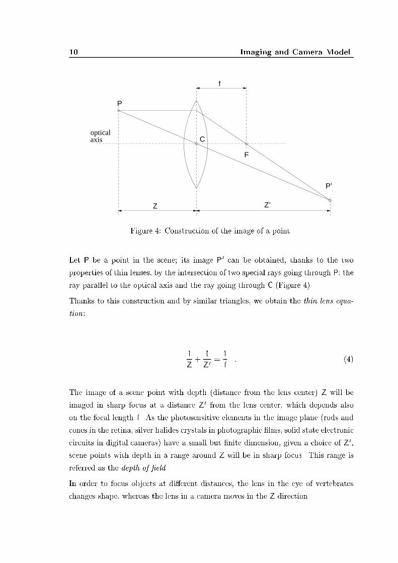
3.4 Epipolar geometry 31whose solution is the unit eigenvector corresponding to the smallest eigenvalue ofthe matrix L>L. SVD can be used also to solve this problem. Indeed, if L = UDV>is the SVD of L, then the solution is the column of V corresponding to the smallestsingular value of L.As in the case of calibration, a cause of inaccuracy in this linear method is thatthe value being minimized (jjLxjj) has no geometric meaning. A minimization ofa suitable cost function, like the error in the image plane, should be performed toachieve better accuracy [33, 64, 168]:� = jjm - ~Pwjj + jjm 0 - ~P 0w 0jj: (49)where w is the sought estimate of the coordinates of W. See [65] for a discussionabout algebraic versus geometric error minimization in gometric Computer Vision.3.4 Epipolar geometryLet us consider a stereo rig composed by two pinhole cameras (Figure 12). Let C1and C2 be the optical centers of the left and right cameras respectively. A 3-D pointW is projected onto both image planes, to points M1 and M2, which constitute aconjugate pair. Given a point M1 in the left image plane, its conjugate point in theright image is constrained to lie on a line called the epipolar line (of M1). Since M1may be the projection of an arbitrary point on its optical ray, the epipolar line is theprojection through C2 of the optical ray of M1. All the epipolar lines in one imageplane pass through a common point (E1 and E2 respectively.) called the epipole,which is the projection of the conjugate optical center.The fundamental matrixGiven two camera matrices, a world point of coordinates ~w1, is projected onto apair of conjugate points of coordinates ~m1 and ~m2:� ~m1 ' ~P1 ~w~m2 ' ~P2 ~w:

32 Structure from Stereo

R

R

W

M C

E

EM

C

1

1

22

2

2

1

1

Figure 12: Epipolar geometry. The epipole E1 of the �rst camera is the projectionof the optical center C2 of the second camera (and vice versa).The equation of the epipolar line of ~m1 can be easily obtained by projecting theoptical ray of ~m1 ~w = "c11 #+ �"Q-11 ~m10 # (50)with ~P2. From ~P2 " c11 # = ~P2 " -Q-11 ~q11 # = ~q2 -Q2Q-11 ~q1 = e2 (51)and ~P2 " Q-11 ~m10 # = Q2Q-11 ~m1 (52)we obtain the equation of the epipolar line of ~m1:~m2 = e2 + �Q2Q-11 ~m1: (53)

3.5 Recti�cation 33This is the equation of a line going through the points e2 (the epipole) andQ2Q-11 ~m1.The collinearity of these two points and ~m2 is expressed in the projective plane bythe triple product (see Appendix A):~m>2 (e2 ^Q2Q-11 ~m1) = 0; (54)which can be written in the more compact form~m>2 F ~m1 = 0; (55)by introducing the fundamental matrix F:F = [e2]^Q2Q-11 ; (56)where [e2]^ is a skew-symmetric matrix acting as the external product3 with e2.The fundamental matrix relates conjugate points; the role of left and right imagesis symmetrical, provided that we transpose F :~m>1 F> ~m2 = 0: (58)Since det([e2]^) = 0, the rank of F is in general 2. Moreover, F is de�ned up toa scale factor, because (55) is homogeneous. Hence it depends upon seven para-meters. Indeed, it can be parameterized with the epipolar transformation, that ischaracterized by the projective coordinates of the epipoles (2 � 2) and by the threecoe�cients of the homography (see Appendix A) between the two pencils of epipolarlines [93].3.5 Recti�cationGiven a pair of stereo images, recti�cation determines a transformation of eachimage plane such that pairs of conjugate epipolar lines become collinear and parallel3It is well-known that the external product t ^ x can be written as a matrix vector product[t]^x, with [t]^ = 24 0 -t3 t2t3 0 -t1-t2 t1 0 35 : (57)

34 Structure from Stereoto one of the image axes (usually the horizontal one). The recti�ed images can bethought of as acquired by a new stereo rig, obtained by rotating the original cameras.The important advantage of recti�cation is that computing correspondences is madesimpler. Other recti�cation algorithm can be found in [5, 60, 123, 112].When C1 is in the focal plane of the right camera, the right epipole is at in�nity,and the epipolar lines form a bundle of parallel lines in the right image. A veryspecial case is when both epipoles are at in�nity, that happens when the line C1C2(the baseline) is contained in both focal planes, i.e., the retinal planes are parallelto the baseline (see Figure 13). Epipolar lines then form a bundle of parallel linesin both images. Any pair of images can be transformed so that epipolar lines areparallel and horizontal in each image. This procedure is called recti�cation.

R

R

M

C

M

WC

2

2

11

1

2Figure 13: Recti�ed cameras. Image planes are coplanar and parallel to the baseline.3.5.1 Recti�cation of camera matricesWe will assume that the stereo rig is calibrated, i.e., the old PPMs ~Po1 and ~Po2 areknown. This assumption is not strictly necessary [60, 123], but leads to a simplertechnique. The idea behind recti�cation is to de�ne two new perspective matrices

3.5 Recti�cation 35~Pn1 and ~Pn2, that preserve the optical centers and with the baseline contained inthe focal planes. This ensures that epipoles are at in�nity, hence epipolar lines areparallel. In addition, to have a proper recti�cation, it is required that epipolar linesare horizontal, and that corresponding points have the same vertical coordinate. Wewill formalize analytically this requirements in Section 3.5.4, where we also show thatthe algorithm given in the present section satis�es that requirements.The new PPMs will have both the same orientation but di�erent position. Positions(optical centers) are the same as the old cameras, whereas orientation changes be-cause we rotate both cameras around the optical centers in such a way that focalplanes becomes coplanar and contain the baseline.In order to simplify the algorithm, the recti�ed PPMs will have also the same in-trinsic parameters. The resulting PPMs will di�er only in their optical centers. Thenew camera pair can be thought as a single camera translated along the X axis of itsstandard reference system. This intuitively satis�es the recti�cation requirements(formal proof in Section 3.5.4).Let us think of the new PPMs in terms of their factorization. From (36) and (33):~Pn1 = A[R j -R c1]; ~Pn2 = A[R j -R c2]: (59)The optical centers c1 and c2 are given by the old optical centers, computed with(32). The rotation matrixR is the same for both PPMs, and is computed as detailedbelow. The intrinsic parameters matrix A is also the same for both PPMs, but canbe chosen arbitrarily (see matlab code, Figure 14). We will specify R by means ofits row vectors R = 2664r>1r>2r>3 3775 (60)that are the X, Y and Z axes respectively, of the camera standard reference frame,expressed in world coordinates.According to the previous geometric arguments, we take:1. the new X axis parallel to the baseline: r1 = (c1 - c2)=jjc1 - c2jj2. the new Y axis orthogonal to X (mandatory) and to k: r2 = k^ r1

36 Structure from Stereo3. the new Z axis orthogonal to XY (mandatory) : r3 = r1 ^ r2where k is an arbitrary unit vector, that �xes the position of the new Y axis in theplane orthogonal to X. We take it equal to the Z unit vector of the old left matrix,thereby constraining the new Y axis to be orthogonal to both the new X and the oldleft Z. The algorithm is given in more details in the matlab version, Figure 14.3.5.2 The rectifying transformationIn order to rectify { let's say { the left image, we need to compute the trans-formation mapping the image plane of ~Po1 = [Qo1j~qo1] onto the image plane of~Pn1 = [Qn1j~qn1]. We will see that the sought transformation is the collinearitygiven by the 3 � 3 matrix T1 = Qn1Q-1o1 . The same result will apply to the rightimage.For any 3-D point w we can write� ~mo1 = ~Po1 ~w~mn1 = ~Pn1 ~w: (61)According to (35) , the equations of the optical rays are the following (since recti-�cation does not move the optical center)� w = c1 + �oQ-1o1 ~mo1w = c1 + �nQ-1n1 ~mn1; (62)Hence: ~mn1 = �Qn1Q-1o1 ~mo1: (63)where � is an arbitrary scale factor (it is an equality between homogeneous quant-ities). This is a clearer and more compact result than the one reported in [5].The transformation T1 is then applied to the original left image to produce therecti�ed image, as in Figure 17. Note that the pixels (integer-coordinate positions)of the recti�ed image correspond, in general, to non-integer positions on the originalimage plane. Therefore, the gray levels of the recti�ed image are computed bybilinear interpolation.

3.5 Recti�cation 37function [T1,T2,Pn1,Pn2] = rectify(Po1,Po2)% RECTIFY: compute rectification matrices in homogeneous coordinate%% [T1,T2,Pn1,Pn2] = rectify(Po1,Po2) computes the rectified% projection matrices "Pn1" and "Pn2", and the transformation% of the retinal plane "T1" and "T2" (in homogeneous coord.)% which perform rectification. The arguments are the two old% projection matrices "Po1" and "Po2".% Andrea Fusiello, MVL 1998 (fusiello@dimi.uniud.it)% factorize old PPMs[A1,R1,t1] = art(Po1);[A2,R2,t2] = art(Po1);% optical centers (unchanged)c1 = - inv(Po1(:,1:3))*Po1(:,4);c2 = - inv(Po2(:,1:3))*Po2(:,4);% new x axis (= direction of the baseline)v1 = (c1-c2);% new y axes (orthogonal to new x and old z)v2 = extp(R1(3,:)',v1);% new z axes (no choice, orthogonal to baseline and y)v3 = extp(v1,v2);% new extrinsic parameters (translation unchanged)R = [v1'/norm(v1)v2'/norm(v2)v3'/norm(v3)];% new intrinsic parameters (arbitrary)A = (A1 + A2)./2;A(1,2)=0; % no skew% new projection matricesPn1 = A * [R -R*c1 ];Pn2 = A * [R -R*c2 ];% rectifying image transformationT1 = Pn1(1:3,1:3)* inv(Po1(1:3,1:3));T2 = Pn2(1:3,1:3)* inv(Po2(1:3,1:3));------------------------function [A,R,t] = art(P)% ART: factorize a PPM as P=A*[R;t]Q = inv(P(1:3, 1:3));[U,B] = qr(Q);R = inv(U);t = B*P(1:3,4);A = inv(B);A = A ./A(3,3);Figure 14: Working matlab code of the rectify function.

38 Structure from Stereo3.5.3 Summary of the Rectification algorithmThe Rectification algorithm can be summarized as follows:� Given a stereo pair of images I1,I2 and PPMs Po1,Po2 (obtained by calib-ration);� compute [T1,T2,Pn1,Pn2] = rectify(Po1,Po2) (see box);� rectify images by applying T1 and T2.Reconstruction of 3-D position can be performed from the recti�ed images directly,using Pn1,Pn2.The code of the algorithm, shown in Figure 14 is simple and compact, and thecomments enclosed make it understandable without knowledge of matlab.3.5.4 Recti�cation analysisIn this section we will (i) formulate analytically the recti�cation requirements, and(ii) prove that our algorithm yields PPMs ~Pn1 and ~Pn2 that satis�es such require-ments.Definition 3.1A pair of PPMs ~Pn1 and ~Pn2 are said to be recti�ed if, for any pointm1 = (u1; v1)>in the left image, its epipolar line in the right image has equation v2 = v1, and, forany point m2 = (u2; v2)> in the right image, its epipolar line in the left image hasequation v1 = v2.In the following, we shall write ~Pn1 and ~Pn2 as follows:~Pn1 = 2664 s>1 s14s>2 s24s>3 s34 3775 = [Sj~s] ~Pn2 = 2664 d>1 d14d>2 d24d>3 d34 3775 = [Dj~d]: (64)

3.5 Recti�cation 39Proposition 3.2Two perspective projection matrices ~Pn1 and ~Pn2 are recti�ed if and only if8>><>>: s1c2 + s14 6= 0s2c2 + s24 = 0s3c2 + s34 = 0 and 8>><>>: d1c1 + d14 6= 0d2c1 + d24 = 0d3c1 + d34 = 0 (65)and s2w + s24s3w + s34 = d2w + d24d3w + d34 ; (66)where ~Pn1 and ~Pn2 are written as in (64) and c1 and c2 are the respective opticalcenter's coordinates.Proof As we know, the epipolar line of ~m2 is the projection of its optical ray ontothe left camera, hence its parametric equation writes:~m1 = ~Pn1 "c21 #+ ~Pn1 "�D-1 ~m20 # = ~e1 + �SD-1 ~m2 (67)where ~e1, the epipole, is the projection of the conjugate optical center c2: 4~e1 = ~Pn1 " c21 # = 2664 s1c2 + s14s2c2 + s24s3c2 + s34 3775 : (68)The parametric equation of the epipolar line of ~m2 in image coordinates becomes:8>><>>:u = [m1]1 = [~e1]1 + �[~n]1[~e1]3 + �[~n]3v = [m1]2 = [~e1]2 + �[~n]2[~e1]3 + �[~n]3 (69)where ~n = SD-1 ~m2; and [:]i is the projection operator extracting the ith componentfrom a vector.Analytically, the direction of each epipolar line can be obtained by taking the de-rivative of the parametric equations (69) with respect to �:4In this section only, to improve readability, we omit the transpose sign in scalar products. Allvector products are scalar products, unless otherwise noted.

40 Structure from Stereo8>><>>: dud� = [~n]1[~e1]3 - [~n]3[~e1]1([~e1]3 + �[~n]3)2dvd� = [~n]2[~e1]3 - [~n]3[~e1]2([~e1]3 + �[~n]3)2 : (70)Note that the denominator is the same in both components, hence it does not a�ectthe direction of the vector. The epipole is rejected to in�nity when [~e1]3 = 0. Inthis case, the direction of the epipolar lines in the right image doesn't depend on nand all the epipolar lines becomes parallel to vector [[~e1]1 [~e1]2]> . The same holds,mutatis mutandis, for the left image.Hence, epipolar lines are horizontal if and only if (65) holds. The vertical coordinateof conjugate points is the same in both image if and only if (66) holds, as can easilyseen by plugging (64) into (30). �Proposition 3.3The two camera matrices ~Pn1 and ~Pn2 produced by the Rectification algorithmare recti�ed.Proof We shall prove that, if ~Pn1 and ~Pn2 are built according to the Rectifica-tion algorithm, then (65) and (66) hold.From (59) we obtains14 = -s1c1 d14 = -d1c2 s1 = d1s24 = -s2c1 d24 = -d2c2 s2 = d2s34 = -s3c1 d34 = -d3c2 s3 = d3 (71)From the factorization (36), assuming = 0, we obtain2664s>1s>2s>3 3775 = AR = 2664�ur>1 + u0r>3�vr>2 + v0r>3r>3 3775 (72)From the construction of R, we have that r1, r2 and r3 are mutually orthogonal andr1 = �(c1 - c2) with � = 1=jjc1 - c2jj.

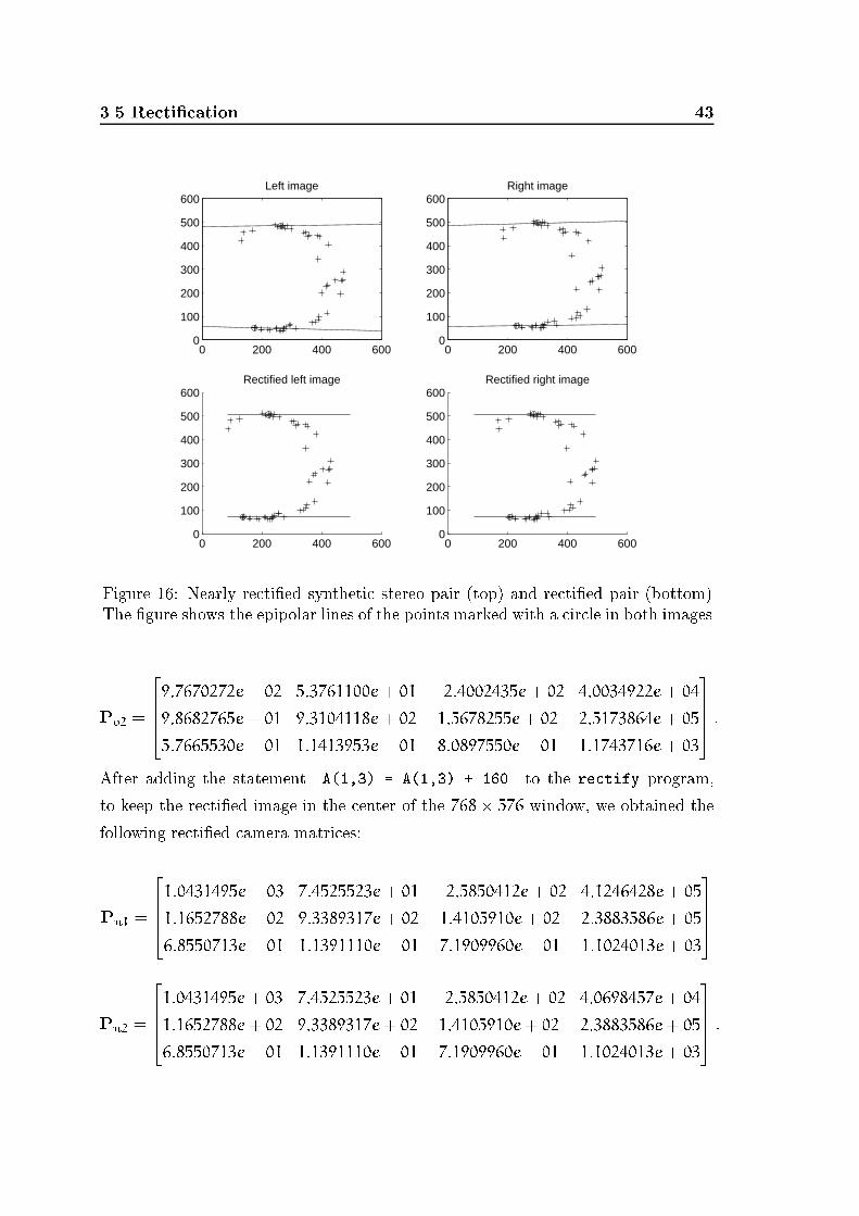
3.5 Recti�cation 41From all these facts, the following four identity are derived:s1(c1 - c2) =�s1r1 = �(�ur1 + u0r3)r1 = �(�ur1r1 + u0r3r1) = ��u 6= 0(73)s2(c1 - c2) =�s2r1 = �(�vr2 + v0r3)r1 = �(�vr2r1 + v0r3r1) = 0 (74)s3(c1 - c2) =�s3r1 = �r3r1 = 0 (75)s2 ^ s3 = s2 ^ r3 = �(r2 ^ r3) = �r1 (76)The parameter � in (76) is scalar taking into account that s2 is a linear combinationof r2 and r3.Equation (65) follows easily from (73) (74)(75). Equation (66) is equivalent to(s2w + s24)(d3w + d34) = (s3w + s34)(d2w + d24): (77)Expanding, and using (74),(76) and properties of the external product we obtain-s2(c1 - c2)s3w + (s2c1)(s3c2) - (s2c2)(s3c1) =(s2c1)(s3c2) - (s2c2)(s3c1) =(s2 ^ s3)(c1 ^ c2) =�r1(c1 ^ c2) =��(c1 - c2)(c1 ^ c2) = 0: (78)�3.5.5 Experimental resultsWe ran tests to verify that the algorithm performed recti�cation correctly, andalso to check that the accuracy of the 3-D reconstruction did not decrease whenperformed from the recti�ed images directly.CorrectnessThe tests used both synthetic and real data. Each set of synthetic data consistedof a cloud of 3-D points and a pair of PPMs. For reasons of space, we reportonly two examples. Figure 16 shows the original and recti�ed images with a nearlyrecti�ed stereo rig: the camera translation was -[100 2 3] mm and the rotationangles roll=1:5o, pitch=2o, yaw=1o. Figure 15 shows the same with a more general

42 Structure from Stereo

−400 −200 0 200 400−200

0

200

400

600Left image

−400 −200 0 200 400−200

0

200

400

600Right image

−1000 −500 0−200

0

200

400

600

800Rectified left image

−1000 −500 0−200

0

200

400

600

800Rectified right image

Figure 15: General synthetic stereo pair (top) and recti�ed pair (bottom). The�gure shows the epipolar lines of the points marked with a circle in both images.geometry: the camera translation was -[100 20 30] mm and the rotation anglesroll=19o pitch=32o and yaw=5o.Real-data experiments used calibrated stereo pairs, courtesy of INRIA-Syntim. Weshow the results obtained with a nearly recti�ed stereo rig (Figure 17) and with amore general stereo geometry (Figure 18). The right image of each pair shows threeepipolar lines corresponding to the points marked by a cross in the left image. Thepixel coordinates of the recti�ed images are not constrained to lie in any specialpart of the image plane, and an arbitrary translation were applied to both images tobring them in a suitable region of the plane; then the output images were croppedto the size of the input images. In the case of the \Sport" stereo pair (image size768� 576), we started from the following camera matrices:Po1 = 26649:7655352e+ 02 5:3829220e+ 01 -2:3984731e+ 02 3:8754954e+ 059:8498581e+ 01 9:3334472e+ 02 1:5747888e+ 02 2:4287923e+ 055:7902862e- 01 1:1085118e- 01 8:0773700e- 01 1:1185149e+ 033775

3.5 Recti�cation 43

0 200 400 6000

100

200

300

400

500

600Left image

0 200 400 6000

100

200

300

400

500

600Right image

0 200 400 6000

100

200

300

400

500

600Rectified left image

0 200 400 6000

100

200

300

400

500

600Rectified right image

Figure 16: Nearly recti�ed synthetic stereo pair (top) and recti�ed pair (bottom).The �gure shows the epipolar lines of the points marked with a circle in both images.Po2 = 26649:7670272e+ 02 5:3761100e+ 01 -2:4002435e+ 02 4:0034922e+ 049:8682765e+ 01 9:3104118e+ 02 1:5678255e+ 02 2:5173864e+ 055:7665530e- 01 1:1413953e- 01 8:0897550e- 01 1:1743716e+ 033775 :After adding the statement A(1,3) = A(1,3) + 160 to the rectify program,to keep the recti�ed image in the center of the 768� 576 window, we obtained thefollowing recti�ed camera matrices:Pn1 = 26641:0431495e+ 03 7:4525523e+ 01 -2:5850412e+ 02 4:1246428e+ 051:1652788e+ 02 9:3389317e+ 02 1:4105910e+ 02 2:3883586e+ 056:8550713e- 01 1:1391110e- 01 7:1909960e- 01 1:1024013e+ 033775Pn2 = 26641:0431495e+ 03 7:4525523e+ 01 -2:5850412e+ 02 4:0698457e+ 041:1652788e+ 02 9:3389317e+ 02 1:4105910e+ 02 2:3883586e+ 056:8550713e- 01 1:1391110e- 01 7:1909960e- 01 1:1024013e+ 033775 :

44 Structure from Stereo

Left image Right image

Rectified left image Rectified right image

Figure 17: \Sport" stereo pair (top) and recti�ed pair (bottom). The right picturesplot the epipolar lines corresponding to the points marked in the left pictures.

3.5 Recti�cation 45Left image Right image

Rectified left image Rectified right image

Figure 18: \Color" stereo pair (top) and recti�ed pair (bottom). The right picturesplot the epipolar lines corresponding to the points marked in the left pictures.

46 Structure from StereoAccuracyIn order to evaluate the errors introduced by recti�cation on reconstruction, wecompared the accuracy of 3-D reconstruction computed from original and recti�edimages. We used synthetic, noisy images of random clouds of 3-D points. Imagingerrors were simulated by perturbing the image coordinates, and calibration errorsby perturbing the intrinsic and extrinsic parameters, both with additive, Gaussiannoise. Reconstruction were performed using the Linear-Eigen method, described inSection 3.3.

0 0.005 0.01 0.015 0.02 0.025 0.03 0.035 0.04 0.045 0.050

0.2

0.4

0.6

0.8

1

1.2

std dev of relative error on image points position

aver

age

rela

tive

erro

r on

3d

poi

nts

posi

tion

0 0.005 0.01 0.015 0.02 0.025 0.03 0.035 0.04 0.045 0.050

0.1

0.2

0.3

0.4

0.5

0.6

0.7

0.8

0.9

std dev of relative error on calibration parameters

aver

age

rela

tive

erro

r on

3d

poi

nts

posi

tion

Figure 19: Reconstruction error vs noise levels in the image coordinates (left) andcalibration parameters (right) for the general synthetic stereo pair. Crosses referto reconstruction from recti�ed images, circles to reconstruction from unrecti�edimages.

0 0.005 0.01 0.015 0.02 0.025 0.03 0.035 0.04 0.045 0.050

0.2

0.4

0.6

0.8

1

1.2

std dev of relative error on image points position

aver

age

rela

tive

erro

r on

3d

poi

nts

posi

tion

0 0.005 0.01 0.015 0.02 0.025 0.03 0.035 0.04 0.045 0.050

0.1

0.2

0.3

0.4

0.5

0.6

0.7

0.8

std dev of relative error on calibration parameters

aver

age

rela

tive

erro

r on

3d

poi

nts

posi

tion

Figure 20: Reconstruction error vs noise levels in the image coordinates (left) andcalibration parameters (right) for the nearly recti�ed synthetic stereo pair. Crossesrefer to reconstruction from recti�ed images, circles to reconstruction from unrecti-�ed images.

3.6 Conclusions 47Figures 19 and 20 show the average (over the set of points) relative error measured on3-D point position, plotted against noise. Figure 19 shows the results for the stereorig used in Figure 15, and Figure 20 for the one used in Figure 16. Each point plottedis an average over 100 independent trials. The abscissa is the standard deviation ofthe relative error on coordinates of image point or calibration parameters.3.6 ConclusionsGiven two images and a set of matched points, the 3-D coordinates of the corres-ponding world points can be reconstructed with a simple linear technique, if cameraparameters (intrinsic and extrinsic) are known. The process of measuring cam-era parameters is called calibration. Epipolar geometry relates a point in one imagewith the set of possible matches in the other, which constitutes a line, called epipolarline. Matching is greatly simpli�ed if the epipolar lines are parallel and horizontalin each image, i.e., if the images are recti�ed. In this chapter we have developed asimple and compact recti�cation algorithm. The correct behavior of the algorithmhas been demonstrated with both synthetic and real images. Interestingly enough,reconstruction can be performed directly from the disparities of the recti�ed images,using the rectifying PPMs. Our tests show that this process does not introducesappreciable errors compared with reconstructing from the original images.

Chapter 4Stereo MatchingIn the previous chapter we assumed that we could identify conjugate pairs, thatis to say, pairs of points in the two images that are projection of the same pointsin the scene. In this chapter we will address the problem of detecting conjugatepairs in stereo images. We propose a novel stereo matching algorithm, called SMW(Symmetric Multi-Window) addressing robust disparity estimation in the presenceof occlusions. The algorithm is an adaptive, multi-window scheme using left-rightconsistency to compute disparity and its associated uncertainty. We demonstrateand discuss performances with both synthetic and real stereo pairs, and show howour results improve on those of closely related techniques for both accuracy ande�ciency.4.1 IntroductionDetecting conjugate pairs in stereo images is a challenging problem known as thecorrespondence problem, i.e., �nding which points in the left and right images areprojections of the same scene point (a conjugate pair).Several factors make the correspondence problem di�cult: (i) its inherent ambiguity,which requires the introduction of physical and geometric constraints; (ii)occlusions;(iii) photometric distortions and (iv) �gural distortion. In Section 4.2 these factorsare described, and the available constraints are introduced. Then, the existingmethods are outlined.In Section 4.3 we present a new Symmetric, Multi-Window algorithm (henceforth49

50 Stereo MatchingSMW) for stereo matching, which addresses the problem mentioned in Section 4.1,and outperforms closely related methods. SMW's assumptions are clearly stated inSection 4.3.1. SMW is based on the Block Matching algorithm (Section 4.3.2); itemploys an adaptive, multi-window scheme to cure distortions and yield accuratedisparities (Section 4.3.3), associated to uncertainty estimates. Robustness in thepresence of occlusions is achieved thanks to the left-right consistency constraint (Sec-tion 4.3.4). A consistent uncertainty estimation mechanism (Section 4.3.5) guaran-tees that the depth maps produced can be used by data fusion schemes like [148]. InSection 4.3.6 we give a pseudo-code summary of the SMW algorithm. A detailed ex-perimental evaluation, including a comparison with similar methods reported in theliterature, is reported in Section 4.4. Our results (stereo pairs and disparity maps)are available on the web (http://www.dimi.uniud.it/~fusiello/demo-smw/smw.html)where the source code for the SMW algorithm can be downloaded as well.4.2 The correspondence problemThe correspondence problem (or matching problem) can be regarded as a searchproblem, since for each element on the left image (a point, region, or generic feature),a similar element is to be found in the right one, according to a given similaritymeasure. The output of a stereo matching algorithm is a set of correspondences, ora disparity map that gives the disparity for some or all points of a reference image.To prevent ambiguous or false matches and avoid combinatorial explosion, thesearch space must be suitably constrained. Geometric, physical and photometricconstraints imposed by both the observer (our stereo rig) and the scene, include thefollowing.Similarity constraint [51]. Left and right images of a given scene element aresimilar. This is often implicit.Epipolar constraint (see Chapter 3). Given a point in the left image, the cor-responding point must lie on a straight line (called epipolar line) in the rightimage. This constraint reduces the search space from two-dimensional to one-dimensional. It applies in every situation, provided that the epipolar geometryis known.

4.2 The correspondence problem 51Smoothness constraint [96]. The distance of scene points from the cameraschanges smoothly almost everywhere, thereby limiting the allowable disparitygradient. This fails, obviously, at depth discontinuities.Uniqueness constraint [96]. Each image element has one and only one conjugate.This fails if transparent objects are presents or in the presence of occlusions.Ordering constraint [7]. If point m1 in the one image matches point m 01 in theother image, then the corresponding of a pointm2 that lies at the right (left) ofm1 must lie at the right (left) ofm 01. This constraint hold for points belongingon the surface of an opaque object. It fails at region known as forbidden zone(See Figure 21).

2

1m

P2

m

Q

P1

12

m’m’Figure 21: Ordering constraint. Point Q , which lies behind an opaque object,violates the ordering constraint. The shaded region is the forbidden zone of P1.Major problems a�ecting machine stereo arise because the scene is viewed from twodi�erent viewpoints, which is also the key feature of stereo. The larger the baselinethe more severe these e�ects, which include the following.

52 Stereo MatchingOcclusions. Since the two images of the scene are slightly di�erent, there are ele-ments that are imaged only in one camera. Hence, there are image pointswithout a corresponding, or, stated in other words, not all points in one imagebelongs to a conjugate pair.Photometric distortion. A typical assumption is that the perceived intensity ofa surface patch does not depend on the viewing direction: light source is apoint at in�nity and the surfaces are Lambertian (see Chapter 2). This is nottrue in general, and the same world point takes di�erent intensities in eachview.Figural distortion. Owing to perspective projection, the same object appears dif-ferent when projected in the left and right images.4.2.1 Matching techniquesThe techniques adopted for the stereo matching problem can be classi�ed along twodimensions: the kind of image element considered for matching (What to match),and the techniques to compute matching (How to match). In addition, one can beinterested in the computational schemes adopted, especially when biological plaus-ibility is of concern [15] .What to matchLet us address the �rst issue. Some algorithms [26, 96] match individual pixels,i.e., the atomic elements in an image. More robust methods, called area-based ,perform matching between gray levels of image patches (windows), by computingsome form of similarity or correlation. The disparity may then be computed forevery pixel [35, 41], for the centers of the windows [90, 162], or for selected pointsof interest [56].Since gray-levels are not identical in the two image, some problems arise with match-ing raw intensities. They can be overcome by considering the output of a bandpass�lter, usually a Laplacian of Gaussian (LoG) �lter [108]. One could also computethe response of a bank of �lters at a given image point, which de�nes a vector char-acterizing the local structure of the image [78, 157]. A similar vector is estimated

4.2 The correspondence problem 53on the other image, in order to compute matching.Matching image features is generally more robust; the related class of algorithms iscalled feature-based . In the present context, the term \features" indicates physicallymeaningful cues, such as edges [97, 52, 116, 7, 110], segments (collinear connectededges) [102], and corners (where two edges cross) [8]. Features can be extracted bybandpass �lters, derivative operators or ad hoc non-linear operators.The local phase of the image signal { computed via Fourier or Gabor transforms {has also been used for matching [77, 76, 67]. As disparity should be less than onepixel to avoid aliasing (according to the sampling theorem, or the \quarter cyclelimit" [96]), a multi-resolution scheme should be employed.How to matchWe now come to the second question: Once chosen the elements to be matched, howto perform matching?Correlation techniques consist in �nding the amount of shifting that yields themaximum similarity score between the left and the right elements. Although severalcorrelation measures have been proposed, the Sum of Squared Di�erences (SSD)measure is regarded as a reasonable choice [2, 41, 35, 111, 74, 79, 47]. Recently,anew approach based the local ordering of intensities have been presented [163] withpromising results.With relaxation-based methods the elements are joined by weighted links; the initialweights are iteratively updated by propagating constraints, until some equilibriumcon�guration is reached [96, 97, 52, 116, 8].Dynamic programming techniques adopt a cost function, that embeds the constraintsand is minimized to get the best set of matches [110, 7, 74, 47, 11, 26]. The solutionis a curve in the match space [26, 47] or the disparity space [74]. Usually, the costfunctional is derived using Bayesian reasoning [47, 11, 26].A novel approach to matching consists in representing image scan lines by means ofintrinsic curves [139], i.e, the paths followed by a descriptor vector as the scan lineis traversed from left to right. Intrinsic curves are invariant to image displacements,and this property is exploited to compute matching.

54 Stereo MatchingComputational schemesAs far as the computational scheme is concerned, algorithms can be classi�ed intocooperative, coarse-to-�ne and feed-forward (see [15] for more details).Cooperative models, pioneered by Marr and Poggio [96], exploit the properties ofrecurrent nets, which perform relaxation to a minimum energy con�guration.In coarse-to-�ne models, the disparities computed at di�erent spatial scales are fusedto compute the �nal disparity estimate. In biological vision, coarse-to-�ne modelsidentify a special class of algorithms using multiple spatial �lters that simulate re-ceptive �elds [97, 108]. In machine vision, this paradigm is applicable to any scheme,in order to get scale independence and data redundancy [84]. It is mandatory onlywith phase-based methods.Whereas the cooperative and the coarse-to-�ne techniques require cooperative feed-back or sequential disparity processing over the spatial scales, the feed-forwardscheme [162] operates in one shot, like most of the machine stereo algorithms.For further details on machine stereo, the reader can consult the book [53] or thesurveys in [16, 30]; a review on human computational stereo is given in [15].4.3 A new area-based stereo algorithmIn this section we present our new, e�cient stereo algorithm addressing robust dis-parity estimation in the presence of occlusions. The algorithm is an adaptive, multi-window scheme using left-right consistency to compute disparity and its associateduncertainty.4.3.1 AssumptionsWith no loss of generality, we assume that conjugate pairs lie along raster lines, thatis, the stereo pair has been recti�ed (Section 3.5) to achieve parallel and horizontalepipolar lines in each image.We also assume that the image intensities I(x; y) of corresponding points in thetwo images are the same. If this is not true, the images can be normalized by asimple algorithm [26] that computes the parameters �; � of the gray-level global

4.3 A new area-based stereo algorithm 55transformation Il(x; y) = �Ir(x; y) + � 8(x; y)by �tting a straight line to the plot of the left cumulative histogram versus the rightcumulative histogram. This normalization fails if images are taken from viewpointstoo far apart.

0 50 100 150 200 250 3000

50

100

150

200

250

300

Figure 22: Ten percentile points from \Shrub" histograms.4.3.2 The Block Matching algorithmThe basic structure of the block matching algorithm can be outlined as follows.For each pixel in the image chosen as reference (e.g., the left one, Il), similarityscores are computed by comparing a �xed, small window centered on the pixel toa window in the other image (here, Ir), shifting along the raster line. Windowsare compared through the normalized SSD measure, that quanti�es the di�erencebetween intensity patterns:C(x; y; d) = X(�;�)[Il(x+�; y+�) - Ir(x+�+ d; y+�)]2sX(�;�) Il(x+�; y+�)2X(�;�) Ir(x+�+d; y+�)2 (79)

56 Stereo Matching

Figure 23: E�cient implementation of correlation.where � 2 [-n; n]; � 2 [-m;m]. The disparity estimate for pixel (x; y) is the onethat minimizes the SSD error:do(x; y) = argmind C(x; y; d): (80)Sub-pixel accuracy can be achieved, for instance, by �tting a parabola to the SSDerror function C(d) in the neighborhood of the minimum d0 [2]:s(x; y) = 12 C(x; y; do-1) - C(x; y; do+1)C(x; y; do-1)-2C(x; y; do)+C(x; y; do+1) (81)The Simple Block Matching (henceforth SBM) algorithm is reported here.Algorithm 1 SBMlet Ir, Il the right and left N�N images;let W a n� n window (with n� N);for each pixel Il(x; y)for each disparity d = (dx; dy) in some rangeC(x; y;d) = X(�;�)2W[Il(x+ �; y+ �) - Ir(x + �- dx; y+ �- dy)]2;enddl(x; y) argmindC(x; y;d)endend

4.3 A new area-based stereo algorithm 57

jumpDepth

Fixed Multiple Window Windows

Figure 24: Multiple windows approach. If one use windows of �xed size with di�erentcenters, it is likely that one of them will cover a constant depth area.SBM has an asymptotic complexity of O(N2nm), with N the image size. However,we can observe that squared di�erences need to be computed only once for eachdisparity, and the sum over the window needs not be recomputed from scratch whenthe window moves by one pixel (see Figure 23). The optimized implementation thatfollows from this observation [35] has a computational complexity of O(4N2), thatis independent of the window size.4.3.3 The need for multiple windowsAs observed by Kanade and Okutomi [79], when the correlation window covers aregion with non-constant disparity, area-based matching is likely to fail, and theerror in the depth estimates grows with the window size. Reducing the latter, onthe other hand, makes the estimated disparities more sensitive to noise.Figure 25: The nine correlation windows. The pixel for which disparity is computedis highlighted.To overcome such di�culties, Kanade and Okutomi proposed a statistically sound,adaptive technique which selects at each pixel the window size that minimizes the

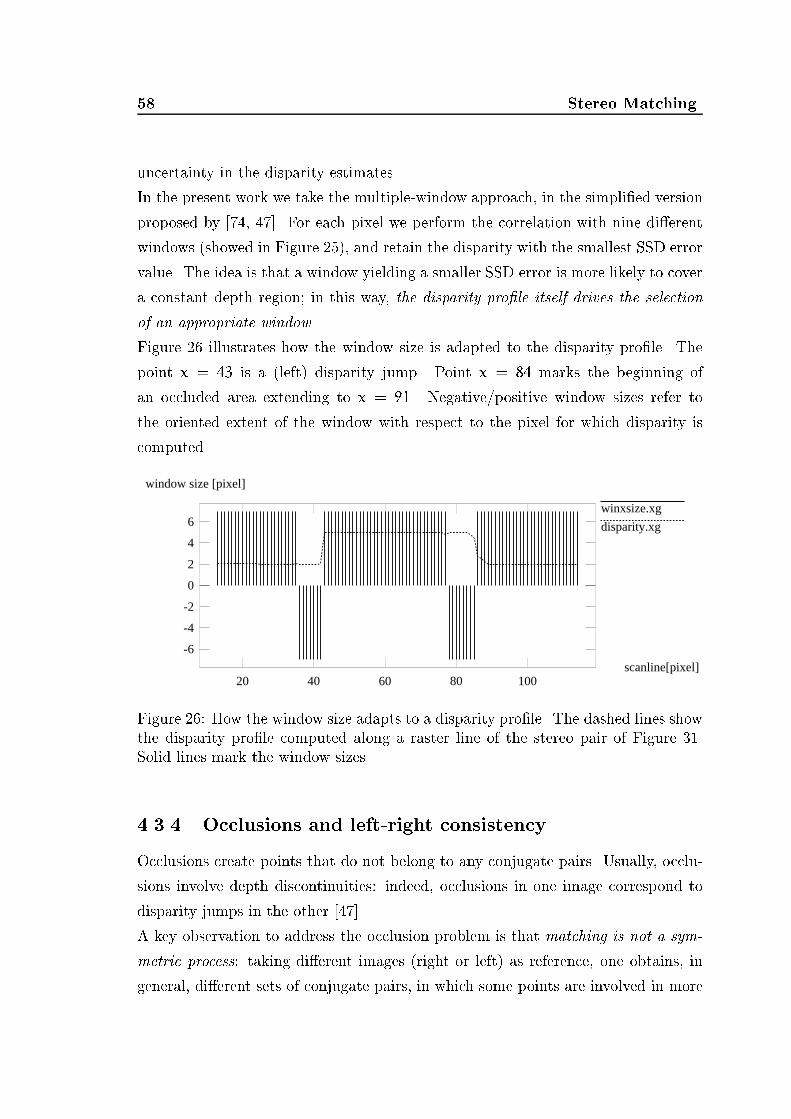
58 Stereo Matchinguncertainty in the disparity estimates.In the present work we take the multiple-window approach, in the simpli�ed versionproposed by [74, 47]. For each pixel we perform the correlation with nine di�erentwindows (showed in Figure 25), and retain the disparity with the smallest SSD errorvalue. The idea is that a window yielding a smaller SSD error is more likely to covera constant depth region; in this way, the disparity pro�le itself drives the selectionof an appropriate window.Figure 26 illustrates how the window size is adapted to the disparity pro�le. Thepoint x = 43 is a (left) disparity jump. Point x = 84 marks the beginning ofan occluded area extending to x = 91. Negative/positive window sizes refer tothe oriented extent of the window with respect to the pixel for which disparity iscomputed.

winxsize.xg

disparity.xg

window size [pixel]

scanline[pixel]

-6

-4

-2

0

2

4

6

20 40 60 80 100Figure 26: How the window size adapts to a disparity pro�le. The dashed lines showthe disparity pro�le computed along a raster line of the stereo pair of Figure 31.Solid lines mark the window sizes.4.3.4 Occlusions and left-right consistencyOcclusions create points that do not belong to any conjugate pairs. Usually, occlu-sions involve depth discontinuities: indeed, occlusions in one image correspond todisparity jumps in the other [47].A key observation to address the occlusion problem is that matching is not a sym-metric process: taking di�erent images (right or left) as reference, one obtains, ingeneral, di�erent sets of conjugate pairs, in which some points are involved in more

4.3 A new area-based stereo algorithm 59than one conjugate pairs. Such pairs are not invariant to the choice of the referenceimage. As each point in one image can have at most one corresponding point inthe other (the uniqueness constraint), such pairs can be discarded (left-right con-sistency) [41, 35].IIl r

AB C

A’C’

Figure 27: Left-right consistency. Matching left to right, point A is correctlymatched to A 0. Point B is incorrectly given C 0 as a match, but C 0 matches actuallyC 6= B.Consider for instance point B of Figure 27 and take the left image, Il, as reference.Although B has no corresponding point in the right image, Il (its conjugate pointis occluded), the SSD minimization returns a match anyhow ( C 0). If Ir is taken asreference, instead, C 0 is correctly matched to its conjugate point (C) in the left image.Therefore the conjugate pairs (B;C 0) and (C;C 0) violate left-right consistency; inother words, C 0 does not satisfy the uniqueness constraint. Notice that the (C 0;C)pair allow us to recognize that point B is occluded (strictly speaking, its conjugatepoint is occluded); our approach takes advantage of left-right consistency to detectocclusions and suppress the resulting infeasible matches.For each point (x; y) in the left image, the disparity dl(x; y) is computed as describedin Section 4.3.2. The process is repeated with the right image as reference.If dl(x; y) = -dr(x + dl(x; y); y) the point is assigned the computed disparity;otherwise it is marked as occluded and a disparity is assigned heuristically. Following[85], we assume that occluded areas, occurring between two planes at di�erent depth,take the disparity of the deeper plane.It should be said that, in presence of large amount of noise or distortion, the left-right consistency could fail for true conjugate pairs, and points could be wronglymarked as occluded. A simple non-linear �ltering of the occlusions map (a binaryimage showing only occluded points) would discard those \outliers".

60 Stereo Matching4.3.5 Uncertainty estimatesArea-based algorithms are likely to fail not only in occluded regions, but also inpoorly textured regions, which make disparity estimates more uncertain; it is there-fore essential to assign con�dence estimates to disparities. Several uncertainty es-timation schemes have been proposed for SSD, mostly based on the shape of theSSD error function [2, 148].Our approach takes advantage of the multiple windows. Disparity estimation issensitive to window shape in two cases: �rst, near a disparity jump (as discussedin Section 4.3.3) and, second, where the texture is poor, or the signal-to-noise ratio(SNR) is low. Consequently, we de�ne uncertainty as the estimated variance of thedisparity measures obtained with the various windows (see algorithm summary innext section); occluded points are assigned in�nite variance. Experimental resultsshow that such an uncertainty measure is consistent, i.e., it grows as the SNRdecreases (Section 4.4).4.3.6 Summary of the SMW algorithmWe summarize our algorithm, called SMW (for Symmetric Multi-Window) in pseudo-code. Let C(x; y; d; Il; Ir; w) be the SSD error computed from Il to Ir according to(79) at point (x; y), with disparity d and window w. Let sl be the sub-pixel correc-tion de�ned by (81). The y coordinate is omitted for the sake of simplicity, sincewe assume horizontal epipolar lines.Algorithm 2 SMWlet Ir, Il the right and left N�N images;for all (x; y) in the left image Il dofor all windows w = 1 : : :K dodl;w(x) argmind C(x; y; d; Il; Ir; w)dr;w(x) argmindC(x; y; d; Ir; Il; w)end�2d(x) = 1K-1PKw=1(dl;w(x) - �dl;w(x))2:dl(x) argminwC(x; y; dl;w; Il; Ir; w)

4.4 Experimental results 61dr(x) argminw C(x; y; dr;w; Ir; Il; w)d(x) dl(x) + subpixell(x)endfor all (x; y) in Il doif (dl(x) 6= -dr(x+ dl(x)) then �2d(x) +1endendIt is worth noting that the only one SSD value per pixel needs to be computed.Indeed, each o�-centered windows for a pixel is the on-centered window for anotherpixel.4.4 Experimental resultsThis section reports the main results of experimental evaluation of SMW. The eval-uation was aimed at assessing� the accuracy of disparity computation,� robustness against occlusion,� the consistency of uncertainty estimation,� the performance of SMW when compared to similar algorithms.

Figure 28: Square RDS. The right imageof the stereogram is computed by warp-ing the left one, which is a random tex-ture (left), according to a given disparitypattern (right): the square has disparity10 pixel, the background 3 pixel.Figure 29: Computed disparity mapby SBM for the square RDS with 3�3window (left) and 7�7 window (right);MAE is 0.240 and 0.144, respectively.

62 Stereo MatchingWe used synthetic data sets commonly found in the stereo literature and controlledamounts of noise. We also reproduced patterns used for testing algorithms used inour comparative evaluation. The next section reports the results as well as furthertests with real stereo pairs of size 128� 128.4.4.1 Random-dot stereogramsWe �rst performed experiments on noise-free random-dot stereograms (RDS), shownin Figure 28. In the disparity maps, displayed as images, the gray level encodes thedisparity, that is the depth (the brighter the closer); images have been equalized toimprove readability; sub-pixel accuracy values have been rounded to integers. Theestimated Mean Absolute Error (MAE), that is the mean of absolute di�erencesbetween estimated and ground true disparities, has been computed as a performanceindex.

Figure 30: Computed disparity map (left) and uncertainty (right) by SMW forthe square RDS (top) and for the circle RDS (bottom). MAE is 0.019 and 0.026.respectively.The results of SBM applied to the random-dot stereogram of Figure 28 shows howmost of the problems outlined in Sections 4.3.3 and 4.3.4 a�ect disparity computa-tion. Figure 29 shows the disparity maps computed by SBM with �xed windows3�3 and 7�7. Both pictures show the e�ect of disparity jumps (near the left and

4.4 Experimental results 63

0 5 10 15 20 25 30 35 40 45 500

0.5

1

1.5

2

2.5

noise std deviation

MA

E

SSD

SMW

−15 −10 −5 0 5 10 15 200

0.1

0.2

0.3

0.4

0.5

0.6

0.7

0.8

0.9

signal to noise ratio [db]

disp

arity

unc

erta

inty

Figure 31: MAE of SMW and SBM vsnoise standard deviation for the squareRDS. Window is 7�7. Figure 32: Mean uncertainty vs SNR fora constant disparity region of the squareRDS.horizontal borders of the square patch) and of occlusions (near the right border ofthe square patch). The SMW algorithm with a 7 � 7 window was applied to thesquare RDS of Figure 28 and to a circular RDS (not shown here). Figure 30 showthe disparity maps computed by SMW and the estimated uncertainty maps (thedarker the lower) in both cases.The MAE is negligible, and may be ascribed to sub-pixel estimation only. Theoccluded points, shown in white in the uncertainty maps, are identi�ed with 100%accuracy in both cases. The circle RDS shows that the algorithm is not biasedtoward square disparity patterns, as the shape of the SSD windows might suggest.The reader could compare the present results to those reported in [26].Experiments with various noisy RDSs show a graceful degradation when noise in-creases. Gaussian noise with zero mean and increasing variance was added inde-pendently to both images of the square RDS. Figure 31 plots the MAE against thestandard deviation of the noise for SMW and SBM. Each point depicts the averageresult of 20 independent trials. Images were 8-bit deep, monochrome.In order to assess the uncertainty estimator incorporated in SMW, we plotted theaverage uncertainty computed over a square patch of uniform disparity against theSNR, de�ned as SNR = 10 log10 Image varianceNoise variance : (82)

64 Stereo MatchingThe results (Figure 32) show that the computed uncertainty consistently increasesas the SNR decreases.4.4.2 Gray-level rampWe performed a systematic, quantitative comparison between SMW, our implement-ation of the Adaptive Window (AW) algorithm [79] (perhaps the closest method toSMW in the literature), and SBM with di�erent window sizes. The evaluation wasbased on the main test pattern used by [79]: an input stereo pair of an intensityramp in the horizontal direction, warped according to a given disparity pattern.The left disparity jump creates a \disocclusion" area that is �lled with random dots(Figure 33). Gaussian noise with zero mean and unit variance (gray level) was addedto both images independently.

Figure 33: Gray-level ramp stereo pair.The central square has disparity 5 pixel,the background 2 pixel.Figure 34 illustrates a comparison of the three algorithms using the gray-level rampstereo pair.Figure 35 compares qualitatively the isometric plots of the absolute errors (absolutedi�erences of true and reconstructed depths) for AW and SMW. Further comparisonsare illustrated in Table 1, which summarizes the results of our comparison of theMAE for SBM, AW, and SMW, using input pairs with di�erent noise levels anddi�erent window sizes.Results with SBM (Figure 34) con�rm that too small windows (e.g., 3�3) increasesensitivity to noise, whereas larger windows (e.g., 7�7) act as low-pass �lters andare likely to blur depth discontinuities.

4.4 Experimental results 65

0

50

100

150 020

4060

80100

120140

0

2

4

6

0

50

100

150 020

4060

80100

120140

0

2

4

6

0

50

100

150 020

4060

80100

120140

0

2

4

6

0

50

100

150 020

4060

80100

120140

0

2

4

6

Figure 34: Isometric plots of the disparity maps computed with: SBM 3�3 window(top left) and 7�7 window (top right), AW (bottom left) and SMW 7�7 algorithms(bottom right), with �2 = 1:0. The orientation is chosen to show occluded points.

0

50

100

150 020

4060

80100

120140

0

1

2

3

4

0

50

100

150 020

4060

80100

120140

0

1

2

3

4

Figure 35: Isometric plots of estimated errors, as di�erences between computed andtrue disparities for the AW (left) and SMW algorithm (right).

66 Stereo MatchingAlgorithm MAE�2 = 1:0 �2 = 3:0 �2 = 10:0SBM 7x7 0.182 0.468 1.235SBM 15x15 0.284 0.392 0.988AW 0.101 0.244 1.045SMW 7x7 0.082 0.318 0.979SMW 15x15 0.059 0.235 0.819Table 1: Comparison of estimated errors: mean absolute (MAE) for di�erent noisevariances. Notice that 15�15 is the maximum window size allowed for AW.More interestingly, Figure 34 shows that AW is the most accurate (since it reducessimultaneously both random and systematic errors along the disparity edges), butperforms poorly within occluded areas, leading to large local errors (Figure 35),as it does not exploit the uniqueness constraint. Sub-pixel corrections are smoothsince this algorithm is essentially a complex, iterative sub-pixel adjustment. SMWyields a depth map that is globally more reliable, as it enforces left-right consistency:occluded points are detected with 100% accuracy.The slight amount of noise across the disparity surface (Figure 35) is due to thesimple sub-pixel accuracy method, the main source of errors for SMW. Furtherexperiments with larger disparities (not reported here) show that the improvementin accuracy achieved by SMW with respect to AW increases with disparity, owingto the increasingly large areas of occlusion1.Another advantage of SMW with respect to AW is e�ciency. Running on a SUNSparcStation 4 (110MHz) under SunOS 5.5, our implementation of the SMW takes8 seconds, on average, to compute the depth maps in Figure 34 (128�128 inputimages), whereas AW takes 32 minutes on average.4.4.3 Real dataWe report the results of the application of the SMW algorithm on standard im-age pairs from the JISCT (JPL-INRIA-SRI-CMU-TELEOS) stereo test set, andfrom the CMU-CIL (Carnegie-Mellon University|Calibrated Imaging Laboratory)in Figure 37. In the disparity maps, the gray level encodes disparity, that is depth1Notice that our implementation of AW failed to converge to a solution with RDSs, probablybecause this algorithm relies on intensity derivatives, which are ill-de�ned for random dot patterns.

4.4 Experimental results 67(the brighter the closer). Images have been equalized to improve readability. Sub-pixel accuracy values have been rounded to integer values for display. We alsoreport the estimated variance maps (the darker the lower). Small values cannot beappreciated in spite of histogram equalization, due to the large di�erence betweenhigh-uncertainty occlusion points and the rest of the image. Although a quantitativecomparison with other methods was not possible with real images, the quality ofSMW results seems perfectly comparable to that of the results reported, for example,in [161, 47, 26].Running on a Sun SparcStation 4 (110MHz) under SunOS 5.5, our current imple-mentation takes 50 seconds, on average, to compute depth maps from 256�256pairs, with a disparity range of 10 pixels.

Figure 36: Height �eld for the \Castle" stereo pair.Reconstruction. If the camera parameters are known, the three-dimensionalstructure can be computed from the disparity map (Chapter 3). As an example,Figure 36 shows the height �eld computed from the \Castle" stereo pair, given thefocal length in pixels (2497) and the baseline (21mm). The values of the height �eldare true distances (in mm) from an arbitrary reference plane placed at a 2300mmfrom the focal plane. Since the disparity range is [21; 28], the corresponding depthrange is [1694mm; 2259mm], hence the reference plane is behind every scene object.

68 Stereo Matching

Figure 37: Disparity (left) and uncertainty maps (right) for the \Castle", \Parkingmeter", \Shrub" and \Trees" stereo pairs

4.5 Conclusions 694.5 ConclusionsWe have introduced a new, e�cient algorithm for stereo reconstruction, SMW,based on a multi-window approach, and taking advantage of left-right consistency.Our tests have shown the advantages o�ered by SMW. The adaptive, multi-windowscheme yields robust disparity estimates in the presence of occlusions, and clearlyoutperforms �xed-window schemes. If necessary, the slight amount of noise causedby sub-pixel interpolation can be kept small by increasing the baseline, which doesnot worsen performance signi�cantly thanks to the robust treatment of occlusions.This is an advantage over several stereo matching schemes, often limited by theassumption of small baselines.Left-right consistency proves e�ective in eliminating false matches and identifyingoccluded regions (notice that this can be regarded as a segmentation method initself). In addition, disparity is assigned to occluded points heuristically, therebyachieving reasonable depth maps even in occluded areas. Uncertainty maps are alsocomputed, allowing the use of SMW as a module within more complex data fusionframeworks. As for any area-based correspondence method, SMW's performance isa�ected adversely by poorly-textured regions, but areas of low texture are associatedconsistently with high uncertainty values.The e�ciency of SMW is globally superior to that of similar adaptive-window meth-ods, as shown by direct comparisons with [79] reported. The reason is that SMWperforms a one-step, single-scale matching, with no need for interpolation and op-timization. The main disadvantage is that the window size remains a free parameter;notice, however, that adaptive-window schemes are much slower in achieving com-parable accuracies.Possible developments are to embed the SMW module in a dynamic stereo sys-tem. We have experimented with the integration of stereo with shape from shadingtechnique [165], with promising results [27].

Chapter 5Structure from MotionIn this chapter we will address the structure from motion problem: given severalviews of a scene taken with a moving camera with known intrinsic parameters andgiven a set of matched points, recover the motion of the camera and the structureof the scene. This is known in photogrammetry as the relative orientation problem.In the previous sections we discussed the fully calibrated case, in which we had acalibrated rig of two cameras and reconstruction was possible as long as correspond-ences between images could be established. In this chapter we consider a singlemoving camera; the intrinsic parameters are known but the camera motion is un-known (i.e., the extrinsic parameters are missing). The problem of obtaining thematches themselves which will be studied in detail in Chapter 6.5.1 IntroductionThe structure from motion problem has been studied extensively by the computervision community in the past decade (see [73] for a review). The approaches to mo-tion estimation can be partitioned into di�erential [136, 130, 129, 153] and discretemethods, depending on whether they use as an input image point velocities (themotion �eld) or a set of matched points ([95] discuss the relationship between thetwo approaches). Among the latter methods, orthographic or para-perspective ap-proximations for the camera have been used [138, 114]. One of the most appealing71

72 Structure from Motionapproaches, using the full perspective camera model, was proposed by Longuet-Higgins [86]. This method is based on the essential matrix, that describes the epi-polar geometry of two perspective images. The so-called Longuet-Higgins equation,which de�nes the essential matrix, will be derived in Section 5.2.The essential matrix encodes the rigid displacement of the camera, and indeed atheorem by Maybank and Faugeras [36] allows us to factorize it into a rotation anda translation matrix (Section 5.3). As the intrinsic parameters are known, this istantamount to knowing the full camera matrices, and structure (i.e., the distanceof the points to the camera) follows easily by triangulation (as in Chapter 3). Notethat the translational component of displacement can be computed only up to ascale factor, because it is impossible to determine whether a given image motion iscaused by a nearby object with slow relative motion or a distant object with fastrelative motion (this is known as the depth-speed ambiguity).In Section 5.4 we deal with the problem of computing the essential matrix. A simplelinear method, called the 8-point algorithm [86, 61] is described.In Section 5.5 a non-linear iterative algorithm that compute motion parametersdirectly from correspondences in normalized coordinates [71, 72] is outlined.Our implementation of the algorithm for computing structure and motion is de-scribed in Section 5.6. Following [158, 167, 92], we use the results of the 8-pointalgorithm as the initial guess for the iterative method.Experimental results with synthetic and real images are reported in Section 5.7.5.2 Longuet-Higgins equationLet us assume that we have a camera, with known intrinsic parameters, that ismoving in a static environment, following some unknown trajectory. Let us considertwo images taken by the camera at two time instants and assume that we are givena number of point matches between the images, in normalized coordinates. Let ~Pand ~P0 the camera matrices corresponding to two time instants, and ~p = A-1 ~m;~p 0 = A0-1 ~m 0 the normalized coordinates of two matched image points P and P 0respectively.Working in normalized coordinates and taking the �rst camera reference frame as

5.2 Longuet-Higgins equation 73the world reference frame, we can write the following projection matrices:~P = [Ij0] (83)~P0 = [Ij0] ~G = [Rjt] (84)Let ~P = [Qj~q]. The epipolar line of P is the line containing the epipole E0, whosecoordinates are e0 = ~P0 " c1 # = [Rjt]266664 0001377775 = t; (85)and the projection through ~P0 of the point at in�nity of the optical ray of P:~P0 " Q-1~p0 # = Q0Q-1~p = R~p: (86)In the projective plane, the line joining two points is represented by the externalproduct (t ^ R~p); hence the P 0, the conjugate point of P satis�es the followingequation, which is called the Longuet-Higgins equation:~p0>(t^ (R~p)) = 0: (87)In the collapsed vector space interpretation of the projective plane (see AppendixA), the latter (a triple product) expresses the co-planarity of the three vectors~p 0; t; (R~p).xfBy introducing the skew-symmetric matrix [t]^ for the external product with t, (87)writes ~p0>[t]^R~p = 0: (88)The matrix E = [t]^R (89)is called the essential matrix . Since det[t]^ = 0, E has rank 2. Besides, it is onlyde�ned up to a scale factor, because (87) is homogeneous with respect to t. This

74 Structure from Motion

RR’

W

P

C

P’

C’tFigure 38: Longuet-Higgins equation as the co-planarity of three ray vectors.re ects the depth-speed ambiguity, i.e., the fact that we cannot recover the absolutescale of the scene without an extra yardstick, such as knowing the distance betweentwo points. Therefore, an essential matrix has only �ve degrees of freedom (or, itdepends upon �ve independent parameters), accounting for rotation and translationup to a scale factor.The essential matrix and the fundamental matrix are linked, since they both encodethe rigid displacement between two views. The former links the normalized coordin-ates of conjugate points, whereas the latter links the pixel coordinates of conjugatepoints. It will be shown in Section 7.2 thatF = A0->EA-1: (90)5.3 Motion from the factorization of ELet us assume that the essential matrix is given. The following theorem, by May-bank and Faugeras [36] allows us to factorize the essential matrix into rotation andtranslation. Unlike the fundamental matrix, the only property of which is to haverank 2, the essential matrix is characterized by this theorem. Following [61], we willgive here a more compact proof than in [36], based on Singular Value Decomposition(SVD).Theorem 5.1A real matrix E 3 � 3 can be factorized as product of a nonzero skew-symmetric

5.3 Motion from the factorization of E 75matrix and an orthogonal matrix if and only if E has two identical singular valuesand a zero singular value.Proof Let E = SR where R is orthogonal and S is skew-symmetric. Let S = [t]^where jjtjj = 1. Then EE> = SRR>S> = SS> = I- tt>Let U the orthogonal matrix such that Ut = [0; 0; 1]>: ThenUEE>U> = U(I- tt>)U> = I-U t t>U> = I- [0; 0; 1]> [0; 0; 1] = 26641 0 00 1 00 0 03775 :This demonstrate one implication. Let us now give a constructive proof of theconverse. Let E = UDV> be the SVD of E, with D = diag(1; 1; 0) (with no loss ofgenerality, since E is de�ned up to a scale factor). The key observation is thatD = 26641 0 00 1 00 0 03775 = 26640 -1 01 0 00 0 037752664 0 1 0-1 0 00 0 13775 = S 0R 0where S 0 is skew symmetric and R 0 orthogonal.Hence E = UDV> = US 0R 0V> = (US 0U>)(UR 0V>):Taken S = US 0U> and R = UR 0V>; the sought factorization is E = SR. �This factorization is not unique. We can obtain the same D matrix by changingboth sign of S 0 and R 0. Moreover, because of the ambiguity in the sign of E, wecan change the sign of D; either by taking opposite sign for S 0 and R 0; or by takingthe transpose of R (because S 0R 0> = -D). In total, taking all the combinations of�S;�R;�R>; we have eight possible factorizations. Since the sought R must be arotation matrix, there are only four possible factorizations, given by:S ' US 0U> (91)R ' UR 0V> or R ' UR0>V>; (92)

76 Structure from Motionwhere S 0 = 26640 -1 01 0 00 0 03775 R 0 = 2664 0 1 0-1 0 00 0 13775 ; (93)with the constraint detR = 1.As remarked by Longuet-Higgins, the choice between the four displacements is de-termined by the requirement that the points location, which can be computed bybuilding the camera matrices (83) and (84), must lie in front of both cameras, i.e.,their third coordinate must be positive.5.4 Computing the essential (fundamental) mat-rixIn this section we will address the problem of the estimation of E from pointscorrespondences.We will consider the computation of the fundamental matrix F since this is a moregeneral problem; if we can compute F we are also able to compute E as long asintrinsic parameters are known, either by using (90) or by switching from pixel tonormalized coordinates.The problem of computing the fundamental matrix has been given a great amountof attention in recent years (see [168] for a review). A variety of method have beenproposed and studied, ranging from fairly simple linear methods to robust non-linearones [142].5.4.1 The 8-point algorithmGiven a (su�ciently large) set of point matches: f(mi;m 0i) j i = 1; : : : ; ng, in pixelcoordinates, the fundamental matrix is de�ned by the following equation:~m0>i F ~mi = 0: (94)which can be used to compute the unknown matrix F, since each point match givesrise to one linear homogeneous equation in the nine unknown entries of the matrix

5.4 Computing the essential (fundamental) matrix 77F = [Fi;j]: u>i f = 0; (95)where ui = [uiu 0i; viu 0i; u 0i; uiv 0i; viv 0i; v 0i; ui; vi; 1]>f = [F11; F12; F13; F21; F22; F23; F31; F32; F33]>:From n corresponding points we obtain an over-constrained linear systemUnf = 0; (96)where Un = [u1; : : : ;un]>:The solution vector f is de�ned up to a scale factor; in order to avoid the trivialsolution f = 0, it is customary to add the constraintk f k= 1: (97)If we ignore that a proper fundamental matrix should have rank 2, it is possible to�nd a solution to the system (5.4.1) with as few as eight point matches (excludingdegenerate con�gurations [36]). For this reason this is called the 8-point algorithm.In practice, more than eight point matches are available, and we can compute theentries of F by solving a linear least squares problem:minf k Unf k2 subject to: k f k= 1: (98)The solution is the unit eigenvector corresponding to the least eigenvalue of U>nUn,which can be computed by SVD of Un (this is again the Linear-Eigen method thatwe used in Section 3.3). Note that the matrix F found by solving this set of linearequations will not in general have rank 2, as required for a proper fundamentalmatrix.Data standardization The 8-point algorithm has been criticized for being sens-itive to noise [91], and hence useless for practical purposes. Consequently, manyiterative algorithms have been proposed for the computation of the fundamentalmatrix, all more complicated than the 8-point algorithm (see [168] for a review).

78 Structure from MotionHowever, Hartley [63] showed that the instability is due mainly to bad conditioningrather than to the linear nature of the algorithm. Indeed by using pixel coordinateswe are likely to obtain a bad conditioned system of linear equation, since homo-geneous coordinates have very di�erent magnitude: in a 256� 256 image, a typicalimage point will be of the form [128; 128; 1]. By preceding the 8-point algorithmwith a very simple standardization of the coordinates of the matched points, thecondition number is made smaller and results become comparable with iterative al-gorithms. The standardization procedure is the following: the points are translatedso that their centroid is at the origin and are then scaled so that the average distancefrom the origin is equal to p2. Let T and T 0 the resulting transformation in thetwo images and ~m� = T ~m, ~m0� = T 0 ~m 0 the transformed points. Using ~m� and ~m0�in the 8-point algorithm, we obtain a fundamental matrix F� that is related to theactual one by F� = T 0FT-1, as it can be easily seen.Enforcing constraints After computing E from F using (90), we need to enforcethe constraints arising from Theorem (5.3), namely that E has two identical singularvalues and a zero singular value. This is done by replacing E with E, the closestmatrix in Frobenius norm that satis�es the two constraints. Let E be any 3 � 3matrix and E = UDV> its SVD with D = diag(r; s; t) and r � s � t. It can beshown that E = UDV> where D = diag( r+s2 ; r+s2 ; 0).In order to compute motion, Theorem (5.3) is used to factorize E. Note that itis not necessary to recompute the SVD of E, which is already available from theconstraint enforcement step.It may be worth noting that, although the linear algorithm we described needs atleast eight points for computing E, since the matrix depend on �ve parameters only,it is possible to compute it with �ve linear equation plus the polynomial constraintsarising from Theorem (5.3). [36] proved that only ten solutions exist in this case.5.5 Horn's iterative algorithmThe direct method for computing motion from the factorization of E is linear, fastand easy to implement. Yet, it has been shown to su�er from instability in the

5.5 Horn's iterative algorithm 79presence of noise. For optimal results, an iterative method is needed. In this sectionwe present one due to Horn [71, 72], computing motion parameters directly fromcorrespondences in normalized coordinates. Being a non-linear minimization, themethod requires an initial guess close to the solution. This is provided by theresults obtained from the factorization method.Given n corresponding points, the relationship (87) can be re-written using the tripleproduct notation1. For each conjugate pair, in normalized coordinates, (pi;p 0i) wehave: [t;Rpi;p 0i] = 0 (99)We can formulate a least-squares solution to the relative orientation problem byminimizing the sum of the square errors of deviations from (99):� = nXi=1 [t;Rpi;p 0i]2 (100)subject to t>t = 1.Given an initial estimate for the rotation and translation, it is possible to makeiterative adjustments of the motion parameters that reduce the error (100). Let�t and �!!! be the in�nitesimal changes in the translation and rotation respectively.Since translation is represented by a unit vector, changes in translation must leaveits length unaltered, hence t>�t = 0 (101)The correction to the baseline and rotation will change the triple product for eachpoint to [(t+ �t); (Rpi + �!!!^Rpi);p 0i] (102)The corrections are obtained by minimizingnXi=1 (ei + c>i �t+ d>i �!!!)2 (103)1The triple product is de�ned as [x;y; z] = x>(y ^ z).

80 Structure from Motionsubject to t>�t = 0, where ei = [t;Rpi;p 0i] (104)ci = Rpi ^ p 0idi = Rpi ^ (p 0i ^ t) :The constraint can be added onto the minimization problem using the Lagrange mul-tiplier � to get a system of linear equations for the baseline, the rotation increments,and the Lagrange multiplier:0BB@C F tF> D 0t> 0 01CCA0BB@ �t�!!!� 1CCA = 0BB@�c�d01CCA (105)where C = nXi=1 cic>i (106)F = nXi=1 cid>i (107)D = nXi=1 did>i (108)�c = nXi=1 eic>i (109)�d = nXi=1 eid>i (110)Once we have the corrections to the baseline and rotation, we have to apply themin a way that preserves the constraint that the translation is a unit vector and thatrotation is represented correctly. Translation is updated by summing the incrementand the result is normalized by dividing by its magnitude. Rotation, represented byan orthonormal matrix, is updated by multiplying it by the matrix0BB@ 0 -�!3 �!2�!3 0 -�!1-�!2 �!1 0 1CCA (111)

5.6 Summary of the Motion&Structure algorithm 81that is not exactly orthonormal for �nite increments. Orthogonality is then enforcedby SVD as follows. Let R be the nearly orthonormal matrix obtained after updatingand R = UDV> its SVD. It can be shown that R = UV> is the closest (inFrobenius norm) orthonormal matrix.5.6 Summary of theMotion&Structure algorithmIn this section the summary of the Motion&Structure algorithm is given. Notethat the output structure di�ers from the true (or absolute) structure by a similaritytransformation, composed by a rigid displacement (due to the arbitrary choice ofthe world reference frame) plus a a uniform change of scale (due to depth-speedambiguity). This is called a Euclidean reconstruction.1. given: intrinsic parameters A and point matches (pixels) ( ~m; ~m 0);2. estimate F with the 8-point algorithm, using data standardization;compute E with (90);3. replace E with E, the closest matrix that satis�es Theorem 5.3;4. compute the factorization E = SR, according to Theorem 5.3, with S = [t]^;5. start Horn's iterative algorithm from the estimated displacement (t;R).6. using the rigid displacement as the extrinsic parameters, instantiate cameramatrices for the two views and compute 3-D points position by triangulation(Section 3.3).7. output: rigid displacement (t;R) between two camera positions (motion), 3-D points coordinates (structure), in the standard reference frame of the �rstcamera.5.7 ResultsWe tested the Motion&Structure algorithm with both synthetic and real im-ages. Synthetic images were generated by projecting a set of 3-D points (taken fromthe model of the calibration jig of Section 3.2), with given camera matrices.

82 Structure from Motion

0 100 200 300 400 500

0

100

200

300

400

5000 100 200 300 400 500

0

100

200

300

400

500

−250−200−150−100−50050100150

−1000

100900

950

1000

1050

1100

1150

−250−200−150−100−50050100150

−1000

100950

1000

1050

1100

1150

Figure 39: Synthetic frames (top row) and estimated structure (bottom row) usingthe 8-point algorithm only (left) and Horn's algorithm (right). Crosses are thereconstructed points, whereas the ground truth model is shown with circles.In order to evaluate the bene�t introduced by the iterative re�nement, we computedmotion and structure �rst with the 8-point algorithm only, and then running theiterative re�nement. Figure 39 shows the reconstructed points for the syntheticpair. As expected, the reconstruction is more accurate after the iterative re�nement.The better accuracy in motion estimation can be appreciated in Table 2, wherethe estimated motion parameters are compared with the ground-truth. Errors arecomputed as follows. We represent rotation with a vector whose direction gives thethe axis of rotation and whose magnitude is the rotation angle. If a is the estimateand a is the ground truth, errors are computed witherr = jja - ajjjjajj :

5.7 Results 83rotation error translation error8-point 0.0167 0.02258-point + iterative 0.00340 0.00966Table 2: Relative errors on motion parametersAs to real images, we used the \Stairs" sequence (512 x 768 pixels, 60 frames)for which we know the intrinsic parameters of the camera and the ground truthstructure of the imaged object (courtesy of F. Isgr�o, Heriot-Watt University). Cor-respondences between the �rst and last frame was obtained using our robust tracker,described in Chapter 6.

Figure 40: First and last frame of \Stairs" sequence, with tracked features super-imposed (top row). Reconstructed object, from di�erent viewpoints (bottom row).

84 Structure from MotionFigure 40 shows the reconstructed structure, up to a scale factor, from two di�erentpoints of view. The reconstruction appears to be visually correct. Indeed, theaverage error on right angles is about 4%. Knowing the length of the object, werecovered the unknown scale factor. By comparing the other dimensions with theactual dimensions of the object, we measured an error of 1.8% on the height and of5% on the depth.5.8 ConclusionsStructure from motion consist in recovering scene structure from a sequence of pic-tures of it taken with a moving camera of which we know the intrinsic parameters.We take the so-called discrete approach to the problem. We implemented a structurefrom motion algorithm composed from the following steps: compute the essentialmatrix from point matches; factorize the motion out of the matrix; use the motionparameters as the initial estimate of an iterative algorithm; use the estimated mo-tion together with intrinsic parameters to reconstruct 3-D points coordinates. Thealgorithm proved up to the task both in a synthetic and a real case. In the latterwe used the correspondences provided by our robust tracker, which is described inthe next chapter.

Chapter 6Feature TrackingIn this chapter we will address the problem of tracking features over time, by ana-lyzing a small number of snapshots taken at di�erent time instants. In the previouschapters we assumed that correspondences between points in consecutive frameswere given, and we studied the problem of estimating the displacement of the cam-era. Here we address the problem of computing correspondences. We extend thewell-known Shi-Tomasi-Kanade tracker by introducing an automatic scheme for re-jecting spurious features. We employ a simple and e�cient outlier rejection rule,called X84, and prove that its theoretical assumptions are satis�ed in the featuretracking scenario. Experiments with real and synthetic images shows the bene�tsintroduced by the algorithm.6.1 IntroductionMuch work on structure from motion has assumed that correspondences through asequence of images could be recovered, as we did in Chapter 5. Feature tracking�nds matches by selecting image features and tracks these as they move from frameto frame. It can be seen as an instance of the general problem of computing theoptical ow , that is, the vector's �eld that describes how the image is changing withtime, at relatively sparse image positions [104, 9, 20]. The methods based on thedetection of two dimensional features (such as corners) have the advantage that thefull optical ow is known at every measurement position, because they do not su�erfrom the aperture problem e�ect (a discussion on this subject can be found in [149]).85

86 Feature TrackingWorks on tracking of two dimensional features include [89, 8, 23, 127, 170].Robust tracking means detecting automatically unreliable matches, or outliers, overan image sequence (see [103] for a survey of robust methods in computer vision).Recent examples of such robust algorithms include [144], which identi�es track-ing outliers while estimating the fundamental matrix, and [143], which adopts aRANSAC [39] approach to eliminate outliers for estimating the trifocal tensor. Suchapproaches increase the computational cost of tracking signi�cantly, as they arebased on iterative algorithms.

Image motion

sequenceImage

Time

Motion ofpoint feature

Figure 41: Feature tracking.This chapter concentrates on the well-known Shi-Tomasi-Kanade tracker, and pro-poses a robust version based on an e�cient outlier rejection scheme. Building on res-ults from [89], Tomasi and Kanade [137] introduced a feature tracker based on SSDmatching and assuming translational frame-to-frame displacements. Subsequently,Shi and Tomasi [128] proposed an a�ne model, which proved adequate for regionmatching over longer time spans. Their system classi�ed a tracked feature as good(reliable) or bad (unreliable) according to the residual of the match between theassociated image region in the �rst and current frames; if the residual exceeded auser-de�ned threshold, the feature was rejected. Visual inspection of results demon-strated good discrimination between good and bad features, but the authors did notspecify how to reject bad features automatically.This is the problem that our method solves. We extend the Shi-Tomasi-Kanadetracker (Section 6.2) by introducing an automatic scheme for rejecting spurious

6.2 The Shi-Tomasi-Kanade tracker 87features. We employ a simple, e�cient, model-free outlier rejection rule, called X84,and prove that its assumptions are satis�ed in the feature tracking scenario (Section6.3). Our RobustTracking algorithm is summarized in Section 6.4. Experimentswith real and synthetic images con�rm that our algorithm makes good featuresto track better, in the sense that outliers are located reliably (Section 6.5). Weillustrate quantitatively the bene�ts introduced by the algorithmwith the example offundamental matrix estimation. Image sequences with results and the source code ofthe robust tracker are available on line (http://www.dimi.uniud.it/~fusiello/demo-rtr/).6.2 The Shi-Tomasi-Kanade trackerIn this section the Shi-Tomasi-Kanade tracker [128, 137] will be brie y described.Consider an image sequence I(x; t), where x = [u; v]> are the coordinates of animage point. If the time sampling frequency (that is, the frame rate) is su�cientlyhigh, we can assume that small image regions undergo a geometric transformation,but their intensities remain unchanged:I(x; t) = I(�(x); t+ �); (112)where �(�) is the motion �eld , specifying the warping that is applied to image points.The fast-sampling hypothesis allows us to approximate the motion with a transla-tion, that is, �(x) = x+ d; (113)where d is a displacement vector. The tracker's task is to compute d for a numberof automatically selected point features for each pair of successive frames in thesequence. As the image motion model is not perfect, and because of image noise,(112) is not satis�ed exactly. The problem is then �nding the displacement d whichminimizes the SSD residual� =XW �I(x+ d; t+ �) - I(x; t)�2; (114)where W is a given feature window centered on the point x. In the following we willsolve this problem by means of a Newton-Raphson iterative search.

88 Feature TrackingThanks to the fast-sampling assumption, we can approximate I(x + d; t + �) withits �rst-order Taylor expansion:I(x+d; t+�) � I(x; t) +rI(x; t)>d+ It(x; t)�; (115)where rI> = [Iu; Iv] = [@I=@u; @I=@v] and It = @I=@t: We can then rewrite theresidual (114) as � �XW (rI(x; t)>d+ It(x; t)�)2: (116)To minimize the residual (116), we di�erentiate it with respect to the unknowndisplacement d and set the result to zero, obtaining the linear system:Cd = g; (117)where C =XW " I2u IuIvIuIv I2v # (118)g = -�XW It [Iu Iv]> : (119)If dk = C-1g is the displacement estimate at iteration k, and assuming a unit timeinterval between frames, the algorithm for minimizing (116) is the following:8<: d0 = 0dk+1 = dk +C-1PW h(I(x; t) - I(x+ dk; t+ 1))rI(x; t)i :6.2.1 Feature extractionA feature is de�ned as a region that can be easily tracked from one frame to theother. In this framework, a feature can be tracked reliably if a numerically stablesolution to (117) can be found, which requires that C is well-conditioned and itsentries are well above the noise level. In practice, since the larger eigenvalue isbound by the maximum allowable pixel value, the requirement is that the smallereigenvalue must be su�ciently large. Calling �1 and �2 the eigenvalues of C, weaccept the corresponding feature ifmin(�1; �2) > �t (120)

6.2 The Shi-Tomasi-Kanade tracker 89

Figure 42: Value of min(�1; �2) for the �rst frame of `Artichoke". Window size is15 pixels. Darker points have an higher minimum eigenvalue.where �t is a user-de�ned threshold [128].This algebraic characterization of \trackable" features has an interesting interpret-ation, as they turns out to be corners, that is image features characterized by anintensity discontinuity in two directions. Since the motion of an image feature canbe measured only in its projection on the brightness gradient (aperture problem),corners are the features whose motion can be measured.Discontinuity can be detected, for instance, using normalized cross-correlation, whichmeasures how well an image patch matches other portions of the image as it isshifted from its original location. A patch which has a well-de�ned peak in itsauto-correlation function can be classi�ed as a corner. Let us compute the changein intensity, as the sum of squared di�erences, in the direction h for a patch Wcentered in x = (u; v):Eh(x) = Xd2W (I(x + d) - I(x+ d+ h))2 (121)

90 Feature TrackingUsing the Taylor series expansion truncated to the linear term:Eh(x) �Xd2W �rI(x+ d)>h�2= Xd2Wh>(rI(x+ d))(rI(x+ d))>h= Xd2Wh> I2u Iu IvIu Iv I2v !h= h> Xd2W" I2u IuIvIuIv I2v #!h:(122)

The change in intensity around x is therefore given byEh(x) = h>C h (123)where C is just the matrix de�ned in (118). Elementary eigenvector theory tells usthat, since jjhjj = 1, then �1 < Eh(x) < �2; (124)where �1 and �2 are the eigenvalues of C. So, if we try every possible orientationh, the maximum change in intensity we will �nd is �2, and the minimum valueis �1. We can therefore classify the structure around each pixel by looking at theeigenvalues of C:� no structure: �1 � �2 � 0;� edge: �1 � 0, �2 � 0;� corner: �1 e �2 both large and distinct.Hence, the features selected according to criterion criterion (120) are to be inter-preted as corners. Indeed, this method is very closely related to some classical cornerdetectors, such as [105, 109, 57].Figure 42 shows the value of the minimum eigenvalue for the �rst frame of the\Artichoke" sequence (see Section 6.5).

6.2 The Shi-Tomasi-Kanade tracker 916.2.2 A�ne modelThe translational model cannot account for certain transformations of the featurewindow, for instance rotation, scaling, and shear. An a�ne motion �eld is a moreaccurate model [128], that is, �(x) = Mx+ d; (125)where d is the displacement, and M is a 2� 2 matrix accounting for a�ne warping,and can be written as M = 1 + D, with D = [dij] a deformation matrix and 1the identity matrix. Similarly to the translational case, one estimates the motionparameters, D and d, by minimizing the residual� =XW �I(Mx + d; t+ �) - I(x; t)�2: (126)By plugging the �rst-order Taylor expansion of I(Mx + d; t + �) into (126), andimposing that the derivatives with respect to D and d are zero, we obtain the linearsystem Bz = f ; (127)in which z = [d11 d12 d21 d22 d1 d2]> contains the unknown motion parameters,and f = -�XW It [uIu uIv vIu vIv Iu Iv]> ;with B =XW " U VV> C # ;U = 266664 u2I2u u2IuIv uvI2u uvIuIvu2IuIv u2I2v uvIuIv uvI2vuvI2u uvIuIv v2I2u v2IuIvuvIuIv uvI2v v2IuIv v2I2v

377775 ;

92 Feature TrackingV> = " uI2u uIuIv vI2u vIuIvuIuIv uI2v vIuIv vI2v # :Again, (126) is solved for z using a Newton-Raphson iterative scheme.If frame-to-frame a�ne deformations are negligible, the pure translation model ispreferable (the matrix M is assumed to be the identity). The a�ne model is usedfor comparing features between frames separated by signi�cant time intervals tomonitor the quality of tracking.6.3 Robust monitoringIn order to monitor the quality of the features tracked, the tracker checks the resid-uals between the �rst and the current frame: high residuals indicate bad featureswhich must be rejected. Following [128], we adopt the a�ne model, as a pure trans-lational model would not work well with long sequences: too many good featuresare likely to undergo signi�cant rotation, scaling or shearing, and would be incor-rectly discarded. Non-a�ne warping, which will yield high residuals, is caused byocclusions, perspective distortions and strong intensity changes (e.g. specular re ec-tions). This section introduces our method for selecting a robust rejection thresholdautomatically.6.3.1 Distribution of the residualsWe begin by establishing which distribution is to be expected for the residuals whencomparing good features, i.e., almost identical regions. We assume that the intensityI(�(x); t) of each pixel in the current-frame region is equal to the intensity of thecorresponding pixel in the �rst frame I(x; 0) plus some Gaussian noise n � �(0; 1)1.Hence I(�(x); t) - I(x; 0) � �(0; 1):Since the square of a Gaussian random variable has a chi-square distribution, weobtain �I(�(x); t) - I(x; 0)�2 � �2(1):1� means that the variable to the left has the probability distribution speci�ed to the right.

6.3 Robust monitoring 93The sum of n chi-square random variables with one degree of freedom is distributedas a chi-square with n degrees of freedom (as it is easy to see by considering themoment-generating functions). Therefore, the residual computed according to (114)over a N�N window W is distributed as a chi-square with N2 degrees of freedom:� =XW �I(�(x); t) - I(x; 0)�2 � �2(N2): (128)

0 10 20 30 40 50 60 700

0.05

0.1

0.15

0.2

0.25

x

f(x)

Figure 43: Chi-square density functions with 3,5,7,15 and 30 degrees of freedom(from left to right).As the number of degrees of freedom increases, the chi-square distribution ap-proaches a Gaussian, which is in fact used to approximate the chi-square with morethan 30 degrees of freedom. Therefore, since the window W associated to each fea-ture is at least 7 � 7, we can safely assume a Gaussian distribution of the residualfor the good features: � � �(N2; 2N2):6.3.2 The X84 rejection ruleWhen the two regions over which we compute the residual are bad features (that is,they are not warped by an a�ne transformation), the residual is not a sample from

94 Feature Trackingthe Gaussian distribution of good features: it is an outlier . Hence, the detectionof bad features reduces to a problem of outlier detection. This is equivalent to theproblem of estimating the mean and variance of the underlying Gaussian distributionfrom the corrupted data �i, the residuals (given by (114)) between the i-th featurein the last frame and the same feature in the �rst frame. To do this, we employ asimple but e�ective model-free rejection rule, X84 [55], which use robust estimatesfor location and scale to set a rejection threshold. The median is a robust locationestimator, and the Median Absolute Deviation (MAD), de�ned asMAD = medi fj�i -medj �jjg: (129)is a robust estimator of the scale (i.e., the spread of the distribution). It can beseen that, for symmetric (and moderately skewed) distributions, the MAD coincideswith the interquartile range: MAD = �3=4 - �1=42 ; (130)where �q is the qth quantile of the distribution (for example, the median is �1=2).For normal distributions we infer the standard deviation fromMAD = �-1(3=4)� � 0:6745�: (131)The X84 rule prescribes to reject values that are more than k Median AbsoluteDeviations away from the median. A value of k=5:2, under the hypothesis of Gaus-sian distribution, is adequate in practice, as it corresponds to about 3.5 standarddeviations, and the range [� - 3:5�; � + 3:5�] contains more than the 99.9% of aGaussian distribution . The rejection rule X84 has a breakdown point of 50%: anymajority of the data can overrule any minority.6.3.3 Photometric normalizationOur robust implementation of the Shi-Tomasi-Kanade tracker incorporates also anormalized SSD matcher for residual computation. This limits the e�ects of intensitychanges between frames, by subtracting the average grey level (�J; �I) and dividingby the standard deviation (�J; �I) in each of the two regions considered:

6.4 Summary of the RobustTracking algorithm 95� =XW "J(Mx+ d) - �J�J - I(x) - �I�I #2; (132)where J(�)=I(�; t+ 1) , I(�)=I(�; t).It can be easily seen that this normalization is su�cient to compensate for intensitychanges modeled by J(Mx + d) = �I(x) + �: A more elaborate normalization isdescribed in [25], whereas [54] reports a modi�cation of the Shi-Tomasi-Kanadetracker based on explicit photometric models.6.4 Summary of the RobustTracking algorithmThe RobustTracking algorithm can be summarized as follows:1. given an image sequence;2. �lter the sequence with a Gaussian kernel in space and time (for the selectionof the scale of the kernel, see [18]);3. select features to be tracked according to (120);4. register features in each pair of consecutive frames in the sequence, usingtranslational warping (113);5. in the last frame of the sequence, compute the residuals between this and the�rst frame, for each feature, using a�ne warping (125);6. reject outlier features according to the X84 rule (120).The decision of which frame is deemed to be the last one is left open; the only,obvious, constraint is that a certain fraction of the features present in the �rstframe should be still visible in the last. On the other hand, monitoring cannot bedone at every frame, because the a�ne warping would not be appreciable.

96 Feature Tracking6.5 Experimental resultsWe evaluated our tracker in a series of experiments, of which we report the mostsigni�cant ones.\Platform" (Figure 44, 256�256 pixels). A 20-frame synthetic sequence, courtesy ofthe Computer Vision Group, Heriot-Watt University, simulating a camera rotating inspace while observing a subsea platform sitting on the seabed (real seabed acquiredby a sidescan sonar, rendered as an intensity image, and texture-mapped onto aplane).\Hotel" (Figure 45, 480 � 512 pixels). The well-known Hotel sequence from theCMU VASC Image Database (59 frames). A static scene observed by a movingcamera rotating and translating.\Stairs" (Figure 48, 512 � 768 pixels). A 60-frame sequence of a white staircasesitting on a metal base and translating in space, acquired by a static camera. Thebase is the platform of a translation stage operated by a step-by-step motor undercomputer control (courtesy of F. Isgr�o, Heriot-Watt University).\Artichoke" (Figure 49, 480� 512 pixels). A 99-frame sequence, the most complexone shown here (see later on). The camera is translating in front of the static scene.This sequence was used by [138].

Figure 44: First (left) and last frame of the \Platform" sequence. In the last frame,�lled windows indicate features rejected by the robust tracker.\Platform" is the only synthetic sequence shown here. No features become occluded,but notice the strong e�ects of the coarse spatial resolution on straight lines. We

6.5 Experimental results 97

Figure 45: First (left) and last frame of the \Hotel" sequence. In the last frame,�lled windows indicate features rejected by the robust tracker.

0 2 4 6 8 10 12 14 16 18 200

0.1

0.2

0.3

0.4

0.5

0.6

0.7

# frame

resi

dual

0 10 20 30 40 50 600

0.2

0.4

0.6

0.8

1

1.2

1.4

# frame

resi

dual

Figure 46: Residuals magnitude againstframe number for \Platform". The arrowsindicate the threshold set automaticallyby X84 (0.397189). Figure 47: Residuals magnitude againstframe number for \Hotel". The arrows in-dicate the threshold set automatically byX84 (0.142806).

98 Feature Tracking

Figure 48: First (left) and last frame of the \Stairs" sequence. In the last frame,�lled windows indicate features rejected by the robust tracker.plotted the residuals of all features against the frame number (Figure 46). All fea-tures stay under the threshold computed automatically by X84, apart from one thatis corrupted by the interference of the background. In \Stairs", some of the featurespicked up in the �rst frame are specular re ections from the metal platform, the in-tensity of which changes constantly during motion. The residuals for such featuresbecome therefore very high (Figure 50). All these features are rejected correctly.Only one good feature is dropped erroneously (the bottom left corner of the internaltriangle), because of the strong intensity change of the inside of the block. In the\Hotel" sequence (Figure 47), all good features but one are preserved. The oneincorrect rejection (bottom center, corner of right balcony) is due to the warpingcaused by the camera motion, too large to be accommodated by the a�ne model.The only spurious feature present (on the right-hand side of the stepped-house front)is rejected correctly. All features involved in occlusions in the \Artichoke" sequence(Figure 51) are identi�ed and rejected correctly. Four good features out of 54 arealso rejected (on the signpost on the right) owing to a marked contrast change intime between the pedestrian �gure and the signpost in the background.In our tests on a SPARCServer 10 running Solaris 2.5, the initial feature extractionphase took 38s for \Platform" and 186s for \Artichoke", with a 15�15 window. Thetracking phase took on average 1:6s per frame, independently from frame dimensions.As expected, extraction is very computationally demanding, since the eigenvaluesof the C matrix are to be computed for each pixel. However, this process canimplemented on a parallel architecture, thereby achieving real-time performances(30Hz), as reported in [12].

6.5 Experimental results 99

Figure 49: First (left) and last frame of the \Artichoke" sequence. In the last frame,�lled windows indicate features rejected by the robust tracker.

0 10 20 30 40 50 600

5

10

15

20

25

# frame

resi

dual

0 10 20 30 40 50 60 70 80 90 1000

2

4

6

8

10

12

# frame

resi

dual

Figure 50: Residuals magnitude againstframe number for \Stairs". The arrows in-dicate the threshold set automatically byX84 (0.081363) . Figure 51: Residuals magnitude againstframe number for \Artichoke". The ar-rows indicate the threshold set automat-ically by X84 (0.034511).

100 Feature TrackingQuantifying improvement: an exampleTo illustrate quantitatively the bene�ts of our robust tracker, we used the featuretracked by robust and non-robust versions of the tracker to compute the funda-mental matrix (see Chapter 5) between the �rst and last frame of each sequence,then computed the RMS distance of the tracked points from the corresponding epi-polar lines, using the 8-point algorithm (Section 5.4.1): if the epipolar geometry isestimated exactly, all points should lie on epipolar lines. The results are shown inTable 3. The robust tracker brings always a decrease in the RMS distance. Noticethe limited decrease and high residual for \Platform"; this is due to the signi�cantspatial quantization and smaller resolution, which worsens the accuracy of featurelocalization. Artichoke Hotel Stairs PlatformAll 1.40 0.59 0.66 1.49X84 0.19 0.59 0.15 1.49Table 3: RMS distance of points from epipolar lines. The �rst row gives the distanceusing all the features tracked (non-robust tracker), the second using only the featureskept by X84 (robust tracker).6.6 ConclusionsWe have presented a robust extension of the Shi-Tomasi-Kanade tracker, based onthe X84 outlier rejection rule. The computational cost is much less than that ofschemes based on robust regression and random sampling like RANSAC or LeastMedian of Squares [103, 143], yet experiments indicate excellent reliability in thepresence of non-a�ne feature warping (most right features preserved, all wrongfeatures rejected). Our experiments have also pointed out the pronounced sensitivityof the Shi-Tomasi-Kanade tracker to illumination changes.

Chapter 7AutocalibrationThis chapter provides a review on techniques for computing a three-dimensionalmodel of a scene from a single moving camera, with unconstrained motion and un-known parameters. In the classical approach, called autocalibration or self-calibration,camera motion and parameters are recovered �rst, using rigidity; then structure iseasily computed. Recently, new methods based on the idea of strati�cation havebeen proposed. They upgrade a projective reconstruction, achievable from corres-pondences only, to a Euclidean one, by exploiting all the available constraints.7.1 IntroductionIn Chapter 5 we assumed that the intrinsic parameters of the camera (focal length,image center and aspect ratio) were known, and showed how to compute cameramotion and scene structure.However, there are situations wherein the intrinsic parameters are unknown (e.g.,if the image sequence comes from a pre-recorded video tape) or o�-line calibra-tion is impracticable (e.g, if the camera is mounted on an unmanned vehicle whichcannot be distracted from operation if calibration is lost). In these cases the onlyinformation one can exploit is contained in the video sequence itself.Yet, some assumptions are necessary to make the problem tractable. We will focuson the classical case of a single camera with constant but unknown intrinsic para-meters and unknown motion. Other approaches restrict the motion [3, 59, 154] orassume a rigidly moving stereo rig [169].101

102 AutocalibrationIn the next section (7.2), we will derive again the fundamental matrix and then(Section 7.3) introduce the homography of a plane, which will be used later in thischapter. In Section 7.4 the reconstruction problem will be formulated and somehighlights on projective reconstruction technique will be given. Section 7.5 willintroduce autocalibration and strati�cation methods for upgrading to Euclideanreconstruction. In Section 7.6 the \classical" autocalibration approach, based onKruppa equations, will be outlined. Strati�cation methods will be described in somedetails in Section 7.7. Applicability of the methods will be discussed in Section 7.8.Finally (Section 7.9), conclusions will be drawn.7.2 Uncalibrated epipolar geometryIn Section 3.4 we saw how epipolar geometry is used in the calibrated case to con-straint the search for conjugate points. In Section 5.2 we derived the Longuett-Higgins equation, which gives the epipolar geometry when intrinsic parameters areknown. Here we will derive again the epipolar geometry in the uncalibrated case.Let us consider the case of two cameras. If we take the �rst camera reference frameas the world reference frame, we can write the two following general camera matrices(see Chapter 2): ~P = A[Ij0] = [Aj0] (133)~P0 = A0[Rjt] (134)Let ~m = 2664 uv1 3775 and ~w = 266664 xyz1377775 ; (135)the projection equations are � ~m = ~P ~w; (136)and � 0 ~m 0 = ~P 0 ~w: (137)

7.2 Uncalibrated epipolar geometry 103where � is the projective depth, that is the distance of points from the focal planeof the camera, if ~P is suitably normalized (see Section 2.2.3).From (136) and (134) we obtain:� 0 ~m0 = A0[Rjt] ~w = A0[Rjt]0BBBB@266664xyz0377775+ 2666640001

3777751CCCCA = A0R2664xyz3775 +A0t; (138)and from (137) and (133) we obtain:�A-1 ~m = [Ij0] ~w = 2664xyz3775 : (139)Substituting the latter in (138) yields� 0 ~m0 = �A0RA-1 ~m+A0t = �H1 ~m + e0 (140)whereH1 = A 0RA-1 (the reason for this notation will be manifest in the following),and e 0 = A 0t is the epipole in the second camera. Similarly, the epipole in the �rstcamera is e = -ARt.Equation1 (140) links the left and right projections of the same point w. If we knowthe conjugate pair ~m and ~m 0; we can solve for the depth � and �0. Vice versa, if �e �0 are known we can locate ~m0 given ~m.Equation (140) says that ~m0 lies on the line going trough e 0 and the point H1 ~m. Inprojective coordinates the collinearity of these three points can be expressed withthe relation: ~m0>(e0 ^H1 ~m) = 0; (141)or ~m0>F ~m = 0: (142)where F = [e0]^H1 (143)1Compare to (53)

104 Autocalibrationis the fundamental matrix. From (55) we can see that ~m0 belongs to the line F ~min the second image, which is called the epipolar line of ~m. It is easy to see thate0>F = 0, meaning that all the epipolar lines contain the point e0, which is calledthe epipole.Since Fe = F>e 0 = 0; the rank of F is in general two and, being de�ned up to a scalefactor, depends upon seven parameters. The only geometrical information that canbe computed from pairs of images is the fundamental matrix. Its computation frompoint correspondences has been addressed in Section 5.4.1.The essential matrix (Section 5.2) is linked to the fundamental matrix: it can beobtained from the latter as long as the intrinsic parameters are known. Indeed,(142) is equivalent to ~m0>[A0t]^A0RA-1 ~m = 0 ()~m0>det(A0)A0->[t]^A0-1A0RA-1 ~m = 0 ()~m0>A0->[t]^RA-1 ~m = 0 ()(A0-1 ~m0)>[t]^R(A-1 ~m) = 0; (144)thanks to [Au]^ = det(A)A->[u]^A-1:From (144) it is easy to see that F = A0->EA-1: (145)7.3 Homography of a planeEquation (140) can be specialized to the case of 3-D points lying on a plane. Let ustake a plane � with Cartesian equation n>w = d, that isn> 2664xyz3775- d = 0 (146)Substituting (139) in the latter yields:�n>A-1 ~m - d = 0 (147)

7.3 Homography of a plane 105from which an expression for � is obtained:� = dn>A-1 ~m : (148)Let us divide (140) by � � 0� ~m0 = H1 ~m + e 0� (149)and substitute (148) for � in the right-hand side, thereby obtaining� 0� ~m0 = H1 ~m + (n>A-1 ~m) e 0d= H1 ~m + (e 0 n>A-1) ~md= �H1 + e 0 n>A-1d � ~m: (150)Therefore, given two views of a scene, there is a linear projective transformation (anhomography, or collineation) relating the projection m of the point of a plane � inthe �rst view to its projection in the second view, m 0. This application is given bya 3� 3 invertible matrix H� such that:~m 0 ' H� ~m: (151)H� is the homography matrix for the plane �. Hence, from (150) :H� = H1 + e 0n>d A-1: (152)Since, by de�nition, H1 = A 0RA-1; (153)by substituting in (152)we obtain:H� = A 0(R+ tn>d )A-1: (154)If one let d ! 1 in (150), it becomes clear that H1 is just the homography mat-rix for the in�nity plane, that maps vanishing points to vanishing points (that isthe reason for the notation). Notice that it and depends only on the rotationalcomponent of the rigid displacement.The same result could be obtained by observing that if a point goes to in�nity, itsrelative depths � and � 0 grow to in�nity as well, but their ratio tends to a constantvalue. Therefore in (149) the term with e 0 vanishes. Moreover, if we take a point atin�nity as w = [x y z 0]> in (138), the term A 0t (the epipole) disappears.

106 Autocalibration7.4 Projective reconstructionConsider a set of three-dimensional points viewed by N cameras with matricesf~Pigi=1:::N. Let ~mij ' ~Pi ~wj be the (homogeneous) coordinates of the projectionof the j-th point onto the i-th camera. The reconstruction problem can be cast inthe following way: given the set of pixel coordinates f ~mijg, �nd the set of cameramatrices f~Pig and the scene structure f ~wjg such that~mij ' ~Pi ~wj: (155)Without further restrictions we will, in general, obtain a projective reconstruction[32] de�ned up to an arbitrary projective transformation. Indeed, if f~Pig and f ~wjgsatisfy (155), also f~Pi ~Tg and f ~T-1 ~wjg satisfy (155) for any 4� 4 nonsingular matrix~T.In the next section we will see how a projective reconstruction is obtained startingfrom the fundamental matrix, in the case of two cameras.7.4.1 Reconstruction from two viewsAs seen in the previous section, the in�nity plane homography gives rise to thefollowing factorization of F: F = [e 0]^H1: (156)Note the similarity with the factorization E = [t]^R, since e 0 depends only on thetranslation andH1 depends only on the rotation. Unfortunately the factorization isnot unique, making it impossible to recover H1 from F directly. Indeed, if a matrixM satis�es F = [e 0]^M; then also M+ e 0v> for any vector v yields a factorization,since [e 0]^(M + e 0v>) = [e 0]^M + [e 0]^e 0v> = [e 0]^M:If a matrix M satis�es F = [e 0]^M (157)then M is said to be compatible with F.

7.4 Projective reconstruction 107In particular, from (152) we obtain that every plane homography H� is compatible,that is: F = [e 0]^H�: (158)A special compatible matrix is the epipolar projection matrix S[94], de�ned as follow:S = - 1jje 0jj [e 0]^F (159)Although S is singular (it is not an homography), since it is compatible with thefundamental matrix, it can be interpreted as the correspondence induced by theplane �e 0 that contains the optical center of the second camera and whose image onthe second camera is the line represented by e 0:This factorization allows us to compute a projective reconstruction from two views.Let F be the fundamental matrix for the two cameras. If M is compatible with F,the following pair of PPMs: ~P = [I j 0] ~P 0 = [M j e 0] (160)yield the given fundamental matrix, as can be easily veri�ed. There are an in�nitenumber of perspective projection matrices which all satisfy the epipolar geometry.A canonical representation [94] is obtained by using the epipolar projection matrixS. Once the two PPMs have been instantiated, structure follows by triangulation(see Section 3.3).7.4.2 Reconstruction from multiple viewsIn the case of more than two cameras, the projective reconstruction cannot becomputed by simply applying the method just described to each pair of views.We would obtains, in general, a set of projective reconstructions linked to eachother by an unknown projective transformation (i.e., each de�nes its own projectiveframe). Therefore, there would not be a unique transformation yielding a Euclideanreconstruction.To obtain a coherent projective reconstruction, some authors [62, 10] use the recon-struction obtained from the �rst two views to compute the positions of the othercameras in the arbitrary projective frame of the initial reconstruction (solving the

108 Autocalibrationexterior orientation problem, Section 3.2). The 3-D location of additional pointsmay be computed as long as the camera matrices are known for two cameras inwhich these points are visible. Then, a global minimization of the reprojection erroris performed, incrementally or batch-wise (this is the so-called bundle adjustment[66]).A very elegant method is described in [133], based on the recovery of the projectivedepths. Taken individually, the projective depths are arbitrary (because they dependon arbitrary scale factors), but in a sequence of images they are linked together, andthis is the missing constraint that gives a coherent projective reconstruction. LetF0 = F> the fundamental matrix of the second camera; from (140) the followingrelationship can be obtained � 0F0 ~m0 = �(e^ ~m) (161)This equation relates the projective depths of a single 3-D point w in two images.From the latter one can obtain � = (e^ ~m)F0 ~m0jje^ ~mjj2 �0: (162)By estimating a su�cient number of fundamental matrices and epipoles, we recurs-ively chain together equation like (162) to give estimates for the complete set ofdepths for point w, starting from �1 = 1. A similar method has been presented in[151].Another approach [4, 151] to the problem moves from the following remark. ThematrixM in (160) can be interpreted as a plane homography, hence we can say thatthe reconstruction is referred to that plane. It is this reference plane that shouldnot change from one reconstruction to another.7.5 Euclidean reconstructionWe have seen that a projective reconstruction can be computed starting from pointscorrespondences only, without any knowledge of the camera matrices. Despite itconveys some useful informations [122], we would like to obtain an Euclidean recon-struction, a very special one that di�ers from the true reconstruction by a similaritytransformation. This is composed by a rigid displacement (due to the arbitrary

7.6 Autocalibration 109choice of the world reference frame) plus a a uniform change of scale (due to thewell-known depth-speed ambiguity, Chapter 5).Maybank and Faugeras [100] proved that, if intrinsic parameters are constant, Eu-clidean reconstruction is achievable. The procedure is known as autocalibration.In this approach the internal unchanging parameters of the camera are computedfrom at least three views. Once the intrinsic parameters are known, the problemof computing the extrinsic parameters (motion) from point correspondences is thewell-known relative orientation problem (Chapter 5).Recently, new approaches based on the idea of strati�cation [94, 34] have been intro-duced. Starting from a projective reconstruction, which can be computed from theset of correspondences f ~mijg only, the problem is computing the proper ~T that up-grades it to an Euclidean reconstruction, by exploiting all the available constraints.To this purpose the problem is strati�ed into di�erent representations: dependingon the amount of information and the constraints available, it can be analyzed at aprojective, a�ne2, or Euclidean level.7.6 AutocalibrationIn the case of two di�erent cameras, the fact that for any fundamental matrix F onecan �nd intrinsic parameters matrix A and A0 such that E = A0>FA is called therigidity constraint .The seven parameters of the fundamental matrix are available to describe the geo-metric relationship between the two views; the �ve parameters of the essential mat-rix are needed to describe the rigid displacement, thus at most two independentconstraint are available for the computation of the intrinsic parameters from thefundamental matrix. Indeed, Hartley [61] proposed an algorithm to factor the fun-damental matrix that yields the �ve motion parameters and the two di�erent focallengths. He also noticed that no more information could be extracted from thefundamental matrix without making additional assumptions.In the case of a moving camera with constant intrinsic parameters, it is possibleto obtain an Euclidean reconstruction by cumulating constraints over di�erent dis-placements. There are �ve unknown (the intrinsic parameters), each displacement2An a�ne reconstruction di�ers from the true one by an a�ne transformation.

110 Autocalibrationyields two independent constraints, hence three views are su�cient (between threeviews there are three independent displacements: 1-2, 1-3 and 2-3).7.6.1 Kruppa equationsWith a minimum of three displacements, we can obtain the internal parameters ofthe camera using a system of polynomial equations due to Kruppa [82], which arederived from a geometric interpretation of the rigidity constraint [36, 100].The unknown in the Kruppa equations is the matrix K = AA>, called the Kruppacoe�cients matrix, that represents the dual of the image of the absolute conic (see[33] for details). From K one can easily obtain the intrinsic parameters by meansof Cholesky factorization (K is symmetric and de�nite positive), or in closed form:if K = 2664k1 k2 k3k2 k4 k5k3 k5 1 3775 then A = 26664qk1 - k32 - (k2-k3k5]2k4-k52 k2-k3k5pk4-k52 k30 pk4 - k52 k50 0 1 37775 :(163)Kruppa equations were rediscovered and derived by Maybank and Faugeras [100].Recently Hartley [64] provided a simpler form, based on the Singular Value Decom-position of the fundamental matrix. Let F be written as F = UDV> (with SVD),and U = 2664 u>1u>2u>3 3775 V = 2664 v>1v>2v>3 3775 D = diag(r; s; 0):Then the Kruppa equations write (the derivation can be found in [64])v>2Kv2r2u>1Ku1 = -v>2 Kv1rsu>1Ku2 = v>1Kv1s2u>2Ku2 : (164)From (164) one obtains two independent quadratic equations in the �ve parametersof K for each fundamental matrix (i.e., for each displacement). Moreover, assumingthat = 0, which is a good approximation for usual cameras, one has the additionalconstraint k3k5 = k2 [92]. There are basically two classes of methods for solving theresulting system of equations (assuming that more than three views are available)[164, 92]:

7.7 Strati�cation 111� Partition the equations set in groups of �ve and solve each group with a globalconvergent technique for systems of polynomial equations, like homotopy con-tinuation methods [106, 131]. Each system will give a set of solutions and thesolution common to all of them is chosen. This method { presented in [92] {has the great advantage of global convergence, but is computationally expens-ive. Moreover, the number of systems to be solved rapidly increases with thenumber of displacements.� The over-constrained system of equation is solved with a non-linear least-squares technique (Levenberg-Marquardt [48], or Iterated Extended KalmanFilter [101]). The problem with non-linear least-squares is that a starting pointclose to the solution is needed. This can be obtained by applying globallyconvergent methods to subsets of equations (like in the previous case), or bymaking the additional assumption that (u0; v0) is in the center of the image,thereby obtaining (from just one fundamental matrix) two quadratic equationsin two variables k1; k4, which can be solved analytically [64]. This techniqueis used in [164].7.7 Strati�cationLet us assume that a projective reconstruction is available, that is a sequence f~Piprojgof camera matrices such that:~P0proj = [I j 0]; ~Piproj = [Qi j qi]: (165)We are looking for an Euclidean reconstruction, that is a 4� 4 nonsingular matrix~T that upgrades the projective reconstruction to Euclidean. If f ~wjg is the soughtEuclidean structure, ~T must be such that: mij = ~Piproj ~T ~T-1wj; hence~Pieucl ' ~Piproj ~T ; (166)where the symbol ' means \equal up to a scale factor."7.7.1 Using additional informationProjective reconstruction di�ers from Euclidean by an unknown projective trans-formation in the 3-D projective space, which can be seen as a suitable change of

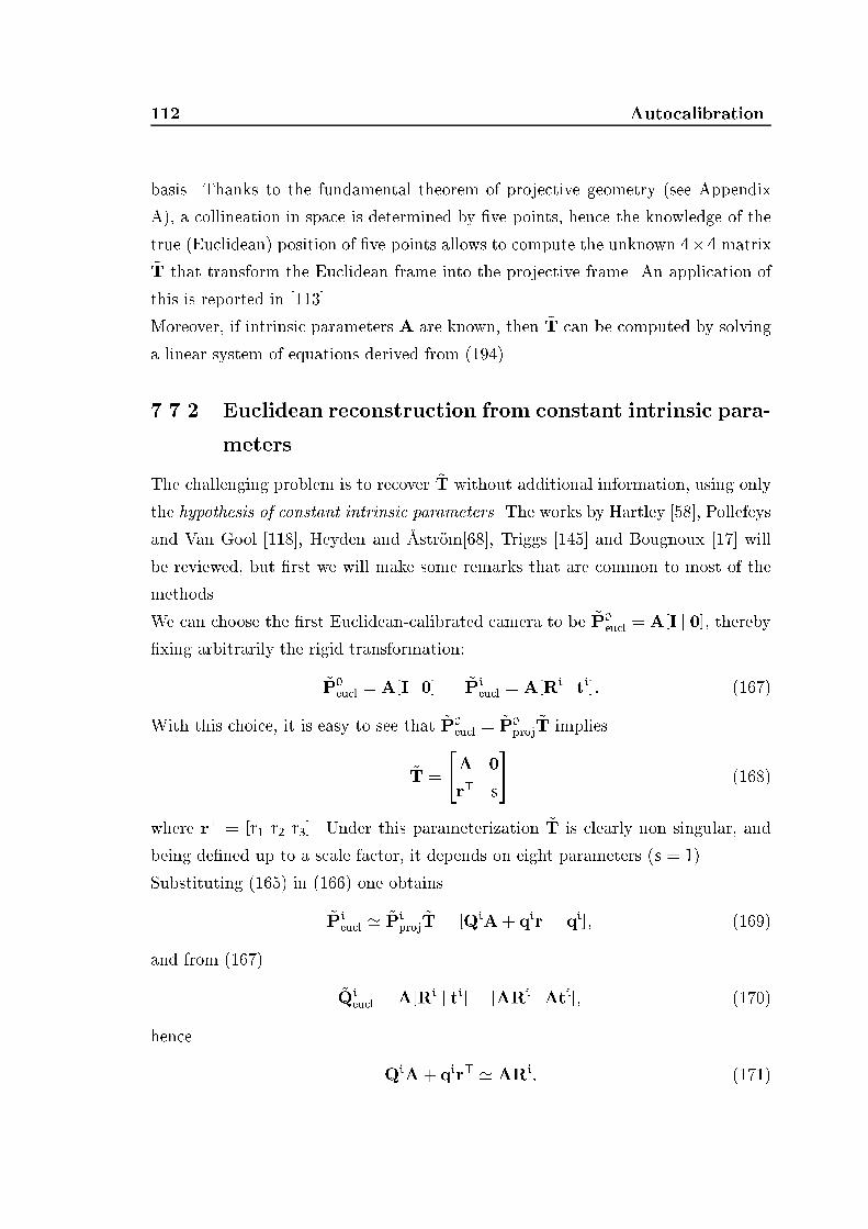
112 Autocalibrationbasis. Thanks to the fundamental theorem of projective geometry (see AppendixA), a collineation in space is determined by �ve points, hence the knowledge of thetrue (Euclidean) position of �ve points allows to compute the unknown 4�4 matrix~T that transform the Euclidean frame into the projective frame. An application ofthis is reported in [113].Moreover, if intrinsic parameters A are known, then ~T can be computed by solvinga linear system of equations derived from (194).7.7.2 Euclidean reconstruction from constant intrinsic para-metersThe challenging problem is to recover ~T without additional information, using onlythe hypothesis of constant intrinsic parameters. The works by Hartley [58], Pollefeysand Van Gool [118], Heyden and �Astr�om[68], Triggs [145] and Bougnoux [17] willbe reviewed, but �rst we will make some remarks that are common to most of themethods.We can choose the �rst Euclidean-calibrated camera to be ~P0eucl = A[I j 0], thereby�xing arbitrarily the rigid transformation:~P0eucl = A[I j 0] ~Pieucl = A[Ri j ti]: (167)With this choice, it is easy to see that ~P0eucl = ~P0proj ~T implies~T = "A 0r> s# (168)where r> = [r1 r2 r3]. Under this parameterization ~T is clearly non singular, andbeing de�ned up to a scale factor, it depends on eight parameters (s = 1).Substituting (165) in (166) one obtains~Pieucl ' ~Piproj ~T = [QiA+ qir> j qi]; (169)and from (167) ~Qieucl = A[Ri j ti] = [ARi j Ati]; (170)hence QiA+ qir> ' ARi: (171)

7.7 Strati�cation 113This is the basic equation, relating the unknowns A (�ve parameters) and r (threeparameters) to the available data Qi and qi. R is unknown, but must be a rotationmatrix.A�ne reconstruction. Equation (171) can be rewritten asQi + qir>A-1 ' ARiA-1 = Hi1; (172)relating the unknown vector a> = r>A-1 to the homography of the in�nity plane(compare (172) with (152)). It can be seen that T factorizes as follows~T = " I 0a> 1#"A 00> 1# : (173)The right-hand matrix is an a�ne transformation, not moving the in�nity plane,whereas the left-hand one is a transformation moving the in�nity plane.Substituting the latter into (166) we obtain:~Pieucl "A-1 00> 1# = ~Pia� ' ~Piproj " I 0a> 1# = [Hi1jqi] (174)Therefore, the knowledge of the homography of the in�nity plane (given by a) allowsto compute the Euclidean structure up to an a�ne transformation, that is an a�nereconstruction.From a�ne to Euclidean. Another useful observation is, if H1 is known andthe intrinsic parameters are constant, the intrinsic parameters matrix A can easilybe computed. In other words, updating from a�ne to Euclidean reconstruction isstraightforward.Let us consider the case of two cameras. If A 0 = A, then H1 is exactly known(with the right scale), sincedet(H1)= det(ARA-1) = 1: (175)From (153) we obtain R = A0-1H1A; and, since RR> = I, it is easy to obtain:H1KH>1 = K (176)

114 Autocalibrationwhere K = AA> is the Kruppa coe�cients matrix. As (176) is an equality between3 � 3 symmetric matrices, we obtain a linear system of six equations in the �veunknown k1; k2; k3; k4; k5 . In fact, only four equations are independent [94, 155],hence at least three views (with constant intrinsic parameters) are required to obtainan over-constrained linear system, which can be easily solved with a linear least-squares technique.Note that two views would be su�cient under the usual assumption that the imagereference frame is orthogonal ( = 0), which gives the additional constraint k3k5 =k2 [94, 155].If points at in�nity (in practice, su�ciently far from the camera) are in the scene,H1can be computed from point correspondences, like any ordinary plane homography[155] Moreover, with additional knowledge, it can be estimated from vanishing pointsor parallelism [37, 34].In the rest of the section, some of the most promising strati�cation techniques willbe reviewed.HartleyHartley [58] pioneered this kind of approach. Starting from (171), we can write(Qi + qia>)A ' ARi: (177)By taking the QR decomposition of the left-hand side we obtain an upper triangularmatrix Bi such that (Qi + qia>)A = BiRi; so (177) rewritesBiRi = �iARi or 1�iA-1Bi = I: (178)The scale factor 1=�i can be chosen so that the sum of the squares of the diagonalentries of (1=�i)A-1Bi equals three. Each camera excluding the �rst, gives sixconstraints in eight unknowns, so three cameras are su�cient. In practice there aremore than three cameras, and the non-linear least squares problem can be solvedwith Levenberg-Marquardt minimization algorithm [48]. As noticed in the case ofKruppa equations, a good initial guess for the unknowns A and a is needed in orderfor the algorithm to converge to the solution.Given that from Hi1 the computation of A is straightforward, a guess for a (thatdetermines Hi1) is su�cient. The cheirality constraint [62] is exploited by Hartley

7.7 Strati�cation 115to estimate the in�nity plane homography, thereby obtaining an approximate a�ne(or quasi-a�ne) reconstruction.Pollefeys and Van GoolIn this approach [118], a projective reconstruction is �rst updated to a�ne recon-struction by the use of the modulus constraint [94, 119]: since the left-hand part of(172) is conjugated to a (scaled) rotation matrix, all eigenvalues must have equalmoduli. Note that this holds if and only if intrinsic parameters are constant. Tomake the constraint explicit we write the characteristic polynomial:det(Qi + qia> - �I) = l3�3 + l2�2 + l1�+ l0: (179)The equality of the roots of the characteristic polynomial is not easy to impose, buta simple necessary condition holds: l3l31 = l32l0: (180)This yields a fourth order polynomial equation in the unknown a for each cameraexcept the �rst, so a �nite number of solutions can be found for four cameras. Somesolutions will be discarded using the modulus constraint, that is more stringent than(180).As discussed previously, autocalibration is achievable with only three views. Itis su�cient to note that, given three cameras, for every plane homography, thefollowing holds [94]: H1;3 = H2;3H1;2: (181)In particular it holds for the in�nity plane homography, soHi;j1 = Hj1Hi1-1 ' (Qj + qja>)(Qi + qia>)-1: (182)In this way we obtain a constraint on the plane at in�nity for each pair of views.Let us write the characteristic polynomial:det((Qj + qja>)(Qi + qia>)-1 - �I) = 0 () (183)det((Qj + qja>) - �(Qi + qia>)) = 0 (184)

116 AutocalibrationWriting the constraint (180) for the three views, a system of three polynomial ofdegree four in three unknowns is obtained. Here, like in the solution of Kruppaequations, homotopy continuation methods could be applied to compute all the43 = 64 solutions.In practice more than three views are available, and we must solve a non-linear least-squares problem: Levenberg-Marquardt minimization is used by the author. Theinitial guess leading to convergence is obtained by starting form a quasi-Euclidean[10] reconstruction, i.e., a reconstruction such that (171) is approximately satis�ed.This can be achieved by approximate knowledge of camera parameters and motionor by using Hartley's method for computing a quasi-a�ne reconstruction.Heyden and �Astr�omThe method proposed by Heyden and �Astr�om [68] is again based on (171), whichcan be rewritten as ~Piproj " Ar> # ' ARi: (185)Since RiRi> = I it follows that:~Piproj " Ar> #" Ar> #> ~Pi>proj = ~Piproj " AA> Arr>A> r>r # ~Pi>proj ' ARiRi>A> = AA>:(186)Note that (186) contains �ve equations, because the matrices of both members aresymmetric, and the homogeneity reduces the number of equations with 1. Hence,each camera matrix, apart from the �rst one, gives �ve equations the eight un-knowns �u; �v; ; u0; v0; r1; r2; r3: A unique solution is obtained when three camerasare available. If the unknown scale factor is introduced explicitly, (186) rewrites:0 = fi(A; r; �i) = �2iAA> - ~Piproj " AA> Arr>A> r>r # ~Pi>proj: (187)Therefore, 3 cameras yield 18 equations in 11 unknowns.

7.7 Strati�cation 117TriggsTriggs [145] proposed a method based on the absolute quadric and, independentlyfrom Heyden and �Astr�om, he derived an equation closely related to (186). Theabsolute quadric consists of planes tangent to the absolute conic [33], and in anEuclidean frame, is represented by the matrixeuc = "I 00 0# : (188)If ~T is a projective transformation acting as in (166), then it can be veri�ed [145]that it transforms euc into = ~Teuc ~T>: Since the projection of the absolutequadric yields the dual image of the absolute conic [145], one obtain~Piproj ~Pi>proj ' K (189)from which, assuming (168), (186) follows immediately. Triggs, however, does notassume any particular form for ~T, hence the unknown are K and. Note that boththese matrix are symmetric and de�ned up to a scale factor.Let k be the matrix composed by the the six elements of the lower triangle of K,and !!! be the matrix composed by the six elements of the lower triangle of , then(186) is equivalent to !!!^ k = 0 (190)in which the unknown scale factor is eliminated. For each camera this amounts to15 bilinear equations in 9 + 5 unknowns, since both k and !!! are de�ned up to ascale factor. Since only �ve of them are linearly independent, at least three imagesare required for a unique solution.Triggs uses two methods for solving the non-linear least-squares problem: sequentialquadratic programming [48] on N � 3 cameras, and a quasi-linear method with SVDfactorization on N � 4 cameras. He recommend to use data standardization (seeSection 5.4.1) and to enforce det() = 3. The sought transformation ~T is computedby taking the eigen-decomposition of .BougnouxThis methods [17] is di�erent from the previous ones, because it does not requireconstant intrinsic parameters and because it achieves an approximate Euclidean

118 Autocalibrationreconstruction without obtaining meaningful camera parameters as a by-product.Let us write (166) in the following form:~Pieucl = 2664 qi>1qi>2 qiqi>3 3775 ' ~Piproj ~T (191)where qi>1 ;qi>2 ;qi>3 are the rows of ~Pieucl: The customary assumptions = 0 and�u = �v, are used to constraint the Euclidean camera matrices: = 0 () (qi1 ^ qi3)>(qi2 ^ qi3) = 0 (192)�u = �v () jjqi1 ^ qi3jj = jjqi2 ^ qi3jj: (193)Thus each camera, excluding the �rst, gives two constraints of degree four. Since wehave six unknown, at least four cameras are required to compute ~T. If the principalpoint (u0; v0) is forced to the image center, the unknowns reduce to four and onlythree cameras are needed.The non-linear minimization required to solve the resulting system is rather unstableand needs to be started in a close initialization: we need to estimate the focal lengthand r. Assuming known principal point, no skew, and unit aspect ratio, the focallength can be computed from the Kruppa equations in closed form [17]. Then,assuming known intrinsic parameters A, an estimation of r can be computed bysolving a linear least-squares problem. From (186) the following is obtained:QiAA>Qi> +QiArqi> + (QiArqi>)> + jjrjj2qiqi> = �2AA>: (194)Since [AA>]3;3 = K3;3 = 1; then � is �xed. After some algebraic manipulation [17]one ends up with four linear equations in Ar. This method works also with varyingintrinsic parameters, although, in practice, only the focal length is allowed to vary,since principal point is forced to the image center and no skew and unit aspect ratioare assumed. The estimation of the camera parameters is inaccurate, neverthelessBougnoux proves that the reconstruction is correct up to an anisotropic homotethy,which he claims to be enough for the reconstructed model to be usable.

7.8 Discussion 1197.8 DiscussionThe applicability of autocalibration techniques in the real world depends on twoissues: sensitivity to noise and solutions bracketing. The challenge is to devisea method that exhibits graceful degradation as noise increases and needs only anapproximate initialization.As for the Kruppa equations, in [92] the authors compare three solving methods: thehomotopy continuation method, Levenberg-Marquardt and the Iterated ExtendedKalman Filter. From the simulations reported, it appears that all the methodsgive comparable results. However, the homotopy continuation method is suitablefor the case of few displacements, as it would be di�cult to use all the constraintsprovided by a long sequence, and its computational cost would be too high. Iterativeapproaches (Levenberg-Marquardt and Iterated Extended Kalman Filter) are wellsuited to the case where more displacements are available. The main limitation ofall these methods is the sensitivity to the noise in the localization of points.The autocalibration methods based on strati�cation that we described have ap-peared only recently, and only preliminary and partial results are available. Trigg'snon-linear algorithm is reported to be accurate, fast and stable and requires onlyapproximate initialization. Both Hartley's and Pollefey's algorithms require a quasi-a�ne reconstruction to start with; the number of unknown in the latter is only three,whereas in the former is eight. Unfortunately, in Pollefey's work the Euclidean recon-struction is evaluated only visually. Also in Heyden and �Astr�om the reconstructionis assessed only visually, and initialization is taken very close to the ground-truth.Bougnoux's algorithm is quite di�erent form the others, since it does not even try toobtain an accurate Euclidean reconstruction. Assessment of reconstruction qualityis deliberately visual.7.9 ConclusionsThis chapter presented a review of recent techniques for Euclidean reconstructionfrom a single moving camera, with unconstrained motion and unknown constantparameters. Such uni�ed, comparative discussion has not yet been presented in theliterature.

120 AutocalibrationEven though formulations may be di�erent, to all the methods reviewed, much ofthe underlying mathematics is common. However, since problems are inherentlynon-linear, proper formulation is very important to avoid di�culties created by thenumerical computation of the solutions.Despite this problem is far from being completely solved, the more general onein which intrinsic parameters are varying is gaining the attention of researchers.In fact, Bougnoux's method already copes with varying parameters. Heyden and�Astr�om [69] proposed a method that works with varying and unknown focal lengthand principal point. Later, they proved [70] that it is su�cient to know any of the �veintrinsic parameters to make Euclidean reconstruction, even if all other parametersare unknown and varying. A similar method that can work with di�erent types ofof constraints has been recently presented in [117].

Chapter 83-D MotionThis chapter address the 3-D motion problem, where the points correspondencesand the rigid displacement between two sets of 3-D points are to be recovered. Oneapplication is to register sets of 3-D measurements obtained with di�erent recon-struction algorithm or depth measuring devices. The existence of missing points inthe two sets makes the problem di�cult. We present RICP, a robust algorithm forregistering and �nding correspondences in sets of 3-D points with signi�cant per-centages of missing data. RICP exploits LMedS robust estimation to withstand thee�ect of outliers. Our extensive experimental comparison of RICP with an existingmethod (ICP) shows RICP's superior robustness and reliability.8.1 IntroductionThis chapter presents a solution to recovering the rigid transformation (rotationand translation) that brings two 3-D point sets into alignment, when the corres-pondences between points are not known and there exist missing data. Given a setof 3-D points on a rigid body in one Cartesian system, and another set of points fromthe same body in a rotated and translated coordinate system, and given the corres-pondences between 3-D points, to estimate the rotation and translation is called the3-D motion problem (also known as absolute orientation problem). To recover thecorrespondences of the points in the two sets is called the correspondence problem.The two problems are intimately connected; [156] gives a nice illustration of theirmathematical symmetry. Least-squares (LS) solutions are well-known for the ideal121

122 3-D Motionmotion problem, in which both sets contain the same number of points a�ected bymoderate sensor noise [80], but fail for the general motion problem, whereby severalpoints, called outliers, have no correspondence in the other set and may lie far frommatched points.3-D motion estimation is an important problem in many aspects of Computer Vision.First, it can be used to register several range views [24, 31, 132], acquired by activeranging systems like laser scanners [146], to recover an accurate, complete surfacemodel of a 3-D object (reverse engineering). Second, 3-D based motion is useful inthose cases where 3-D data can be reconstructed from 2-D images [49, 75, 83, 156],as we described in this thesis. An intriguing scenario is structure reconstructionfrom unregistered video sequences acquired by an uncalibrated camera. Considerseveral, uncalibrated video sequences of the same scene. Usually each sequence spansa continuous range of viewpoints, but the camera jumps discontinuously betweensequences, and there is no information about such movements. Approximate, point-based Euclidean reconstructions can be computed from each sequence; such 3-Ddata could be registered to integrate independent sequences.A popular method for registering 3-D data sets, without a-priori knowledge of cor-respondences, is the iterative closest point algorithm (ICP) introduced by Besl andMcKay [13], and that has been applied in various vision systems using 3-D sensors.The ICP algorithm is an iterative procedure with each iteration consisting of twosteps. In the �rst one, closest neighboring points are put into correspondences, whilekeeping the current object pose �xed. The second step updates the current regis-tration by least-squares minimization of the displacement of matched point pairs.It can be shown that the iteration converges to a minimum of residual error. Sinceconvergence is only local, the initial position is a critical parameter. [14, 19] reportquantitative studies of ICP performance. The most relevant �ndings for our pur-poses are that (i) the initial registration guess a�ects only the speed of convergence(not registration accuracy), as long as it is chosen within the convergence basinof the target minimum; (ii) accurate registration is possible with no outliers, andrequires very accurate measurements and high numbers of points; (iii) acceptableaccuracy (for reverse engineering) can be achieved with 2-300 points.Here we introduce RICP, an algorithm for registering robustly a limited number ofsparse 3-D points (say about 100) corrupted by signi�cant percentages of outliers.

8.2 A brief summary of ICP 123We replaced the LS minimization of ICP with the robust Least Median of Squares(LMedS) regression [126] to withstand the e�ect of outliers.As shown by our experiments, RICP achieves a larger basin of attraction and moreaccurate registrations than ICP. We noticed that RICP still works with dense data,but the advantages over ICP are smaller unless many outliers are present.[99] also reports a robust registration method based on ICP and LMedS. Theirmethod iterates a 3-step sequence of processes: random sampling, estimation of themotion parameters with ICP, and evaluation. The sequence as a whole makes upthe LMedS algorithm. On the contrary, in our approach, LMedS (with randomsampling) is used inside the ICP, where it replaces the LS rotation estimation. Thisenables us to use a dynamic translation estimate based on outlier-free data in theICP iteration.In the following, Section 8.2 summarizes ICP and its main features, Section 8.3presents RICP, Section 8.4 reports our experimental evaluation of RICP, and Section8.5 discusses RICP's contributions and limitations.8.2 A brief summary of ICPThis section summarizes ICP and some features of our ICP implementation. LetP = fpigNp1 and M = fmigNm1 the two sets of 3-D points to align, which we callrespectively data and model. In general, Np 6= Nm. The problem is to compute therotation R and translation t producing the best alignment of P andM:M = RP + t; (195)meaning that R and t are applied to each point in the set P. In general, thisequation will not be satis�ed exactly by all points, hence the equality should beinterpreted in the least square sense.Let us de�ne the closest point in the model to a data point p ascp(p) = arg minm2M km - pk:We can then summarize ICP as follows:1. Compute the subset of CPs: Y = fm 2 M j p 2 P :m = cp(p)g;

124 3-D Motion2. Compute a LS estimate of the motion bringing P onto Y:(R; t) = argminR;t NpXi=1 kyi -Rpi - tk2: (196)where yi 2 Y and pi 2 P.3. Apply the motion to the data points:P RP + t:4. If the stopping criterion (see below) is satis�ed, exit; else go to 1.The algorithm stops as soon as one of the following conditions is satis�ed:� the mean square error (MSE) d = 1=NpPNpi=1 kyi - pik2 is su�ciently small;� the MSE di�erence between two successive iterations is su�ciently small;� the maximum allowed number of iterations has been reached.It has been proven [13] that ICP converges monotonically to a local minimum of theMSE, an index commonly used along with its derivative with respect to the stepindex [13, 14, 132, 166].For step 1, we have implemented CP algorithms based on exhaustive search (ac-ceptable with small point sets) and k-D trees [13, 166].In step 2, motion parameters are computed using a technique involving the SVD,which has been shown to yield the best global accuracy and stability [87]. Since (195)is satis�ed by the centroids of the point sets as well, we can eliminate translationby de�ning the centralized sets:pc;i = pi - �p and yc;i = yi - �ywhere �p = 1=Np NpXi=1 pi �y = 1=Np NpXi=1 cp(pi):Note that we estimate centroids �p (data) and �y (model) at each iteration, using onlythe Np points that are CP for at least one data point, hence a model point increasesits weight in the computation if it is the CP of several data points.

8.3 RICP: a Robust ICP algorithm 125Problem (196) is then equivalent to the following problem:minR NpXi=1 kyc;i -Rpc;ik2; (197)that is minimized when trace(RK) is maximized [80], whereK = NpXi=1 yc;ip>c;i:If the SVD of K is given by K = VDU>, then the optimal rotation matrix thatmaximizes the trace is R = VU>. The optimal translation is then computed ast = �y -R�p.Extensive experimentation with our ICP implementation con�rmed ICP's good per-formance with full overlap (all points in both views) and initial motion guesses veryclose to the solution, and its sensitivity to outliers (e.g., partial overlap) [14, 19].Outliers skew the distribution of the residuals ri = kyi - (Rpi + t)k (Figure 52),and consequently LS motion estimates. In addition, outliers skew the centroid es-timate, and consequently rotation estimates obtained after shifting data points tothe centroid [80].0 0.1 0.2 0.3 0.4

0

5

10

15

20

25

residuals

0 0.5 1 1.50

5

10

15

20

25

30

35

40

residuals

Figure 52: Residual distributions for synthetic point sets corrupted by Gaussiannoise should be Gaussian, but are skewed by outliers. Two realizations of residualsare shown, with full (left) and partial (right) overlap, for one of the last iterations.8.3 RICP: a Robust ICP algorithmThis section outlines RICP, our robust algorithm for correspondenceless point match-ing. Problem and notation are the same as in Section 8.2. RICP replaces step 2

126 3-D Motionof ICP with a robust estimation of motion, based on LMedS. The principle behindLMedS is the following: given a regression problem, where the number of parametersis d, compute a candidate model based on a randomly chosen d-tuple from the data;estimate the �t of this model to all the data, de�ned as the median of the residuals,and repeat optimizing the �t. The data points that do not belong to the optimalmodel, which represent the majority of the data, are outliers. The breakdown point ,i.e., the smallest fraction of outliers that can yield arbitrary estimate values, is 50%.In principle all the d-tuples should be evaluated; in practice a Monte Carlo tech-nique is applied, in which only a random sample of them of size m is considered.Assuming that the whole set of points may contain up to a fraction � of outliers,the probability that at least one of the m d-tuple consist of d inliers is given byP = 1- (1- (1- �)d)m: (198)Hence, given d, �, and the required P (close to 1), one can determine m:m = log(1- P)log(1- (1- �)d) : (199)In our implementation we assume � = 0:5; and require P = 0:95, thus m = 1533:When Gaussian noise is present in addition to outliers, the relative statistical ef-�ciency (i.e., the ratio between the lowest achievable variance for the estimatedparameters and the actual variance) of the LMedS is low; to increase the e�ciency,it is advisable to run a weighted LS �t after LMedS, with weights depending on theresidual of the LMedS procedure [126].Estimating rotation. As in the previous case, we �rst eliminate translation byshifting data and model in the centroid (see next subsection), then, releasing tem-porarily the orthogonality constraint on R, we cast the problem of computing therotation R as a linear regression problem:�yc;1 : : :yc;Np� = R �pc;1 : : :pc;Np�which can be re-written as follows:2664 X 0 00 X 00 0 X 37752664 r1r2r3 3775 = b (200)

8.4 Experimental results 127where X = 2664 p>c;1: : :p>c;Np3775 R = 2664r>1r>2r>3 3775 ;and b is obtained by juxtaposing the rows of the matrix [yc;1 : : :yc;Np]. The nineentries ofR are then computed by solving the linear regression with the Monte CarloLMedS method, outlined before.The residuals sj, j = 1; : : : ; 3Np of (200) are used to generate the weights for the�nal, weighted LS regression as follows. First, a robust standard deviation estimate[126] is computed as � = 1:4826�1+ 52Np - d+ 1�rmedj s2j ; (201)where d is the number of parameters (9 in our case). Second, a weight is assignedto each residual, such thatwj = � 1 if jsjj=� � 2:5;0 otherwise:Notice that the wj are associated to the individual coordinates of 3-D data pointpc;i. A weight w�i is assigned to each point pc;i, which is zero if at least one of itscoordinates has a zero weight, and one otherwise. We therefore deem a point pc;ian outlier if at least one of its coordinates is an outlier. Finally, we estimate R bysolving (197) with each point weighted by w�i . We use SVD to solve the weighted LSproblem (similarly to Section 8.2), which yields a rotation matrix by construction.Estimating centroids. As outliers skew centroid estimates, we adopt a weightedversion of the dynamic average (Section 8.2) taking the average on the outlier-freedata: �p =PNpi=1w�ipi and �m =PNpi=1w�i cp(pi):8.4 Experimental resultsSynthetic data. A �rst set of experiments was devoted to compare the accuracyand robustness of RICP and ICP with controlled noise and outliers. We generatedmodel sets of 50 random points each within a unitary cube (performance depends

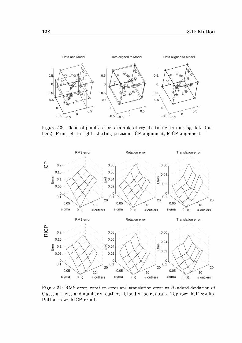
128 3-D Motion

−0.50

0.5

−0.5

0

0.5

−0.5

0

0.5

Data and Model

−0.50

0.5

−0.5

0

0.5

−0.5

0

0.5

Data aligned to Model

−0.50

0.5

−0.5

0

0.5

−0.5

0

0.5

Data aligned to Model

Figure 53: Cloud-of-points tests: example of registration with missing data (out-liers). From left to right: starting position, ICP alignment, RICP alignment.

ICP

0

10

20

0

0.05

0.10

0.05

0.1

0.15

0.2

# outliers

RMS error

sigma

Erm

s

0

10

20

0

0.05

0.10

0.02

0.04

0.06

0.08

# outliers

Rotation error

sigma

Ero

t

0

10

20

0

0.05

0.10

0.02

0.04

0.06

# outliers

Translation error

sigma

Etr

as

RIC

P

0

10

20

0

0.05

0.10

0.05

0.1

0.15

0.2

# outliers

RMS error

sigma

Erm

s

0

10

20

0

0.05

0.10

0.02

0.04

0.06

0.08

# outliers

Rotation error

sigma

Ero

t

0

10

20

0

0.05

0.10

0.02

0.04

0.06

# outliers

Translation error

sigma

Etr

as

Figure 54: RMS error, rotation error and translation error vs standard deviation ofGaussian noise and number of outliers. Cloud-of-points tests. Top row: ICP results.Bottom row: RICP results.

8.4 Experimental results 129on shape [19], but a reasonable indication of performance is achieved with non-elongated sets of random points). The data sets were obtained by translating androtating the models (t = (0:2; 0:1; 0:4)>, rotation by 0.17 rad around axis (1; 1; 1)>;notice the small rotation to guarantee ICP convergence to the correct alignment)and adding Gaussian noise of varying standard deviation. Following [156] outlierswere simulated by dropping points at random from both sets, but avoiding to dropcorresponding pairs from the two sets. For each noise and outlier level, we averagedand recorded the RMS errors, the absolute rotation and translation errors over 50di�erent realizations of noise and outliers.Figure 53 shows a typical example of �nal alignment for ICP and RICP with outliers;the cubes attached to the data emphasize the di�erent quality of the results. Figure54 summarizes the results, suggesting the better accuracy of RICP. The �gure plotsthe RMS, rotation and translation errors against the intensities of Gaussian noise andoutliers (up to 20 points, that 40% of the data). The rotation and translation errorsare the Frobenius norms of the di�erence between the true and estimated R and t,respectively. These measures were chosen because (a) they are simple, scalar indices,(b) errors in the direction of the rotation axis (used previously) were arti�cially highwith small rotations, which make axis estimates poorly conditioned, and (c) the RMSerror (but not both Frobenius norms of R and t) may be small for completely wrongalignments with certain shapes. Notice that, with no outliers, the RMS follows thestandard deviation of the Gaussian noise, as one expects; in this case RICP bene�tsfrom �nal the weighted LS estimation, its performances being the same as ICP.With outliers, the increase of all error indices with the number of outliers is muchsharper for ICP than for RICP. The performance degradation of both algorithmsseems comparable with 40% outliers (recall that the initial displacement is small toensure ICP convergence).We veri�ed the better accuracy of RICP also with di�erent shapes. Figure 55visualizes an example of �nal registration with outliers using as model points thecorners of a standard calibration jig formed by regular grids of squares arrangedon two perpendicular planes. Notice that, unlike the cloud of points above, whichspans 3-D volumes, these data are surfaces. Figure 56 shows the results of the sametype of tests leading to Figure 54.

130 3-D Motion

0 0.5 1 00.5

1−0.8

−0.6

−0.4

−0.2

0

0.2

0.4

Data and Model

0 0.5 1 00.5

1−0.8

−0.6

−0.4

−0.2

0

0.2

0.4

Data aligned to Model

0 0.5 1 00.5

1−0.8

−0.6

−0.4

−0.2

0

0.2

0.4

Data aligned to Model

Figure 55: Calibration jig tests: example of registration with missing data (outliers).From left to right: starting position, ICP alignment, RICP alignment.

ICP

0

10

20

0

0.05

0.10

0.05

0.1

0.15

0.2

# outliers

RMS error

sigma

Erm

s

0

10

20

0

0.05

0.10

0.05

0.1

# outliers

Rotation error

sigma

Ero

t

0

10

20

0

0.05

0.10

0.02

0.04

0.06

0.08

# outliers

Translation error

sigma

Etr

as

RIC

P

0

10

20

0

0.05

0.10

0.05

0.1

0.15

0.2

# outliers

RMS error

sigma

Erm

s

0

10

20

0

0.05

0.10

0.05

0.1

# outliers

Rotation error

sigma

Ero

t

0

10

20

0

0.05

0.10

0.02

0.04

0.06

0.08

# outliers

Translation error

sigma

Etr

as

Figure 56: RMS error, rotation error and translation error vs. standard deviation ofGaussian noise and number of outliers. Calibration jig tests. Top row: ICP results.Bottom row: RICP results.

8.4 Experimental results 131

0 50 100 150 2000

0.05

0.1

0.15

0.2

0.25

0.3

0.35

rotation angle

RM

S e

rror

0 50 100 150 2000

0.5

1

1.5

2

rotation angle

rota

tion

erro

r

Figure 57: Basins of attraction. Final RMS (left) and rotation error (right) for ICP(dashed line and circles) and RICP (solid line and crosses) with increasing initialrotation angle.In a second set of controlled experiments we veri�ed the larger basin of convergence(the region inR; t space guaranteeing convergence to the correct alignment) of RICPwith respect to ICP, by observing the RMS and rotation errors (de�ned as above)for increasingly di�erent initial rotations (from 0 to 180 degrees). We used sets of 30points within the unitary cube, corrupted by outliers and Gaussian noise as before.Translation was �xed, as we found that rotation has the largest in uence on thebasin of convergence (because translation is eliminated by centroids subtraction).Figure 57 shows an example of results (with rotation axis [1; 1; 1]>, 20% outliers,0.02 noise standard deviation), showing clearly that ICP stops converging beforeRICP (here, by about 35 degrees) as the initial rotation di�erence increases. Figure58 visualizes a case in which ICP does not converge and RICP does, at a parity ofinitial displacement and noise/outliers conditions.

−0.50

0.51

−0.5

0

0.5

−0.5

0

0.5

1

Data and Model

−0.50

0.51

−0.5

0

0.5

−0.5

0

0.5

1

Data aligned to Model

−0.50

0.51

−0.5

0

0.5

−0.5

0

0.5

1

Data aligned to Model

Figure 58: A case in which RICP �nds the correct registration and ICP does not.From left to right: starting position, ICP alignment, RICP alignment.

132 3-D MotionA �nal set of experiments proved that RICP leads to more accurate registrationsthan ICP even with dense data with outliers (partial overlap between views). Forinstance, Figure 59 shows two range views of a mechanical widget, acquired by alaser scanner, and the registration found by RICP. Figure 60 shows the histogramsof the absolute residuals for RICP and ICP, clearly smaller for RICP; the MSE is7.21 for ICP and 5.01 for RICP.0

50100

0

50

1000

20

40

60

Model

050

1000

50

1000

20

40

60

Data

050

1000

50

1000

20

40

60

Data aligned to Model

050

100

0

50

100

0

20

40

60

Data aligned to Model

Figure 59: Two range views of a mechanical widget (top row). The registrationfound by RICP, from two viewpoints (bottom row). All views are subsampled fordisplay.0 2 4 6 8 10

0

20

40

60

80

100RICP

residuals0 2 4 6 8

0

10

20

30

40

50

60

70ICP

residualsFigure 60: Residual histograms for the widget experiment.

8.5 Conclusions 1338.5 ConclusionsWe have presented RICP, a robust version of the ICP algorithm for correspondence-less registration of sparse sets of 3-D points corrupted by sensor noise and outliers.RICP is based on the robust, high-e�ciency estimator, LMedS, and implementsa dynamic, weighted scheme for estimating translation using corresponding pointsonly.Unlike ICP, it works on sparse point sets, and tolerates substantial amounts of wrongmeasurements and missing data. With Gaussian noise only, the performances of ICPand RICP are very similar, and both RMS errors converge to the standard deviationof the noise. With outliers, RICP achieves more accurate alignments than ICP(indeed the better the higher the outlier percentage) and converges to the correctregistration from a wider range of initial displacements.Inevitably, RICP's robustness comes at the cost of a higher complexity. In our testson a SPARCServer 10 running Solaris 2.5, RICP took, on average, 88 seconds toregister synthetic clouds of 50 points with noise and outliers, ICP only half a second.This points strongly to o�-line applications for RICP.

Chapter 9ConclusionsThis thesis makes �ve main contributions.The �rst is a simple and compact recti�cation algorithm, developed in Chapter 3.The correct behavior of the algorithm has been demonstrated with both syntheticand real images. Tests showed that reconstruction performed directly from thedisparities of the recti�ed images does not introduces appreciable errors comparedwith reconstructing from the original images.The second major contribution is a new, e�cient algorithm for stereo correspond-ence, SMW, based on a multi-window approach, and taking advantage of left-rightconsistency (Chapter 4). Tests showed the advantages o�ered by SMW. The adapt-ive, multi-window scheme yields robust disparity estimates in the presence of occlu-sions, and clearly outperforms single-window schemes. Left-right consistency provese�ective in eliminating false matches and identifying occluded regions. In addition,disparity is assigned to occluded points heuristically, thereby achieving reasonabledepth maps even in occluded areas. Uncertainty maps are also computed, allowingthe use of SMW as a module within more complex data fusion frameworks. Asfor any area-based matching method, SMW's performance is a�ected adversely bypoorly-textured regions, but areas of low texture are associated consistently withhigh uncertainty values.Another contribution of this thesis is a robust extension of the Shi-Tomasi-Kanadetracker, based on the X84 outlier rejection rule (Chapter 6). The computationalcost is much less than that of schemes based on robust regression and randomsampling like RANSAC or LMedS. Yet experiments indicate excellent reliability135

136 Conclusionsin the presence of non-a�ne feature warping. The algorithm locates and discardsunreliable features accurately and consistently (most right features are preserved,all wrong features are rejected), and tracks good features reliably over many frames.The fourth major contribution is an original, uni�ed account of some of the mostpromising techniques for computing the Euclidean structure from uncalibrated im-ages (Chapter 7). Such a comparative account, which does not yet exist in theliterature, sheds light on the relations between di�erent methods, presented in dif-ferent ways and formalisms in the original research articles.The last contribution of this thesis is RICP, a robust version of the ICP algorithmfor correspondenceless registration of sparse sets of 3-D points corrupted by sensornoise and outliers (Chapter 8). RICP is based on LMedS regression, and implementsa dynamic, weighted scheme for estimating translation using corresponding pointsonly. Unlike ICP, it works on sparse point sets, and tolerates substantial amountsof wrong measurements and missing data. Inevitably, RICP's robustness comes atthe cost of a higher complexity, and this points strongly to o�-line applications forRICP.These �ve contributions cover the main elements for building a robust system forstructure recovery, coping with various degrees of a-priori knowledge. A completesystem should include projective reconstruction and autocalibration, that could notbe implemented during this research.

Appendix AProjective GeometryMine eye hath play'd the painter, and hath stell'dThy beauty's form in table of my heart;My body is the frame wherein 'tis held,And perspective it is best painter's art.For through the painter must you see his skill,To �nd where your true image pictur'd lies,...1The understanding of perspective projections was one of the great achievements ofthe Rinascimento (Reneissance). The Italian architect F. Brunelleschi studied thistopic in some detail, but the �rst explicit formulation of perspective projections isfound in the treatise by L. B. Alberti De Pictura [1], written in 1435. This treatisedescribes a method for projecting the horizontal \plane of the oor" onto the vertical\plane of the painting". Piero della Francesca pushed the theory forward: in hisDe Prospectiva Pingendi [29], written in 1478, he dealt with the general problem ofdepicting 3-D objects and, as a painter, he also put his theory in practice (Figure62).In the XVII century G. Desargues, building on the works on perspective and on astro-nomical research by Keplero, introduced projective geometry as a tool for studyingthe conics (see [135]). Projective geometry, thanks to the concept of points at in-�nity, deals with elegance with all the particular cases found in theorems on conics.1W. Shakespeare, Complete Sonnets, Dover Publications Inc, NY, 1991137

138 Projective GeometryFrom the analytic standpoint, the most important aspect of projective geometry isthe introduction of homogeneous coordinates, which allows many of the signi�cantaspects of projective geometry to be proven using linear algebra.In this appendix some concepts of analytic projective geometry will be brie y re-viewed and summarized for the reader's convenience. A more detailed knowledge ofthe subject can be acquired by reading [6, 160, 107, 33].

Figure 61: The well-known \Flagellazione" byPiero della Francesca, painted in 1460, GalleriaNazionale delle Marche, Urbino. This paintinghave been studied as one of the most importantexamples of perspective drawing [159]. Figure 62: \La camera degliSposi" by Andrea Mantegnapainted in fresco in 1474,Palazzo Ducale, Mantova.Points and lines A point on the projective plane is represented by an orderedtriple of real numbers [x1; x2; x3] 6= [0; 0; 0] with the convention that [x1; x2; x3] and[�x1; �x2; �x3] { where � 6= 0 { represent the same point.A line on the projective plane is represented by an ordered triple of real numbers[x1; x2; x3] 6= [0; 0; 0] with the convention that [x1; x2; x3] and [�x1; �x2; �x3] where� 6= 0 represents the the same line . We shall see that a suitable coordinate systemcan be established in the plane, so that this number triplets are the coordinates ofpoints.Projective basis Four points a1; a2; a3; a4, no three of which are collinear, de�nea projective basis for the projective plane. Let us choose the representations (i.e., the

139scale factors) of the �rst three points so that we have: a1+a2+a3 = a4. In terms ofthis coordinate system, we de�ne the relative homogeneous coordinates of any pointsx to be [x1; x2; x3] if x = x1a1 + x2a2 + x3a3. The word \homogeneous" refers tothe fact that the homogeneous coordinates of a projective point may be multipliedby any nonzero scalar. Note that the role of a4 is simply to �x the scale factors fora1; a2 and a3, which can be otherwise chosen arbitrarily. Indeed, if x = [x1; x2; x3]and we change the representation for the reference points, the linear combinationx1�1a1 + x2�2a2 + x3�3a3 gives a representation of a point di�erent from x.Any point [x1; x2; x3] may be written as x1[1; 0; 0] + x2[0; 1; 0] + x3[0; 0; 1]; hence, re-ferred to this coordinate system, it has relative homogeneous coordinates [x1; x2; x3].The coordinate system de�ned by the four points [1; 0; 0]; [0; 1; 0]; [0; 0; 1]; [1; 1; 1] iscalled the natural coordinate system.Collinear points In the projective plane, points and lines are dual elements; thepoint x belongs to the line y if an only if their scalar product is zero, in symbolsx � y = 0: (202)When x is a variable point on the �xed line y, (202) is called the equation of theline.It can be easily proved that a necessary and su�cient condition for the distinctpoints x, y, z to be collinear is det(x;y; z) = 0; (203)which is equivalent to x � (y^ z) = 0: (204)Hence the line containing the two distinct points y e z is represented by (y ^ z).It can also be proved that if y e z are distinct points, then �y+�z with �; � 2 R+is another point on the line determined by y e z. If we let � = �=� and accept theconvention y + �z = z when � = 1, the line containing the two distinct points yand z has parametric equation:x = y + �z � 2 R [ f1g : (205)

140 Projective GeometryCollineations A non-singular linear transformation of the projective plane intoitself is called collineation (or homography).The most general collineation is represented by a non-singular 3� 3 matrix H:2664 �x 01�x 02� 3775 = 2664H1;1 H1;2 H1;3H2;1 H2;2 H2;3H3;1 H3;2 1 37752664 x1x21 3775 : (206)The collineationmaps points into points and lines into lines and preserves collinearity(hence its name).The projective transformation matrix H requires eight independent parameters tode�ne a unique mapping. Each point correspondence in the plane provides twoequations:24 x1 x2 1 0 0 0 -x1x 01 -x2x 010 0 0 x1 x2 1 -x1x 02 -x2x 02 35

26666666666666664H1;1H1;2H1;3H2;1H2;2H2;3H3;1H3;2

37777777777777775 = " x 01x 02 # : (207)It is then necessary to �nd four point correspondences to de�ne the transformationmatrix uniquely. This gives a constructive proof that four points (provided that nothree of them are collinear) determine a unique transformation matrix. This is inagreement with the fact that a base for the projective plane is composed by fourelements: the collineation is completely speci�ed by its action on a base. This result,generalized in a projective space of any dimension, is known as the fundamentaltheorem of the projective geometry.Cross ratio On the line determined by y and z take four points a = y + �z;b = y + �z; c = y + z and d = y + �z: We de�ne the cross ratio of these pointsin terms of the parameters �; �; ; � as(�; �; ; �) = (�- )(�- �)(�- �)(�- ) : (208)

141The signi�cance of the cross ratio is that it is invariant under collineations. Theparameters �; �; ; � can also be interpreted as the distances from a �xed point onthe line.Models for the projective plane In this paragraph we present two commonmodels of projective spaces.In the �rst model, we build up an a�ne space to form a projective space by insertingthe directions of lines as additional points. The projective plane is built up from thea�ne plane by adding points at in�nity (ideal points) in such a way that parallellines always meet at an ideal point. Hence, we add one ideal point for each pencilof parallel lines. The set of all ideal points form the line at in�nity.In the second method we collapse a vector space to form a projective space byusing the lines in that vector space as our projective points. Let V be an n-dimensional vector space. The associated (n - 1)-dimensional projective space is�V = fQjQ is a 1-dimensional subspace of Vg. A model for the projective plane isconstituted by a pencil of lines in 3-D space, all emanating from the origin, and anarbitrary plane �, not passing through the origin. Each line represents a projectivepoint. The lines which intersect the plane correspond to points in the a�ne plane,whereas lines parallel to � correspond to ideal points. Only the direction of lines isimportant in this model. This is in agreement with the homogeneous representationof projective points.Although both these models are useful to understand projective geometry, the \col-lapsed vector space" approach is less cumbersome since one does not have to discusstwo cases, one for ideal points and the other for a�ne points.Axioms for the projective plane In de�ning the projective plane we took theanalytic approach, introducing immediately coordinates. Yet, projective geometryis often formalized from a synthetic point of view. The following three statementsare usually taken as axioms de�ning the projective plane:(1) Two points are contained in one and only one line.(2) Two lines intersect in exactly one point.(3) There are four points such that no three are on the same line.

142 Projective GeometryHomogeneous vs Cartesian coordinates Homogeneous coordinates (triplets ofreal numbers) are used to represent points on the projective planes. Representationis not unique, since x and �x with � 2 R represent the same projective point.Cartesian coordinates (pairs of real numbers) are used to represent points in thea�ne plane. The representation is unique. Since the projective plane can be viewedas an extended a�ne plane, we can draw a relationship between representationsof a�ne points (ideal points, of course, do not have a Cartesian representation).From the \collapsed vector space" point of view, the Cartesian representation of aprojective point are the coordinates, in the plane � : x3 = 1, of the intersection of theline representing the projective point with the plane �. The Cartesian coordinatescorresponding to a projective point [x1; x2; x3] are [x1=x3; x2=x3]. Vice versa, thehomogeneous representation of the point [x1; x2] is �[x1; x2; 1] with � 2 R+ .

List of symbolsI(�; �) image brightness~P = [Qj~q] perspective projection matrix (camera matrix)~w homogeneous coordinates of a world point~m homogeneous coordinates (in pixels) of an image point~p normalized homogeneous coordinates of an image point (ray vector)� relative depth' equality up to an arbitrary scale factor� arbitrary scale factorF focal planeR retinal plane(u; v) image reference frame(x; y; z) world reference frame(X;Y;Z) camera std reference frameA intrinsic parameters matrixf focal distanceku e�ective pixel horizontal sizekv e�ective pixel vertical size�u focal distance in horizontal pixels�v focal distance in veritcal pixels(u0; v0) principal point skew factorG = [Rjt] extrinsic parameters matrixR rotation matrixt translation vector 143

144 List of Symbolsc optical center^ external product[ ]^ external product matrixdiag(: : : ) diagonal matrix; the arguments are the diagonal elementstrace(�) sum of the diagonal elements of a matrixe epipoleE essential matrixF fundamental matrix[ ]i projection operator extracting the i-th componentH� homography matrix of plane �H1 in�nity plane homography matrixK = AA> Kruppa's coe�cients matrix

CreditsThe software for this thesis was written by the author, with the exceptions listedbelow. It was coded in MATLAB ( c Copyright The Math Works Inc.), SCILAB2,a public domain MATLAB-like package from INRIA (registered at APP under thenumber 93-27-011-00) or in ANSI C, and compiled using the public domain GNUgcc compiler v2.7 ( c Copyright Free Software Foundation, Inc.). Some programsin C inclues Meschach ( c Copyright David E. Stewart), a public domain library forlinear algebra (available from Netlib3) and the Numerical Recipes [120] routines in C( c Copyright Numerical Recipes Software). Images are read, written and visualizedusing the HIPS ( c Copyright SharpImage Software) package. The calibration codeis by Luc Robert4 (INRIA), and the Calibtool interface was written in Tcl/Tk by aErman Petrei (University of Udine). The tracking algorithm was coded by TizianoTommasini [140], and the RICP code is due to Stefano Morson, Orazio Stangherlinand Gerard Martin [98], who also helped in performing the experiments.Computing and laboratory facilities were provided by the Dipartimento di Matem-atica ed Informatica, University of Udine, by courtesy of Vito Roberto. Visits tothe Heriot-Watt University, Edinburgh, was supported by a British Council grantthe �rst time and by a EC Socrates grant the second time.Stereo pairs in Chapter 3 ( c Copyright INRIA-Syntim5) were calibrated by Jean-Philippe Tarel [134]. The stereo pairs \Parking meter", \Shrub", and \Trees" inChapter 4 are part of the JISCT (JPL-INRIA-SRI-CMU-TELEOS) stereo test set6;2http://www-rocq.inria.fr/scilab/scilab.html3http://www.netlib.org/4http://www.inria.fr/robotvis/personnel/lucr/detecproj.html5http://www-syntim.inria.fr/syntim/analyse/paires-eng.html6ftp://ftp.vislist.com/IMAGERY/JISCT/ 145

146 Creditsthe \Castle" stereo pair, with calibration data, is courtesy of Carnegie Mellon Uni-versity | Calibrated Imaging Laboratory7 (supported by ARPA, NSF, and NASA).The \Hotel" and \Artichoke" sequences in chapter 6 are taken from the CarnegieMellon University { VASC8 database. \Platform" is part of the SOFA9 syntheticsequences, courtesy of the Computer Vision Group, Heriot-Watt University. \Stair"is courtesy of Francesco Isgr�o, Heriot-Watt University. Thanks to Bob Fisher andAnthony Ashbrooks (Department of Arti�cial Intelligence, University of Edinburgh)for the widget data used in Chapter 8. The calibration jig was designed by Aless-andro Verri and manufactured at the University of Genova, Department of Phisics.Parts of this dissertation are adapted from papers written by the candidate duringthis three years, in conjuction with other authors: Vito Roberto, Tiziano Tommasini,Emanuele Trucco and Alessandro Verri. In particular, Chapter 3 incorporates arevised version of [46, 42]; Chapter 4 comes from the merging of [44, 45, 124];Chapter 6 is a revised version of [141]; Chapter 7 is based on [43] and Chapter 8 isadapted from [147].

7http://www.cs.cmu.edu/afs/cs/project/cil/www/cil-ster.html8http://www.ius.cs.cmu.edu/idb/9http://www.cee.hw.ac.uk/~mtc/sofa

Bibliography[1] Alberti, L. De pictura. Bari, Italy, 1980. edited by C. Grayson.[2] Anandan, P. A computational framework and an algorithm for the measure-ment of visual motion. International Journal of Computer Vision 2 (1989),283{310.[3] Armstong, M., Zisserman, A., and Hartley, R. Self-calibration fromimage triplets. In Proceedings of the European Conference on Computer Vision(Cambridge, UK, 1996), pp. 5{16.[4] Avidan, S., and Shashua, A. Threading fundamental matrices. In Proceed-ings of the European Conference on Computer Vision (University of Freiburg,Germany, 1998), pp. 124{140.[5] Ayache, N. Arti�cial Vision for Mobile Robots: Stereo Vision and Multis-ensory Perception. The MIT Press, 1991.[6] Ayres, F. Theory and Problems of Projective Geometry. Schaum's OutlineSeries in Mathematics. McGraw-Hill, 1967.[7] Baker, H., and Binford, T. Depth from edge and intensity based stereo.In Proceedings of the International Joint Conference on Arti�cial Intelligence(1981), pp. 631{636.[8] Barnard, S. T., and Thompson, W. B. Disparity analysis of images.IEEE Transactions on Pattern Analysis and Machine Intelligence 2, 4 (1980),333{340.[9] Barron, J. L., Fleet, D. J., and Beauchemin, S. Performance of optical ow techniques. International Journal of Computer Vision 12, 1 (1994), 43{77.147

148 Bibliography[10] Beardsley, P., Zisserman, A., and Murray, D. Sequential update ofprojective and a�ne structure from motion. International Journal of Com-puter Vision 23, 3 (1997), 235{259.[11] Belhumeur, P. N. A Bayesian approach to binocular stereopsis. Interna-tional Journal of Computer Vision 19, 3 (1996), 237{260.[12] Benedetti, A., and Perona, P. Real-time 2-d feature detection on arecon�gurable computer. In Proceedings of the IEEE Conference on Com-puter Vision and Pattern Recognition (Santa Barbara, CA, June 1998), IEEEComputer Society Press, pp. 586{593.[13] Besl, P., and McKay, N. A method for registration of 3-D shapes. IEEETransactions on Pattern Analysis and Machine Intelligence 14, 2 (February1992), 239{256.[14] Bispo, E. M., and Fisher, R. B. Free-form surface matching for surfaceinspection. In The Mathematics of Surfaces VI, G. Mullineux, Ed. ClarendonPress, Oxford, 1996, pp. 119{136.[15] Blake, R., and Wilson, H. R. Neural models of stereoscopic vision. Trendsin Neuroscience 14 (1991), 445{452.[16] Bolles, R. C., Baker, H. H., and Hannah, M. J. The JISCT stereoevaluation. In Proceedings of the Image Understanding Workshop (Washing-ton, DC, April 1993), ARPA, Morgan Kaufmann, pp. 263{274.[17] Bougnoux, S. From projective to Euclidean space under any practical situ-ation, a criticism of self-calibration. In Proceedings of the IEEE InternationalConference on Computer Vision (Bombay, 1998), pp. 790{796.[18] Brandt, J. W. Improved accuracy in gradient-based optical ow estimation.International Journal of Computer Vision 25, 1 (1997), 5{22.[19] Brujic, D., and Ristic, M. Analysis of free-form surface registration.In Proceedings of the IEEE International Conference on Image Processing(Lausanne, Switzerland, 1996), vol. II, pp. 393{396.

Bibliography 149[20] Campani, M., and Verri, A. Motion analysis from �rst order propertiesof optical ow. CVGIP: Image Understanding 56 (1992), 90{107.[21] Campus, O., Flynn, P. J., and Stockman, G. C., Eds. Special Issueon CAD-Based Computer Vision (March 1998), vol. 69:3 of Computer Visionand Image Understanding.[22] Caprile, B., and Torre, V. Using vanishing points for camera calibration.International Journal of Computer Vision 4 (1990), 127{140.[23] Charnley, D., and Blisset, R. J. Surface reconstruction from outdoorimage sequences. Image and Vision Computing 7, 1 (1989), 10{16.[24] Chen, Y., and Medioni, G. Object modeling by registration of multiplerange images. Image and Vision Computing 10, 3 (1992), 145{155.[25] Cox, I., Roy, S., and Hingorani, S. Dynamic histogram warping of imagepairs for constant image brightness. In Proceedings of the IEEE InternationalConference on Image Processing (Washington, D.C, 1995), vol. 2, pp. 366{369.[26] Cox, I. J., Hingorani, S., Maggs, B. M., and Rao, S. B. A maximumlikelihood stereo algorithm. Computer Vision and Image Understanding 63, 3(May 1996), 542{567.[27] Dacol, L. Integrazione di tecniche per la ricostruzione di forme in visionearti�ciale. Tesi di laurea in scienze dell'informazione, Universit�a degli Studidi Udine, 1998.[28] Davies, E. Machine Vision: Theory, Algorithms, Practicalities, 2nd ed. Aca-demic Press, 1997.[29] della Francesca, P. De Prospectiva Pingendi. Edizione critica. Sansoni,Firenze, Italy, 1942.[30] Dhond, U. R., and Aggarwal, J. K. Structure from stereo { a re-view. IEEE Transactions on Systems, Man and Cybernetics 19, 6 (Novem-ber/December 1989), 1489{1510.

150 Bibliography[31] Eggert, D. W., Fitzgibbon, A. W., and Fisher, R. B. Simultaneousregistration of multiple range views for use in reverse engineering. In Proceed-ings of the International Conference on Pattern Recognition (Vienna, 1996),pp. 243{247.[32] Faugeras, O. What can be seen in three dimensions with an uncalibratedstereo rig? In Proceedings of the European Conference on Computer Vision(Santa Margherita L., 1992), pp. 563{578.[33] Faugeras, O. Three-Dimensional Computer Vision: A Geometric View-point. The MIT Press, Cambridge,MA, 1993.[34] Faugeras, O. Strati�cation of 3-D vision: projective, a�ne, and metricrepresentations. Journal of the Optical Society of America A 12, 3 (1994),465{484.[35] Faugeras, O., Hotz, B., Mathieu, H., Vi�eville, T., Zhang, Z., Fua,P., Th�eron, E., Moll, L., Berry, G., Vuillemin, J., Bertin, P., andProy, C. Real-time correlation-based stereo: algorithm, implementation andapplications. Tech. Rep. 2013, Unit�e de recherche INRIA Sophia-Antipolis,August 1993.[36] Faugeras, O., and Maybank, S. Motion from point matches: multiplicityof solutions. International Journal of Computer Vision 4, 3 (June 1990), 225{246.[37] Faugeras, O., Robert, L., Laveau, S., Csurka, G., Zeller, C.,Gauclin, C., and Zoghlami, I. 3-d reconstruction of urban scenes fromimage sequences. Computer Vision and Image Understanding 69, 3 (March1998), 292{309.[38] Faugeras, O., and Toscani, G. Camera calibration for 3D computervision. In Proceedings of the International Workshop on Machine Vision andMachine Intelligence (Tokyo, Japan, February 1987).[39] Fischler, M. A., and Bolles, R. C. Random Sample Consensus: aparadigm model �tting with applications to image analysis and automatedcartography. Communications of the ACM 24, 6 (June 1981), 381{395.

Bibliography 151[40] Foley, J. D., van Dam, A., Feiner, S. K., Huges, J. F., and Phillips,R. L. Introduction to Computer Graphics. Addison-Wesley, 1990.[41] Fua, P. Combining stereo and monocular information to compute densedepth maps that preserve depth discontinuities. In Proceedings of the Interna-tional Joint Conference on Arti�cial Intelligence (Sydney, Australia, August1991), pp. 1292{1298.[42] Fusiello, A. Tutorial on recti�cation of stereo images. In CVonline: On-Line Compendium of ComputerVision [Online], R. Fisher, Ed. 1998. Available:http://www.dai.ed.ac.uk/CVonline/.[43] Fusiello, A. Uncalibrated Euclidean reconstruction: A review. ResearchReport UDMI/10/98/RR, Dipartimento di Matematica e Informatica, Uni-versit�a di Udine, July 1998. Submitted for publication in Computing.[44] Fusiello, A., Roberto, V., and Trucco, E. E�cient stereo with mul-tiple windowing. In Proceedings of the IEEE Conference on Computer Visionand Pattern Recognition (Puerto Rico, June 1997), IEEE Computer SocietyPress, pp. 858{863.[45] Fusiello, A., Roberto, V., and Trucco, E. Experiments with a newarea-based stereo algorithm. In Proceedings of the 9th International Confer-ence on Image Analysis and Processing (Florence, Italy, September 1997),A. Del Bimbo, Ed., IAPR, Springer, pp. 669{676. Lecture Notes in ComputerScience 1310.[46] Fusiello, A., Trucco, E., and Verri, A. Recti�cation with uncon-strained stereo geometry. In Proceedings of the British Machine Vision Con-ference (September 1997), A. F. Clark, Ed., BMVA Press, pp. 400{409.[47] Geiger, D., Ladendorf, B., and Yuille, A. Occlusions and binocularstereo. International Journal of Computer Vision 14, 3 (April 1995), 211{226.[48] Gill, P., Murray, W., and Wright, M. Practical Optimization. Aca-demic Press, 1981.

152 Bibliography[49] Goldgof, D. B., Lee, H., and Huang, T. Matching and motion estim-ation of three-dimensional point and line sets using eigenstructure withoutcorrespondence. Pattern Recognition 25, 3 (1992), 271{286.[50] Golub, G. H., and Loan, C. F. V. Matrix Computations, third ed. TheJohn Hopkins University Press, 1996.[51] Grimson, W. A computer implementation of a theory of human stereo vis-ion. Philosophical Transactions of the Royal Society of London, B. 292, 1058(1981), 217{253.[52] Grimson, W. Computational experiments with a feature based stereo al-gorithm. IEEE Transactions on Pattern Analysis and Machine Intelligence 7,1 (January 1985), 17{34.[53] Grimson, W. E. L. From Images to Surfaces. The MIT Press, 1981.[54] Hager, G., and Belhumeur, P. Real-time tracking of image regions withchanges in geometry and illumination. In Proceedings of the IEEE Confer-ence on Computer Vision and Pattern Recognition (San Francisco, CA, 1996),pp. 403{410.[55] Hampel, F., Rousseeuw, P., Ronchetti, E., and Stahel, W. Ro-bust Statistics: the Approach Based on In uence Functions. Wiley Series inprobability and mathematical statistics. John Wiley & Sons, 1986.[56] Hannah, M. A system for digital stereo image matching. PhotogrammaticEngineering and Remote Sensing (1989), 1765{1770.[57] Harris, C., and Stephens, M. A combined corner and edge detector.Proceedings of the 4th Alvey Vision Conference (August 1988), 189{192.[58] Hartley, R. Euclidean reconstruction from uncalibrated views. In Applica-tions of Invariance in Computer Vision (1993), J. Mundy and A. Zisserman,Eds., vol. 825 of Lecture Notes in Computer Science, Springer-Verlag, pp. 237{256.

Bibliography 153[59] Hartley, R. Self-calibration from multiple views with a rotating camera.In Proceedings of the European Conference on Computer Vision (Stockholm,1994), pp. 471{478.[60] Hartley, R., and Gupta, R. Computing matched-epipolar projections. InProceedings of the IEEE Conference on Computer Vision and Pattern Recog-nition (1993), pp. 549{555.[61] Hartley, R. I. Estimation of relative camera position for uncalibrated cam-eras. In Proceedings of the European Conference on Computer Vision (SantaMargherita L., 1992), pp. 579{587.[62] Hartley, R. I. Cheirality invariants. In Proceedings of the Image Under-standing Workshop (Washington, DC, April 1993), ARPA, Morgan Kaufmann,pp. 745{753.[63] Hartley, R. I. In defence of the 8-point algorithm. In Proceedings of theIEEE International Conference on Computer Vision (1995).[64] Hartley, R. I. Kruppa's equations derived from the fundamental matrix.IEEE Transactions on Pattern Analysis and Machine Intelligence 19, 2 (Feb-ruary 1997), 133{135.[65] Hartley, R. I. Minimizing algebraic error. In Proceedings of the IEEEInternational Conference on Computer Vision (Bombay, 1998).[66] Hartley, R. I., and Sturm, P. Triangulation. Computer Vision andImage Understanding 68, 2 (November 1997), 146{157.[67] Henkel, R. D. Fast stereovision with subpixel-precision. In Proceedingsof the IEEE International Conference on Computer Vision (Bombay, 1998),pp. 1024{1028.[68] Heyden, A., and �Astr�om, K. Euclidean reconstruction from constant in-trinsic parameters. In Proceedings of the International Conference on PatternRecognition (Vienna, 1996), pp. 339{343.

154 Bibliography[69] Heyden, A., and �Astr�om, K. Euclidean reconstruction from image se-quences with varying and unknown focal length and principal point. In Pro-ceedings of the IEEE Conference on Computer Vision and Pattern Recognition(Puerto Rico, 1997), pp. 438{443.[70] Heyden, A., and �Astr�om, K. Minimal conditions on intrinsic paramet-ers for Euclidean reconstruction. In Proceedings of the Asian Conference onComputer Vision (Hong Kong, 1998).[71] Horn, B. Relative orientation. International Journal of Computer Vision 4,1 (January 1990), 59{78.[72] Horn, B. Relative orientation revisited. Journal of the Optical Society ofAmerica A 8, 10 (October 1991), 1630{1638.[73] Huang, T. S., and Netravali, A. N. Motion and structure from featurecorrespondences: A review. Proceedings of IEEE 82, 2 (1994), 252{267.[74] Intille, S. S., and Bobick, A. F. Disparity-space images and large occlu-sion stereo. In European Conference on Computer Vision (Stockholm, Sweden,May 1994), J.-O. Eklundh, Ed., Springer-Verlag, pp. 179{186.[75] Ito, E., and Aloimonos, Y. Is correspondence necessary for the percep-tion of structure from motion? In Proceedings of the Image UnderstandingWorkshop (1988), pp. 921{929.[76] Jenkin, M. R. M., and Jepson, A. D. Recovering local surface structurethrough local phase di�erence measurements. CVGIP: Image Understanding59, 1 (1994), 72{93.[77] Jenkin, M. R. M., Jepson, A. D., and Tsotsos, J. K. Techniques fordisparity measurements. CVGIP: Image Understanding 53, 1 (1991), 14{30.[78] Jones, D. G., and Malik, J. Computational framework for determiningstereo correspondence from a set of linear spatial �lters. Image and VisionComputing 10, 10 (1992), 699{708.

Bibliography 155[79] Kanade, T., and Okutomi, M. A stereo matching algorithm with anadaptive window: Theory and experiments. IEEE Transactions on PatternAnalysis and Machine Intelligence 16, 9 (September 1994), 920{932.[80] Kanatani, K. Geometric Computation for Machine Vision. Oxford Univer-sity Press, 1993.[81] Kass, M., Witkin, A., and Terzopulos, D. Snakes: Active contourmodels. International Journal of Computer Vision 1, 4 (1988), 321{331.[82] Kruppa, E. Zur Ermittlung eines Objektes aus zwei Perspektiven mit innererOrientierung. Sitz.-Ber. Akad. Wiss., Wien, math. naturw. Kl., Abt. IIa. 122(1913), 1939{1948.[83] Lee, C., and Joshi, A. Correspondence problem in image sequence analysis.Pattern Recognition 26 (1993), 47{61.[84] Lindeberg, T. Scale space for discrete signals. IEEE Transactions on Pat-tern Analysis and Machine Intelligence 12 (1990), 234{254.[85] Little, J. J., and Gillett, W. E. Direct evidence for occlusions in stereoand motion. Image and Vision Computing 8, 4 (November 1990), 328{340.[86] Longuet-Higgins, H. C. A computer algorithm for reconstructing a scenefrom two projections. Nature 293, 10 (September 1981), 133{135.[87] Lorusso, A., Eggert, D. W., and Fisher, R. B. A comparison offour algorithms for estimating 3-D rigid transformations. Machine Vision andApplications 9 (1997), 272{290.[88] Lowe, D. Fitting parameterized three-dimensional models to images. IEEETransactions on Pattern Analysis and Machine Intelligence 13, 5 (May 1991),441{450.[89] Lucas, B. D., and Kanade, T. An iterative image registration techniquewith an application to stereo vision. In Proceedings of the International JointConference on Arti�cial Intelligence (1981).

156 Bibliography[90] Ludwig, K. O., Neumann, H., and Neumann, B. Local stereoscopicdepth estimation. Image and Vision Computing 12, 10 (1994), 16{35.[91] Luong, Q.-T., Deriche, R., Faugeras, O., and Papadopoulo, T.On determining the fundamental matrix: Analysis of di�erent methods andexperimental results. Tech. Rep. 1894, Unit�e de recherche INRIA Sophia-Antipolis, April 1993.[92] Luong, Q.-T., and Faugeras, O. Self-calibration of a moving camerafrom point correspondences and fundamental matrices. International Journalof Computer Vision 22, 3 (1997), 261{289.[93] Luong, Q.-T., and Faugeras, O. D. The fundamental matrix: Theory,algorithms, and stability analysis. International Journal of Computer Vision17 (1996), 43{75.[94] Luong, Q.-T., and Vi�eville, T. Canonical representations for the geomet-ries of multiple projective views. Computer Vision and Image Understanding64, 2 (1996), 193{229.[95] Ma, Y., Ko�seck�a, J., and Sastry, S. Motion recovery from image se-quences: Discrete viewpoint vs. di�erential viewpoint. In Proceedings of theIEEE International Conference on Computer Vision (Bombay, 1998), pp. 337{353.[96] Marr, D., and Poggio, T. Cooperative computation of stereo disparity.Science 194 (1976), 283{287.[97] Marr, D., and Poggio, T. A theory of human stereo vision. A.I. Memo451, Massachusetts Institute of Technology, November 1977.[98] Martin, G. Registrazione di forme in visione arti�ciale. Tesi di laurea inscienze dell'informazione, Universit�a degli Studi di Udine, 1998.[99] Masuda, T., and Yokoya, N. A robust method for registration and seg-mentation of multiple range images. Computer Vision and Image Understand-ing 61, 3 (May 1995), 295{307.

Bibliography 157[100] Maybank, S. J., and Faugeras, O. A theory of self-calibration of a movingcamera. International Journal of Computer Vision 8, 2 (1992), 123{151.[101] Maybeck, P. S. Stochastic Models, Estimation and Control, vol. 1. AcademicPress: New York, NY, 1979.[102] Medioni, G., and Nevatia, R. Segment-based stereo matching. ComputerVision, Graphics, and Image Processing 31, 1 (July 1985), 2{18.[103] Meer, P., Mintz, D., Kim, D. Y., and Rosenfeld, A. Robust regressionmethods in computer vision: a review. International Journal of ComputerVision 6 (1991), 59{70.[104] Mitchie, A., and Bouthemy, P. Computation and analysis of imagemotion: A synopsis of current problems and methods. International Journalof Computer Vision 19, 1 (1996), 29{55.[105] Moravec, H. P. Towards automatic visual obstacle avoidance. In Proceed-ings of the International Joint Conference on Arti�cial Intelligence (August1977), p. 584.[106] Morgan, A. P., Sommese, A. J., and Watson, L. T. Finding all isolatedsolutions to polynomial systems using hompack. ACM Trans. Math. Software15 (1989), 93{122.[107] Mundy, J., and Zisserman, A. Geometric Invariance in Computer Vision.MIT Press, 1992, ch. 23.[108] Nishihara, H. K. PRISM, a practical real-time imaging stereo matcher. A.I.Memo 780, Massachusetts Institute of Technology, 1984.[109] Noble, J. Finding corners. Image and Vision Computing 6 (May 1988),121{128.[110] Ohta, Y., and Kanade, T. Stereo by intra- and inter-scanline search usingdynamic programming. IEEE Transactions on Pattern Analysis and MachineIntelligence 7, 2 (March 1985), 139{154.

158 Bibliography[111] Okutomi, M., and Kanade, T. A multiple-baseline stereo. IEEE Trans-actions on Pattern Analysis and Machine Intelligence 15, 4 (April 1993), 353{363.[112] Papadimitriou, D. V., and Dennis, T. J. Epipolar line estimation andrecti�cation for stereo images pairs. IEEE Transactions on Image Processing3, 4 (April 1996), 672{676.[113] Plakas, K., Trucco, E., and Fusiello, A. Uncalibrated vision for 3-Dunderwater applications. In Proceedings of the OCEANS'98 Conference (Nice,France, September 1998), IEEE/OS, pp. 272{276.[114] Poelman, C. J., and Kanade, T. A paraperspective factorization methodfor shape and motion recovery. Technical Report CMU-CS-93-219, CarnegieMellon University, Pittsburg, PA, December 1993.[115] Poggio, T., Torre, V., and Koch, C. Computational vision and regu-larization theory. Nature 317 (September 1985), 314{319.[116] Pollard, S. B., Mayhew, J., and Frisby, J. PMF: A stereo correspond-ence algorithm using a disparity gradient constraint. Perception 14 (1985),449{470.[117] Pollefeys, M., Koch, R., and Van Gool, L. Self-calibration and metricreconstruction in spite of varying and unknown internal camera parameters. InProceedings of the IEEE International Conference on Computer Vision (Bom-bay, 1998), pp. 90{95.[118] Pollefeys, M., and Van Gool, L. A strati�ed approach to metric self-calibration. In Proceedings of the IEEE Conference on Computer Vision andPattern Recognition (Puerto Rico, 1997), pp. 407{412.[119] Pollefeys, M., Van Gool, L., and Oosterlinck, A. The modulusconstraint: a new constraint for self-calibration. In Proceedings of the Inter-national Conference on Pattern Recognition (Vienna, 1996), pp. 349{353.

Bibliography 159[120] Press, W. H., Teukolsky, S. A., Vetterling, W. T., and Flannery,B. P. Numerical Recipes in C: The Art of Scienti�c Computing, second ed.Cambridge University Press, 1992.[121] Robert, L. Camera calibration without feature extraction. Computer Vision,Graphics, and Image Processing 63, 2 (March 1996), 314{325.[122] Robert, L., and Faugeras, O. Relative 3-D positioning and 3-D convexhull computation from a weakly calibrated stereo pair. Image and VisionComputing 13, 3 (1995), 189{197.[123] Robert, L., Zeller, C., Faugeras, O., and H�ebert, M. Applications ofnon-metric vision to some visually-guided robotics tasks. In Visual Navigation:From Biological Systems to Unmanned Ground Vehicles, Y. Aloimonos, Ed.Lawrence Erlbaum Associates, 1997, ch. 5, pp. 89{134.[124] Roberto, V., Yeshurun, Y., Fusiello, A., and Trucco, E. On stereofusion in humans and machines. Research Report UDMI/54/96/RR, Diparti-mento di Matematica e Informatica, Universit�a di Udine, December 1996.[125] Rogers, D. F., and Adams, J. Mathematical Elements for ComputerGraphics. The MIT Press, 1996.[126] Rousseeuw, P. J., and Leroy, A. M. Robust regression & outlier detec-tion. John Wiley & sons, 1987.[127] Shapiro, L., Wang, H., and Brady, J. A matching and tracking strategyfor independently moving objects. In Proceedings of the British Machine Vis-ion Conference (1992), BMVA Press, pp. 306{315.[128] Shi, J., and Tomasi, C. Good features to track. In Proceedings of theIEEE Conference on Computer Vision and Pattern Recognition (June 1994),pp. 593{600.[129] Soatto, S., and Brockett, R. Optimal structure from motion: Localambiguities and global estimates. In Proceedings of the IEEE Conference onComputer Vision and Pattern Recognition (Santa Barbara, CA, June 1998),pp. 282{288.

160 Bibliography[130] Soatto, S., Frezza, R., and Perona, P. Motion estimation via dynamicvision. IEEE Transactions on Automatic Control 41, 3 (March 1996), 393{413.[131] Sommese, A. J., and Wampler, C. W. Numerical algebraic geometry.In Mathematics of Numerical Analysis: Real Number Algorithms, J. Renegar,M. Shub, and S. Smale, Eds., vol. 32 of Lectures in Applied Mathematics. ParkCity, Utah, 1996, pp. 749{763.[132] Stoddart, A. J., Lemke, S., Hilton, A., and Renn, T. Estimatingpose uncertainty for surface registration. Image and Vision Computing 16(1998), 111{120.[133] Sturm, P., and Triggs, B. A factorization based algorithm for multi-imageprojective structure and motion. In Proceedings of the European Conferenceon Computer Vision (Cambridge, UK, 1996), pp. 709{720.[134] Tarel, J.-P., and Gagalowicz, A. Calibration de cam�era �a based'ellipses. Traitement du Signal 12, 2 (1995), 177{187.[135] Taton, R. L'oeuvre math�ematique de Desargues. Paris, 1951.[136] Tian, T., Tomasi, C., and Heeger, D. Comparison of approaches toegomotion computation. In Proceedings of the IEEE Conference on ComputerVision and Pattern Recognition (San Francisco, CA, June 1996), pp. 315{320.[137] Tomasi, C., and Kanade, T. Detection and tracking of point features.Technical Report CMU-CS-91-132, Carnegie Mellon University, Pittsburg, PA,April 1991.[138] Tomasi, C., and Kanade, T. Shape and motion from image streams underorthography { a factorization method. International Journal of ComputerVision 9, 2 (Nov. 1992), 137{154.[139] Tomasi, C., and Manduchi, R. Stereo without search. In European Con-ference on Computer Vision (Cambridge (UK), April 1996), B. Buxton andR. Cipolla, Eds., pp. 452{465.

Bibliography 161[140] Tommasini, T. Un metodo robusto per l'inseguimento di punti caratteristiciin visione arti�ciale. Tesi di laurea in scienze dell'informazione, Universit�adegli Studi di Udine, 1998.[141] Tommasini, T., Fusiello, A., Trucco, E., and Roberto, V. Makinggood features track better. In Proceedings of the IEEE Conference on Com-puter Vision and Pattern Recognition (Santa Barbara, CA, June 1998), IEEEComputer Society Press, pp. 178{183.[142] Torr, P., and Murray, D. W. The development and comparison ofrobust methods for estimating the fundamental matrix. International Journalof Computer Vision 24, 3 (September 1997), 271{300.[143] Torr, P. H. S., and Zisserman, A. Robust parameterization and compu-tation of the trifocal tensor. In British Machine Vision Conference (September1996), R. Fisher and E. Trucco, Eds., BMVA, pp. 655{664. Edinburgh.[144] Torr, P. H. S., Zisserman, A., and Maybank, S. Robust detection ofdegeneracy. In Proceedings of the IEEE International Conference on ComputerVision (1995), E. Grimson, Ed., Springer{Verlag, pp. 1037{1044.[145] Triggs, B. Autocalibration and the absolute quadric. In Proceedings of theIEEE Conference on Computer Vision and Pattern Recognition (Puerto Rico,1997), pp. 609{614.[146] Trucco, E., Fisher, R. B., Fitzgibbon, A. W., and Naidu, D. K.Calibration, data consistency and model acquisition with a 3-D laser striper.International Journal of Computer Integrated Manufacturing 11, 4 (1998),293{310.[147] Trucco, E., Fusiello, A., and Roberto, V. Robust motion and cor-respondences of noisy 3-D point sets with missing data, 1998. Submitted forpublication in Pattern Recognition Letter.[148] Trucco, E., Roberto, V., Tinonin, S., and Corbatto, M. SSD dis-parity estimation for dynamic stereo. In Proceedings of the British MachineVision Conference (1996), R. B. Fisher and E. Trucco, Eds., BMVA Press,pp. 342{352.

162 Bibliography[149] Trucco, E., and Verri, A. Introductory Techniques for 3-D ComputerVision. Prentice-Hall, 1998.[150] Tsai, R. A versatile camera calibration technique for high-accuracy 3D ma-chine vision metrology using o�-the-shelf tv cameras and lenses. IEEE Journalof Robotics and Automation 3, 4 (August 1987), 323{344.[151] Ueshiba, T., and Tomita, F. A factorization method for projective andEuclidean reconstruction from multiple perspective views via iterative depthestimation. In Proceedings of the European Conference on Computer Vision(University of Freiburg, Germany, 1998), pp. 296{310.[152] Ullman, D. High-level Vision. The MIT Press, 1996.[153] Verri, A., and Trucco, E. Finding the epipole from uncalibrated optical ow. In Proceedings of the IEEE International Conference on Computer Vision(Bombay, India, 1998), pp. 987{991.[154] Vi�eville, T. Autocalibration of visual sensor parameters on a robotic head.Image and Vision Computing 12, 4 (1994), 227{237.[155] Vi�eville, T., Zeller, C., and Robert, L. Using collineations to computemotion and structure in an uncalibrated image sequence. International Journalof Computer Vision 20, 3 (1996), 213{242.[156] Wang, X., Cheng, Y., Collins, R., and Hanson, R. Determiningcorrespondences and rigid motion of 3-D point sets with missing data. In Pro-ceedings of the IEEE Conference on Computer Vision and Pattern Recognition(San Francisco, CA, June 1996), pp. 252{257.[157] Weng, J., Ahuja, N., and Huang, T. Matching two perspective views.IEEE Transactions on Pattern Analysis and Machine Intelligence 14, 8 (1992),806{825.[158] Weng, J., Ahuja, N., and Huang, T. Optimal motion and structureestimation. IEEE Transactions on Pattern Analysis and Machine Intelligence15, 9 (September 1993), 864{884.

Bibliography 163[159] Wittkower, R., and Carter, B. A. R. The perspective of Piero dellaFrancesca's Flagellation. Journal of the Warburg and Courtauld Institutes 16(1953), 292{302.[160] Yale, P. B. Geometry and Symmetry. Dover, 1988.[161] Yang, Y., and Yuille, A. L. Multilevel enhancement and detection ofstereo disparity surfaces. Arti�cial Intelligence 78, 1-2 (October 1995), 121{145.[162] Yeshurun, Y., and Schwartz, E. Cepstral �ltering on a columnar imagearchitecture: a fast algorithm for binocular stereo segmentation. IEEE Trans-actions on Pattern Analysis and Machine Intelligence 11 (1989), 759{767.[163] Zabih, R., and Woodfill, J. Non-parametric local transform for com-puting visual correspondence. In Proceedings of the European Conference onComputer Vision (Stockholm, 1994), pp. 151{158.[164] Zeller, C., and Faugeras, O. Camera self-calibration from video se-quences: the Kruppa equations revisited. Research Report 2793, INRIA, Feb.1996.[165] Zhang, R., Tsai, P. S., Cryer, J. E., and Shah, M. Analysis of shapefrom shading techniques. In Proceedings of the IEEE Conference on ComputerVision and Pattern Recognition (Seattle, Washington, June 1994), pp. 377{384.[166] Zhang, Z. Iterative point matching of free-form curves and surfaces. Inter-national Journal of Computer Vision 13, 2 (1994), 119{152.[167] Zhang, Z. A new multistage approach to motion and structure estimation:From essential parameters to Euclidean motion via fundamental matrix. Rap-port de Recherche 2910, INRIA, Institut National de Recherche en Inform-atique et an Automatique, June 1996.[168] Zhang, Z. Determining the epipolar geometry and its uncertainty: A review.International Journal of Computer Vision 27, 2 (March/April 1998), 161{195.

164 Bibliography[169] Zhang, Z., Luong, Q.-T., and Faugeras, O. Motion of an uncalibratedstereo rig: self-calibration and metric reconstruction. IEEE Transactions onRobotics and Automation 12, 1 (Feb. 1996), 103{113.[170] Zheng, Q., and Chellappa, R. Automatic feature point extractionand tracking in image sequences for arbitrary camera motion. InternationalJournal of Computer Vision 15, 15 (1995), 31{76.

Index 165Index3-D motion problem, 1218-point algorithm, 72, 77, 99absolute orientation problem, 121a�ne reconstruction, 109, 113a�ne warping, 91albedo, 12aperture problem, 89area-based, 52autocalibration, 101, 109Bidirectional Re ectance DistributionFunction, 11block matching, 55breakdown point, 94, 126brightness, 12bundle adjustment, 108calibration, 26camera matrix, 16camera standard reference frame, 14central projection, 8Charged Coupled Device, 12coarse-to-�ne, 54collapsed vector space, 141collineation, 140conjugate pair, 26, 49cooperative, 54corners, 89

correlation, 53cross ratio, 140depth of �eld, 10depth-speed ambiguity, 72, 74, 81digital image, 12disparity, 26, 50disparity map, 50e�ective pixel size, 13epipolar constraint, 50epipolar geometry, 31epipolar line, 50epipolar projection, 107essential matrix, 74Euclidean reconstruction, 81, 102, 108,111exterior orientation, 27extrinsic parameters, 19feature, 50, 88feature tracking, 85feature-based, 53features, 53feed-forward, 54�gural distortion, 49focal distance, 14, 17focal plane, 16forbidden zone, 51

166 Indexframe grabber, 12, 13fundamental matrix, 33, 99height �eld, 67homogeneous coordinates, 15, 139ideal points, 141image reference frame, 14interior orientation, 27intrinsic parameters, 18irradiance, 11Lambert, 12Least Median of Squares, 100, 123, 126left-right consistency, 50, 59Longuet-Higgins equation, 73Motion&Structure, 81motion �eld, 87normalized coordinates, 18normalized SSD, 55occlusions, 49, 58, 92optical axis, 14optical ow, 85ordering constraint, 51outlier, 86, 94, 122, 126, 127perspective projection, 8, 15perspective projection matrix, 16photometric distortions, 49photometric normalization, 54, 94pinhole camera, 7pixel, 13pixelization, 13principal point, 14

projective basis, 138projective depth, 22projective geometry, 138projective plane, 138projective reconstruction, 101, 106, 107,109Rectification, 38RobustTracking, 95radiance, 11radiometry, 11ray vector, 18reconstruction, 29reconstruction problem, 106recti�cation, 26, 33, 34re ectance, 11relative orientation, 71rigidity constraint, 109SBM, 56scaled orthographic projection, 8self-calibration, 101shape from shading, 69similarity constraint, 50smoothness constraint, 51SMW, 50SSD, 53standardization, 78stereo matching, 25, 50strati�cation, 109, 114structure from motion, 71structure from stereo, 25, 29sub-pixel accuracy, 56sum of squared di�erences, 53

Index 167thin lens, 9tracking, 86triangulation, 29uniqueness constraint, 59vanishing point, 22warping, 87weak perspective, 8world reference frame, 14X84, 94