Embed Size (px)
Citation preview
Universita degli Studi di Bologna
Dipartimento di Elettronica Informatica e Sistemistica
Dottorato di Ricerca in Ingegneria Elettronica ed Informatica
XI Ciclo
Similarity Search in Multimedia Databases
Tesi di:Ing. Marco Patella
Coordinatore:Chiar.mo Prof. Ing. Fabio Filicori
Relatore:Chiar.mo Prof. Ing. Paolo Tiberio
Relatore Esterno:Chiar.mo Prof. Ing. Paolo Ciaccia


“What is understood need not be discussed”Loren Adams


Contents
1 Introduction 1
1.1 Motivation . . . . . . . . . . . . . . . . . . . . . . . . . . . . . . . . . . . . 2
1.2 Summary of Contributions . . . . . . . . . . . . . . . . . . . . . . . . . . . 3
1.3 Thesis Outline . . . . . . . . . . . . . . . . . . . . . . . . . . . . . . . . . . 3
2 Similarity and Distance 5
2.1 Similarity Search . . . . . . . . . . . . . . . . . . . . . . . . . . . . . . . . 6
2.1.1 Similarity Queries . . . . . . . . . . . . . . . . . . . . . . . . . . . . 6
2.2 Similarity Theories . . . . . . . . . . . . . . . . . . . . . . . . . . . . . . . 7
2.3 Metric Spaces . . . . . . . . . . . . . . . . . . . . . . . . . . . . . . . . . . 9
2.4 Examples . . . . . . . . . . . . . . . . . . . . . . . . . . . . . . . . . . . . 12
2.4.1 Image Retrieval . . . . . . . . . . . . . . . . . . . . . . . . . . . . . 12
2.4.2 Content-Based Retrieval of Audio Data . . . . . . . . . . . . . . . . 13
2.4.3 Face Recognition . . . . . . . . . . . . . . . . . . . . . . . . . . . . 14
2.4.4 Genomic Databases . . . . . . . . . . . . . . . . . . . . . . . . . . . 15
3 Indexing 17
3.1 Spatial Access Methods . . . . . . . . . . . . . . . . . . . . . . . . . . . . . 19
3.1.1 The R-tree and Related Structures . . . . . . . . . . . . . . . . . . 21
3.1.2 The Curse of Dimensionality . . . . . . . . . . . . . . . . . . . . . . 24
3.2 Metric Trees . . . . . . . . . . . . . . . . . . . . . . . . . . . . . . . . . . . 25
3.2.1 The vp-tree . . . . . . . . . . . . . . . . . . . . . . . . . . . . . . . 28
3.2.2 The mvp-tree . . . . . . . . . . . . . . . . . . . . . . . . . . . . . . 29
3.2.3 The gh-tree . . . . . . . . . . . . . . . . . . . . . . . . . . . . . . . 31
3.2.4 The GNAT . . . . . . . . . . . . . . . . . . . . . . . . . . . . . . . 31
4 The M-tree 33
4.1 Basic Principles . . . . . . . . . . . . . . . . . . . . . . . . . . . . . . . . . 33
4.2 Searching the M-tree . . . . . . . . . . . . . . . . . . . . . . . . . . . . . . 35
i
ii Contents
4.2.1 Range Queries . . . . . . . . . . . . . . . . . . . . . . . . . . . . . . 36
4.2.2 Nearest Neighbor Queries . . . . . . . . . . . . . . . . . . . . . . . 39
4.3 How M-tree Grows . . . . . . . . . . . . . . . . . . . . . . . . . . . . . . . 42
4.4 Split Management . . . . . . . . . . . . . . . . . . . . . . . . . . . . . . . . 43
4.5 Split Policies . . . . . . . . . . . . . . . . . . . . . . . . . . . . . . . . . . . 45
4.5.1 Choosing the Routing Objects . . . . . . . . . . . . . . . . . . . . . 46
4.5.2 Distribution of the Entries . . . . . . . . . . . . . . . . . . . . . . . 47
4.6 Implementation Issues . . . . . . . . . . . . . . . . . . . . . . . . . . . . . 49
4.7 Experimental Results . . . . . . . . . . . . . . . . . . . . . . . . . . . . . . 50
4.7.1 Storage Utilization . . . . . . . . . . . . . . . . . . . . . . . . . . . 50
4.7.2 The Effect of Dimensionality . . . . . . . . . . . . . . . . . . . . . . 53
4.7.3 Scalability . . . . . . . . . . . . . . . . . . . . . . . . . . . . . . . . 55
4.7.4 Saving Distance Computations during Insertion . . . . . . . . . . . 56
4.7.5 Choosing the Right Sample Size . . . . . . . . . . . . . . . . . . . . 57
4.7.6 The Fanout Problem . . . . . . . . . . . . . . . . . . . . . . . . . . 60
4.7.7 Comparing M-tree and R∗-tree . . . . . . . . . . . . . . . . . . . . 61
5 Bulk Loading the M-tree 65
5.1 Bulk Loading Techniques . . . . . . . . . . . . . . . . . . . . . . . . . . . . 65
5.2 The BulkLoading Algorithm (Base Version) . . . . . . . . . . . . . . . . . 66
5.3 The Refinement Step . . . . . . . . . . . . . . . . . . . . . . . . . . . . . . 67
5.4 Optimization Techniques . . . . . . . . . . . . . . . . . . . . . . . . . . . . 68
5.4.1 Saving Some Distance Computations . . . . . . . . . . . . . . . . . 69
5.4.2 Saving More Distance Computations . . . . . . . . . . . . . . . . . 70
5.5 Experimental Results . . . . . . . . . . . . . . . . . . . . . . . . . . . . . . 71
5.5.1 The Effect of Sampling Size . . . . . . . . . . . . . . . . . . . . . . 72
5.5.2 Minimum Utilization . . . . . . . . . . . . . . . . . . . . . . . . . . 72
5.5.3 Comparing BulkLoading with Standard Insertion Techniques . . . 73
5.5.4 The Influence of Dataset Size . . . . . . . . . . . . . . . . . . . . . 75
5.6 Comparing M-tree and mvp-tree . . . . . . . . . . . . . . . . . . . . . . . . 76
5.7 Parallelizing BulkLoading . . . . . . . . . . . . . . . . . . . . . . . . . . . 78
6 Cost Models for Metric Trees 81
6.1 Cost Models for Spatial Access Methods . . . . . . . . . . . . . . . . . . . 81
6.2 The Distance Distribution . . . . . . . . . . . . . . . . . . . . . . . . . . . 83
6.3 Average-case Cost Models for M-tree . . . . . . . . . . . . . . . . . . . . . 86
6.3.1 Dealing with Database Instances . . . . . . . . . . . . . . . . . . . 87

Contents iii
6.3.2 The Node-based Metric Cost Model . . . . . . . . . . . . . . . . . . 88
6.3.3 The Level-based Metric Cost Model . . . . . . . . . . . . . . . . . . 90
6.3.4 Experimental Evaluation . . . . . . . . . . . . . . . . . . . . . . . . 91
6.4 A Query-sensitive Cost Model . . . . . . . . . . . . . . . . . . . . . . . . . 94
6.4.1 How to Choose Witnesses . . . . . . . . . . . . . . . . . . . . . . . 99
6.4.2 How to Combine Relative Distance Distributions . . . . . . . . . . 100
6.4.3 Experimental Evaluation . . . . . . . . . . . . . . . . . . . . . . . . 102
6.4.4 Experimental Results . . . . . . . . . . . . . . . . . . . . . . . . . . 102
6.5 Extending the Approach to Other Metric Trees . . . . . . . . . . . . . . . 106
7 Complex Queries 109
7.1 The Problem . . . . . . . . . . . . . . . . . . . . . . . . . . . . . . . . . . 110
7.1.1 Similarity Languages . . . . . . . . . . . . . . . . . . . . . . . . . . 111
7.2 Existing Approaches . . . . . . . . . . . . . . . . . . . . . . . . . . . . . . 113
7.3 Extending Distance-based Access Methods . . . . . . . . . . . . . . . . . . 116
7.3.1 False Drops at the Index Level . . . . . . . . . . . . . . . . . . . . . 120
7.4 Extending M-tree . . . . . . . . . . . . . . . . . . . . . . . . . . . . . . . . 121
7.4.1 Experimental Results . . . . . . . . . . . . . . . . . . . . . . . . . . 123
7.5 The Multi-feature Case . . . . . . . . . . . . . . . . . . . . . . . . . . . . . 126
7.5.1 Combining Scores from Multiple Domains . . . . . . . . . . . . . . 128
8 Limitations and Extensions of M-tree 131
8.1 Using Different Metrics with M-tree . . . . . . . . . . . . . . . . . . . . . . 131
8.1.1 False Drops at the Index Level . . . . . . . . . . . . . . . . . . . . . 134
8.2 The M2-tree . . . . . . . . . . . . . . . . . . . . . . . . . . . . . . . . . . . 136
8.2.1 Regions of a Multi-Dimensional Metric Space . . . . . . . . . . . . 137
8.2.2 Nodes of the M2-tree . . . . . . . . . . . . . . . . . . . . . . . . . . 138
9 Conclusions 143
9.1 Future Directions . . . . . . . . . . . . . . . . . . . . . . . . . . . . . . . . 144
A Implementation of M-tree 145
A.1 Classes Overview . . . . . . . . . . . . . . . . . . . . . . . . . . . . . . . . 145
B The Colors Application 149
B.1 Defining the Similarity Environment . . . . . . . . . . . . . . . . . . . . . 149
B.2 System Architecture . . . . . . . . . . . . . . . . . . . . . . . . . . . . . . 150
B.3 Query Specification . . . . . . . . . . . . . . . . . . . . . . . . . . . . . . . 150

iv Contents
B.4 Search Methods . . . . . . . . . . . . . . . . . . . . . . . . . . . . . . . . . 153
B.5 The Similarity Environment . . . . . . . . . . . . . . . . . . . . . . . . . . 154
Bibliography 155

Chapter 1
Introduction
This thesis presents an approach to similarity search in Multimedia Databases (MMDBs).
Altough the terms multimedia and database have very precise meanings, the concept of
multimedia database means different things to different people. This should not be so
surprising to the reader, since the term multimedia implies so many different concepts.
We therefore begin our dissertation by precisely defining the scope of our work.
Definition 1.1 (Multimedia database)
A multimedia database is a system able to store and retrieve objects made up of text,
images, sounds, animations, voice, video, etc. ✷
The wide range of applications for MMDBs leads to a number of different problems
with respect to traditional database systems, which only consider textual and numerical
attributes. These problems include:
• data modeling;
• support for different data types;
• efficient data storing;
• data compressing techniques;
• index structures for non-traditional data types;
• query optimization;
• presentation of objects of different types.
1

2 Chapter 1. Introduction
1.1 Motivation
In this work, we focus on the task of querying and retrieving multimedia objects from a
MMDB.
Usually, MM systems provide two different modalities to retrieve stored objects:
Browsing. Starting from a set of high-level objects, the user can browse and navigate
through stored objects to locate those he/she is interested in. Hypermedia systems
use anchors to allow the navigation through different MM objects.
Querying. If the user is interested in a set of objects all satisfying a particular property,
he/she can issue a query to the system, indicating the values of objects’ attributes or
features. The query is expressed by means of a query language or of a visual query
environment; then, the system has to compile, optimize and process the query in
order to present the result to the user.
In this work, we will concentrate on the latter retrieval modality.
As for traditional databases, the search process has to be
1. efficient, i.e. the time needed to process a query should be in the number of mil-
liseconds/seconds, and
2. complete, i.e. all the objects satisfying the query should appear in the result set (no
false dismissals are allowed).
It has to be noted that, when querying traditional DBs, the fundamental search oper-
ation is that of matching. In MMDBs, however, the complexity of stored objects requires
for richer search operations. The most common solution is to define a notion of similarity
between objects, allowing the user to issue similarity queries (Chapter 2).
The great heterogeneity of MM data types calls for the specification of access structures
able to perform efficient and complete similarity search for a wide range of applications
(Chapters 3, 4, and 5). For query optimization purposes, efficient cost models have to
be developed for these access structures, in order to predict the cost of accessing them
during the search phase (Chapter 6).
Finally, it has to be noted that the traditional approach of querying a DB, i.e. the user
issues a query that specifies all the attributes the user is interested in, is not appropriate
for MMDBs. Often, the user can use the result of a query to specify a different query,
thus activating a relevance feedback process. Furthermore, the user can specify different
query attributes. Therefore, a MMDB has to deal with complex queries (Chapter 7).
1.2 Summary of Contributions 3
1.2 Summary of Contributions
The contributions of this thesis in effective and efficient similarity search are as follows:
In this thesis we
1. present a new index structure, the M-tree, for indexing a generic metric space,
2. develop a novel approach to derive cost models to predict performance of metric
trees, and
3. present an extension for distance-based access methods to deal with complex simi-
larity queries.
1.3 Thesis Outline
This thesis is organized as follows:
• In Chapter 2 we explore the concept of similarity, reasoning about the way the userperceives similarity between stimuli. We then show how the human brain process
of similarity assessment can be modeled by means of a metric space, assuming that
similar stimuli correspond to “close” objects of such a space. We also introduce two
types of similarity queries, namely range and k-nearest neighbors queries.
• In Chapter 3 we deal with the problem of efficient processing of (simple) similarity
queries. We start by reviewing existing access methods able to index points in vector
spaces (Spatial Access Methods), and we continue by presenting structures able to
index objects drawn from generic metric spaces (metric trees).
• In Chapter 4, after showing the major drawbacks presented by existing access meth-ods, and introduce the M-tree, a novel paged dynamic metric tree. We detail algo-
rithms for insertion of objects and split management, which keep the M-tree always
balanced. Algorithms for similarity queries are also described. Results from exten-
sive experimentation are reported, considering as performance criteria both I/O and
CPU costs.
• In Chapter 5, we present an algorithm for loading the M-tree when the whole datasetis available in advance. The purpose of such algorithm is to speed-up the creation of
the tree. Experimental results show that the presented algorithm can significantly
improve the index’ performance with respect to standard insertion methods, and its
performance is comparable to that of other metric trees.
4 Chapter 1. Introduction
• In Chapter 6 we consider the problem of estimating costs for similarity query pro-
cessing. Existing cost models for SAMs are reviewed in order to show how their ap-
proaches cannot be applied to the generic case of metric spaces. We then introduce
the concept of distance distribution as the basis for our approach, and consequently
develop a concrete cost model for the M-tree. This cost model is experimentally val-
idated, and we show how the same approach can be applied to derive a cost model
for the vp-tree access method. Finally, we extend the presented cost model for the
M-tree into a query-sensitive cost model, i.e. a model which takes into account the
“position” of the query object inside the metric space.
• In Chapter 7 we extend our scenario to complex similarity queries, i.e. queries con-sisting of more than one similarity predicate. Again, we review existing approaches,
indicating their major drawbacks. Then, we introduce our approach showing how
distance-based access methods, like the M-tree, can be extended to efficiently pro-
cess single-feature complex similarity queries — queries whose predicates all refer
to a single feature. The flexibility of our approach is demonstrated by considering
three different similarity languages, and extending the M-tree. Our approach is then
experimentally evaluated, evidencing how it can outperform state-of-the-art search
algorithms. Finally, we step on to multi-feature queries, showing how the results
obtained for single-feature queries can also be exploited in this more general case,
provided that access methods “powerful enough” for the value domains at hand
exist.
• In Chapter 8, we present a brief discussion on the major limitations of the M-treeaccess method and show how the structure can be extended in order to overcome
such restrictions. In particular, the M-tree is generalized to a new access structure,
the M2-tree, able to index objects drawn from the “product” of multiple domains.
• In Chapter 9, we conclude our work and present some open problems that we planto investigate in future research.
• Appendix A presents a detailed description of M-tree implementation, showing howthe code can be customized for specific applications.
• Finally, in Appendix B, we briefly present a prototype application, using the con-cepts presented in Chapters 2, 3, 4, and 7, for image retrieval by color content.
Chapter 2
Similarity and Distance
In classical database systems, where most of the attributes are either textual or numerical,
the fundamental search operation is matching : Given a query object, the system has to
determine which DB object is the “same”, in some sense, as the query. The result of
this type of queries is, typically, a set of objects (the objects in the DB whose attributes
match those specified in the query).
In MMDBMSs, however, this kind of operation is not appropriate — with the com-
plexity of multimedia objects, matching is not expressive enough. What is usually needed
is a notion of similarity : The user could query the DBMS to assess the similarity between
each object in the DB and the given query object. In such scenario, the result of a query
is a list, where all the DB objects are sorted by decreasing values of similarity with respect
to the query object.
Example 2.1
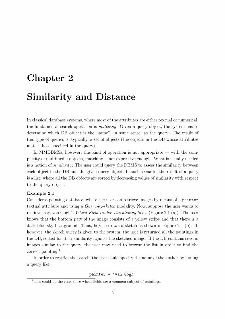
Consider a painting database, where the user can retrieve images by means of a painter
textual attribute and using a Query-by-sketch modality. Now, suppose the user wants to
retrieve, say, van Gogh’sWheat Field Under Threatening Skies (Figure 2.1 (a)). The user
knows that the bottom part of the image consists of a yellow stripe and that there is a
dark blue sky background. Thus, he/she draws a sketch as shown in Figure 2.1 (b). If,
however, the sketch query is given to the system, the user is returned all the paintings in
the DB, sorted for their similarity against the sketched image. If the DB contains several
images similar to the query, the user may need to browse the list in order to find the
correct painting.1
In order to restrict the search, the user could specify the name of the author by issuing
a query like
painter = ‘van Gogh’
1This could be the case, since wheat fields are a common subject of paintings.
5

6 Chapter 2. Similarity and Distance
(a) (b)
Figure 2.1: Van Gogh’s Wheat Field Under Threatening Skies (a) and the sketch of aquery to retrieve it (b).
Now the result of the query is a set of all van Gogh’s paintings. Again, since van Gogh
was a very prolific painter, the result set can consist of several images, that the user will
have to browse.
What the user has in mind, however, is a query like this:
(painter = ‘van Gogh’) and (image = sketch)
In this case, the system has to combine a set with a list: What is the result of such a
query? Obviously, the user wants to be returned with a list of all van Gogh’s paintings
sorted with respect to their similarity with the sketched image. If, however, the query
is a more complicated one, the answer may not be so intuitive.2 We will precise these
concepts later in Chapter 7. ✷
2.1 Similarity Search
We now formalize the basic similarity operations that a typical MMDBMS has to deal
with. In the following, for the sake of simplicity, we suppose that the database scheme
consists of a single collection C of objects. We will, thus, ignore the actual implementationof C, which, for our purposes, can be represented by a relation, a class, etc., or as acombination of such schemes. Objects (tuples) of C can be compared by means of a set ofrelevant features F .3 The values of each feature F ∈ F belong to a domain D = dom(F ).
2.1.1 Similarity Queries
We consider similarity predicates p all having the form F ∼ v, where F ∈ F is a feature,
v ∈ D is a constant value (the query value), and ∼ is a similarity operator. When applied2As an example, consider the query obtained by substituting the and operator with an or in the
previous query.3For instance, images can be compared using attributes like color, texture, shape, etc.
2.2 Similarity Theories 7
to an object O ∈ C, the predicate p returns a score (grade) s(p,O.F ) ∈ [0, 1], assessingthe similarity (with respect to feature F ) of object O to the query value v. Evaluating a
predicate p on all the objects of C, thus, yields a “graded set” {(O, s(p,O.F )) : O ∈ C}.For instance, evaluating the predicate color ∼ ‘red’ on an image DB means to assign
to each image in the collection a score assessing its “redness”. We can also think of a
graded set returned by a similarity predicate as corresponding to a sorted list, where the
objects of the collection C are sorted by their grades, i.e. by their similarity to the queryvalue.
The two basic form of similarity queries that we consider are range and nearest neigh-
bors queries.
Definition 2.1 (Range query)
Given a predicate p : F ∼ v and a minimum similarity threshold α, the (simple)
range query range(p, α, C) selects all the objects in C, along with their scores, such thats(p,O.F ) ≥ α, that is, all the objects whose grade with respect to p is not less than α. ✷
Definition 2.2 (Nearest neighbors query)
Given a predicate p : F ∼ v and an integer k ≥ 1, the (simple) nearest neighbor query
NN(p, k, C) selects the k objects in C, along with their scores, having the highest gradeswith respect to p, with ties arbitrarily broken. ✷
2.2 Similarity Theories
The concept of similarity has been widely investigated throughout the last century, both
in the field of psychology and in that of computer science, attempting to define a theory
consistent with the huge amount of experimental data. An important point, discovered by
computer scientists only in recent times [SJ98], is the discrepancy between the concepts of
similarity in psychology and in computer science. In computer science, usually, the simi-
larity has the target of recognizing an object under conditions of uncertainty. There is an
object and a model of the same object: The system has to assess if the actual appearance
of the object, different from the appearance of the model due to noise, distortion, etc.,
is consistent with the model itself. Computer scientists, thus, have to define the class of
possible transformations that an object can undergo.
The human concept of similarity is completely different: Human mind has to assess
the similarity between different objects. Thus, there is no way to define a number of
deformations to transform an object into another one.
It is, therefore, possible, for computer scientists, to assess the similarity between two
rotated images of a cube, since it is easy to model all the possible rotations of a cube in
8 Chapter 2. Similarity and Distance
the space, but the task of assessing the similarity between a cube and a tetrahedron is a
difficult one. And an even more difficult task is that of assessing if the image of a cube is
more similar to that of a tetrahedron or to that of a sphere.
The concept of similarity for our scenario is that of psychologists, since we want our
system to model the behavior of human mind in comparing perceptual stimuli. There-
fore, in the following, we will briefly review some of the similarity theories presented by
psychologists. Our goal is to obtain a concept of similarity sufficiently “close” to that of
human mind, but also useful for the purposes of searching in a database.
Psychologists usually distinguish between perceived similarity and judged similarity
[SJ98]. The judged similarity between two stimuli is usually defined as a real value in
the interval [0, 1], such that stimuli judged very similar by human mind have high judged
values. The most common definition of perceived similarity in psychology is that of a
distance function d assessing the dissimilarity between objects in a psychological space. If
A,B and C are objects and SA, SB and SC are the stimuli of such objects in a perceptual
space, usual features of d are the following (metric axioms):
d(SA, SA) = d(SB, SB) (constancy of self-similarity) (2.1)
d(SA, SB) ≥ d(SA, SA) (SA = SB) (minimality) (2.2)
d(SA, SB) = d(SB, SA) (symmetry) (2.3)
d(SA, SB) + d(SB, SC) ≥ d(SA, SC) (triangle inequality) (2.4)
Each of the previous properties, however, has been subject of debate by different
similarity theories. The axiom 2.1 of constancy of self-similarity has been refuted by
theories proposing that the dissimilarity between two stimuli in the perceptual space also
depends on the spatial density of objects around each stimulus, that is, human mind gives
higher self-similarity to stimuli that can be easily confused with other ones. The distance
function between stimuli SA and SB, thus, can be defined as:
d(SA, SB) = φ(SA, SB) + αh(SA) + βh(SB) (2.5)
where φ(SA, SB) is a function that satisfies the metric axioms and h(S) is the density of
stimuli around S. If φ(SA, SA) = 0, it is
d(SA, SA) = (α+ β)h(SA) (2.6)
thus self-similarity is not a constant and depends linearly on the density of stimuli around
the stimulus itself. This model emphasizes the fact that stimuli in “highly populated”
areas of the space have a higher self-similarity, because human mind seems to someway
“prototypize” such stimuli more than others.
2.3 Metric Spaces 9
Axiom 2.2 of minimality of the distance function has been refuted by different theories
of perception. These theories assert that sometimes an object is identified as another
object more frequently than it is identified as itself. Argumentations of such theories,
however, seem very feeble, thus the axiom of minimality appears to be well-founded to be
included in our considered similarity theory.
Axiom 2.3 states that the distance between stimuli is symmetrical. A number of the-
ories refuted this assumption, showing asymmetries between stimuli due to their different
“saliency”. What is observed is that, in general, the less salient stimulus is more similar
to the more salient than vice versa. The model of Equation 2.5 accounts for violation of
the symmetry assumption whenever α = β.
The last axiom 2.4 of triangle inequality is the most attacked assumption. It is,
however, the fundamental property that, as we will see in Chapter 4, allows us to organize
the collection of objects C to search it efficiently.As we have seen, all of the four basic assumptions for the distance function are (at least)
questionable. Our model of similarity, however, should be both effective (in the sense that
should effectively mimic the behavior of human mind in assessing similarity between two
stimuli) and efficient (in the sense that should efficiently organize the perceptual space in
order to answer to similarity queries). This tradeoff between effectiveness and efficiency
led us to consider only distance functions that satisfy all of the four metric axioms.
A last remark should be pointed out: The two kinds of similarity — judged and
perceived — are, obviously, inversely related, in the sense that high values of perceived
distance between two stimuli correspond to low values of judged similarity, and vice versa.
It should also be noted that only the judged similarity between two stimuli can be accessed
through experimentation.
2.3 Metric Spaces
Taking into account the considerations of Section 2.2, our scenario is the following: The
similarity s(vx, vy) between two feature values vx, vy ∈ D is assessed by means of a distancefunction d, satisfying the metric axioms, and of a correspondence function h, transforming
distance values (perceived similarities) into (judged) similarity scores. More precisely:
Definition 2.3 (Metric)
A metric function is a non-negative function d : D2 → �+0 such that, for each vx, vy, vz ∈

10 Chapter 2. Similarity and Distance
D, the following axioms are satisfied:
d(vx, vx) = 0 (non-negativity) (2.7)
d(vx, vy) > 0 (vx = vy) (positivity) (2.8)
d(vx, vy) = d(vy, vx) (symmetry) (2.9)
d(vx, vz) + d(vz, vy) ≥ d(vx, vy) (triangle inequality) (2.10)
✷
Relevant examples of metrics include, among others:
Example 2.2
The Minkowski (Lp) metrics over n-dimensional vector spaces, defined as Lp(vx, vy) =
(∑n
j=1 (|vx[j]− vy[j]|p)1/p (p ≥ 1). Special cases of such metrics are the Euclidean (L2)
and the Manhattan — or “city-block” — (L1) distances. When p → ∞, we obtain theL∞ metric defined as L∞(vx, vy) = maxnj=1 {|vx[j]− vy[j]|}. ✷
Example 2.3
The Levenshtein (edit) distance over strings, dE(s, t), which counts the minimum number
of edit operations (insertions, deletions, substitutions) needed to transform string s into
string t. ✷
Example 2.4
The Hausdorff metric over sets of points, which is used to compare 2-D shapes and is
defined as:
dH(Ox, Oy) = max{δ(Ox, Oy), h(Oy, Ox)}
where δ(Ox, Oy) = maximinj Lp(Ox,i, Oy,j) is the maximum Lp distance between a point
of Ox and any point of Oy. ✷
Example 2.5
The normalized overlap distance for set similarity, defined as
dno(Ox, Oy) = 1−‖Ox ∩Oy‖‖Ox ∪Oy‖
✷
Example 2.6
Quadratic-form distance functions are widely used in comparing images by means of their
color histograms [FEF+94, SK97]. In these cases, in fact, color histograms are represented
by n-dimensional points, but a Minkowski metric is not suitable for comparing such

2.3 Metric Spaces 11
vectors, since there is a correlation between the components (e.g. the color red is more
similar than the color green to the color orange).
The quadratic-form distance between histograms hx and hy is given by:
dQ(hx, hy) =√(hx − hy)TA(hx − hy)
where element Ai,j of the matrix denotes the similarity between the i-th and the j-th
colors of the histograms. ✷
The feature domain D and the metric d define a metric space M = (D, d). For ourpurposes, it is also convenient to assume that such a metric space is bounded, that is,
exists a finite d+ ∈ �+0 such that, for every vx, vy ∈ D, it is d(vx, vy) ≤ d+. This last
assumption is not essential, and we will only use it in Chapter 6.
In such a scenario, similarity queries defined in Section 2.1.1 can be rewritten as:
Definition 2.4 (Range query)
Given a collection C, a query value Q ∈ D, and a maximum distance threshold rQ, the
(simple) range query range(Q, rQ, C) selects all the objects in C such that d(O,Q) ≤ rQ,
that is, all the objects whose distance from Q does not exceed rQ. ✷
Definition 2.5 (Nearest neighbors query)
Given a collection C, a query value Q ∈ D, and an integer k ≥ 1, the (simple) nearest
neighbors query NN(Q, k, C) selects the k closest to Q objects in C, with ties arbitrarilybroken. ✷
The analogy between the definitions of similarity queries and distance queries is evi-
dent. These two parallel definitions manifest the correspondence between judged similar-
ity, used in similarity queries, and perceived similarity, used in distance queries. As we
saw in Section 2.2, there is an inverse relationship between these two concepts. This kind
of relationship is, in our scenario, materialized in the following
Definition 2.6 (Correspondence function)
A (distance to similarity) correspondence function is a function h : �+0 → [0, 1] having
the following properties:
h(0) = 1 (2.11)
x1 ≤ x2 ⇒ h(x1) ≥ h(x2) ∀x1, x2 ∈ �+0 (2.12)
✷
Intuitively, a correspondence function inversely relates similarity and distance (high dis-
tance values correspond to dissimilar objects and, thus, to low similarity scores) and
assigns the maximum similarity in case of 0 distance (exact-match).
12 Chapter 2. Similarity and Distance
2.4 Examples
In this Section we will review several approaches to similarity search in a variety of different
environments.
2.4.1 Image Retrieval
As we saw in Chapter 1, the use of textual descriptors to search through image databases
is largely inadequate. Usually, Image Storage and Retrieval (ISR) systems provide access
to content of images by means of image-analysis tools, extracting features like color,
shape and texture. Several systems, like Photobook [PPS96] from MIT, QBIC [FSN+95]
from IBM, Chabot [OS95], Virage [HGH+96], and VisualSEEk [SC96], all use Content
Based Visual Queries (CBVQs) to search in an image database. All these systems use
feature-based approaches to index images information.
Color Representation
The distribution of colors in an image is usually represented by an histogram. Each pixel
of an image I[x, y] consists of three color channels I = (IR, IG, IB), representing red,
green, and blue components. These channels are transformed, by way of a transformation
matrix Tc, into the natural components of color perception, that is, hue, brightness, and
saturation. Finally, the three latter channels are quantized, through a quantization matrix
Qc, into a space consisting of a finite number M of colors. The m-th component of the
histogram, hc[m] is given by:
hc[m] =∑x
∑y
{1 if Qc(TcI[x, y]) = m0 otherwise
(2.13)
Each image is, therefore, represented by a point in aM -dimensional space. To compare
histograms of different images, we can use a metric on such a space. Used metrics include
the Manhattan distance L1, the Euclidean distance L2, and the histogram quadratic
distance dQ of Example 2.6.
In [SO95], the authors propose an alternate method of color indexing. A 9-dimensional
vector, consisting of mean, variance, and skewness of the hue, saturation, and brightness
components for all the pixels, is extracted from each image. A method for preserving color
locality by dividing each image in 5 regions of fixed size and position, and by computing
the 9-dimensional vector for each of the 5 regions, thus obtaining a 45-dimensional vector
for each image, is also considered. On these vector, a weighted L1 metric (with weights
empirically computed) is then used to compare images. Though the authors claim that
2.4 Examples 13
their method is more efficient than others in finding images with the same content of
the query image, in [Smi97] it is shown that the simpler metrics (i.e. L1 and L2) provide
consistently better performance in retrieving images by color content.
In Appendix B, we describe a sample application of our approach to image retrieval
by color content.
Texture Representation
Textures are homogeneous patterns or spatial arrangements of pixels that cannot be
sufficiently described by regional intensity or color features. Texture for an image can be
represented, as for color, by an histogram. Image texture is first decomposed into nine
spatial-frequency subbands, by way of a wavelet filter bank. Then, a texture channel
generator is used to produce nine channels, starting from the nine subbands. Again,
these texture channels can be transformed (by way of a transformation matrix Tt) and
quantized (by way of a quantization matrixQt) to produce the final histogram representing
the image.
It is beyond the scope of this thesis to describe the mathematical tools used to produce
the texture channels from the original image. The only point that we like to emphasize
is that the histogram transformation is, typically, applied in order to provide invariance
with respect to rotation and scaling of the image.
The representation of texture as an histogram allows us to use, for texture similarity,
the same metrics used for color similarity. In particular, in [Smi97] it is shown that L1
and L2 metrics perform extremely well in retrieving images having texture similar to that
of the query image.
2.4.2 Content-Based Retrieval of Audio Data
Sounds are usually described by psychophysiologists using pitch, loudness, duration, and
timbre. While the former three physiological stimuli can be effectively modeled by measur-
able acoustic features, the timbre feature collects all those acoustic qualities of a sound
that cannot be represented by pitch, loudness and duration. In the light of what we
expressed in Section 2.2, the timbre feature has to be broken up into its principal com-
ponents. Salient elements of timbre include the amplitude and the spectral envelope, the
harmonicity, etc.
In [WBKW96], only four features — loudness, pitch, brightness, and bandwidth —
are used to classify and index sounds. However, since sounds have a duration, it is not
sufficient to use only a single value, since above features can vary over time. The average
value, the variance of the value over the duration of the signal, and the autocorrelation of
14 Chapter 2. Similarity and Distance
the trajectory over a small lag are computed for each of the four features and form, along
with the sound duration, the 13-dimensional vector used to index the sound space. The
vectors representing the relevant classes of sounds are then selected by an human expert.
The metric used in [WBKW96] to classify the sounds is a quadratic form distance having
the form:
dS(x, y) =√(x− y)TR(x− y)
where the matrix R is the inverse of the covariance matrix computed for the vectors
representing the classes. If the feature vector elements are reasonably independent of
each other, the off-diagonal elements of R can be ignored in the distance computations,
thus the metric assumes the form of a weighted L2 metric.
2.4.3 Face Recognition
Human and machine recognition of faces is a topic that has been subject of investigation by
psychophysicists over the last twenty years. The main issues of debate between scientists
are the following:
Is face recognition a dedicated process? That is, does exists a face recognition sys-
tem within the human brain? The existence of such system is supported by several
experiments (e.g. the fact that humans have difficulty in recognizing familiar faces
when these are presented upside down), thus experts usually agree on this topic.
Is face recognition the result of global or feature analysis? Most studies suggest
that human mind recognizes faces by using distinctive features (e.g. a big nose,
distant eyes, flapping ears, etc.). However, it is not clear what features are the most
distinctive for human recognition of faces.
What is the role of gender and/or race in the process of face recognition? It is
well known that humans recognize people from their own race better than people
from different races. It is also suspected that the recognition of male faces is slightly
different from that of female ones.
All these theories produced a number of different machine recognition systems. Several
approaches extract a number of numerical features from the face image (i.e. nose length
and width, mouth width and height, face width, chin radius, etc.) all normalized by the
interocular distance, in order to provide invariance to image scaling [BP93, KK72, Kan77].
These features form a multi-dimensional vector that is used to represent the corresponding
2.4 Examples 15
face. On this multi-dimensional vector space, a simple Manhattan or Euclidean metric is
then used to index the face space.
Another approach to face recognition uses the eigenvectors of the covariance matrix of
the set of database faces to find the principal components of the faces distribution [TP91].
The basic idea of this approach is the following: A face image of N ∗ N pixels may be
considered as a vector of dimension N2, thus a typical image is represented by a point in a
very high-dimensional space. Since face images are very similar in configuration, they will
be clustered in a relatively small area of the overall space, and, therefore, can be described
as points in a lower-dimensional subspace. The goal of Principal Component Analysis
(PCA), or Karhunen-Loeve (KL) expansion, is to find a suitable representation for this
subspace. Tipically, this is obtianed by extracting the k most significant eigenvectors of
the covariance matrix corresponding to the original face images. The value of the subspace
dimensionality, k, has to be high enough to be able to preserve the subspace topology (i.e.
different images are to be mapped to different points), but low enough to obtain a compact
representation of the subspace. Given the k most significant eigenvectors, the so-called
eigenfaces, each image is transformed to a point in the “face space” by projecting the
face onto the subspace defined by the eigenfaces. Usually the system uses an Euclidean
distance L2 as the metric in the face subspace. The system can now recognize faces by
using two distances:
• the distance ε between the image and its projection onto eigenfaces, describing thedistance of the image to the face space, and
• the minimum distance εk between the projection of the image and a point in the
subspace, corresponding to a face in the original dataset.
If the image is distant from the face space, then it is assumed that the image is not a face.
If the face is near to the face space and sufficiently near to a face image, then an individual
is recognized, otherwise the image is identified as the face of an unknown person. Both
recognizing tasks — that of recognizing the image as a face and that of recognizing a face
as a known person — use a threshold θ to define the maximum distance to the face space
and to an individual face.
2.4.4 Genomic Databases
A genomic database collects nucleotide sequences, i.e. DNA strings. Each string is com-
posed from a four-character alphabet of nucleotide bases, usually represented with letters
A, C, G, and T. An important kind of queries that can be issued to the system is the
16 Chapter 2. Similarity and Distance
local sequence alignment [WZ96]. Locally aligned DNA sequences are likely to behave in
a similar way. The score of local alignment for two DNA sequences x and y is given by:
s(x, y) = maxi{c · lengthi − gapsi} (2.14)
where c is a predefined constant, lengthi is the total length of alignment i, and gapsi is a
non-negative function that accounts for the gaps in the i-th alignment.
What is usually requested to the system is a set of sequences having a local alignment
score with respect to the query sequence q not lower than a given threshold σ, that is:
{x : s(x, q) ≥ σ} (2.15)
For all the sequences satisfying Equation 2.15, it exists an alignment j such that
c · lengthj ≥ σ (2.16)
The number of characters in the gaps is given by
‖x‖+ ‖q‖ − 2 · lengthj (2.17)
where ‖ · ‖ indicates the length of the string. The number of gaps is greater than or equalto the edit distance between the sequences, i.e. dE(x, q), when substitutions of characters
are not allowed. Thus, from Equations 2.15, 2.16, and 2.17, follows:
dE(x, q) ≤ ‖x‖+ ‖q‖ − 2σ/c (2.18)
A local alignment query, therefore, can be transformed into a distance range query with
non-constant radius r = ‖x‖+ ‖q‖ − 2σ/c [CA97].
Chapter 3
Indexing
In the previous Chapter, we discussed about the way of representing MM objects in order
to support similarity queries. We presented a generic approach, the feature extraction
technique, that can be used by a system to assess the similarity between two objects, by
exploiting a distance function. Now, we are faced with the problem of how to efficiently
deal with similarity queries.
If our MMDB has a relatively small size, e.g. in the order of hundreds of objects, and
the similarity function is computationally unexpensive, a sequential scan of the entire
database, followed by a similarity assessment, can be an adequate solution. However, as
the size of the database grows, or if the evaluation of similarity between two objects is a
non-trivial operation, the sequential scan of the database is not a reasonable arrangement.
What is needed is a way to filter out objects that are non-relevant to the query, without
dismissing relevant ones. Classical DBMSs use access methods, like indices and other
structures, to search through the objects of the database. Quoting from [SZ+96],
. . . Query processing will have to be extended to cover more data types
than those handled in today’s database products. For example, queries involv-
ing sequences (e.g. time series) are becoming more important. Optimization
over these structures will require new indexing methods and new query pro-
cessing strategies.
We have, hence, to find an access method suitable to index MM objects in the considered
similarity environment.
The requirements of modern multimedia applications call for access methods having
some fundamental features:
Dynamicity. The access structure has to support insertion and deletions of objects from
the database.
17
18 Chapter 3. Indexing
Scalability. Since the typical size of modern multimedia data repositories is in the order
of millions of objects, the access method should perform well also when the size of
the database grows.
Efficiency. Unlike typical access structures, which only try to minimize the number of
disk I/Os, indices for similarity search also have to take into account CPU costs,
since the task of computing the similarity between two objects can be computation-
ally very expensive.
Independence of the data. The access structure should have good performance for all
possible data distributions.
Use of secondary storage. Due to the huge amount of data, it is not conceivable to
store the entire dataset in main memory. The access structure, therefore, should be
able to efficiently exploit secondary (and possibly tertiary) storage devices.
In the previous Chapter, we assumed that our concept of similarity can be modeled
by means of a distance function on a suitable metric space. We also saw, through several
examples, that this metric space is, in most cases, indeed a vector space, on which a simple
Lp metric is used. In this scenario, similarity queries assume the form of spatial queries.
In order to deal with similarity queries in such spaces, an access method should implement
a clustering method — for grouping together similar objects — and a way to represent
such clusters for indexing purposes. This means that access structures used to index
classical tabular data, like B-trees, are not suitable to our goals. This is due to the lack
of ordering techniques, among multidimensional points, preserving space proximity. If we
try to extend one-dimensional access methods to multi-dimensional data, by sequentially
applying a structure to each dimension, the overall approach would be quite inefficient.
This is because each access method has to be independently traversed. The potentially
high selectivity on each dimension, therefore, cannot be exploited to restrict the search
in the remaining ones.
To support spatial search operation, what is needed is a multidimensional (or spatial)
access method. In recent times, a plethora of such methods has been proposed, each
claiming superior performance and/or generality with respect to others (for a survey, see
[Sam89, GG96]). In the following, we will review some of these Spatial Access Methods,
showing how they can be used to answer similarity queries.

3.1 Spatial Access Methods 19
3.1 Spatial Access Methods
Spatial Access Methods (SAMs) are access structures created to index points and ex-
tended objects (such as polyhedra) in a multidimensional vector space.1 Usually, points
corresponding to data objects are stored in buckets, each corresponding to a disk page.
Each bucket also defines a subspace of the overall vector space; such subspaces are often
refferred to as regions. In order to access the data buckets, a directory, corresponding to a
search tree or to a sort of hashing scheme, is provided. The directory implementation and
the region splitting algorithm are the distinctive characteristics that differentiate between
SAMs. In [SK88], the authors propose a classification taxonomy of SAMs, based on the
characteristics of the regions. Regions may:
• have rectilinear or arbitrarily polyhedral shape,
• cover the entire multidimensional space or just those parts containing data points,and
• overlap or be pairwise disjoint.
Common spatial database search operations include [GG96]:
Exact Match Queries. Find all the objects equal to the query object Q.
Point Queries. Find all the objects overlapping the query point Q.
Region Queries. Find all the objects with at least one point in common with the query
region Q.
Window Queries. Find all the objects with at least one point in common with the
hyper-rectangular query Q.
Containment Queries. Find all the objects containing the query region Q.
Enclosure Queries. Find all the objects enclosing the query region Q.
Adjacency Queries. Find all the objects adjacent to the query region Q.
Nearest Neighbor Queries. Find all the objects with a minimum distance from the
query object Q.
1Since stimuli are represented by points in a perceptual vector space, in the following we will ignoreextended objects, considering only punctual objects.
20 Chapter 3. Indexing
A study of topological relations that can be exploited in order to deal with such queries
with R-trees and similar access structures can be found in [PTSE95]. For our purposes,
however, the only interesting search operations that have to be supported by a SAM
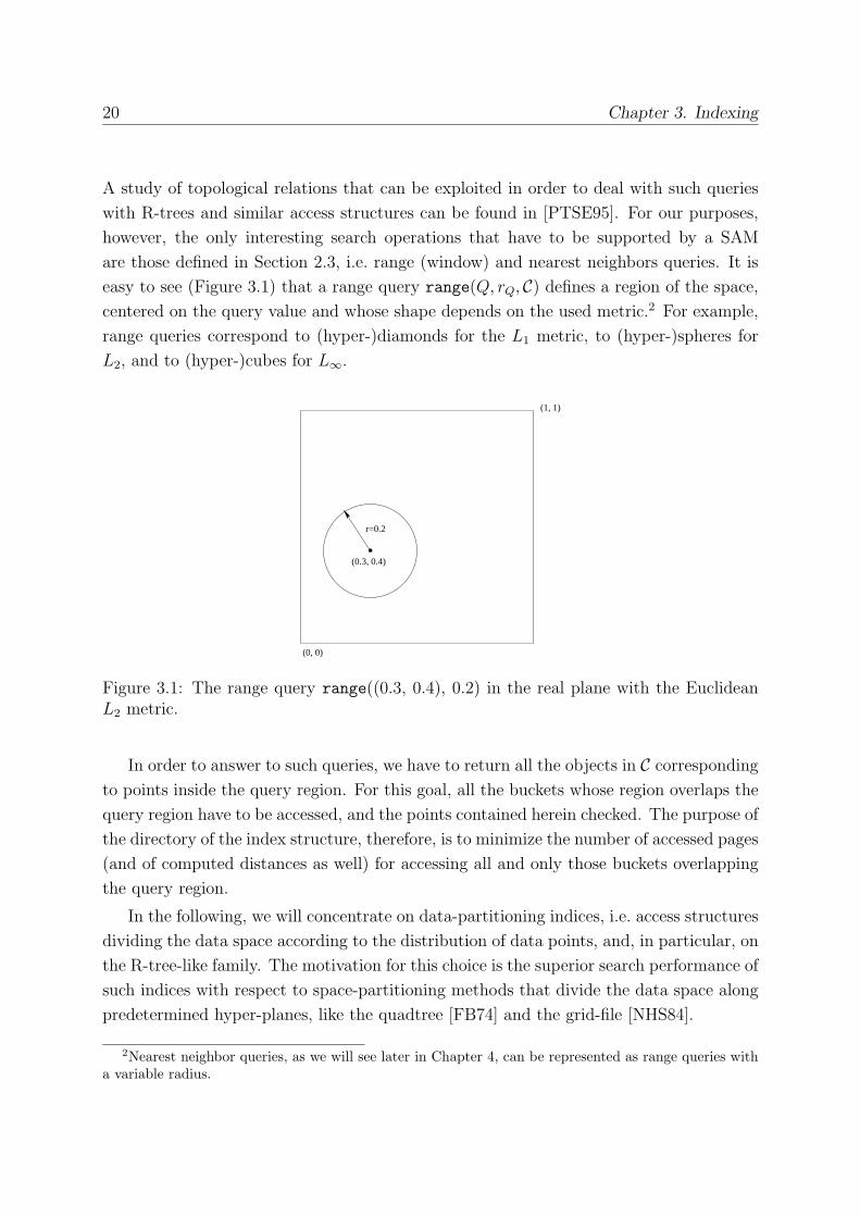
are those defined in Section 2.3, i.e. range (window) and nearest neighbors queries. It is
easy to see (Figure 3.1) that a range query range(Q, rQ, C) defines a region of the space,centered on the query value and whose shape depends on the used metric.2 For example,
range queries correspond to (hyper-)diamonds for the L1 metric, to (hyper-)spheres for
L2, and to (hyper-)cubes for L∞.
(1, 1)
(0, 0)
(0.3, 0.4)
r=0.2
Figure 3.1: The range query range((0.3, 0.4), 0.2) in the real plane with the EuclideanL2 metric.
In order to answer to such queries, we have to return all the objects in C correspondingto points inside the query region. For this goal, all the buckets whose region overlaps the
query region have to be accessed, and the points contained herein checked. The purpose of
the directory of the index structure, therefore, is to minimize the number of accessed pages
(and of computed distances as well) for accessing all and only those buckets overlapping
the query region.
In the following, we will concentrate on data-partitioning indices, i.e. access structures
dividing the data space according to the distribution of data points, and, in particular, on
the R-tree-like family. The motivation for this choice is the superior search performance of
such indices with respect to space-partitioning methods that divide the data space along
predetermined hyper-planes, like the quadtree [FB74] and the grid-file [NHS84].
2Nearest neighbor queries, as we will see later in Chapter 4, can be represented as range queries witha variable radius.
3.1 Spatial Access Methods 21
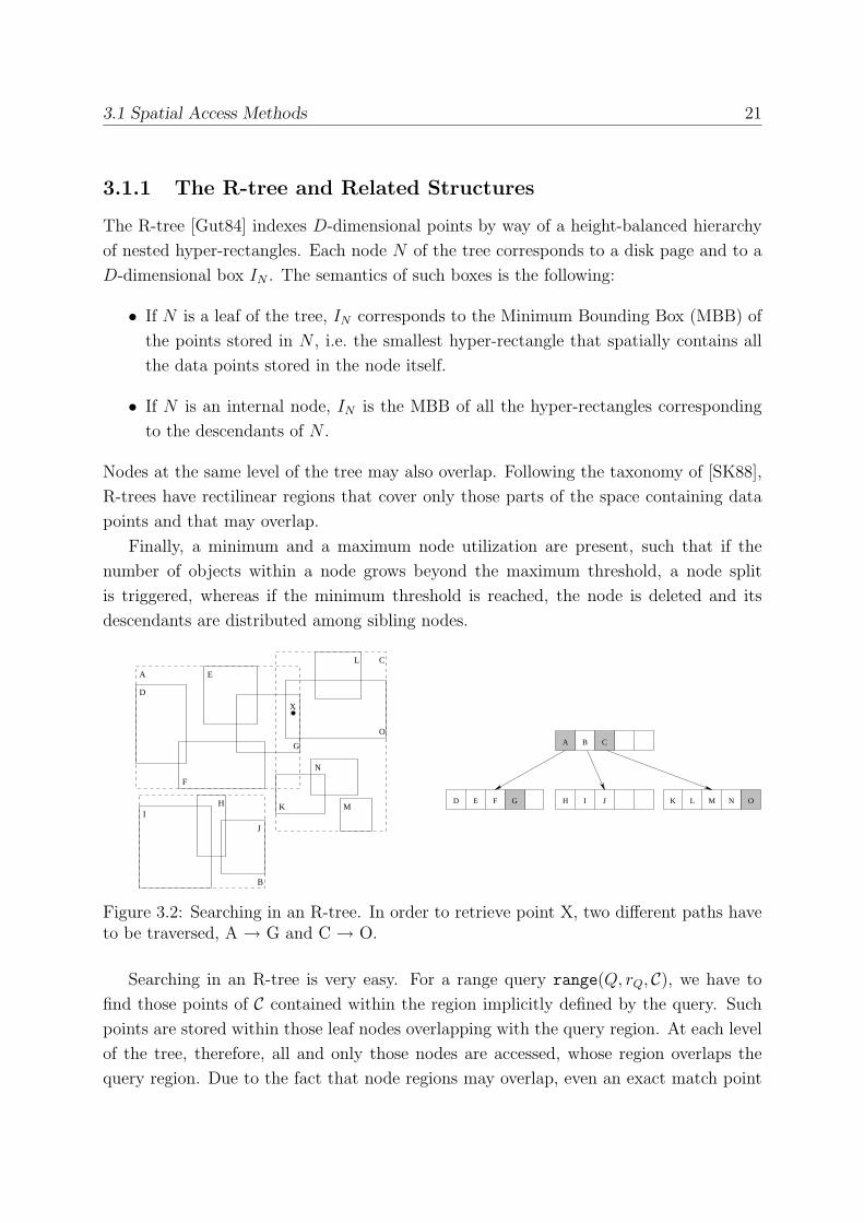
3.1.1 The R-tree and Related Structures
The R-tree [Gut84] indexes D-dimensional points by way of a height-balanced hierarchy
of nested hyper-rectangles. Each node N of the tree corresponds to a disk page and to a
D-dimensional box IN . The semantics of such boxes is the following:
• If N is a leaf of the tree, IN corresponds to the Minimum Bounding Box (MBB) of
the points stored in N , i.e. the smallest hyper-rectangle that spatially contains all
the data points stored in the node itself.
• If N is an internal node, IN is the MBB of all the hyper-rectangles corresponding
to the descendants of N .
Nodes at the same level of the tree may also overlap. Following the taxonomy of [SK88],
R-trees have rectilinear regions that cover only those parts of the space containing data
points and that may overlap.
Finally, a minimum and a maximum node utilization are present, such that if the
number of objects within a node grows beyond the maximum threshold, a node split
is triggered, whereas if the minimum threshold is reached, the node is deleted and its
descendants are distributed among sibling nodes.
X
IH
J
B
A
D
E
G
F
O
CL
N
K MD E F G H I J K L M N O
A B C
Figure 3.2: Searching in an R-tree. In order to retrieve point X, two different paths haveto be traversed, A → G and C → O.
Searching in an R-tree is very easy. For a range query range(Q, rQ, C), we have tofind those points of C contained within the region implicitly defined by the query. Suchpoints are stored within those leaf nodes overlapping with the query region. At each level
of the tree, therefore, all and only those nodes are accessed, whose region overlaps the
query region. Due to the fact that node regions may overlap, even an exact match point
22 Chapter 3. Indexing
query, i.e. a range query with radius equal to zero, may lead to multiple search paths
(see Figure 3.2). This fact, however, affects performance, introducing additional search
costs.3 In order to minimize search costs, in [Gut84] the author points out that the total
volume covered by the index regions has to be minimized. This is because, during the
search phase, a node is accessed only if its region overlaps the search region, thus smaller
nodes have a lower probability to be accessed. The goal of minimizing regions’ volume is
pursued during both the insertion and the node splitting phases:
• When inserting a new point in the index, at each level a node is chosen, for whichthe least volume enlargement of the corresponding region is needed. In case of ties,
the node corresponding to the smallest region is chosen.
• During splitting, the entries of the overflown node are to be divided into two nodes,with the goal of minimizing the volume of such nodes. Three algorithms are pro-
posed: An exhaustive algorithm, considering all possible groupings and choosing the
best one, and two quicker but non-optimal split algorithm, one having a quadratic
complexity in the number of entries and one with linear complexity.
Another cause of inefficiency, not considered in [Gut84], is the overlap of node regions,
leading to multiple paths searches. In [SRF87] the authors propose the R+-tree, an R-
tree-like structure that uses a clipping technique to overcome the problems caused by
overlaps. The main idea is that objects intersecting with more than one index region
have to be stored on multiple pages. The result of this technique is that a single path
traversal of the tree is needed to search for each point query. In case of range queries,
however, the index performance can even decrease, with respect to the original R-tree
organization, due to the objects replication leading to lower storage utilizations.
Another variant of the R-tree, the R∗-tree, is proposed in [BKSS90]. Following a thor-ough study of R-tree performance with different data distributions, the authors propose
two major modifications.
1. Instead of splitting an overflown node, the R∗-tree introduces the forced reinsertiontechnique: A number of entries is removed from the overflown node and reinserted
into the tree at the same level of the overflown node. The goal of this technique is to
achieve a dynamic reorganization of the tree. If a node is overflown after reinsertion,
it is split.
2. The other modification concerns the splitting phase. The original R-tree policy
only tries to minimize the overall regions volume. The authors introduce further
objectives for their splitting algorithm:3For SAMs, the only considered costs are typically I/O accesses.
3.1 Spatial Access Methods 23
• The overlap between node regions has to be minimized.
• The length of the regions’ perimeter should be minimized.
• The volume covered by internal nodes has to be minimized.
• Storage utilization should be maximized.
Comparison of experimental results show that the R∗-tree outperforms the R-tree as tosearch performance. This is the main reason for the world-wide success of this access
structure, which has been used in several DBMSs for spatial data.
In [KF94], the authors propose a new structure, the Hilbert R-tree, achieving a better
clustering of data within each node. This is obtained by using a space filling curve, namely
the Hilbert curve, associating an Hilbert Value to each point, and storing, within each
node N , the Largest Hilbert Value (LHV) of the data contained in the sub-tree rooted
at N . LHV is then used during the insertion phase to find the most suitable leaf node
in which the new entry is to be stored. Together with a revised split policy, the authors
claim superior performance with respect to R∗-tree.
The X-tree [BKK96] uses a different directory structure with respect to R-tree. The
authors claim that the main problem for R-tree-like structures is the overlap of the bound-
ing boxes in the directory, which grows as the dimensionality of the space increases. To
avoid this problem, a new splitting algorithm is introduced to minimize the overlap, to-
gether with the concept of super-nodes, i.e. variable size directory nodes, that can be read
faster with a sequential scan. The goal is to avoid splits of directory nodes that would
result in high overlaps. If there is no “good” split for an overflown node, the node is not
split and its size is extended by the size of a standard node. Experimental results show a
significant improvement over R∗-tree for space dimensionalities D ≥ 16.In [WJ96] the SS-tree is presented as a dynamic structure for similarity indexing. The
main difference with R-tree is that the SS-tree uses bounding hyper-spheres rather than
hyper-rectangles for the shape of nodes regions. Since a rectangle in a D-dimensional
space is defined by 2D values, i.e. the position of a pair of opposite vertices, whereas a
sphere is defined by the position of the center point and a radius, the fanout of a SS-tree
is higher than that of a R-tree. This can lead to better performance in high dimensional
spaces. However, search performance suffers from the high overlap between spheres and
the high volume of nodes regions.
To overcome the problems of the SS-tree, in [KS97] the SR-tree is proposed, using
intersections of spheres and rectangles as nodes regions. Each node, therefore, stores a
bounding hyper-sphere and a bounding hyper-rectangle, and the actual node region is
given by the intersection of the two. This reduces the overall volume of nodes regions
24 Chapter 3. Indexing
and the overlap in the directory, thus improving index performance during search phase.
However, since each node should store the definition of both a rectangle and a sphere, the
nodes fanout is considerably reduced, thus leading to a lower memory utilization.
3.1.2 The Curse of Dimensionality
All the presented methods for index multi-dimensional data have very bad performance in
high-dimensional spaces, i.e. when the space dimensionality is higher than, say, 20. What
is observed is that, even for range queries with very low selectivity, i.e. with very low
volume, all of the index nodes are accessed. This effect has been named, by researchers
in the area, the curse of dimensionality. In these cases, of course, a sequential scan of the
entire database has to be preferred. In order to understand the reasons for this behavior,
we first have to point out the fact that, for dimensions higher than 3, our intuition
completely fails, since we have no geometric view of the space. As an example, consider
the following situation:
Example 3.1
Suppose we have to draw, in the D-dimensional hyper-cube [0, 1]D, an hyper-sphere cen-
tered in the point p = (0.3, 0.3, . . . , 0.3) touching all the (D − 1)-surfaces of the space.The smallest of such spheres will have radius 0.7. We want to know if the center point
of the space cp = (0.5, 0.5, . . . , 0.5) is inside that sphere. Geometric intuition says that,
since the sphere touches every surface of the space, the center point will be included in
the hyper-sphere. For D = 16, however, it is L2(p, cp) =√∑16
i=1(0.5− 0.3)2 = 0.8, thusthe center point of the space is outside of the sphere. ✷
In [BBK98] it is shown that one of the major problems of R-tree-like indices is their
balanced split policy, It is known that, for low-dimensional spaces, it is advantageous to
have hyper-cubic regions, in order to minimize their perimeter [BKSS90]. To achieve such
goal, nodes are usually split in a balanced way, i.e. such that each new node contains
almost half of the data stored in the overflown node. What is observed is that the data
space cannot be split in every dimension. As an example, consider a 20-dimensional
space with data points uniformly distributed: Splitting the space at least once in each
dimension would lead to an index of 220 ≈ 1, 000, 000 leaf pages containing 20,000,000
objects, supposing an average storage utilization of 20 entries per page. Thus, with less
objects, the data space is split only on a number D′ < D of dimensions. Nodes regions
are, therefore, extended to the whole [0, 1] interval in D − D′ dimensions. This is alsoa major flaw of space-partitioning methods: If the space is divided along a number of
dimensions, the great majority of the partitions are empty.
3.2 Metric Trees 25
Another problem is given by the relation existing between the dimensionality of the
space and the radius of a range query. If we suppose an uniform distribution of data points
in the D-dimensional space, in order to achieve a certain selectivity s for the query, the
query radius rQ has to be chosen accordingly. For example, if we consider the L∞ metric,
the query radius rQ is given by
rQ =D√s/2
Thus, the query region would be an hyper-cube with side length q equal to 2rQ. For
D = 20 and s = 0.01%, it is q = 2rQ =20√0.0001 ≈ 0.63.
From the above consideration, it is easy to see that, in high-dimensional spaces, almost
every reasonable range query has to touch every page of the index. In [BBK98] this effect
is accurately modeled, showing that for D > 10 all of the pages of the index are accessed
during a range search. In [WSB98] it is shown that data-partitioning methods based on
hyper-rectangular regions, like R-tree and X-tree, and on hyper-spherical regions, like SS-
tree, degenerate if the dimensionality is higher than a certain threshold D. In this case,
all of the index nodes are acessed and, of course, a sequential scan of the dataset has to
be preferred. Analytical studies show that this threshold is reached for D ≈ 20.Another reason for the difficult indexing of high-dimensional spaces is the fact that,
for uniformly distributed datasets, almost every point is near a surface of the space. In
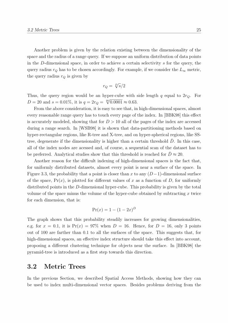
Figure 3.3, the probability that a point is closer than x to any (D−1)-dimensional surfaceof the space, Pr(x), is plotted for different values of x as a function of D, for uniformly
distributed points in the D-dimensional hyper-cube. This probability is given by the total
volume of the space minus the volume of the hyper-cube obtained by subtracting x twice
for each dimension, that is:
Pr(x) = 1− (1− 2x)D
The graph shows that this probability steadily increases for growing dimensionalities,
e.g. for x = 0.1, it is Pr(x) = 97% when D = 16. Hence, for D = 16, only 3 points
out of 100 are farther than 0.1 to all the surfaces of the space. This suggests that, for
high-dimensional spaces, an effective index structure should take this effect into account,
proposing a different clustering technique for objects near the surface. In [BBK98] the
pyramid-tree is introduced as a first step towards this direction.
3.2 Metric Trees
In the previous Section, we described Spatial Access Methods, showing how they can
be used to index multi-dimensional vector spaces. Besides problems deriving from the
26 Chapter 3. Indexing
0
0.1
0.2
0.3
0.4
0.5
0.6
0.7
0.8
0.9
1
0 5 10 15 20 25 30 35 40 45 50
Pro
babi
lity
Dim
x=0.05x=0.1
x=0.15x=0.2
Figure 3.3: The probability Pr(x) that a point is closer than x to any surface of the space,as a function of the space dimensionality.
so called dimensionality curse, two major issues prevent the use of SAMs for generic
similarity search environments:
1. We showed, in Section 3.1, that, in order to retrieve all the objects satisfying a
generic range query, all of the index nodes overlapping the query region are to be
accessed. Assessing if two regions overlap is an easy task if the used metric is a
simple one, but can be very difficult if the metric is complex, e.g. a quadratic form
distance.
2. SAMs can only index multi-dimensional vector spaces; thus, they are completely
useless for those environments where similarity between objects is assessed by means
of a non-vectorial distance function, e.g. for genomic databases (see Section 2.4.4).
3. When considering SAM performance, only I/O costs are considered, and CPU costs
ignored, on the assumption that the comparison between two points is not compu-
tationally expensive. In cases where this assumption is not true, e.g. in very high
dimensional spaces, the computation of the distance function cannot be ignored.
An additional optimization is therefore needed, in order to minimize the number of
computed distances.
The first of these problems can be overcome by using a lower bounding distance function
[SK98].
3.2 Metric Trees 27
Definition 3.1 (Lower bounding distance function)
If dO : D2 → �+0 is a (complex) distance function, we say that df : D2 → �+
0 is a lower
bounding distance function of dO (df ≤ dO), if df is an underestimate of dO, that is:
df (vx, vy) ≤ dO(vx, vy) ∀vx, vy ∈ D
✷
The basic idea is to use a simple distance function (e.g. a Minkowski metric) as an
approximation of the “real” distance function. In such cases, in order to answer to a range
query, the index is searched using the lower bounding distance. Then, all and only those
objects contained in the result of the query are exactly evaluated against the query value
through a refinement filtering step, using the real distance.4
The lower bounding property is essential to prevent false dismissals, i.e. objects satis-
fying the query but not returned in the result. Of course, indexing the space is useful only
if the lower bound is “tight”, i.e. if the approximating distance is sufficiently close to the
real distance for every pair of objects. Otherwise, the cardinality of the candidates set,
i.e. the set returned by the index search phase, would be very high and the filtering step
will compute the complex distance between the query value and almost all the objects of
the dataset. Obviously, in this case a sequential scan of the database would be a quicker
solution.
The second problem for SAMs can be solved in a similar manner. It is, however,
very difficult to find a lower bounding distance function for arbitrarily complex metrics.
Moreover, some metrics have to be mapped to very high-dimensional spaces, where SAMs
are completely uneffective, as we saw in Section 3.1.2. As an example, consider the edit
distance between strings. This metric can be approximated by a vector distance function
in a space whose dimensionality is proportional to the length of the indexed strings. In
genomic DBs, proteic sequences can be composed of hundreds of terms, thus the target
vector space will have a very high dimensionality, well beyond the threshold for the
usefulness of SAMs.
These considerations led to the development of metric trees [Uhl91]. A generic defini-
tion for a metric tree is the following:
Definition 3.2 (Metric tree)
A metric tree is an index structure having the following characteristics:
1. Leaf nodes store (pointers to) the data objects.
4A similar, but more complex, procedure is used for nearest neighbor queries; an optimal algorithmis presented in [SK98].
28 Chapter 3. Indexing
2. A region of the space is associated to each node.
3. The region associated with the root node corresponds to the whole space.
4. Regions associated to the children nodes of node N are enclosed in the region asso-
ciated to node N .
5. The region associated with node N is such that all the objects stored in the sub-tree
rooted at node N are contained within the region itself.
✷
Regardless of the specific space partitioning algorithm, metric trees aim at grouping to-
gether objects that are close to each other and at separating distant objects.
Searching in a metric tree involves accessing all the nodes whose sub-tree could store
objects contained in the region associated with the query. How this task has to be
accomplished depends on the space decomposition of the considered metric tree.
In [Uhl91], the author points out two different decompositions of a metric space:
1. the ball decomposition, and
2. the generalized hyperplane decomposition.
In the ball decomposition, the space is dissected using a single object v. The regions
associated with nodes correspond to spherical cuts around v. In the generalized hyper-
plane decomposition, the space is broken up using two different objects vx and vy. The
generalized hyperplane (GH) between the two points is defined as the set of objects v
satisfying the equation d(vx, v) = d(vy, v). The two regions, thus, are defined as the set
of points that are closer to one object than to the other. These two methods originated
several index structures that we outline in the following sections.
3.2.1 The vp-tree
The vantage-point tree, proposed in [Yia93], is based on the ball decomposition strategy;
therefore, the space is decomposed using spherical cuts around so-called vantage points.
In a binary vp-tree, each internal node has the format [Ov, µ, ptrl, ptrr], where Ov is the
vantage point (i.e. an object of the dataset chosen using a specific algorithm), µ is (an
estimate of) the median of the distances between Ov and all the objects reachable from
the node, and ptrl and ptrr are pointers to the left and right child, respectively. The left
child of the node indexes the objects whose distance from Ov is less than or equal to µ,
while the right child indexes the objects whose distance from Ov is greater than µ. The
3.2 Metric Trees 29
same principle is recursively applied to the lower levels of the tree, leading to an almost
balanced index.
The search algorithm for a range query range(Q, rQ, C) is the following:
1. If d(Q,Ov) ≤ rQ, then insert Ov in the result set.
2. If d(Q,Ov) + r ≥ µ, then recursively search in the node pointed by ptrr (right
branch).
3. If d(Q,Ov)−r ≤ µ, then recursively search in the node pointed by ptrl (left branch).
In [Chi94] the vp-tree structure is enhanced to deal with nearest neighbor queries.
The binary vp-tree can be easily generalized into a multi-way vp-tree, having nodes
with a higher fanout, by partitioning the distance values between the vantage point and
the data objects into m groups of (almost) equal cardinality. Then, the distance values
µ1, . . . , µm−1 used to partition the set are stored within each node, replacing the median
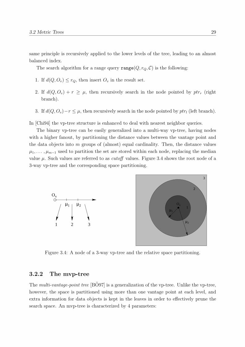
value µ. Such values are referred to as cutoff values. Figure 3.4 shows the root node of a
3-way vp-tree and the corresponding space partitioning.
2µ1µ
Ov
1 2 3µ2
v
µ
O
11
3
2
Figure 3.4: A node of a 3-way vp-tree and the relative space partitioning.
3.2.2 The mvp-tree
The multi-vantage-point tree [BO97] is a generalization of the vp-tree. Unlike the vp-tree,
however, the space is partitioned using more than one vantage point at each level, and
extra information for data objects is kept in the leaves in order to effectively prune the
search space. An mvp-tree is characterized by 4 parameters:

30 Chapter 3. Indexing
1. the number of vantage points in every node (in [BO97] only 2 vantage points are
considered),
2. the number of partitions created by each vantage point (v),
3. the maximum capacity of leaf nodes (f), and
4. the number of distances to be stored for the data objects at leaves’ level (p).
In each node of the mvp-tree, the first vantage point divides the space into v parts
using v − 1 cutoff values, while the second vantage point divides each of these parts inv partitions, using v − 1 cutoff values for each partition. In Figure 3.5 it is shown howa spherical shell partition can be split using a different vantage point. To partition the
space in v spherical cuts, the data objects are ordered with respect to their distances from
the vantage point, and then divided in v groups of (almost) equal cardinality. The v − 1distance values used to partition the data space (the cutoff values) are stored in each
internal node of the tree. The v2 groups of data objects are, then, recursively indexed by
the v2 children of the root node. The fanout of each node, thus, is v2 (in general, it is v
to the power of the number of vantage points).
1
3
2
2
vp
Figure 3.5: How a spherical shell partition can be split using a different vantage point.
The leaf nodes of the tree store the exact distances between the f data objects and
the 2 vantage points of that leaf, as well as the f · p distances between each data object xand the first p vantage points along the path from the root to the leaf node containing x.
During the construction phase, at each level, the first vantage point is chosen randomly,
while the second vantage point is the farthest object from the first vantage point. This,
as stated in [Sha77], increases the effectiveness of the data space partitioning during the
search phase.
3.2 Metric Trees 31
The search algorithm for the mvp-tree is similar to that of the vp-tree, but the cutoff
values for both vantage points in every node are used to prune the search and to avoid
distance computations.
3.2.3 The gh-tree
The generalized hyperplane tree is based on the GH decomposition proposed in [Uhl91].
For each node of the tree, two objects are chosen. Then, the remaining objects are
partitioned, based on which of the two chosen objects they are closer to. Again, the same
principle is recursively applied to lower levels of the tree.
The major limitations of this structure is the low fanout of each node, which is limited
to two, and the fact that the structure tends to be unbalanced.
3.2.4 The GNAT
To overcome the low fanout problem of gh-trees, in [Bri95] the Geometric Near-neighbor
Access Tree (GNAT) was proposed, which is based on the concept of Dirichlet domains.5
At each level of the tree, k split points {x1, . . . , xk} from the dataset are chosen.
The remaining objects in the dataset are then divided into the k Dirichlet domains
Dxi(i = 1, . . . , k) of the split points. For each pair of split points (xi, xj) the interval
range(xi, Dxj) = [mind(xi, Dxj
),maxd(xi, Dxj)] is computed, representing the minimum
and the maximum of d(xi, x), ∀x ∈ Dxj∪ {xj}. The same approach is then recursively
applied to each Dxi, possibly using a different value for k, the node degree, in order to
obtain a height-balanced tree. Figure 3.6 shows a sample GNAT.
For a range query range(Q, rQ, C), the GNAT is recursively searched in the followingway:
1. Let P represent the set of split points in the current node.
2. Choose a point xi from P (never the same one twice); if d(Q, xi) ≤ rQ, add xi to
the result.
3. ∀xj ∈ P , if [d(Q, xi)− r, d(Q, xi) + r, ]∩ range(xi, Dxj) = ∅, remove xj from P .
4. Repeat steps 2. and 3. until all the objects in P have been tried.
5. ∀xj ∈ P , recursively search Dxj.
5Given a set of points {x1, . . . , xk}, the Dirichlet domain of xi consists of all possible objects of thespace wich are closer to xi than to any other point xj(j = i).
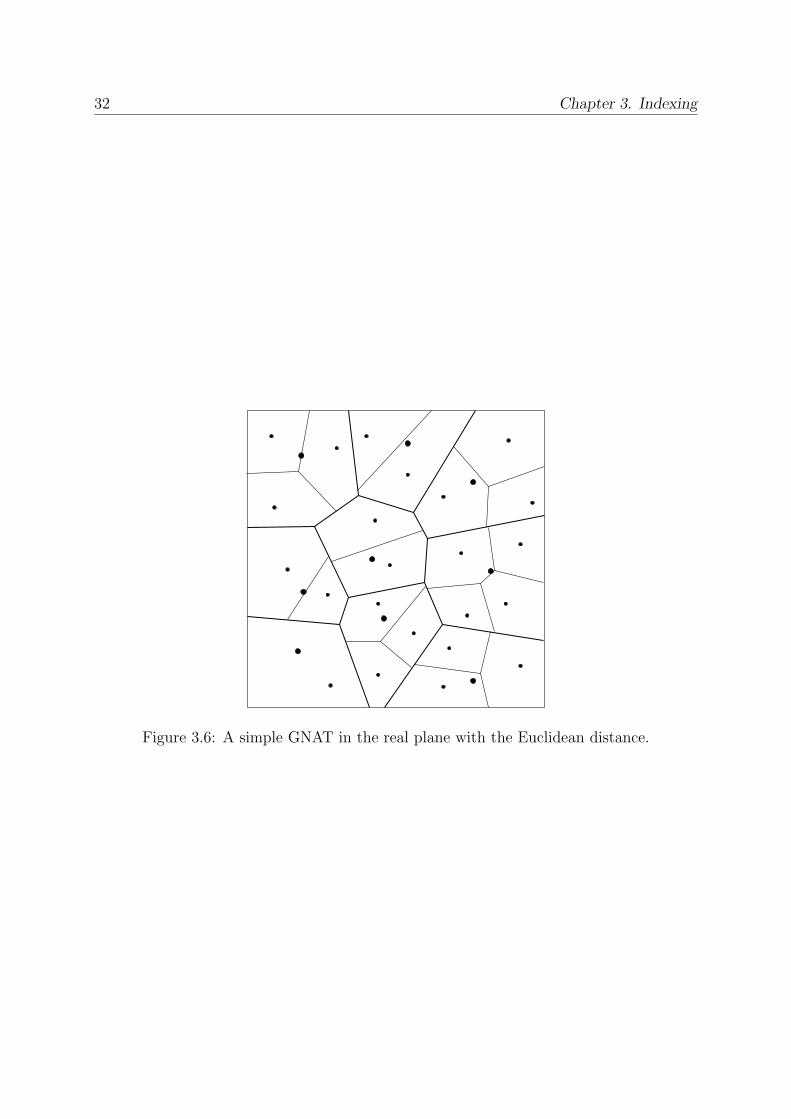
32 Chapter 3. Indexing
Figure 3.6: A simple GNAT in the real plane with the Euclidean distance.

Chapter 4
The M-tree
In the previous Chapter, we pointed out the required features for an access structure that
would have to deal with similarity queries in a MMDBMS, i.e. dinamicity, scalability,
efficiency, independence of the data, and use of secondary storage. All the access structure
that we reviewed in the previous Chapter, however, fail the test:
• SAMs have good properties of dinamicity and scalability, and efficiently exploitsecondary storage devices, but are restricted to vector spaces.
• Some metric trees, like vp- and mvp-trees, are balanced, hence providing a goodscalability, but are static, since they are built in a top-down manner.
• Other metric indices, like GNAT, are, at least in principle, dynamic but not bal-anced.
• Moreover, all known metric trees are memory-resident and do not use secondarystorage.
To overcome these problems, in [CPZ97] we presented the M-tree, a dynamic, paged,
and height-balanced metric tree.
4.1 Basic Principles
The M-tree organizes the objects into fixed-size nodes.1 Each node can store up to M
entries — this is the capacity of M-tree nodes. (The features of) DB objects are stored into
leaf nodes, whereas internal nodes store the so-called routing objects. A routing object
is a database object to which a routing role is assigned by a specific, called promotion,
1Nothing would prevent using variable-size nodes, a la X-tree [BKK96]. For simplicity, however, wedo not consider this possibility here.
33
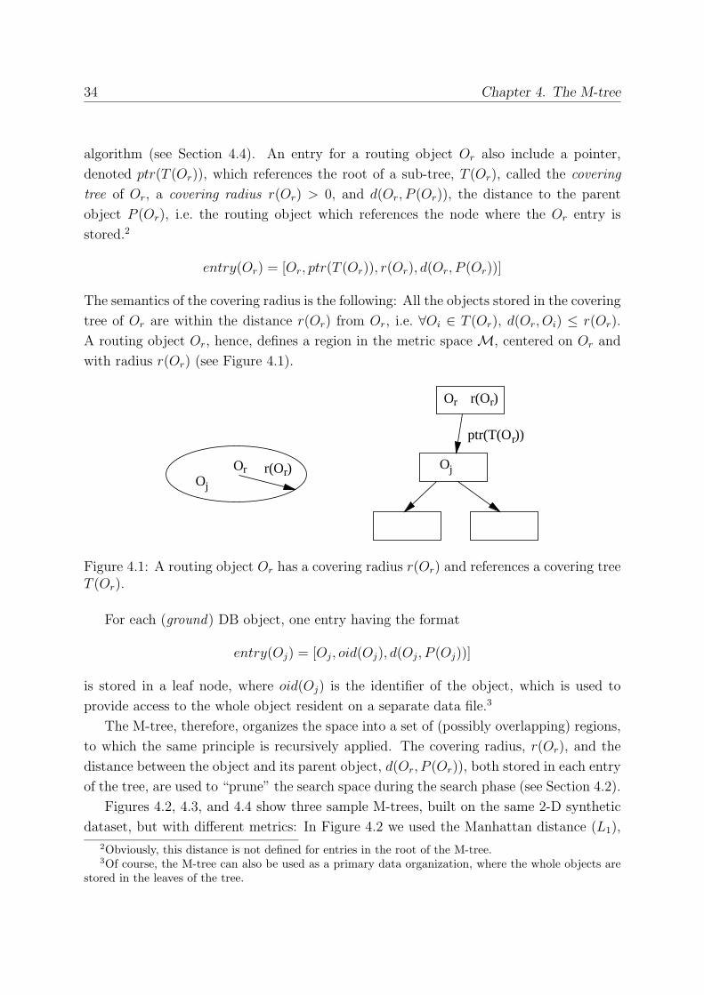
34 Chapter 4. The M-tree
algorithm (see Section 4.4). An entry for a routing object Or also include a pointer,
denoted ptr(T (Or)), which references the root of a sub-tree, T (Or), called the covering
tree of Or, a covering radius r(Or) > 0, and d(Or, P (Or)), the distance to the parent
object P (Or), i.e. the routing object which references the node where the Or entry is
stored.2
entry(Or) = [Or, ptr(T (Or)), r(Or), d(Or, P (Or))]
The semantics of the covering radius is the following: All the objects stored in the covering
tree of Or are within the distance r(Or) from Or, i.e. ∀Oi ∈ T (Or), d(Or, Oi) ≤ r(Or).
A routing object Or, hence, defines a region in the metric spaceM, centered on Or and
with radius r(Or) (see Figure 4.1).
Or r(O )r
Or r(O )r
Oj
Oj
ptr(T(O ))r
Figure 4.1: A routing object Or has a covering radius r(Or) and references a covering treeT (Or).
For each (ground) DB object, one entry having the format
entry(Oj) = [Oj, oid(Oj), d(Oj, P (Oj))]
is stored in a leaf node, where oid(Oj) is the identifier of the object, which is used to
provide access to the whole object resident on a separate data file.3
The M-tree, therefore, organizes the space into a set of (possibly overlapping) regions,
to which the same principle is recursively applied. The covering radius, r(Or), and the
distance between the object and its parent object, d(Or, P (Or)), both stored in each entry
of the tree, are used to “prune” the search space during the search phase (see Section 4.2).
Figures 4.2, 4.3, and 4.4 show three sample M-trees, built on the same 2-D synthetic
dataset, but with different metrics: In Figure 4.2 we used the Manhattan distance (L1),
2Obviously, this distance is not defined for entries in the root of the M-tree.3Of course, the M-tree can also be used as a primary data organization, where the whole objects are
stored in the leaves of the tree.

4.2 Searching the M-tree 35
for Figure 4.3 we used the Euclidean distance (L2), while in Figure 4.4 we used the L∞metric. Green regions correspond to leaf nodes whereas level 1 nodes are shown in red.
Figure 4.2: A sample M-tree on the [0, 1]2 domain with the L1 distance.
4.2 Searching the M-tree
Before presenting specific algorithms for building the M-tree, we show how the information
stored in nodes is used for processing similarity queries. Clearly, the performance of search
algorithms is largely influenced by the actual construction of the M-tree, even though the
correctness and the logic of search are independent of such aspects.
In order to minimize both the number of accessed nodes and computed distances,
all the information concerning (pre-computed) distances which are stored in the M-tree
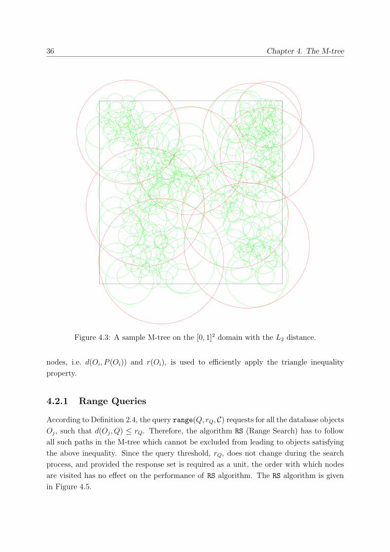
36 Chapter 4. The M-tree
Figure 4.3: A sample M-tree on the [0, 1]2 domain with the L2 distance.
nodes, i.e. d(Oi, P (Oi)) and r(Oi), is used to efficiently apply the triangle inequality
property.
4.2.1 Range Queries
According to Definition 2.4, the query range(Q, rQ, C) requests for all the database objectsOj, such that d(Oj, Q) ≤ rQ. Therefore, the algorithm RS (Range Search) has to follow
all such paths in the M-tree which cannot be excluded from leading to objects satisfying
the above inequality. Since the query threshold, rQ, does not change during the search
process, and provided the response set is required as a unit, the order with which nodes
are visited has no effect on the performance of RS algorithm. The RS algorithm is given
in Figure 4.5.
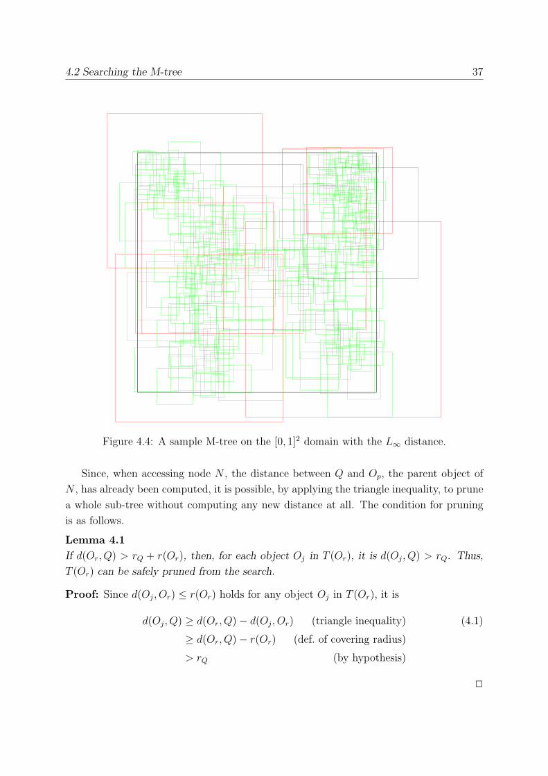
4.2 Searching the M-tree 37
Figure 4.4: A sample M-tree on the [0, 1]2 domain with the L∞ distance.
Since, when accessing node N , the distance between Q and Op, the parent object of
N , has already been computed, it is possible, by applying the triangle inequality, to prune
a whole sub-tree without computing any new distance at all. The condition for pruning
is as follows.
Lemma 4.1
If d(Or, Q) > rQ + r(Or), then, for each object Oj in T (Or), it is d(Oj, Q) > rQ. Thus,
T (Or) can be safely pruned from the search.
Proof: Since d(Oj, Or) ≤ r(Or) holds for any object Oj in T (Or), it is
d(Oj, Q) ≥ d(Or, Q)− d(Oj, Or) (triangle inequality) (4.1)
≥ d(Or, Q)− r(Or) (def. of covering radius)
> rQ (by hypothesis)
✷
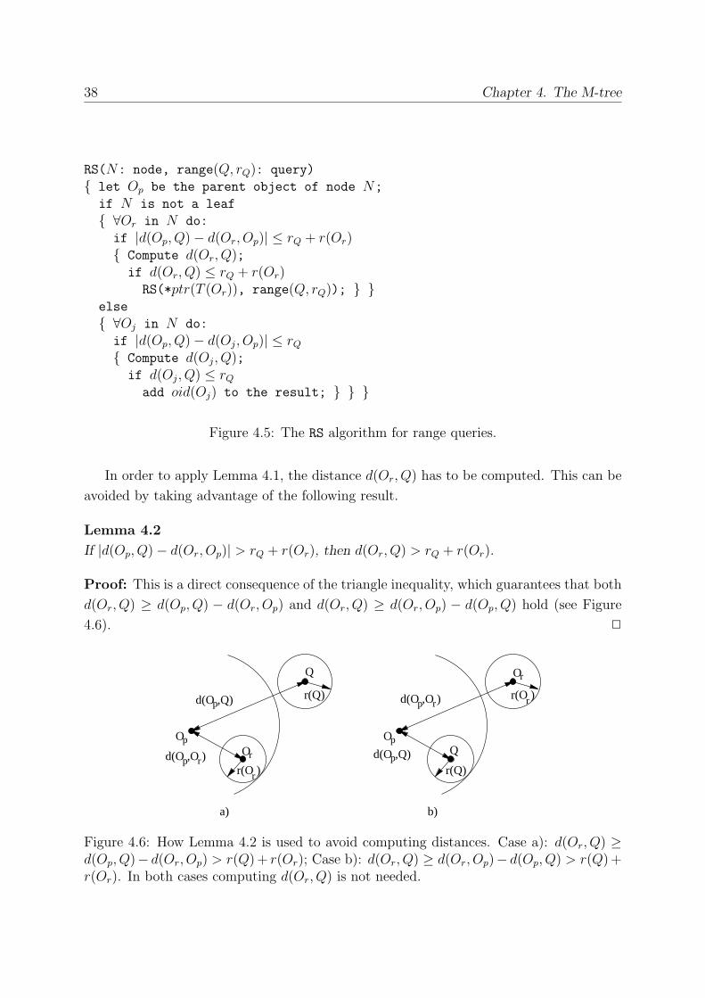
38 Chapter 4. The M-tree
RS(N: node, range(Q, rQ): query)
{ let Op be the parent object of node N;
if N is not a leaf
{ ∀Or in N do:
if |d(Op, Q)− d(Or, Op)| ≤ rQ + r(Or){ Compute d(Or, Q);if d(Or, Q) ≤ rQ + r(Or)RS(*ptr(T (Or)), range(Q, rQ)); } }
else
{ ∀Oj in N do:
if |d(Op, Q)− d(Oj, Op)| ≤ rQ{ Compute d(Oj, Q);if d(Oj, Q) ≤ rQadd oid(Oj) to the result; } } }
Figure 4.5: The RS algorithm for range queries.
In order to apply Lemma 4.1, the distance d(Or, Q) has to be computed. This can be
avoided by taking advantage of the following result.
Lemma 4.2
If |d(Op, Q)− d(Or, Op)| > rQ + r(Or), then d(Or, Q) > rQ + r(Or).
Proof: This is a direct consequence of the triangle inequality, which guarantees that both
d(Or, Q) ≥ d(Op, Q) − d(Or, Op) and d(Or, Q) ≥ d(Or, Op) − d(Op, Q) hold (see Figure
4.6). ✷
r(O )r
Ord(O ,O )p r
Op
d(O ,Q)p
Q
r(Q)
a)
Op
d(O ,Q)p
d(O ,O )p r
rO
r(O )r
b)
Q
r(Q)
Figure 4.6: How Lemma 4.2 is used to avoid computing distances. Case a): d(Or, Q) ≥d(Op, Q)− d(Or, Op) > r(Q)+ r(Or); Case b): d(Or, Q) ≥ d(Or, Op)− d(Op, Q) > r(Q)+r(Or). In both cases computing d(Or, Q) is not needed.
4.2 Searching the M-tree 39
Experimental results (see Section 4.7.7) show that this technique can save up to 40%
distance computations. The only case where distance are necessarily computed is when
dealing with the root node of the M-tree, for which Op is undefined.
4.2.2 Nearest Neighbor Queries
Given a k-nearest neighbors query NN(Q, k, C), the k-NN Search algorithm retrieves the
k nearest neighbors of the query object Q — it is assumed that at least k objects are
indexed by the M-tree. The steps of the k-NN Search algorithm closely resemble those of
the RS algorithm. However, since the pruning criterion of k-NN Search is dynamic (i.e.
the current search radius is determined by the distance between Q and the k-th nearest
neighbor at a given moment), specific attention should be paid to the order in which the
nodes are visited. Intuitively, if k objects “very close” to Q are found in the first stages of
the search, performance improves since the likelihood that more sub-trees can be pruned
increases significantly. As we saw before, the conditions which allow to avoid computing
a distance and accessing a node both require the search radius to be as small as possible.
We use a branch-and-bound technique, quite similar to the one designed for R-trees
[RKV95], which utilizes two global structures: A priority queue, PR, of pending requests,
and a k-elements array, NN, which, at the end of execution, contains the result.
Each entry in the PR queue is a pair (ptr(T (Or)), dmin(T (Or))). The first field is, as
in algorithm RS, the pointer to (the root of) sub-tree T (Or), whereas the second field is a
lower bound on the distance between Q and any object Oj in T (Or), that is:
dmin(T (Or)) ≤ d(Oj, Q) ∀Oj ∈ T (Or)
Clearly, the dmin(T (Or)) lower bound is given by:
dmin(T (Or)) = max{d(Or, Q)− r(Or), 0}
since no object in T (Or) can have a distance from Q less than d(Or, Q) − r(Or). These
bounds are used by the ChooseNode function to extract the next node to be examined
from the PR queue. The heuristic criterion implemented by the ChooseNode function is
to select the node for which the dmin lower bound is minimum.
At the end of execution, the i-th entry of the NN vector contains the pair (oid(Oj), d(Oj, Q)),
where Oj is the i-th nearest neighbor of Q. The distance value in the i-th entry is also
denoted as di (thus dk is the largest distance value in NN). Clearly, dk can be seen as
a dynamic search radius, since any sub-tree for which dmin(T (Or)) ≥ dk can be safely
pruned.
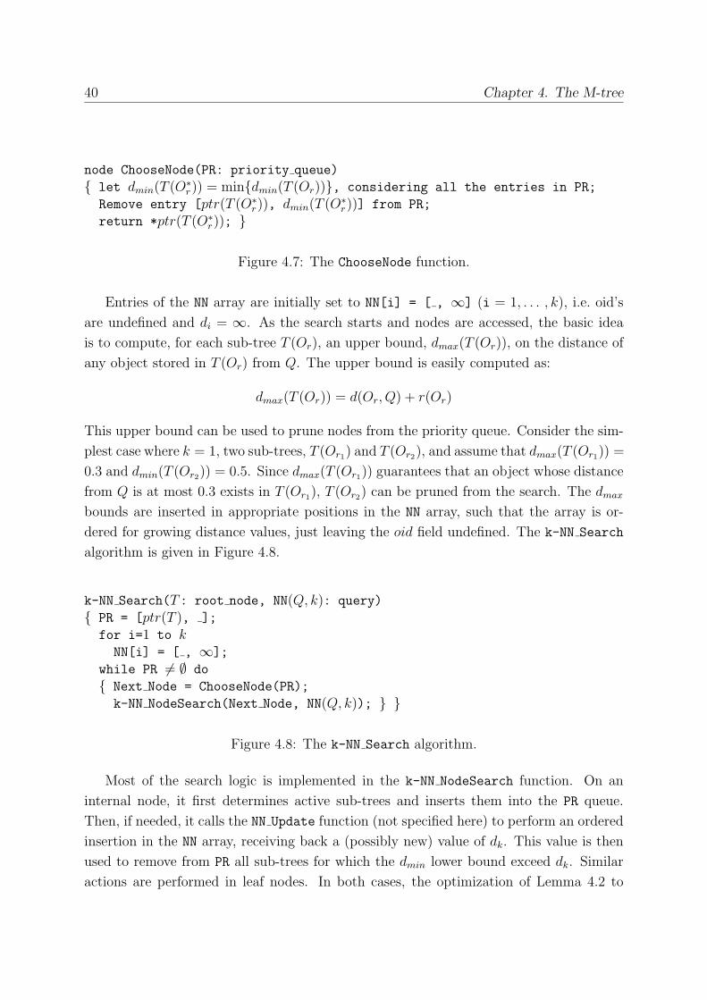
40 Chapter 4. The M-tree
node ChooseNode(PR: priority queue)
{ let dmin(T (O∗r)) = min{dmin(T (Or))}, considering all the entries in PR;
Remove entry [ptr(T (O∗r)), dmin(T (O
∗r))] from PR;
return *ptr(T (O∗r)); }
Figure 4.7: The ChooseNode function.
Entries of the NN array are initially set to NN[i] = [ , ∞] (i = 1, . . . , k), i.e. oid’s
are undefined and di = ∞. As the search starts and nodes are accessed, the basic ideais to compute, for each sub-tree T (Or), an upper bound, dmax(T (Or)), on the distance of
any object stored in T (Or) from Q. The upper bound is easily computed as:
dmax(T (Or)) = d(Or, Q) + r(Or)
This upper bound can be used to prune nodes from the priority queue. Consider the sim-
plest case where k = 1, two sub-trees, T (Or1) and T (Or2), and assume that dmax(T (Or1)) =
0.3 and dmin(T (Or2)) = 0.5. Since dmax(T (Or1)) guarantees that an object whose distance
from Q is at most 0.3 exists in T (Or1), T (Or2) can be pruned from the search. The dmax
bounds are inserted in appropriate positions in the NN array, such that the array is or-
dered for growing distance values, just leaving the oid field undefined. The k-NN Search
algorithm is given in Figure 4.8.
k-NN Search(T: root node, NN(Q, k): query)
{ PR = [ptr(T ), ];
for i=1 to kNN[i] = [ , ∞];
while PR = ∅ do
{ Next Node = ChooseNode(PR);
k-NN NodeSearch(Next Node, NN(Q, k)); } }
Figure 4.8: The k-NN Search algorithm.
Most of the search logic is implemented in the k-NN NodeSearch function. On an
internal node, it first determines active sub-trees and inserts them into the PR queue.
Then, if needed, it calls the NN Update function (not specified here) to perform an ordered
insertion in the NN array, receiving back a (possibly new) value of dk. This value is then
used to remove from PR all sub-trees for which the dmin lower bound exceed dk. Similar
actions are performed in leaf nodes. In both cases, the optimization of Lemma 4.2 to
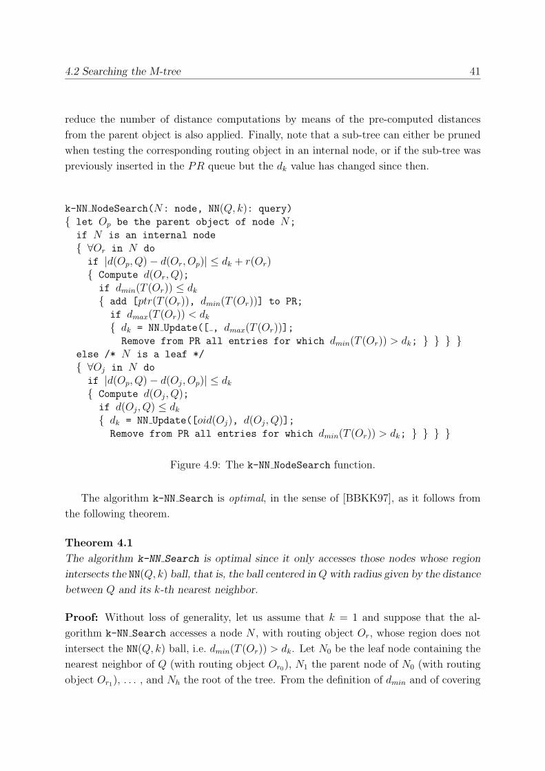
4.2 Searching the M-tree 41
reduce the number of distance computations by means of the pre-computed distances
from the parent object is also applied. Finally, note that a sub-tree can either be pruned
when testing the corresponding routing object in an internal node, or if the sub-tree was
previously inserted in the PR queue but the dk value has changed since then.
k-NN NodeSearch(N: node, NN(Q, k): query)
{ let Op be the parent object of node N;
if N is an internal node
{ ∀Or in N do
if |d(Op, Q)− d(Or, Op)| ≤ dk + r(Or){ Compute d(Or, Q);if dmin(T (Or)) ≤ dk{ add [ptr(T (Or)), dmin(T (Or))] to PR;
if dmax(T (Or)) < dk{ dk = NN Update([ , dmax(T (Or))];Remove from PR all entries for which dmin(T (Or)) > dk; } } } }
else /* N is a leaf */
{ ∀Oj in N do
if |d(Op, Q)− d(Oj, Op)| ≤ dk{ Compute d(Oj, Q);if d(Oj, Q) ≤ dk{ dk = NN Update([oid(Oj), d(Oj, Q)];Remove from PR all entries for which dmin(T (Or)) > dk; } } } }
Figure 4.9: The k-NN NodeSearch function.
The algorithm k-NN Search is optimal, in the sense of [BBKK97], as it follows from
the following theorem.
Theorem 4.1
The algorithm k-NN Search is optimal since it only accesses those nodes whose region
intersects the NN(Q, k) ball, that is, the ball centered inQ with radius given by the distance
between Q and its k-th nearest neighbor.
Proof: Without loss of generality, let us assume that k = 1 and suppose that the al-
gorithm k-NN Search accesses a node N , with routing object Or, whose region does not
intersect the NN(Q, k) ball, i.e. dmin(T (Or)) > dk. Let N0 be the leaf node containing the
nearest neighbor of Q (with routing object Or0), N1 the parent node of N0 (with routing
object Or1), . . . , and Nh the root of the tree. From the definition of dmin and of covering
42 Chapter 4. The M-tree
radius, it follows that
dk ≥ dmin(T (Or0)) ≥ . . . ≥ dmin(T (Orh−1))
Thus, it is
dmin(T (Or)) > dk ≥ dmin(T (Or0)) ≥ . . . ≥ dmin(T (Orh−1))
During the search process, the root node Nh is replaced in the PR queue by its children
Nh−1, and so on, until the leaf node N0 is loaded. Since dmin(T (Or)) > dmin(T (Or0)),
N cannot be accessed until N0 has been loaded. If N0 is loaded, however, all the nodes
having dmin greater than dk are removed form the PR queue. Hence, N is not accessed
and this contradicts the assumption. ✷
4.3 How M-tree Grows
In general, algorithms for building the M-tree have to specify the way how objects are
inserted and deleted, and how node overflows and underflows are managed.
The Insert algorithm recursively descends the M-tree to locate the most suitable leaf
node for accommodating the new object, On. If insertion into the chosen node causes
overflow, a split is triggered and updates are propagated up to higher level(s) of the tree.
The basic rationale used to find the “most suitable” leaf node is to follow a path which
would avoid any enlargement of the covering radius, i.e. at each level of the tree, a sub-tree
T (Or) is chosen, for which it is d(Or, On) ≤ r(Or). If multiple paths with this property
exist, the one for which object On is closest to the routing object, that is, d(Or, On) is
minimum, is chosen. Intuitively, this heuristics tries to obtain well-clustered sub-trees,
which has a beneficial effect on performance.
If no routing object for which d(Or, On) ≤ r(Or) exists, enlargement of a covering
radius is indispensable. In this case, the choice is to minimize the increase of the covering
radius, that is the quantity d(Or, On)−r(Or). This choice is tightly related to the heuristic
criterion that suggests to minimize the overall “volume” covered by routing objects in the
current node. The Insert algorithm is given in Figure 4.10.
The pruning technique of Lemma 4.2 can be applied in the Insert algorithm to reduce
the number of computed distance by using stored and precomputed distances. Let O∗i
be the optimal choice obtained so far: In each entry entry(Oi) of N we have stored the
distance d(Op, Oi), and, at the previous stage of the Insert algorithm, we have computed
the distance d(On, Op), where Op is the parent object of Oi. The value |d(On, Op) −d(Op, Oi)| is, therefore, a lower bound on d(On, Oi), as follows from triangle inequality. If
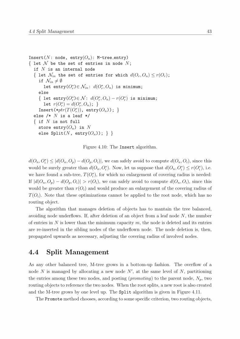
4.4 Split Management 43
Insert(N: node, entry(On): M-tree entry)
{ let N be the set of entries in node N;
if N is an internal node
{ let Nin the set of entries for which d(Or, On) ≤ r(Or);if Nin = ∅let entry(O∗
r)∈ Nin: d(O∗r , On) is minimum;
else
{ let entry(O∗r)∈ N: d(O∗
r , On)− r(O∗r) is minimum;
let r(O∗r) = d(O∗
r , On); }Insert(*ptr(T (O∗
r)), entry(On)); }else /* N is a leaf */
{ if N is not full
store entry(On) in Nelse Split(N, entry(On)); } }
Figure 4.10: The Insert algorithm.
d(On, O∗i ) ≤ |d(On, Op)− d(Op, Oi)|, we can safely avoid to compute d(On, Oi), since this
would be surely greater than d(On, O∗i ). Now, let us suppose that d(On, O
∗i ) ≤ r(O∗
i ), i.e.
we have found a sub-tree, T (O∗i ), for which no enlargement of covering radius is needed:
If |d(On, Op) − d(Op, Oi)| > r(Oi), we can safely avoid to compute d(On, Oi), since this
would be greater than r(Oi) and would produce an enlargement of the covering radius of
T (Oi). Note that these optimizations cannot be applied to the root node, which has no
routing object.
The algorithm that manages deletion of objects has to mantain the tree balanced,
avoiding node underflows. If, after deletion of an object from a leaf node N , the number
of entries in N is lower than the minimum capacity m, the node is deleted and its entries
are re-inserted in the sibling nodes of the underflown node. The node deletion is, then,
propagated upwards as necessary, adjusting the covering radius of involved nodes.
4.4 Split Management
As any other balanced tree, M-tree grows in a bottom-up fashion. The overflow of a
node N is managed by allocating a new node N ′, at the same level of N , partitioningthe entries among these two nodes, and posting (promoting) to the parent node, Np, two
routing objects to reference the two nodes. When the root splits, a new root is also created
and the M-tree grows by one level up. The Split algorithm is given in Figure 4.11.
The Promotemethod chooses, according to some specific criterion, two routing objects,
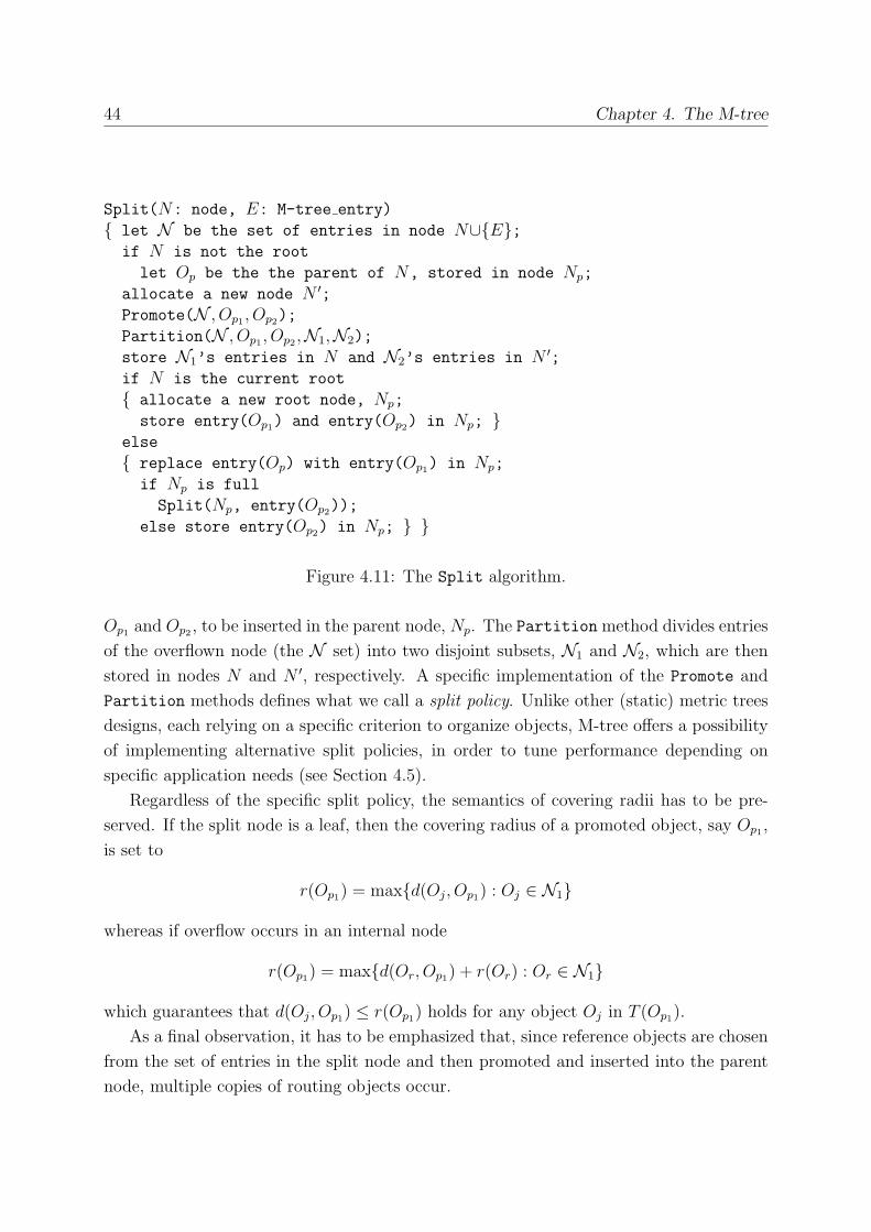
44 Chapter 4. The M-tree
Split(N: node, E: M-tree entry)
{ let N be the set of entries in node N∪{E};if N is not the root
let Op be the the parent of N, stored in node Np;
allocate a new node N ′;Promote(N , Op1, Op2);
Partition(N , Op1, Op2 ,N1,N2);
store N1’s entries in N and N2’s entries in N ′;if N is the current root
{ allocate a new root node, Np;
store entry(Op1) and entry(Op2) in Np; }else
{ replace entry(Op) with entry(Op1) in Np;
if Np is full
Split(Np, entry(Op2));
else store entry(Op2) in Np; } }
Figure 4.11: The Split algorithm.
Op1 and Op2 , to be inserted in the parent node, Np. The Partitionmethod divides entries
of the overflown node (the N set) into two disjoint subsets, N1 and N2, which are then
stored in nodes N and N ′, respectively. A specific implementation of the Promote and
Partition methods defines what we call a split policy. Unlike other (static) metric trees
designs, each relying on a specific criterion to organize objects, M-tree offers a possibility
of implementing alternative split policies, in order to tune performance depending on
specific application needs (see Section 4.5).
Regardless of the specific split policy, the semantics of covering radii has to be pre-
served. If the split node is a leaf, then the covering radius of a promoted object, say Op1 ,
is set to
r(Op1) = max{d(Oj, Op1) : Oj ∈ N1}
whereas if overflow occurs in an internal node
r(Op1) = max{d(Or, Op1) + r(Or) : Or ∈ N1}
which guarantees that d(Oj, Op1) ≤ r(Op1) holds for any object Oj in T (Op1).
As a final observation, it has to be emphasized that, since reference objects are chosen
from the set of entries in the split node and then promoted and inserted into the parent
node, multiple copies of routing objects occur.
4.5 Split Policies 45
4.5 Split Policies
Effective implementation of M-tree requires a careful choice of specific algorithms for
managing the tree evolution. In particular, split operations should try to satisfy a set of
somewhat contrasting requirements, which can be summarized as follows:
Minimum “volume”. Since pruning of the search space is tightly related to the “vol-
umes” covered by routing objects, and these are directly related to the values of the
covering radii, it is advisable to keep such values as small as possible.
Minimum “overlap”. In order to reduce the number of paths that have to be traversed
for answering a query, it would be convenient to have a tree organization such
that the regions covered by the routing objects are well-separated. It has to be
remarked that, in a generic metric space, minimization of overlap has no precise
mathematical formulation. In other terms, given two non-disjoint regions, it is not
possible, without a detailed knowledge of the distance function, to quantify the
amount of overlap. However, when applying this heuristics to the split algorithm,
from a qualitative point of view, it can be said that, for fixed values of the covering
radii, the distance between the two chosen reference objects should be maximized.
Balanced split. This is a classical requirement for height-balanced access methods,
which also aims to keep the height of the tree as small as possible.
Although the above requirements can be considered quite “standard” also for SAMs
[BKSS90], in the “metric space” scenario they have to be considered from a rather different
perspective. Besides the already done observations related to the overlap definition, at
least two additional facts are still to be noticed:
1. The possible high CPU cost of computing distances suggests for choosing reference
objects also algorithms which would otherwise be considered naıve (e.g. a random
choice) — a quadratic cost split algorithm may turn to be unacceptable in many
cases.
2. Balanced distribution of entries (possibly specified by a minimum threshold value)
does not appear to be a really pressing requirement, compared to the other two.
While satisfying this criterion with multi-dimensional access methods can usually
be accomplished by enlarging regions along only the necessary dimensions, in a
metric space the consequent increase of the covering radius would propagate to all
the “dimensions”.

46 Chapter 4. The M-tree
Since it seems quite difficult to rely on well-founded arguments to a priori rule out
some partitioning heuristic criteria, we decided to start with a moderately large set of
alternative solutions, and to experimentally evaluate all of them (see Section 4.7).
4.5.1 Choosing the Routing Objects
The Promote method determines, given a set of entries, N , two objects to be promotedand stored into the parent node. The specific algorithms we consider can first be classified
according to whether or not they “confirm” the original routing object in its role.
Definition 4.1 (Confirmed split policy)
A confirmed split policy chooses as one of the promoted objects, say Op1 , the object Op,
i.e. the routing object of the split node.
In other terms, a confirmed split policy just “extracts” a region, centered on the second
routing object, Op2 , from the region which will still remain centered on Op. In general,
this simplifies split execution and reduces the number of distance computations.
We implemented and experimentally evaluated (see Section 4.7) all of the following
alternatives, both in the confirmed and in the non-confirmed version.
RANDOM This variant simply selects in a random way the reference objects. Although it
is not a “smart” strategy, it is fast and its performance can be used as a reference
for other policies.
SAMPLING This is the RANDOM policy, but iterated over a sample of objects of size s > 1.
For each of the s(s− 1)/2 pairs of objects in the sample, entries are distributed andpotential covering radii established. The pair for which the resulting maximum of
covering radii is minimum is then selected. In case of confirmed promotion, only s
different distributions are tried. The sample size in our experiments was 1/10-th of
the node capacity, unless otherwise stated.
M LB DIST The acronym stands for “Maximum Lower Bound on DISTance”. This policy
differs from previous ones in that it only uses precomputed stored distances. In the
confirmed version, where Op1 ≡ Op, the algorithm determines Op2 as the farthest
object from Op, that is
d(Op2 , Op) = maxj{d(Oj, Op)}
M UB DIST The acronym stands for “Maximum Upper Bound on DISTance”. This variant
is the pessimistic version of M LB DIST, and has the purpose of maximizing the upper
4.5 Split Policies 47
bound of the distance of the objects to be promoted. This is achieved by selecting
the two objects which are farthest from Op, that is
d(Op1 , Op) = maxj{d(Oj, Op)}
d(Op2 , Op) = maxj{d(Oj, Op), Oj = Op1}
mM LB RAD This variant is basically conceived for confirmed promotion, and can be con-
cisely explained as follows. Consider the pair-wise lower bounds on distances among
all the entries in the node (no new actual distance has to be computed for this pur-
pose). For each object Oi compute maxj{|d(Oi, Op)− d(Oj, Op)|} and promote theobject for which the maximum is minimized. The acronym, hence, stands for “min-
imum Maximum Lower Bound on RADius”. This criterion selects for promotion
object Op2 which has an “intermediate” distance from Op.
mM UB RAD This variant is the “pessimistic” version of mM LB RAD, in that it uses upper
bounds d(Oi, Op) + d(Oj, Op). The net effect is to promote an object which is the
closest to Op1 .
mM AVG RAD This is a variant which tries to be “neutral” with respect to lower and upper
bound information, taking their average and then applying the min-Max selection
criterion.
m RAD The “minimum (sum of) RADii” algorithm is the most complex in terms of distance
computations. It considers all possible pairs of objects and, after partitioning the
set of entries, promotes the pair of objects for which the sum of covering radii,
r(Op1) + r(Op2), is minimum.
mM RAD This is similar to m RAD, but it minimizes the maximum of the two radii.
Figure 4.12 provides a graphical intuition on the behavior of some of the split variants.
4.5.2 Distribution of the Entries
Given a set of entries N and two routing objects Op1 and Op2 , the problem is how to
efficiently partitionN into two subsets, N1 andN2. For this purpose we consider two basic
strategies. The first one is based on the idea of the generalized hyperplane decomposition
[Uhl91] and leads to unbalanced splits, whereas the second obtains a balanced distribution.
They can be shortly described as follows.
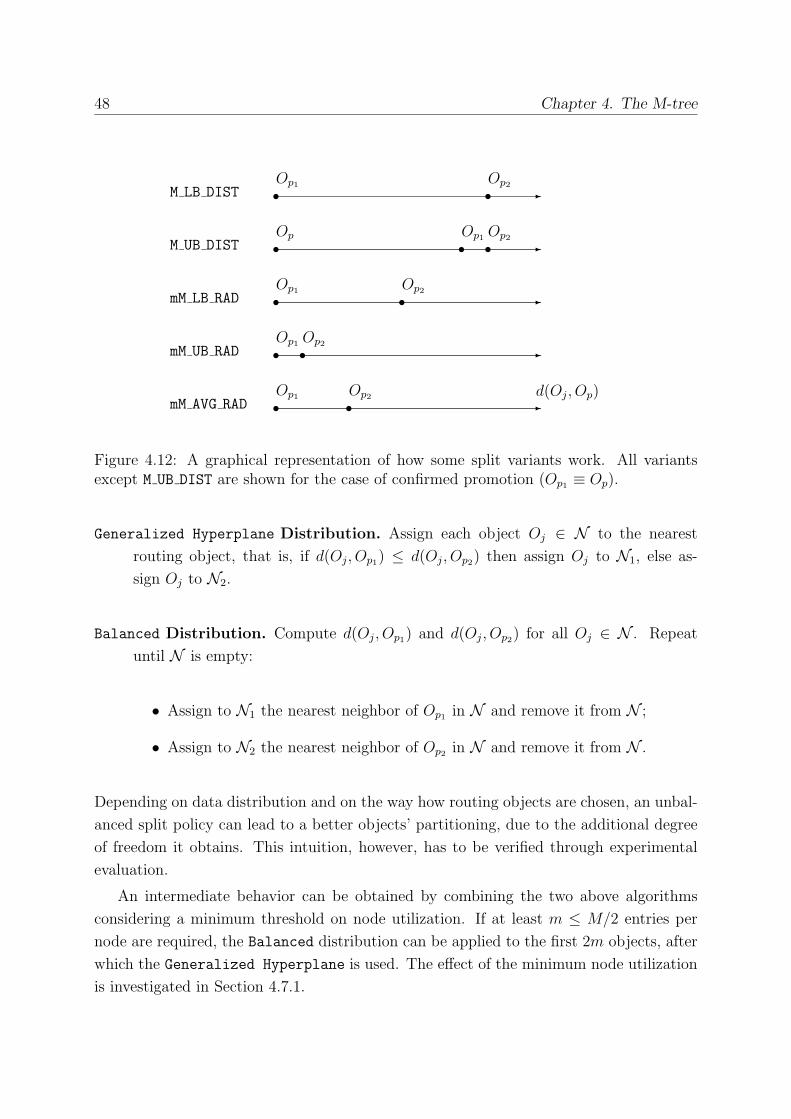
48 Chapter 4. The M-tree
✲Op1
✲Op1
✲Op1
✲Op1
✲Op1
M LB DIST
M UB DIST
mM LB RAD
mM UB RAD
mM AVG RAD
Op2
�
�
�
�
�
Op2
�
Op2
Op
�
�
�
Op2
� �
Op2 d(Oj, Op)
Figure 4.12: A graphical representation of how some split variants work. All variantsexcept M UB DIST are shown for the case of confirmed promotion (Op1 ≡ Op).
Generalized Hyperplane Distribution. Assign each object Oj ∈ N to the nearest
routing object, that is, if d(Oj, Op1) ≤ d(Oj, Op2) then assign Oj to N1, else as-
sign Oj to N2.
Balanced Distribution. Compute d(Oj, Op1) and d(Oj, Op2) for all Oj ∈ N . Repeatuntil N is empty:
• Assign to N1 the nearest neighbor of Op1 in N and remove it from N ;
• Assign to N2 the nearest neighbor of Op2 in N and remove it from N .
Depending on data distribution and on the way how routing objects are chosen, an unbal-
anced split policy can lead to a better objects’ partitioning, due to the additional degree
of freedom it obtains. This intuition, however, has to be verified through experimental
evaluation.
An intermediate behavior can be obtained by combining the two above algorithms
considering a minimum threshold on node utilization. If at least m ≤ M/2 entries per
node are required, the Balanced distribution can be applied to the first 2m objects, after
which the Generalized Hyperplane is used. The effect of the minimum node utilization
is investigated in Section 4.7.1.
4.6 Implementation Issues 49
4.6 Implementation Issues
Our M-tree implementation is based on the Generalized Search Tree (GiST) C++ package,
a structure extendible both in the data types and in the queries it can support [HNP95].4
A GiST is a balanced tree with variable fanout k, where m < k < M (m and M being
the minimum and the maximum node capacity, respectively). Leaf nodes store entries
having the form E = (p, ptr), where p is a predicate used as a search key and ptr is the
object identifier. Internal nodes store entries having the form E = (p, ptr), where p is a
predicate used as a search key and ptr is the pointer to another tree node. By using “key
compression” techniques, a given predicate p may take as little as zero bytes of storage,
as for B-trees. In this framework, a specific access method is specified by defining the
predicate p for each entry and by providing the code for a limited set of required methods:
Consistent(E, q). Given an entry E = (p, ptr), and a query q, returns false iff p∧ q canbe guaranteed unsatisfiable, and true otherwise.
Union(P ). Given a set P of entries {(p1, ptr1), . . . , (pn, ptrn)}, returns some predicate rthat holds for all objects stored below ptr1 through ptrn.
Penalty(E1, E2). Given two entries E1 = (p1, ptr1) and E2 = (p2, ptr2), returns a
domain-specific penalty for inserting E2 into the sub-tree rooted at E1.
PickSplit(P ). Given a set P of M + 1 entries, splits P into two sets of entries P1 and
P2, each of size at least m.
For the M-tree, the predicate associated to each entry of the tree consists of the entry
region, that is the pair (Or, r(Or)), where r(Or) = 0 for ground entries, i.e. for entries
in leaf nodes. The basic M-tree version of Consistent, thus, returns false iff the region
associated with the entry E = ((Oj, r(Oj)), ptrj) is guaranteed to be outside of the query
region, i.e. iff d(Oj, Q) > r(Oj)+rQ. The search algorithm RS, then, uses this information
to descend all paths in the tree whose entries are consistent with the query. Consistent
can also be used for k-nearest neighbor query, by assigning to the query radius rQ the
actual distance to the k-th nearest neighbor obtained so far, i.e. dk.
The Union method is used in the insertion phase to compute the covering radius for a
node N , given the set P of entries stored within N . Of course, this can be computed as:
r(Or) = max{d(Or, Oj) + r(Oj) : E = ((Oj, r(Oj)), ptrj) ∈ P}4The GiST source code is freely available at URL http://gist.cs.berkeley.edu:8000/gist/.
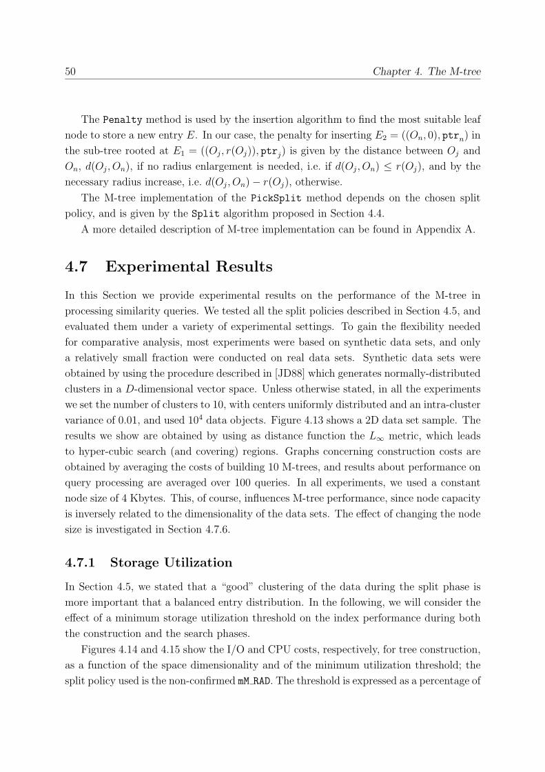
50 Chapter 4. The M-tree
The Penalty method is used by the insertion algorithm to find the most suitable leaf
node to store a new entry E. In our case, the penalty for inserting E2 = ((On, 0), ptrn) in
the sub-tree rooted at E1 = ((Oj, r(Oj)), ptrj) is given by the distance between Oj and
On, d(Oj, On), if no radius enlargement is needed, i.e. if d(Oj, On) ≤ r(Oj), and by the
necessary radius increase, i.e. d(Oj, On)− r(Oj), otherwise.
The M-tree implementation of the PickSplit method depends on the chosen split
policy, and is given by the Split algorithm proposed in Section 4.4.
A more detailed description of M-tree implementation can be found in Appendix A.
4.7 Experimental Results
In this Section we provide experimental results on the performance of the M-tree in
processing similarity queries. We tested all the split policies described in Section 4.5, and
evaluated them under a variety of experimental settings. To gain the flexibility needed
for comparative analysis, most experiments were based on synthetic data sets, and only
a relatively small fraction were conducted on real data sets. Synthetic data sets were
obtained by using the procedure described in [JD88] which generates normally-distributed
clusters in a D-dimensional vector space. Unless otherwise stated, in all the experiments
we set the number of clusters to 10, with centers uniformly distributed and an intra-cluster
variance of 0.01, and used 104 data objects. Figure 4.13 shows a 2D data set sample. The
results we show are obtained by using as distance function the L∞ metric, which leads
to hyper-cubic search (and covering) regions. Graphs concerning construction costs are
obtained by averaging the costs of building 10 M-trees, and results about performance on
query processing are averaged over 100 queries. In all experiments, we used a constant
node size of 4 Kbytes. This, of course, influences M-tree performance, since node capacity
is inversely related to the dimensionality of the data sets. The effect of changing the node
size is investigated in Section 4.7.6.
4.7.1 Storage Utilization
In Section 4.5, we stated that a “good” clustering of the data during the split phase is
more important that a balanced entry distribution. In the following, we will consider the
effect of a minimum storage utilization threshold on the index performance during both
the construction and the search phases.
Figures 4.14 and 4.15 show the I/O and CPU costs, respectively, for tree construction,
as a function of the space dimensionality and of the minimum utilization threshold; the
split policy used is the non-confirmed mM RAD. The threshold is expressed as a percentage of
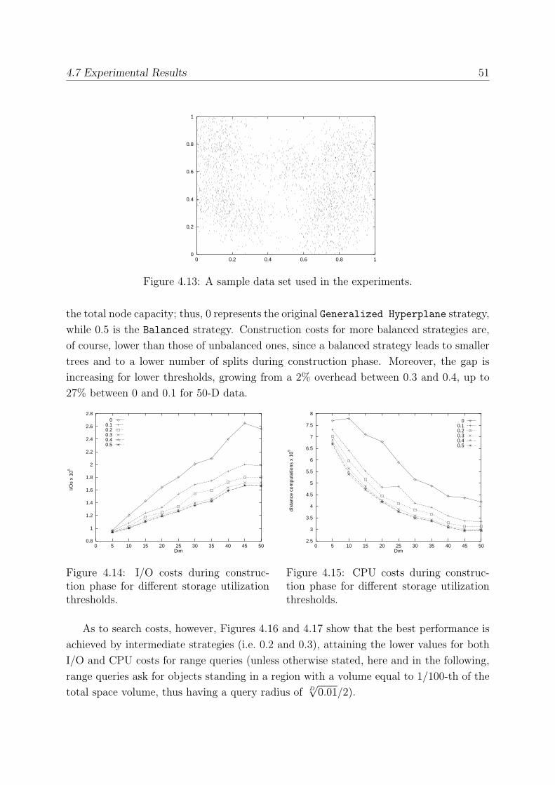
4.7 Experimental Results 51
0
0.2
0.4
0.6
0.8
1
0 0.2 0.4 0.6 0.8 1
Figure 4.13: A sample data set used in the experiments.
the total node capacity; thus, 0 represents the original Generalized Hyperplane strategy,
while 0.5 is the Balanced strategy. Construction costs for more balanced strategies are,
of course, lower than those of unbalanced ones, since a balanced strategy leads to smaller
trees and to a lower number of splits during construction phase. Moreover, the gap is
increasing for lower thresholds, growing from a 2% overhead between 0.3 and 0.4, up to
27% between 0 and 0.1 for 50-D data.
0.8
1
1.2
1.4
1.6
1.8
2
2.2
2.4
2.6
2.8
0 5 10 15 20 25 30 35 40 45 50
I/Os
x 10
5
Dim
00.10.20.30.40.5
Figure 4.14: I/O costs during construc-tion phase for different storage utilizationthresholds.
2.5
3
3.5
4
4.5
5
5.5
6
6.5
7
7.5
8
0 5 10 15 20 25 30 35 40 45 50
dist
ance
com
puta
tions
x 1
05
Dim
00.10.20.30.40.5
Figure 4.15: CPU costs during construc-tion phase for different storage utilizationthresholds.
As to search costs, however, Figures 4.16 and 4.17 show that the best performance is
achieved by intermediate strategies (i.e. 0.2 and 0.3), attaining the lower values for both
I/O and CPU costs for range queries (unless otherwise stated, here and in the following,
range queries ask for objects standing in a region with a volume equal to 1/100-th of the
total space volume, thus having a query radius of D√0.01/2).
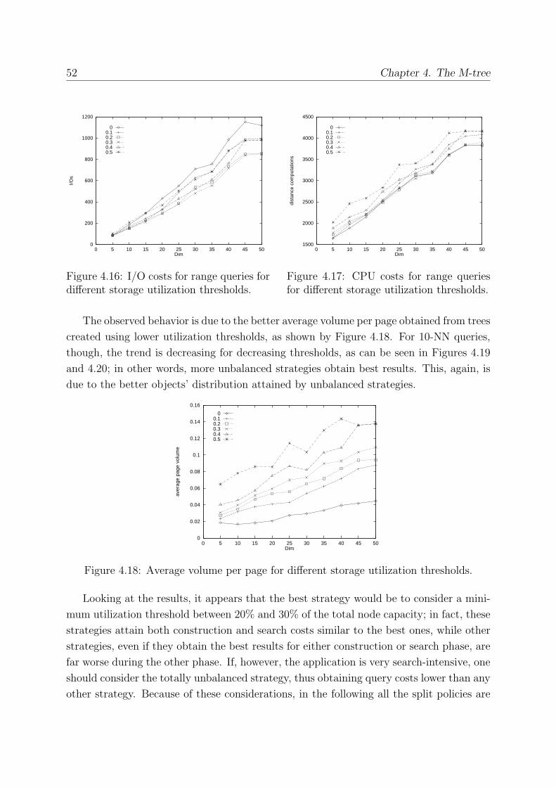
52 Chapter 4. The M-tree
0
200
400
600
800
1000
1200
0 5 10 15 20 25 30 35 40 45 50
I/Os
Dim
00.10.20.30.40.5
Figure 4.16: I/O costs for range queries fordifferent storage utilization thresholds.
1500
2000
2500
3000
3500
4000
4500
0 5 10 15 20 25 30 35 40 45 50
dist
ance
com
puta
tions
Dim
00.10.20.30.40.5
Figure 4.17: CPU costs for range queriesfor different storage utilization thresholds.
The observed behavior is due to the better average volume per page obtained from trees
created using lower utilization thresholds, as shown by Figure 4.18. For 10-NN queries,
though, the trend is decreasing for decreasing thresholds, as can be seen in Figures 4.19
and 4.20; in other words, more unbalanced strategies obtain best results. This, again, is
due to the better objects’ distribution attained by unbalanced strategies.
0
0.02
0.04
0.06
0.08
0.1
0.12
0.14
0.16
0 5 10 15 20 25 30 35 40 45 50
aver
age
page
vol
ume
Dim
00.10.20.30.40.5
Figure 4.18: Average volume per page for different storage utilization thresholds.
Looking at the results, it appears that the best strategy would be to consider a mini-
mum utilization threshold between 20% and 30% of the total node capacity; in fact, these
strategies attain both construction and search costs similar to the best ones, while other
strategies, even if they obtain the best results for either construction or search phase, are
far worse during the other phase. If, however, the application is very search-intensive, one
should consider the totally unbalanced strategy, thus obtaining query costs lower than any
other strategy. Because of these considerations, in the following all the split policies are
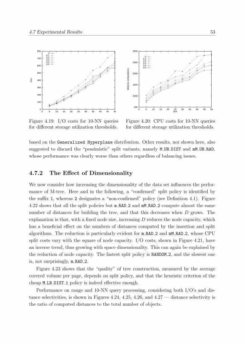
4.7 Experimental Results 53
0
100
200
300
400
500
600
700
800
0 5 10 15 20 25 30 35 40 45 50
I/Os
00.10.20.30.40.5
Figure 4.19: I/O costs for 10-NN queriesfor different storage utilization thresholds.
500
1000
1500
2000
2500
3000
0 5 10 15 20 25 30 35 40 45 50
dist
ance
com
puta
tions
Dim
00.10.20.30.40.5
Figure 4.20: CPU costs for 10-NN queriesfor different storage utilization thresholds.
based on the Generalized Hyperplane distribution. Other results, not shown here, also
suggested to discard the “pessimistic” split variants, namely M UB DIST and mM UB RAD,
whose performance was clearly worse than others regardless of balancing issues.
4.7.2 The Effect of Dimensionality
We now consider how increasing the dimensionality of the data set influences the perfor-
mance of M-tree. Here and in the following, a “confirmed” split policy is identified by
the suffix 1, whereas 2 designates a “non-confirmed” policy (see Definition 4.1). Figure
4.22 shows that all the split policies but m RAD 2 and mM RAD 2 compute almost the same
number of distances for building the tree, and that this decreases when D grows. The
explanation is that, with a fixed node size, increasing D reduces the node capacity, which
has a beneficial effect on the numbers of distances computed by the insertion and split
algorithms. The reduction is particularly evident for m RAD 2 and mM RAD 2, whose CPU
split costs vary with the square of node capacity. I/O costs, shown in Figure 4.21, have
an inverse trend, thus growing with space dimensionality. This can again be explained by
the reduction of node capacity. The fastest split policy is RANDOM 2, and the slowest one
is, not surprisingly, m RAD 2.
Figure 4.23 shows that the “quality” of tree construction, measured by the average
covered volume per page, depends on split policy, and that the heuristic criterion of the
cheap M LB DIST 1 policy is indeed effective enough.
Performance on range and 10-NN query processing, considering both I/O’s and dis-
tance selectivities, is shown in Figures 4.24, 4.25, 4.26, and 4.27 — distance selectivity is
the ratio of computed distances to the total number of objects.
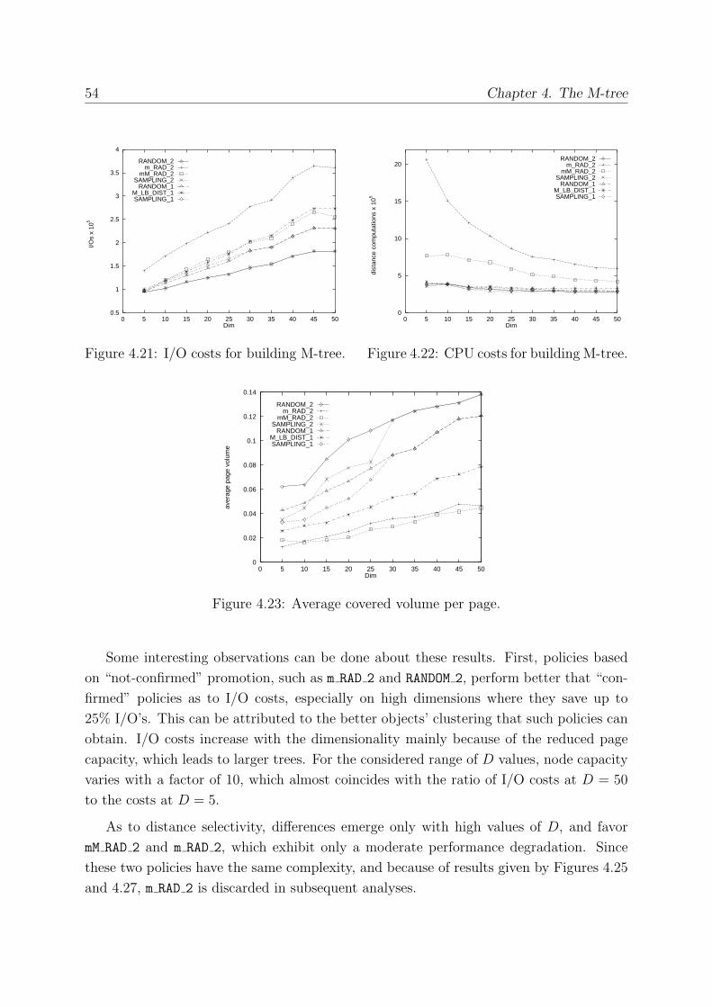
54 Chapter 4. The M-tree
0.5
1
1.5
2
2.5
3
3.5
4
0 5 10 15 20 25 30 35 40 45 50
I/Os
x 10
5
Dim
RANDOM_2m_RAD_2
mM_RAD_2SAMPLING_2
RANDOM_1M_LB_DIST_1SAMPLING_1
Figure 4.21: I/O costs for building M-tree.
0
5
10
15
20
0 5 10 15 20 25 30 35 40 45 50
dist
ance
com
puta
tions
x 1
05
Dim
RANDOM_2m_RAD_2
mM_RAD_2SAMPLING_2
RANDOM_1M_LB_DIST_1SAMPLING_1
Figure 4.22: CPU costs for building M-tree.
0
0.02
0.04
0.06
0.08
0.1
0.12
0.14
0 5 10 15 20 25 30 35 40 45 50
aver
age
page
vol
ume
Dim
RANDOM_2m_RAD_2
mM_RAD_2SAMPLING_2
RANDOM_1M_LB_DIST_1SAMPLING_1
Figure 4.23: Average covered volume per page.
Some interesting observations can be done about these results. First, policies based
on “not-confirmed” promotion, such as m RAD 2 and RANDOM 2, perform better that “con-
firmed” policies as to I/O costs, especially on high dimensions where they save up to
25% I/O’s. This can be attributed to the better objects’ clustering that such policies can
obtain. I/O costs increase with the dimensionality mainly because of the reduced page
capacity, which leads to larger trees. For the considered range of D values, node capacity
varies with a factor of 10, which almost coincides with the ratio of I/O costs at D = 50
to the costs at D = 5.
As to distance selectivity, differences emerge only with high values of D, and favor
mM RAD 2 and m RAD 2, which exhibit only a moderate performance degradation. Since
these two policies have the same complexity, and because of results given by Figures 4.25
and 4.27, m RAD 2 is discarded in subsequent analyses.
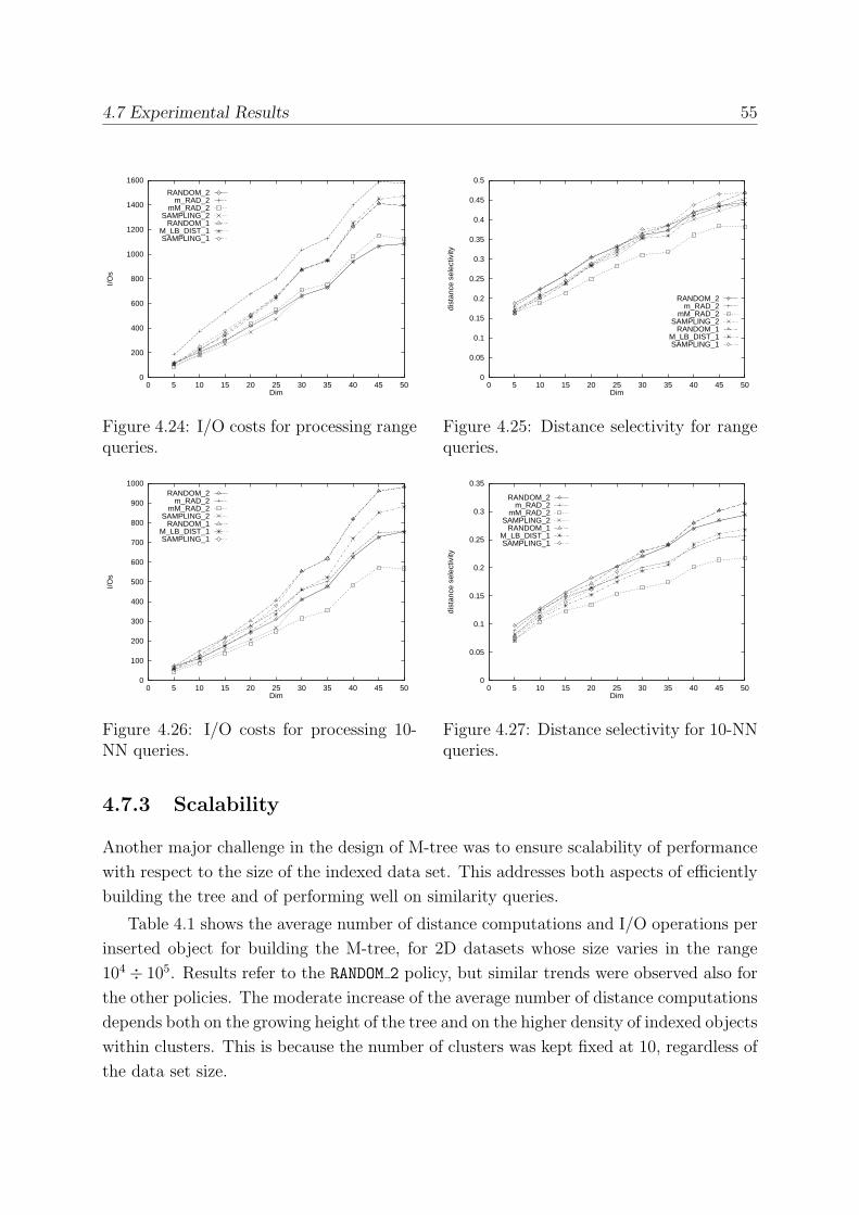
4.7 Experimental Results 55
0
200
400
600
800
1000
1200
1400
1600
0 5 10 15 20 25 30 35 40 45 50
I/Os
Dim
RANDOM_2m_RAD_2
mM_RAD_2SAMPLING_2
RANDOM_1M_LB_DIST_1SAMPLING_1
Figure 4.24: I/O costs for processing rangequeries.
0
0.05
0.1
0.15
0.2
0.25
0.3
0.35
0.4
0.45
0.5
0 5 10 15 20 25 30 35 40 45 50
dist
ance
sel
ectiv
ity
Dim
RANDOM_2m_RAD_2
mM_RAD_2SAMPLING_2
RANDOM_1M_LB_DIST_1SAMPLING_1
Figure 4.25: Distance selectivity for rangequeries.
0
100
200
300
400
500
600
700
800
900
1000
0 5 10 15 20 25 30 35 40 45 50
I/Os
Dim
RANDOM_2m_RAD_2
mM_RAD_2SAMPLING_2
RANDOM_1M_LB_DIST_1SAMPLING_1
Figure 4.26: I/O costs for processing 10-NN queries.
0
0.05
0.1
0.15
0.2
0.25
0.3
0.35
0 5 10 15 20 25 30 35 40 45 50
dist
ance
sel
ectiv
ity
Dim
RANDOM_2m_RAD_2
mM_RAD_2SAMPLING_2
RANDOM_1M_LB_DIST_1SAMPLING_1
Figure 4.27: Distance selectivity for 10-NNqueries.
4.7.3 Scalability
Another major challenge in the design of M-tree was to ensure scalability of performance
with respect to the size of the indexed data set. This addresses both aspects of efficiently
building the tree and of performing well on similarity queries.
Table 4.1 shows the average number of distance computations and I/O operations per
inserted object for building the M-tree, for 2D datasets whose size varies in the range
104 ÷ 105. Results refer to the RANDOM 2 policy, but similar trends were observed also for
the other policies. The moderate increase of the average number of distance computations
depends both on the growing height of the tree and on the higher density of indexed objects
within clusters. This is because the number of clusters was kept fixed at 10, regardless of
the data set size.
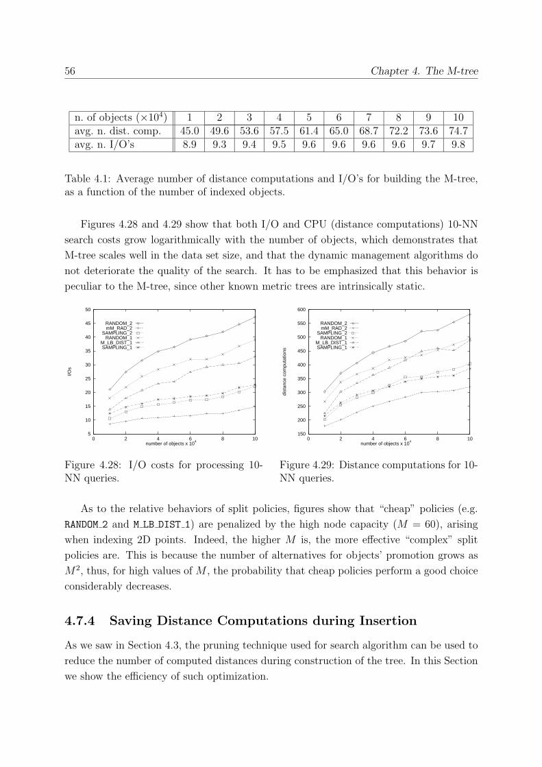
56 Chapter 4. The M-tree
n. of objects (×104) 1 2 3 4 5 6 7 8 9 10avg. n. dist. comp. 45.0 49.6 53.6 57.5 61.4 65.0 68.7 72.2 73.6 74.7avg. n. I/O’s 8.9 9.3 9.4 9.5 9.6 9.6 9.6 9.6 9.7 9.8
Table 4.1: Average number of distance computations and I/O’s for building the M-tree,as a function of the number of indexed objects.
Figures 4.28 and 4.29 show that both I/O and CPU (distance computations) 10-NN
search costs grow logarithmically with the number of objects, which demonstrates that
M-tree scales well in the data set size, and that the dynamic management algorithms do
not deteriorate the quality of the search. It has to be emphasized that this behavior is
peculiar to the M-tree, since other known metric trees are intrinsically static.
5
10
15
20
25
30
35
40
45
50
0 2 4 6 8 10
I/Os
number of objects x 104
RANDOM_2mM_RAD_2
SAMPLING_2RANDOM_1
M_LB_DIST_1SAMPLING_1
Figure 4.28: I/O costs for processing 10-NN queries.
150
200
250
300
350
400
450
500
550
600
0 2 4 6 8 10
dist
ance
com
puta
tions
number of objects x 104
RANDOM_2mM_RAD_2
SAMPLING_2RANDOM_1
M_LB_DIST_1SAMPLING_1
Figure 4.29: Distance computations for 10-NN queries.
As to the relative behaviors of split policies, figures show that “cheap” policies (e.g.
RANDOM 2 and M LB DIST 1) are penalized by the high node capacity (M = 60), arising
when indexing 2D points. Indeed, the higher M is, the more effective “complex” split
policies are. This is because the number of alternatives for objects’ promotion grows as
M2, thus, for high values of M , the probability that cheap policies perform a good choice
considerably decreases.
4.7.4 Saving Distance Computations during Insertion
As we saw in Section 4.3, the pruning technique used for search algorithm can be used to
reduce the number of computed distances during construction of the tree. In this Section
we show the efficiency of such optimization.
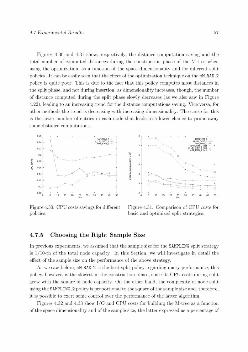
4.7 Experimental Results 57
Figures 4.30 and 4.31 show, respectively, the distance computation saving and the
total number of computed distances during the construction phase of the M-tree when
using the optimization, as a function of the space dimensionality and for different split
policies. It can be easily seen that the effect of the optimization technique on the mM RAD 2
policy is quite poor: This is due to the fact that this policy computes most distances in
the split phase, and not during insertion; as dimensionality increases, though, the number
of distance computed during the split phase slowly decreases (as we also saw in Figure
4.22), leading to an increasing trend for the distance computations saving. Vice versa, for
other methods the trend is decreasing with increasing dimensionality: The cause for this
is the lower number of entries in each node that leads to a lower chance to prune away
some distance computations.
0.08
0.1
0.12
0.14
0.16
0.18
0.2
0.22
0.24
0.26
0 5 10 15 20 25 30 35 40 45 50
CP
U s
avin
g
Dim
RANDOM_2M_LB_DIST_1
mM_RAD_2
Figure 4.30: CPU costs savings for differentpolicies.
2
3
4
5
6
7
8
0 5 10 15 20 25 30 35 40 45 50
dist
ance
com
puta
tions
x 1
05
Dim
RANDOM_2M_LB_DIST_1
mM_RAD_2RANDOM_2 (opt)
M_LB_DIST_1 (opt)mM_RAD_2 (opt)
Figure 4.31: Comparison of CPU costs forbasic and optimized split strategies.
4.7.5 Choosing the Right Sample Size
In previous experiments, we assumed that the sample size for the SAMPLING split strategy
is 1/10-th of the total node capacity. In this Section, we will investigate in detail the
effect of the sample size on the performance of the above strategy.
As we saw before, mM RAD 2 is the best split policy regarding query performance; this
policy, however, is the slowest in the construction phase, since its CPU costs during split
grow with the square of node capacity. On the other hand, the complexity of node split
using the SAMPLING 2 policy is proportional to the square of the sample size and, therefore,
it is possible to exert some control over the performance of the latter algorithm.
Figures 4.32 and 4.33 show I/O and CPU costs for building the M-tree as a function
of the space dimensionality and of the sample size, the latter expressed as a percentage of
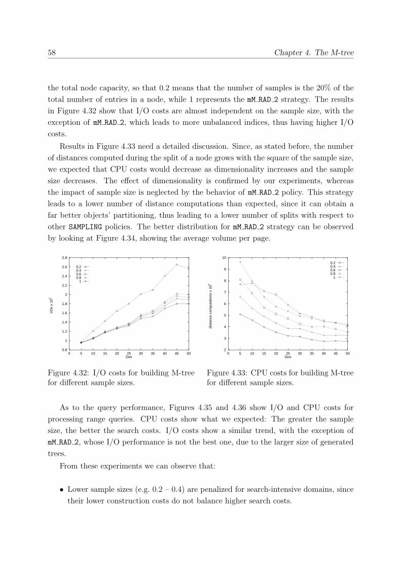
58 Chapter 4. The M-tree
the total node capacity, so that 0.2 means that the number of samples is the 20% of the
total number of entries in a node, while 1 represents the mM RAD 2 strategy. The results
in Figure 4.32 show that I/O costs are almost independent on the sample size, with the
exception of mM RAD 2, which leads to more unbalanced indices, thus having higher I/O
costs.
Results in Figure 4.33 need a detailed discussion. Since, as stated before, the number
of distances computed during the split of a node grows with the square of the sample size,
we expected that CPU costs would decrease as dimensionality increases and the sample
size decreases. The effect of dimensionality is confirmed by our experiments, whereas
the impact of sample size is neglected by the behavior of mM RAD 2 policy. This strategy
leads to a lower number of distance computations than expected, since it can obtain a
far better objects’ partitioning, thus leading to a lower number of splits with respect to
other SAMPLING policies. The better distribution for mM RAD 2 strategy can be observed
by looking at Figure 4.34, showing the average volume per page.
0.8
1
1.2
1.4
1.6
1.8
2
2.2
2.4
2.6
2.8
0 5 10 15 20 25 30 35 40 45 50
I/Os
x 10
5
Dim
0.20.40.60.8
1
Figure 4.32: I/O costs for building M-treefor different sample sizes.
2
3
4
5
6
7
8
9
10
0 5 10 15 20 25 30 35 40 45 50
dist
ance
com
puta
tions
x 1
05
Dim
0.20.40.60.8
1
Figure 4.33: CPU costs for building M-treefor different sample sizes.
As to the query performance, Figures 4.35 and 4.36 show I/O and CPU costs for
processing range queries. CPU costs show what we expected: The greater the sample
size, the better the search costs. I/O costs show a similar trend, with the exception of
mM RAD 2, whose I/O performance is not the best one, due to the larger size of generated
trees.
From these experiments we can observe that:
• Lower sample sizes (e.g. 0.2 – 0.4) are penalized for search-intensive domains, sincetheir lower construction costs do not balance higher search costs.
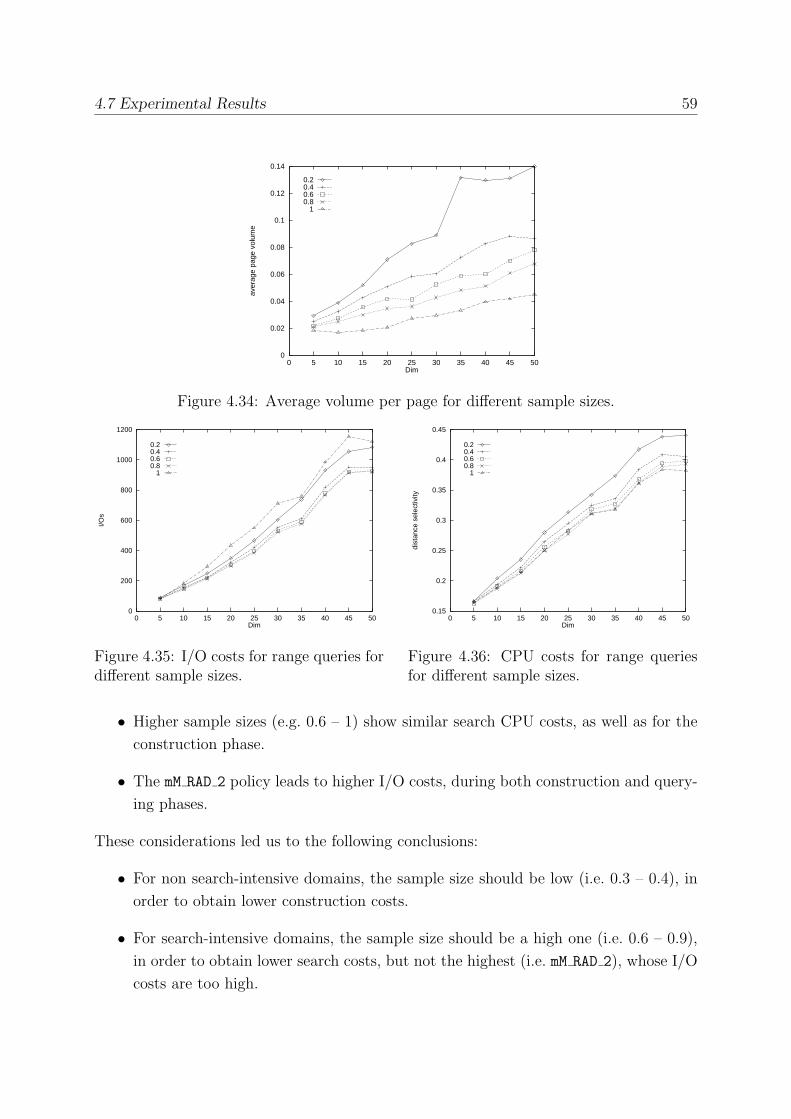
4.7 Experimental Results 59
0
0.02
0.04
0.06
0.08
0.1
0.12
0.14
0 5 10 15 20 25 30 35 40 45 50
aver
age
page
vol
ume
Dim
0.20.40.60.8
1
Figure 4.34: Average volume per page for different sample sizes.
0
200
400
600
800
1000
1200
0 5 10 15 20 25 30 35 40 45 50
I/Os
Dim
0.20.40.60.8
1
Figure 4.35: I/O costs for range queries fordifferent sample sizes.
0.15
0.2
0.25
0.3
0.35
0.4
0.45
0 5 10 15 20 25 30 35 40 45 50
dist
ance
sel
ectiv
ity
Dim
0.20.40.60.8
1
Figure 4.36: CPU costs for range queriesfor different sample sizes.
• Higher sample sizes (e.g. 0.6 – 1) show similar search CPU costs, as well as for theconstruction phase.
• The mM RAD 2 policy leads to higher I/O costs, during both construction and query-
ing phases.
These considerations led us to the following conclusions:
• For non search-intensive domains, the sample size should be low (i.e. 0.3 – 0.4), inorder to obtain lower construction costs.
• For search-intensive domains, the sample size should be a high one (i.e. 0.6 – 0.9),in order to obtain lower search costs, but not the highest (i.e. mM RAD 2), whose I/O
costs are too high.
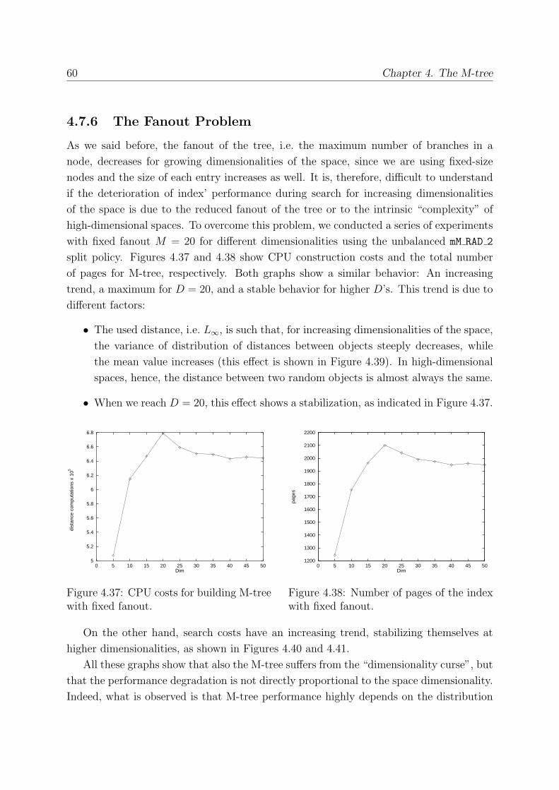
60 Chapter 4. The M-tree
4.7.6 The Fanout Problem
As we said before, the fanout of the tree, i.e. the maximum number of branches in a
node, decreases for growing dimensionalities of the space, since we are using fixed-size
nodes and the size of each entry increases as well. It is, therefore, difficult to understand
if the deterioration of index’ performance during search for increasing dimensionalities
of the space is due to the reduced fanout of the tree or to the intrinsic “complexity” of
high-dimensional spaces. To overcome this problem, we conducted a series of experiments
with fixed fanout M = 20 for different dimensionalities using the unbalanced mM RAD 2
split policy. Figures 4.37 and 4.38 show CPU construction costs and the total number
of pages for M-tree, respectively. Both graphs show a similar behavior: An increasing
trend, a maximum for D = 20, and a stable behavior for higher D’s. This trend is due to
different factors:
• The used distance, i.e. L∞, is such that, for increasing dimensionalities of the space,the variance of distribution of distances between objects steeply decreases, while
the mean value increases (this effect is shown in Figure 4.39). In high-dimensional
spaces, hence, the distance between two random objects is almost always the same.
• When we reach D = 20, this effect shows a stabilization, as indicated in Figure 4.37.
5
5.2
5.4
5.6
5.8
6
6.2
6.4
6.6
6.8
0 5 10 15 20 25 30 35 40 45 50
dist
ance
com
puta
tions
x 1
05
Dim
Figure 4.37: CPU costs for building M-treewith fixed fanout.
1200
1300
1400
1500
1600
1700
1800
1900
2000
2100
2200
0 5 10 15 20 25 30 35 40 45 50
page
s
Dim
Figure 4.38: Number of pages of the indexwith fixed fanout.
On the other hand, search costs have an increasing trend, stabilizing themselves at
higher dimensionalities, as shown in Figures 4.40 and 4.41.
All these graphs show that also the M-tree suffers from the “dimensionality curse”, but
that the performance degradation is not directly proportional to the space dimensionality.
Indeed, what is observed is that M-tree performance highly depends on the distribution
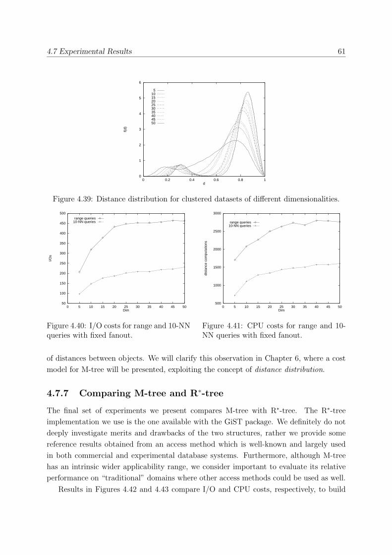
4.7 Experimental Results 61
0
1
2
3
4
5
6
0 0.2 0.4 0.6 0.8 1
f(d)
d
5101520253035404550
Figure 4.39: Distance distribution for clustered datasets of different dimensionalities.
50
100
150
200
250
300
350
400
450
500
0 5 10 15 20 25 30 35 40 45 50
I/Os
Dim
range queries10-NN queries
Figure 4.40: I/O costs for range and 10-NNqueries with fixed fanout.
500
1000
1500
2000
2500
3000
0 5 10 15 20 25 30 35 40 45 50
dist
ance
com
puta
tions
Dim
range queries10-NN queries
Figure 4.41: CPU costs for range and 10-NN queries with fixed fanout.
of distances between objects. We will clarify this observation in Chapter 6, where a cost
model for M-tree will be presented, exploiting the concept of distance distribution.
4.7.7 Comparing M-tree and R∗-tree
The final set of experiments we present compares M-tree with R∗-tree. The R∗-treeimplementation we use is the one available with the GiST package. We definitely do not
deeply investigate merits and drawbacks of the two structures, rather we provide some
reference results obtained from an access method which is well-known and largely used
in both commercial and experimental database systems. Furthermore, although M-tree
has an intrinsic wider applicability range, we consider important to evaluate its relative
performance on “traditional” domains where other access methods could be used as well.
Results in Figures 4.42 and 4.43 compare I/O and CPU costs, respectively, to build
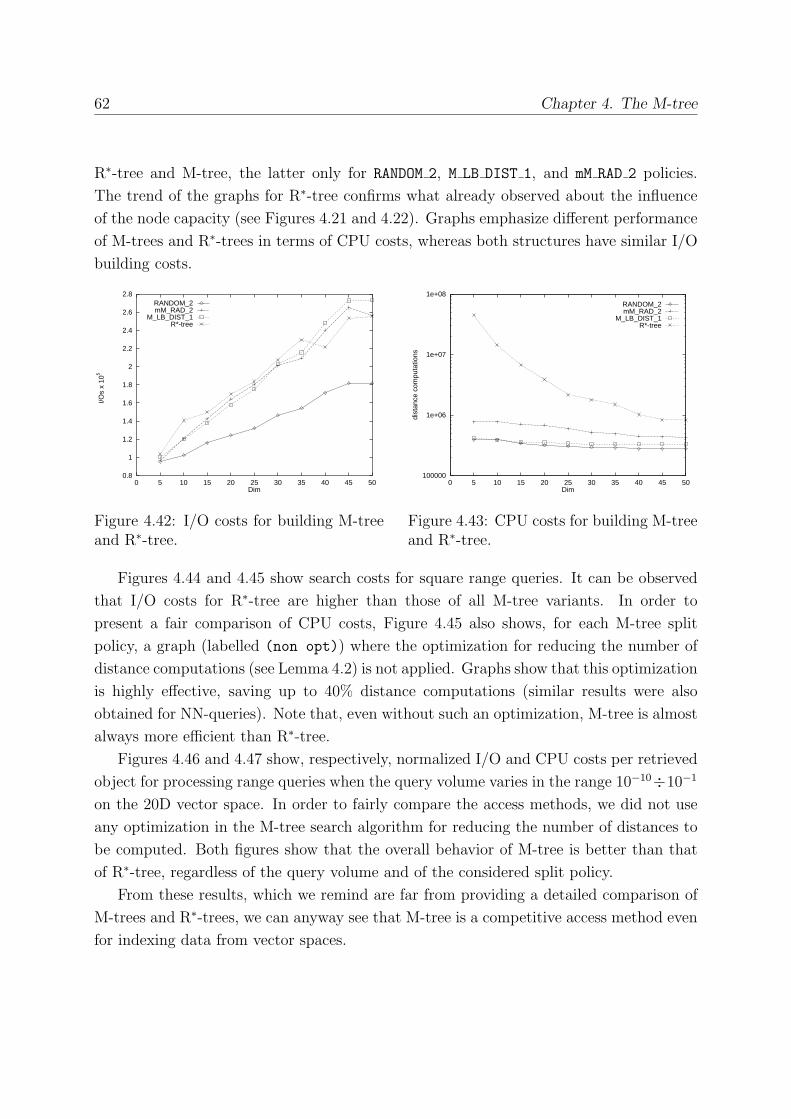
62 Chapter 4. The M-tree
R∗-tree and M-tree, the latter only for RANDOM 2, M LB DIST 1, and mM RAD 2 policies.
The trend of the graphs for R∗-tree confirms what already observed about the influenceof the node capacity (see Figures 4.21 and 4.22). Graphs emphasize different performance
of M-trees and R∗-trees in terms of CPU costs, whereas both structures have similar I/Obuilding costs.
0.8
1
1.2
1.4
1.6
1.8
2
2.2
2.4
2.6
2.8
0 5 10 15 20 25 30 35 40 45 50
I/Os
x 10
5
Dim
RANDOM_2mM_RAD_2
M_LB_DIST_1R*-tree
Figure 4.42: I/O costs for building M-treeand R∗-tree.
100000
1e+06
1e+07
1e+08
0 5 10 15 20 25 30 35 40 45 50
dist
ance
com
puta
tions
Dim
RANDOM_2mM_RAD_2
M_LB_DIST_1R*-tree
Figure 4.43: CPU costs for building M-treeand R∗-tree.
Figures 4.44 and 4.45 show search costs for square range queries. It can be observed
that I/O costs for R∗-tree are higher than those of all M-tree variants. In order to
present a fair comparison of CPU costs, Figure 4.45 also shows, for each M-tree split
policy, a graph (labelled (non opt)) where the optimization for reducing the number of
distance computations (see Lemma 4.2) is not applied. Graphs show that this optimization
is highly effective, saving up to 40% distance computations (similar results were also
obtained for NN-queries). Note that, even without such an optimization, M-tree is almost
always more efficient than R∗-tree.Figures 4.46 and 4.47 show, respectively, normalized I/O and CPU costs per retrieved
object for processing range queries when the query volume varies in the range 10−10÷10−1
on the 20D vector space. In order to fairly compare the access methods, we did not use
any optimization in the M-tree search algorithm for reducing the number of distances to
be computed. Both figures show that the overall behavior of M-tree is better than that
of R∗-tree, regardless of the query volume and of the considered split policy.From these results, which we remind are far from providing a detailed comparison of
M-trees and R∗-trees, we can anyway see that M-tree is a competitive access method evenfor indexing data from vector spaces.
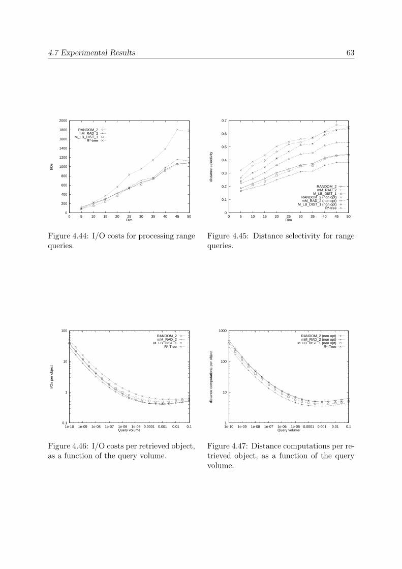
4.7 Experimental Results 63
0
200
400
600
800
1000
1200
1400
1600
1800
2000
0 5 10 15 20 25 30 35 40 45 50
I/Os
Dim
RANDOM_2mM_RAD_2
M_LB_DIST_1R*-tree
Figure 4.44: I/O costs for processing rangequeries.
0
0.1
0.2
0.3
0.4
0.5
0.6
0.7
0 5 10 15 20 25 30 35 40 45 50
dist
ance
sel
ectiv
ity
Dim
RANDOM_2mM_RAD_2
M_LB_DIST_1RANDOM_2 (non opt)mM_RAD_2 (non opt)
M_LB_DIST_1 (non opt)R*-tree
Figure 4.45: Distance selectivity for rangequeries.
0.1
1
10
100
1e-10 1e-09 1e-08 1e-07 1e-06 1e-05 0.0001 0.001 0.01 0.1
I/Os
per
obje
ct
Query volume
RANDOM_2mM_RAD_2
M_LB_DIST_1R*-Tree
Figure 4.46: I/O costs per retrieved object,as a function of the query volume.
1
10
100
1000
1e-10 1e-09 1e-08 1e-07 1e-06 1e-05 0.0001 0.001 0.01 0.1
dist
ance
com
puta
tions
per
obj
ect
Query volume
RANDOM_2 (non opt)mM_RAD_2 (non opt)
M_LB_DIST_1 (non opt)R*-Tree
Figure 4.47: Distance computations per re-trieved object, as a function of the queryvolume.


Chapter 5
Bulk Loading the M-tree
The incremental construction of an M-tree could lead, depending on the order of insertion
of the objects, to very different performances during the querying phase, as shown in
Section 4.7. In [CP98] we presented an algorithm to optimize the building of an M-tree
given a set of data objects. This “loading” of the tree can be done to speed-up the index
creation on a static database, or to reorganize the tree on a dynamic database, when
allowed by time constraints.
5.1 Bulk Loading Techniques
Typical spatial (multidimensional) index structures support random insertion, deletions
and updates, but, recently, there has been an increasing interest in bulk operations (i.e.
a series of operations executed atomically, without interruption by other actions). The
most common of such operations is the creation of an index from a given set of record
(bulk loading). A remarkable example is index creation to support index-based spatial
joins [LR94].
A great variety of bulk loading techniques have been proposed for R-trees. Most of
them [RL85, KF93, LLE97] sort the dataset using one-dimensional criteria, usually based
on the clustering properties of space-filling (e.g. Hilbert) curves. Only a few methods
[LL91, Gav94] exploit the “metric” properties of the dataset (i.e. relative distances be-
tween objects), and try to achieve a good clustering of the objects by iteratively improving
on the choice of clusters’ “centers”.
A generic algorithm to bulk loading multidimensional index structures (but the method
could be easily extended to metric indices) has been proposed in [vdBSW97]. The index
is built bottom-up by using buffer-trees. The major drawbacks of this technique are that
its performance still depends on the order in which data are inserted and its goal is to
reduce only I/O costs, thus ignoring CPU costs.
65
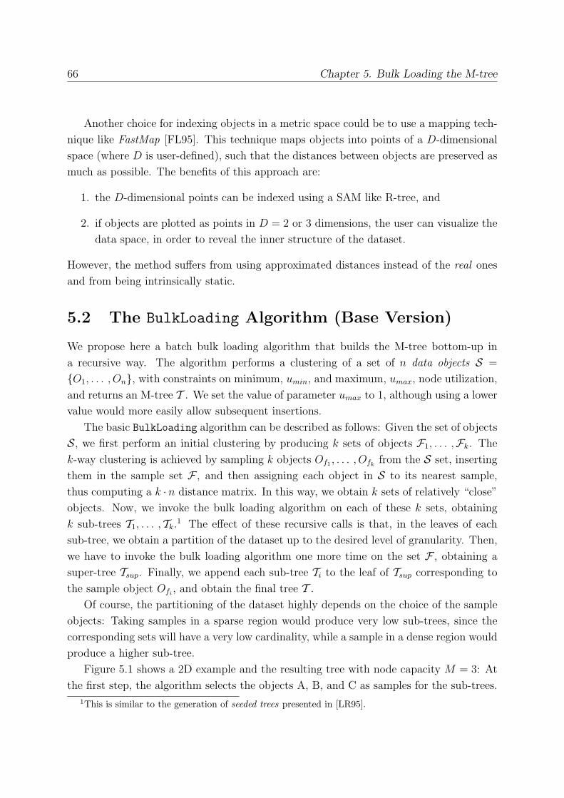
66 Chapter 5. Bulk Loading the M-tree
Another choice for indexing objects in a metric space could be to use a mapping tech-
nique like FastMap [FL95]. This technique maps objects into points of a D-dimensional
space (where D is user-defined), such that the distances between objects are preserved as
much as possible. The benefits of this approach are:
1. the D-dimensional points can be indexed using a SAM like R-tree, and
2. if objects are plotted as points in D = 2 or 3 dimensions, the user can visualize the
data space, in order to reveal the inner structure of the dataset.
However, the method suffers from using approximated distances instead of the real ones
and from being intrinsically static.
5.2 The BulkLoading Algorithm (Base Version)
We propose here a batch bulk loading algorithm that builds the M-tree bottom-up in
a recursive way. The algorithm performs a clustering of a set of n data objects S =
{O1, . . . , On}, with constraints on minimum, umin, and maximum, umax, node utilization,
and returns an M-tree T . We set the value of parameter umax to 1, although using a lower
value would more easily allow subsequent insertions.
The basic BulkLoading algorithm can be described as follows: Given the set of objects
S, we first perform an initial clustering by producing k sets of objects F1, . . . ,Fk. The
k-way clustering is achieved by sampling k objects Of1 , . . . , Ofkfrom the S set, inserting
them in the sample set F , and then assigning each object in S to its nearest sample,thus computing a k · n distance matrix. In this way, we obtain k sets of relatively “close”objects. Now, we invoke the bulk loading algorithm on each of these k sets, obtaining
k sub-trees T1, . . . , Tk.1 The effect of these recursive calls is that, in the leaves of each
sub-tree, we obtain a partition of the dataset up to the desired level of granularity. Then,
we have to invoke the bulk loading algorithm one more time on the set F , obtaining asuper-tree Tsup. Finally, we append each sub-tree Ti to the leaf of Tsup corresponding tothe sample object Ofi
, and obtain the final tree T .Of course, the partitioning of the dataset highly depends on the choice of the sample
objects: Taking samples in a sparse region would produce very low sub-trees, since the
corresponding sets will have a very low cardinality, while a sample in a dense region would
produce a higher sub-tree.
Figure 5.1 shows a 2D example and the resulting tree with node capacity M = 3: At
the first step, the algorithm selects the objects A, B, and C as samples for the sub-trees.
1This is similar to the generation of seeded trees presented in [LR95].
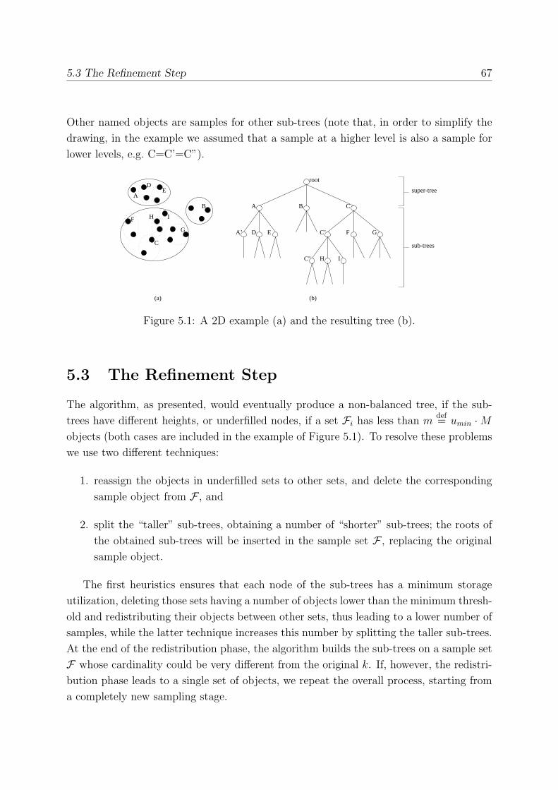
5.3 The Refinement Step 67
Other named objects are samples for other sub-trees (note that, in order to simplify the
drawing, in the example we assumed that a sample at a higher level is also a sample for
lower levels, e.g. C=C’=C”).
B
IF
C
H
G
A
DE
B
root
G
C
F
H IC"
C’D E
A
A’
sub-trees
super-tree
(a) (b)
Figure 5.1: A 2D example (a) and the resulting tree (b).
5.3 The Refinement Step
The algorithm, as presented, would eventually produce a non-balanced tree, if the sub-
trees have different heights, or underfilled nodes, if a set Fi has less than mdef= umin ·M
objects (both cases are included in the example of Figure 5.1). To resolve these problems
we use two different techniques:
1. reassign the objects in underfilled sets to other sets, and delete the corresponding
sample object from F , and
2. split the “taller” sub-trees, obtaining a number of “shorter” sub-trees; the roots of
the obtained sub-trees will be inserted in the sample set F , replacing the originalsample object.
The first heuristics ensures that each node of the sub-trees has a minimum storage
utilization, deleting those sets having a number of objects lower than the minimum thresh-
old and redistributing their objects between other sets, thus leading to a lower number of
samples, while the latter technique increases this number by splitting the taller sub-trees.
At the end of the redistribution phase, the algorithm builds the sub-trees on a sample set
F whose cardinality could be very different from the original k. If, however, the redistri-
bution phase leads to a single set of objects, we repeat the overall process, starting from
a completely new sampling stage.
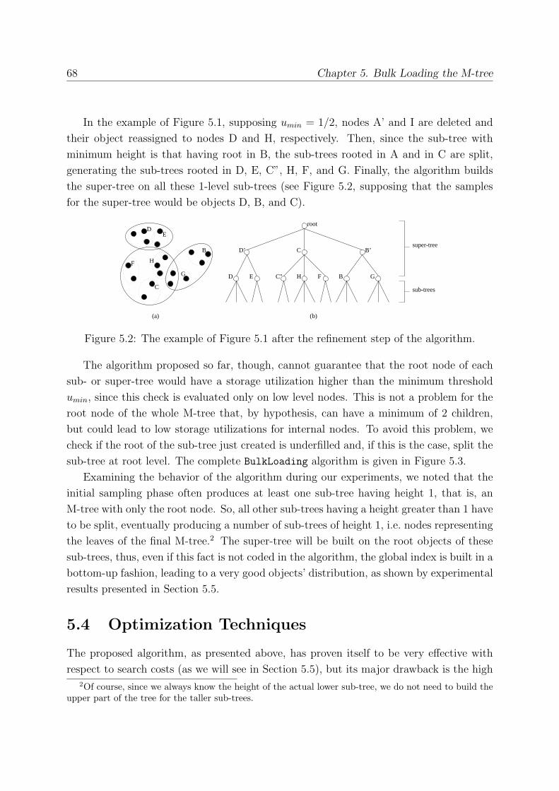
68 Chapter 5. Bulk Loading the M-tree
In the example of Figure 5.1, supposing umin = 1/2, nodes A’ and I are deleted and
their object reassigned to nodes D and H, respectively. Then, since the sub-tree with
minimum height is that having root in B, the sub-trees rooted in A and in C are split,
generating the sub-trees rooted in D, E, C”, H, F, and G. Finally, the algorithm builds
the super-tree on all these 1-level sub-trees (see Figure 5.2, supposing that the samples
for the super-tree would be objects D, B, and C).
F
C
G
E
B
D
C" H F
C
D E
D’
B G
B’
root
H
super-tree
sub-trees
(a) (b)
Figure 5.2: The example of Figure 5.1 after the refinement step of the algorithm.
The algorithm proposed so far, though, cannot guarantee that the root node of each
sub- or super-tree would have a storage utilization higher than the minimum threshold
umin, since this check is evaluated only on low level nodes. This is not a problem for the
root node of the whole M-tree that, by hypothesis, can have a minimum of 2 children,
but could lead to low storage utilizations for internal nodes. To avoid this problem, we
check if the root of the sub-tree just created is underfilled and, if this is the case, split the
sub-tree at root level. The complete BulkLoading algorithm is given in Figure 5.3.
Examining the behavior of the algorithm during our experiments, we noted that the
initial sampling phase often produces at least one sub-tree having height 1, that is, an
M-tree with only the root node. So, all other sub-trees having a height greater than 1 have
to be split, eventually producing a number of sub-trees of height 1, i.e. nodes representing
the leaves of the final M-tree.2 The super-tree will be built on the root objects of these
sub-trees, thus, even if this fact is not coded in the algorithm, the global index is built in a
bottom-up fashion, leading to a very good objects’ distribution, as shown by experimental
results presented in Section 5.5.
5.4 Optimization Techniques
The proposed algorithm, as presented above, has proven itself to be very effective with
respect to search costs (as we will see in Section 5.5), but its major drawback is the high2Of course, since we always know the height of the actual lower sub-tree, we do not need to build the
upper part of the tree for the taller sub-trees.
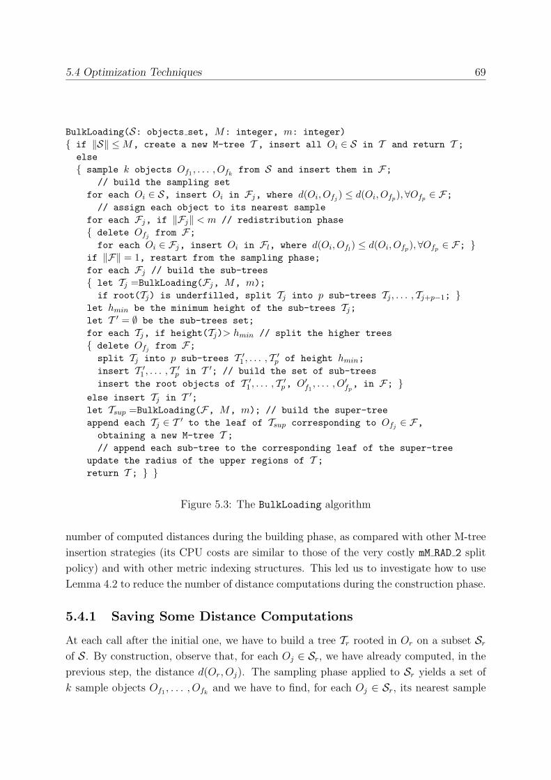
5.4 Optimization Techniques 69
BulkLoading(S: objects set, M: integer, m: integer){ if ‖S‖ ≤M, create a new M-tree T , insert all Oi ∈ S in T and return T ;
else{ sample k objects Of1 , . . . , Ofk
from S and insert them in F;// build the sampling set
for each Oi ∈ S, insert Oi in Fj, where d(Oi, Ofj ) ≤ d(Oi, Ofp),∀Ofp ∈ F;// assign each object to its nearest sample
for each Fj, if ‖Fj‖ < m // redistribution phase{ delete Ofj from F;
for each Oi ∈ Fj, insert Oi in Fl, where d(Oi, Ofl) ≤ d(Oi, Ofp),∀Ofp ∈ F; }
if ‖F‖ = 1, restart from the sampling phase;for each Fj // build the sub-trees{ let Tj =BulkLoading(Fj, M, m);
if root(Tj) is underfilled, split Tj into p sub-trees Tj , . . . , Tj+p−1; }let hmin be the minimum height of the sub-trees Tj;let T ′ = ∅ be the sub-trees set;for each Tj, if height(Tj)> hmin // split the higher trees{ delete Ofj from F;
split Tj into p sub-trees T ′1 , . . . , T ′
p of height hmin;insert T ′
1 , . . . , T ′p in T ′; // build the set of sub-trees
insert the root objects of T ′1 , . . . , T ′
p, O′f1
, . . . , O′fp, in F; }
else insert Tj in T ′;let Tsup =BulkLoading(F, M, m); // build the super-treeappend each Tj ∈ T ′ to the leaf of Tsup corresponding to Ofj ∈ F,
obtaining a new M-tree T ;// append each sub-tree to the corresponding leaf of the super-tree
update the radius of the upper regions of T ;return T ; } }
Figure 5.3: The BulkLoading algorithm
number of computed distances during the building phase, as compared with other M-tree
insertion strategies (its CPU costs are similar to those of the very costly mM RAD 2 split
policy) and with other metric indexing structures. This led us to investigate how to use
Lemma 4.2 to reduce the number of distance computations during the construction phase.
5.4.1 Saving Some Distance Computations
At each call after the initial one, we have to build a tree Tr rooted in Or on a subset Srof S. By construction, observe that, for each Oj ∈ Sr, we have already computed, in theprevious step, the distance d(Or, Oj). The sampling phase applied to Sr yields a set ofk sample objects Of1 , . . . , Ofk
and we have to find, for each Oj ∈ Sr, its nearest sample
70 Chapter 5. Bulk Loading the M-tree
object. Suppose O∗f is the nearest sample for object Oj obtained so far, and the distance
between Oj and a sample Ofp has to be computed: Since the value | d(Oj, Or)−d(Or, Ofp) |is a lower bound on d(Oj, Ofp), if d(Oj, O
∗f ) ≤| d(Oj, Or)−d(Or, Ofp) |, we can safely avoid
to compute d(Oj, Ofp), because this would surely be greater than d(Oj, O∗f ). The root
object, thus, acts as a vantage point for the computation of the distance matrix [Sha77].
This technique has two major limitations:
1. its application is possible only during the construction of sub-trees, whereas a lot
of distance computations are performed after the initial sampling phase (where no
distance has been computed yet) and during the construction of the super-tree, and
2. the use of the root object as a vantage point is not very effective, since it is likely that
it lies in the “center” of the cluster constituted by the set Sr, while it is suggested[Sha77] that vantage points should be multiple and far from the center of the cluster.
These considerations led us to consider a further optimization technique.
5.4.2 Saving More Distance Computations
In the base version of BulkLoading, we do not compute the relative distances between
sample objects, since it is clear that the nearest sample of such objects will be the sample
itself. If, though, we compute such distances, the sample objects can play the role of
multiple vantage points, like the root object in Section 5.4.1. In this case, however, the
sample objects are not crowded near the center of the cluster, thus leading to a more
efficient distance pruning. Experimental results will show if the overhead introduced by
the computation of the relative distances between the sample objects can result in a lower
number of computed distances. The global algorithm for the distance matrix computation
is shown in Figure 5.4.
Figures 5.5 and 5.6 show the results for both optimization techniques in terms of
percentage of distance computations saving and of total computed distances, respectively,
as a function of the space dimensionality (in the Figures BulkLoading0 refers to the
original algorithm, BulkLoading1 to the first optimization technique, while BulkLoading2
uses both optimization techniques). Here and in the experiments of Section 5.5, we will
use the same datasets and values used in Section 4.7.
The second optimization achieves far better results than the first one, reaching a 70%
saving for D = 5. The decreasing trend of distance computations saving is essentially due
to two factors:
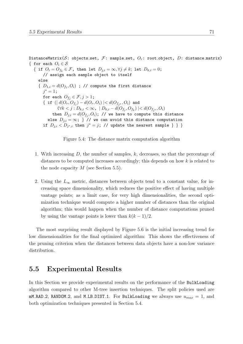
5.5 Experimental Results 71
DistanceMatrix(S: objects set, F: sample set, Or: root object, D: distance matrix){ for each Oi ∈ S{ if Oi = Ofk
∈ F, then let Dj,i =∞,∀j = k; let Dk,i = 0;// assign each sample object to itself
else{ D1,i = d(Of1 , Oi) ; // compute the first distance
j∗ = 1;for each Ofj ∈ F , j > 1;{ if (| d(Or, Ofj )− d(Or, Oi) |< d(Ofj∗ , Oi) and
(∀k < j : Dk,i <∞, | Dk,i − d(Ofj , Ofk) |< d(Ofj∗ , Oi)
then Dj,i = d(Ofj , Oi); // we have to compute this distanceelse Dj,i =∞; } // we can avoid this distance computation
if Dj,i < Dj∗,i then j∗ = j; // update the nearest sample } } }
Figure 5.4: The distance matrix computation algorithm
1. With increasing D, the number of samples, k, decreases, so that the percentage of
distances to be computed increases accordingly; this depends on how k is related to
the node capacity M (see Section 5.5).
2. Using the L∞ metric, distances between objects tend to a constant value, for in-
creasing space dimensionality, which reduces the positive effect of having multiple
vantage points; as a limit case, for very high dimensionalities, the second opti-
mization technique would compute a higher number of distances than the original
algorithm; this would happen when the number of distance computations pruned
by using the vantage points is lower than k(k − 1)/2.
The most surprising result displayed by Figure 5.6 is the initial increasing trend for
low dimensionalities for the final optimized algorithm: This shows the effectiveness of
the pruning criterion when the distances between data objects have a non-low variance
distribution.
5.5 Experimental Results
In this Section we provide experimental results on the performance of the BulkLoading
algorithm compared to other M-tree insertion techniques. The split policies used are
mM RAD 2, RANDOM 2, and M LB DIST 1. For BulkLoading we always use umax = 1, and
both optimization techniques presented in Section 5.4.
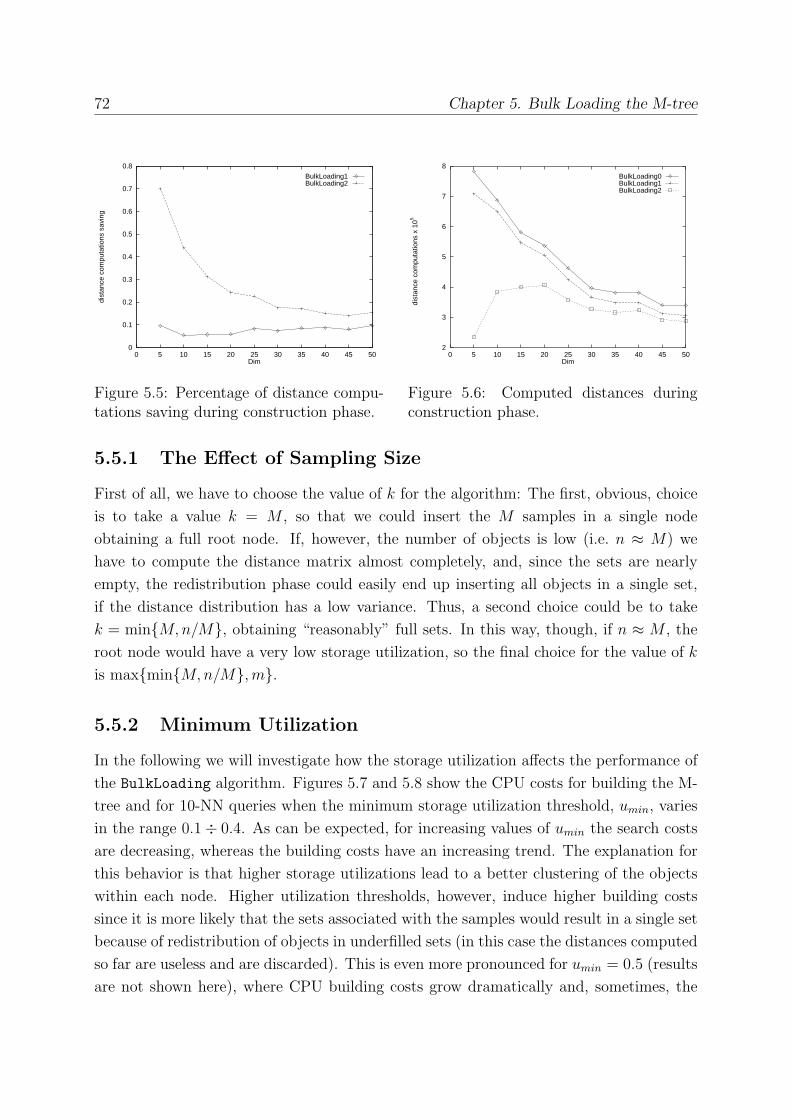
72 Chapter 5. Bulk Loading the M-tree
0
0.1
0.2
0.3
0.4
0.5
0.6
0.7
0.8
0 5 10 15 20 25 30 35 40 45 50
dist
ance
com
puta
tions
sav
ing
Dim
BulkLoading1BulkLoading2
Figure 5.5: Percentage of distance compu-tations saving during construction phase.
2
3
4
5
6
7
8
0 5 10 15 20 25 30 35 40 45 50
dist
ance
com
puta
tions
x 1
05
Dim
BulkLoading0BulkLoading1BulkLoading2
Figure 5.6: Computed distances duringconstruction phase.
5.5.1 The Effect of Sampling Size
First of all, we have to choose the value of k for the algorithm: The first, obvious, choice
is to take a value k = M , so that we could insert the M samples in a single node
obtaining a full root node. If, however, the number of objects is low (i.e. n ≈ M) we
have to compute the distance matrix almost completely, and, since the sets are nearly
empty, the redistribution phase could easily end up inserting all objects in a single set,
if the distance distribution has a low variance. Thus, a second choice could be to take
k = min{M,n/M}, obtaining “reasonably” full sets. In this way, though, if n ≈ M , the
root node would have a very low storage utilization, so the final choice for the value of k
is max{min{M,n/M},m}.
5.5.2 Minimum Utilization
In the following we will investigate how the storage utilization affects the performance of
the BulkLoading algorithm. Figures 5.7 and 5.8 show the CPU costs for building the M-
tree and for 10-NN queries when the minimum storage utilization threshold, umin, varies
in the range 0.1÷ 0.4. As can be expected, for increasing values of umin the search costs
are decreasing, whereas the building costs have an increasing trend. The explanation for
this behavior is that higher storage utilizations lead to a better clustering of the objects
within each node. Higher utilization thresholds, however, induce higher building costs
since it is more likely that the sets associated with the samples would result in a single set
because of redistribution of objects in underfilled sets (in this case the distances computed
so far are useless and are discarded). This is even more pronounced for umin = 0.5 (results
are not shown here), where CPU building costs grow dramatically and, sometimes, the
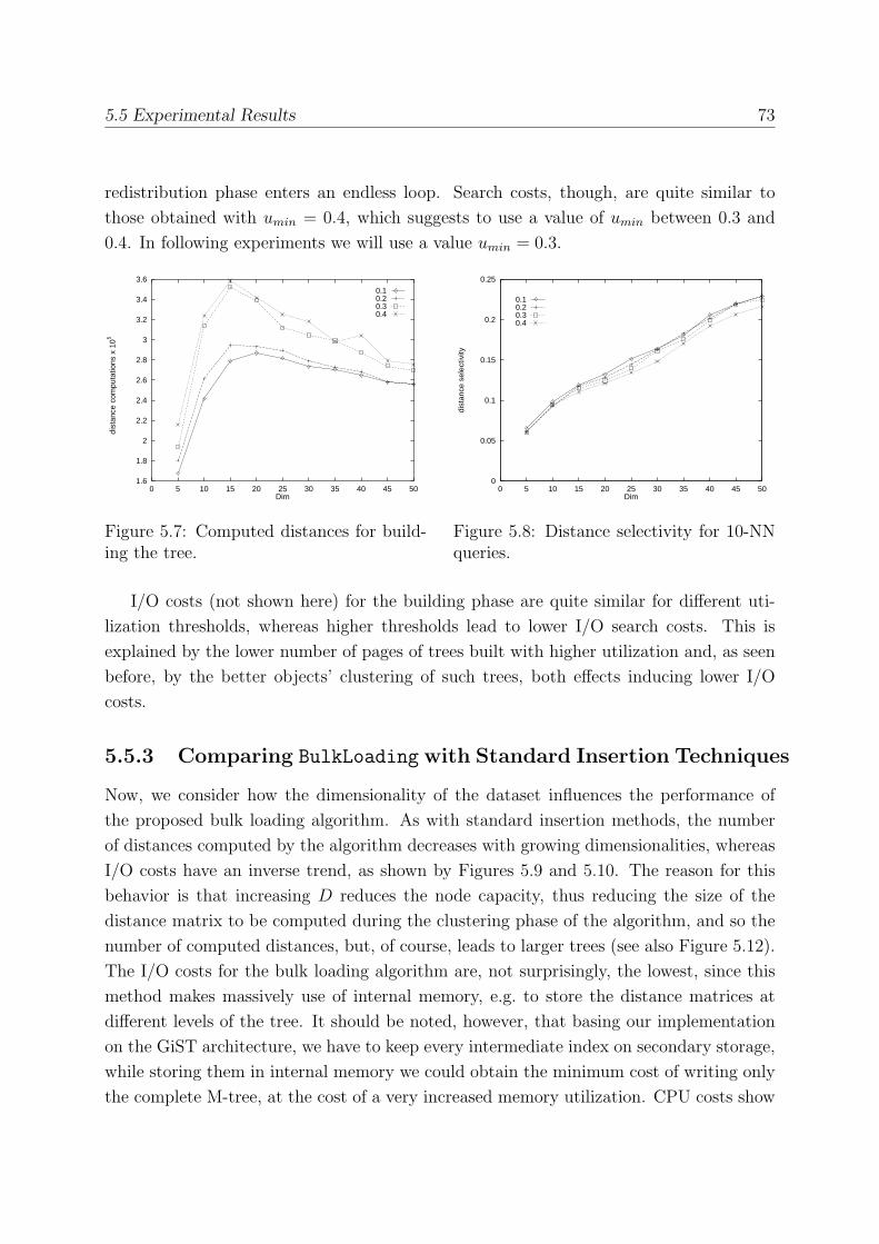
5.5 Experimental Results 73
redistribution phase enters an endless loop. Search costs, though, are quite similar to
those obtained with umin = 0.4, which suggests to use a value of umin between 0.3 and
0.4. In following experiments we will use a value umin = 0.3.
1.6
1.8
2
2.2
2.4
2.6
2.8
3
3.2
3.4
3.6
0 5 10 15 20 25 30 35 40 45 50
dist
ance
com
puta
tions
x 1
05
Dim
0.10.20.30.4
Figure 5.7: Computed distances for build-ing the tree.
0
0.05
0.1
0.15
0.2
0.25
0 5 10 15 20 25 30 35 40 45 50
dist
ance
sel
ectiv
ity
Dim
0.10.20.30.4
Figure 5.8: Distance selectivity for 10-NNqueries.
I/O costs (not shown here) for the building phase are quite similar for different uti-
lization thresholds, whereas higher thresholds lead to lower I/O search costs. This is
explained by the lower number of pages of trees built with higher utilization and, as seen
before, by the better objects’ clustering of such trees, both effects inducing lower I/O
costs.
5.5.3 Comparing BulkLoading with Standard Insertion Techniques
Now, we consider how the dimensionality of the dataset influences the performance of
the proposed bulk loading algorithm. As with standard insertion methods, the number
of distances computed by the algorithm decreases with growing dimensionalities, whereas
I/O costs have an inverse trend, as shown by Figures 5.9 and 5.10. The reason for this
behavior is that increasing D reduces the node capacity, thus reducing the size of the
distance matrix to be computed during the clustering phase of the algorithm, and so the
number of computed distances, but, of course, leads to larger trees (see also Figure 5.12).
The I/O costs for the bulk loading algorithm are, not surprisingly, the lowest, since this
method makes massively use of internal memory, e.g. to store the distance matrices at
different levels of the tree. It should be noted, however, that basing our implementation
on the GiST architecture, we have to keep every intermediate index on secondary storage,
while storing them in internal memory we could obtain the minimum cost of writing only
the complete M-tree, at the cost of a very increased memory utilization. CPU costs show
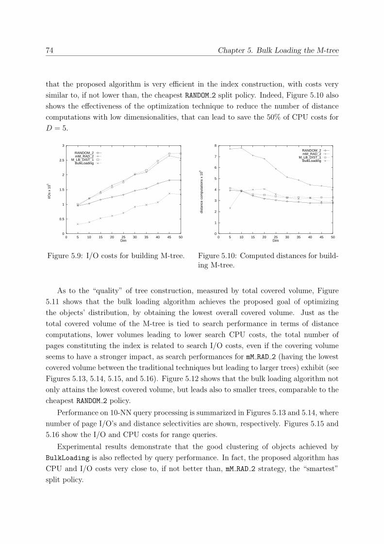
74 Chapter 5. Bulk Loading the M-tree
that the proposed algorithm is very efficient in the index construction, with costs very
similar to, if not lower than, the cheapest RANDOM 2 split policy. Indeed, Figure 5.10 also
shows the effectiveness of the optimization technique to reduce the number of distance
computations with low dimensionalities, that can lead to save the 50% of CPU costs for
D = 5.
0
0.5
1
1.5
2
2.5
3
0 5 10 15 20 25 30 35 40 45 50
I/Os
x 10
5
Dim
RANDOM_2mM_RAD_2
M_LB_DIST_1BulkLoading
Figure 5.9: I/O costs for building M-tree.
0
1
2
3
4
5
6
7
8
0 5 10 15 20 25 30 35 40 45 50
dist
ance
com
puta
tions
x 1
05
Dim
RANDOM_2mM_RAD_2
M_LB_DIST_1BulkLoading
Figure 5.10: Computed distances for build-ing M-tree.
As to the “quality” of tree construction, measured by total covered volume, Figure
5.11 shows that the bulk loading algorithm achieves the proposed goal of optimizing
the objects’ distribution, by obtaining the lowest overall covered volume. Just as the
total covered volume of the M-tree is tied to search performance in terms of distance
computations, lower volumes leading to lower search CPU costs, the total number of
pages constituting the index is related to search I/O costs, even if the covering volume
seems to have a stronger impact, as search performances for mM RAD 2 (having the lowest
covered volume between the traditional techniques but leading to larger trees) exhibit (see
Figures 5.13, 5.14, 5.15, and 5.16). Figure 5.12 shows that the bulk loading algorithm not
only attains the lowest covered volume, but leads also to smaller trees, comparable to the
cheapest RANDOM 2 policy.
Performance on 10-NN query processing is summarized in Figures 5.13 and 5.14, where
number of page I/O’s and distance selectivities are shown, respectively. Figures 5.15 and
5.16 show the I/O and CPU costs for range queries.
Experimental results demonstrate that the good clustering of objects achieved by
BulkLoading is also reflected by query performance. In fact, the proposed algorithm has
CPU and I/O costs very close to, if not better than, mM RAD 2 strategy, the “smartest”
split policy.
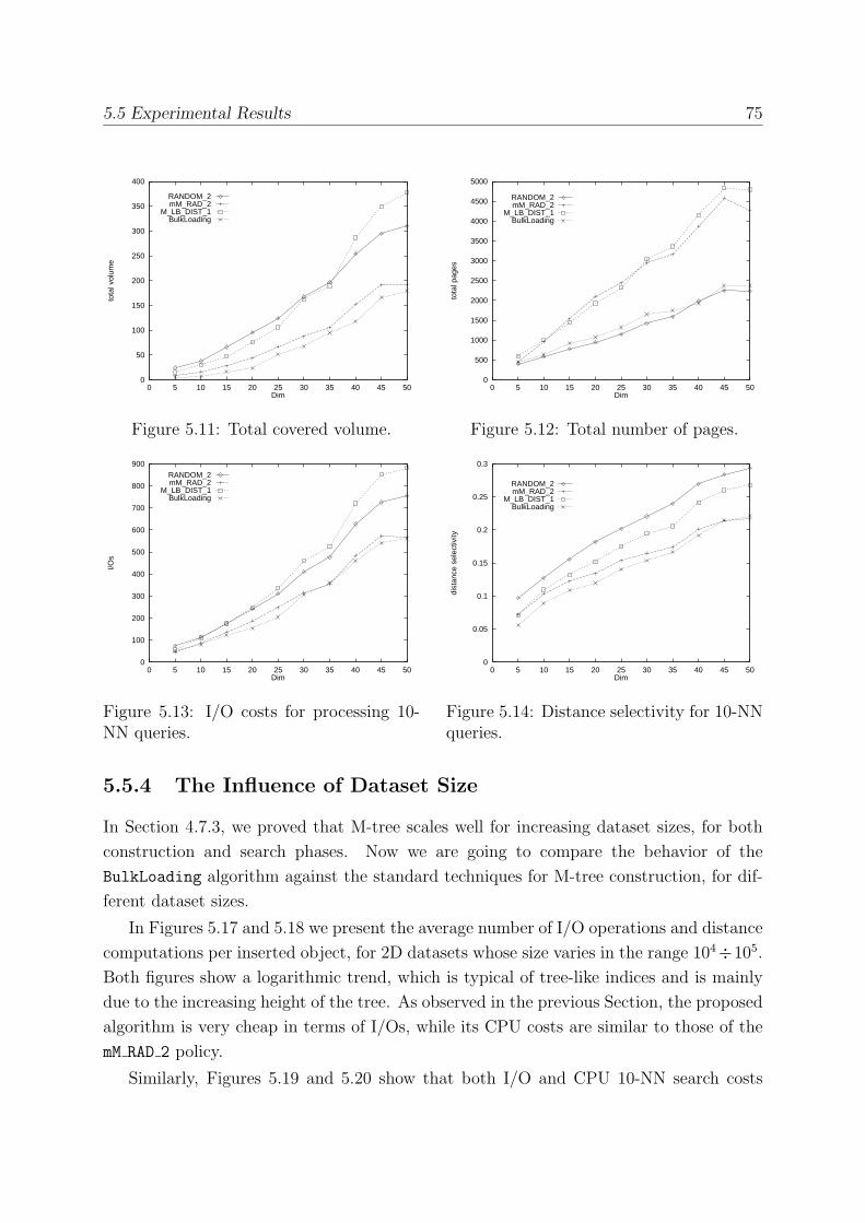
5.5 Experimental Results 75
0
50
100
150
200
250
300
350
400
0 5 10 15 20 25 30 35 40 45 50
tota
l vol
ume
Dim
RANDOM_2mM_RAD_2
M_LB_DIST_1BulkLoading
Figure 5.11: Total covered volume.
0
500
1000
1500
2000
2500
3000
3500
4000
4500
5000
0 5 10 15 20 25 30 35 40 45 50
tota
l pag
es
Dim
RANDOM_2mM_RAD_2
M_LB_DIST_1BulkLoading
Figure 5.12: Total number of pages.
0
100
200
300
400
500
600
700
800
900
0 5 10 15 20 25 30 35 40 45 50
I/Os
Dim
RANDOM_2mM_RAD_2
M_LB_DIST_1BulkLoading
Figure 5.13: I/O costs for processing 10-NN queries.
0
0.05
0.1
0.15
0.2
0.25
0.3
0 5 10 15 20 25 30 35 40 45 50
dist
ance
sel
ectiv
ity
Dim
RANDOM_2mM_RAD_2
M_LB_DIST_1BulkLoading
Figure 5.14: Distance selectivity for 10-NNqueries.
5.5.4 The Influence of Dataset Size
In Section 4.7.3, we proved that M-tree scales well for increasing dataset sizes, for both
construction and search phases. Now we are going to compare the behavior of the
BulkLoading algorithm against the standard techniques for M-tree construction, for dif-
ferent dataset sizes.
In Figures 5.17 and 5.18 we present the average number of I/O operations and distance
computations per inserted object, for 2D datasets whose size varies in the range 104÷105.
Both figures show a logarithmic trend, which is typical of tree-like indices and is mainly
due to the increasing height of the tree. As observed in the previous Section, the proposed
algorithm is very cheap in terms of I/Os, while its CPU costs are similar to those of the
mM RAD 2 policy.
Similarly, Figures 5.19 and 5.20 show that both I/O and CPU 10-NN search costs
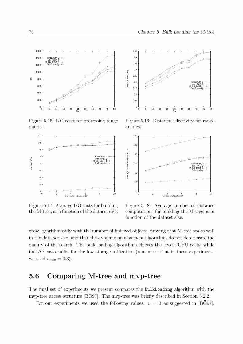
76 Chapter 5. Bulk Loading the M-tree
0
200
400
600
800
1000
1200
1400
1600
0 5 10 15 20 25 30 35 40 45 50
I/Os
Dim
RANDOM_2mM_RAD_2
M_LB_DIST_1BulkLoading
Figure 5.15: I/O costs for processing rangequeries.
0
0.05
0.1
0.15
0.2
0.25
0.3
0.35
0.4
0.45
0 5 10 15 20 25 30 35 40 45 50
dist
ance
sel
ectiv
ity
Dim
RANDOM_2mM_RAD_2
M_LB_DIST_1BulkLoading
Figure 5.16: Distance selectivity for rangequeries.
3
4
5
6
7
8
9
10
11
0 2 4 6 8 10
aver
age
I/Os
number of objects x 104
RANDOM_2mM_RAD_2
M_LB_DIST_1BulkLoading
Figure 5.17: Average I/O costs for buildingthe M-tree, as a function of the dataset size.
0
20
40
60
80
100
120
0 2 4 6 8 10
aver
age
dist
ance
com
puta
tions
number of objects x 104
RANDOM_2mM_RAD_2
M_LB_DIST_1BulkLoading
Figure 5.18: Average number of distancecomputations for building the M-tree, as afunction of the dataset size.
grow logarithmically with the number of indexed objects, proving that M-tree scales well
in the data set size, and that the dynamic management algorithms do not deteriorate the
quality of the search. The bulk loading algorithm achieves the lowest CPU costs, while
its I/O costs suffer for the low storage utilization (remember that in these experiments
we used umin = 0.3).
5.6 Comparing M-tree and mvp-tree
The final set of experiments we present compares the BulkLoading algorithm with the
mvp-tree access structure [BO97]. The mvp-tree was briefly described in Section 3.2.2.
For our experiments we used the following values: v = 3 as suggested in [BO97],
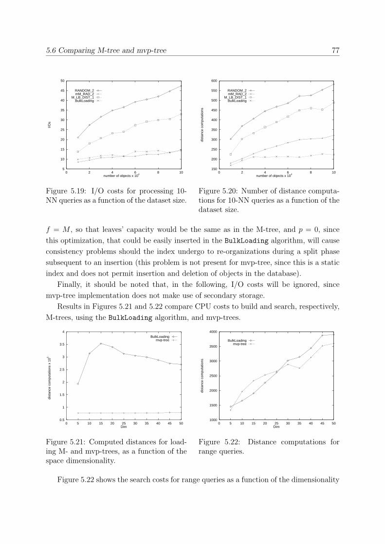
5.6 Comparing M-tree and mvp-tree 77
5
10
15
20
25
30
35
40
45
50
0 2 4 6 8 10
I/Os
number of objects x 104
RANDOM_2mM_RAD_2
M_LB_DIST_1BulkLoading
Figure 5.19: I/O costs for processing 10-NN queries as a function of the dataset size.
150
200
250
300
350
400
450
500
550
600
0 2 4 6 8 10
dist
ance
com
puta
tions
number of objects x 104
RANDOM_2mM_RAD_2
M_LB_DIST_1BulkLoading
Figure 5.20: Number of distance computa-tions for 10-NN queries as a function of thedataset size.
f = M , so that leaves’ capacity would be the same as in the M-tree, and p = 0, since
this optimization, that could be easily inserted in the BulkLoading algorithm, will cause
consistency problems should the index undergo to re-organizations during a split phase
subsequent to an insertion (this problem is not present for mvp-tree, since this is a static
index and does not permit insertion and deletion of objects in the database).
Finally, it should be noted that, in the following, I/O costs will be ignored, since
mvp-tree implementation does not make use of secondary storage.
Results in Figures 5.21 and 5.22 compare CPU costs to build and search, respectively,
M-trees, using the BulkLoading algorithm, and mvp-trees.
0.5
1
1.5
2
2.5
3
3.5
4
0 5 10 15 20 25 30 35 40 45 50
dist
ance
com
puta
tions
x 1
05
Dim
BulkLoadingmvp-tree
Figure 5.21: Computed distances for load-ing M- and mvp-trees, as a function of thespace dimensionality.
1000
1500
2000
2500
3000
3500
4000
0 5 10 15 20 25 30 35 40 45 50
dist
ance
com
puta
tions
Dim
BulkLoadingmvp-tree
Figure 5.22: Distance computations forrange queries.
Figure 5.22 shows the search costs for range queries as a function of the dimensionality
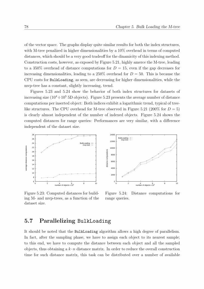
78 Chapter 5. Bulk Loading the M-tree
of the vector space. The graphs display quite similar results for both the index structures,
with M-tree penalized in higher dimensionalities by a 10% overhead in terms of computed
distances, which should be a very good tradeoff for the dinamicity of this indexing method.
Construction costs, however, as exposed by Figure 5.21, highly amerce the M-tree, leading
to a 350% overhead of distance computations for D = 15, even if the gap decreases for
increasing dimensionalities, leading to a 250% overhead for D = 50. This is because the
CPU costs for BulkLoading, as seen, are decreasing for higher dimensionalities, while the
mvp-tree has a constant, slightly increasing, trend.
Figures 5.23 and 5.24 show the behavior of both index structures for datasets of
increasing size (104÷105 5D objects). Figure 5.23 presents the average number of distance
computations per inserted object: Both indices exhibit a logarithmic trend, typical of tree-
like structures. The CPU overhead for M-tree observed in Figure 5.21 (200% for D = 5)
is clearly almost independent of the number of indexed objects. Figure 5.24 shows the
computed distances for range queries: Performances are very similar, with a difference
independent of the dataset size.
6
8
10
12
14
16
18
20
22
24
26
28
0 2 4 6 8 10
aver
age
dist
ance
com
puta
tions
number of objects x 104
BulkLoadingmvp-tree
Figure 5.23: Computed distances for build-ing M- and mvp-trees, as a function of thedataset size.
0
2000
4000
6000
8000
10000
12000
14000
0 2 4 6 8 10
dist
ance
com
puta
tions
number of objects x 104
BulkLoadingmvp-tree
Figure 5.24: Distance computations forrange queries.
5.7 Parallelizing BulkLoading
It should be noted that the BulkLoading algorithm allows a high degree of parallelism.
In fact, after the sampling phase, we have to assign each object to its nearest sample;
to this end, we have to compute the distance between each object and all the sampled
objects, thus obtaining a k ·n distance matrix. In order to reduce the overall constructiontime for such distance matrix, this task can be distributed over a number of available

5.7 Parallelizing BulkLoading 79
processors, each processor computing a row (i.e. the distance between a sample object
and all the data objects), a column (the distance between a data object and all sample
objects), or even a single cell of the matrix, if the number of available processors is very
high. It should be noted, though, that the optimization techniques presented in Section
5.4 allow the parallelization of the task of computing the distance matrix only by way of
rows, i.e. computing the distances between a sample object and all the data objects.
The assignment of each object to its nearest sample could also be distributed over a
number of processors, every processor taking charge of the task of finding the minimum
value in an array, this array being a column of the distance matrix. Moreover, the building
of each sub-tree could be assigned to a separate processor, thus spreading the utilization
of the available processors, since the construction of a sub-tree could entail the building
of sub-sub-trees and so on. Finally, the task of appending the sub-trees to the leaves of
the super-tree could also be spanned over a number of processors.

Chapter 6
Cost Models for Metric Trees
Although application of metric trees to concrete indexing problems has been proved to be
effective [Bri95, BYO97, CPZ97], even on “traditional” vector spaces (see also Section 3.2),
no theoretical analysis able to predict and justify their performance results is available
nowadays. In other terms, no cost model for metric trees exists yet, which makes their
applicability to a specific dataset still a matter of chance. For instance, given a large
set of keywords extracted from a text, to be compared using the edit distance, and an
input (query) keyword Q, which is the expected (CPU and I/O) cost to retrieve the,
say, 20 nearest neighbors of Q, that is, the 20 strings which are “closest” to Q? Being
able to answer questions like this is relevant for database design, query processing, and
optimization, since it would provide us with the capability of understanding and tuning a
metric access method, and will make it possible to apply optimizers’ technology to metric
query processing too. In [CPZ98a] we introduced the first average-case cost model for
metric trees, showing how our approach can be applied to derive cost models for the M-tree
and the vp-tree [Yia93] index structures. Then, in [CNP99], we extended the average-
case models to derive an effective query-sensitive model, i.e. a model able to change its
estimates according to the “position” of the query object.
6.1 Cost Models for Spatial Access Methods
Prior to [CPZ98a], no specific work had addressed the problem of estimating costs for
queries over generic metric spaces. However, in order to introduce our cost model for
metric trees, it is useful to review what has been done in recent years for the case of
vector (Cartesian) spaces, which are a subset of metric spaces, with a major focus on the
performance of R-tree and its variants.
In [KF93] the authors present a model to estimate I/O costs for range queries as a
function of the geometric characteristics of the R-tree’s nodes, under the assumption of
81
82 Chapter 6. Cost Models for Metric Trees
uniform distribution of both data and query points. The basic result for this cost model
is the following:
Lemma 6.1
The probability that a node N of the R-tree is accessed in a point query is given by its
volume.
Proof: This results immediately follows from the assumption of the uniform distribution
of point queries in the D-dimensional hypercube. In this case, the probability that a
random point falls in a hyper-rectangular region is given by the volume of that region.
Therefore, the expected I/O costs for a point query is given by the sum of the covered
volume of all the index nodes. ✷
The result of Lemma 6.1 is then extended to window queries by the following:
Lemma 6.2
The probability that a node N of the R-tree is accessed in a window query is given by the
volume of the hyper-rectangle obtained by “inflating” the node region by the dimension
of the query region in each dimension.
Proof: To prove this result is sufficient to show that the probability that the node region
and the query region overlap is equal to the probability that a random point is inside the
“inflated” region. ✷
Above results are extended in [FK94], by using concepts of fractal theory [Man77],
to derive a cost model for R-tree, which does not depend on the assumption of uniform
distribution of query points. The obtained cost model is tree-independent, in the sense
that no statistics on the tree are used, but only information on the fractal dimension of
the dataset and on the effective average capacity of a tree node.
The two previous models for R-tree only provide estimates for average costs. Within
the context of query optimization, particular relevance have query-sensitive cost models,
i.e. models able to change their estimates according to the “position” of the query object.
In [TS96], a query-sensitive model for predicting I/O costs of range queries on R-tree
is presented; the model is based on a D-dimensional histogram which approximates the
distribution of the dataset over a D-dimensional vector space. Using such information,
the model can predict costs for a specific query, by using the density of points around the
query object.
In [PM97], the authors extend the model of [KF93] to predict average I/O costs
for nearest neighbor queries. The proposed model is limited to the real plane with the
Euclidean distance and provides an estimate of the distance between the query point and
its nearest neighbor and a lower and an upper bound on the number of accessed pages.
6.2 The Distance Distribution 83
Finally, in [BBKK97] a complete cost model for nearest neighbor queries over generic
multi-dimensional spaces indexed by an X-tree is presented. The model relies on the
assumption of uniform distribution of query points and exploits statistics on the tree
nodes, thus being tree-dependent. Boundary effects are considered by using the concept
of Minkowski sum, leading to quite accurate estimates, even in high dimensions.
6.2 The Distance Distribution
It has to be remarked that all the models presented in Section 6.1 exploit information
about data distribution, i.e. about the position of objects within the considered vector
space:
• In [KF93] and in [BBKK97] uniformly distributed datasets are considered.
• In [FK94] the fractal dimension of the dataset is used.
• In [TS96] the density of points is stored for different regions of the space.
It is clear that, in a generic metric space, no information on data distribution can be used.
Therefore, above models cannot be applied to metric trees.1
Hence, in order to derive a cost model for metric trees, we pursue an approach which
does not rely on data distribution, rather it takes a more general view, able to deal whith
generic metric spaces, which can be characterized by the following positions:
1. The only information derivable from the analysis of a metric dataset is (an estimate
of) the distance distribution of objects. No information on data distribution is used.
2. A biased query model (the distribution of query objects is equal to that of data
objects) is considered, with query objects which do not necessarily belong to the
indexed dataset.
We claim that the distance distribution is the correct counterpart of data distribution
used for vector spaces, since it is the “natural” way to characterize a metric dataset. As
to the biased query model, which apparently contradicts the position that no knowledge
of the data distribution is assumed, we clarify this point by precisely defining our working
scenario.
First of all we have to extend the concept of metric space.
1In principle, concepts of fractal theory can be applied to metric spaces. However, their introductionto develop a fractal cost model is left as subject for future work.
84 Chapter 6. Cost Models for Metric Trees
Definition 6.1 (Bounded random metric space)
A bounded random metric (brm) space is a quadruple M = (D, d, d+, S), where D and
d are as usual, d+ is a finite upper bound on distance values, and S is a measure of
probability over (a suitable Borel field defined on) D. ✷
To help intuition, we slightly abuse terminology and call S the data distribution over
D. Although S has no specific role in our cost model (we do not need to know S and
never use it), its existence is postulated both for formal reasons and to account for the
nature of the observed datasets (see Section 6.3.1).
Example 6.1
([0, 1]D, L2,√D,U([0, 1]D)) is the brm space characterized by an uniform distribution of
points over the D-dimensional unit hyper-cube, and where distance between points is
measured by the Euclidean (L2) metric. ✷
Example 6.2
(Σm, Ledit,m, S) is the brm space whose domain is the set of all the strings of length up
to m over the Σ alphabet, whose distance is measured by the edit (Levenshtein) metric
(see Example 2.3), and with data distribution S, here left unspecified. ✷
Definition 6.2 (Distance distribution)
The (overall) distribution of distances over D is defined as:
F (x) = Pr{d(O1,O2) ≤ x} (6.1)
where O1 and O2 are two (independent) S-distributed random points of D. For eachOi ∈ D, the relative distance distribution, rdd, of Oi is obtained by simply setting
O1 = Oi in Equation 6.1, i.e:
FOi(x) = Pr{d(Oi,O2) ≤ x} (6.2)
✷
Intuitively, FOi(x) represents the fraction of objects in D, sampled according to the
S data distribution, whose distance from Oi does not exceed x. For what follows it is
useful to regard FOias the Oi’s “viewpoint” of the D domain, as determined by d and S.
The fact that different objects can have different viewpoints is the general rule. Even for
an uniform distribution over a bounded Cartesian domain, the center’s viewpoint is not
the same as the viewpoint an object close to the boundary has. In order to measure how
much two viewpoints are (dis-)similar, we introduce the concept of discrepancy.
6.2 The Distance Distribution 85
Definition 6.3 (Discrepancy)
The discrepancy of the two rdds FOiand FOj
is defined as:
δ(FOi, FOj
) =1
d+
∫ d+
0
|FOi(x)− FOj
(x)| dx (6.3)
✷
The discrepancy of any pair of rdds is a real number in the unit interval [0, 1], and equals
0 iff FOiand FOj
are the same (which does not imply, however, that Oi ≡ Oj). Note that
δ is a metric on the functional space F = {FOi: Oi ∈ D}, as it can be easily verified.
Consider now the case where both O1 and O2 are random points. Under this view,
∆def= δ(FO1 , FO2) is a random variable, and G∆(y) = Pr{∆ ≤ y} is the probability that
the discrepancy of two (random) rdds is not larger than y. The higher, for a given y,
G∆(y) is, the more likely is that two rdds FOiand FOj
“behave” the same, up to an y
level of discrepancy. Therefore, if G∆(y) ≈ 1 for a “low” y value, we can say that the
brm spaceM from which G is derived is somewhat “homogeneous” as to the viewpoints
that objects in D, weighted according to the S distribution, have. This observation is
captured by introducing an index of homogeneity for brm spaces.
Definition 6.4 (Homogeneity of Viewpoints)
The index of “Homogeneity of Viewpoints” of a brm spaceM is defined as:
HV (M) =
∫ 1
0
G∆(y) dy = 1− E[∆] (6.4)
✷
Example 6.3
Consider the brm spaceM = ({0, 1}D ∪ {(0.5, . . . , 0.5)}, L∞, 1, U), where the domain isthe D-dimensional binary hypercube extended with the “midpoint” C = (0.5, . . . , 0.5),
points are uniformly distributed, and L∞(Oi, Oj) = maxDk=1{|Oi[k] − Oj[k]|}. For all
Oi, Oj ∈ {0, 1}D it is δ(FOi, FOj
) = 0, whereas δ(FOi, FC) = 1/2− 1/(2D + 1). It follows
that G∆(y) = (22D + 1)/(2D + 1)2 for 0 ≤ y < 1/2 − 1/(2D + 1), and G∆(y) = 1 for
1/2− 1/(2D + 1) ≤ y ≤ 1. Therefore
HV (M) = 1− 22D − 2D
(2D + 1)3D→∞−→ 1
For instance, when D = 10, it is HV (M) ≈ 1− 0.97× 10⁻³ ≈ 0.999. Since all points butC have the same view ofM, even for moderately large values of D the presence of C has
a negligible effect on HV (M). ✷
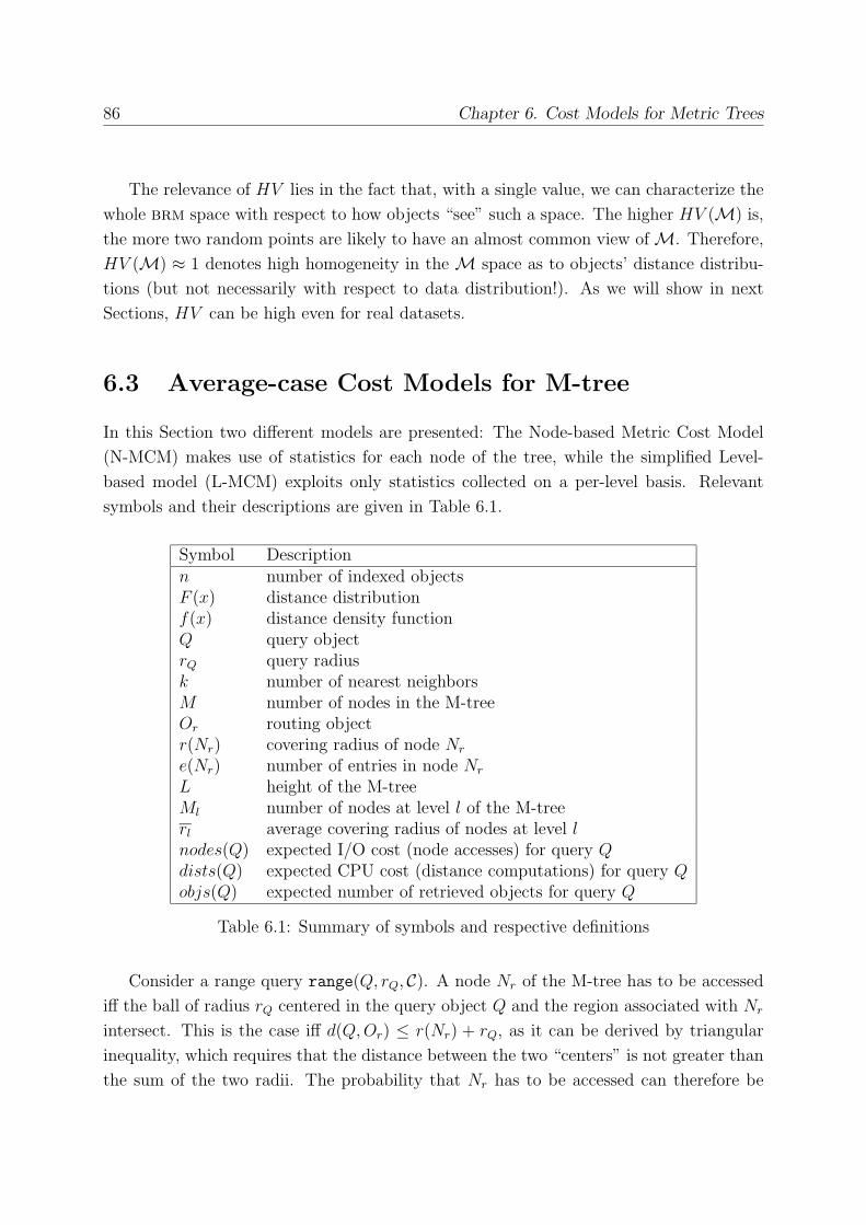
86 Chapter 6. Cost Models for Metric Trees
The relevance of HV lies in the fact that, with a single value, we can characterize the
whole brm space with respect to how objects “see” such a space. The higher HV (M) is,
the more two random points are likely to have an almost common view ofM. Therefore,
HV (M) ≈ 1 denotes high homogeneity in theM space as to objects’ distance distribu-
tions (but not necessarily with respect to data distribution!). As we will show in next
Sections, HV can be high even for real datasets.
6.3 Average-case Cost Models for M-tree
In this Section two different models are presented: The Node-based Metric Cost Model
(N-MCM) makes use of statistics for each node of the tree, while the simplified Level-
based model (L-MCM) exploits only statistics collected on a per-level basis. Relevant
symbols and their descriptions are given in Table 6.1.
Symbol Descriptionn number of indexed objectsF (x) distance distributionf(x) distance density functionQ query objectrQ query radiusk number of nearest neighborsM number of nodes in the M-treeOr routing objectr(Nr) covering radius of node Nr
e(Nr) number of entries in node Nr
L height of the M-treeMl number of nodes at level l of the M-treerl average covering radius of nodes at level lnodes(Q) expected I/O cost (node accesses) for query Qdists(Q) expected CPU cost (distance computations) for query Qobjs(Q) expected number of retrieved objects for query Q
Table 6.1: Summary of symbols and respective definitions
Consider a range query range(Q, rQ, C). A node Nr of the M-tree has to be accessed
iff the ball of radius rQ centered in the query object Q and the region associated with Nr
intersect. This is the case iff d(Q,Or) ≤ r(Nr) + rQ, as it can be derived by triangular
inequality, which requires that the distance between the two “centers” is not greater than
the sum of the two radii. The probability that Nr has to be accessed can therefore be
6.3 Average-case Cost Models for M-tree 87
expressed as:2
Pr{node Nr is accessed} = Pr{d(Q,O) ≤ r(Nr) + rQ} = FQ(r(Nr) + rQ) (6.5)
where the uncertainty is due to the position in the space of the routing object of Nr, here
considered to be a random point.
Equation 6.5 is the starting point for all the proposed cost models. However, it is easy
to see that it is unusable in this form. In fact, the probability that a node is accessed
is given as a function of the distance distribution relative to the query object Q, that is
obviously unknown at query execution time. Hence, what is needed is a way to somehow
approximate the unknown distance distribution FQ. In the following we will present the
basic assumptions that led us to develop two different average-case cost models for M-tree.
6.3.1 Dealing with Database Instances
A database instance O = {O1, . . . , On} of D is, according to our view, an n-sized sampleof objects, selected according to the (unknown) S data distribution over D. From this
sample, the basic information we can derive about the brm spaceM is an estimate of F ,
denoted F n, represented by the n× n matrix of pairwise distances between objects in O.As we previously saw, for estimating the cost of a query (either range or nearest
neighbors), the best thing would be to know FQ, i.e. the rdd of the query object itself.
However, in the general case this is a hopeless alternative, since Q is not restricted to
belong to O. What if we use F n in place of FQ? As long as the two distributions behave
almost the same, we do not expect relevant estimate errors from any cost model we could
devise, provided the model correctly uses F n.
In order to verify the above possibility, we computed the HV index for several syn-
thetic and real datasets, summarized in Table 6.2. The clustered datasets consist of
D-dimensional vectors normally-distributed (with σ=0.1) in 10 clusters over the unit hy-
percube. Text datasets in Table 6.2 are sets of keywords extracted from 5 masterpieces
of Italian literature.
For all these datasets we observed HV values always above 0.98, which justifies the
following assumption we make for deriving our cost model:
Assumption 6.1
The homogeneity of viewpoints index, HV , is “high” (close to 1), and the relative dis-
tance distribution of a query object Q is well approximated by the sampled F n distance
distribution. ✷
2The radius r(Nr) is not defined for the root node. To obviate this we assume that the root has radiusr(Nroot) = d+.
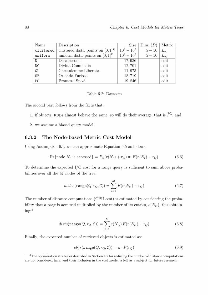
88 Chapter 6. Cost Models for Metric Trees
Name Description Size Dim. (D) Metricclustered clustered distr. points on [0, 1]D 104 − 105 5− 50 L∞uniform uniform distr. points on [0, 1]D 104 − 105 5− 50 L∞D Decamerone 17, 936 editDC Divina Commedia 12, 701 editGL Gerusalemme Liberata 11, 973 editOF Orlando Furioso 18, 719 editPS Promessi Sposi 19, 846 edit
Table 6.2: Datasets
The second part follows from the facts that:
1. if objects’ rdds almost behave the same, so will do their average, that is F n, and
2. we assume a biased query model.
6.3.2 The Node-based Metric Cost Model
Using Assumption 6.1, we can approximate Equation 6.5 as follows:
Pr{node Nr is accessed} = FQ(r(Nr) + rQ) ≈ F (r(Nr) + rQ) (6.6)
To determine the expected I/O cost for a range query is sufficient to sum above proba-
bilities over all the M nodes of the tree:
nodes(range(Q, rQ, C)) =M∑i=1
F (r(Nri) + rQ) (6.7)
The number of distance computations (CPU cost) is estimated by considering the proba-
bility that a page is accessed multiplied by the number of its entries, e(Nri), thus obtain-
ing:3
dists(range(Q, rQ, C)) =M∑i=1
e(Nri)F (r(Nri
) + rQ) (6.8)
Finally, the expected number of retrieved objects is estimated as:
objs(range(Q, rQ, C)) = n · F (rQ) (6.9)
3The optimization strategies described in Section 4.2 for reducing the number of distance computationsare not considered here, and their inclusion in the cost model is left as a subject for future research.
6.3 Average-case Cost Models for M-tree 89
Let us now consider the case of a nearest neighbors query, NN(Q, k, C), on the assump-tion that k < n. As a first step we determine the expected distance between the query
object and its k-th nearest neighbor, which depends on the distance distribution FQ. Let
nnQ,k be the random variable standing for the distance of the k-th nearest neighbor of Q
to the query object itself. The probability that nnQ,k is at most r equals the probability
that at least k objects are inside the ball of radius r centered in Q, that is:
PQ,k(r)def= Pr{nnQ,k ≤ r} = (6.10)
=n∑
i=k
(n
i
)Pr{d(Q,O) ≤ r}i Pr{d(Q,O) > r}n−i =
=n∑
i=k
(n
i
)FQ(r)
i(1− FQ(r))n−i =
=n∑i=0
(n
i
)FQ(r)
i(1− FQ(r))n−i −
k−1∑i=0
(n
i
)FQ(r)
i(1− FQ(r))n−i =
= 1−k−1∑i=0
(n
i
)FQ(r)
i(1− FQ(r))n−i ≈ 1−
k−1∑i=0
(n
i
)F (r)i(1− F (r))n−i
The density function pQ,k(r) is obtained by taking the derivative of PQ,k(r):
pQ,k(r) =d
drPQ,k(r) ≈
d
dr
(1−
k−1∑i=0
(n
i
)F (r)i(1− F (r))n−i
)= (6.11)
= −k−1∑i=0
(n
i
) [i · F (r)i−1 f(r)(1− F (r))n−i − (n− i)F (r)if(r)(1− F (r))n−i−1
]=
=k−1∑i=0
(n
i
)F (r)i−1f(r)(1− F (r))n−i−1 [(n− i) F (r)− i(1− F (r))] =
=k−1∑i=0
(n
i
)F (r)i−1f(r)(1− F (r))n−i−1(nF (r)− i)
and the expected k-th nearest neighbor distance is computed by integrating pQ,k(r) over
all r values:
E[nnQ,k] =
∫ d+
0
r · pQ,k(r) dr = (6.12)
= |r PQ,k(r)|d+
0 −∫ d+
0
PQ,k(r) dr = d+ −∫ d+
0
PQ,k(r) dr
90 Chapter 6. Cost Models for Metric Trees
For k = 1, above results simplify as follows:
PQ,1(r) ≈ 1− (1− F (r))n (6.13)
pQ,1(r) =d
drPQ,1(r) ≈ n f(r) (1− F (r))n−1 (6.14)
E[nnQ,1] =
∫ d+
0
r · pQ,1(r) dr ≈∫ d+
0
r n f(r) (1− F (r))n−1 dr = (6.15)
= − |r (1− F (r))n|d+
0 +
∫ d+
0
(1− F (r))n dr =
∫ d+
0
(1− F (r))n dr
and reduce to those derived in [BBKK97] for vector spaces and Euclidean distance. We
remark, however, that above formulas are suitable for generic metric spaces, since they
do not require the computation of any “Cartesian volume”, as done in [BBKK97].
Equation 6.15 shows that the expected nearest neighbor distance can be obtained by
integrating over all the possible distance values the n-th power of the complement to 1 of
the distance distribution. Note that limn→∞(1 − F (r))n = 0, thus E[nnQ,1] goes to zero
when the number of objects tends to infinity, as intuition may suggest.
The expected number of page reads can now be obtained by integrating Equation
6.7 over all radius values, each value weighted by its probability to occur, as given by
Equation 6.11. For the case k = 1 we obtain
nodes(NN(Q, 1, C)) =
∫ d+
0
nodes(range(Q, r, C)) pQ,1(r) dr ≈ (6.16)
≈∫ d+
0
M∑i=1
F (r(Nri) + r) n f(r) (1− F (r))n−1 dr
The same principle is applied to determine the expected number of computed distances,
for which the number of entries in each node has to be considered:
dists(NN(Q, 1, C)) =
∫ d+
0
dists(range(Q, r, C)) pQ,1(r) dr ≈ (6.17)
≈∫ d+
0
M∑i=1
e(Nri) F (r(Nri
) + r) n f(r) (1− F (r))n−1 dr
6.3.3 The Level-based Metric Cost Model
The basic problem with N-MCM is that mantaining statistics for every node of the tree
requires O(M) = O(n) space and the computation of expected values has the same
complexity, thus can be very time consuming when the index is (very) large. To obviate
this, we consider a simplified model, called L-MCM, which uses only average information
6.3 Average-case Cost Models for M-tree 91
collected for each level of the M-tree. This will intuitively lead to a lower accuracy with
respect to N-MCM, but, as shown in Section 6.3.4, estimates are still accurate enough.
For each level l of the tree (l = 1, . . . , L, with the root at level 1 and leaves at level
L), L-MCM just uses two information: Ml (the number of nodes at level l), and rl (the
average value of the covering radius considering all the nodes at level l). Given these
statistics, and referring to Equation 6.7, the number of pages accessed by a range query
can be estimated as:
nodes(range(Q, rQ, C)) ≈L∑l=1
Ml F (rl + rQ) (6.18)
Similarly, we can estimate CPU costs as:
dists(range(Q, rQ, C)) ≈L∑l=1
Ml+1 F (rl + rQ) (6.19)
where ML+1def= n is the number of indexed objects. Compared to Equation 6.8, we have
exploited the simple observation that the number of nodes at a given level equals the
number of entries at the next upper level of the tree.
Correspondingly, I/O and CPU costs for a NN(Q, 1, C) query are estimated as follows:
nodes(NN(Q, 1, C)) ≈∫ d+
0
L∑l=1
Ml F (rl + r) n f(r) (1− F (r))n−1 dr (6.20)
dists(NN(Q, 1, C)) ≈∫ d+
0
L∑l=1
Ml+1 F (rl + r) n f(r) (1− F (r))n−1 dr (6.21)
6.3.4 Experimental Evaluation
In order to evaluate the accuracy of the presented cost models, we ran several experiments
on both synthetic and real datasets, as described in Table 6.2. Estimates were compared
with actual results obtained by the M-tree, which was built using the BulkLoading algo-
rithm described in Chapter 5 with a node size of 4 Kbytes and a minimum node utilization
of 30%.
The first set of experiments concerns the clustered datasets, and investigates ac-
curacy of estimates as a function of the dimensionality D of the space. The distance
distribution is approximated by an equi-width histogram with 100 bins, respectively stor-
ing the values of F n(0.01), F n(0.02), and so on.
Figures 6.1 and 6.2 show estimated and real CPU costs and the relative errors (aver-
aged over 1000 queries), respectively, for range queries with radius D√0.01/2 as a function
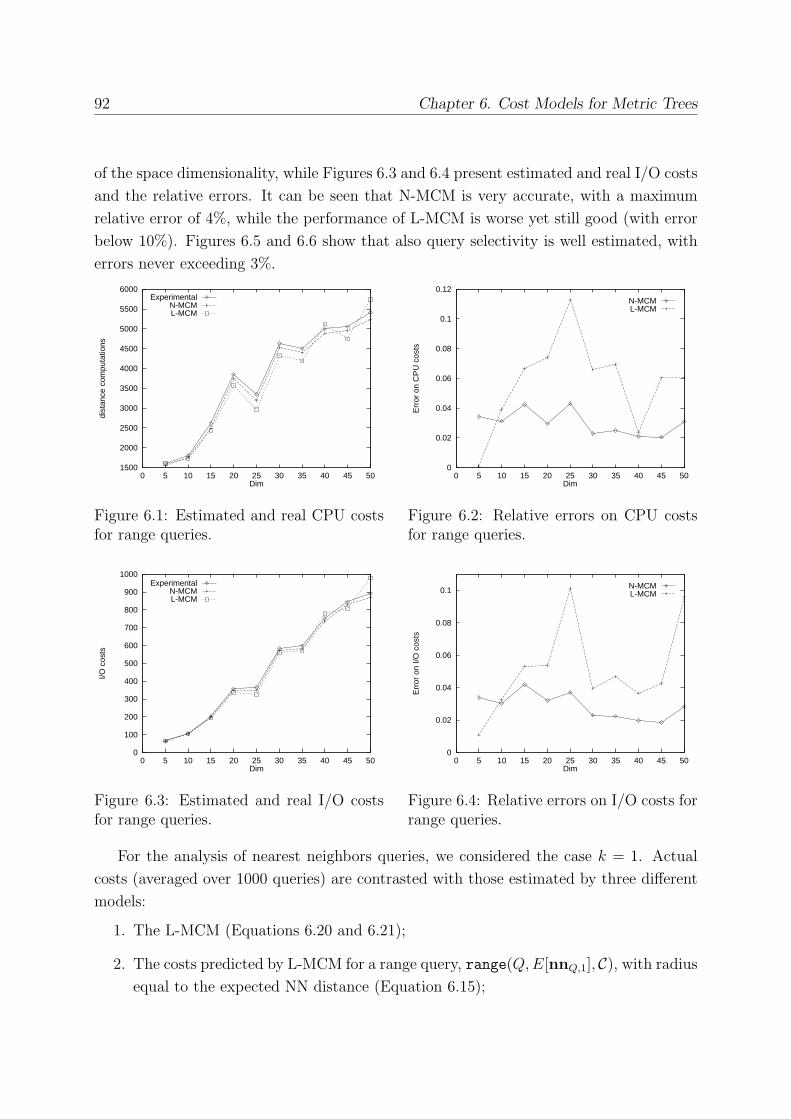
92 Chapter 6. Cost Models for Metric Trees
of the space dimensionality, while Figures 6.3 and 6.4 present estimated and real I/O costs
and the relative errors. It can be seen that N-MCM is very accurate, with a maximum
relative error of 4%, while the performance of L-MCM is worse yet still good (with error
below 10%). Figures 6.5 and 6.6 show that also query selectivity is well estimated, with
errors never exceeding 3%.
1500
2000
2500
3000
3500
4000
4500
5000
5500
6000
0 5 10 15 20 25 30 35 40 45 50
dist
ance
com
puta
tions
Dim
ExperimentalN-MCML-MCM
Figure 6.1: Estimated and real CPU costsfor range queries.
0
0.02
0.04
0.06
0.08
0.1
0.12
0 5 10 15 20 25 30 35 40 45 50
Err
or o
n C
PU
cos
ts
Dim
N-MCML-MCM
Figure 6.2: Relative errors on CPU costsfor range queries.
0
100
200
300
400
500
600
700
800
900
1000
0 5 10 15 20 25 30 35 40 45 50
I/O c
osts
Dim
ExperimentalN-MCML-MCM
Figure 6.3: Estimated and real I/O costsfor range queries.
0
0.02
0.04
0.06
0.08
0.1
0 5 10 15 20 25 30 35 40 45 50
Err
or o
n I/O
cos
ts
Dim
N-MCML-MCM
Figure 6.4: Relative errors on I/O costs forrange queries.
For the analysis of nearest neighbors queries, we considered the case k = 1. Actual
costs (averaged over 1000 queries) are contrasted with those estimated by three different
models:
1. The L-MCM (Equations 6.20 and 6.21);
2. The costs predicted by L-MCM for a range query, range(Q,E[nnQ,1], C), with radiusequal to the expected NN distance (Equation 6.15);
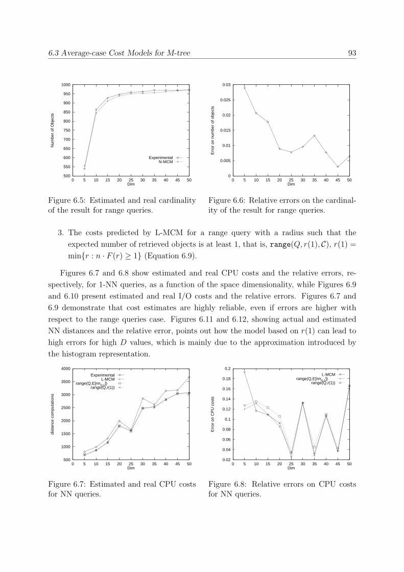
6.3 Average-case Cost Models for M-tree 93
500
550
600
650
700
750
800
850
900
950
1000
0 5 10 15 20 25 30 35 40 45 50
Num
ber
of O
bjec
ts
Dim
ExperimentalN-MCM
Figure 6.5: Estimated and real cardinalityof the result for range queries.
0
0.005
0.01
0.015
0.02
0.025
0.03
0 5 10 15 20 25 30 35 40 45 50
Err
or o
n nu
mbe
r of
obj
ects
Dim
Figure 6.6: Relative errors on the cardinal-ity of the result for range queries.
3. The costs predicted by L-MCM for a range query with a radius such that the
expected number of retrieved objects is at least 1, that is, range(Q, r(1), C), r(1) =min{r : n · F (r) ≥ 1} (Equation 6.9).
Figures 6.7 and 6.8 show estimated and real CPU costs and the relative errors, re-
spectively, for 1-NN queries, as a function of the space dimensionality, while Figures 6.9
and 6.10 present estimated and real I/O costs and the relative errors. Figures 6.7 and
6.9 demonstrate that cost estimates are highly reliable, even if errors are higher with
respect to the range queries case. Figures 6.11 and 6.12, showing actual and estimated
NN distances and the relative error, points out how the model based on r(1) can lead to
high errors for high D values, which is mainly due to the approximation introduced by
the histogram representation.
500
1000
1500
2000
2500
3000
3500
4000
0 5 10 15 20 25 30 35 40 45 50
dist
ance
com
puta
tions
Dim
ExperimentalL-MCM
range(Q,E[nnQ,1])range(Q,r(1))
Figure 6.7: Estimated and real CPU costsfor NN queries.
0.02
0.04
0.06
0.08
0.1
0.12
0.14
0.16
0.18
0.2
0 5 10 15 20 25 30 35 40 45 50
Err
or o
n C
PU
cos
ts
Dim
L-MCMrange(Q,E[nnQ,1])
range(Q,r(1))
Figure 6.8: Relative errors on CPU costsfor NN queries.
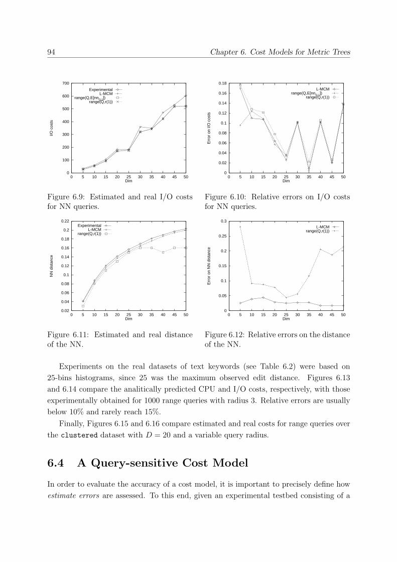
94 Chapter 6. Cost Models for Metric Trees
0
100
200
300
400
500
600
700
0 5 10 15 20 25 30 35 40 45 50
I/O c
osts
Dim
ExperimentalL-MCM
range(Q,E[nnQ,1])range(Q,r(1))
Figure 6.9: Estimated and real I/O costsfor NN queries.
0
0.02
0.04
0.06
0.08
0.1
0.12
0.14
0.16
0.18
0 5 10 15 20 25 30 35 40 45 50
Err
or o
n I/O
cos
ts
Dim
L-MCMrange(Q,E[nnQ,1])
range(Q,r(1))
Figure 6.10: Relative errors on I/O costsfor NN queries.
0.02
0.04
0.06
0.08
0.1
0.12
0.14
0.16
0.18
0.2
0.22
0 5 10 15 20 25 30 35 40 45 50
NN
dis
tanc
e
Dim
ExperimentalL-MCM
range(Q,r(1))
Figure 6.11: Estimated and real distanceof the NN.
0
0.05
0.1
0.15
0.2
0.25
0.3
0 5 10 15 20 25 30 35 40 45 50
Err
or o
n N
N d
ista
nce
Dim
L-MCMrange(Q,r(1))
Figure 6.12: Relative errors on the distanceof the NN.
Experiments on the real datasets of text keywords (see Table 6.2) were based on
25-bins histograms, since 25 was the maximum observed edit distance. Figures 6.13
and 6.14 compare the analitically predicted CPU and I/O costs, respectively, with those
experimentally obtained for 1000 range queries with radius 3. Relative errors are usually
below 10% and rarely reach 15%.
Finally, Figures 6.15 and 6.16 compare estimated and real costs for range queries over
the clustered dataset with D = 20 and a variable query radius.
6.4 A Query-sensitive Cost Model
In order to evaluate the accuracy of a cost model, it is important to precisely define how
estimate errors are assessed. To this end, given an experimental testbed consisting of a
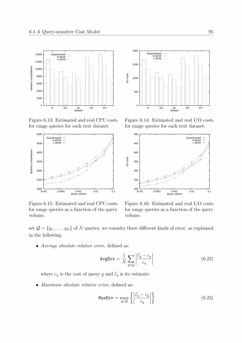
6.4 A Query-sensitive Cost Model 95
0
2000
4000
6000
8000
10000
12000
14000
D DC GL OF PS
dist
ance
com
puta
tions
dataset
ExperimentalN-MCML-MCM
Figure 6.13: Estimated and real CPU costsfor range queries for each text dataset.
0
500
1000
1500
2000
D DC GL OF PS
I/O c
osts
dataset
ExperimentalN-MCML-MCM
Figure 6.14: Estimated and real I/O costsfor range queries for each text dataset.
2000
2500
3000
3500
4000
4500
5000
1e-05 0.0001 0.001 0.01 0.1
dist
ance
com
puta
tions
Query volume
ExperimentalN-MCML-MCM
Figure 6.15: Estimated and real CPU costsfor range queries as a function of the queryvolume.
200
250
300
350
400
450
500
1e-05 0.0001 0.001 0.01 0.1
I/O c
osts
Query volume
ExperimentalN-MCML-MCM
Figure 6.16: Estimated and real I/O costsfor range queries as a function of the queryvolume.
set Q = {q1, . . . , qN} of N queries, we consider three different kinds of error, as explained
in the following.
• Average absolute relative error, defined as:
AvgErr =1
N
∑q∈Q
∣∣∣∣ cq − cqcq
∣∣∣∣ (6.22)
where cq is the cost of query q and cq is its estimate.
• Maximum absolute relative error, defined as:
MaxErr = maxq∈Q
{∣∣∣∣ cq − cqcq
∣∣∣∣} (6.23)
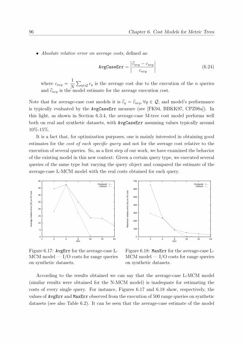
96 Chapter 6. Cost Models for Metric Trees
• Absolute relative error on average costs, defined as:
AvgCaseErr =
∣∣∣∣ cavg − cavgcavg
∣∣∣∣ (6.24)
where cavg =1
N
∑q∈Q cq is the average cost due to the execution of the n queries
and cavg is the model estimate for the average execution cost.
Note that for average-case cost models it is cq = cavg,∀q ∈ Q, and model’s performanceis typically evaluated by the AvgCaseErr measure (see [FK94, BBKK97, CPZ98a]). In
this light, as shown in Section 6.3.4, the average-case M-tree cost model performs well
both on real and synthetic datasets, with AvgCaseErr assuming values typically around
10%-15%.
It is a fact that, for optimization purposes, one is mainly interested in obtaining good
estimates for the cost of each specific query and not for the average cost relative to the
execution of several queries. So, as a first step of our work, we have examined the behavior
of the existing model in this new context: Given a certain query type, we executed several
queries of the same type but varying the query object and compared the estimate of the
average-case L-MCM model with the real costs obtained for each query.
0
5
10
15
20
25
30
35
40
1 2 4 8 16 32 64
Ave
rage
rel
ativ
e er
ror
(%)
on I/
O c
ost
Dim
ClusteredUniform
Figure 6.17: AvgErr for the average-case L-MCM model — I/O costs for range querieson synthetic datasets.
0
100
200
300
400
500
600
700
1 2 4 8 16 32 64
Max
imum
rel
ativ
e er
ror
(%)
on I/
O c
ost
Dim
ClusteredUniform
Figure 6.18: MaxErr for the average-case L-MCM model — I/O costs for range querieson synthetic datasets.
According to the results obtained we can say that the average-case L-MCM model
(similar results were obtained for the N-MCM model) is inadequate for estimating the
costs of every single query. For instance, Figures 6.17 and 6.18 show, respectively, the
values of AvgErr and MaxErr observed from the execution of 500 range queries on synthetic
datasets (see also Table 6.2). It can be seen that the average-case estimate of the model
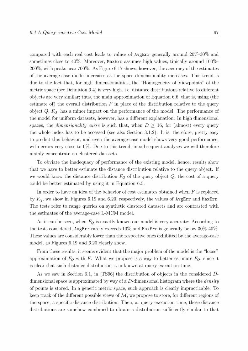
6.4 A Query-sensitive Cost Model 97
compared with each real cost leads to values of AvgErr generally around 20%-30% and
sometimes close to 40%. Moreover, MaxErr assumes high values, tipically around 100%-
200%, with peaks near 700%. As Figure 6.17 shows, however, the accuracy of the estimates
of the average-case model increases as the space dimensionality increases. This trend is
due to the fact that, for high dimensionalities, the “Homogeneity of Viewpoints” of the
metric space (see Definition 6.4) is very high, i.e. distance distributions relative to different
objects are very similar; thus, the main approximation of Equation 6.6, that is, using (the
estimate of) the overall distribution F in place of the distribution relative to the query
object Q, FQ, has a minor impact on the performance of the model. The performance of
the model for uniform datasets, however, has a different explanation: In high dimensional
spaces, the dimensionality curse is such that, when D ≥ 16, for (almost) every query
the whole index has to be accessed (see also Section 3.1.2). It is, therefore, pretty easy
to predict this behavior, and even the average-case model shows very good performance,
with errors very close to 0%. Due to this trend, in subsequent analyses we will therefore
mainly concentrate on clustered datasets.
To obviate the inadequacy of performance of the existing model, hence, results show
that we have to better estimate the distance distribution relative to the query object. If
we would know the distance distribution FQ of the query object Q, the cost of a query
could be better estimated by using it in Equation 6.5.
In order to have an idea of the behavior of cost estimates obtained when F is replaced
by FQ, we show in Figures 6.19 and 6.20, respectively, the values of AvgErr and MaxErr.
The tests refer to range queries on synthetic clustered datasets and are contrasted with
the estimates of the average-case L-MCM model.
As it can be seen, when FQ is exactly known our model is very accurate: According to
the tests considered, AvgErr rarely exceeds 10% and MaxErr is generally below 30%-40%.
These values are considerably lower than the respective ones exhibited by the average-case
model, as Figures 6.19 and 6.20 clearly show.
From these results, it seems evident that the major problem of the model is the “loose”
approximation of FQ with F . What we propose is a way to better estimate FQ, since it
is clear that such distance distribution is unknown at query execution time.
As we saw in Section 6.1, in [TS96] the distribution of objects in the considered D-
dimensional space is approximated by way of aD-dimensional histogram where the density
of points is stored. In a generic metric space, such approach is clearly impracticable: To
keep track of the different possible views ofM, we propose to store, for different regions of
the space, a specific distance distribution. Then, at query execution time, these distance
distributions are somehow combined to obtain a distribution sufficiently similar to that
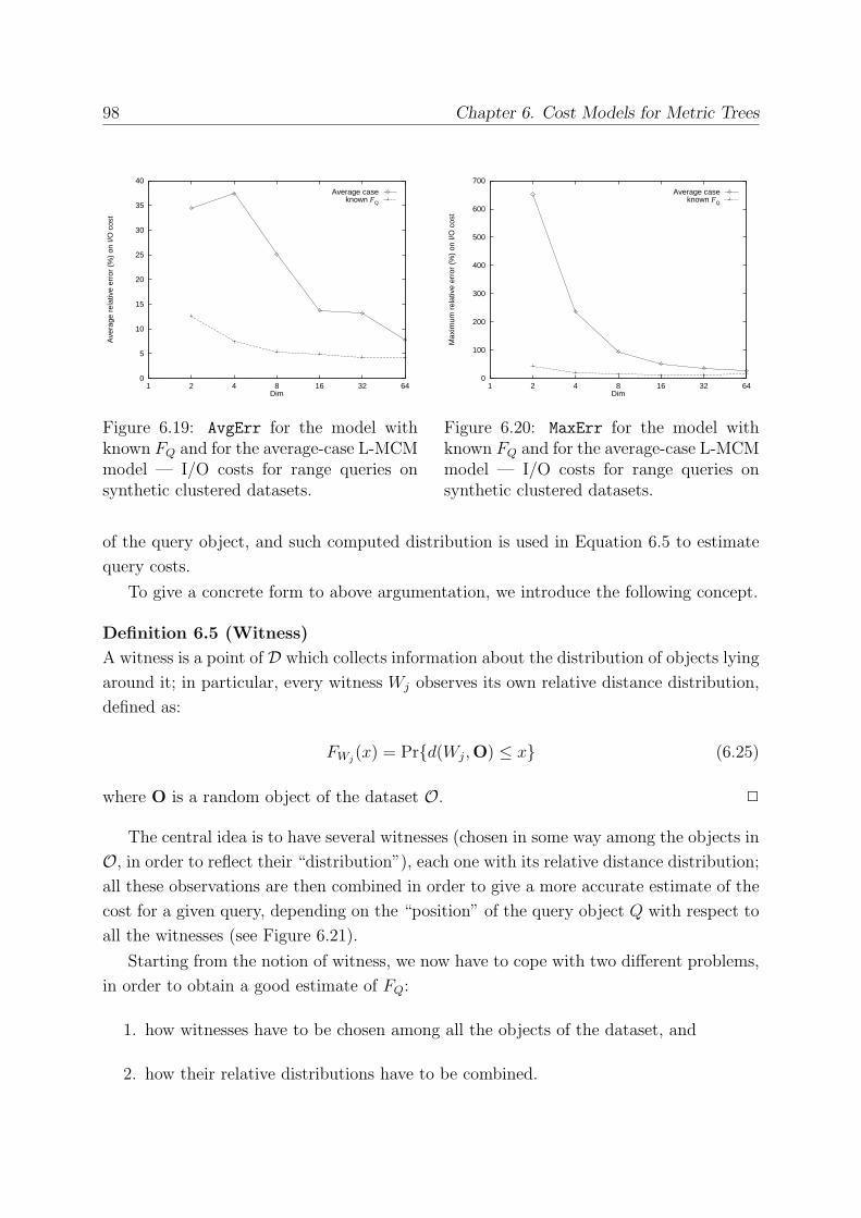
98 Chapter 6. Cost Models for Metric Trees
0
5
10
15
20
25
30
35
40
1 2 4 8 16 32 64
Ave
rage
rel
ativ
e er
ror
(%)
on I/
O c
ost
Dim
Average caseknown FQ
Figure 6.19: AvgErr for the model withknown FQ and for the average-case L-MCMmodel — I/O costs for range queries onsynthetic clustered datasets.
0
100
200
300
400
500
600
700
1 2 4 8 16 32 64
Max
imum
rel
ativ
e er
ror
(%)
on I/
O c
ost
Dim
Average caseknown FQ
Figure 6.20: MaxErr for the model withknown FQ and for the average-case L-MCMmodel — I/O costs for range queries onsynthetic clustered datasets.
of the query object, and such computed distribution is used in Equation 6.5 to estimate
query costs.
To give a concrete form to above argumentation, we introduce the following concept.
Definition 6.5 (Witness)
A witness is a point of D which collects information about the distribution of objects lyingaround it; in particular, every witness Wj observes its own relative distance distribution,
defined as:
FWj(x) = Pr{d(Wj,O) ≤ x} (6.25)
where O is a random object of the dataset O. ✷
The central idea is to have several witnesses (chosen in some way among the objects in
O, in order to reflect their “distribution”), each one with its relative distance distribution;all these observations are then combined in order to give a more accurate estimate of the
cost for a given query, depending on the “position” of the query object Q with respect to
all the witnesses (see Figure 6.21).
Starting from the notion of witness, we now have to cope with two different problems,
in order to obtain a good estimate of FQ:
1. how witnesses have to be chosen among all the objects of the dataset, and
2. how their relative distributions have to be combined.
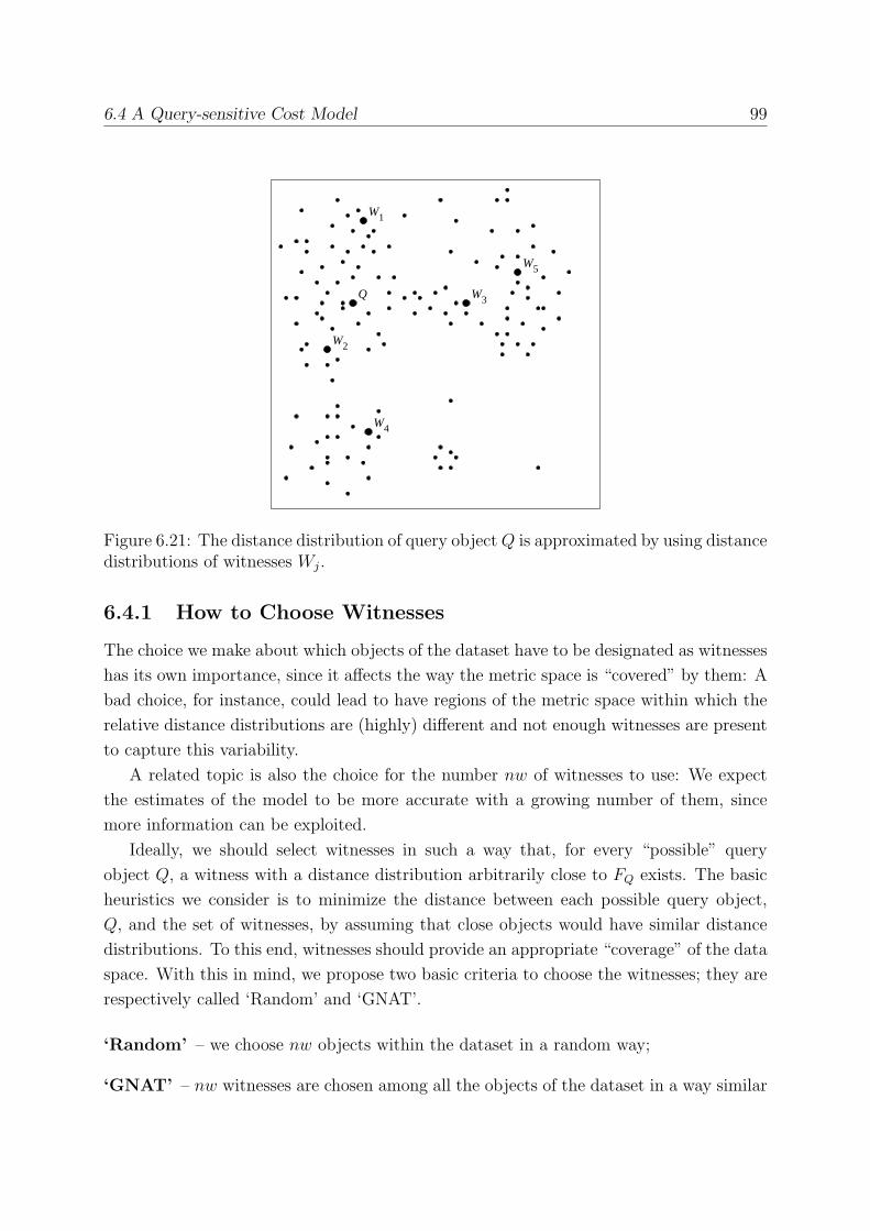
6.4 A Query-sensitive Cost Model 99
W1
Q
W2
W4
W3
W5
Figure 6.21: The distance distribution of query objectQ is approximated by using distancedistributions of witnesses Wj.
6.4.1 How to Choose Witnesses
The choice we make about which objects of the dataset have to be designated as witnesses
has its own importance, since it affects the way the metric space is “covered” by them: A
bad choice, for instance, could lead to have regions of the metric space within which the
relative distance distributions are (highly) different and not enough witnesses are present
to capture this variability.
A related topic is also the choice for the number nw of witnesses to use: We expect
the estimates of the model to be more accurate with a growing number of them, since
more information can be exploited.
Ideally, we should select witnesses in such a way that, for every “possible” query
object Q, a witness with a distance distribution arbitrarily close to FQ exists. The basic
heuristics we consider is to minimize the distance between each possible query object,
Q, and the set of witnesses, by assuming that close objects would have similar distance
distributions. To this end, witnesses should provide an appropriate “coverage” of the data
space. With this in mind, we propose two basic criteria to choose the witnesses; they are
respectively called ‘Random’ and ‘GNAT’.
‘Random’ – we choose nw objects within the dataset in a random way;
‘GNAT’ – nw witnesses are chosen among all the objects of the dataset in a way similar
100 Chapter 6. Cost Models for Metric Trees
to the one used in the GNAT access method [Bri95] to designate “split points”.
In practice, the ‘GNAT’ method first extracts from the dataset a random sample
of 3 · nw objects, called candidate objects; then, within this sample, nw witnesses
are chosen far apart each other. More specifically, this is done as follows: A first
witness is picked at random within the set of candidate objects; then we choose the
candidate point which is farthest away from this one; then we pick the candidate
point which is the farthest from these two (that is, its minimum distance from the
two is maximized), and so on.
Of course the ‘Random’ method has the advantage of being much easier and faster;
moreover, since witnesses are distributed like objects in O, it is very likely that eachquery object will have a “near” witness, under the assumption of a biased query model,
i.e. indexed and query objects follow the same distribution (see also Section 6.2). On
the other hand, the ‘GNAT’ method has the purpose to “cover” the region of the metric
space relative to the dataset in a somewhat homogeneous way, avoiding the “crowding”
of witnesses in dense regions of the space; in this way, we try to minimize the maximum
possible distance between a query object and its nearest witness.
6.4.2 How to Combine Relative Distance Distributions
Starting from the relative distance distributions observed by several witnesses, the next
problem consists in how to combine this information in order to give a proper estimate of
FQ. Again, the basic rationale is that close objects have similar distance distributions.
We consider two main criteria to cope with this problem; moreover, we also propose
a specific variant for the second one.
‘Nearest Witness’ Method
This method estimates FQ as follows:
FQ(x) % FWNW(x) with d(WNW , Q) ≤ d(Wj, Q), j = 1, . . . , nw (6.26)
that is, the unknown distribution relative to the query object Q is approximated with
the one relative to its nearest witness. This method is quite easy to use, since it only
requires to estabilish which is the nearest witness and no new distance distribution has
to be computed.
6.4 A Query-sensitive Cost Model 101
‘Distance Weighted’ Method
This method estimates FQ as follows:
FQ(x) %∑nw
j=1 Fj(x) · αj∑nwj=1 αj
(6.27)
In other terms, FQ is estimated as a weighted average of all the relative distance
distributions observed by the witnesses, with generic weights αj. Of course, different
choices for the weights lead to different performance for the model. Our assumption,
however, is that witnesses closer to Q are supposed to be more “reliable”, since their
distance distribution is more similar to that of the query object itself. Therefore, weights
αj in Equation 6.27 should be inversely related to the distance between the query object
Q and the witnesses Wj. Our choice is to use the Exp-th power of the inverse of the
distance between a witness and Q, that is:
αj = d(Wj, Q)−Exp (6.28)
We point out that the ‘Nearest Witness’ method is the limit of the ‘Distance Weighted’
method when Exp goes to infinity. On the other end, for Exp = 0 we obtain the classic
arithmetic average, which means that we equally weigh the contribution given by each
witness.
‘Distance Weighted’, Adaptive Method
The ‘Distance Weighted’ method is dependent on the parameter Exp, so different choices
for the value of the exponent lead to different results (as we will see in Section 6.4.3).
It would be, therefore, desirable to find a way to dynamically compute a “proper” value
for Exp. Here we propose an adaptive variant of the ‘Distance Weighted’ method which
computes a value for Exp as a function of the query object at hand.
The basic idea of this method is to choose a value for Exp as a function of the distances
between witnesses and the query object. When, on the average, these distances are all
somewhat “high”, it does not make sense relying on the nearest witness, so we choose a
low value for Exp. On the other hand, when, on the average, witnesses are very close to
Q, we can rely more on the nearest witness, thus choosing a high value for Exp.
We define the average distance of witnesses from Q, normalized to maximum distance
d+, as follows:
mdw =nw∑j=1
d(Wj, Q)
d+ · nw (6.29)
102 Chapter 6. Cost Models for Metric Trees
Now, for a given query, Exp can be computed as:
Exp = (1−mdw) ·MaxExp (6.30)
where MaxExp has to be thought as that value of Exp for which the two methods,
‘Distance Weighted’ and ‘Nearest Witness’, give very similar estimates. Experimentally
we found out that an acceptable value is MaxExp = 10; this is also the value adopted in
all the tests we carried out.
6.4.3 Experimental Evaluation
In order to evaluate the accuracy of our cost models, we ran several experiments on
both synthetic and real datasets (see Table 6.2). Estimates are compared with actual
results obtained by the M-tree, which, again, was built using the BulkLoading algorithm
described in Chapter 5 with a node size of 4 Kbytes and a minimum node utilization of
30%.
For each test we ran, 500 similarity queries were executed; unless otherwise stated, for
range queries we used a radius rQ =D√0.01/2 for synthetic datasets and a radius rQ = 3
for real datasets. For k-nearest neighbor queries we considered only k = 1, which is the
most common case.
For each distance distribution needed in the experiments we ran, an estimate of its
density function f was obtained from an analysis of the dataset O. In particular, for theoverall distance distribution we sampled all the n(n− 1)/2 pairwise distances between allthe n objects of O; for each distance distribution relative to a single witness we consideredall the n− 1 distances between this witness and any other object of O.
In both cases, starting from this sample we built a 100 bins equi-width histogram
of type ASH (Averaged Shifted Histogram, as described in [Sco92]) which represents an
approximation of the density function f .
6.4.4 Experimental Results
In this Section we present some results showing the performance of our query-sensitive
cost model; we also compare its different methods with the previous average-case cost
model. The reported graphs, to keep it short, only refer to I/O costs, since errors on
estimates of CPU costs show a very similar trend.
First of all, in Figures 6.22 and 6.23 we present some results concerning the incidence
on estimates of how witnesses are chosen and of their number, respectively. For simplicity,
we consider only the values of AvgErr for the ‘Nearest Witness’ method relative to range
queries on synthetic clustered datasets.
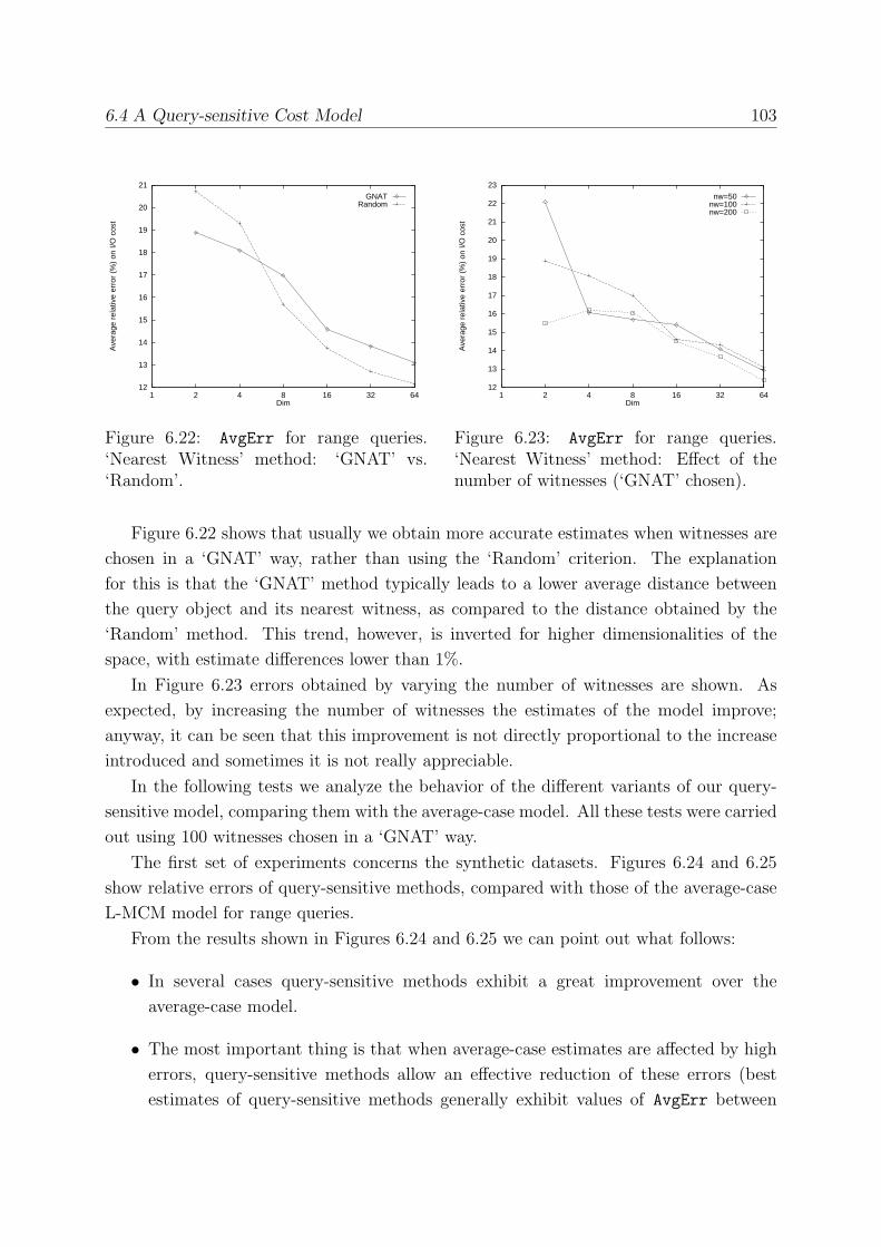
6.4 A Query-sensitive Cost Model 103
12
13
14
15
16
17
18
19
20
21
1 2 4 8 16 32 64
Ave
rage
rel
ativ
e er
ror
(%)
on I/
O c
ost
Dim
GNATRandom
Figure 6.22: AvgErr for range queries.‘Nearest Witness’ method: ‘GNAT’ vs.‘Random’.
12
13
14
15
16
17
18
19
20
21
22
23
1 2 4 8 16 32 64
Ave
rage
rel
ativ
e er
ror
(%)
on I/
O c
ost
Dim
nw=50nw=100nw=200
Figure 6.23: AvgErr for range queries.‘Nearest Witness’ method: Effect of thenumber of witnesses (‘GNAT’ chosen).
Figure 6.22 shows that usually we obtain more accurate estimates when witnesses are
chosen in a ‘GNAT’ way, rather than using the ‘Random’ criterion. The explanation
for this is that the ‘GNAT’ method typically leads to a lower average distance between
the query object and its nearest witness, as compared to the distance obtained by the
‘Random’ method. This trend, however, is inverted for higher dimensionalities of the
space, with estimate differences lower than 1%.
In Figure 6.23 errors obtained by varying the number of witnesses are shown. As
expected, by increasing the number of witnesses the estimates of the model improve;
anyway, it can be seen that this improvement is not directly proportional to the increase
introduced and sometimes it is not really appreciable.
In the following tests we analyze the behavior of the different variants of our query-
sensitive model, comparing them with the average-case model. All these tests were carried
out using 100 witnesses chosen in a ‘GNAT’ way.
The first set of experiments concerns the synthetic datasets. Figures 6.24 and 6.25
show relative errors of query-sensitive methods, compared with those of the average-case
L-MCM model for range queries.
From the results shown in Figures 6.24 and 6.25 we can point out what follows:
• In several cases query-sensitive methods exhibit a great improvement over theaverage-case model.
• The most important thing is that when average-case estimates are affected by higherrors, query-sensitive methods allow an effective reduction of these errors (best
estimates of query-sensitive methods generally exhibit values of AvgErr between
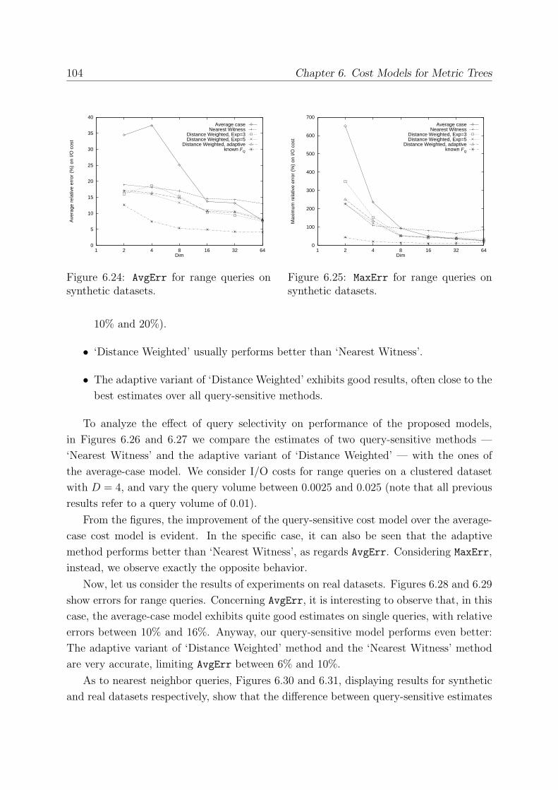
104 Chapter 6. Cost Models for Metric Trees
0
5
10
15
20
25
30
35
40
1 2 4 8 16 32 64
Ave
rage
rel
ativ
e er
ror
(%)
on I/
O c
ost
Dim
Average caseNearest Witness
Distance Weighted, Exp=3Distance Weighted, Exp=5
Distance Weighted, adaptiveknown FQ
Figure 6.24: AvgErr for range queries onsynthetic datasets.
0
100
200
300
400
500
600
700
1 2 4 8 16 32 64
Max
imum
rel
ativ
e er
ror
(%)
on I/
O c
ost
Dim
Average caseNearest Witness
Distance Weighted, Exp=3Distance Weighted, Exp=5
Distance Weighted, adaptiveknown FQ
Figure 6.25: MaxErr for range queries onsynthetic datasets.
10% and 20%).
• ‘Distance Weighted’ usually performs better than ‘Nearest Witness’.
• The adaptive variant of ‘Distance Weighted’ exhibits good results, often close to thebest estimates over all query-sensitive methods.
To analyze the effect of query selectivity on performance of the proposed models,
in Figures 6.26 and 6.27 we compare the estimates of two query-sensitive methods —
‘Nearest Witness’ and the adaptive variant of ‘Distance Weighted’ — with the ones of
the average-case model. We consider I/O costs for range queries on a clustered dataset
with D = 4, and vary the query volume between 0.0025 and 0.025 (note that all previous
results refer to a query volume of 0.01).
From the figures, the improvement of the query-sensitive cost model over the average-
case cost model is evident. In the specific case, it can also be seen that the adaptive
method performs better than ‘Nearest Witness’, as regards AvgErr. Considering MaxErr,
instead, we observe exactly the opposite behavior.
Now, let us consider the results of experiments on real datasets. Figures 6.28 and 6.29
show errors for range queries. Concerning AvgErr, it is interesting to observe that, in this
case, the average-case model exhibits quite good estimates on single queries, with relative
errors between 10% and 16%. Anyway, our query-sensitive model performs even better:
The adaptive variant of ‘Distance Weighted’ method and the ‘Nearest Witness’ method
are very accurate, limiting AvgErr between 6% and 10%.
As to nearest neighbor queries, Figures 6.30 and 6.31, displaying results for synthetic
and real datasets respectively, show that the difference between query-sensitive estimates
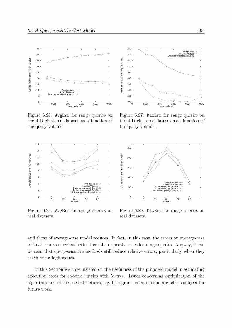
6.4 A Query-sensitive Cost Model 105
0
5
10
15
20
25
30
35
40
45
0 0.005 0.01 0.015 0.02 0.025
Ave
rage
rel
ativ
e er
ror
(%)
on I/
O c
ost
query volume
Average-caseNearest Witness
Distance Weighted, adaptive
Figure 6.26: AvgErr for range queries onthe 4-D clustered dataset as a function ofthe query volume.
100
120
140
160
180
200
220
240
260
280
0 0.005 0.01 0.015 0.02 0.025
Max
imum
rel
ativ
e er
ror
(%)
on I/
O c
ost
query volume
Average-caseNearest Witness
Distance Weighted, adaptive
Figure 6.27: MaxErr for range queries onthe 4-D clustered dataset as a function ofthe query volume.
0
2
4
6
8
10
12
14
16
D DC GL OF PS
Ave
rage
rel
ativ
e er
ror
(%)
on I/
O c
ost
dataset
Average-caseNearest Witness
Distance Weighted, Exp=3Distance Weighted, Exp=5
Distance Weighted, adaptive
Figure 6.28: AvgErr for range queries onreal datasets.
0
50
100
150
200
250
D DC GL OF PS
Max
imum
rel
ativ
e er
ror
(%)
on I/
O c
ost
dataset
Average-caseNearest Witness
Distance Weighted, Exp=3Distance Weighted, Exp=5
Distance Weighted, adaptive
Figure 6.29: MaxErr for range queries onreal datasets.
and those of average-case model reduces. In fact, in this case, the errors on average-case
estimates are somewhat better than the respective ones for range queries. Anyway, it can
be seen that query-sensitive methods still reduce relative errors, particularly when they
reach fairly high values.
In this Section we have insisted on the usefulness of the proposed model in estimating
execution costs for specific queries with M-tree. Issues concerning optimization of the
algorithm and of the used structures, e.g. histograms compression, are left as subject for
future work.
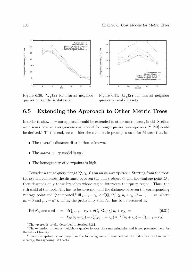
106 Chapter 6. Cost Models for Metric Trees
0
5
10
15
20
25
30
35
1 2 4 8 16 32 64
Ave
rage
rel
ativ
e er
ror
(%)
on I/
O c
ost
Dim
Average-caseNearest Witness
Distance Weighted, Exp=3Distance Weighted, Exp=5
Distance Weighted, adaptive
Figure 6.30: AvgErr for nearest neighborqueries on synthetic datasets.
0
10
20
30
40
50
D DC GL OF PS
Ave
rage
rel
ativ
e er
ror
(%)
on I/
O c
ost
dataset
Average-caseNearest Witness
Distance Weighted, Exp=3Distance Weighted, Exp=5
Distance Weighted, adaptive
Figure 6.31: AvgErr for nearest neighborqueries on real datasets.
6.5 Extending the Approach to Other Metric Trees
In order to show how our approach could be extended to other metric trees, in this Section
we discuss how an average-case cost model for range queries over vp-trees [Yia93] could
be derived.4 To this end, we consider the same basic principles used for M-tree, that is:
• The (overall) distance distribution is known.
• The biased query model is used.
• The homogeneity of viewpoints is high.
Consider a range query range(Q, rQ, C) on an m-way vp-tree.5 Starting from the root,the system computes the distance between the query object Q and the vantage point Ov,
then descends only those branches whose region intersects the query region. Thus, the
i-th child of the root, Nri, has to be accessed, and the distance between the corresponding
vantage point and Q computed,6 iff µi−1− rQ < d(Q,Ov) ≤ µi+ rQ, (i = 1, . . . ,m, where
µ0 = 0 and µm = d+). Thus, the probability that Nrihas to be accessed is:
Pr{Nriaccessed} = Pr{µi−1 − rQ < d(Q,Ov) ≤ µi + rQ} = (6.31)
= FQ(µi + rQ)− FQ(µi−1 − rQ) ≈ F (µi + rQ)− F (µi−1 − rQ)
4The vp-tree is briefly described in Section 3.2.1.5The extension to nearest neighbors queries follows the same principles and is not presented here for
the sake of brevity.6Since the vp-tree is not paged, in the following we will assume that the index is stored in main
memory, thus ignoring I/O costs.
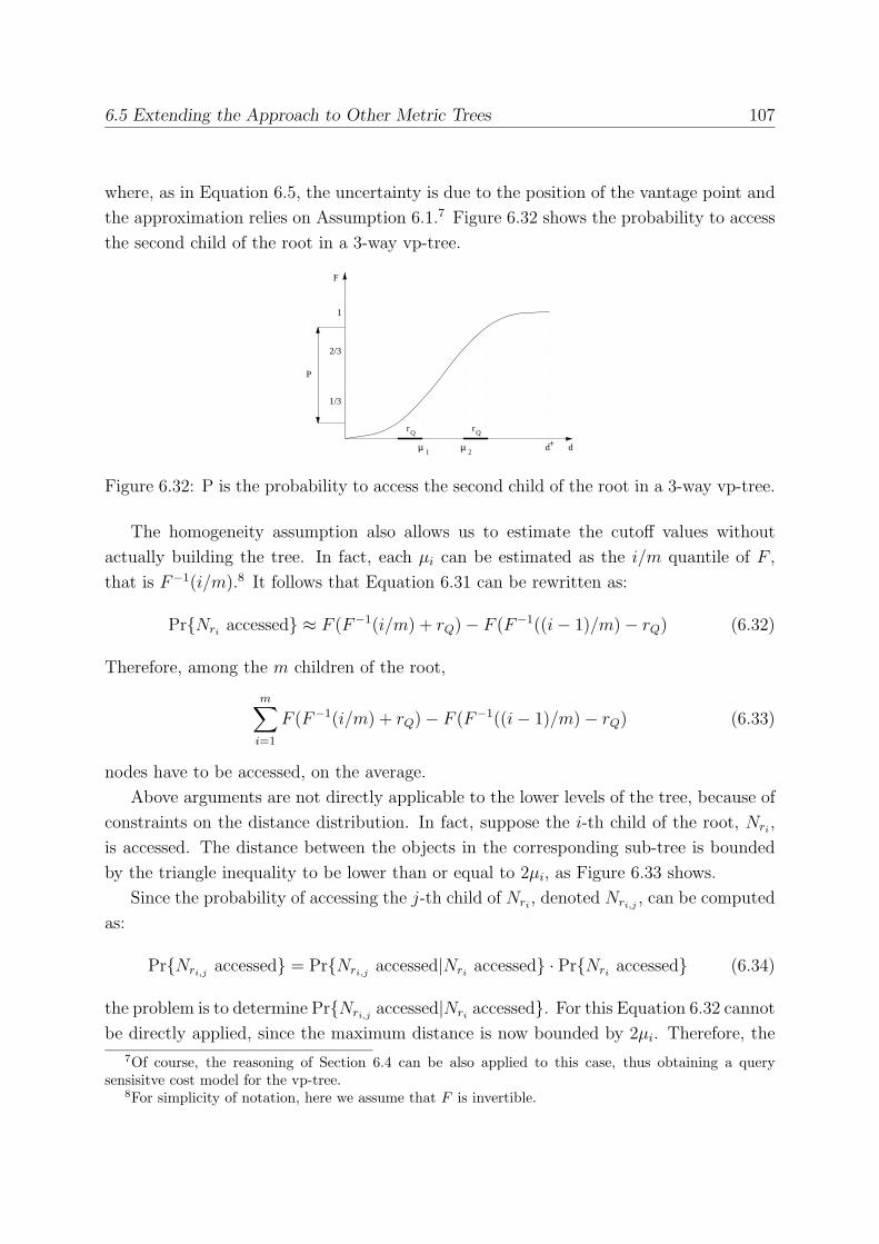
6.5 Extending the Approach to Other Metric Trees 107
where, as in Equation 6.5, the uncertainty is due to the position of the vantage point and
the approximation relies on Assumption 6.1.7 Figure 6.32 shows the probability to access
the second child of the root in a 3-way vp-tree.
µ 1 µ 2
rQ rQ
d+
1
2/3
1/3
P
F
d
Figure 6.32: P is the probability to access the second child of the root in a 3-way vp-tree.
The homogeneity assumption also allows us to estimate the cutoff values without
actually building the tree. In fact, each µi can be estimated as the i/m quantile of F ,
that is F−1(i/m).8 It follows that Equation 6.31 can be rewritten as:
Pr{Nriaccessed} ≈ F (F−1(i/m) + rQ)− F (F−1((i− 1)/m)− rQ) (6.32)
Therefore, among the m children of the root,
m∑i=1
F (F−1(i/m) + rQ)− F (F−1((i− 1)/m)− rQ) (6.33)
nodes have to be accessed, on the average.
Above arguments are not directly applicable to the lower levels of the tree, because of
constraints on the distance distribution. In fact, suppose the i-th child of the root, Nri,
is accessed. The distance between the objects in the corresponding sub-tree is bounded
by the triangle inequality to be lower than or equal to 2µi, as Figure 6.33 shows.
Since the probability of accessing the j-th child of Nri, denoted Nri,j
, can be computed
as:
Pr{Nri,jaccessed} = Pr{Nri,j
accessed|Nriaccessed} · Pr{Nri
accessed} (6.34)
the problem is to determine Pr{Nri,jaccessed|Nri
accessed}. For this Equation 6.32 cannotbe directly applied, since the maximum distance is now bounded by 2µi. Therefore, the
7Of course, the reasoning of Section 6.4 can be also applied to this case, thus obtaining a querysensisitve cost model for the vp-tree.
8For simplicity of notation, here we assume that F is invertible.
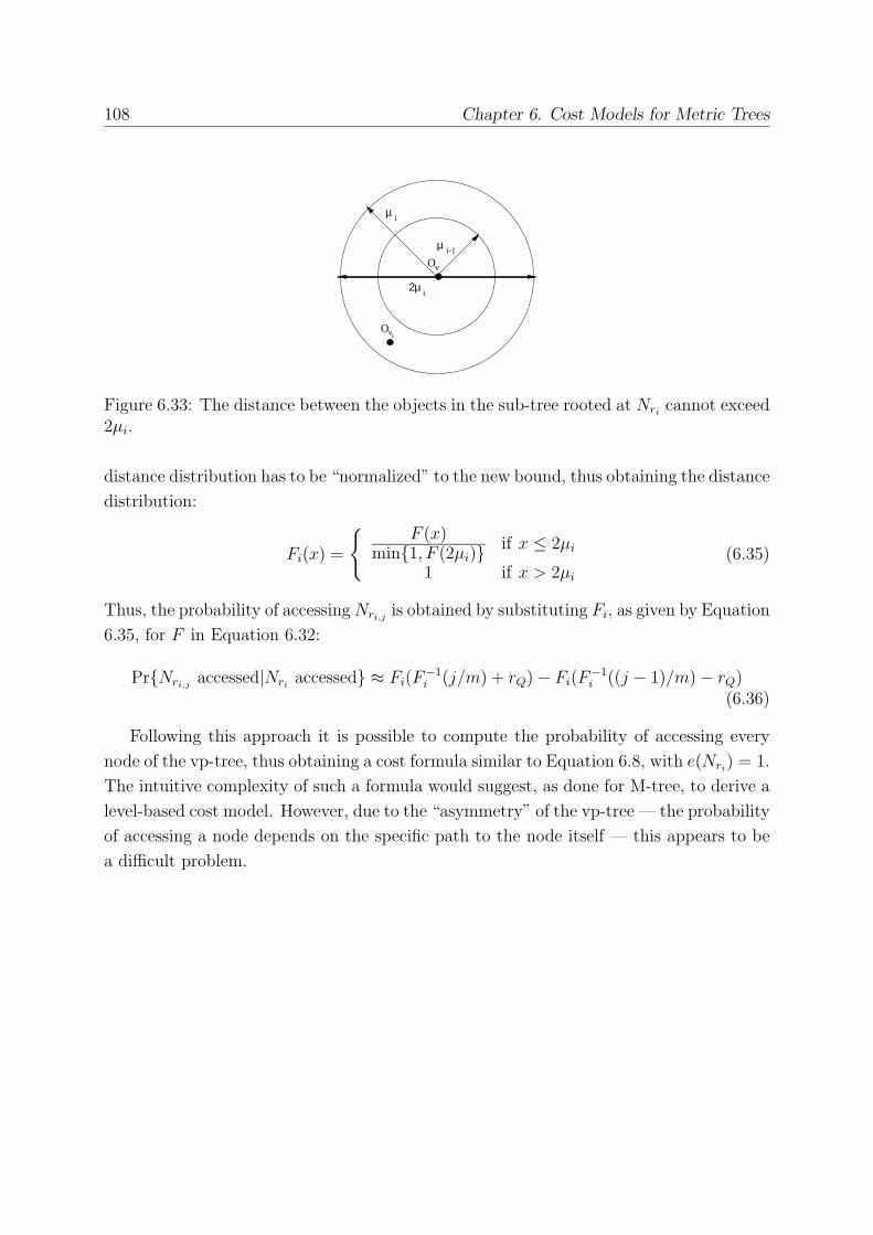
108 Chapter 6. Cost Models for Metric Trees
µ i-1
µ i
2µ i
Ov
vOi
Figure 6.33: The distance between the objects in the sub-tree rooted at Nricannot exceed
2µi.
distance distribution has to be “normalized” to the new bound, thus obtaining the distance
distribution:
Fi(x) =
{F (x)
min{1, F (2µi)} if x ≤ 2µi1 if x > 2µi
(6.35)
Thus, the probability of accessingNri,jis obtained by substituting Fi, as given by Equation
6.35, for F in Equation 6.32:
Pr{Nri,jaccessed|Nri
accessed} ≈ Fi(F−1i (j/m) + rQ)− Fi(F
−1i ((j − 1)/m)− rQ)
(6.36)
Following this approach it is possible to compute the probability of accessing every
node of the vp-tree, thus obtaining a cost formula similar to Equation 6.8, with e(Nri) = 1.
The intuitive complexity of such a formula would suggest, as done for M-tree, to derive a
level-based cost model. However, due to the “asymmetry” of the vp-tree — the probability
of accessing a node depends on the specific path to the node itself — this appears to be
a difficult problem.
Chapter 7
Complex Queries
In Chapter 2, we showed how simple similarity queries can be transformed, by means
of a correspondence function h, into distance-based queries. Then, in Chapters 3 and 4,
we saw how such simple distance queries can be efficiently evaluated with distance-based
access methods (SAMs and metric trees).
In this Chapter, we consider the relevant case where complex similarity queries —
queries consisting of more than one similarity predicate — are defined. The problem of
efficiently processing complex similarity queries has been highlighted only by recent works
[CG96, Fag96, FW97]. The basic lesson is that, since the “similarity score” (grade) an
object gets for the whole query depends on how the scores it gets for the single predicates
are combined, predicates cannot be independently evaluated.
Example 7.1
Consider an image database where objects can be retrieved by means of predicates on
shape and color features, and assume that the two sets of feature values are separately
indexed. In order to retrieve the best match for the query
(shape = ‘circular’) and (color = ‘red’)
it is not correct to retrieve only the best match for color (using an index on color) and
the best match for shape (using an index on shape), since the best match for the overall
query needs not to be the best match for the single conjuncts. ✷
In this Chapter we first concentrate on a relevant class of complex similarity queries,
which arises when all the similarity predicates refer to a single feature, then, in Section
7.5, we will extend our approach to the general multi-feature case. It is important to note
that single-feature queries are an interesting subset of generic complex queries [CPZ98b].
Example 7.2
Consider an image database where objects can be retrieved using a Query-by-Sketch
109
110 Chapter 7. Complex Queries
modality (see also Example 2.1). When a user draws a shape on the screen, the system
searches the DB, and returns those, say, 10 images which contain a shape best matching
(according to given similarity criterion for shapes) the user’s input. The user can then
“refine” the search by selecting those objects which are similar to what he/she had in
mind and which are actually not. Suppose two “positive” and one “negative” samples
are specified. Now, the system has to search the DB for those 10 objects which are most
similar to both positive samples, and, at the same time, not similar to the negative one.
This interactive process can be iterated several times, until the user gets satisfied with
system’s output. ✷
An interactive retrieval process, such as the one sketched above, typically occurs when
querying multimedia repositories [Jai96], where the user has no clear idea on how to ex-
press what he/she is looking for, and relies on previous results to improve the effectiveness
of subsequent requests.1
7.1 The Problem
In Section 2.1 we introduced the basic ingredients to deal with simple similarity queries,
i.e. the concepts of feature, similarity predicate, and similarity score. Since, now, our
objective is to deal with complex similarity queries, we need a language L which allowsmultiple predicates to be combined into a similarity formula, f . The nature of the specific
language is uninfluential to our arguments. We only require the existence of a scoring
function [Fag96] computing the overall score of an object with respect to the complex
similarity formula f , considering all the scores of the object itself with respect to the
predicates of f .
Definition 7.1 (Scoring function)
If f = f(p1, . . . , pn) is a formula of L, then the similarity of an object O with respect
to f , denoted s(f,O), is computed through a corresponding scoring function, sf , which
takes as input the scores of O with respect to the predicates of formula f , that is:
s(f(p1, . . . , pn), O) = sf (s(p1, O), . . . , s(pn, O)) (7.1)
✷
Shortly, we will introduce three specific sample languages to construct similarity for-
mulae. For the moment, we provide the following definitions which exactly specify the
kinds of queries we are going to deal with.1Although some connections with the relevance feedback techniques applied to textual document re-
trieval [Har92] can be observed, the scenario we envision has a broader context.
7.1 The Problem 111
Definition 7.2 (Complex range query)
Given a similarity formula f ∈ L and a minimum similarity threshold α, the query
range(f, α, C) selects all the objects in C (with their scores) such that s(f,O) ≥ α, that
is, objects whose overall score with respect to f , as determined by the language L, is notless than α. ✷
Definition 7.3 (Complex nearest neighbors (k-NN) query)
Given a similarity formula f and an integer k ≥ 1, the k-NN query NN(f, k, C) selects thek objects in C having the highest similarity scores with respect to f . In case of ties, theyare arbitrarily broken. ✷
7.1.1 Similarity Languages
A similarity language L comes with a syntax, specifying which are valid (well-formed)formulae, and a semantics, telling us how to evaluate the similarity of an object with
respect to a complex query. Although the results we present are language-independent,
it also helps intuition to consider specific examples.
The first two languages we consider, FS (fuzzy standard) and FA (fuzzy algebraic),
share the same syntax and stay in the framework of fuzzy logic [Zad65, KY95]. The third
language, WS (weighted sum), does not use logical connectives at all, but allows weightsto be attached to the predicates, in order to reflect the importance the user wants to
assign to each of them.
The language FS
The language FS is based on the “standard” semantics of fuzzy logic [Zad65]. Formulaeof FS are defined by the following grammar rule:
f ::= p|f ∧ f |f ∨ f |¬f |(f) (7.2)
where p is a similarity predicate. The semantics of a formula f is given by the following
set of recursive rules:
s(f1 ∧ f2, O) = min{s(f1, O), s(f2, O)}s(f1 ∨ f2, O) = max{s(f1, O), s(f2, O)}
s(¬f,O) = 1− s(f,O)
112 Chapter 7. Complex Queries
The language FA
The language FA has the same syntax as FS, as defined in Equation 7.2, but it uses an“algebraic” semantics for logical operators [KY95], which are defined as follows:
s(f1 ∧ f2, O) = s(f1, O) · s(f2, O)
s(f1 ∨ f2, O) = s(f1, O) + s(f2, O)− s(f1, O) · s(f2, O)
s(¬f,O) = 1− s(f,O)
The language WS
The last language we consider,WS, aims to show the generality of the presented approach,and is based on the well-known model of “list-of-keywords”. A formula f has the form:
f ::= {(p1, θ1), (p2, θ2), . . . , (pn, θn)}
where each pi is a similarity predicate, the θi’s are positive weights, and∑n
i=1 θi = 1. The
semantics of a WS formula f is simply:
s(f,O) =n∑i=1
θi · s(pi, O)
Although the subject of deciding on which is the “best” language is not in the scope
of this work, it is important to realize that any specific language has some advantages
and drawbacks, thus making the choice a difficult problem. For instance, it is known
that if two negation-free formulae f1 and f2 are equivalent under Boolean semantics, then
they are also equivalent according to FS, which is clearly a desirable property from the
optimization point of view. As an example, p1 ∨ p1 ∧ p2 = p1 is a correct equivalence in
FS. On the other hand, it is not correct under FA semantics, as it can be easily shown.On the other side, FS is single-operand dependent, meaning that s(f1 ∧ f2, O) (as well as
s(f1 ∨ f2, O)) is always equal either to s(f1, O) or to s(f2, O). This suggests that FS isnot the best choice if one wants the final score an object obtains to be a “combination”
of the scores of all the predicates.
We also remark that above languages are only a selected sample of the many one can
conceive to formulate complex queries, and that our approach is not limited only to them.
In particular, our results also apply to fuzzy languages, such as FS and FA, when theyare extended with weights, as shown in [FW97].
Example 7.3
Assume that we want to retrieve objects which are similar to both query values v1 and v2.
With the FS and FA languages we can use the formula f1 = p1 ∧ p2, where pi : F ∼ vi.
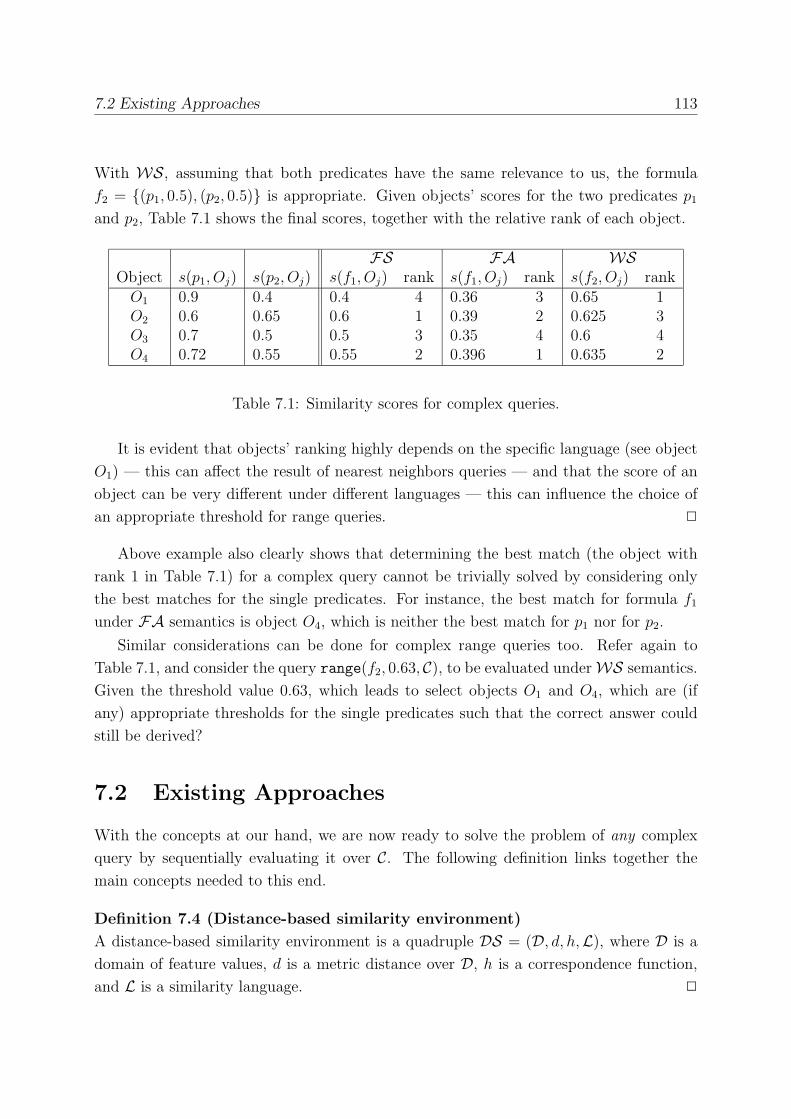
7.2 Existing Approaches 113
With WS, assuming that both predicates have the same relevance to us, the formulaf2 = {(p1, 0.5), (p2, 0.5)} is appropriate. Given objects’ scores for the two predicates p1
and p2, Table 7.1 shows the final scores, together with the relative rank of each object.
FS FA WSObject s(p1, Oj) s(p2, Oj) s(f1, Oj) rank s(f1, Oj) rank s(f2, Oj) rankO1 0.9 0.4 0.4 4 0.36 3 0.65 1O2 0.6 0.65 0.6 1 0.39 2 0.625 3O3 0.7 0.5 0.5 3 0.35 4 0.6 4O4 0.72 0.55 0.55 2 0.396 1 0.635 2
Table 7.1: Similarity scores for complex queries.
It is evident that objects’ ranking highly depends on the specific language (see object
O1) — this can affect the result of nearest neighbors queries — and that the score of an
object can be very different under different languages — this can influence the choice of
an appropriate threshold for range queries. ✷
Above example also clearly shows that determining the best match (the object with
rank 1 in Table 7.1) for a complex query cannot be trivially solved by considering only
the best matches for the single predicates. For instance, the best match for formula f1
under FA semantics is object O4, which is neither the best match for p1 nor for p2.
Similar considerations can be done for complex range queries too. Refer again to
Table 7.1, and consider the query range(f2, 0.63, C), to be evaluated underWS semantics.Given the threshold value 0.63, which leads to select objects O1 and O4, which are (if
any) appropriate thresholds for the single predicates such that the correct answer could
still be derived?
7.2 Existing Approaches
With the concepts at our hand, we are now ready to solve the problem of any complex
query by sequentially evaluating it over C. The following definition links together themain concepts needed to this end.
Definition 7.4 (Distance-based similarity environment)
A distance-based similarity environment is a quadruple DS = (D, d, h,L), where D is a
domain of feature values, d is a metric distance over D, h is a correspondence function,and L is a similarity language. ✷
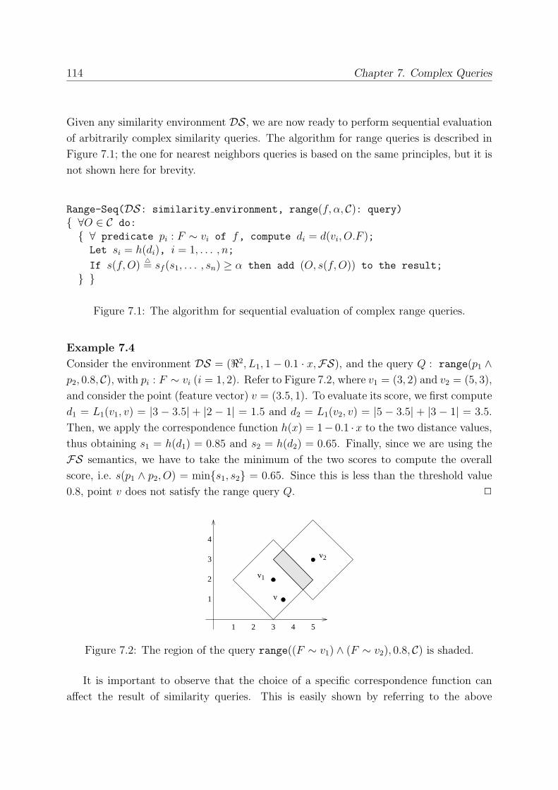
114 Chapter 7. Complex Queries
Given any similarity environment DS, we are now ready to perform sequential evaluation
of arbitrarily complex similarity queries. The algorithm for range queries is described in
Figure 7.1; the one for nearest neighbors queries is based on the same principles, but it is
not shown here for brevity.
Range-Seq(DS: similarity environment, range(f, α, C): query)
{ ∀O ∈ C do:
{ ∀ predicate pi : F ∼ vi of f, compute di = d(vi, O.F );Let si = h(di), i = 1, . . . , n;
If s(f,O)�= sf (s1, . . . , sn) ≥ α then add (O, s(f,O)) to the result;
} }
Figure 7.1: The algorithm for sequential evaluation of complex range queries.
Example 7.4
Consider the environment DS = (�2, L1, 1− 0.1 · x,FS), and the query Q : range(p1 ∧p2, 0.8, C), with pi : F ∼ vi (i = 1, 2). Refer to Figure 7.2, where v1 = (3, 2) and v2 = (5, 3),
and consider the point (feature vector) v = (3.5, 1). To evaluate its score, we first compute
d1 = L1(v1, v) = |3 − 3.5| + |2 − 1| = 1.5 and d2 = L1(v2, v) = |5 − 3.5| + |3 − 1| = 3.5.Then, we apply the correspondence function h(x) = 1− 0.1 ·x to the two distance values,thus obtaining s1 = h(d1) = 0.85 and s2 = h(d2) = 0.65. Finally, since we are using the
FS semantics, we have to take the minimum of the two scores to compute the overall
score, i.e. s(p1 ∧ p2, O) = min{s1, s2} = 0.65. Since this is less than the threshold value0.8, point v does not satisfy the range query Q. ✷
1 2 3 4 5
v1
v2
2
3
4
1 v
Figure 7.2: The region of the query range((F ∼ v1) ∧ (F ∼ v2), 0.8, C) is shaded.
It is important to observe that the choice of a specific correspondence function can
affect the result of similarity queries. This is easily shown by referring to the above
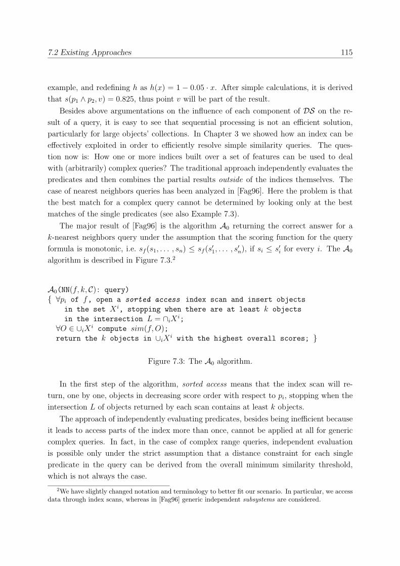
7.2 Existing Approaches 115
example, and redefining h as h(x) = 1 − 0.05 · x. After simple calculations, it is derivedthat s(p1 ∧ p2, v) = 0.825, thus point v will be part of the result.
Besides above argumentations on the influence of each component of DS on the re-sult of a query, it is easy to see that sequential processing is not an efficient solution,
particularly for large objects’ collections. In Chapter 3 we showed how an index can be
effectively exploited in order to efficiently resolve simple similarity queries. The ques-
tion now is: How one or more indices built over a set of features can be used to deal
with (arbitrarily) complex queries? The traditional approach independently evaluates the
predicates and then combines the partial results outside of the indices themselves. The
case of nearest neighbors queries has been analyzed in [Fag96]. Here the problem is that
the best match for a complex query cannot be determined by looking only at the best
matches of the single predicates (see also Example 7.3).
The major result of [Fag96] is the algorithm A0 returning the correct answer for a
k-nearest neighbors query under the assumption that the scoring function for the query
formula is monotonic, i.e. sf (s1, . . . , sn) ≤ sf (s′1, . . . , s
′n), if si ≤ s′i for every i. The A0
algorithm is described in Figure 7.3.2
A0(NN(f, k, C): query)
{ ∀pi of f, open a sorted access index scan and insert objects
in the set X i, stopping when there are at least k objects
in the intersection L = ∩iXi;
∀O ∈ ∪iXi compute sim(f,O);
return the k objects in ∪iXi with the highest overall scores; }
Figure 7.3: The A0 algorithm.
In the first step of the algorithm, sorted access means that the index scan will re-
turn, one by one, objects in decreasing score order with respect to pi, stopping when the
intersection L of objects returned by each scan contains at least k objects.
The approach of independently evaluating predicates, besides being inefficient because
it leads to access parts of the index more than once, cannot be applied at all for generic
complex queries. In fact, in the case of complex range queries, independent evaluation
is possible only under the strict assumption that a distance constraint for each single
predicate in the query can be derived from the overall minimum similarity threshold,
which is not always the case.
2We have slightly changed notation and terminology to better fit our scenario. In particular, we accessdata through index scans, whereas in [Fag96] generic independent subsystems are considered.
116 Chapter 7. Complex Queries
Example 7.5
Consider Example 7.4. In order to process the query range(p1 ∧ p2, 0.8, C), by indepen-dently evaluating predicates p1 and p2, we can proceed as follows. Since we are using the
FS semantics and the correspondence function h, it has to be min{1−0.1 ·d(v1, O.F ), 1−0.1 · d(v2, O.F )} ≥ 0.8. This can also be expressed as max{d(v1, O.F ), d(v2, O.F )} ≤ 2,
where an explicit distance threshold is now present. It can be easily verified that if O.F
satisfies above inequality, then O lies in the shaded query region of Figure 7.2. Since
above constraint can be also written as
(d(v1, O.F ) ≤ 2) ∧ (d(v2, O.F ) ≤ 2)
the complex query Q can be evaluated by independently performing two simple range
queries, taking the intersection of objects’ results, and then computing the final scores. ✷
Example 7.6
Assume now that the correspondence function has the form h(x) = e−x, and consider the
query range({(p1, 0.4), (p2, 0.6)}, 0.5, C) in the WS language. The similarity constraintis:
0.4 · e−d(v1,O.F ) + 0.6 · e−d(v2,O.F ) ≥ 0.5
which cannot be decomposed into two bounded simple range queries. Indeed, if O is
in the result, then O necessarily satisfies the two constraints (each using a single query
value) 0.4 · e−d(v1,O.F ) + 0.6 ≥ 0.5 and 0.4 + 0.6 · e−d(v2,O.F ) ≥ 0.5, which are obtained
by setting, respectively, d(v2, O.F ) = 0 and d(v1, O.F ) = 0. However, since the first
constraint is satisfied by any d(v1, O.F ) value, the corresponding simple range query is
d(v1, O.F ) ≤ ∞, which amounts to access the whole data collection. ✷
The work by Chaudhuri and Gravano [CG96] addresses issues similar to [Fag96].
The strategy the authors propose to transform complex (multi-feature) nearest neigh-
bors queries into a conjunction of simple range queries could in principle be also applied
to our framework. However, this requires some knowledge of data and distance distribu-
tions, which might not be always available. Furthermore, and more important, it only
applies if distance constraints can be derived for the single range queries, which is not
always the case (see Example 7.6).
7.3 Extending Distance-based Access Methods
The second possibility of evaluating complex queries is the one we proposed in [CPZ98b],
and suggests that the index should process complex queries as a whole. Of course, since the
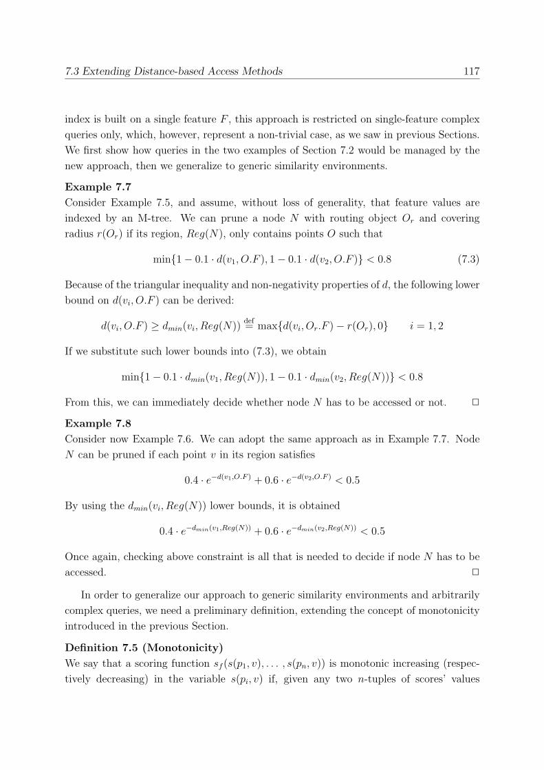
7.3 Extending Distance-based Access Methods 117
index is built on a single feature F , this approach is restricted on single-feature complex
queries only, which, however, represent a non-trivial case, as we saw in previous Sections.
We first show how queries in the two examples of Section 7.2 would be managed by the
new approach, then we generalize to generic similarity environments.
Example 7.7
Consider Example 7.5, and assume, without loss of generality, that feature values are
indexed by an M-tree. We can prune a node N with routing object Or and covering
radius r(Or) if its region, Reg(N), only contains points O such that
min{1− 0.1 · d(v1, O.F ), 1− 0.1 · d(v2, O.F )} < 0.8 (7.3)
Because of the triangular inequality and non-negativity properties of d, the following lower
bound on d(vi, O.F ) can be derived:
d(vi, O.F ) ≥ dmin(vi, Reg(N))def= max{d(vi, Or.F )− r(Or), 0} i = 1, 2
If we substitute such lower bounds into (7.3), we obtain
min{1− 0.1 · dmin(v1, Reg(N)), 1− 0.1 · dmin(v2, Reg(N))} < 0.8
From this, we can immediately decide whether node N has to be accessed or not. ✷
Example 7.8
Consider now Example 7.6. We can adopt the same approach as in Example 7.7. Node
N can be pruned if each point v in its region satisfies
0.4 · e−d(v1,O.F ) + 0.6 · e−d(v2,O.F ) < 0.5
By using the dmin(vi, Reg(N)) lower bounds, it is obtained
0.4 · e−dmin(v1,Reg(N)) + 0.6 · e−dmin(v2,Reg(N)) < 0.5
Once again, checking above constraint is all that is needed to decide if node N has to be
accessed. ✷
In order to generalize our approach to generic similarity environments and arbitrarily
complex queries, we need a preliminary definition, extending the concept of monotonicity
introduced in the previous Section.
Definition 7.5 (Monotonicity)
We say that a scoring function sf (s(p1, v), . . . , s(pn, v)) is monotonic increasing (respec-
tively decreasing) in the variable s(pi, v) if, given any two n-tuples of scores’ values
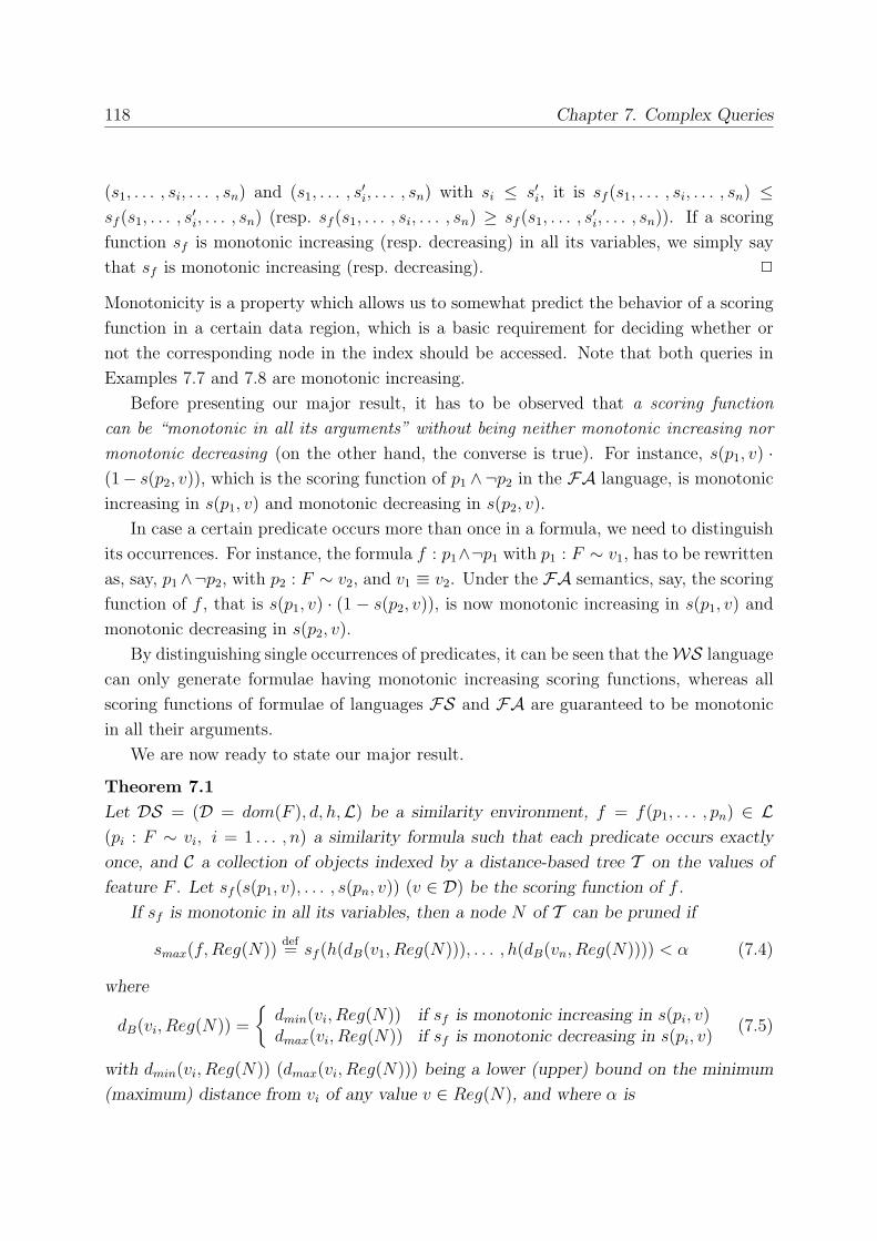
118 Chapter 7. Complex Queries
(s1, . . . , si, . . . , sn) and (s1, . . . , s′i, . . . , sn) with si ≤ s′i, it is sf (s1, . . . , si, . . . , sn) ≤
sf (s1, . . . , s′i, . . . , sn) (resp. sf (s1, . . . , si, . . . , sn) ≥ sf (s1, . . . , s
′i, . . . , sn)). If a scoring
function sf is monotonic increasing (resp. decreasing) in all its variables, we simply say
that sf is monotonic increasing (resp. decreasing). ✷
Monotonicity is a property which allows us to somewhat predict the behavior of a scoring
function in a certain data region, which is a basic requirement for deciding whether or
not the corresponding node in the index should be accessed. Note that both queries in
Examples 7.7 and 7.8 are monotonic increasing.
Before presenting our major result, it has to be observed that a scoring function
can be “monotonic in all its arguments” without being neither monotonic increasing nor
monotonic decreasing (on the other hand, the converse is true). For instance, s(p1, v) ·(1− s(p2, v)), which is the scoring function of p1 ∧¬p2 in the FA language, is monotonicincreasing in s(p1, v) and monotonic decreasing in s(p2, v).
In case a certain predicate occurs more than once in a formula, we need to distinguish
its occurrences. For instance, the formula f : p1∧¬p1 with p1 : F ∼ v1, has to be rewritten
as, say, p1∧¬p2, with p2 : F ∼ v2, and v1 ≡ v2. Under the FA semantics, say, the scoringfunction of f , that is s(p1, v) · (1 − s(p2, v)), is now monotonic increasing in s(p1, v) and
monotonic decreasing in s(p2, v).
By distinguishing single occurrences of predicates, it can be seen that theWS languagecan only generate formulae having monotonic increasing scoring functions, whereas all
scoring functions of formulae of languages FS and FA are guaranteed to be monotonic
in all their arguments.
We are now ready to state our major result.
Theorem 7.1
Let DS = (D = dom(F ), d, h,L) be a similarity environment, f = f(p1, . . . , pn) ∈ L(pi : F ∼ vi, i = 1 . . . , n) a similarity formula such that each predicate occurs exactly
once, and C a collection of objects indexed by a distance-based tree T on the values of
feature F . Let sf (s(p1, v), . . . , s(pn, v)) (v ∈ D) be the scoring function of f .
If sf is monotonic in all its variables, then a node N of T can be pruned if
smax(f,Reg(N))def= sf (h(dB(v1, Reg(N))), . . . , h(dB(vn, Reg(N)))) < α (7.4)
where
dB(vi, Reg(N)) =
{dmin(vi, Reg(N)) if sf is monotonic increasing in s(pi, v)dmax(vi, Reg(N)) if sf is monotonic decreasing in s(pi, v)
(7.5)
with dmin(vi, Reg(N)) (dmax(vi, Reg(N))) being a lower (upper) bound on the minimum
(maximum) distance from vi of any value v ∈ Reg(N), and where α is
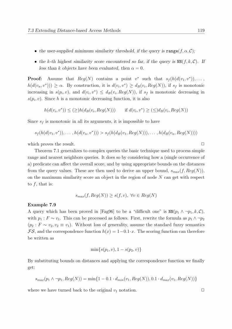
7.3 Extending Distance-based Access Methods 119
• the user-supplied minimum similarity threshold, if the query is range(f, α, C);
• the k-th highest similarity score encountered so far, if the query is NN(f, k, C). If
less than k objects have been evaluated, then α = 0.
Proof: Assume that Reg(N) contains a point v∗ such that sf (h(d(v1, v∗)), . . . ,
h(d(vn, v∗))) ≥ α. By construction, it is d(vi, v
∗) ≥ dB(vi, Reg(N)), if sf is monotonic
increasing in s(pi, v), and d(vi, v∗) ≤ dB(vi, Reg(N)), if sf is monotonic decreasing in
s(pi, v). Since h is a monotonic decreasing function, it is also
h(d(vi, v∗)) ≤ (≥)h(dB(vi, Reg(N))) if d(vi, v
∗) ≥ (≤)dB(vi, Reg(N))
Since sf is monotonic in all its arguments, it is impossible to have
sf (h(d(v1, v∗)), . . . , h(d(vn, v∗))) > sf (h(dB(v1, Reg(N))), . . . , h(dB(vn, Reg(N))))
which proves the result. ✷
Theorem 7.1 generalizes to complex queries the basic technique used to process simple
range and nearest neighbors queries. It does so by considering how a (single occurrence of
a) predicate can affect the overall score, and by using appropriate bounds on the distances
from the query values. These are then used to derive an upper bound, smax(f,Reg(N)),
on the maximum similarity score an object in the region of node N can get with respect
to f , that is:
smax(f,Reg(N)) ≥ s(f, v), ∀v ∈ Reg(N)
Example 7.9
A query which has been proved in [Fag96] to be a “difficult one” is NN(p1 ∧ ¬p1, k, C),with p1 : F ∼ v1. This can be processed as follows. First, rewrite the formula as p1 ∧¬p2
(p2 : F ∼ v2, v2 ≡ v1). Without loss of generality, assume the standard fuzzy semantics
FS, and the correspondence function h(x) = 1−0.1·x. The scoring function can thereforebe written as
min{s(p1, v), 1− s(p2, v)}
By substituting bounds on distances and applying the correspondence function we finally
get:
smax(p1 ∧ ¬p1, Reg(N)) = min{1− 0.1 · dmin(v1, Reg(N)), 0.1 · dmax(v1, Reg(N))}
where we have turned back to the original v1 notation. ✷
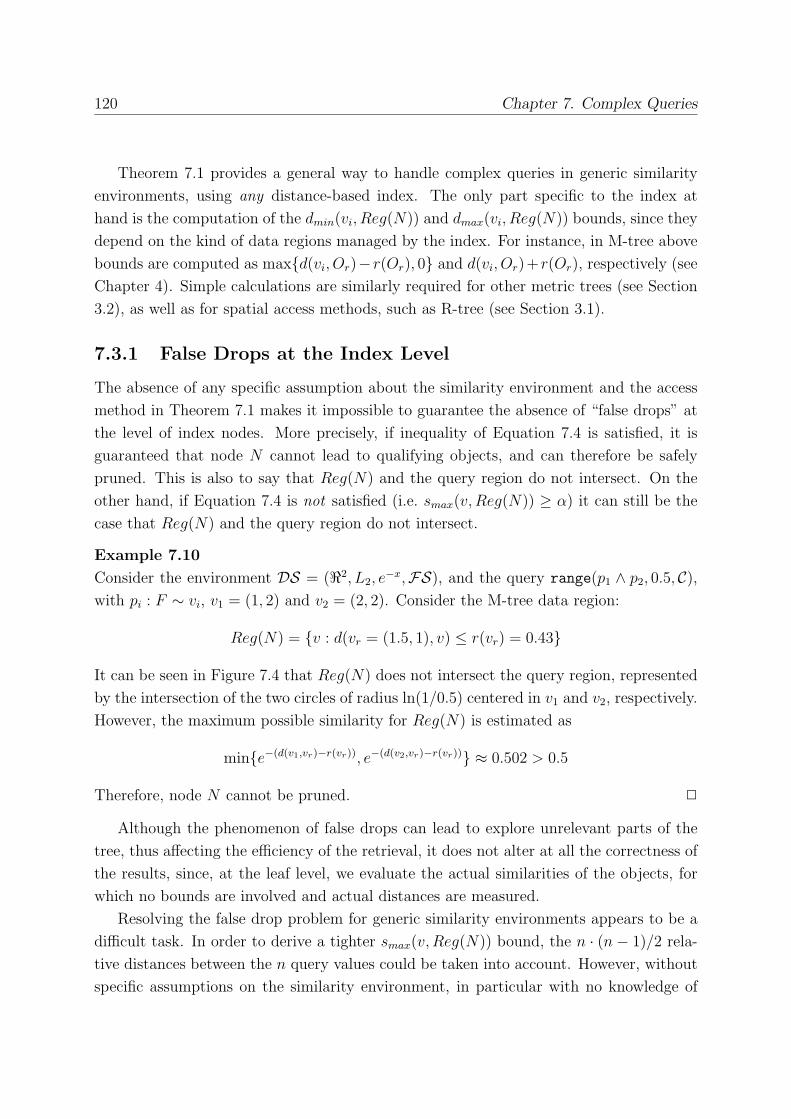
120 Chapter 7. Complex Queries
Theorem 7.1 provides a general way to handle complex queries in generic similarity
environments, using any distance-based index. The only part specific to the index at
hand is the computation of the dmin(vi, Reg(N)) and dmax(vi, Reg(N)) bounds, since they
depend on the kind of data regions managed by the index. For instance, in M-tree above
bounds are computed as max{d(vi, Or)−r(Or), 0} and d(vi, Or)+r(Or), respectively (see
Chapter 4). Simple calculations are similarly required for other metric trees (see Section
3.2), as well as for spatial access methods, such as R-tree (see Section 3.1).
7.3.1 False Drops at the Index Level
The absence of any specific assumption about the similarity environment and the access
method in Theorem 7.1 makes it impossible to guarantee the absence of “false drops” at
the level of index nodes. More precisely, if inequality of Equation 7.4 is satisfied, it is
guaranteed that node N cannot lead to qualifying objects, and can therefore be safely
pruned. This is also to say that Reg(N) and the query region do not intersect. On the
other hand, if Equation 7.4 is not satisfied (i.e. smax(v,Reg(N)) ≥ α) it can still be the
case that Reg(N) and the query region do not intersect.
Example 7.10
Consider the environment DS = (�2, L2, e−x,FS), and the query range(p1 ∧ p2, 0.5, C),
with pi : F ∼ vi, v1 = (1, 2) and v2 = (2, 2). Consider the M-tree data region:
Reg(N) = {v : d(vr = (1.5, 1), v) ≤ r(vr) = 0.43}
It can be seen in Figure 7.4 that Reg(N) does not intersect the query region, represented
by the intersection of the two circles of radius ln(1/0.5) centered in v1 and v2, respectively.
However, the maximum possible similarity for Reg(N) is estimated as
min{e−(d(v1,vr)−r(vr)), e−(d(v2,vr)−r(vr))} ≈ 0.502 > 0.5
Therefore, node N cannot be pruned. ✷
Although the phenomenon of false drops can lead to explore unrelevant parts of the
tree, thus affecting the efficiency of the retrieval, it does not alter at all the correctness of
the results, since, at the leaf level, we evaluate the actual similarities of the objects, for
which no bounds are involved and actual distances are measured.
Resolving the false drop problem for generic similarity environments appears to be a
difficult task. In order to derive a tighter smax(v,Reg(N)) bound, the n · (n− 1)/2 rela-tive distances between the n query values could be taken into account. However, without
specific assumptions on the similarity environment, in particular with no knowledge of
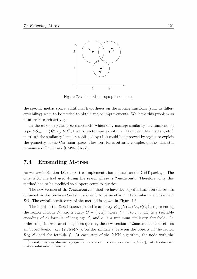
7.4 Extending M-tree 121
v2
vr
v12
1
21
Figure 7.4: The false drops phenomenon.
the specific metric space, additional hypotheses on the scoring functions (such as differ-
entiability) seem to be needed to obtain major improvements. We leave this problem as
a future research activity.
In the case of spatial access methods, which only manage similarity environments of
type DSsam = (�n, Lp, h,L), that is, vector spaces with Lp (Euclidean, Manhattan, etc.)
metrics,3 the similarity bound established by (7.4) could be improved by trying to exploit
the geometry of the Cartesian space. However, for arbitrarily complex queries this still
remains a difficult task [HM95, SK97].
7.4 Extending M-tree
As we saw in Section 4.6, our M-tree implementation is based on the GiST package. The
only GiST method used during the search phase is Consistent. Therefore, only this
method has to be modified to support complex queries.
The new version of the Consistent method we have developed is based on the results
obtained in the previous Section, and is fully parametric in the similarity environment
DS. The overall architecture of the method is shown in Figure 7.5.The input of the Consistent method is an entry Reg(N) ≡ (Or, r(Or)), representing
the region of node N , and a query Q ≡ (f, α), where f = f(p1, . . . , pn) is a (suitable
encoding of a) formula of language L, and α is a minimum similarity threshold. In
order to optimize nearest neighbors queries, the new version of Consistent also returns
an upper bound, smax(f,Reg(N)), on the similarity between the objects in the region
Reg(N) and the formula f . At each step of the k-NN algorithm, the node with the
3Indeed, they can also manage quadratic distance functions, as shown in [SK97], but this does notmake a substantial difference.
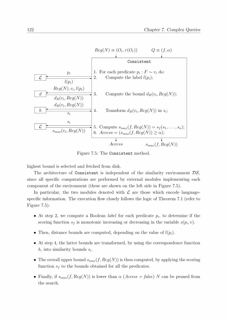
122 Chapter 7. Complex Queries
❄ ❄
Reg(N) ≡ (Or, r(Or)) Q ≡ (f, α)
Access smax(f,Reg(N))❄ ❄
Consistent
1. For each predicate pi : F ∼ vi do:2. Compute the label l(pi);
3. Compute the bound dB(vi, Reg(N));
4. Transform dB(vi, Reg(N)) in si;
5. Compute smax(f,Reg(N)) = sf (s1, . . . , sn);6. Access = (smax(f,Reg(N)) ≥ α);
✛ ✲Lpi
l(pi)
✛ ✲dReg(N), vi, l(pi)
dB(vi, Reg(N))
✛ ✲hdB(vi, Reg(N))
si
✛ ✲Lsi
smax(vi, Reg(N))
Figure 7.5: The Consistent method.
highest bound is selected and fetched from disk.
The architecture of Consistent is independent of the similarity environment DS,since all specific computations are performed by external modules implementing each
component of the environment (these are shown on the left side in Figure 7.5).
In particular, the two modules denoted with L are those which encode language-
specific information. The execution flow closely follows the logic of Theorem 7.1 (refer to
Figure 7.5):
• At step 2, we compute a Boolean label for each predicate pi, to determine if thescoring function sf is monotonic increasing or decreasing in the variable s(pi, v).
• Then, distance bounds are computed, depending on the value of l(pi).
• At step 4, the latter bounds are transformed, by using the correspondence functionh, into similarity bounds si.
• The overall upper bound smax(f,Reg(N)) is then computed, by applying the scoring
function sf to the bounds obtained for all the predicates.
• Finally, if smax(f,Reg(N)) is lower than α (Access = false) N can be pruned from
the search.
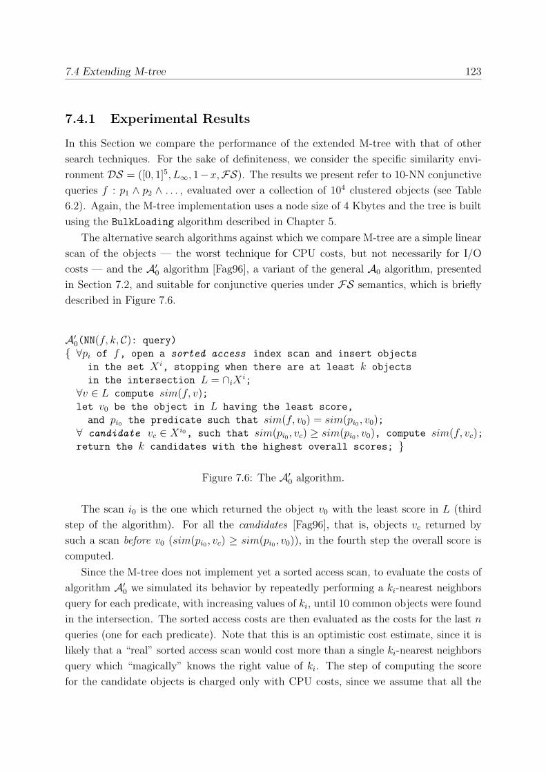
7.4 Extending M-tree 123
7.4.1 Experimental Results
In this Section we compare the performance of the extended M-tree with that of other
search techniques. For the sake of definiteness, we consider the specific similarity envi-
ronment DS = ([0, 1]5, L∞, 1−x,FS). The results we present refer to 10-NN conjunctivequeries f : p1 ∧ p2 ∧ . . . , evaluated over a collection of 104 clustered objects (see Table
6.2). Again, the M-tree implementation uses a node size of 4 Kbytes and the tree is built
using the BulkLoading algorithm described in Chapter 5.
The alternative search algorithms against which we compare M-tree are a simple linear
scan of the objects — the worst technique for CPU costs, but not necessarily for I/O
costs — and the A′0 algorithm [Fag96], a variant of the general A0 algorithm, presented
in Section 7.2, and suitable for conjunctive queries under FS semantics, which is brieflydescribed in Figure 7.6.
A′0(NN(f, k, C): query)
{ ∀pi of f, open a sorted access index scan and insert objects
in the set X i, stopping when there are at least k objects
in the intersection L = ∩iXi;
∀v ∈ L compute sim(f, v);let v0 be the object in L having the least score,
and pi0 the predicate such that sim(f, v0) = sim(pi0 , v0);∀ candidate vc ∈ X i0, such that sim(pi0 , vc) ≥ sim(pi0 , v0), compute sim(f, vc);return the k candidates with the highest overall scores; }
Figure 7.6: The A′0 algorithm.
The scan i0 is the one which returned the object v0 with the least score in L (third
step of the algorithm). For all the candidates [Fag96], that is, objects vc returned by
such a scan before v0 (sim(pi0 , vc) ≥ sim(pi0 , v0)), in the fourth step the overall score is
computed.
Since the M-tree does not implement yet a sorted access scan, to evaluate the costs of
algorithm A′0 we simulated its behavior by repeatedly performing a ki-nearest neighbors
query for each predicate, with increasing values of ki, until 10 common objects were found
in the intersection. The sorted access costs are then evaluated as the costs for the last n
queries (one for each predicate). Note that this is an optimistic cost estimate, since it is
likely that a “real” sorted access scan would cost more than a single ki-nearest neighbors
query which “magically” knows the right value of ki. The step of computing the score
for the candidate objects is charged only with CPU costs, since we assume that all the
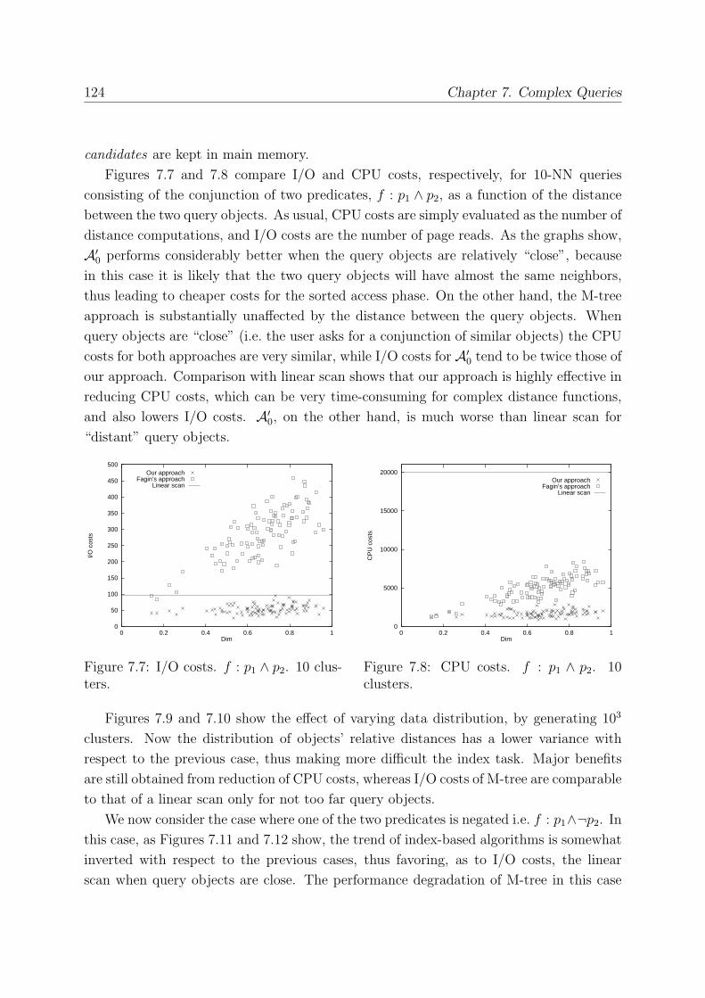
124 Chapter 7. Complex Queries
candidates are kept in main memory.
Figures 7.7 and 7.8 compare I/O and CPU costs, respectively, for 10-NN queries
consisting of the conjunction of two predicates, f : p1 ∧ p2, as a function of the distance
between the two query objects. As usual, CPU costs are simply evaluated as the number of
distance computations, and I/O costs are the number of page reads. As the graphs show,
A′0 performs considerably better when the query objects are relatively “close”, because
in this case it is likely that the two query objects will have almost the same neighbors,
thus leading to cheaper costs for the sorted access phase. On the other hand, the M-tree
approach is substantially unaffected by the distance between the query objects. When
query objects are “close” (i.e. the user asks for a conjunction of similar objects) the CPU
costs for both approaches are very similar, while I/O costs for A′0 tend to be twice those of
our approach. Comparison with linear scan shows that our approach is highly effective in
reducing CPU costs, which can be very time-consuming for complex distance functions,
and also lowers I/O costs. A′0, on the other hand, is much worse than linear scan for
“distant” query objects.
0
50
100
150
200
250
300
350
400
450
500
0 0.2 0.4 0.6 0.8 1
I/O c
osts
Dim
Our approachFagin’s approach
Linear scan
Figure 7.7: I/O costs. f : p1 ∧ p2. 10 clus-ters.
0
5000
10000
15000
20000
0 0.2 0.4 0.6 0.8 1
CP
U c
osts
Dim
Our approachFagin’s approach
Linear scan
Figure 7.8: CPU costs. f : p1 ∧ p2. 10clusters.
Figures 7.9 and 7.10 show the effect of varying data distribution, by generating 103
clusters. Now the distribution of objects’ relative distances has a lower variance with
respect to the previous case, thus making more difficult the index task. Major benefits
are still obtained from reduction of CPU costs, whereas I/O costs of M-tree are comparable
to that of a linear scan only for not too far query objects.
We now consider the case where one of the two predicates is negated i.e. f : p1∧¬p2. In
this case, as Figures 7.11 and 7.12 show, the trend of index-based algorithms is somewhat
inverted with respect to the previous cases, thus favoring, as to I/O costs, the linear
scan when query objects are close. The performance degradation of M-tree in this case
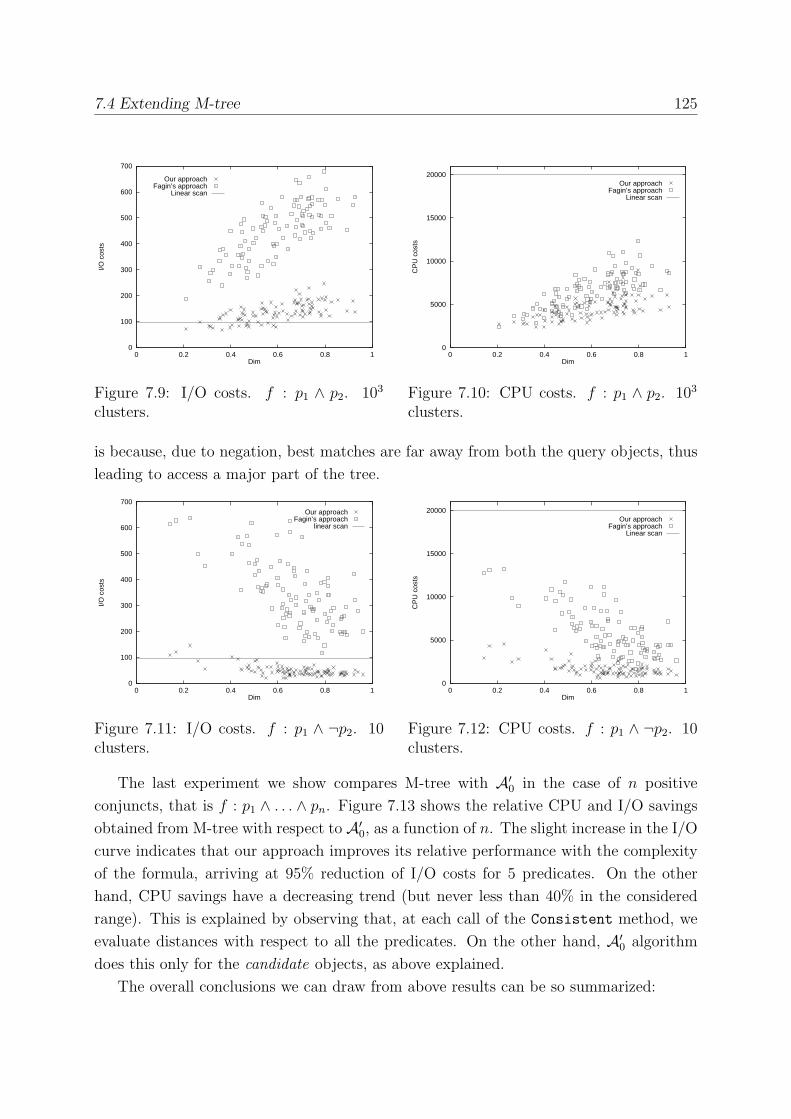
7.4 Extending M-tree 125
0
100
200
300
400
500
600
700
0 0.2 0.4 0.6 0.8 1
I/O c
osts
Dim
Our approachFagin’s approach
Linear scan
Figure 7.9: I/O costs. f : p1 ∧ p2. 103
clusters.
0
5000
10000
15000
20000
0 0.2 0.4 0.6 0.8 1
CP
U c
osts
Dim
Our approachFagin’s approach
Linear scan
Figure 7.10: CPU costs. f : p1 ∧ p2. 103
clusters.
is because, due to negation, best matches are far away from both the query objects, thus
leading to access a major part of the tree.
0
100
200
300
400
500
600
700
0 0.2 0.4 0.6 0.8 1
I/O c
osts
Dim
Our approachFagin’s approach
linear scan
Figure 7.11: I/O costs. f : p1 ∧ ¬p2. 10clusters.
0
5000
10000
15000
20000
0 0.2 0.4 0.6 0.8 1
CP
U c
osts
Dim
Our approachFagin’s approach
Linear scan
Figure 7.12: CPU costs. f : p1 ∧ ¬p2. 10clusters.
The last experiment we show compares M-tree with A′0 in the case of n positive
conjuncts, that is f : p1 ∧ . . . ∧ pn. Figure 7.13 shows the relative CPU and I/O savings
obtained from M-tree with respect to A′0, as a function of n. The slight increase in the I/O
curve indicates that our approach improves its relative performance with the complexity
of the formula, arriving at 95% reduction of I/O costs for 5 predicates. On the other
hand, CPU savings have a decreasing trend (but never less than 40% in the considered
range). This is explained by observing that, at each call of the Consistent method, we
evaluate distances with respect to all the predicates. On the other hand, A′0 algorithm
does this only for the candidate objects, as above explained.
The overall conclusions we can draw from above results can be so summarized:
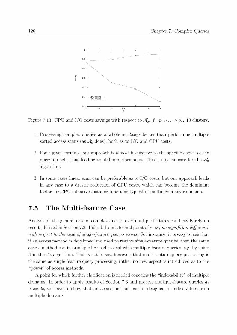
126 Chapter 7. Complex Queries
0.4
0.5
0.6
0.7
0.8
0.9
1
2 2.5 3 3.5 4 4.5 5
savi
ng
n
CPU savingI/O saving
Figure 7.13: CPU and I/O costs savings with respect to A′0. f : p1 ∧ . . .∧ pn. 10 clusters.
1. Processing complex queries as a whole is always better than performing multiple
sorted access scans (as A′0 does), both as to I/O and CPU costs.
2. For a given formula, our approach is almost insensitive to the specific choice of the
query objects, thus leading to stable performance. This is not the case for the A′0
algorithm.
3. In some cases linear scan can be preferable as to I/O costs, but our approach leads
in any case to a drastic reduction of CPU costs, which can become the dominant
factor for CPU-intensive distance functions typical of multimedia environments.
7.5 The Multi-feature Case
Analysis of the general case of complex queries over multiple features can heavily rely on
results derived in Section 7.3. Indeed, from a formal point of view, no significant difference
with respect to the case of single-feature queries exists. For instance, it is easy to see that
if an access method is developed and used to resolve single-feature queries, then the same
access method can in principle be used to deal with multiple-feature queries, e.g. by using
it in the A0 algorithm. This is not to say, however, that multi-feature query processing is
the same as single-feature query processing, rather no new aspect is introduced as to the
“power” of access methods.
A point for which further clarification is needed concerns the “indexability” of multiple
domains. In order to apply results of Section 7.3 and process multiple-feature queries as
a whole, we have to show that an access method can be designed to index values from
multiple domains.
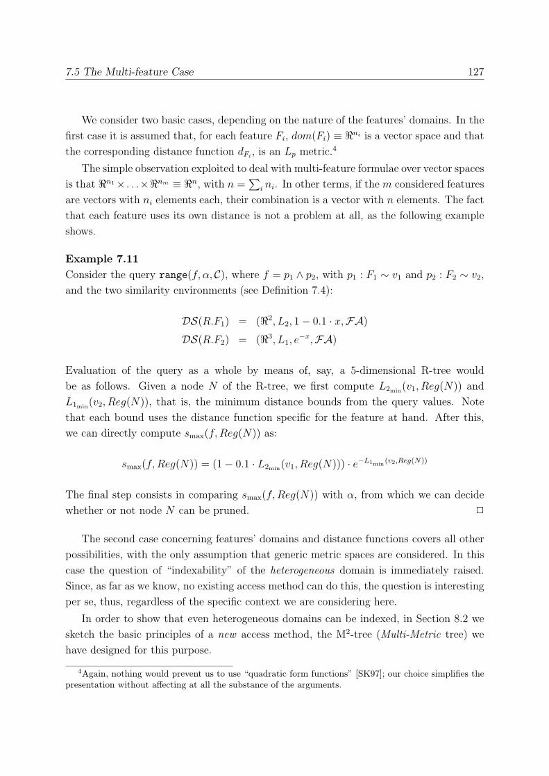
7.5 The Multi-feature Case 127
We consider two basic cases, depending on the nature of the features’ domains. In the
first case it is assumed that, for each feature Fi, dom(Fi) ≡ �ni is a vector space and that
the corresponding distance function dFi, is an Lp metric.
4
The simple observation exploited to deal with multi-feature formulae over vector spaces
is that �n1× . . .×�nm ≡ �n, with n =∑
i ni. In other terms, if the m considered features
are vectors with ni elements each, their combination is a vector with n elements. The fact
that each feature uses its own distance is not a problem at all, as the following example
shows.
Example 7.11
Consider the query range(f, α, C), where f = p1 ∧ p2, with p1 : F1 ∼ v1 and p2 : F2 ∼ v2,
and the two similarity environments (see Definition 7.4):
DS(R.F1) = (�2, L2, 1− 0.1 · x,FA)DS(R.F2) = (�3, L1, e
−x,FA)
Evaluation of the query as a whole by means of, say, a 5-dimensional R-tree would
be as follows. Given a node N of the R-tree, we first compute L2min(v1, Reg(N)) and
L1min(v2, Reg(N)), that is, the minimum distance bounds from the query values. Note
that each bound uses the distance function specific for the feature at hand. After this,
we can directly compute smax(f,Reg(N)) as:
smax(f,Reg(N)) = (1− 0.1 · L2min(v1, Reg(N))) · e−L1min
(v2,Reg(N))
The final step consists in comparing smax(f,Reg(N)) with α, from which we can decide
whether or not node N can be pruned. ✷
The second case concerning features’ domains and distance functions covers all other
possibilities, with the only assumption that generic metric spaces are considered. In this
case the question of “indexability” of the heterogeneous domain is immediately raised.
Since, as far as we know, no existing access method can do this, the question is interesting
per se, thus, regardless of the specific context we are considering here.
In order to show that even heterogeneous domains can be indexed, in Section 8.2 we
sketch the basic principles of a new access method, the M2-tree (Multi-Metric tree) we
have designed for this purpose.
4Again, nothing would prevent us to use “quadratic form functions” [SK97]; our choice simplifies thepresentation without affecting at all the substance of the arguments.
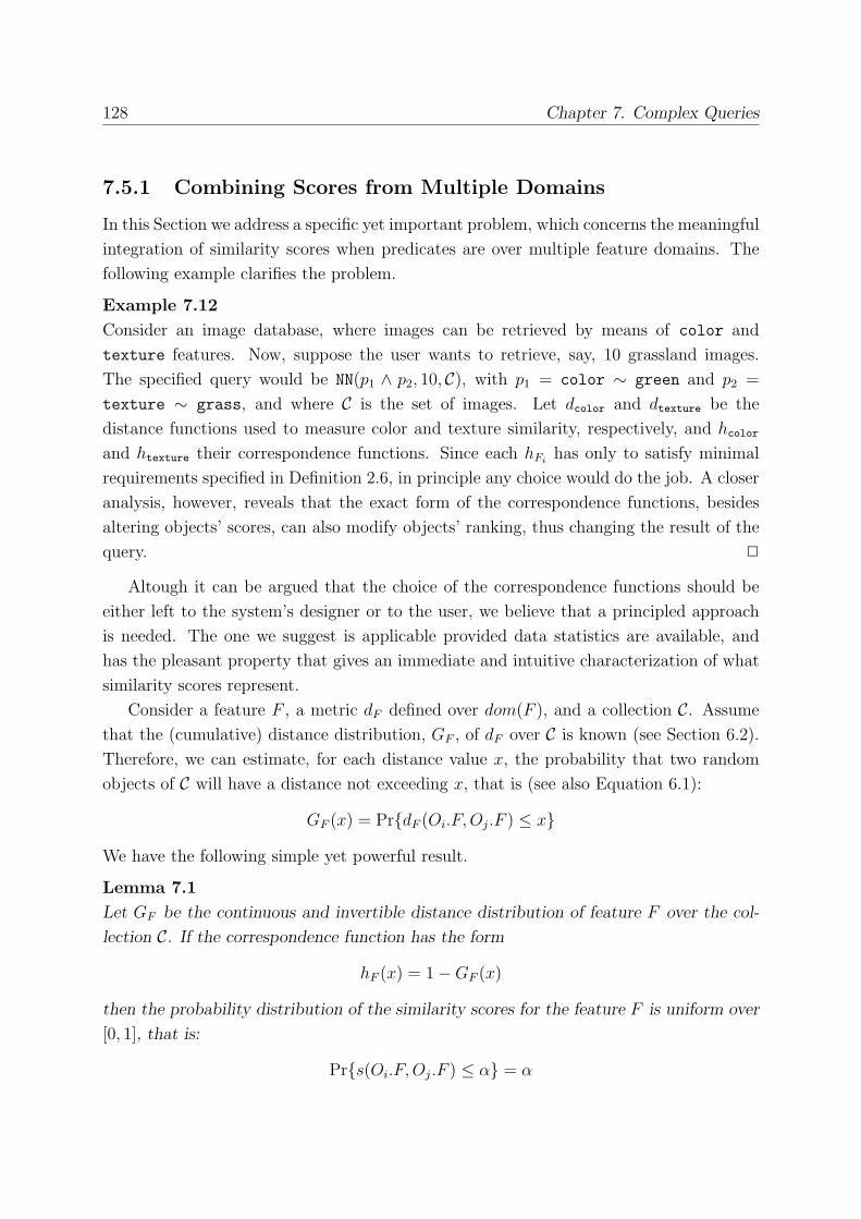
128 Chapter 7. Complex Queries
7.5.1 Combining Scores from Multiple Domains
In this Section we address a specific yet important problem, which concerns the meaningful
integration of similarity scores when predicates are over multiple feature domains. The
following example clarifies the problem.
Example 7.12
Consider an image database, where images can be retrieved by means of color and
texture features. Now, suppose the user wants to retrieve, say, 10 grassland images.
The specified query would be NN(p1 ∧ p2, 10, C), with p1 = color ∼ green and p2 =
texture ∼ grass, and where C is the set of images. Let dcolor and dtexture be the
distance functions used to measure color and texture similarity, respectively, and hcolor
and htexture their correspondence functions. Since each hFihas only to satisfy minimal
requirements specified in Definition 2.6, in principle any choice would do the job. A closer
analysis, however, reveals that the exact form of the correspondence functions, besides
altering objects’ scores, can also modify objects’ ranking, thus changing the result of the
query. ✷
Altough it can be argued that the choice of the correspondence functions should be
either left to the system’s designer or to the user, we believe that a principled approach
is needed. The one we suggest is applicable provided data statistics are available, and
has the pleasant property that gives an immediate and intuitive characterization of what
similarity scores represent.
Consider a feature F , a metric dF defined over dom(F ), and a collection C. Assumethat the (cumulative) distance distribution, GF , of dF over C is known (see Section 6.2).Therefore, we can estimate, for each distance value x, the probability that two random
objects of C will have a distance not exceeding x, that is (see also Equation 6.1):
GF (x) = Pr{dF (Oi.F,Oj.F ) ≤ x}
We have the following simple yet powerful result.
Lemma 7.1
Let GF be the continuous and invertible distance distribution of feature F over the col-
lection C. If the correspondence function has the form
hF (x) = 1−GF (x)
then the probability distribution of the similarity scores for the feature F is uniform over
[0, 1], that is:
Pr{s(Oi.F,Oj.F ) ≤ α} = α
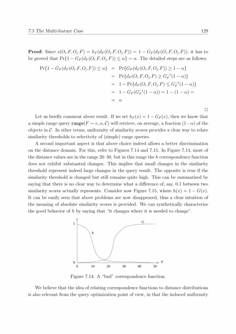
7.5 The Multi-feature Case 129
Proof: Since s(Oi.F,Oj.F ) = hF (dF (Oi.F,Oj.F )) = 1 − GF (dF (Oi.F,Oj.F )), it has to
be proved that Pr{1−GF (dF (Oi.F,Oj.F )) ≤ α} = α. The detailed steps are as follows:
Pr{1−GF (dF (Oi.F,Oj.F )) ≤ α} = Pr{GF (dF (Oi.F,Oj.F )) ≥ 1− α}= Pr{dF (Oi.F,Oj.F ) ≥ G−1
F (1− α)}= 1− Pr{dF (Oi.F,Oj.F ) ≤ G−1
F (1− α)}= 1−GF (G
−1F (1− α)) = 1− (1− α) =
= α
✷
Let us briefly comment above result. If we set hF (x) = 1−GF (x), then we know that
a simple range query range(F ∼ v, α, C) will retrieve, on average, a fraction (1 - α) of theobjects in C. In other terms, uniformity of similarity scores provides a clear way to relatesimilarity thresholds to selectivity of (simple) range queries.
A second important aspect is that above choice indeed allows a better discrimination
on the distance domain. For this, refer to Figures 7.14 and 7.15. In Figure 7.14, most of
the distance values are in the range 20–30, but in this range the h correspondence function
does not exhibit substantial changes. This implies that small changes in the similarity
threshold represent indeed large changes in the query result. The opposite is true if the
similarity threshold is changed but still remains quite high. This can be summarized by
saying that there is no clear way to determine what a difference of, say, 0.1 between two
similarity scores actually represents. Consider now Figure 7.15, where h(x) = 1 − G(x).
It can be easily seen that above problems are now disappeared, thus a clear intuition of
the meaning of absolute similarity scores is provided. We can synthetically characterize
the good behavior of h by saying that “it changes where it is needed to change”.
d0 10 20 30 40 50
0
1 G
h
Figure 7.14: A “bad” correspondence function.
We believe that the idea of relating correspondence functions to distance distributions
is also relevant from the query optimization point of view, in that the induced uniformity
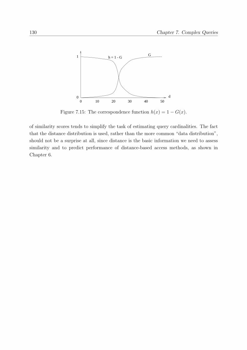
130 Chapter 7. Complex Queries
d0 10 20 30 40 50
0
1 Gh = 1 - G
Figure 7.15: The correspondence function h(x) = 1−G(x).
of similarity scores tends to simplify the task of estimating query cardinalities. The fact
that the distance distribution is used, rather than the more common “data distribution”,
should not be a surprise at all, since distance is the basic information we need to assess
similarity and to predict performance of distance-based access methods, as shown in
Chapter 6.
Chapter 8
Limitations and Extensions of M-tree
In Chapter 4 we showed the effectiveness of the M-tree access structure for the efficient
indexing of generic metric spaces. We also pointed out that, unlike the R-tree family of
index methods, the M-tree is not restricted to vector spaces. The conclusion that M-tree
is a generalization of R-tree is, however, not true, as explained by the following points:
• First of all, R-tree-like indices can take advantage of the use of objects’ coordinatesto organize the space; of course, such information is not available in a generic metric
space.
• SAMs are easily extendible to deal with user-adaptable similarity queries, i.e. withqueries referring to user-defined distance functions [SK97]. From the definition of
the M-tree given in Chapter 4, it seems that the only supported distance function
for queries is the same metric used to build the tree.
In this Chapter, we will “extend” the M-tree to deal with queries using a different
metric with respect to that used to build the tree. Then, we will present the M2-tree, a
novel index structure generalizing both the M-tree and the R-tree access methods. Such
index structure can be effectively used to deal with complex queries referring to multiple
domains (see Section 7.5).
8.1 Using Different Metrics with M-tree
In Section 4.2 we proved, by way of Lemma 4.1, that if the distance between the query
object Q and the routing object Or of a node is greater than the sum of the query
radius rQ and of the covering radius r(Or) of the node, that is if d(Q,Or) > rQ + r(Or),
then the sub-tree rooted at that node, i.e. T (Or), can be safely pruned from the search,
thus guaranteeing the absence of false dismissals, i.e. objects satisfying the query but
131
132 Chapter 8. Limitations and Extensions of M-tree
not included in the result set. This, as stated in Section 1.1, is one of the fundamental
properties for the similarity search process. If we are to generalize the M-tree access
method in order to make it able to deal with distance functions different from that used
to build the tree, we should, therefore, guarantee that, in any case, no false dismissal is
present. To this end, we start by precisely defining our reference scenario.
In the general case, three different metrics can be used with an M-tree:
1. the indexing distance function, dI , that is used to build the tree,
2. the query distance function, dq, used to issue queries to the system, and
3. the comparison distance function, dc, used to compare the query object and the
objects stored in the tree during the search phase.
For pruning sub-parts of the tree during the search phase, we have to find a pruning
criterion similar to that of Lemma 4.1. This is provided by the following
Lemma 8.1
If dc is a lower bounding distance function for both dI and dq and dc(Or, Q) > rQ+ r(Or),
then, for each object Oj in T (Or), it is dq(Oj, Q) > rQ. Thus, T (Or) can be safely pruned
from the search.
Proof: We have to prove that, if dc(Or, Q) > rQ+ r(Or) and dI(Or, Oj) ≤ r(Or), then it
is dq(Q,Oj) > rQ. In fact, it is
dq(Q,Oj) ≥ dc(Q,Oj) (def. of l.b. distance function) (8.1)
≥ dc(Q,Or)− dc(Or, Oj) (triangle inequality)
≥ dc(Q,Or)− dI(Or, Oj) (def. of l.b. distance function)
≥ dc(Q,Or)− r(Or) (def. of covering radius)
> rQ + r(Or)− r(Or) (by hypothesis)
= rQ
✷
From Lemma 8.1, we see that, in order to search without false dismissals the M-tree
using a distance function different from that used to build the tree, it is sufficient (and
also necessary as it can be easily proven) to provide a comparison function that is a lower
bound for both the indexing and the query metrics (see Definition 3.1).
For each internal node, therefore, we compute the comparison distance between the
query object Q and the routing object of the node Or and apply Lemma 8.1. In order
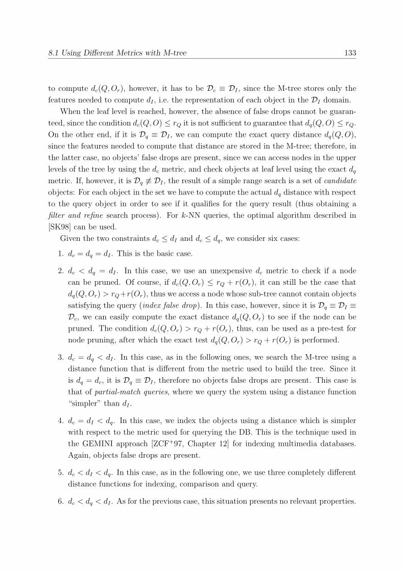
8.1 Using Different Metrics with M-tree 133
to compute dc(Q,Or), however, it has to be Dc ≡ DI , since the M-tree stores only the
features needed to compute dI , i.e. the representation of each object in the DI domain.
When the leaf level is reached, however, the absence of false drops cannot be guaran-
teed, since the condition dc(Q,O) ≤ rQ it is not sufficient to guarantee that dq(Q,O) ≤ rQ.
On the other end, if it is Dq ≡ DI , we can compute the exact query distance dq(Q,O),
since the features needed to compute that distance are stored in the M-tree; therefore, in
the latter case, no objects’ false drops are present, since we can access nodes in the upper
levels of the tree by using the dc metric, and check objects at leaf level using the exact dq
metric. If, however, it is Dq ≡ DI , the result of a simple range search is a set of candidate
objects: For each object in the set we have to compute the actual dq distance with respect
to the query object in order to see if it qualifies for the query result (thus obtaining a
filter and refine search process). For k-NN queries, the optimal algorithm described in
[SK98] can be used.
Given the two constraints dc ≤ dI and dc ≤ dq, we consider six cases:
1. dc = dq = dI . This is the basic case.
2. dc < dq = dI . In this case, we use an unexpensive dc metric to check if a node
can be pruned. Of course, if dc(Q,Or) ≤ rQ + r(Or), it can still be the case that
dq(Q,Or) > rQ+r(Or), thus we access a node whose sub-tree cannot contain objects
satisfying the query (index false drop). In this case, however, since it is Dq ≡ DI ≡Dc, we can easily compute the exact distance dq(Q,Or) to see if the node can be
pruned. The condition dc(Q,Or) > rQ + r(Or), thus, can be used as a pre-test for
node pruning, after which the exact test dq(Q,Or) > rQ + r(Or) is performed.
3. dc = dq < dI . In this case, as in the following ones, we search the M-tree using a
distance function that is different from the metric used to build the tree. Since it
is dq = dc, it is Dq ≡ DI , therefore no objects false drops are present. This case is
that of partial-match queries, where we query the system using a distance function
“simpler” than dI .
4. dc = dI < dq. In this case, we index the objects using a distance which is simpler
with respect to the metric used for querying the DB. This is the technique used in
the GEMINI approach [ZCF+97, Chapter 12] for indexing multimedia databases.
Again, objects false drops are present.
5. dc < dI < dq. In this case, as in the following one, we use three completely different
distance functions for indexing, comparison and query.
6. dc < dq < dI . As for the previous case, this situation presents no relevant properties.
134 Chapter 8. Limitations and Extensions of M-tree
8.1.1 False Drops at the Index Level
Another problem arising when using different metrics is that of index false drops. We
have an index false drop during the search phase when we access a branch of the tree that
cannot lead to any qualifying object. This problem is not present in the basic case when
dc = dq = dI , since the condition of Lemma 4.1 is also a necessary condition for pruning
a sub-tree. In order to prove that, we need a preliminary definition.
Definition 8.1 (Overlap of regions of a metric space)
Let Reg(O1) = (O1, r(O1)) and Reg(O2) = (O2, r(O2)) be two regions (balls) of a metric
spaceM = (D, d) defined as
Reg(Oi) = {x ∈ D : d(Oi, x) ≤ r(Oi)} (8.2)
We say that Reg(O1) and Reg(O2) overlap, if it cannot be excluded that
∃x ∈ D : x ∈ Reg(O1) ∧ x ∈ Reg(O2)
✷
Note that, in the general case, we cannot say that two regions of a metric space are
not overlapping if ∃x ∈ D : x ∈ Reg(O1)∧ x ∈ Reg(O2). As an example, see Figure 8.1,
representing the overlap of two regions in the (N2, L2) metric space: In this case the two
regions overlap, but there is no object of the space belonging to both regions, i.e. the two
regions are not intersecting. However, since the absence of objects in the intersection of
the two regions cannot be guaranteed for a generic metric space, for indexing purposes
we say that the two regions of Figure 8.1 actually overlap.
In order to exclude false drops, since the condition for node pruning is based on the
overlap between the node and the query regions, we have to prove that every accessed
node overlaps with the query region. In the exact case, i.e. when dc = dq = dI , no index
false drops are present, since the condition of Lemma 4.1 is not only sufficient but also
necessary to guarantee that two regions of the metric space do not overlap, as is specified
by the following
Theorem 8.1
Consider a query region Reg(Q) = (Q, rQ) and a node region Reg(Or) = (Or, r(Or)) of a
metric space M = (D, d). Then it is
d(Q,Or) > rQ + r(Or)⇔ Reg(Q) ¬overlaps Reg(Or) (8.3)
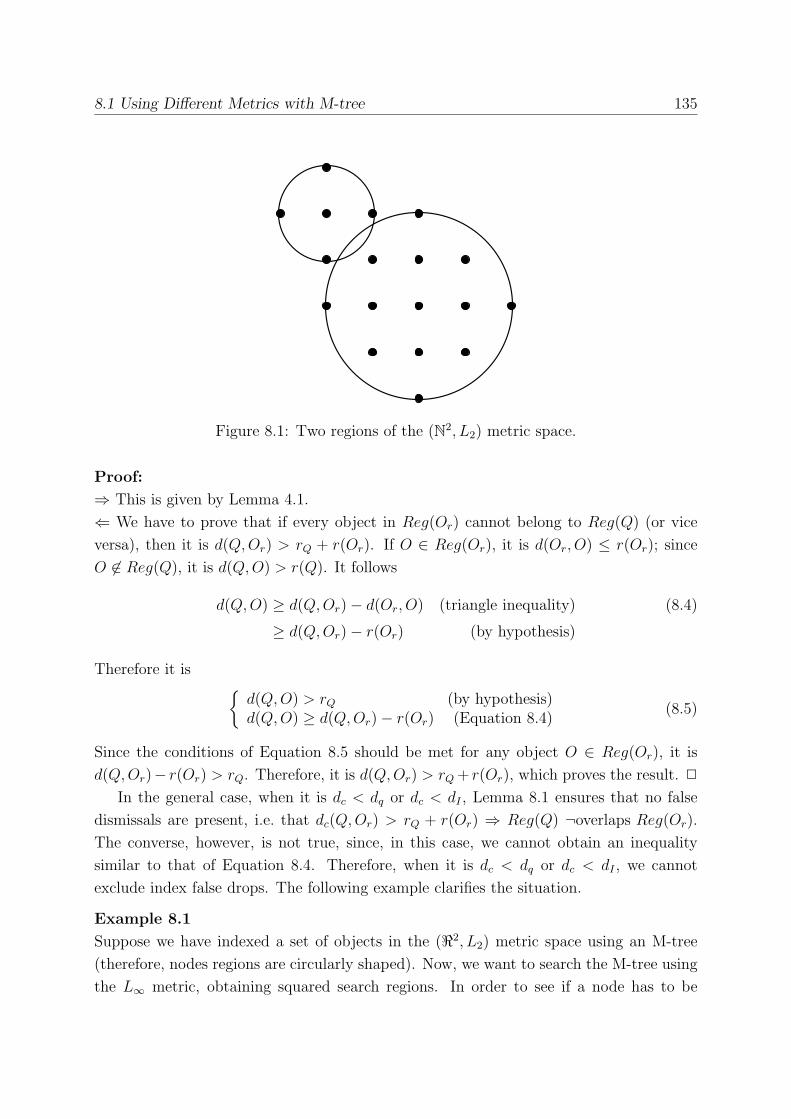
8.1 Using Different Metrics with M-tree 135
Figure 8.1: Two regions of the (N2, L2) metric space.
Proof:
⇒ This is given by Lemma 4.1.
⇐ We have to prove that if every object in Reg(Or) cannot belong to Reg(Q) (or vice
versa), then it is d(Q,Or) > rQ + r(Or). If O ∈ Reg(Or), it is d(Or, O) ≤ r(Or); since
O ∈ Reg(Q), it is d(Q,O) > r(Q). It follows
d(Q,O) ≥ d(Q,Or)− d(Or, O) (triangle inequality) (8.4)
≥ d(Q,Or)− r(Or) (by hypothesis)
Therefore it is {d(Q,O) > rQ (by hypothesis)d(Q,O) ≥ d(Q,Or)− r(Or) (Equation 8.4)
(8.5)
Since the conditions of Equation 8.5 should be met for any object O ∈ Reg(Or), it is
d(Q,Or)− r(Or) > rQ. Therefore, it is d(Q,Or) > rQ+ r(Or), which proves the result. ✷
In the general case, when it is dc < dq or dc < dI , Lemma 8.1 ensures that no false
dismissals are present, i.e. that dc(Q,Or) > rQ + r(Or) ⇒ Reg(Q) ¬overlaps Reg(Or).
The converse, however, is not true, since, in this case, we cannot obtain an inequality
similar to that of Equation 8.4. Therefore, when it is dc < dq or dc < dI , we cannot
exclude index false drops. The following example clarifies the situation.
Example 8.1
Suppose we have indexed a set of objects in the (�2, L2) metric space using an M-tree
(therefore, nodes regions are circularly shaped). Now, we want to search the M-tree using
the L∞ metric, obtaining squared search regions. In order to see if a node has to be
136 Chapter 8. Limitations and Extensions of M-tree
accessed, we compute the L∞ distance between the query object and the routing object
of the node. If this distance is higher than rQ + r(Or), we can safely prune the node.
Therefore, both the query radius and the node covering radius are considered with respect
to the dc metric function, L∞ in this case. In the case of Figure 8.2, the query region and
the node region are not overlapping. However, when the node region is “inflated” using
the L∞ metric, it overlaps with the query region; therefore, the node cannot be pruned
from the search and we access a node that cannot lead to qualifying objects.
rO
r
r(O )
Q
r
Q
Figure 8.2: An index false drop arising when we use, to query the M-tree, a distancefunction that is different from that used to build the tree.
✷
8.2 The M2-tree
The M-tree is able to index objects drawn from a metric spaceM. In order to extend this
access method to deal with multi-feature queries (see Section 7.5), we need to precisely
define our working scenario.
Definition 8.2 (Multi-dimensional metric space)
If {Mi = (Di, di), i = 1, . . . , n} is a set of metric spaces, we define the multi-dimensionalmetric space asMn = (D1 × . . .×Dn, (d1, . . . , dn)). ✷
In practice, a set of metric spaces defines a multi-dimensional metric space, whose
domain is given by the cartesian product of the domains of the original metric spaces. On
this domain, we can use the original distances to compare objects.
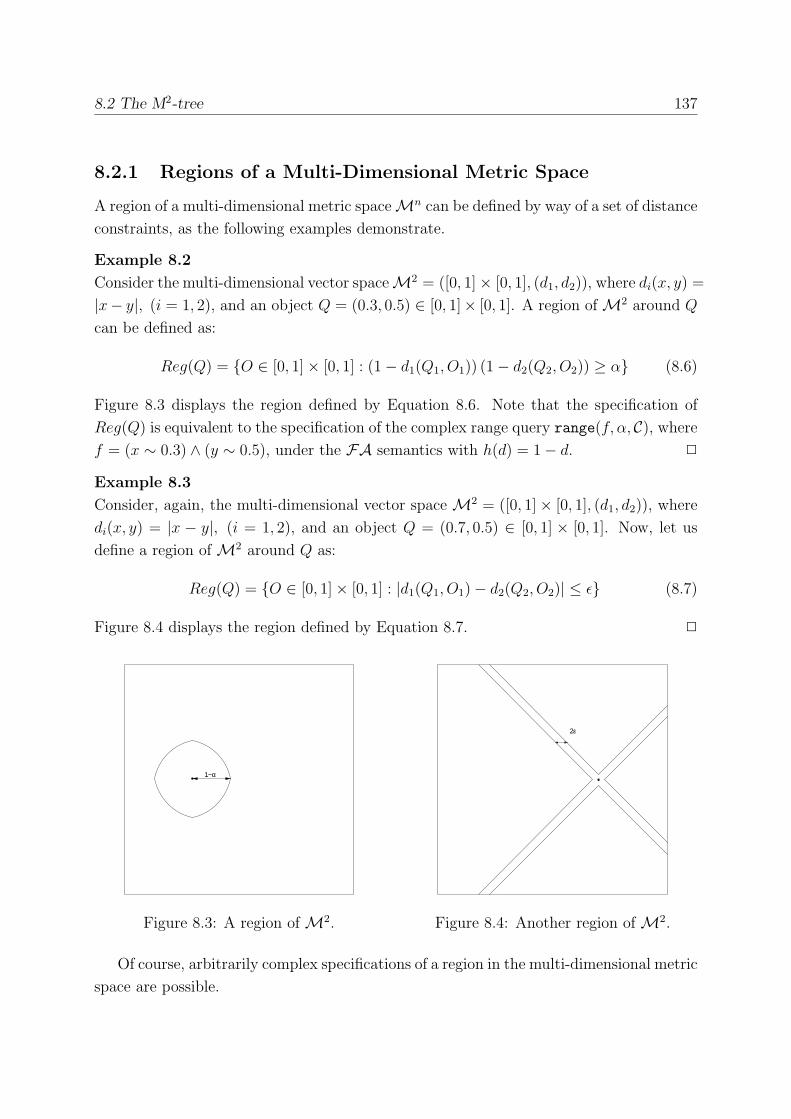
8.2 The M2-tree 137
8.2.1 Regions of a Multi-Dimensional Metric Space
A region of a multi-dimensional metric spaceMn can be defined by way of a set of distance
constraints, as the following examples demonstrate.
Example 8.2
Consider the multi-dimensional vector spaceM2 = ([0, 1]× [0, 1], (d1, d2)), where di(x, y) =
|x− y|, (i = 1, 2), and an object Q = (0.3, 0.5) ∈ [0, 1]× [0, 1]. A region ofM2 around Q
can be defined as:
Reg(Q) = {O ∈ [0, 1]× [0, 1] : (1− d1(Q1, O1)) (1− d2(Q2, O2)) ≥ α} (8.6)
Figure 8.3 displays the region defined by Equation 8.6. Note that the specification of
Reg(Q) is equivalent to the specification of the complex range query range(f, α, C), wheref = (x ∼ 0.3) ∧ (y ∼ 0.5), under the FA semantics with h(d) = 1− d. ✷
Example 8.3
Consider, again, the multi-dimensional vector spaceM2 = ([0, 1]× [0, 1], (d1, d2)), where
di(x, y) = |x − y|, (i = 1, 2), and an object Q = (0.7, 0.5) ∈ [0, 1] × [0, 1]. Now, let usdefine a region ofM2 around Q as:
Reg(Q) = {O ∈ [0, 1]× [0, 1] : |d1(Q1, O1)− d2(Q2, O2)| ≤ ε} (8.7)
Figure 8.4 displays the region defined by Equation 8.7. ✷
1−α
Figure 8.3: A region ofM2.
2ε
Figure 8.4: Another region ofM2.
Of course, arbitrarily complex specifications of a region in the multi-dimensional metric
space are possible.
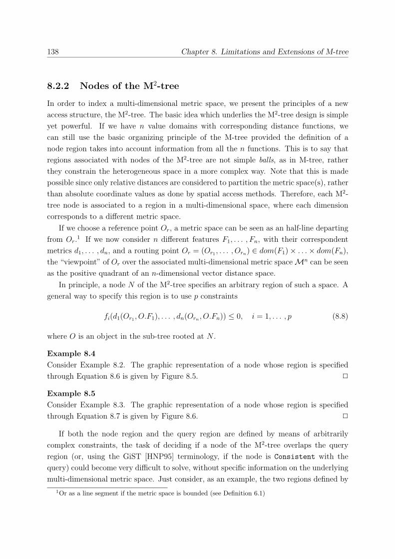
138 Chapter 8. Limitations and Extensions of M-tree
8.2.2 Nodes of the M2-tree
In order to index a multi-dimensional metric space, we present the principles of a new
access structure, the M2-tree. The basic idea which underlies the M2-tree design is simple
yet powerful. If we have n value domains with corresponding distance functions, we
can still use the basic organizing principle of the M-tree provided the definition of a
node region takes into account information from all the n functions. This is to say that
regions associated with nodes of the M2-tree are not simple balls, as in M-tree, rather
they constrain the heterogeneous space in a more complex way. Note that this is made
possible since only relative distances are considered to partition the metric space(s), rather
than absolute coordinate values as done by spatial access methods. Therefore, each M2-
tree node is associated to a region in a multi-dimensional space, where each dimension
corresponds to a different metric space.
If we choose a reference point Or, a metric space can be seen as an half-line departing
from Or.1 If we now consider n different features F1, . . . , Fn, with their correspondent
metrics d1, . . . , dn, and a routing point Or = (Or1 , . . . , Orn) ∈ dom(F1)× . . .× dom(Fn),
the “viewpoint” of Or over the associated multi-dimensional metric spaceMn can be seen
as the positive quadrant of an n-dimensional vector distance space.
In principle, a node N of the M2-tree specifies an arbitrary region of such a space. A
general way to specify this region is to use p constraints
fi(d1(Or1 , O.F1), . . . , dn(Orn , O.Fn)) ≤ 0, i = 1, . . . , p (8.8)
where O is an object in the sub-tree rooted at N .
Example 8.4
Consider Example 8.2. The graphic representation of a node whose region is specified
through Equation 8.6 is given by Figure 8.5. ✷
Example 8.5
Consider Example 8.3. The graphic representation of a node whose region is specified
through Equation 8.7 is given by Figure 8.6. ✷
If both the node region and the query region are defined by means of arbitrarily
complex constraints, the task of deciding if a node of the M2-tree overlaps the query
region (or, using the GiST [HNP95] terminology, if the node is Consistent with the
query) could become very difficult to solve, without specific information on the underlying
multi-dimensional metric space. Just consider, as an example, the two regions defined by
1Or as a line segment if the metric space is bounded (see Definition 6.1)
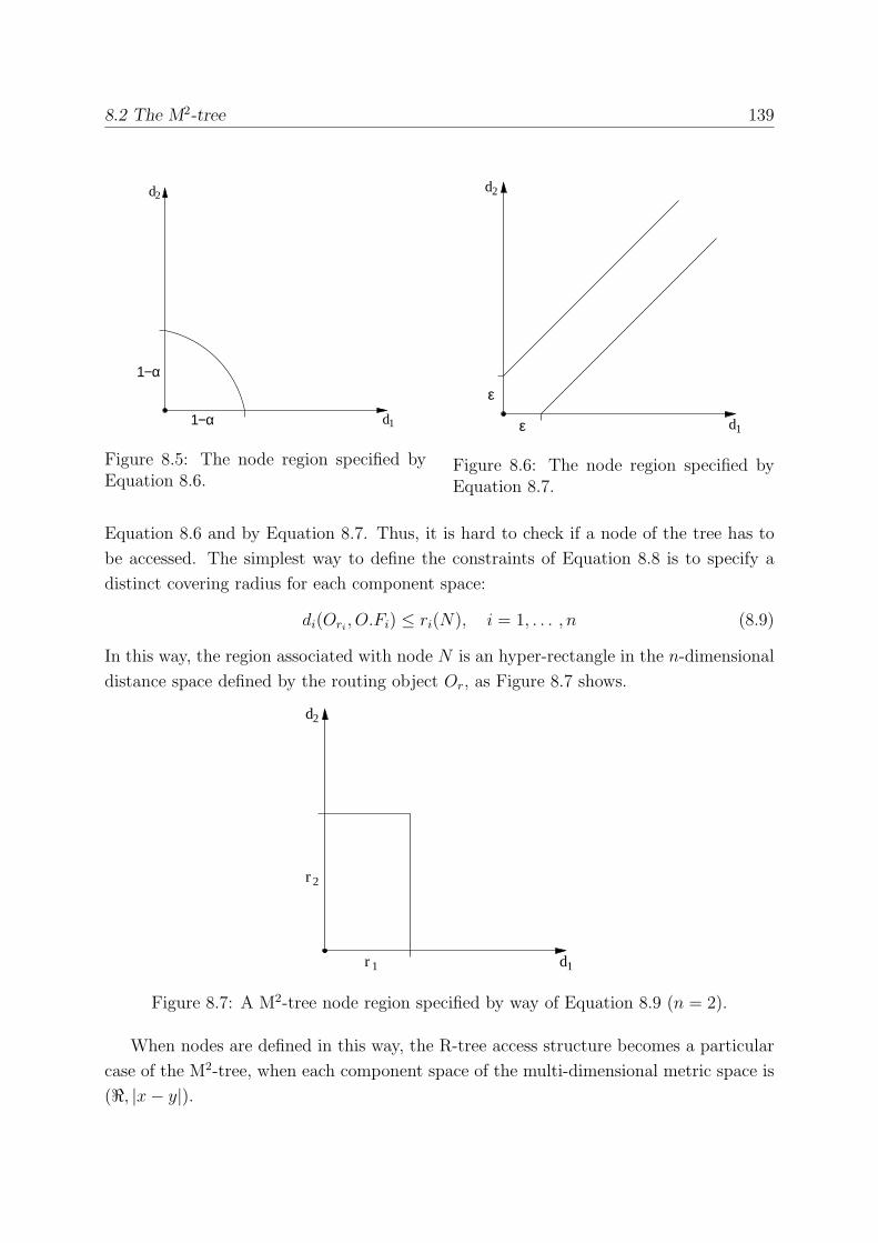
8.2 The M2-tree 139
d1
d2
1−α
1−α
Figure 8.5: The node region specified byEquation 8.6.
d1
d2
ε
ε
Figure 8.6: The node region specified byEquation 8.7.
Equation 8.6 and by Equation 8.7. Thus, it is hard to check if a node of the tree has to
be accessed. The simplest way to define the constraints of Equation 8.8 is to specify a
distinct covering radius for each component space:
di(Ori, O.Fi) ≤ ri(N), i = 1, . . . , n (8.9)
In this way, the region associated with node N is an hyper-rectangle in the n-dimensional
distance space defined by the routing object Or, as Figure 8.7 shows.
d1
d2
r 2
r 1
Figure 8.7: A M2-tree node region specified by way of Equation 8.9 (n = 2).
When nodes are defined in this way, the R-tree access structure becomes a particular
case of the M2-tree, when each component space of the multi-dimensional metric space is
(�, |x− y|).
140 Chapter 8. Limitations and Extensions of M-tree
Having defined how regions associated to M2-tree nodes are specified, we are now
ready to show how to search the tree. Given the query specification, thus, we have to
specify a criterion to prune sub-parts of the tree that cannot lead to qualifying objects. In
order to simplify the presentation, in the following we will only consider queries specified
through a similarity formula f , as defined in Section 7.1. In this scenario, Theorem 7.1
can easily be extended in order to be applied to M2-tree nodes.
Theorem 8.2
Let DSn = (D = dom(F1) × . . . × dom(Fn), (d1, . . . , dn), (h1, . . . , hn),L) be a multi-
similarity environment where similarity between objects can be assessed by way of n
different distance functions di on the domain D, each with the respective correspondence
function hi; let f = f(p1, . . . , pm) ∈ L (pj : Fij ∼ vj, j = 1, . . . ,m, ij ∈ {1, . . . , n})be a similarity formula such that each predicate occurs exactly once, and dij the metric
used to assess predicate pj; let C be a collection of objects indexed by an M2-tree T on
the values of features F1, . . . , Fn. Let sf (s(p1, v), . . . , s(pm, v)) (v ∈ D) be the scoring
function of f .
If sf is monotonic in all its variables, then a node N of T can be pruned if
smax(f,Reg(N))def= sf (hi1(dB,i1(v1, Reg(N))), . . . , him(dB,im(vm, Reg(N)))) < α (8.10)
where
dB,ij(vj, Reg(N)) =
{dmin,ij(vj, Reg(N)) if sf is monotonic increasing in s(pj, v)dmax,ij(vj, Reg(N)) if sf is monotonic decreasing in s(pj, v)
(8.11)
with dmin,ij(vj, Reg(N)) (dmax,ij(vj, Reg(N))) being a lower (upper) bound on the mini-
mum (maximum) distance from vj of any value v ∈ Reg(N), and where α is
• the user-supplied minimum similarity threshold, if the query is range(f, α, C);
• the k-th highest similarity score encountered so far, if the query is NN(f, k, C). If
less than k objects have been evaluated, then α = 0.
Proof: Follows the same steps of Theorem 7.1. ✷
The major problem, now, is the computation of the bounds dB,ij(vj, Reg(N)) on the
distance from each vj of the query to any object O ∈ Reg(N), which can be a quite
difficult task if the region associated to node N is defined through p general constraints,
as in Equation 8.8, while it is pretty easy if we have n covering radii, as specified in
Equation 8.9:
dmin,ij(vj, Reg(N)) = max{dij(Orij, vj)− rij(N), 0} (8.12)
dmax,ij(vj, Reg(N)) = dij(Orij, vj) + rij(N) (8.13)

8.2 The M2-tree 141
Apart from technicalities related to index maintenance and similar problems (efficient
algorithms to insert entries in the tree and to split nodes should be investigated), from
above argumentations it should be clear that the definition of M2-tree makes it indeed
possible to search over multiple metric spaces with a single access structure, thus solving
the problem of evaluation of multi-feature complex queries (see Section 7.5).

Chapter 9
Conclusions
In this thesis we presented an approach for resolving similarity queries in multimedia
databases. We focused on the efficient and effective processing of similarity queries, show-
ing how distance-based access structures can be proficiently exploited to reduce search
costs.
The main conclusions we can draw from our work are the following:
• Basic similarity search operations can be modeled as search operations on metricspaces, following similarity theories developed by pshychologists.
• Similarity (range and nearest neighbors) queries over metric spaces can be efficientlyprocessed using distance-based access structures, such as Spatial Access Methods
and metric trees.
• Both SAMs and metric trees present some drawbacks, preventing their use in genericlarge-size complex environments. To overcome such problems, the M-tree access
structure has been presented. Experimental results show that the M-tree can be
proficiently used to index generic metric spaces. The effectiveness of M-tree is also
demonstrated by the fact that the index is used for several real-world application,
ranging from indexing of genomic DBs [CA97] to data mining [EKS+98].
• For query optimization purposes, cost models for distance-based access methodshave to be developed; in this field, particular relevance assume query-sensitive cost
models. To this end, we have presented three different cost models for the M-tree.
These are, as far as we know, the first cost models for metric trees.
• In most cases, the problem of single-feature complex similarity queries can be effi-
ciently resolved by using distance-based access methods.
143
144 Chapter 9. Conclusions
• For some “pathological” spaces, existing access methods are inefficient for solvingsimilarity queries; in such cases (e.g. in high-dimensional vector spaces) a simple
linear scan of the DB is a quicker solution. It has to be noted, however, that this
situation can be the norm for some relevant problems (e.g. when indexing images).
• The case of multi-feature complex queries can be resolved by using the same resultsobtained for the single-feature case, provided that “powerful enough” access methods
are available. To this end, we introduced the M2-tree, a novel access structure able
to index multiple heterogeneous domains.
9.1 Future Directions
Throughout this thesis we pointed out several interesting issues for future research. These
include:
• We plan to analyze the efficiency of access structures using the concept of distancedistribution (see Section 6.2). This, besides its obvious contribution to a better
explanation of the problem of the dimensionality curse (see Section 3.1.2), could
also help in developing new access structures able to index such “pathological”
spaces.
• The problem of approximate similarity search has been recently addressed [AMN+94,
SZ+96, ZSAR98] in order to speed-up the search phase by giving up some precision
in the query result. We plan to develop an approximate search technique for the
M-tree access method, along with a cost model to predict search costs.
• We intend to extend our approach to develop a cost model for complex similarityqueries (see Chapter 7).
• In [Cia98] an algebra for similarity queries is presented, along with some issues forquery optimization using index structures. We plan to specify a complete set of
optimization rules in order to derive an algebraic optimizer.
• Complete specification and optimization, along with an experimental evaluation, ofthe M2-tree access structure are needed.
• Finally, we also intend to apply our approach to some real-life problems, e.g. content-based image retrieval, fingerprint databases, and text retrieval.
Appendix A
Implementation of M-tree
As we saw in Section 4.6, our M-tree implementation is based on the Generalized Search
Tree (GiST) C++ package [HNP95]. In this Chapter we will discuss about the structure
of the code.1
A.1 Classes Overview
The basic block of our structure is the concept of object. To our purposes, an object
is simply the description of a feature value of the D space (see Section 2.1). The basic
method of the Object class is the distancemethod, i.e. the function assessing the distance
between two different feature values. Thus, in defining the Object implementation for
a particular application, the user should provide all and only those features that will be
used by the distance method. A maxDist function is also needed, in order to specify the
maximum possible distance between two objects.
M-tree nodes store entries composed by a MTkey and a page pointer, referencing the
root node of the corresponding sub-tree for internal entries and the corresponding DB
object for entries in leaf nodes. Each MTentry also stores a pointer to the corresponding
node of the tree, along with the position of the entry inside that node and the level of
the node itself. The MTentry class should also provide the Compress method, used to
store on disk the information about each entry, and the inverse Decompress method. The
Penalty method of the GiST GiSTentry base class has also been redefined in order to
apply the optimization technique of Section 4.3.
The MTkey class stores the description of an Object, the covering radius of the region
(0 for leaf keys) and the distance between the routing object and its relative parent object,
i.e. the routing object of the parent node (an undefined value for keys in the root node).2
1The code of M-tree is freely available at URL http://www-db.deis.unibo.it/~patella/MMindex.html.2In order to ensure compatibility for different versions of M-tree, the value of the minimum radius, i.e.
145
146 Appendix A. Implementation of M-tree
A node of the M-tree is an entity of the MTnode class. This class implements all the split
and insertion methods, along with some search functions. The main methods for splitting
are PromotePart and PromoteVote, implementing the unconfirmed and the confirmed
promotion algorithms, respectively. The Split method partitions of the entries of the
overflown node among the two nodes, by choosing between the balanced and the general-
ized hyperplane strategies. All the choices for the split strategies are expressed by setting
the value of a few variables, namely PROMOTE PART FUNCTION, specifying the promotion
strategy for node splitting, SECONDARY PART FUNCTION, for the splitting of the root node,
SPLIT FUNCTION, specifying the strategy for entries’ partition, and MIN UTIL, specifying
the minimum node utilization for the generalized hyperplane unbalanced strategy.
Searching in the M-tree is allowed by using the RangeSearch method of the MTnode
class and the TopSearch of the MT class. The RangeSearch method, applied to the root
of the M-tree, recursively descend along the active paths of the tree, by applying the
Consistent method to all the children entries of the current node. If the current node
is a leaf, the entries consistent with the query are added to the results’ list, whereas if
the current node is an internal one, the RangeSearch method is recursively applied to
the nodes corresponding to consistent entries. The TopSearch method implements the k
nearest neighbors search. Here, the k-NN query is transformed into a range query with
radius given by the distance between the query and the k-th nearest neighbor obtained
so far. Then, the Consistent method is used to prune out sub-parts of the tree. Active
nodes are mantained in a list and sorted for increasing dmin (see Section 4.2). Entries in
the current node are analyzed in sorted order, starting from those entries whose distance
from the routing object Or is closest to the distance between Or and the query. This
strategy, as stated in [BFM+96], reduces the number of operations needed for entries’
evaluation.
Similarity queries that can be submitted to M-tree belong to two basic types: Range
queries are defined through the SimpleQuery class, whereas nearest neighbors queries are
defined by the TopQuery class. Both classes reference to a MTpred object, specifying the
(complex) predicate of the query; the SimpleQuery class has also a reference to a real
value for the query radius, while the TopQuery class uses an integer number for the value
of k, i.e. the number of requested neighbors. The MTpred class is a virtual class whose
only purpose is the declaration of the pure virtual distance method, used to compute
the distance between an object and the predicate itself. Starting from the base MTpred
class, we derived the Pred class specifying simple predicates. An object of the Pred class
has a reference to an Object, i.e. the query object, and the distance virtual method is
the distance between the routing object and the nearest object stored in the covering tree of the routingobject itself, is also stored, having a constant value of 0.
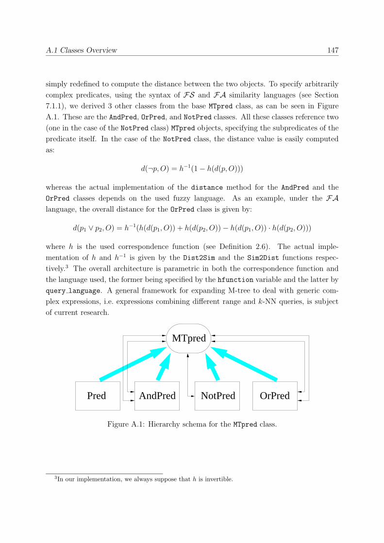
A.1 Classes Overview 147
simply redefined to compute the distance between the two objects. To specify arbitrarily
complex predicates, using the syntax of FS and FA similarity languages (see Section
7.1.1), we derived 3 other classes from the base MTpred class, as can be seen in Figure
A.1. These are the AndPred, OrPred, and NotPred classes. All these classes reference two
(one in the case of the NotPred class) MTpred objects, specifying the subpredicates of the
predicate itself. In the case of the NotPred class, the distance value is easily computed
as:
d(¬p,O) = h−1(1− h(d(p,O)))
whereas the actual implementation of the distance method for the AndPred and the
OrPred classes depends on the used fuzzy language. As an example, under the FAlanguage, the overall distance for the OrPred class is given by:
d(p1 ∨ p2, O) = h−1(h(d(p1, O)) + h(d(p2, O))− h(d(p1, O)) · h(d(p2, O)))
where h is the used correspondence function (see Definition 2.6). The actual imple-
mentation of h and h−1 is given by the Dist2Sim and the Sim2Dist functions respec-
tively.3 The overall architecture is parametric in both the correspondence function and
the language used, the former being specified by the hfunction variable and the latter by
query language. A general framework for expanding M-tree to deal with generic com-
plex expressions, i.e. expressions combining different range and k-NN queries, is subject
of current research.
MTpred
Pred AndPred NotPred OrPred
Figure A.1: Hierarchy schema for the MTpred class.
3In our implementation, we always suppose that h is invertible.

Appendix B
The Colors Application
In this Chapter we introduce a prototype application that demonstrate the effectiveness of
the similarity search techniques developed in this thesis on a real-world problem, namely
the content-based retrieval of images by means of color features.
The main objective of the Colors prototype is to show both the generality and the
power of the approach presented in Chapter 7 for the optimization of complex content ori-
ented requests. The software architecture, being parametric in the similarity environment
(see Definition 7.4), could be, in principle, applied to a generic distance-based scenario,
but we chose the image retrieval environment for its immediate visual impact.
B.1 Defining the Similarity Environment
The dataset used in the Colors application consists of 11,650 real-color JPEG compressed
[Wal91] thumbnails of size 180x120 pixels. The used distance function is that defined
in [SO95], where the average, variance and skewness of hue, saturation, and brightness
components are extracted for each image, and a weighted L1 metric is used to compare the
9-dimensional feature vectors. It should be noted that the evaluation of the effectiveness
of the similarity function is definitely out of the scope of the application. The same
approach can be used with any similarity function used to compare images, possibly
including texture and/or spatial information.
Feature vectors extracted from the images were indexed using an M-tree, obtaining an
index consisting of 632 pages of 4 Kbytes arranged on 3 levels. A sequential file of feature
vectors was also created, consisting of 219 pages.
149
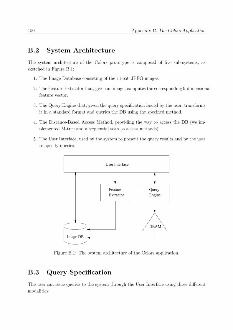
150 Appendix B. The Colors Application
B.2 System Architecture
The system architecture of the Colors prototype is composed of five sub-systems, as
sketched in Figure B.1:
1. The Image Database consisting of the 11,650 JPEG images.
2. The Feature Extractor that, given an image, computes the corresponding 9-dimensional
feature vector.
3. The Query Engine that, given the query specification issued by the user, transforms
it in a standard format and queries the DB using the specified method.
4. The Distance-Based Access Method, providing the way to access the DB (we im-
plemented M-tree and a sequential scan as access methods).
5. The User Interface, used by the system to present the query results and by the user
to specify queries.
User Interface
QueryEngine
FeatureExtractor
DBAM
Image DB
Figure B.1: The system architecture of the Colors application.
B.3 Query Specification
The user can issue queries to the system through the User Interface using three different
modalities:
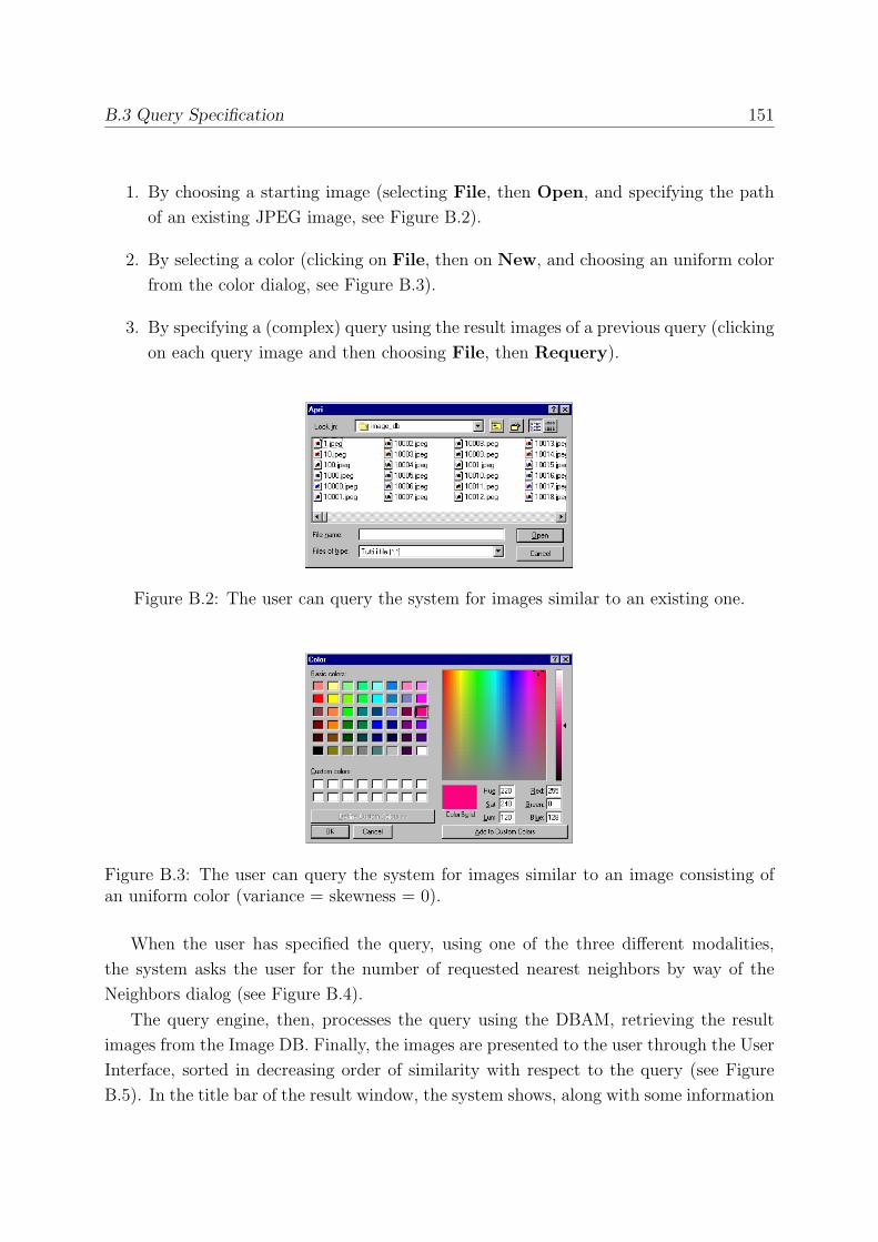
B.3 Query Specification 151
1. By choosing a starting image (selecting File, then Open, and specifying the path
of an existing JPEG image, see Figure B.2).
2. By selecting a color (clicking on File, then on New, and choosing an uniform color
from the color dialog, see Figure B.3).
3. By specifying a (complex) query using the result images of a previous query (clicking
on each query image and then choosing File, then Requery).
Figure B.2: The user can query the system for images similar to an existing one.
Figure B.3: The user can query the system for images similar to an image consisting ofan uniform color (variance = skewness = 0).
When the user has specified the query, using one of the three different modalities,
the system asks the user for the number of requested nearest neighbors by way of the
Neighbors dialog (see Figure B.4).
The query engine, then, processes the query using the DBAM, retrieving the result
images from the Image DB. Finally, the images are presented to the user through the User
Interface, sorted in decreasing order of similarity with respect to the query (see Figure
B.5). In the title bar of the result window, the system shows, along with some information

152 Appendix B. The Colors Application
Figure B.4: The Neighbors dialog.
Figure B.5: The result of a query.
about the search method and the used similarity environment, the number of computed
distances and of page I/Os (for a page size of 4 Kbytes).
When the user issues a complex query using the result of a previous one, he can specify
both positive and negative examples. Positive examples are selected by clicking on the
image; the system shows a blue frame around the image and the predicate is conjuncted
to the query using an and operator. Negative examples are selected by clicking on the
image with the Ctrl key pressed; the system shows a red frame around the image and the
predicate is conjuncted to the query using and not. Figure B.6 show an example of a
query; in this case two positive and one negative examples are specified.
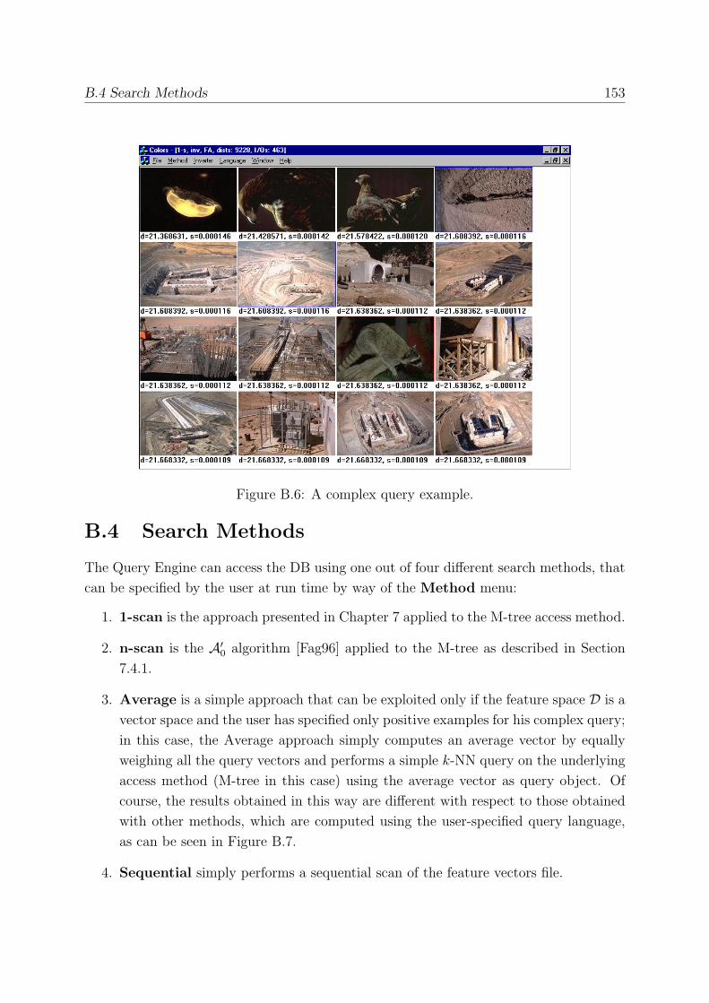
B.4 Search Methods 153
Figure B.6: A complex query example.
B.4 Search Methods
The Query Engine can access the DB using one out of four different search methods, that
can be specified by the user at run time by way of the Method menu:
1. 1-scan is the approach presented in Chapter 7 applied to the M-tree access method.
2. n-scan is the A′0 algorithm [Fag96] applied to the M-tree as described in Section
7.4.1.
3. Average is a simple approach that can be exploited only if the feature space D is avector space and the user has specified only positive examples for his complex query;
in this case, the Average approach simply computes an average vector by equally
weighing all the query vectors and performs a simple k-NN query on the underlying
access method (M-tree in this case) using the average vector as query object. Of
course, the results obtained in this way are different with respect to those obtained
with other methods, which are computed using the user-specified query language,
as can be seen in Figure B.7.
4. Sequential simply performs a sequential scan of the feature vectors file.
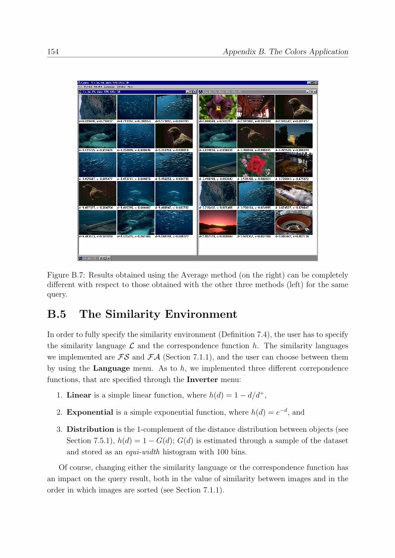
154 Appendix B. The Colors Application
Figure B.7: Results obtained using the Average method (on the right) can be completelydifferent with respect to those obtained with the other three methods (left) for the samequery.
B.5 The Similarity Environment
In order to fully specify the similarity environment (Definition 7.4), the user has to specify
the similarity language L and the correspondence function h. The similarity languages
we implemented are FS and FA (Section 7.1.1), and the user can choose between them
by using the Language menu. As to h, we implemented three different correpondence
functions, that are specified through the Inverter menu:
1. Linear is a simple linear function, where h(d) = 1− d/d+,
2. Exponential is a simple exponential function, where h(d) = e−d, and
3. Distribution is the 1-complement of the distance distribution between objects (see
Section 7.5.1), h(d) = 1−G(d); G(d) is estimated through a sample of the dataset
and stored as an equi-width histogram with 100 bins.
Of course, changing either the similarity language or the correspondence function has
an impact on the query result, both in the value of similarity between images and in the
order in which images are sorted (see Section 7.1.1).
Bibliography
[AMN+94] Sunil Arya, David M. Mount, Nathan S. Netanyahu, Ruth Silverman, and
Angela Y. Wu. An optimal algorithm for approximate nearest neighbor
searching. In Proceedings of the 5th Annual ACM-SIAM Symposium on Dis-
crete Algorithms, pages 573–582, Arlington, VA, January 1994.
[BBK98] Stefan Berchtold, Christian Bohm, and Hans-Peter Kriegel. The pyramid-
technique: Towards breaking the curse of dimensionality. In Proceedings of
the 1998 ACM SIGMOD International Conference on Management of Data,
pages 142–153, Seattle, WA, June 1998.
[BBKK97] Stefan Berchtold, Christian Bohm, Daniel A. Keim, and Hans-Peter Kriegel.
A cost model for nearest neighbor search in high-dimensional data space.
In Proceedings of the 16th ACM SIGACT-SIGMOD-SIGART Symposium on
Principles of Database Systems (PODS’97), pages 78–86, Tucson, AZ, May
1997.
[BFM+96] Julio Barros, James French, Worthy Martin, Patrick Kelly, and Mike Can-
non. Using the triangle inequality to reduce the number of comparisons re-
quired for similarity-based retrieval. In Electronic Imaging ’96, Storage and
Retrieval for Still Image and Video Databases IV, San Jose, CA, January
1996.
[BKK96] Stefan Berchtold, Daniel A. Keim, and Hans-Peter Kriegel. The X-tree:
An index structure for high-dimensional data. In Proceedings of the 22nd
International Conference on Very Large Data Bases (VLDB’96), pages 28–
39, Mumbai (Bombay), India, September 1996.
[BKSS90] Norbert Beckmann, Hans-Peter Kriegel, Ralf Schneider, and Bernhard
Seeger. The R∗-tree: An efficient and robust access method for points andrectangles. In Proceedings of the 1990 ACM SIGMOD International Confer-
ence on Management of Data, pages 322–331, Atlantic City, NJ, May 1990.
155
156 Bibliography
[BO97] Tolga Bozkaya and Meral Ozsoyoglu. Distance-based indexing for high-
dimensional metric spaces. In Proceedings of the 1997 ACM SIGMOD Inter-
national Conference on Management of Data, pages 357–368, Tucson, AZ,
May 1997.
[BP93] Roberto Brunelli and Tomaso Poggio. Face recognition: Features versus
templates. IEEE Transactions on Pattern Analysis and Machine Intelligence,
15(10):1042–1052, 1993.
[Bri95] Sergey Brin. Near neighbor search in large metric spaces. In Proceedings
of the 21st International Conference on Very Large Data Bases (VLDB’95),
pages 574–584, Zurich, Switzerland, September 1995.
[BYO97] Tolga Bozkaya, Nasser Yazdani, and Meral Ozsoyoglu. Matching and index-
ing sequences of different lengths. In Proceedings of the 6th International
Conference on Information and Knowledge Management (CIKM’97), pages
128–135, Las Vegas, NE, November 1997.
[CA97] Weimin Chen and Karl Aberer. Efficient querying on genomic databases by
using metric space indexing techniques. In 1st International Workshop on
Query Processing and Multimedia Issues in Distributed Systems (PMIDS’97),
Toulouse, France, September 1997.
[CG96] Surajit Chaudhuri and Luis Gravano. Optimizing queries over multimedia
repositories. In Proceedings 1996 ACM SIGMOD International Conference
on Management of Data, pages 91–102, Montreal, Canada, June 1996.
[Chi94] Tzi-cker Chiueh. Content-based image indexing. In Proceedings of the 20th
International Conference on Very Large Data Bases (VLDB’94), pages 582–
593, Santiago, Chile, September 1994.
[Cia98] Paolo Ciaccia. An algebra for similarity queries and its index-based evalu-
ation. Technical report, ESPRIT LTR Project HERMES (no. 9141), 1998.
Available at URL http://www.ced.tuc.gr/hermes/.
[CNP99] Paolo Ciaccia, Alessandro Nanni, and Marco Patella. A query-sensitive
cost model for similarity queries with M-tree. In Proceedings of the 10th
Australasian Database Conference (ADC’99), pages 65–76, Auckland, New
Zealand, January 1999.
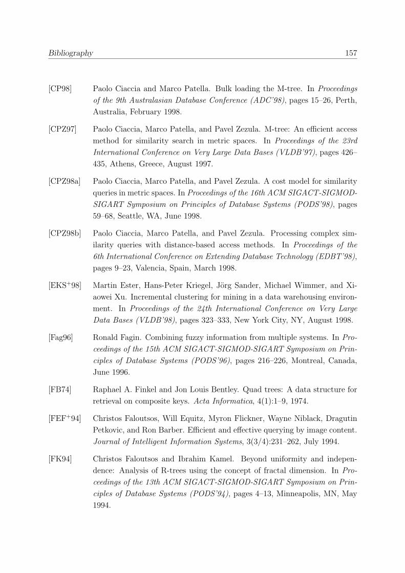
Bibliography 157
[CP98] Paolo Ciaccia and Marco Patella. Bulk loading the M-tree. In Proceedings
of the 9th Australasian Database Conference (ADC’98), pages 15–26, Perth,
Australia, February 1998.
[CPZ97] Paolo Ciaccia, Marco Patella, and Pavel Zezula. M-tree: An efficient access
method for similarity search in metric spaces. In Proceedings of the 23rd
International Conference on Very Large Data Bases (VLDB’97), pages 426–
435, Athens, Greece, August 1997.
[CPZ98a] Paolo Ciaccia, Marco Patella, and Pavel Zezula. A cost model for similarity
queries in metric spaces. In Proceedings of the 16th ACM SIGACT-SIGMOD-
SIGART Symposium on Principles of Database Systems (PODS’98), pages
59–68, Seattle, WA, June 1998.
[CPZ98b] Paolo Ciaccia, Marco Patella, and Pavel Zezula. Processing complex sim-
ilarity queries with distance-based access methods. In Proceedings of the
6th International Conference on Extending Database Technology (EDBT’98),
pages 9–23, Valencia, Spain, March 1998.
[EKS+98] Martin Ester, Hans-Peter Kriegel, Jorg Sander, Michael Wimmer, and Xi-
aowei Xu. Incremental clustering for mining in a data warehousing environ-
ment. In Proceedings of the 24th International Conference on Very Large
Data Bases (VLDB’98), pages 323–333, New York City, NY, August 1998.
[Fag96] Ronald Fagin. Combining fuzzy information from multiple systems. In Pro-
ceedings of the 15th ACM SIGACT-SIGMOD-SIGART Symposium on Prin-
ciples of Database Systems (PODS’96), pages 216–226, Montreal, Canada,
June 1996.
[FB74] Raphael A. Finkel and Jon Louis Bentley. Quad trees: A data structure for
retrieval on composite keys. Acta Informatica, 4(1):1–9, 1974.
[FEF+94] Christos Faloutsos, Will Equitz, Myron Flickner, Wayne Niblack, Dragutin
Petkovic, and Ron Barber. Efficient and effective querying by image content.
Journal of Intelligent Information Systems, 3(3/4):231–262, July 1994.
[FK94] Christos Faloutsos and Ibrahim Kamel. Beyond uniformity and indepen-
dence: Analysis of R-trees using the concept of fractal dimension. In Pro-
ceedings of the 13th ACM SIGACT-SIGMOD-SIGART Symposium on Prin-
ciples of Database Systems (PODS’94), pages 4–13, Minneapolis, MN, May
1994.
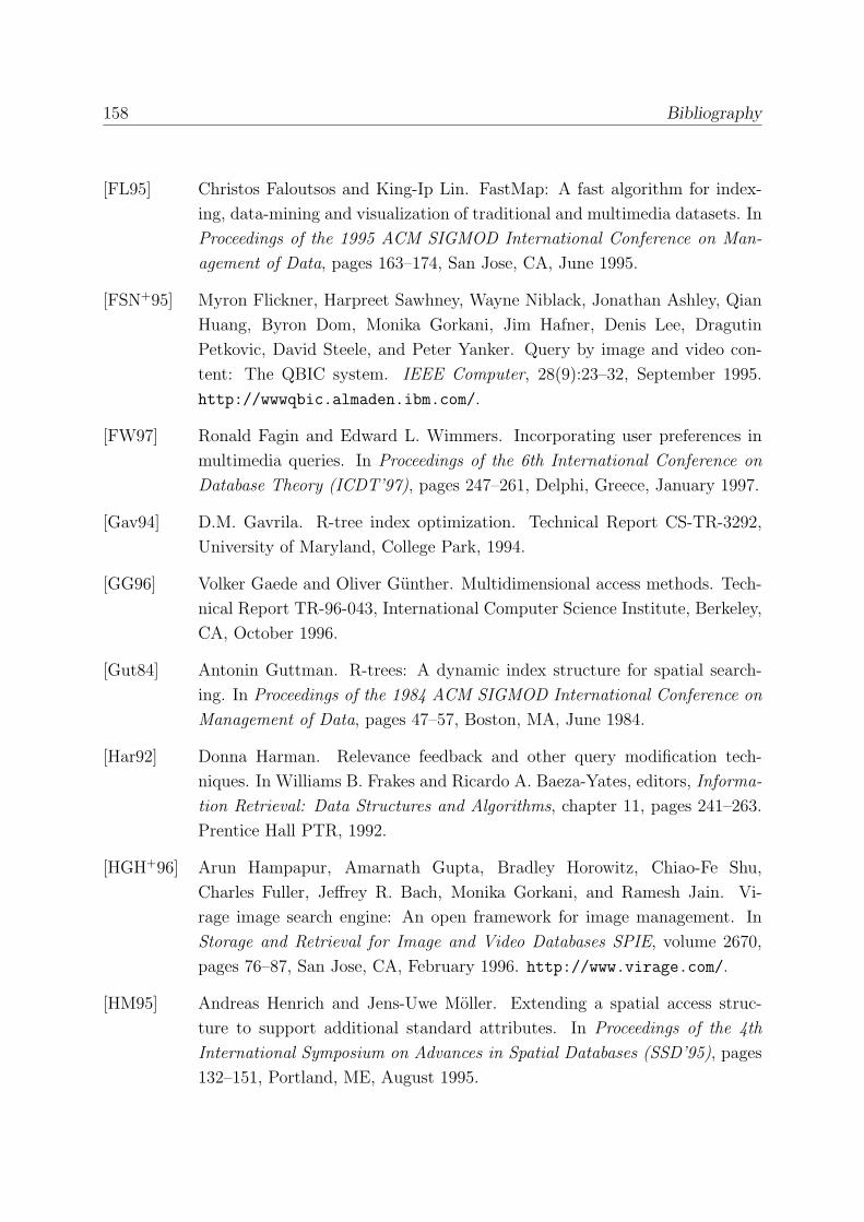
158 Bibliography
[FL95] Christos Faloutsos and King-Ip Lin. FastMap: A fast algorithm for index-
ing, data-mining and visualization of traditional and multimedia datasets. In
Proceedings of the 1995 ACM SIGMOD International Conference on Man-
agement of Data, pages 163–174, San Jose, CA, June 1995.
[FSN+95] Myron Flickner, Harpreet Sawhney, Wayne Niblack, Jonathan Ashley, Qian
Huang, Byron Dom, Monika Gorkani, Jim Hafner, Denis Lee, Dragutin
Petkovic, David Steele, and Peter Yanker. Query by image and video con-
tent: The QBIC system. IEEE Computer, 28(9):23–32, September 1995.
http://wwwqbic.almaden.ibm.com/.
[FW97] Ronald Fagin and Edward L. Wimmers. Incorporating user preferences in
multimedia queries. In Proceedings of the 6th International Conference on
Database Theory (ICDT’97), pages 247–261, Delphi, Greece, January 1997.
[Gav94] D.M. Gavrila. R-tree index optimization. Technical Report CS-TR-3292,
University of Maryland, College Park, 1994.
[GG96] Volker Gaede and Oliver Gunther. Multidimensional access methods. Tech-
nical Report TR-96-043, International Computer Science Institute, Berkeley,
CA, October 1996.
[Gut84] Antonin Guttman. R-trees: A dynamic index structure for spatial search-
ing. In Proceedings of the 1984 ACM SIGMOD International Conference on
Management of Data, pages 47–57, Boston, MA, June 1984.
[Har92] Donna Harman. Relevance feedback and other query modification tech-
niques. In Williams B. Frakes and Ricardo A. Baeza-Yates, editors, Informa-
tion Retrieval: Data Structures and Algorithms, chapter 11, pages 241–263.
Prentice Hall PTR, 1992.
[HGH+96] Arun Hampapur, Amarnath Gupta, Bradley Horowitz, Chiao-Fe Shu,
Charles Fuller, Jeffrey R. Bach, Monika Gorkani, and Ramesh Jain. Vi-
rage image search engine: An open framework for image management. In
Storage and Retrieval for Image and Video Databases SPIE, volume 2670,
pages 76–87, San Jose, CA, February 1996. http://www.virage.com/.
[HM95] Andreas Henrich and Jens-Uwe Moller. Extending a spatial access struc-
ture to support additional standard attributes. In Proceedings of the 4th
International Symposium on Advances in Spatial Databases (SSD’95), pages
132–151, Portland, ME, August 1995.
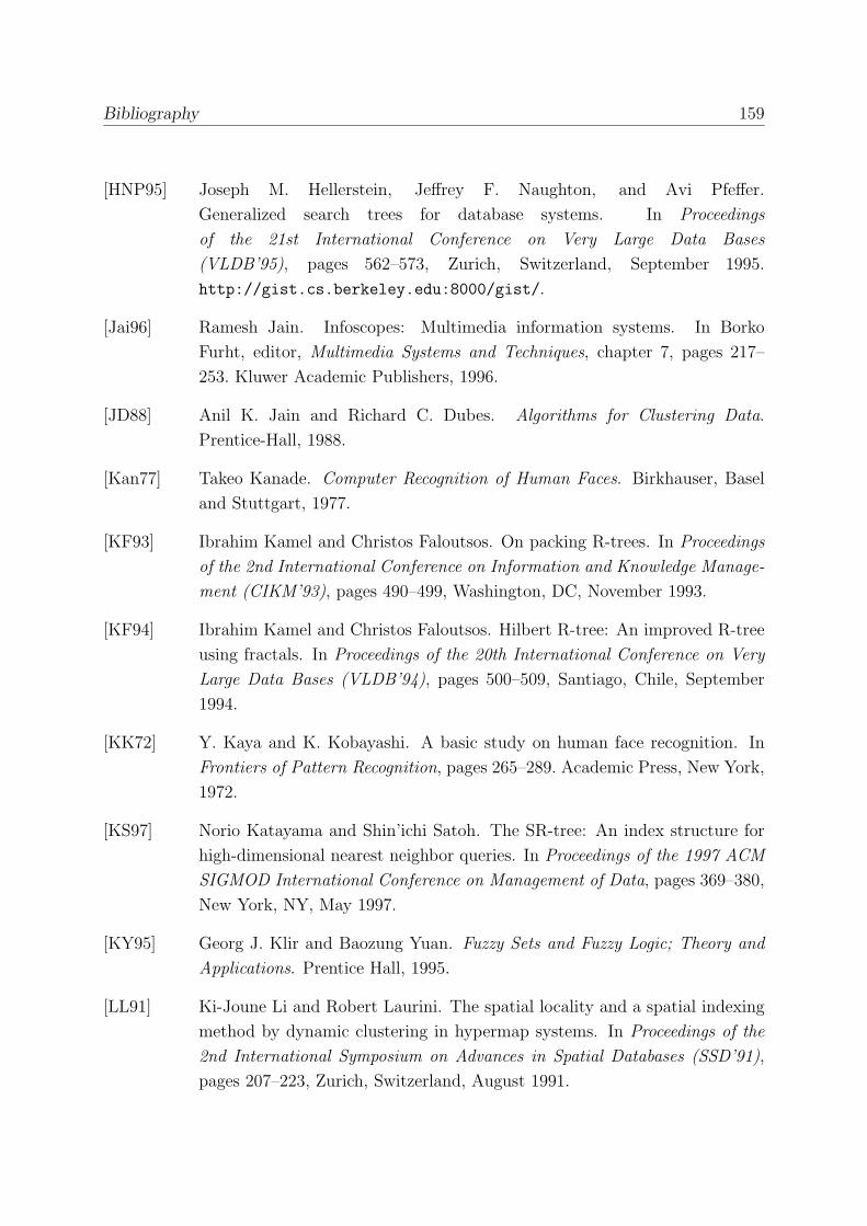
Bibliography 159
[HNP95] Joseph M. Hellerstein, Jeffrey F. Naughton, and Avi Pfeffer.
Generalized search trees for database systems. In Proceedings
of the 21st International Conference on Very Large Data Bases
(VLDB’95), pages 562–573, Zurich, Switzerland, September 1995.
http://gist.cs.berkeley.edu:8000/gist/.
[Jai96] Ramesh Jain. Infoscopes: Multimedia information systems. In Borko
Furht, editor, Multimedia Systems and Techniques, chapter 7, pages 217–
253. Kluwer Academic Publishers, 1996.
[JD88] Anil K. Jain and Richard C. Dubes. Algorithms for Clustering Data.
Prentice-Hall, 1988.
[Kan77] Takeo Kanade. Computer Recognition of Human Faces. Birkhauser, Basel
and Stuttgart, 1977.
[KF93] Ibrahim Kamel and Christos Faloutsos. On packing R-trees. In Proceedings
of the 2nd International Conference on Information and Knowledge Manage-
ment (CIKM’93), pages 490–499, Washington, DC, November 1993.
[KF94] Ibrahim Kamel and Christos Faloutsos. Hilbert R-tree: An improved R-tree
using fractals. In Proceedings of the 20th International Conference on Very
Large Data Bases (VLDB’94), pages 500–509, Santiago, Chile, September
1994.
[KK72] Y. Kaya and K. Kobayashi. A basic study on human face recognition. In
Frontiers of Pattern Recognition, pages 265–289. Academic Press, New York,
1972.
[KS97] Norio Katayama and Shin’ichi Satoh. The SR-tree: An index structure for
high-dimensional nearest neighbor queries. In Proceedings of the 1997 ACM
SIGMOD International Conference on Management of Data, pages 369–380,
New York, NY, May 1997.
[KY95] Georg J. Klir and Baozung Yuan. Fuzzy Sets and Fuzzy Logic; Theory and
Applications. Prentice Hall, 1995.
[LL91] Ki-Joune Li and Robert Laurini. The spatial locality and a spatial indexing
method by dynamic clustering in hypermap systems. In Proceedings of the
2nd International Symposium on Advances in Spatial Databases (SSD’91),
pages 207–223, Zurich, Switzerland, August 1991.
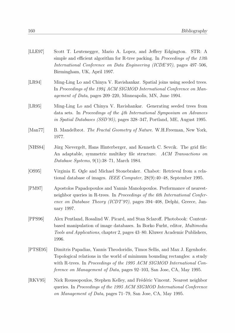
160 Bibliography
[LLE97] Scott T. Leutenegger, Mario A. Lopez, and Jeffrey Edgington. STR: A
simple and efficient algorithm for R-tree packing. In Proceedings of the 13th
International Conference on Data Engineering (ICDE’97), pages 497–506,
Birmingham, UK, April 1997.
[LR94] Ming-Ling Lo and Chinya V. Ravishankar. Spatial joins using seeded trees.
In Proceedings of the 1994 ACM SIGMOD International Conference on Man-
agement of Data, pages 209–220, Minneapolis, MN, June 1994.
[LR95] Ming-Ling Lo and Chinya V. Ravishankar. Generating seeded trees from
data sets. In Proceedings of the 4th International Symposium on Advances
in Spatial Databases (SSD’95), pages 328–347, Portland, ME, August 1995.
[Man77] B. Mandelbrot. The Fractal Geometry of Nature. W.H.Freeman, New York,
1977.
[NHS84] Jurg Nievergelt, Hans Hinterberger, and Kenneth C. Sevcik. The grid file:
An adaptable, symmetric multikey file structure. ACM Transactions on
Database Systems, 9(1):38–71, March 1984.
[OS95] Virginia E. Ogle and Michael Stonebraker. Chabot: Retrieval from a rela-
tional database of images. IEEE Computer, 28(9):40–48, September 1995.
[PM97] Apostolos Papadopoulos and Yannis Manolopoulos. Performance of nearest-
neighbor queries in R-trees. In Proceedings of the 6th International Confer-
ence on Database Theory (ICDT’97), pages 394–408, Delphi, Greece, Jan-
uary 1997.
[PPS96] Alex Pentland, Rosalind W. Picard, and Stan Sclaroff. Photobook: Content-
based manipulation of image databases. In Borko Furht, editor, Multimedia
Tools and Applications, chapter 2, pages 43–80. Kluwer Academic Publishers,
1996.
[PTSE95] Dimitris Papadias, Yannis Theodoridis, Timos Sellis, and Max J. Egenhofer.
Topological relations in the world of minimum bounding rectangles: a study
with R-trees. In Proceedings of the 1995 ACM SIGMOD International Con-
ference on Management of Data, pages 92–103, San Jose, CA, May 1995.
[RKV95] Nick Roussopoulos, Stephen Kelley, and Frederic Vincent. Nearest neighbor
queries. In Proceedings of the 1995 ACM SIGMOD International Conference
on Management of Data, pages 71–79, San Jose, CA, May 1995.
Bibliography 161
[RL85] Nick Roussopoulos and Daniel Leifker. Direct spatial search on pictorial
databases using packed R-trees. In Proceedings of the 1985 ACM SIGMOD
International Conference on Management of Data, pages 17–31, Austin, TX,
May 1985.
[Sam89] Hanan Samet. The Design and Analysis of Spatial Data Structures. Addison-
Wesley, Redding, MA, 1989.
[SC96] John R. Smith and Shih-Fu Chang. VisualSEEk: A fully automated
content-based image query system. In Proceedings of the 4th ACM Inter-
national Conference on Multimedia, pages 87–98, Boston, MA, November
1996. http://www.ctr.columbia.edu/visualseek/.
[Sco92] David W. Scott. Multivariate Density Estimation. Theory, Practice and
Visualization. Wiley-Interscience, New York, 1992.
[Sha77] Marvin Shapiro. The choice of reference points in best-match file searching.
Communications of the ACM, 20(5):339–343, 1977.
[SJ98] Simone Santini and Ramesh Jain. Similarity matching. To appear in IEEE
Transactions on Pattern Analysis and Machine Intelligence, 1998.
[SK88] Bernhard Seeger and Hans-Peter Kriegel. Techniques for design and im-
plementation of efficient spatial access methods. In Proceedings of the 14th
International Conference on Very Large Data Bases (VLDB’88), pages 360–
371, Los Angeles, CA, August 1988.
[SK97] Thomas Seidl and Hans-Peter Kriegel. Efficient user-adaptable similarity
search in large multimedia databases. In Proceedings of the 23rd International
Conference on Very Large Data Bases (VLDB’97), pages 506–515, Athens,
Greece, August 1997.
[SK98] Thomas Seidl and Hans-Peter Kriegel. Optimal multi-step k-nearest neighbor
search. In Proceedings of the 1998 ACM SIGMOD International Conference
on Management of Data, pages 154–165, Seattle, WA, June 1998.
[Smi97] John R. Smith. Integrated Spatial and Feature Image Systems: Retrieval,
Analysis and Compression. PhD thesis, Columbia University, 1997.
[SO95] Markus Stricker and Markus Orengo. Similarity of color images. In Storage
and Retrieval for Image and Video Databases SPIE, volume 2420, pages 381–
392, San Jose, CA, February 1995.

162 Bibliography
[SRF87] Timos Sellis, Nick Roussopoulos, and Christos Faloutsos. The R+-tree: A
dynamic index for multi-dimensional objects. In Proceedings of the 13th
International Conference on Very Large Data Bases (VLDB’87), pages 507–
518, Brighton, England, September 1987.
[SZ+96] Avi Silberschatz, Stan Zdonik, et al. Strategic directions in database sys-
tems — breaking out of the box. ACM Computing Surveys, 28(4):764–778,
December 1996.
[TP91] Matthew Turk and Alex Pentland. Eigenfaces for recognition. Journal of
Cognitive Neuroscience, 3(1):71–87, 1991.
[TS96] Yannis Theodoridis and Timos Sellis. A model for the prediction of R-tree
performance. In Proceedings of the 15th ACM SIGACT-SIGMOD-SIGART
Symposium on Principles of Database Systems (PODS’96), pages 161–171,
Montreal, Canada, June 1996.
[Uhl91] Jeffrey K. Uhlmann. Satisfying general proximity/similarity queries with
metric trees. Information Processing Letters, 40(4):175–179, November 1991.
[vdBSW97] Jochen van den Bercken, Bernhard Seeger, and Peter Widmayer. A generic
approach to bulk loading multidimensional index structures. In Proceedings
of the 23rd International Conference on Very Large Data Bases (VLDB’97),
pages 406–415, Athens, Greece, August 1997.
[Wal91] Gregory K. Wallace. The JPEG still picture compression standard. Com-
munications of the ACM, 34(4):30–44, April 1991.
[WBKW96] Erling Wold, Thom Blum, Douglas Keislar, and James Wheaton. Content-
based classification, search, and retrieval of audio. IEEE Multimedia,
3(3):27–36, 1996.
[WJ96] David A. White and Ramesh Jain. Similarity indexing with the SS-tree.
In Proceedings of the 12th International Conference on Data Engineering
(ICDE’96), pages 516–523, New Orleans, LO, February 1996.
[WSB98] Roger Weber, Hans-Jorg Schek, and Stephen Blott. A quantitative analysis
and performance study for similarity-search methods in high-dimensional
spaces. In Proceedings of the 24th International Conference on Very Large
Data Bases (VLDB’98), pages 194–205, New York, NY, August 1998.
Bibliography 163
[WZ96] HughWilliams and Justin Zobel. Indexing nucleotide databases for fast query
evaluation. In Proceedings of the 5th International Conference on Extending
Database Technology (EDBT’96), pages 275–288, Avignon, France, March
1996.
[Yia93] Peter N. Yianilos. Data structures and algorithms for nearest neighbor search
in general metric spaces. In Proceedings of the 4th ACM-SIAM Symposium
on Discrete Algorithms (SODA’93), pages 311–321, Austin, TX, January
1993.
[Zad65] Lotfi Asker Zadeh. Fuzzy sets. Information and Control, 8:338–353, 1965.
[ZCF+97] Carlo Zaniolo, Stefano Ceri, Christos Faloutsos, Richard T. Snodgrass, V.S.
Subrahmanian, and Roberto Zicari, editors. Advanced Database Systems.
Morgan Kaufmann, San Francisco, 1997.
[ZSAR98] Pavel Zezula, Pasquale Savino, Giuseppe Amato, and Fausto Rabitti. Ap-
proximate similarity retrieval with M-trees. The VLDB Journal, 7(4):275–
293, 1998.


“In my end is my beginning”
Thomas Stearn Eliot