Embed Size (px)
Citation preview

UNIVERSITÀ DEGLI STUDI DI SIENA
QUADERNI DEL DIPARTIMENTO
DI ECONOMIA POLITICA E STATISTICA
Pierpaolo Pierani Silvia Tiezzi
Revealed Bounded rationality:
Testing present bias in a Rational Addiction Equation
n. 666 – Dicembre 2012
ABSTRACT - This paper deals with one of the main theoretical and empirical problems associated with the rational addiction model, namely that the demand equation derived from the rational addiction theory is not empirically distinguishable from models with forward‐looking behavior, but with timeinconsistent preferences. The implication is that, even when forward‐looking behavior can be convincingly supported, this equation cannot provide evidence in favor of time‐consistent preferences against a model with dynamic inconsistency. In fact, we show that the possibility of testing for exponential versus non‐exponential time discounting is nested within the rational addiction model. We propose a test of time consistency that uses only the information obtained from the general rational addiction demand equation and the price effects. A pseudo panel of Italian households is used to test for rational addiction in tobacco consumption. GMM estimators are used to deal with errors in variables and unobserved heterogeneity. The results conform to the theoretical predictions. We find evidence that tobacco consumers are forward‐looking, but timeinconsistent. The values of the derived present bias and long run discount parameters are statistically significant and in line with the literature. JEL codes: C23, D03, D12 Keywords: rational addiction, time inconsistency, GMM.
Pierpaolo Pierani Department of Economics and Statistics, University of Siena, Siena, IT 53100, EU,
Silvia Tiezzi Department of Economics and Statistics, University of Siena, Siena, IT 53100, EU, and
Visiting Professor, Department of Social and Decision Sciences, Carnegie Mellon University, Pittsburgh, PA 15213, USA, [email protected]
1
1. INTRODUCTION
Becker and Murphy (1988) explored the dynamic behavior of the consumption of addictive goods,
pointing out that many phenomena previously thought to be irrational are in fact consistent with
optimization according to stable preferences. In their model, individuals recognize both the
current and the future consequences of consuming addictive goods. This model of rational
addiction has subsequently become the standard approach to modeling consumption of goods
such as cigarettes. A sizable empirical literature has been developed since then, beginning with
Becker, Grossman and Murphy (1994), which has tested and generally supported the empirical
predictions of the Becker and Murphy model. These past contributions, however, run into a
number of critical drawbacks.
This paper is concerned with one of these problems, namely that forward‐looking behavior,
implied by the model, does not necessarily mean time consistency. More precisely, the equation
derived from the theory is not empirically distinguishable from models with forward‐looking
behavior, but with time‐inconsistent preferences. So, forward‐looking behavior does not provide
evidence in favor of time‐consistent preferences against a model with dynamic inconsistency
(Gruber and Köszegi, 2000).
This is a crucial issue, because models with dynamic inconsistency can deliver radically different
implications for government policy. In particular, while the rational addiction model implies that
the optimal tax on addictive goods should depend only on the externalities that their use imposes
on society, the time‐inconsistent alternative suggests a much higher tax depending also on the
“internalities” that drugs’ use imposes on consumers. In modeling and testing for addiction, it is
therefore very important to distinguish between time‐consistent and time‐inconsistent agents.
The early literature on dynamic consumption behavior modeled impatience in decision making by
assuming that agents discount future streams of utility or profits exponentially over time.
Exponential discounting is pivotal. Without this assumption, inter‐temporal marginal rates of
substitution will change as time passes, and preferences will be time‐inconsistent (Strotz, 1956).
Recently, behavioral economics literature has built on the work of Strotz (1956), to explore the
consequences of relaxing the standard assumption of exponential discounting. Ainslie (1992) and
Loewenstein and Elster (1992) indicate that hyperbolic discounting may explain some basic
features of inter‐temporal decision‐making that are inconsistent with simple models of
exponential discounting, namely that hyperbolic discounters value consumption in the present
more than any delayed consumption. In the formulation of quasi‐hyperbolic discounting adopted
by Laibson (1997), the degree of present bias is captured by an extra discount parameter 1, which captures the taste for instant gratification1. The consequence of quasi‐hyperbolic
discounting is that the discount factor between two consecutive future periods ( ) is larger than 1The "quasi-hyperbolic" discount function approximates the hyperbolic discount function in discrete time taking β and as constants between 0 and 1.
2
that between today and tomorrow ( ). O’Donoghue and Rabin (2002) and Gruber and Köszegi
(2001) show that present bias can lead individuals to greatly over‐consume the addictive good,
with the consequence of a substantial welfare loss.
The implications of time‐inconsistent preferences, and their associated problems of self‐control,
have been studied under a variety of economic choices and environments. Laibson (1997),
O’Donoghue and Rabin (1999a; b) and Angeletos et al. (2001) applied this formulation to
consumption and saving behavior; Diamond and Köszegi (1998) explored retirement decisions;
Barro (1999) applied it to growth; Gruber and Köszegi (2001), Ciccarelli, Giamboni and Waldmann
(2008) and Levy (2010) to smoking behavior; Shapiro (2005) to caloric intake; Fang and Silverman
(2009) to welfare program participation and labor supply of single mothers with dependent
children; Della Vigna and Paserman (2005) to job search (see Della Vigna 2009 for a review) and
Acland and Levy (2010) to gym attendance.
Despite this booming of interest, estimates of the short‐run discount factor and tests of present bias using observational rather than experimental data are still scarce. Few recent works have attempted to use a parametric approach to estimate structural dynamic models with hyperbolic time preferences (Fang and Silverman, 2009; Laibson, Repetto and Tobacman, 2007; Paserman, 2008). Focusing on addictive goods, Levy (2010) derives estimates of the degree of present bias using a model of cigarette addiction based on O’Donoghue and Rabin’s (2002) generalization of Becker and Murphy’s (1988) rational addiction model. Gruber and Koszegi (2001) develop a new model of addictive behavior that takes as its starting point the standard rational addiction model, but incorporates quasi‐hyperbolic discounting preferences. They propose using information extracted from their model to obtain the present bias and long‐run discounting parameters and, in a previous version of the same paper, they also propose a test of time consistency per se. In practice, however, they were unable to carry out this test and to back out the two discount parameters. Ciccarelli, Giamboni and Waldmann (2008) tested for time preferences by exploring smoking by women before, during and after pregnancy using the European Community Household Panel (ECHP). Their specification does not match the original rational addiction demand equation. Rather, they use a modified specification with several lead consumption terms and make inferences about the time preferences of the underlying actors based on the assumption that, if preferences are time‐consistent, smoking at t+1 is a sufficient statistic for the whole stream of future smoking, i.e., expected smoking more than one period ahead should have no independent effect on smoking. To our best knowledge no research has been developed to date to test the assumption of instant gratification within the structural demand equation derived from the rational addiction model.
This paper makes three distinct contributions to the literature on addiction and time preferences.
First, it provides an estimate, using pseudo panel data at the individual level, of the general
specification of the rational addiction demand equation that includes past and future prices. As far
as we know this formulation has been estimated only twice before, by Becker, Grossman and
3
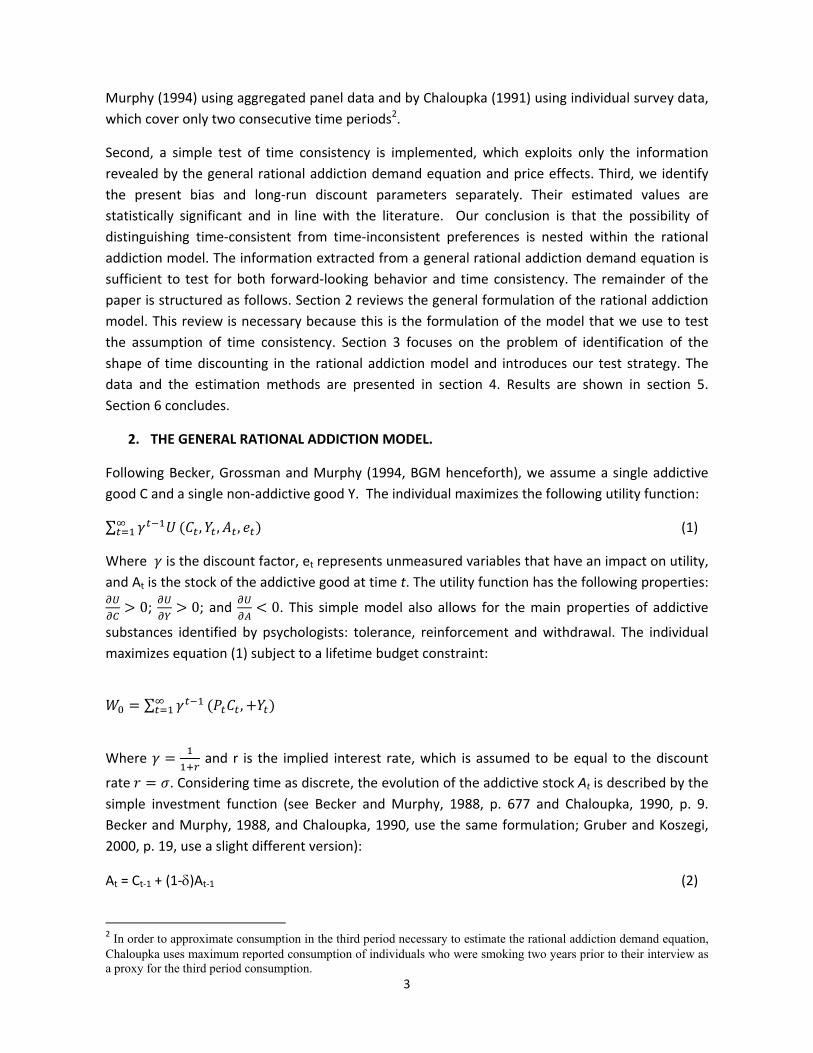
Murphy (1994) using aggregated panel data and by Chaloupka (1991) using individual survey data,
which cover only two consecutive time periods2.
Second, a simple test of time consistency is implemented, which exploits only the information
revealed by the general rational addiction demand equation and price effects. Third, we identify
the present bias and long‐run discount parameters separately. Their estimated values are
statistically significant and in line with the literature. Our conclusion is that the possibility of
distinguishing time‐consistent from time‐inconsistent preferences is nested within the rational
addiction model. The information extracted from a general rational addiction demand equation is
sufficient to test for both forward‐looking behavior and time consistency. The remainder of the
paper is structured as follows. Section 2 reviews the general formulation of the rational addiction
model. This review is necessary because this is the formulation of the model that we use to test
the assumption of time consistency. Section 3 focuses on the problem of identification of the
shape of time discounting in the rational addiction model and introduces our test strategy. The
data and the estimation methods are presented in section 4. Results are shown in section 5.
Section 6 concludes.
2. THE GENERAL RATIONAL ADDICTION MODEL.
Following Becker, Grossman and Murphy (1994, BGM henceforth), we assume a single addictive
good C and a single non‐addictive good Y. The individual maximizes the following utility function:
∑ , , , (1)
Where is the discount factor, et represents unmeasured variables that have an impact on utility,
and At is the stock of the addictive good at time t. The utility function has the following properties:
0; 0; and 0. This simple model also allows for the main properties of addictive
substances identified by psychologists: tolerance, reinforcement and withdrawal. The individual
maximizes equation (1) subject to a lifetime budget constraint:
∑ ,
Where and r is the implied interest rate, which is assumed to be equal to the discount
rate . Considering time as discrete, the evolution of the addictive stock At is described by the
simple investment function (see Becker and Murphy, 1988, p. 677 and Chaloupka, 1990, p. 9.
Becker and Murphy, 1988, and Chaloupka, 1990, use the same formulation; Gruber and Koszegi,
2000, p. 19, use a slight different version):
At = Ct‐1 + (1‐)At‐1 (2)
2 In order to approximate consumption in the third period necessary to estimate the rational addiction demand equation, Chaloupka uses maximum reported consumption of individuals who were smoking two years prior to their interview as a proxy for the third period consumption.

4
is the constant, exogenous depreciation rate of the addictive stock over time and represents
“the exogenous rate of disappearance of the effects of the physical and mental effects of past
consumption” (Becker and Murphy, 1988, p. 677). When the stock depreciates completely in one
time period, the depreciation rate is = 1, the depreciation factor becomes (1‐) = 0 and equation (2) becomes: At = Ct‐1.
Considering a quadratic instantaneous utility function in three arguments: Yt, Ct and At subject to
the inter‐temporal budget constraint, and assuming a rate of depreciation of the stock of the
addictive good of 100% in one time period (δ = 1), the following second‐order difference demand
equation is obtained from the first order conditions for Ct and At in the above maximization:
1541110 tttttt eePCCC (3)
The general formulation of the model, 1, allowing for more interaction between past and
current consumption, results in past and future prices entering equation (3) (see BGM, 1990, p. 22;
Chaloupka, 1990, p. 11; Picone, 2005, p. 5):
15412121110 tttttttt eePPPCCC (4)
where
1)1(
110
CA (5)
and the ’s are parameters of the quadratic instantaneous utility function, is defined in
Chaloupka (1990, pag. 43), is the discount rate so that the corresponding discount factor is 1/(1+) = and is the marginal utility of wealth.
0)1(1
1
CCCAt
t
C
C (6)
011 21
t
t
P
C (7)
011
2
t
t
P
C (8)
Using (6) to (8), equation (4) can also be written as:
15411112
1110 1111 tttttttt eePPPCCC (4.a)
where 00 , , 1 . Equation (4) or (4.a) is a generalization of equation (3). The
future terms in this formulation are discounted at the rate 1 since the future is discounted
at the rate and the stock depreciates at the rate (BGM, 1990, p. 24).
5
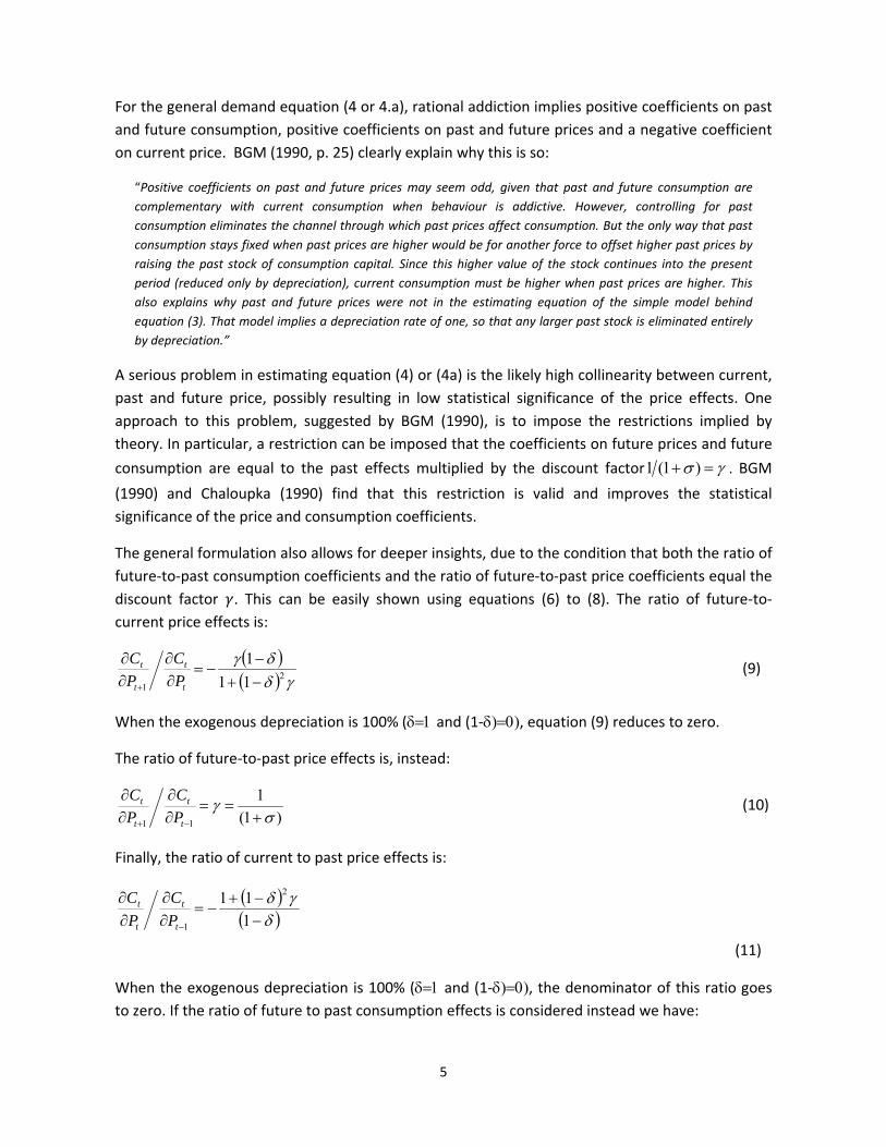
For the general demand equation (4 or 4.a), rational addiction implies positive coefficients on past
and future consumption, positive coefficients on past and future prices and a negative coefficient
on current price. BGM (1990, p. 25) clearly explain why this is so:
“Positive coefficients on past and future prices may seem odd, given that past and future consumption are
complementary with current consumption when behaviour is addictive. However, controlling for past
consumption eliminates the channel through which past prices affect consumption. But the only way that past
consumption stays fixed when past prices are higher would be for another force to offset higher past prices by
raising the past stock of consumption capital. Since this higher value of the stock continues into the present
period (reduced only by depreciation), current consumption must be higher when past prices are higher. This
also explains why past and future prices were not in the estimating equation of the simple model behind
equation (3). That model implies a depreciation rate of one, so that any larger past stock is eliminated entirely
by depreciation.”
A serious problem in estimating equation (4) or (4a) is the likely high collinearity between current,
past and future price, possibly resulting in low statistical significance of the price effects. One
approach to this problem, suggested by BGM (1990), is to impose the restrictions implied by
theory. In particular, a restriction can be imposed that the coefficients on future prices and future
consumption are equal to the past effects multiplied by the discount factor )1(1 . BGM
(1990) and Chaloupka (1990) find that this restriction is valid and improves the statistical
significance of the price and consumption coefficients.
The general formulation also allows for deeper insights, due to the condition that both the ratio of
future‐to‐past consumption coefficients and the ratio of future‐to‐past price coefficients equal the
discount factor . This can be easily shown using equations (6) to (8). The ratio of future‐to‐
current price effects is:
2
1 11
1
t
t
t
t
P
C
P
C (9)
When the exogenous depreciation is 100% (and (1‐, equation (9) reduces to zero.
The ratio of future‐to‐past price effects is, instead:
)1(
1
11
t
t
t
t
P
C
P
C (10)
Finally, the ratio of current to past price effects is:
1
11 2
1t
t
t
t
P
C
P
C
(11)
When the exogenous depreciation is 100% (and (1‐, the denominator of this ratio goes
to zero.
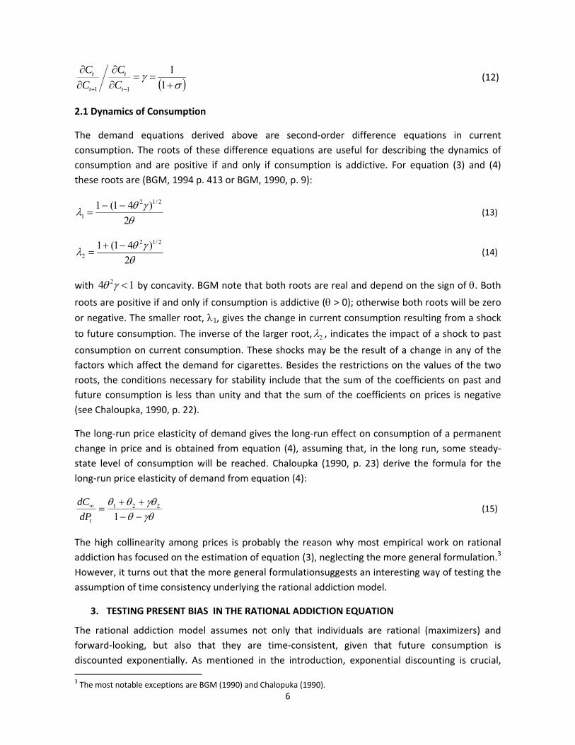
If the ratio of future to past consumption effects is considered instead we have:
6
1
1
11 t
t
t
t
C
C
C
C (12)
2.1 Dynamics of Consumption
The demand equations derived above are second‐order difference equations in current
consumption. The roots of these difference equations are useful for describing the dynamics of
consumption and are positive if and only if consumption is addictive. For equation (3) and (4)
these roots are (BGM, 1994 p. 413 or BGM, 1990, p. 9):
2
)41(1 2/12
1
(13)
2
)41(1 2/12
2
(14)
with 14 2 by concavity. BGM note that both roots are real and depend on the sign of . Both
roots are positive if and only if consumption is addictive ( > 0); otherwise both roots will be zero or negative. The smaller root, 1, gives the change in current consumption resulting from a shock
to future consumption. The inverse of the larger root, 2 , indicates the impact of a shock to past
consumption on current consumption. These shocks may be the result of a change in any of the
factors which affect the demand for cigarettes. Besides the restrictions on the values of the two
roots, the conditions necessary for stability include that the sum of the coefficients on past and
future consumption is less than unity and that the sum of the coefficients on prices is negative
(see Chaloupka, 1990, p. 22).
The long‐run price elasticity of demand gives the long‐run effect on consumption of a permanent
change in price and is obtained from equation (4), assuming that, in the long run, some steady‐
state level of consumption will be reached. Chaloupka (1990, p. 23) derive the formula for the
long‐run price elasticity of demand from equation (4):
1221
tdP
dC (15)
The high collinearity among prices is probably the reason why most empirical work on rational
addiction has focused on the estimation of equation (3), neglecting the more general formulation.3
However, it turns out that the more general formulationsuggests an interesting way of testing the
assumption of time consistency underlying the rational addiction model.
3. TESTING PRESENT BIAS IN THE RATIONAL ADDICTION EQUATION
The rational addiction model assumes not only that individuals are rational (maximizers) and
forward‐looking, but also that they are time‐consistent, given that future consumption is
discounted exponentially. As mentioned in the introduction, exponential discounting is crucial, 3 The most notable exceptions are BGM (1990) and Chalopuka (1990).

7
because it implies that utilities in any two adjacent future time periods are discounted at the same
rate or, stated differently, that individuals’ short‐run and long‐run discount rates are the same.
However, experimental evidence suggests that individuals may suffer from a present‐bias implying
a short‐run discount rate larger than the long‐run one. As a consequence of this short‐run
impatience, present‐bias generates time inconsistency. In the formulation of Laibson (1997)
present‐bias is captured by an extra discount parameter, β < 1, applied uniformly to all future
periods. As a result, consumption at time t+1 evaluated at time t will be discounted at βγ, whereas
consumption at time t+2 evaluated at time t+1, for example, will be discounted at γ. Since both β
and γ are less than one, consumption at time t+1 evaluated at t is discounted more than
consumption at any other future consecutive time period.
Starting with the work of Laibson (1997), the literature on hyperbolic discounting has grown
dramatically. Nonetheless, attempts at estimating discount functions using observational data are
still very scarce (exceptions are Laibson et al., 2007, Levy, 2010 and Paserman, 2008). The only two
empirical studies trying to find evidence against exponential discounting within the rational
addiction framework using observational data are Gruber and Köszegi (2001) and Ciccarelli et al.
(2008). Gruber and Köszegi proposed two ways of testing for time consistency, but could not
implement them due to data inadequacy. On the other hand, Ciccarelli et al. (2008) proposed a
test based on a specification that does not conform to the one derived from theory. Moreover,
their estimates conflict with theoretical predictions.
Following Laibson (1997), an individual with quasi‐hyperbolic time preferences maximizes the following utility function, where the instant gratification parameter β is between 0 and 1:
, , , ∑ , , , (16)
The discount factor between future consecutive periods is γ, but the discount factor between the
current and next period is βγ. Therefore, this type of individual prefers instant gratification over
delayed rewards.
Considering only naïve agents4, maximization of equation (16) subject to an inter‐temporal budget
constraint leads to the following second‐order difference demand equations:
1*5
*4
*11
*1
*0
* tttttt eePCCC (17)
Equation (17) is identical to equation (3) except that γβ is used instead of γ. Similarly, when δ < 1 we obtain equation (18) instead of equation (4.a):
1*1
*11
*11
*1
2*11
*1
**0 1111 tttttttt eePPPCCC (18)
Empirical estimates of equations (17) or (18) cannot identify γ and β separately. They will instead
estimate γβ. Therefore, the standard equations used to estimate rational addiction models cannot
empirically distinguish between time‐inconsistent versus time‐consistent rational addicts. These
two types of time preferences have radically different policy implications, however (Gruber and
4 See Laibson (2007) for a distinction between naïve and sophisticated quasi‐hyperbolic consumers.
8
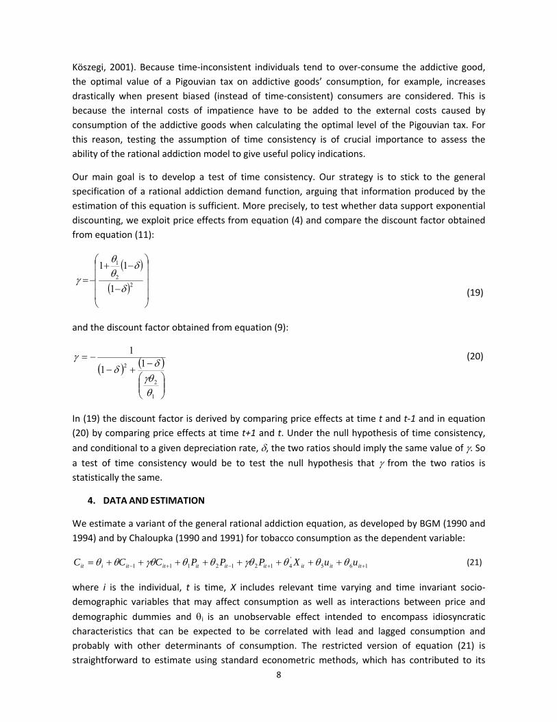
Köszegi, 2001). Because time‐inconsistent individuals tend to over‐consume the addictive good,
the optimal value of a Pigouvian tax on addictive goods’ consumption, for example, increases
drastically when present biased (instead of time‐consistent) consumers are considered. This is
because the internal costs of impatience have to be added to the external costs caused by
consumption of the addictive goods when calculating the optimal level of the Pigouvian tax. For
this reason, testing the assumption of time consistency is of crucial importance to assess the
ability of the rational addiction model to give useful policy indications.
Our main goal is to develop a test of time consistency. Our strategy is to stick to the general
specification of a rational addiction demand function, arguing that information produced by the
estimation of this equation is sufficient. More precisely, to test whether data support exponential
discounting, we exploit price effects from equation (4) and compare the discount factor obtained
from equation (11):
22
1
1
11
(19)
and the discount factor obtained from equation (9):
1
2
2 11
1
(20)
In (19) the discount factor is derived by comparing price effects at time t and t‐1 and in equation
(20) by comparing price effects at time t+1 and t. Under the null hypothesis of time consistency,
and conditional to a given depreciation rate, , the two ratios should imply the same value of . So a test of time consistency would be to test the null hypothesis that from the two ratios is
statistically the same.
4. DATA AND ESTIMATION
We estimate a variant of the general rational addiction equation, as developed by BGM (1990 and
1994) and by Chaloupka (1990 and 1991) for tobacco consumption as the dependent variable:
165'41212111 ititititititititiit uuXPPPCCC (21)
where i is the individual, t is time, X includes relevant time varying and time invariant socio‐
demographic variables that may affect consumption as well as interactions between price and
demographic dummies and i is an unobservable effect intended to encompass idiosyncratic
characteristics that can be expected to be correlated with lead and lagged consumption and
probably with other determinants of consumption. The restricted version of equation (21) is
straightforward to estimate using standard econometric methods, which has contributed to its
9
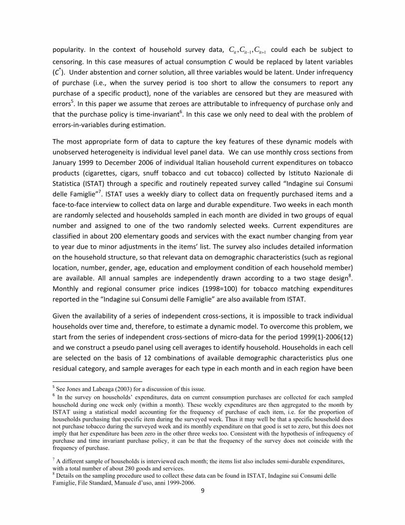
popularity. In the context of household survey data, 1 1, ,it it itC C C could each be subject to
censoring. In this case measures of actual consumption C would be replaced by latent variables
(C*). Under abstention and corner solution, all three variables would be latent. Under infrequency
of purchase (i.e., when the survey period is too short to allow the consumers to report any
purchase of a specific product), none of the variables are censored but they are measured with
errors5. In this paper we assume that zeroes are attributable to infrequency of purchase only and
that the purchase policy is time‐invariant6. In this case we only need to deal with the problem of
errors‐in‐variables during estimation.
The most appropriate form of data to capture the key features of these dynamic models with
unobserved heterogeneity is individual level panel data. We can use monthly cross sections from
January 1999 to December 2006 of individual Italian household current expenditures on tobacco
products (cigarettes, cigars, snuff tobacco and cut tobacco) collected by Istituto Nazionale di
Statistica (ISTAT) through a specific and routinely repeated survey called “Indagine sui Consumi
delle Famiglie”7. ISTAT uses a weekly diary to collect data on frequently purchased items and a
face‐to‐face interview to collect data on large and durable expenditure. Two weeks in each month
are randomly selected and households sampled in each month are divided in two groups of equal
number and assigned to one of the two randomly selected weeks. Current expenditures are
classified in about 200 elementary goods and services with the exact number changing from year
to year due to minor adjustments in the items’ list. The survey also includes detailed information
on the household structure, so that relevant data on demographic characteristics (such as regional
location, number, gender, age, education and employment condition of each household member)
are available. All annual samples are independently drawn according to a two stage design8.
Monthly and regional consumer price indices (1998=100) for tobacco matching expenditures
reported in the “Indagine sui Consumi delle Famiglie” are also available from ISTAT.
Given the availability of a series of independent cross‐sections, it is impossible to track individual
households over time and, therefore, to estimate a dynamic model. To overcome this problem, we
start from the series of independent cross‐sections of micro‐data for the period 1999(1)‐2006(12)
and we construct a pseudo panel using cell averages to identify household. Households in each cell
are selected on the basis of 12 combinations of available demographic characteristics plus one
residual category, and sample averages for each type in each month and in each region have been
5 See Jones and Labeaga (2003) for a discussion of this issue. 6 In the survey on households’ expenditures, data on current consumption purchases are collected for each sampled household during one week only (within a month). These weekly expenditures are then aggregated to the month by ISTAT using a statistical model accounting for the frequency of purchase of each item, i.e. for the proportion of households purchasing that specific item during the surveyed week. Thus it may well be that a specific household does not purchase tobacco during the surveyed week and its monthly expenditure on that good is set to zero, but this does not imply that her expenditure has been zero in the other three weeks too. Consistent with the hypothesis of infrequency of purchase and time invariant purchase policy, it can be that the frequency of the survey does not coincide with the frequency of purchase.
7 A different sample of households is interviewed each month; the items list also includes semi-durable expenditures, with a total number of about 280 goods and services. 8 Details on the sampling procedure used to collect these data can be found in ISTAT, Indagine sui Consumi delle Famiglie, File Standard, Manuale d’uso, anni 1999-2006.

10
computed. Since the survey does not provide information on the number of tobacco consumers in
the household, households with one member only have been selected to avoid any ambiguity
between the recorded expenditure and the individual in the household. Table 1 contains a
description of each average household.
Table 1 – Single household types
Household Type Male Female Young Adult Senior Low-Edu High-Edu Emp Unemp
HT1 X X X X
HT2 X X X X
HT3 X X X X HT4 X X X X HT5 X X X X
HT6 X X X X
HT7 X X X X HT8 X X X X HT9 X X
HT10 X X
HT11 X X
HT12 X X
If r is the geographical location, f is the household type, m is the month and t the year considered,
the final data have been organized as a pseudo panel Φ(r, f, m, t) by stacking up monthly data (m
=1, …, 12) for each year (t = 1, …, 8) and for each geographical region (r = 1, …, 20) on each
household type (f = 1, …,13) in vectors whose length varies each period, thus giving rise to an
unbalanced panel data set of 12,446 mean single households observations. We further collapsed
the regional data into four macro‐areas of Italy: northwest (NW); northeast (NE); central (CE);
south and the islands (SI), obtaining a final unbalanced panel of 4,259 individual observations.
Our dependent variable, the quantity of tobacco consumed, has been obtained implicitly as the
ratio between monthly tobacco expenditure (in Euros) and the tobacco price index. In order to
introduce some individual variation, the price of tobacco is constructed by deflating the retail price
index for tobacco by a weighted average of nine broad categories of the retail price index, as in
Labeaga (1999), where the weights are the shares of expenditure devoted to each good in each
household. A set of dummy variables is included to account for socio‐demographic and geographic
factors: location ; gender; employment status (employed, unemployed); education level (higher
education, lower education); income level (rich, poor, middle); age (less than 24 years; between
25 and 65 years and more than 65 years); household type (1 to 13) based on gender, age,
employment condition and education level of the single member of the household according to
combinations displayed in table 1. We also add total current monthly expenditure as a proxy of
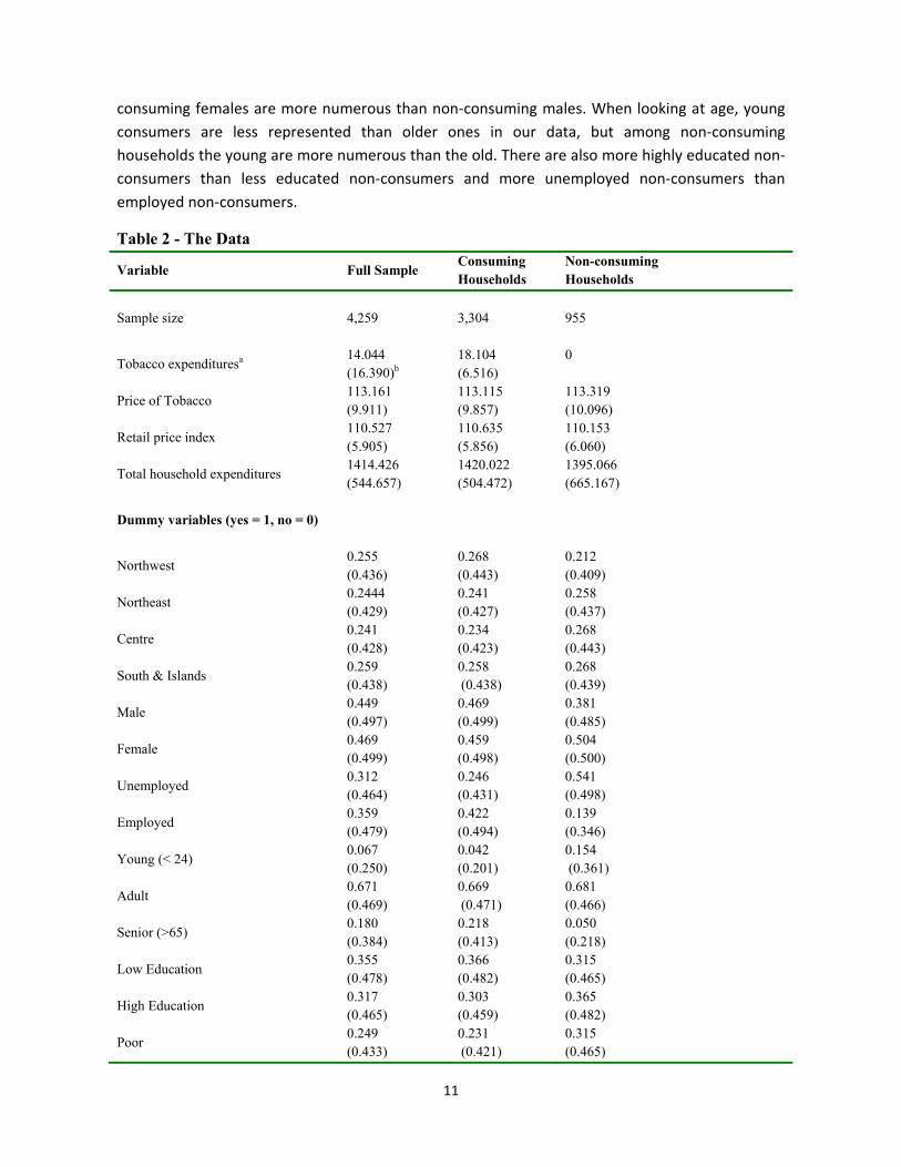
disposable income. Summary statistics of the data are shown in table 2. Almost 22% of the single
households report zero tobacco expenditures during the survey period. On average, tobacco
consuming singles have slightly higher total expenditures than non‐consuming ones. Non‐
11
consuming females are more numerous than non‐consuming males. When looking at age, young
consumers are less represented than older ones in our data, but among non‐consuming
households the young are more numerous than the old. There are also more highly educated non‐
consumers than less educated non‐consumers and more unemployed non‐consumers than
employed non‐consumers.
Table 2 - The Data
Variable Full Sample Consuming Households
Non-consuming Households
Sample size
4,259
3,304
955
Tobacco expendituresa 14.044 (16.390)b
18.104 (6.516)
0
Price of Tobacco 113.161 (9.911)
113.115 (9.857)
113.319 (10.096)
Retail price index 110.527 (5.905)
110.635 (5.856)
110.153 (6.060)
Total household expenditures 1414.426 (544.657)
1420.022 (504.472)
1395.066 (665.167)
Dummy variables (yes = 1, no = 0)
Northwest 0.255 (0.436)
0.268 (0.443)
0.212 (0.409)
Northeast 0.2444 (0.429)
0.241 (0.427)
0.258 (0.437)
Centre 0.241 (0.428)
0.234 (0.423)
0.268 (0.443)
South & Islands 0.259 (0.438)
0.258 (0.438)
0.268 (0.439)
Male 0.449 (0.497)
0.469 (0.499)
0.381 (0.485)
Female 0.469 (0.499)
0.459 (0.498)
0.504 (0.500)
Unemployed 0.312 (0.464)
0.246 (0.431)
0.541 (0.498)
Employed 0.359 (0.479)
0.422 (0.494)
0.139 (0.346)
Young (< 24) 0.067 (0.250)
0.042 (0.201)
0.154 (0.361)
Adult 0.671 (0.469)
0.669 (0.471)
0.681 (0.466)
Senior (>65) 0.180 (0.384)
0.218 (0.413)
0.050 (0.218)
Low Education 0.355 (0.478)
0.366 (0.482)
0.315 (0.465)
High Education 0.317 (0.465)
0.303 (0.459)
0.365 (0.482)
Poor 0.249 (0.433)
0.231 (0.421)
0.315 (0.465)
12
Rich 0.249 (0.433)
0.249 (0.432)
0.252 (0.435)
Middle 0.500 (0.500)
0.519 (0.499)
0.432 (0.496)
Notes: 1. Monthly expenditures in Euros 2. Standard deviations in parentheses. Source: ISTAT, “I Consumi delle Famiglie”, years 1999-2006.
4.1 Estimation Method
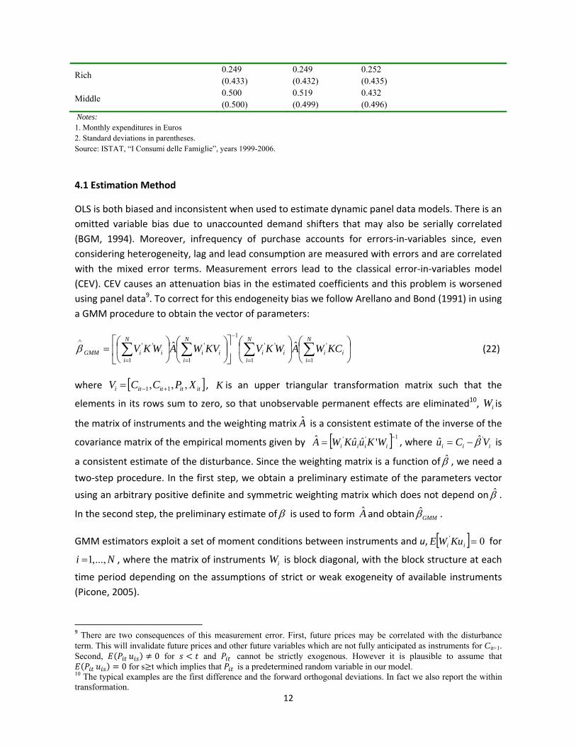
OLS is both biased and inconsistent when used to estimate dynamic panel data models. There is an
omitted variable bias due to unaccounted demand shifters that may also be serially correlated
(BGM, 1994). Moreover, infrequency of purchase accounts for errors‐in‐variables since, even
considering heterogeneity, lag and lead consumption are measured with errors and are correlated
with the mixed error terms. Measurement errors lead to the classical error‐in‐variables model
(CEV). CEV causes an attenuation bias in the estimated coefficients and this problem is worsened
using panel data9. To correct for this endogeneity bias we follow Arellano and Bond (1991) in using
a GMM procedure to obtain the vector of parameters:
N
iii
N
iii
N
iii
N
iiiGMM KCWAWKVKVWAWKV
1
'
1
''
1
1
'
1
'' ˆˆ (22)
where ititititi XPCCV ,,, 11 , K is an upper triangular transformation matrix such that the
elements in its rows sum to zero, so that unobservable permanent effects are eliminated10, iW is
the matrix of instruments and the weighting matrix A is a consistent estimate of the inverse of the
covariance matrix of the empirical moments given by 1'' 'ˆˆˆ iiii WKuuKWA , where iii VCu 'ˆˆ is
a consistent estimate of the disturbance. Since the weighting matrix is a function of , we need a
two‐step procedure. In the first step, we obtain a preliminary estimate of the parameters vector
using an arbitrary positive definite and symmetric weighting matrix which does not depend on .
In the second step, the preliminary estimate of is used to form A and obtain GMM .
GMM estimators exploit a set of moment conditions between instruments and u, 0' ii KuWE for
Ni ...,,1 , where the matrix of instruments iW is block diagonal, with the block structure at each
time period depending on the assumptions of strict or weak exogeneity of available instruments
(Picone, 2005).
9 There are two consequences of this measurement error. First, future prices may be correlated with the disturbance term. This will invalidate future prices and other future variables which are not fully anticipated as instruments for Cit+1. Second, 0 for and cannot be strictly exogenous. However it is plausible to assume that
0 for s t which implies that is a predetermined random variable in our model. 10 The typical examples are the first difference and the forward orthogonal deviations. In fact we also report the within transformation.
13
An augmented version of the above estimator with better finite sample properties can be
obtained incorporating extra orthogonality conditions for the equations in levels. This is the
system‐GMM (Blundell and Bond, 1998), which allows for orthogonality conditions of both
transformed IK and in level IK equations.
Whether we actually need all these moment conditions is debatable, since in finite samples there
is a bias/efficiency trade‐off. For example, Ziliak (1997) showed that GMM may perform better
with suboptimal instruments and argued against using all available moments, especially when T is
large relative to N. Since in our case N = 52 and T = 96 (hence a large number of orthogonality
conditions), we use only a subset of them, testing their validity with the Sargan over‐identification
test (Baltagi and Griffin, 2001).
Finally, we have to choose a set of instruments. Ever since the work of BGM (1994) on US cigarette
consumption, past and future prices have been considered natural instruments for lagged and
lead consumption. In fact, their empirical support of the rational addiction theory relies heavily on
future prices. Exclusion of them from the instrument set yields puzzling results, such as negative
interest rates and wrong sings on lagged consumption and own price. So, despite future prices
failing a Hausman test, BGM (1994) consider them as valid instruments on several grounds.
Specifically, they argue that smokers may have sufficient information on taxation policy to
anticipate any cigarette price upswing in advance. Whether their conjecture is legitimate in
general or depends on data makes a difference in terms of the stacked matrix iW . For example, it
is unlikely that Italian consumers may have relevant information to forecast tobacco price
changes. This invalidates future prices as well as other variables which are not fully anticipated at
time t as instruments for future consumption of tobacco. At the same time, over our study period
the real price series does not show so much time variation that individuals can possibly forecast
tobacco prices a month or more from the date of the survey, thus partly reviving BGM’s (1994)
conjecture.
The use of prices alone to instrument consumption can induce problems of weak instruments and
problems of estimators that can be biased towards ordinary least squares (see Jones and Labeaga,
2003, for a discussion of this issue). Time invariant demographic variables can also be used as
instruments in any transformation of the model that rules out time invariant explanatory
variables. After some experimentation with the matrix of instruments iW , we use lag and lead
prices, the proxy of disposable income as well as a number of demographic variables. One way to
decide about the set of instruments is to perform a Hausman test of the null hypothesis that
future prices are legitimate instruments.11
5. RESULTS
The empirical specification of model (21) uses the quantity of tobacco consumed per month as the
dependent variable. The right‐hand side variables are the lead and lag consumption, the current
11 Estimation of the model employs a modified TSP program written by Yoshitsugu Kitazawa (2003). The set of TSP scripts can be obtained from http://www.ip.kyusan-u.ac.jp/J/kitazawa/SOFT/TSP_DPD1/index.htm.
14
lead and lag real price of tobacco, the proxy of disposable income and the following socio‐
demographic characteristics: gender, age, high education, high income and the interactions
between price and demographic characteristics. We use a subset of all available instruments of
prices. Our chosen estimator is the system–GMM (Blundell and Bond, 1998). This unifying GMM
framework incorporates orthogonality conditions of both types of equations, transformed and in
levels and performs significantly better in terms of efficiency as compared to other IV estimators
of dynamic panel data models. We estimate both one‐step and two‐step system‐GMM estimators,
but we only report two‐step estimates with a robust covariance matrix12.
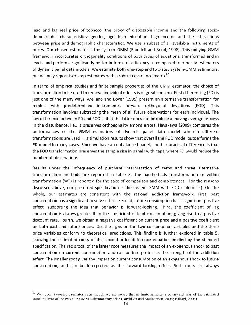
In terms of empirical studies and finite sample properties of the GMM estimator, the choice of
transformation to be used to remove individual effects is of great concern. First differencing (FD) is
just one of the many ways. Arellano and Bover (1995) present an alternative transformation for
models with predetermined instruments, forward orthogonal deviations (FOD). This
transformation involves subtracting the mean of all future observations for each individual. The
key difference between FD and FOD is that the latter does not introduce a moving average process
in the disturbance, i.e., it preserves orthogonality among errors. Hayakawa (2009) compares the
performances of the GMM estimators of dynamic panel data model wherein different
transformations are used. His simulation results show that overall the FOD model outperforms the
FD model in many cases. Since we have an unbalanced panel, another practical difference is that
the FOD transformation preserves the sample size in panels with gaps, where FD would reduce the
number of observations.
Results under the infrequency of purchase interpretation of zeros and three alternative
transformation methods are reported in table 3. The fixed‐effects transformation or within
transformation (WT) is reported for the sake of comparison and completeness. For the reasons
discussed above, our preferred specification is the system GMM with FOD (column 2). On the
whole, our estimates are consistent with the rational addiction framework. First, past
consumption has a significant positive effect. Second, future consumption has a significant positive
effect, supporting the idea that behavior is forward‐looking. Third, the coefficient of lag
consumption is always greater than the coefficient of lead consumption, giving rise to a positive
discount rate. Fourth, we obtain a negative coefficient on current price and a positive coefficient
on both past and future prices. So, the signs on the two consumption variables and the three
price variables conform to theoretical predictions. This finding is further explored in table 5,
showing the estimated roots of the second‐order difference equation implied by the standard
specification. The reciprocal of the larger root measures the impact of an exogenous shock to past
consumption on current consumption and can be interpreted as the strength of the addiction
effect. The smaller root gives the impact on current consumption of an exogenous shock to future
consumption, and can be interpreted as the forward‐looking effect. Both roots are always
12 We report two-step estimates even though we are aware that in finite samples a downward bias of the estimated standard error of the two-step GMM estimator may arise (Davidson and MacKinnon, 2004; Baltagi, 2005).

15
significantly positive. Our results fulfill the stability condition13 as both roots are positive and
4 1(BGM, 1994). Finally, the sum of coefficients on past and future consumption is less
than unity and the sum of price coefficients is negative, as required by theory.
Table 3 – Estimation of General Rational Addiction Models (infrequency or misreporting) Parameter Gmm_Sys Gmm_Sys Gmm_Sys
WT FOD FD
Ct-1 0.506 (0.007)
0.483 (0.009)
0.055 (0.021)
Ct+1 0.486 (0.006)
0.461 (0.008)
0.045 (0.020)
Pt -0.474 (0.090)
-0.385 (0.093)
-0.515 (0.092)
Pt-1 0.243 (0.042)
0.225 (0.055)
0.314 (0.052)
Pt+1 0.229 (0.050)
0.150 (0.057)
0.194 (0.078)
Northwest 1.926 (5.020)
-3.837 (3.311)
Northeast 15.290 (4.979)
-14.043 (3.390)
Centre 3.373 (4.945)
-11.337 (3.126)
Male -6.457 (7.303)
0.952 (4.261)
6.494 (1.266)
Employed -9.418 (10.427)
-2.483 (6.435)
1.801 (2.295)
Adult -14.524 (6.427)
11.834 (4.006)
2.790 (1.858)
College 12.253 (12.746)
1.081 (6.507)
-4.993 (1.872)
Rich 3.349 (0.589)
2.587 (1.160)
Price*Male 0.014 (0.018)
0.041 (0.010)
Price*Employed -0.010 (0.022)
-0.038 (0.013)
Price*Adult -0.019 (0.023)
-0.014 (0.011)
Price*College 0.008 (0.068)
0.028 (0.010)
Male*Employed 9.987 (20.374)
5.046 (11.400)
Male*Adult 0.677 (18.451)
-8.497 (10.227)
Male*College 4.688 (16.956)
-5.644 (9.516)
p-value Sargan test 0.427 0.519 0.322
1. Instrument set: lagged and lead prices, expenditure and demographic dummies for lagged and lead consumption. 2. Consistent standard errors robust to heteroscedasticity are in parentheses.
The proxy of disposable income has a small and positive effect on current consumption of tobacco. As to the demographic variables in our specification, being an adult has a positive and significant
13 Baltagi (2007) stresses that, in fact, this is somehow improperly known as a stability condition, because the solution to a rational addiction model is generally assumed to be a saddle point and its roots could therefore not pass a stability test.
16
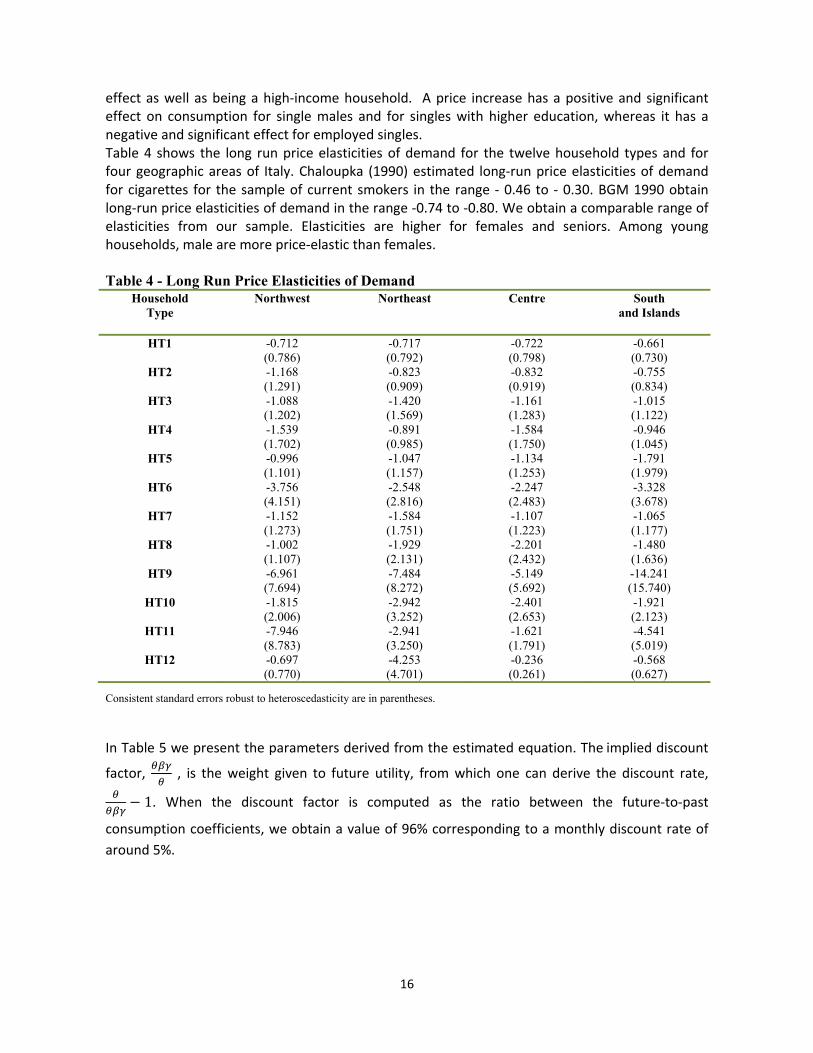
effect as well as being a high‐income household. A price increase has a positive and significant effect on consumption for single males and for singles with higher education, whereas it has a negative and significant effect for employed singles. Table 4 shows the long run price elasticities of demand for the twelve household types and for four geographic areas of Italy. Chaloupka (1990) estimated long‐run price elasticities of demand for cigarettes for the sample of current smokers in the range ‐ 0.46 to ‐ 0.30. BGM 1990 obtain long‐run price elasticities of demand in the range ‐0.74 to ‐0.80. We obtain a comparable range of elasticities from our sample. Elasticities are higher for females and seniors. Among young households, male are more price‐elastic than females. Table 4 - Long Run Price Elasticities of Demand
Household Type
Northwest Northeast Centre South and Islands
HT1 -0.712
(0.786) -0.717 (0.792)
-0.722 (0.798)
-0.661 (0.730)
HT2 -1.168 (1.291)
-0.823 (0.909)
-0.832 (0.919)
-0.755 (0.834)
HT3 -1.088 (1.202)
-1.420 (1.569)
-1.161 (1.283)
-1.015 (1.122)
HT4 -1.539 (1.702)
-0.891 (0.985)
-1.584 (1.750)
-0.946 (1.045)
HT5 -0.996 (1.101)
-1.047 (1.157)
-1.134 (1.253)
-1.791 (1.979)
HT6 -3.756 (4.151)
-2.548 (2.816)
-2.247 (2.483)
-3.328 (3.678)
HT7 -1.152 (1.273)
-1.584 (1.751)
-1.107 (1.223)
-1.065 (1.177)
HT8 -1.002 (1.107)
-1.929 (2.131)
-2.201 (2.432)
-1.480 (1.636)
HT9 -6.961 (7.694)
-7.484 (8.272)
-5.149 (5.692)
-14.241 (15.740)
HT10 -1.815 (2.006)
-2.942 (3.252)
-2.401 (2.653)
-1.921 (2.123)
HT11 -7.946 (8.783)
-2.941 (3.250)
-1.621 (1.791)
-4.541 (5.019)
HT12 -0.697 (0.770)
-4.253 (4.701)
-0.236 (0.261)
-0.568 (0.627)
Consistent standard errors robust to heteroscedasticity are in parentheses.
In Table 5 we present the parameters derived from the estimated equation. Theimplied discount
factor, , is the weight given to future utility, from which one can derive the discount rate,
1. When the discount factor is computed as the ratio between the future‐to‐past
consumption coefficients, we obtain a value of 96% corresponding to a monthly discount rate of
around 5%.
17
Table 5 – Strength of Addiction, Discount Rate and Time Consistency
Derived parameter Model 1 Model 2 Model 3 Model 4
δ=0.20 δ=0.25 δ=0.30 δ=0.35
(Larger root)-1 3.115
(0.052)
Smaller root 0.162
(0.000)
Monthly discount factor
0.966 (0.029)
Monthly discount rate 0.047
(0.031)
[βγ]1
0.689 (0.253)
0.711 (0.254)
0.769 (0.260)
0.806 (0.265)
[βγ] 2
0.624 (0.270)
0.571 (0.287)
0.398 (0.328)
0.259 (0.353)
[βγ]1 - [βγ]2
0.065 (0.059)
0.140 (0.066)
0.371 (0.092)
0.547 (0.110)
β 0.905
(0.097) 0.803
(0.137) 0.517
(0.258) 0.321
(0.335)
γ 0.689
(0.253) 0.711
(0.254) 0.769
(0.260) 0.806
(0.265)
Consistent standard errors robust to heteroscedasticity are in parentheses.
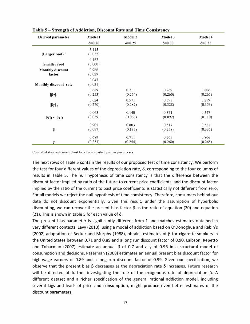
The next rows of Table 5 contain the results of our proposed test of time consistency. We perform
the test for four different values of the depreciation rate, δ, corresponding to the four columns of
results in Table 5. The null hypothesis of time consistency is that the difference between the
discount factor implied by ratio of the future to current price coefficients and the discount factor
implied by the ratio of the current to past price coefficients is statistically not different from zero.
For all models we reject the null hypothesis of time consistency. Therefore, consumers behind our
data do not discount exponentially. Given this result, under the assumption of hyperbolic
discounting, we can recover the present‐bias factor β as the ratio of equation (20) and equation
(21). This is shown in table 5 for each value of δ.
The present bias parameter is significantly different from 1 and matches estimates obtained in
very different contexts. Levy (2010), using a model of addiction based on O’Donoghue and Rabin’s
(2002) adaptation of Becker and Murphy (1988), obtains estimates of β for cigarette smokers in
the United States between 0.71 and 0.89 and a long run discount factor of 0.90. Laibson, Repetto
and Tobacman (2007) estimate an annual β of 0.7 and a γ of 0.96 in a structural model of
consumption and decisions. Paserman (2008) estimates an annual present bias discount factor for
high‐wage earners of 0.89 and a long run discount factor of 0.99. Given our specification, we
observe that the present bias β decreases as the depreciation rate δ increases. Future research
will be directed at further investigating the role of the exogenous rate of depreciation δ. A
different dataset and a richer specification of the general rational addiction model, including
several lags and leads of price and consumption, might produce even better estimates of the
discount parameters.
18
6. CONCLUDING REMARKS
This paper addresses one of the main theoretical and empirical shortcomings of the rational
addiction model, namely that forward‐looking behavior, implied by theory, does not necessarily
imply time consistency. So, even when forward‐looking behavior can be convincingly supported,
the dynamic consumption equation derived from the rational addiction theory does not provide
evidence in favor of time‐consistent preferences against a model with dynamic inconsistency
(Gruber and Köszegi, 2001).
In fact we show that the possibility of testing for time consistency and of separately identifying a
present bias and a long‐run discount parameter is nested within the rational addiction demand
equation. Rather than relying on additional assumptions or on a different theoretical and/or
empirical framework, we use price effects and the rarely estimated general formulation of the
rational addiction demand equation to develop a test of time consistency. The test’s purpose is to
check whether consumers behind our data reveal time‐consistent preferences or not.
Our results for the general rational addiction model conform to theory. We also find evidence of
time inconsistency in all of our specifications. Conditional on this evidence, under the assumption
of quasi‐hyperbolic discounting, we propose a simple way of recovering the short and long run
discount parameters separately. Our derived estimates of the short and long run discount
parameters are plausible, statistically significant and in line with the literature.
Our conclusion is that the possibility of distinguishing time‐consistent from time‐inconsistent
preferences is nested within the rational addiction model. The information extracted from a
general rational addiction demand equation is sufficient to test for both forward‐looking behavior
and time consistency. Future efforts will be directed at further investigating the role of the
exogenous rate of depreciation δ.
References
Acland, D. and M. Levy (2010) “Habit Formation, Naiveté, and Projection Bias in Gym Attendance.”
Working Paper, Harvard University.
Ainslie, G. (1992) “Picoeconomics: the Strategic Interaction of Successive Motivational States
Within the Person.” Cambridge, UK; New York: Cambridge University Press, 1992.
Angeletos, G., D. Laibson, A. Repetto, J. Tobacman and S. Weinberg (2001) “The Hyperbolic
Consumption Model: Calibration, Simulation and Empirical Evaluation.” The Journal of Economic
Perspectives, Summer 2001, 15(3), pp. 47‐68.
Arellano, M. and O. Bover (1995) “Another look at the Instrumental Variable Estimation of error‐
component Models.” Journal of Econometrics, 68, pp. 29‐51.
19
Arellano, M. and S. Bond (1991) “Some tests of specification for panel data: Monte Carlo evidence
and an application to employment equations.” Review of Economic Studies, 58, pp. 277‐297.
Baltagi, B. (2005) Econometric Analysis of Panel Data. John Wiley & Sons.
Baltagi, B. (2007) “On the use of Panel Data to estimate Rational Addiction Models.” Scottish Journal of Political Economy, 54(1), pp. 1–18.
Baltagi, B. and Griffin, J.M. (2001) “The Econometrics of Rational Addiction: the Case of
Cigarettes.” Journal of Business and Economic Statistics, 11: 4, pp. 449‐454.
Barro, R. J. (1999) “Ramsey meets Laibson in the neoclassical growth model.” Quarterly Journal of
Economics, 114, pp. 1125‐1152.
Becker, G. S. and K. Murphy (1988) “A Theory of Rational Addiction.” Journal of Political Economy,
96, pp. 675‐701.
Becker, G., M. Grossman and K. Murphy (1990) “An Empirical Analysis of Cigarette Addiction.”
Working Paper n. 61‐1990. Centre for the Study of the Economy and the State, University of
Chicago.
Becker, G. S., M. Grossman, K.M. Murphy (1994) “An Empirical Analysis of Cigarette Addiction.”
The American Economic Review, pp. 396‐418.
Blundell, R. and S. Bond (1998) “Initial conditions and moment restrictions in dynamic panel data
models.” Journal of Econometrics, 87, pp. 115‐143.
Chaloupka, F. (1990) “Rational Addictive Behaviour and Cigarette Smoking.” NBER Working Paper
n. 3268/1990.
Chaloupka, F. (1991) “Rational Addictive Behavior and Cigarette Smoking.” Journal of Political
Economy, 99, 4, pp. 722‐742.
Ciccarelli, C., L. Giamboni and R. Waldmann (2008) “Cigarette Smoking, Pregnancy, Forward‐
looking Behavior and Dynamic Inconsistency”. Munich Personal RePEc Archive No. 8878.
Davidson, R. and J.G. Mackinnon (2004) Econometric Theory and Methods. Oxford University
Press, 2004.
Della Vigna, S. (2009) “Psychology and Economics: Evidence from the Field.” Journal of Economic
Literature, August 2009, 47(2), pp. 315‐372.
Della Vigna, S. and D. Paserman (2005) “Job Search and Impatience.” Journal of Labor Economics,
23(3), pp. 527‐588.
Diamond, P. and B. Köszegi (1998) “Hyperbolic Discounting and Retirement.” Mimeo, 1998.
20
Fang, H. and D. Silverman (2009) “Time inconsistency and Welfare Program Participation.
Evidence from the NLSY.” International Economic Review, vol. 50, n. 4, pp. 1043‐1076.
Gruber, J. and B. Köszegi (2000) “Is Addiction Rational? Theory and Evidence.” NBER Working
Paper 7507.
Gruber, J. and B. Köszegi (2001) “Is Addiction Rational? Theory and Evidence.” Quarterly Journal of
Economics, CXVI, pp. 1261-1303.
Hayakawa K. (2009) “First Difference or Forward Orthogonal Deviation – Which Transformation
Should Be Used in Dynamic Panel Data?: A Simulation Study.” Economics Bulletin, Vol. 29,no. 3,
pp. 2008‐2017.
Jones, A. and J.M. Labeaga (2003) “Individual Heterogeneity and Censoring in Panel data Estimates
of Tobacco Expenditure.” Journal of Applied Econometrics, 18, pp. 157‐177.
Labeaga, J. M. (1999) “A Double‐Hurdle rational addiction model with heterogeneity: estimating
the demand for tobacco.” Journal of Econometrics, 93:1, pp. 49‐72.
Laibson, D. (1997) “Golden Eggs and Hyperbolic Discounting”. Quarterly Journal of Economics,
62:2, pp. 443‐478.
Laibson, D., A. Repetto and J. Tobacman (2007) “Estimating Discount Functions with Consumption
Choices Over the Lifecycle.” Working Paper, Harvard University.
Levy, M. (2010) “An Empirical Analysis of Biases in Cigarette Addiction.” Working Paper, Harvard
University.
Loewenstein, G. and J. Elster (1992) “Choice over Time.” Russell Sage: New York, 1992.
O’Donoghue, T. and M. Rabin (1999a) “Doing it Now or Later.” The American Economic Review,
89(1), pp. 103‐124.
O’Donoghue, T. and M. Rabin (1999b) “Addiction and Self‐Control.” In Jon Elster, editor, Addiction:
Entries and Exits, New York: Russell Sage.
O’Donoghue, T. and M. Rabin (2002) “Addiction and Present Biased Preferences.” University of
California at Berkeley, Working paper 1039.
Paserman, D. (2008) “Job Search and Hyperbolic Discounting: Structural Estimation and Policy
Evaluation.” Economic Journal, 118(531), pp. 1418‐1452.
Picone, G. (2005) “GMM Estimators, Instruments and the Economics of Addiction.” Unpublished
manuscript.
Shapiro, J. (2005) “Is There a Daily Discount Rate? Evidence from the Food Stamp Nutrition Cycle.”
Journal of Public Economics, 2005, 89(2), pp. 303‐325.

21
Strotz, R.H. (1956) “Myopia and Inconsistency in Dynamic Utility Maximization.” The Review of
Economic Studies, 23(3), pp. 165‐180.
Ziliak, J.P. (1997) “Efficient estimation with panel data when instruments are predetermined: an empirical comparison of moment‐condition estimators.” Journal of Business and Economics Statistics, 15, pp. 419‐431.