Vector Field Analysis

Other Features

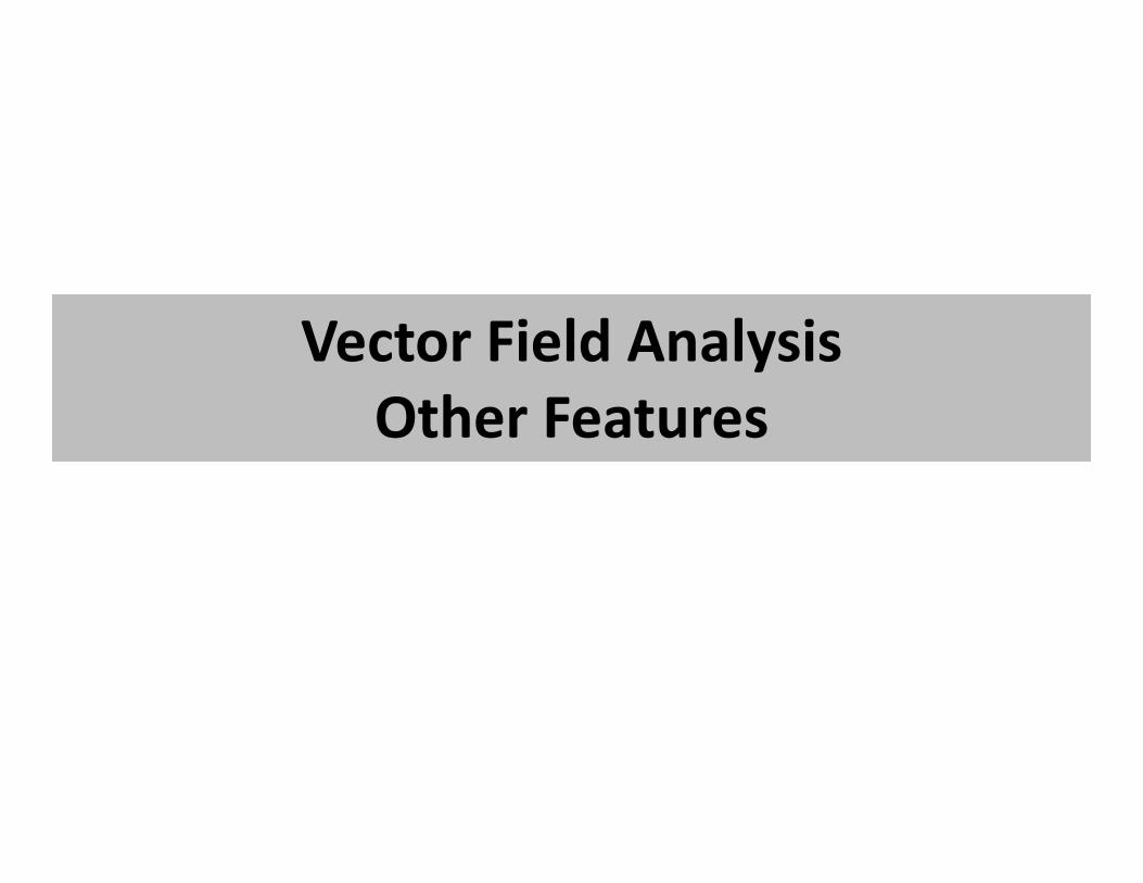
Topological Features

• Flow recurrence and their

connectivity

• Separation structure that

classifies the particle

advection

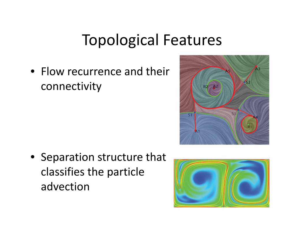
Vector Field Gradient Recall

• Consider a vector field

�� ��� = � � = � �, , � =� ����

• Its gradient is

�� =

�� ��

�� �

�� ��

�����

����

�����

�����

����

�����

It is also called the Jacobian matrix of the vector field.

Many feature detection for flow data relies on Jacobian

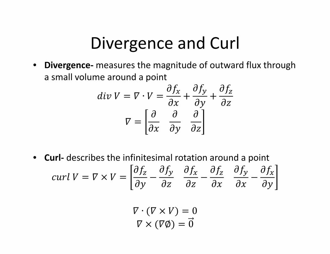
Divergence and Curl• Divergence- measures the magnitude of outward flux through

a small volume around a point

���� = � ∙ � = �� �� + ���

� + �����

� = ���

��

���

• Curl- describes the infinitesimal rotation around a point

����� = � × � = ���� −

�����

�� �� −

�����

����� − ��

�

� ∙ (� × �) = 0� × (�∅) = 0

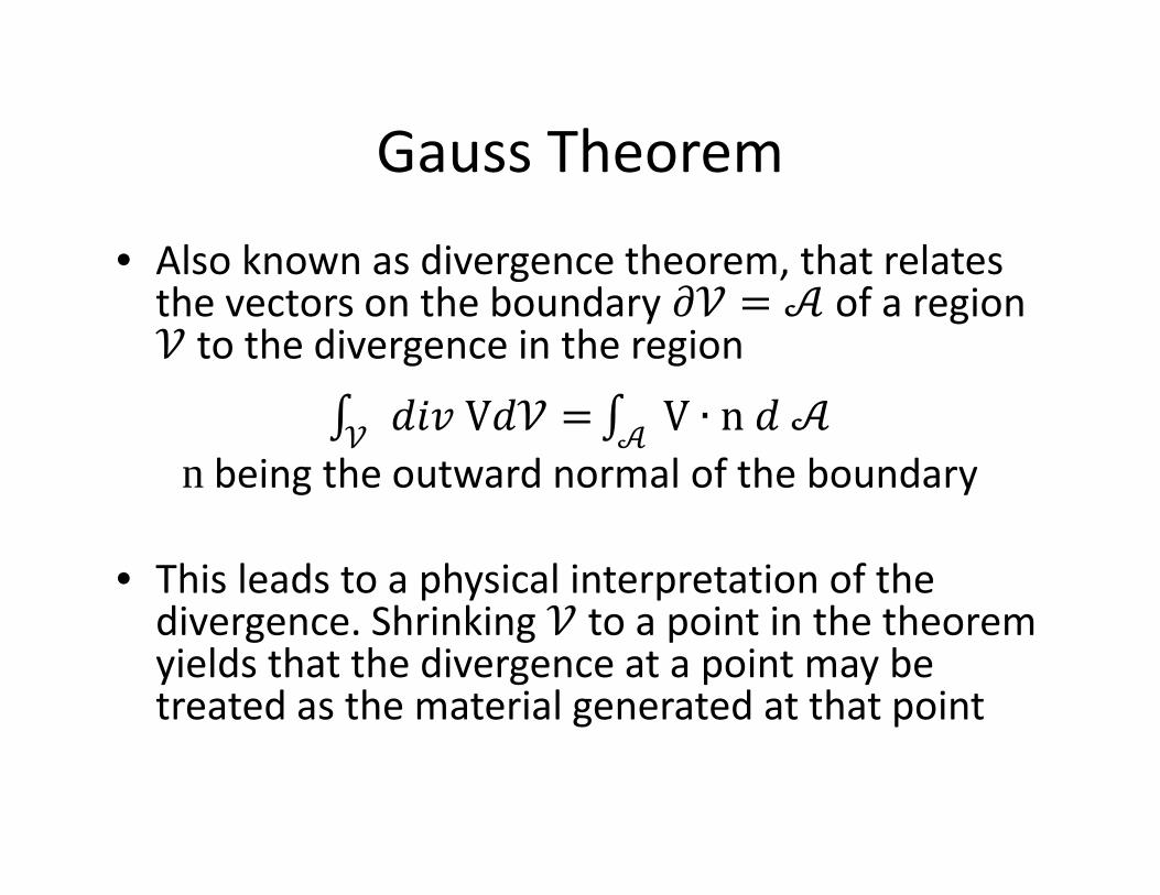
Gauss Theorem

• Also known as divergence theorem, that relates the vectors on the boundary �! = "of a region ! to the divergence in the region

# ���V�! =! # V ∙ n�" "n being the outward normal of the boundary

• This leads to a physical interpretation of the divergence. Shrinking ! to a point in the theorem yields that the divergence at a point may be treated as the material generated at that point

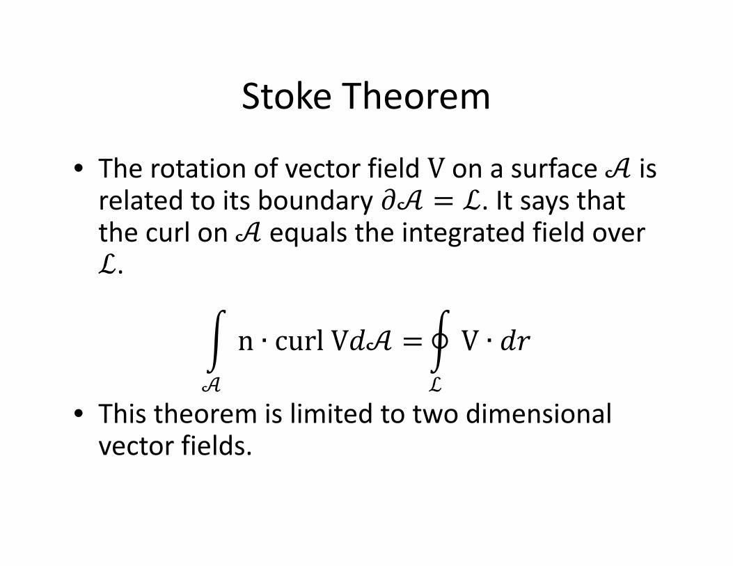
Stoke Theorem

• The rotation of vector field V on a surface "is related to its boundary �" = ℒ. It says that the curl on "equals the integrated field over ℒ.

' n ∙ curlV�" ="

, V ∙ ��ℒ

• This theorem is limited to two dimensional vector fields.

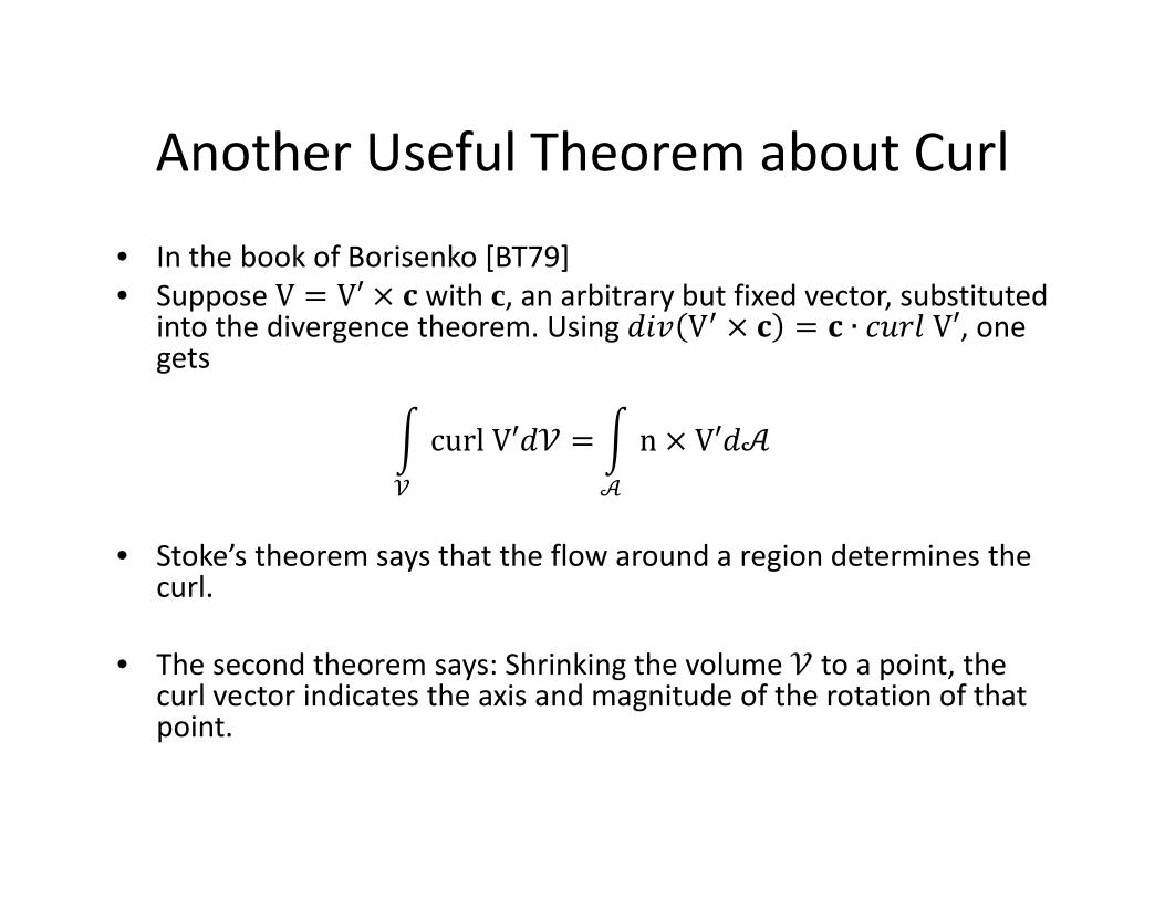
Another Useful Theorem about Curl

• In the book of Borisenko [BT79]

• Suppose V = V′ × . with c, an arbitrary but fixed vector, substituted into the divergence theorem. Using ��� V/ × . = . ∙ ����V′, one gets

' curlV′�! =!

' n × V′�""

• Stoke’s theorem says that the flow around a region determines the curl.

• The second theorem says: Shrinking the volume ! to a point, the curl vector indicates the axis and magnitude of the rotation of that point.

2D Vector Field Recall

• Assume a 2D vector field

�� ��� = � � = � �, = � �� = 0� + 1 + ��� + 2 + �

• Its Jacobian is

�� =�� ��

�� �

�����

����

= 0 1� 2

• Divergence is 0 + 2• Curl is b − dGiven a vector field defined on a discrete mesh, it is important

to compute the coefficients a, b, c, d, e, f for later analysis.

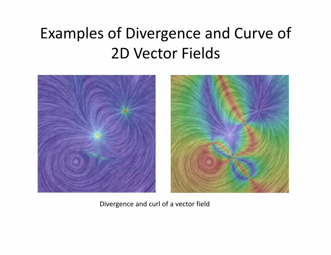
Examples of Divergence and Curve of

2D Vector Fields

Divergence and curl of a vector field

Potential or Irrotational Fields

• A vector field V is said to be a potential field if there exists a scalar field 5with

V = grad5 = �55 is called the scalar potential of the vector field V

• A vector field V living on a simply connected region is irrotational, i.e. curlV = 0 (i.e. curl-free), if and only if it is a potential field.

• It is worth noting that the potential defining the potential field is not unique, because

grad 8 + � = grad8 + grad� = grad8 + 0 = grad8

Solenoidal Fields

• Or divergence-free field

V = curlΦ = � × Φ• Solenoidal fields stem from potentials too, but this time from

vector potentials, Φ.

• These fields can describe incompressible fluid flow and are therefore as important as potential fields.

• A vector field V is solenoidal, i.e. � = � × Φ with Φ ∶ ℝ< → ℝ>, if and only if the divergence of V vanishes.

• The vector potential here is not unique as well

curl V + �8 = curlV + curl�8 = curlV + 0 = curlV

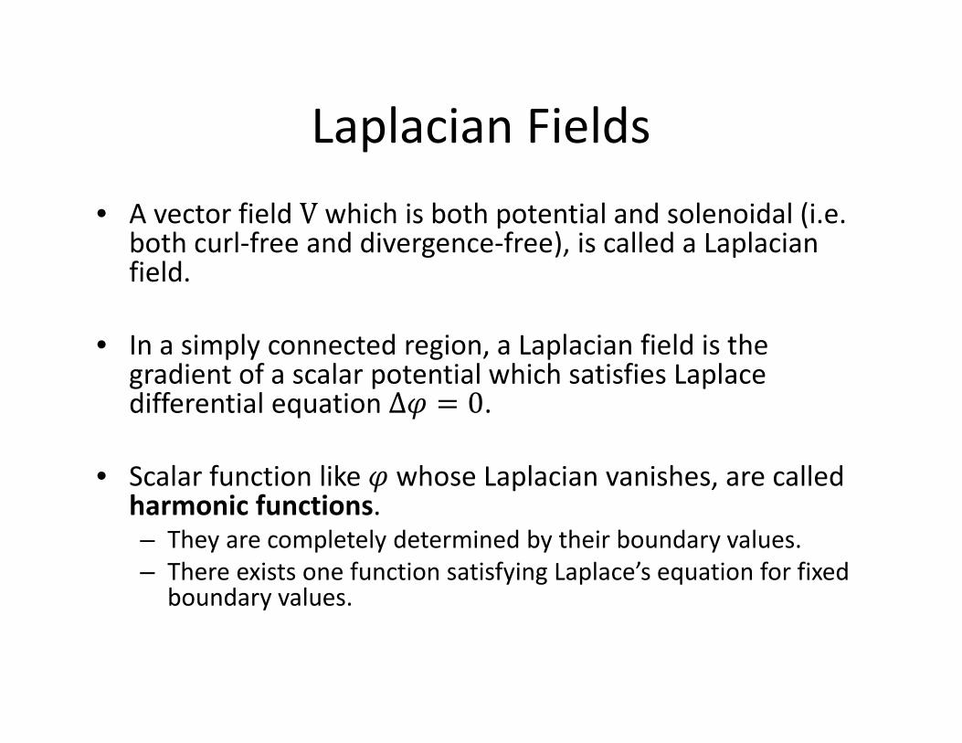
Laplacian Fields

• A vector field V which is both potential and solenoidal (i.e. both curl-free and divergence-free), is called a Laplacianfield.

• In a simply connected region, a Laplacian field is the gradient of a scalar potential which satisfies Laplace differential equation ∆5 = 0.

• Scalar function like 5 whose Laplacian vanishes, are called harmonic functions.– They are completely determined by their boundary values.

– There exists one function satisfying Laplace’s equation for fixed boundary values.

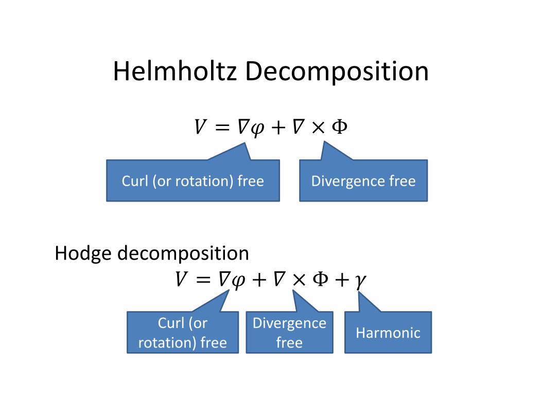
Helmholtz Decomposition

� = �5 + � × Φ

Hodge decomposition

� = �5 + � × Φ+ @

Curl (or rotation) free Divergence free

Curl (or

rotation) free

Divergence

freeHarmonic

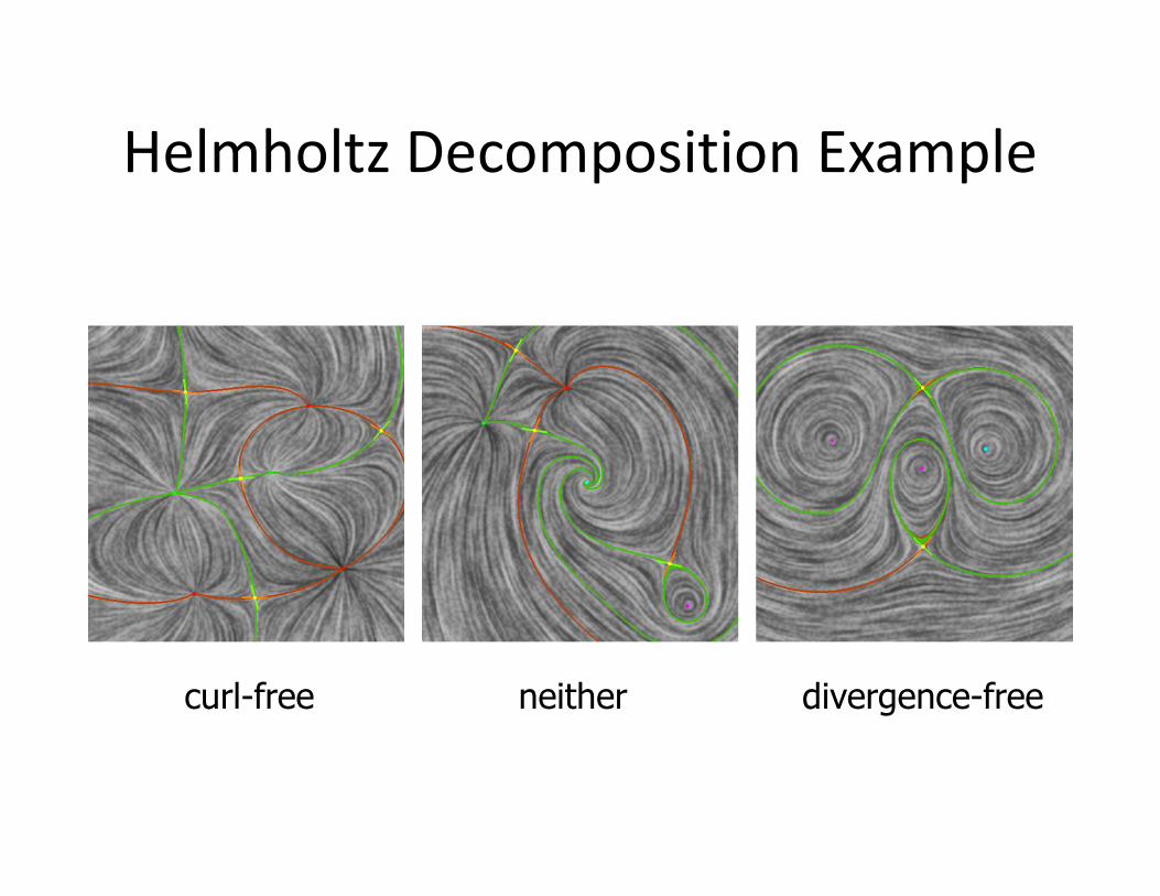
Helmholtz Decomposition Example

curl-free divergence-freeneither

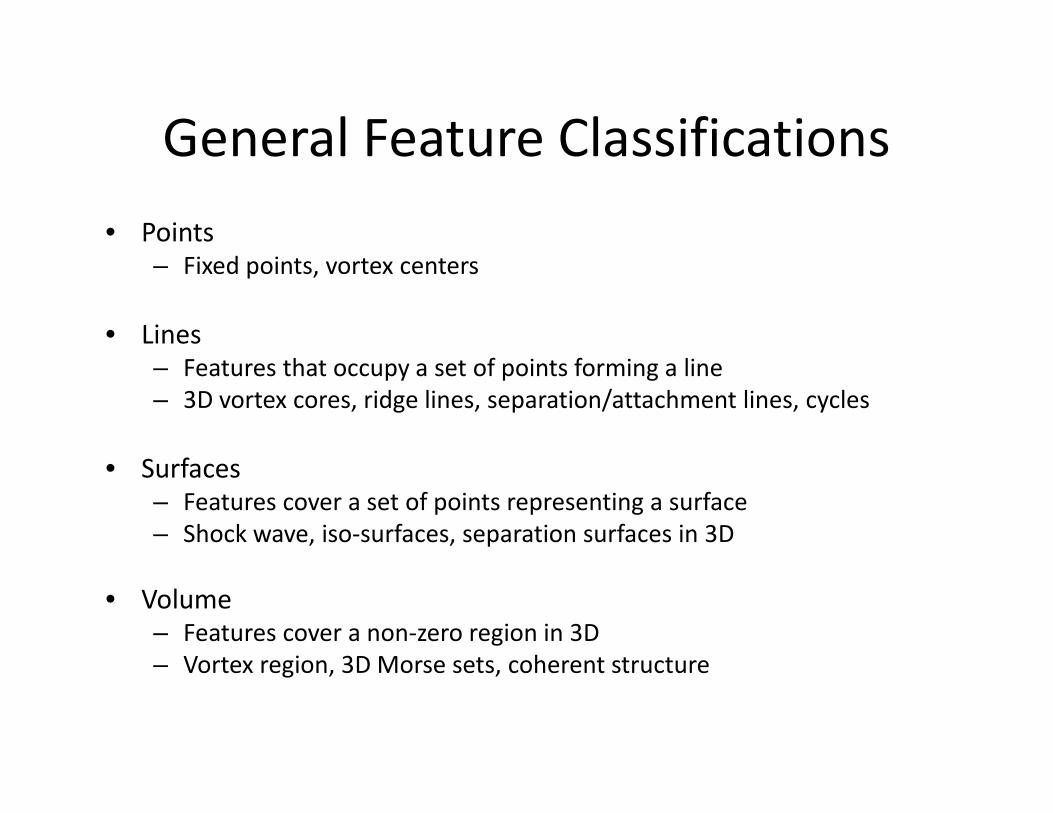
General Feature Classifications

• Points– Fixed points, vortex centers

• Lines– Features that occupy a set of points forming a line

– 3D vortex cores, ridge lines, separation/attachment lines, cycles

• Surfaces– Features cover a set of points representing a surface

– Shock wave, iso-surfaces, separation surfaces in 3D

• Volume– Features cover a non-zero region in 3D

– Vortex region, 3D Morse sets, coherent structure

One important non-topological

features in vector fields is vortex

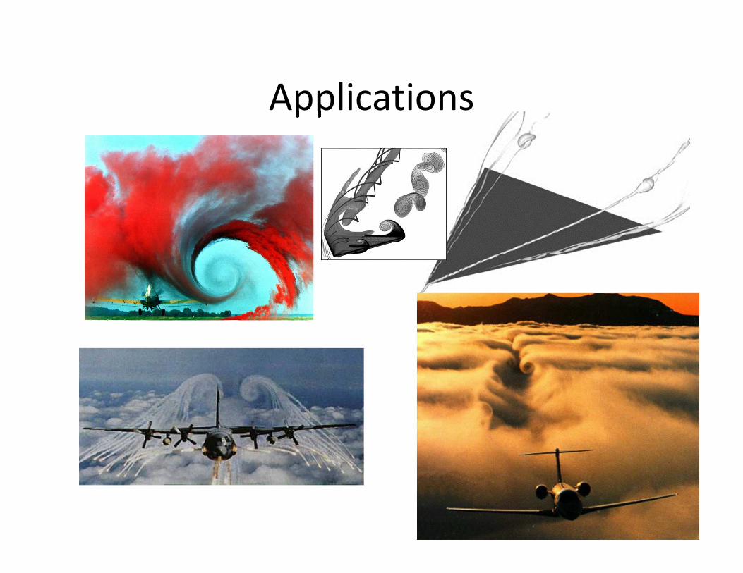
Applications

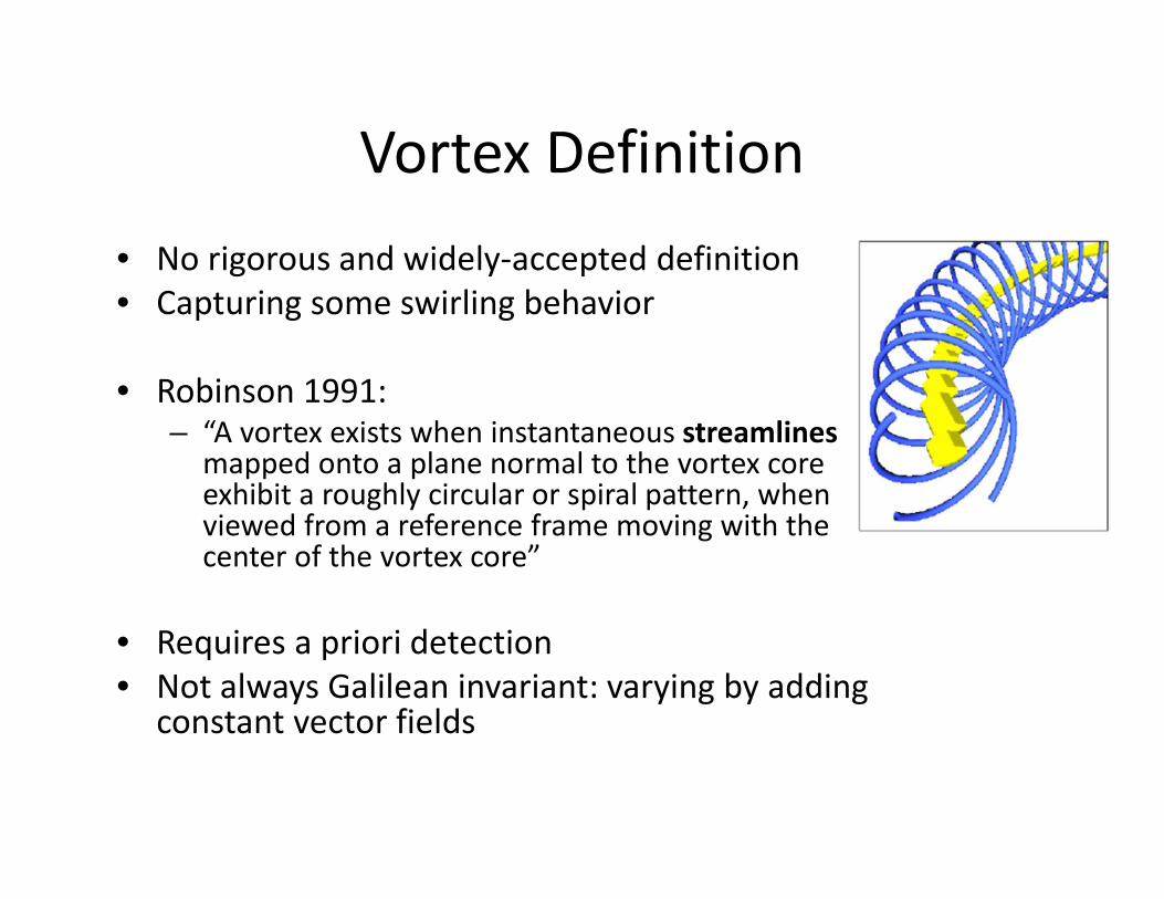
Vortex Definition

• No rigorous and widely-accepted definition

• Capturing some swirling behavior

• Robinson 1991:– “A vortex exists when instantaneous streamlines

mapped onto a plane normal to the vortex core exhibit a roughly circular or spiral pattern, when viewed from a reference frame moving with the center of the vortex core”

• Requires a priori detection

• Not always Galilean invariant: varying by adding constant vector fields

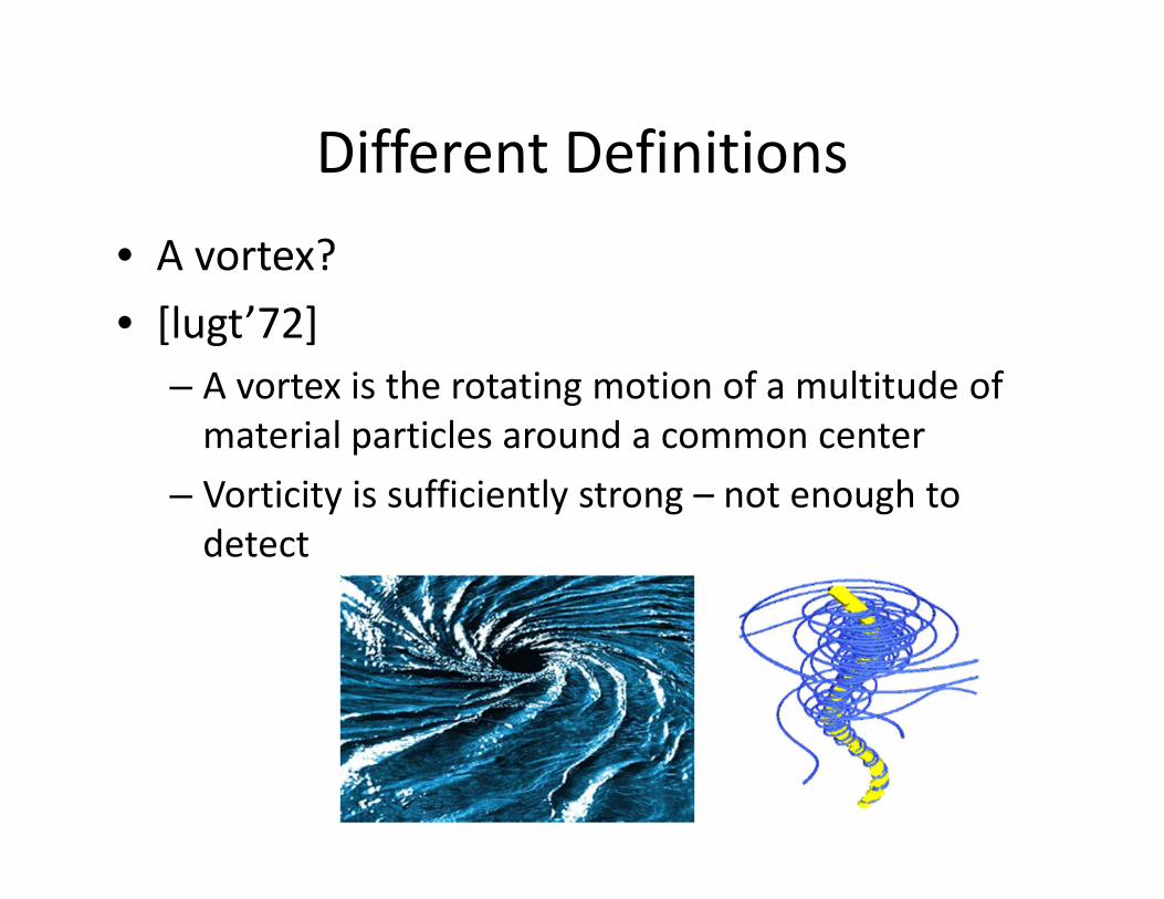
Different Definitions

• A vortex?

• [lugt’72]

– A vortex is the rotating motion of a multitude of

material particles around a common center

– Vorticity is sufficiently strong – not enough to

detect

Different Definitions

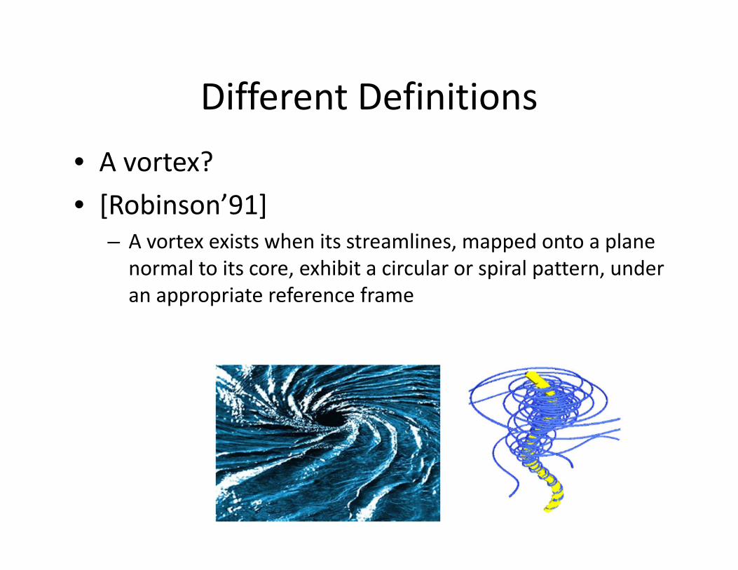
• A vortex?

• [Robinson’91]

– A vortex exists when its streamlines, mapped onto a plane

normal to its core, exhibit a circular or spiral pattern, under

an appropriate reference frame

Different Definitions

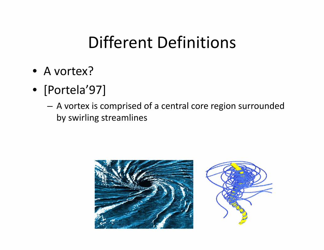
• A vortex?

• [Portela’97]

– A vortex is comprised of a central core region surrounded

by swirling streamlines

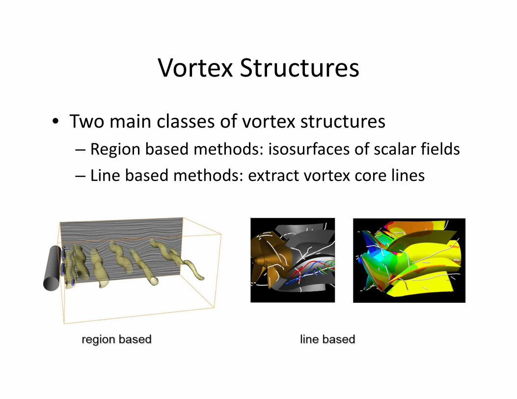
Vortex Structures

• Two main classes of vortex structures

– Region based methods: isosurfaces of scalar fields

– Line based methods: extract vortex core lines

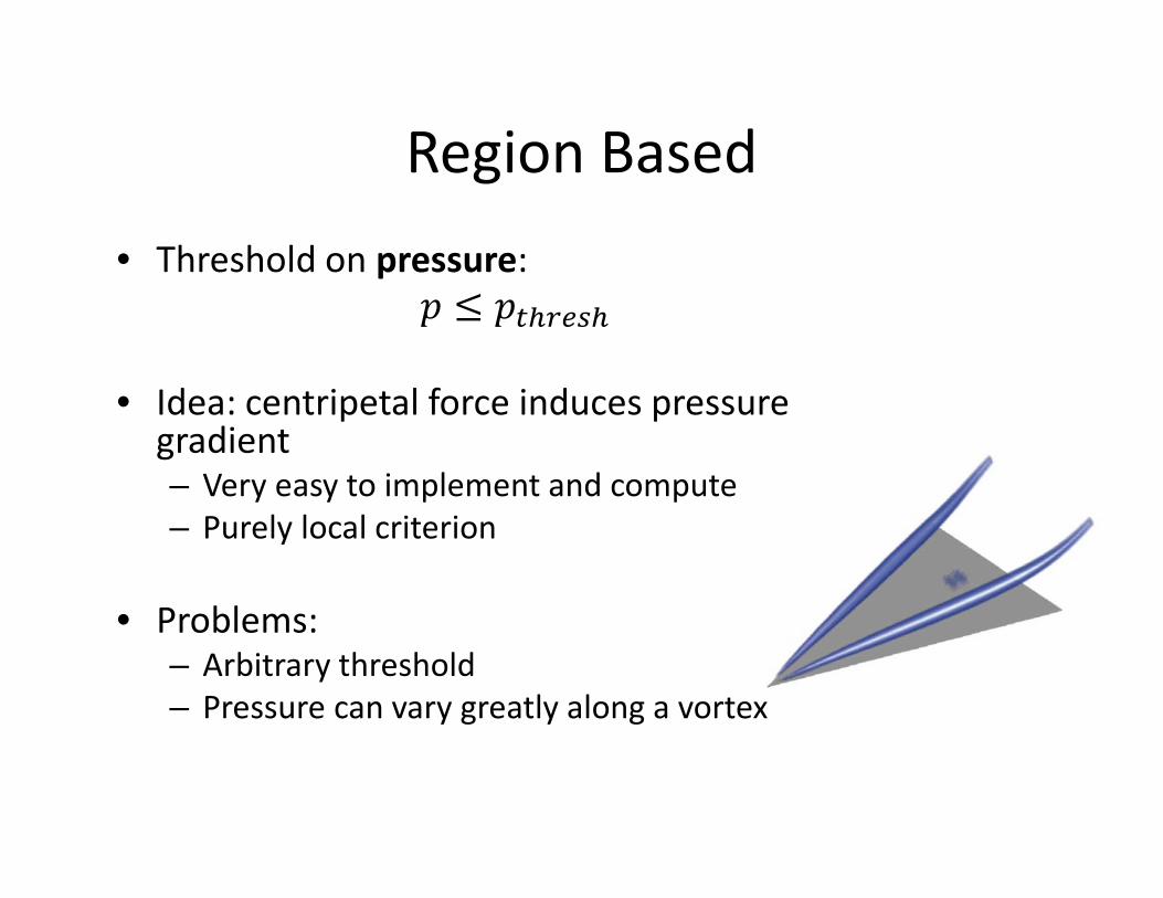
Region Based

• Threshold on pressure:

A B ACDEFGD• Idea: centripetal force induces pressure

gradient– Very easy to implement and compute

– Purely local criterion

• Problems:– Arbitrary threshold

– Pressure can vary greatly along a vortex

Region Based

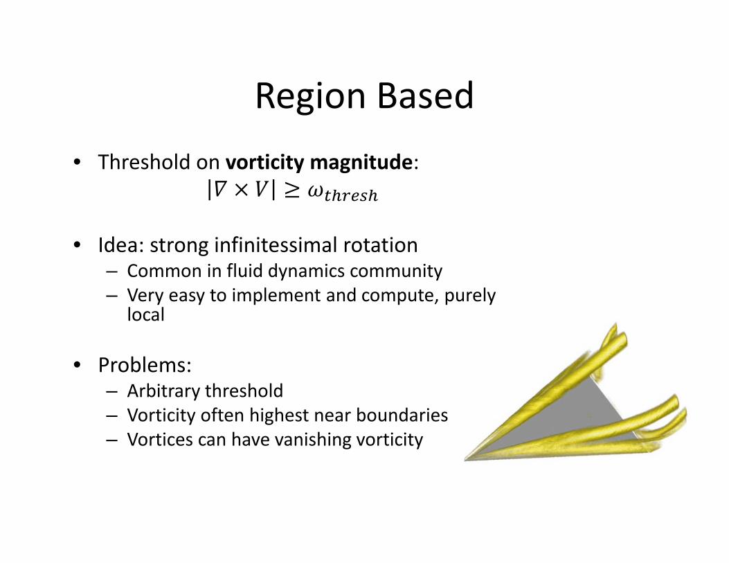
• Threshold on vorticity magnitude:

� × � H ICDEFGD• Idea: strong infinitessimal rotation

– Common in fluid dynamics community

– Very easy to implement and compute, purely local

• Problems:– Arbitrary threshold

– Vorticity often highest near boundaries

– Vortices can have vanishing vorticity

Region Based

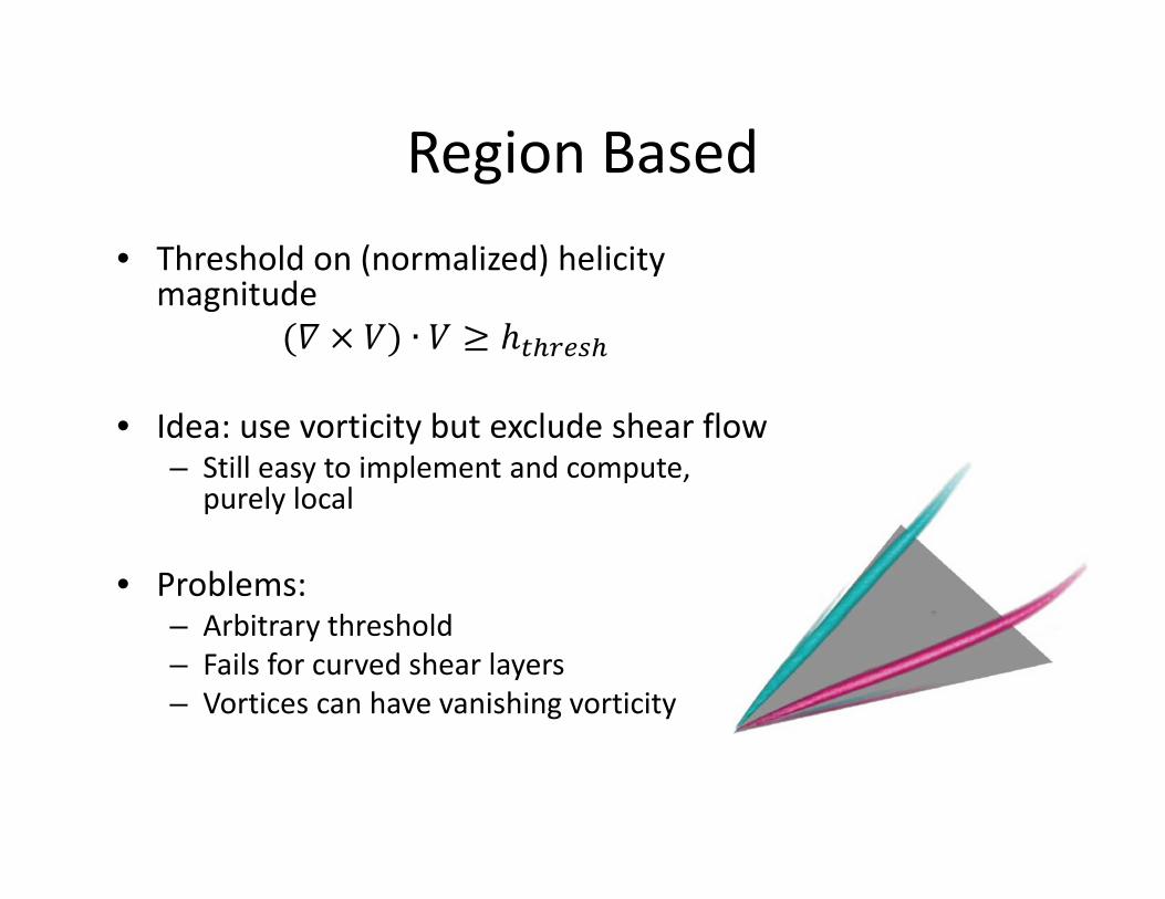
• Threshold on (normalized) helicitymagnitude

(� × �) ∙ � H JCDEFGD• Idea: use vorticity but exclude shear flow

– Still easy to implement and compute, purely local

• Problems:– Arbitrary threshold

– Fails for curved shear layers

– Vortices can have vanishing vorticity

Region Based

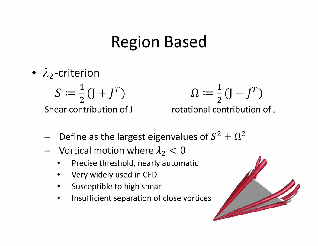
• KL-criterion

M ≔ OL (J + QR) Ω ≔ O

L (J − QR)Shear contribution of J rotational contribution of J

– Define as the largest eigenvalues of ML + ΩL– Vortical motion where KL T 0

• Precise threshold, nearly automatic

• Very widely used in CFD

• Susceptible to high shear

• Insufficient separation of close vortices

Region Based

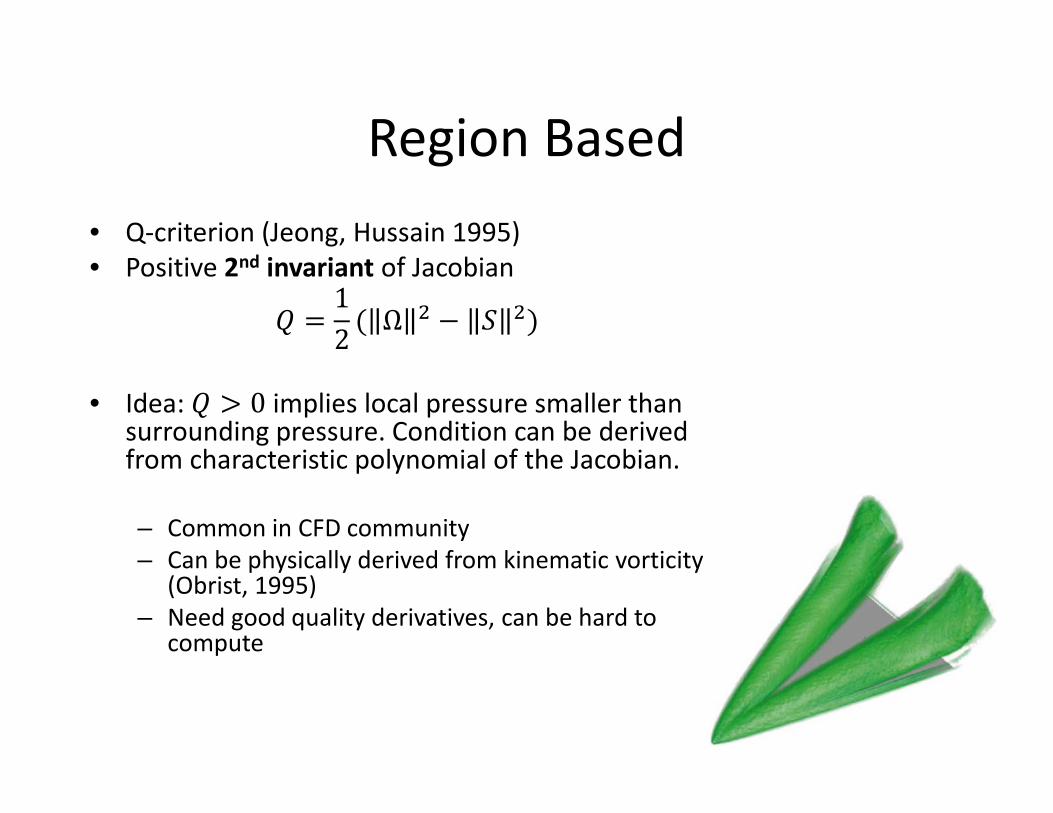
• Q-criterion (Jeong, Hussain 1995)

• Positive 2nd invariant of Jacobian

U = 12 ( Ω L − M L)

• Idea: U X 0 implies local pressure smaller than surrounding pressure. Condition can be derived from characteristic polynomial of the Jacobian.

– Common in CFD community

– Can be physically derived from kinematic vorticity(Obrist, 1995)

– Need good quality derivatives, can be hard to compute

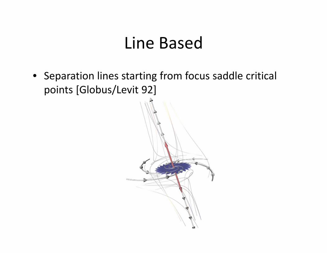
Line Based

• Separation lines starting from focus saddle critical

points [Globus/Levit 92]

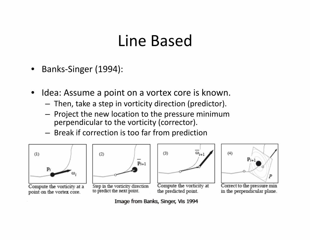
Line Based

• Banks-Singer (1994):

• Idea: Assume a point on a vortex core is known.– Then, take a step in vorticity direction (predictor).

– Project the new location to the pressure minimum perpendicular to the vorticity (corrector).

– Break if correction is too far from prediction

Line Based

• Banks-Singer, continued

• Results in core lines that are roughly vorticitylines and pressure valleys.

– Algorithmically tricky

– Seeding point set can be large (e.g. local pressure minima)

– Requires additional logic to identify unique lines

Line Based

• [Sujudi, Haimes 95]

• In 3D, in areas of 2 imaginary eigenvalues of the Jacobianmatrix: the only real eigenvalue is parallel to V

– In practice, standard method in CFD, has proven successful in a number of applications

– Criterion is local per cell and readily parallelized

– Resulting line segments are disconnected (Jacobian is assumed piecewise linear)

– Numerical derivative computation can cause noisy results

– Has problems with curved vortex core lines (sought-for pattern is straight)

Line Based

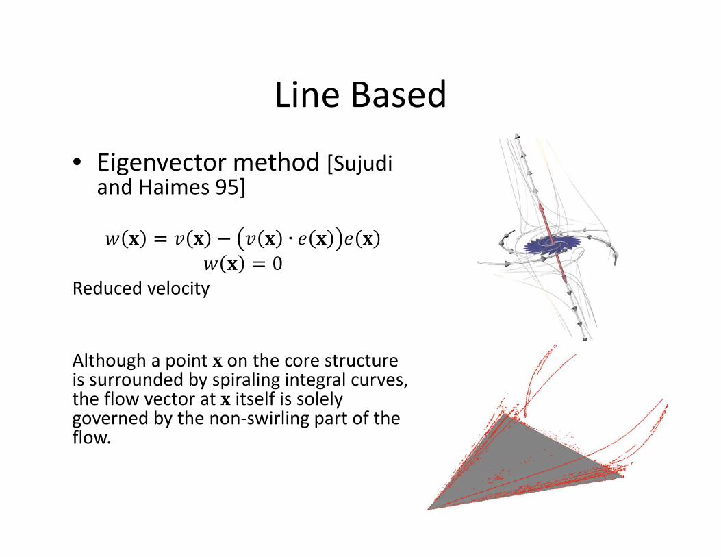
• Eigenvector method [Sujudiand Haimes 95]

Y � = � � − � � ∙ 2 � 2 �Y � = 0

Reduced velocity

Although a point x on the core structure is surrounded by spiraling integral curves, the flow vector at x itself is solely governed by the non-swirling part of the flow.

Line Based

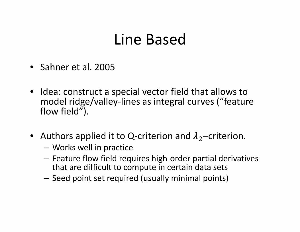
• Sahner et al. 2005

• Idea: construct a special vector field that allows to model ridge/valley-lines as integral curves (“feature flow field”).

• Authors applied it to Q-criterion and KL–criterion.– Works well in practice

– Feature flow field requires high-order partial derivatives that are difficult to compute in certain data sets

– Seed point set required (usually minimal points)

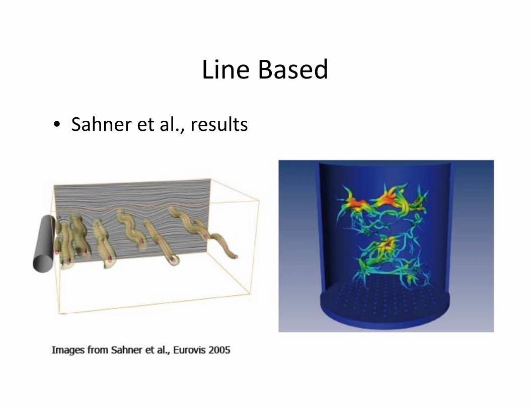
Line Based

• Sahner et al., results

Line Based

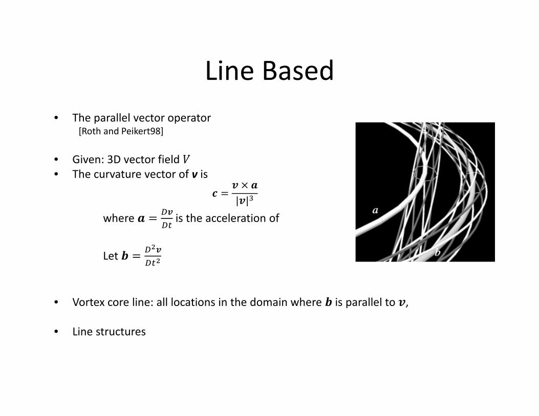
• The parallel vector operator [Roth and Peikert98]

• Given: 3D vector field �• The curvature vector of v is

Z = [ × \|[|^

where \ = _[_C is the acceleration of

Let ` = _a[_Ca

• Vortex core line: all locations in the domain where `is parallel to [,

• Line structures

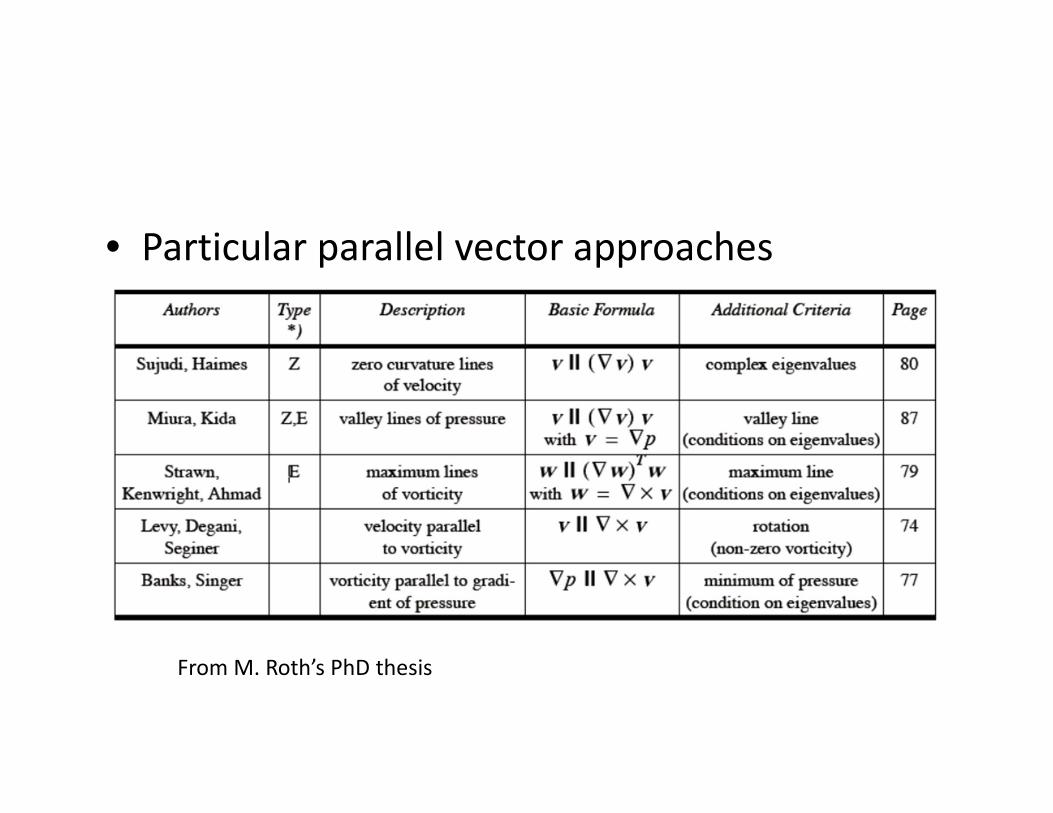
• Particular parallel vector approaches

From M. Roth’s PhD thesis

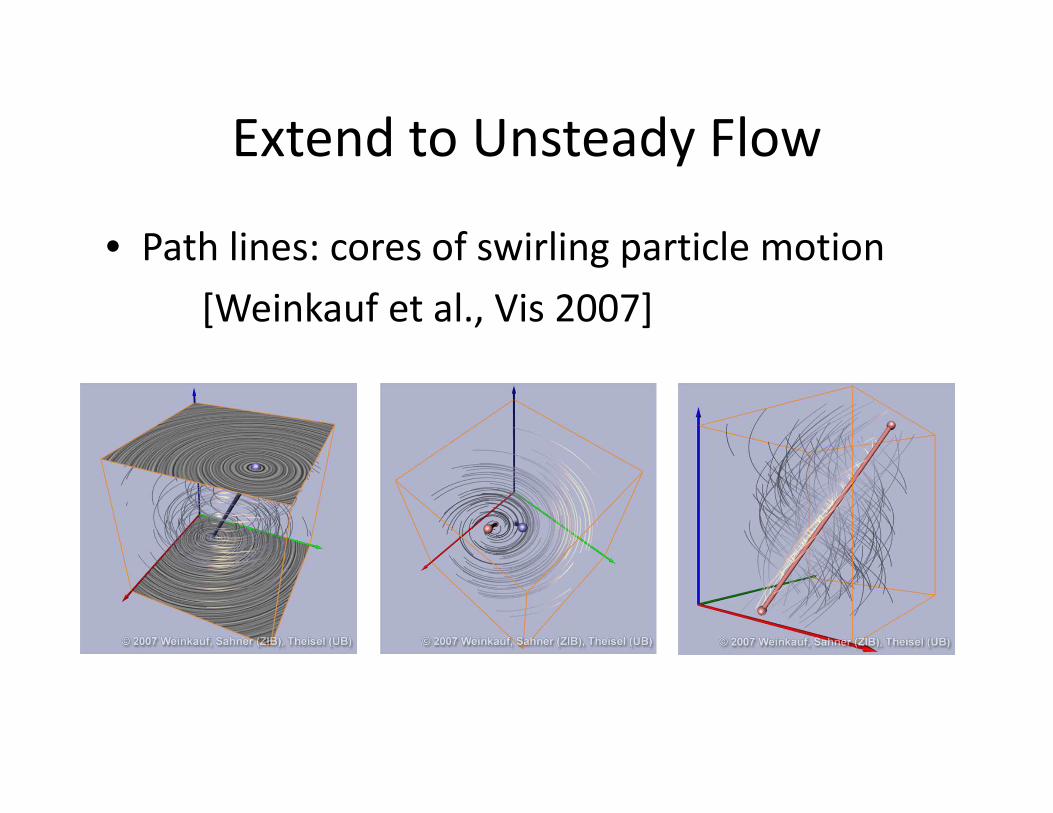
Extend to Unsteady Flow

• Path lines: cores of swirling particle motion

[Weinkauf et al., Vis 2007]

Acknowledgment

• Thanks material from

• Dr. Alexander Wiebel

• Dr. Holger Theisel

• Dr. Filip Sadlo