Embed Size (px)
Citation preview

2
This slide can be downloaded from
● http://www.spcom.ecei.tohoku.ac.jp/~aito/wavelet/slide2.pdf
3
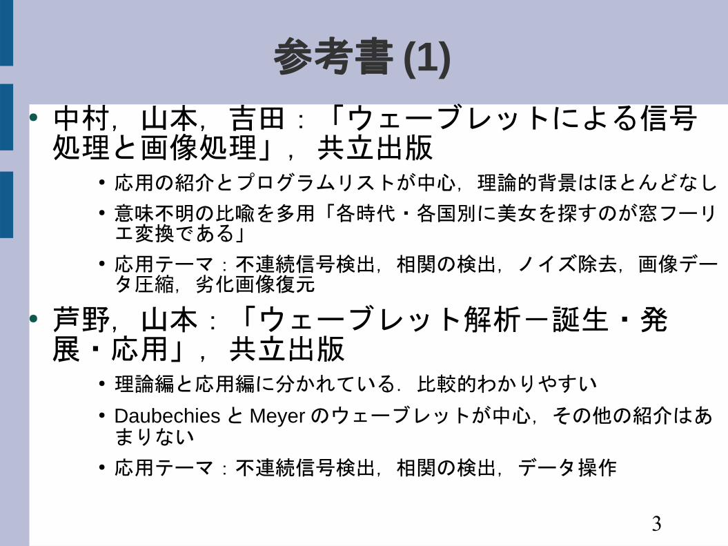
参考書 (1)● 中村,山本,吉田:「ウェーブレットによる信号処理と画像処理」,共立出版
● 応用の紹介とプログラムリストが中心,理論的背景はほとんどなし
● 意味不明の比喩を多用「各時代・各国別に美女を探すのが窓フーリエ変換である」
● 応用テーマ:不連続信号検出,相関の検出,ノイズ除去,画像データ圧縮,劣化画像復元
● 芦野,山本:「ウェーブレット解析-誕生・発展・応用」,共立出版
● 理論編と応用編に分かれている.比較的わかりやすい
● Daubechies と Meyer のウェーブレットが中心,その他の紹介はあまりない
● 応用テーマ:不連続信号検出,相関の検出,データ操作

4
参考書 (2)● 新井:「ウェーブレット解析の基礎理論」森北出版
● 前半が理論,後半が応用だが理論的背景は薄い
● 理論を飛ばして読む目的には良いが,理論をこれだけで理解するのは難しい
● 対象ウェーブレットを幅広く扱っている
● 応用編はプログラムリストつき
● 応用テーマ:エッジ抽出,データ圧縮,積分方程式の数値解法
● C.K.Chui, 桜井・新井訳:「ウェーブレット入門」,東京電機大学出版局
● 理論のみ,応用事例なし
● 理論を概観する章がある.証明抜きで全体像をつかむには良い
● 扱うのはほとんどスプラインウェーブレット.
5
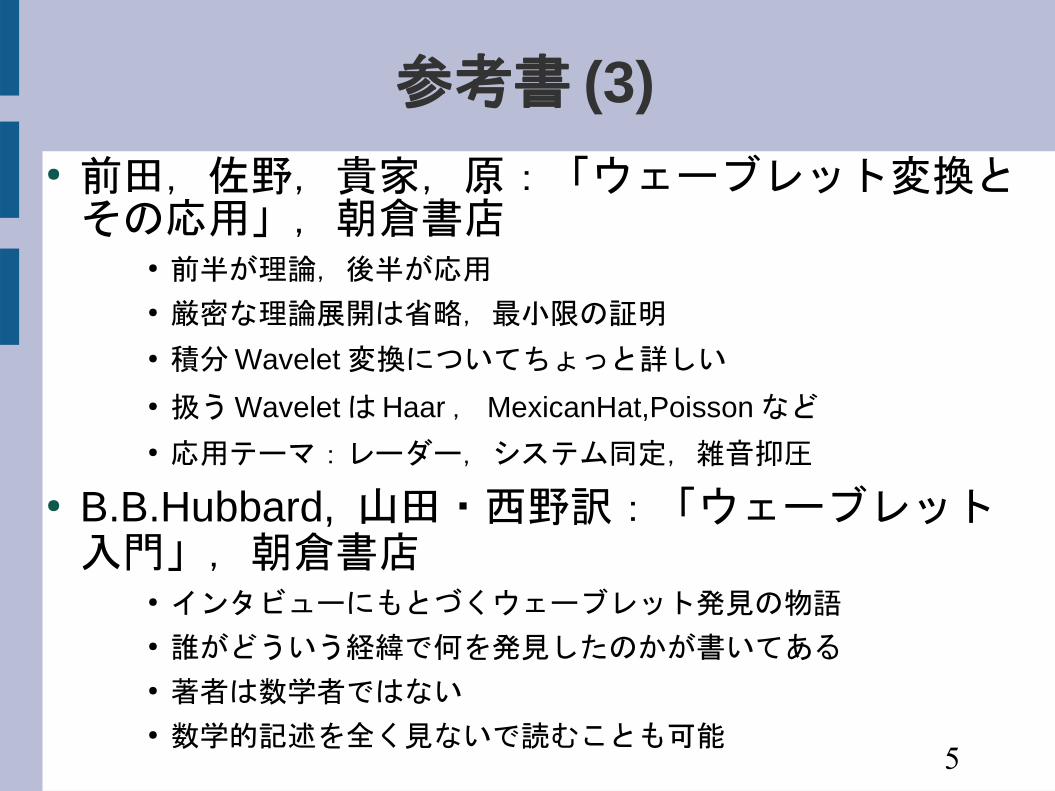
参考書 (3)● 前田,佐野,貴家,原:「ウェーブレット変換とその応用」,朝倉書店
● 前半が理論,後半が応用
● 厳密な理論展開は省略,最小限の証明
● 積分 Wavelet 変換についてちょっと詳しい
● 扱う Wavelet は Haar , MexicanHat,Poisson など
● 応用テーマ:レーダー,システム同定,雑音抑圧
● B.B.Hubbard, 山田・西野訳:「ウェーブレット入門」,朝倉書店
● インタビューにもとづくウェーブレット発見の物語
● 誰がどういう経緯で何を発見したのかが書いてある
● 著者は数学者ではない
● 数学的記述を全く見ないで読むことも可能

6
参考書 (4)● 赤間:「ウェーブレット変換がわかる本」工学社– ウェーブレットの基礎と応用についてわかりやすく解説
– さまざまなウェーブレットを扱う– 理論も比較的詳しいが、わかりやすい感じで書かれている
7
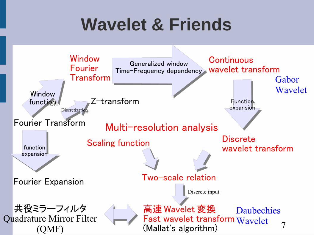
Wavelet & Friends
Fourier Transform
WindowFourierTransform
WindowfunctionWindowfunction
Generalized windowTime-Frequency dependency
Generalized windowTime-Frequency dependency
Continuouswavelet transform
functionexpansion
functionexpansion
Fourier Expansion
Functionexpansion
Functionexpansion
Discrete wavelet transform
Multi-resolution analysis
Scaling function
高速 Wavelet 変換Fast wavelet transform(Mallat's algorithm)
Two-scale relation
Gabor Wavelet
DaubechiesWavelet
共役ミラーフィルタQuadrature Mirror Filter
(QMF)
DiscretizationDiscretization
Z-transform
Discrete input

8
フーリエ変換 Fourier transform● Calculate spectrum from infinite signal
– フーリエ変換 Fourier transform
– フーリエ逆変換 Inverse Fourier transform
f =∫−∞
∞
f x e−i x dx
f x =∫−∞
∞
f xe i x d

9
Analysis of time series● Time-variant spectrum?
Fundamental frequency changes with time● 全体を解析したのでは「だんだん上がる」という分析は不可能

10
Window Fourier Transform● FT of windowed signal
– Analyze temporal change of the signal
F t ,=∫−∞
∞
f xw x−t e−i x dx
=∫−∞
∞
f x ,t x dx

11
Time-Frequency Analysis● Analyze temporal change of the signal by
shifting the window function
12
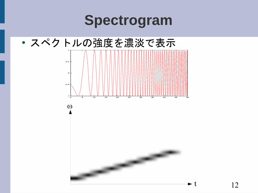
Spectrogram● スペクトルの強度を濃淡で表示
t
w

13
Window Functions● Functions to extract signal of a specific time
– It is desirable to be zero when |t| is large (compact support)
w x =e−t2
2
w x ={121cos t −1t1
0 otherwise
Gaussian
Han (Hanning)

14
Window Functions
w x ={1 −1t10 otherwise
w x ={0.540.46cos t −1t10 otherwise
Hamming
Rectangular

15
Window Functions● Condition of w(x) to be a window function
● Center and width
∫ −∞
∞
∣x w x∣dx∞
∣∣w∣∣2=∫−∞
∞∣w x∣2 dx
x∗= 1
∣∣w∣∣2∫−∞
∞x∣w x∣2dx
Δw=√ 1
||w||2∫−∞
∞(x−x∗)2|w( x)|2 dx

16
Uncertainty of window FT● Longer window → higher frequency resolution
– Two spectral peaks with similar frequencies can be discriminated
● Shorter window → higher temporal resolution– Quick temporal changes can be captured
● Uncertainty– Temporal width × Frequency width > const
(デモプログラム)
17
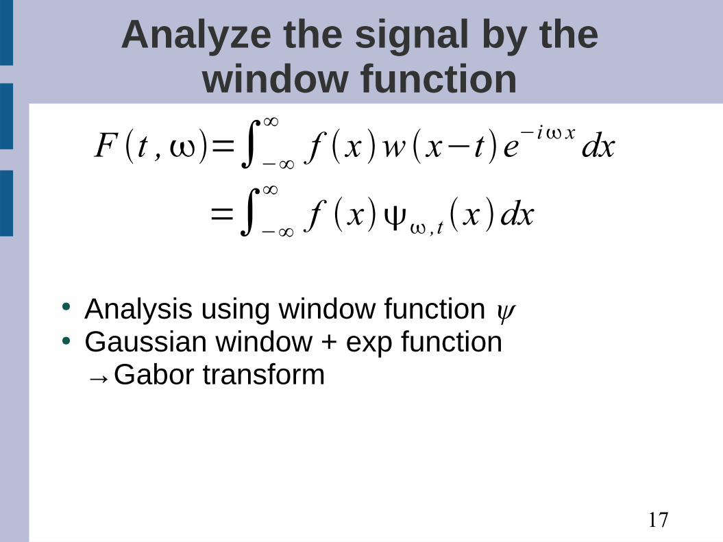
Analyze the signal by thewindow function
● Analysis using window function y● Gaussian window + exp function
→Gabor transform
F t ,=∫−∞
∞f x w x−t e−i x dx
=∫−∞
∞f x ,t x dx

18
Continuous Wavelet transform● Transform using a window function (Wavelet)
– a:周波数の逆数に相当( dilation)– b: 時間に相当( shift)
– :Analyzing wavelet
W f b ,a = 1
a∫−∞
∞f x x−b
a dx

19
Condition of Wavelet● No bias
● Existence of inverse transform
∫−∞
∞ x dx=0
∫−∞
∞ ∣ x ∣2
∣x∣dx=1
2C∞
20
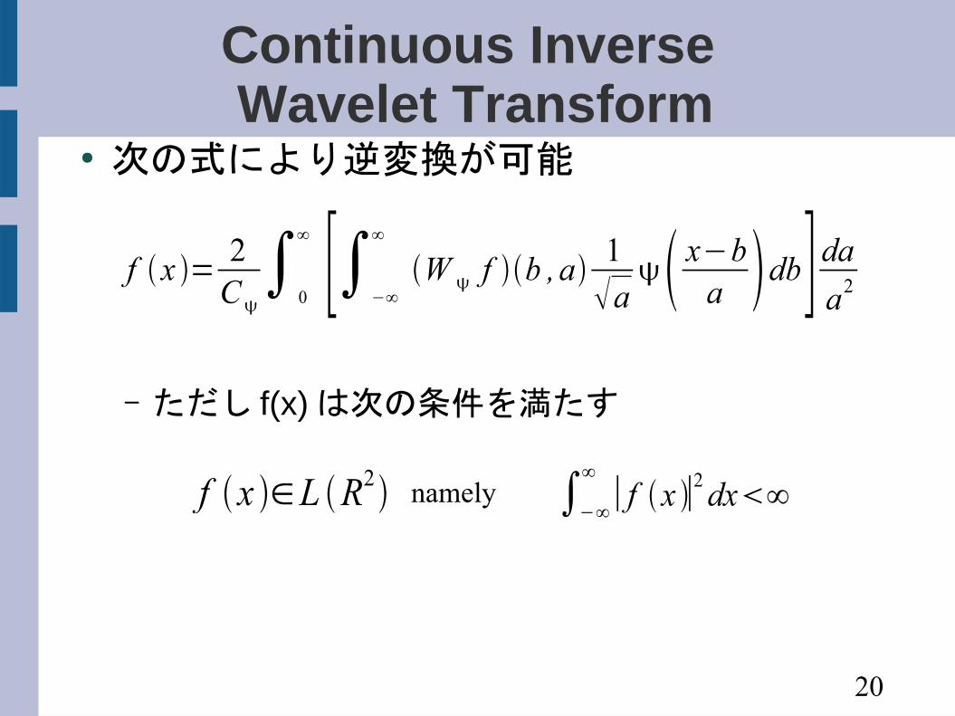
Continuous Inverse Wavelet Transform
● 次の式により逆変換が可能
– ただし f(x) は次の条件を満たす
f x = 2C∫
0
∞ [∫−∞
∞
W f b ,a 1
a x−b
a db] da
a2
f x ∈L R2 namely ∫−∞
∞∣ f x ∣2 dx∞

21
Examples of Analyzing Wavelet
● Haar wavelet
● Mexican hat wavelet
x={ 0 x01 0≤ x0.5−1 0.5≤ x10 1x
x=1− x2e− x2
2

22
Exercise● cos(kx) を Haar で Wavelet 変換してみよう
● こんな風になるはず– 下の図では a は対数スケールであることに注意
– a は周波数の逆数→ k が大なら a は小
23
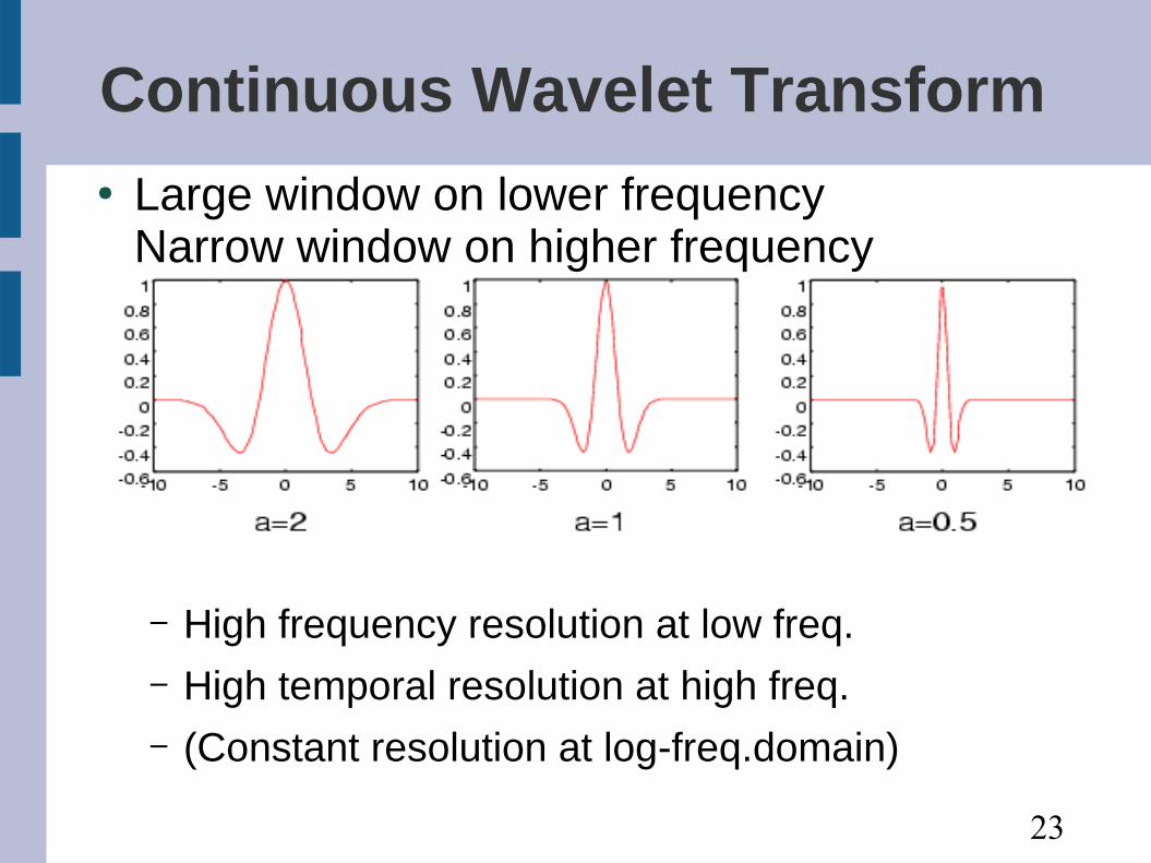
Continuous Wavelet Transform● Large window on lower frequency
Narrow window on higher frequency
– High frequency resolution at low freq.– High temporal resolution at high freq.– (Constant resolution at log-freq.domain)

24
Discrete Wavelet Transform● CWT:1 variable→2 variables
● Express the original function by summing all coefficients→Discrete Wavelet Transform (Wavelet Expansion)
W f b , a = 1
a∫−∞
∞f x x−b
a dx
f x =∑j=−∞
∞
∑k=−∞
∞
W f k2 j ,
12 j 2 j/2 2 j x−k
= ∑j=−∞
∞
∑k=−∞
∞
W f k2 j ,
12 j jk x
CONSTANT

25
Wavelet Coefficients● Constant part
● The coefficients are values of CWT at discrete points
c jk=W f k
2 j,
1
2 j f x =∑
j=−∞
∞
∑k=−∞
∞
c jk jk x
LetWaveletcoefficients

26
Notes on the Wavelet Coefficients
● a is in proportion to inverse of freq.– Sampling points at a-b domain
– Sampling points at f=1/a-b domain

27
Wavelet basis function(1)● Wavelet expansion is a kind of 2-D function
expansion
● Cf.– Taylor-McLaurin expansion
– Fourier expansion
● is the basis function of Wavelet expansion
f x =∑j=−∞
∞
∑k=−∞
∞
c jk jk x
f x = ∑k=−∞
∞
ak x k
f x = ∑k=−∞
∞
ak e−ikx
ψ jk (x)

28
Wavelet basis function(2)● Basis functions
– Any function (under a certain conditions) can be composed by a (infinite) weighted sum of the basis functions
– It does not necessarily guarantee uniqueness of coefficients
● Orthonormal basis functions
– Uniquely expands any function
– yjk
based on Haar function is the simplest orthonormal basis
∫−∞
∞ jk x j ' k ' x dx= jj ' kk '
∫−∞
∞2 j /2H 2
j x−k 2 j ' /2H 2j ' x−k dx= jj ' kk '
29
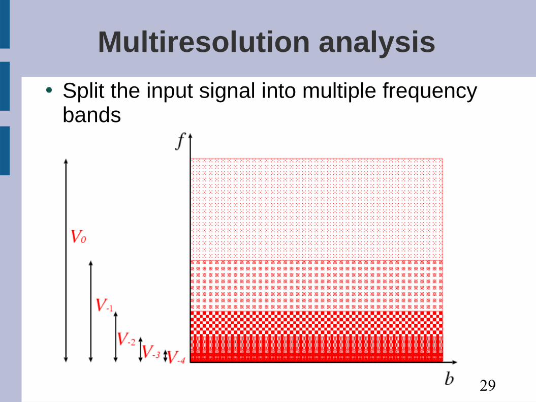
Multiresolution analysis● Split the input signal into multiple frequency
bands

30
Multiresolution Analysis● Relations between the function classes
● Orthonormal basis of V0 Scaling function
● The simplest scaling function
⊂V−2⊂V −1⊂V 0⊂V 1⊂V 2⊂
f ∈V 0f x = ∑
k=−∞
∞
ck x−k
H x={1 0≤x10 otherwise O
1
1

31
Signal Decomposition using the Scaling function
● What functions are expressed by ? – For any integer k,
then
A function sampled at the integral points
k≤x<k+1 f (x)= f (k )
ϕ H (x)
32
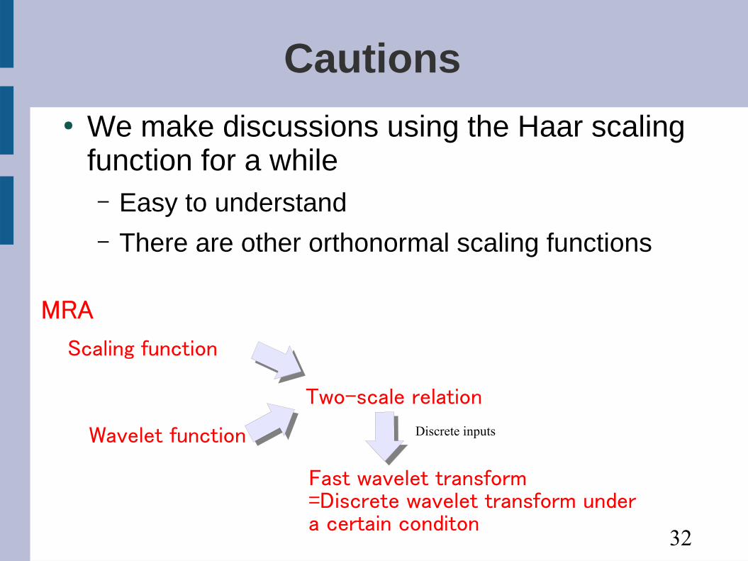
Cautions● We make discussions using the Haar scaling
function for a while– Easy to understand– There are other orthonormal scaling functions
Wavelet function
MRA
Scaling function
Fast wavelet transform=Discrete wavelet transform under a certain conditon
Two-scale relation
Discrete inputs

33
Signal Decomposition using the Scaling function
● Decomposition using the scaling function
●Express the original signal as a weighted-sum of the scaling functions
c−6H x6
c−5H x5
c−4H x4
c−3H x3
⋮

34
Various Scales
O1
1 O1
1 O1
1
H xH 0.5x H 2x
f x ∈V−1 f x ∈V 0 f x ∈V 1

35
Composition of Scaling Function
● Compose the coarse scaling function using the fine scaling functions
● Haar scaling function
x= ∑k=−∞
∞
pk2x−k
H x=H 2x H 2x−1
O
1
1=
O
1
1 O
1
1+
p0=1, p1=1 pk=0 k≠0, k≠1

36
Decomposition of scaling function
x∈V 1−V 0
x=∑−∞
∞
qk2x−k
V 1V 0
W 0
Basis function ϕ(2 x−k )
ϕ (x−k )
ψ(x−k )

37
Decomposition of scaling functon
● Relations between ϕ (x ) , ψ(x) , ϕ (2 x )
ψ (x )=∑−∞
∞
qk ϕ (2 x−k )
ϕ ( x)=∑−∞
∞
pk ϕ (2 x−k ) two-scale relation
Haar scaling function
ϕ ( x)=ϕ (2 x )+ϕ (2 x−1)ψ (x )=ϕ (2 x)−ϕ (2 x−1)
x :Haar wavelet function
qk=−1k p1−k
38
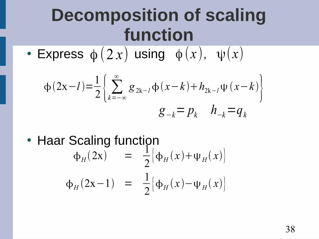
Decomposition of scaling function
● Express using
● Haar Scaling function
ϕ (2 x) ϕ (x ) , ψ(x)
2x−l =12 {∑k=−∞
∞
g 2k−lx−k h2k−l x−k }g−k= pk h−k=qk
H 2x = 12{H x H x}
H 2x−1 = 12{H x −H x}

39
Notes
● The function j is not necessarily a mother wavelet even when it is an orthonormal basis of W
0
– Other condition is needed such as
– Composition/decomposition of scaling function is STRONGLY related to the discrete wavelet
–
∫−∞
∞ ∣ x ∣2
∣x∣dx=1
2C∞
40
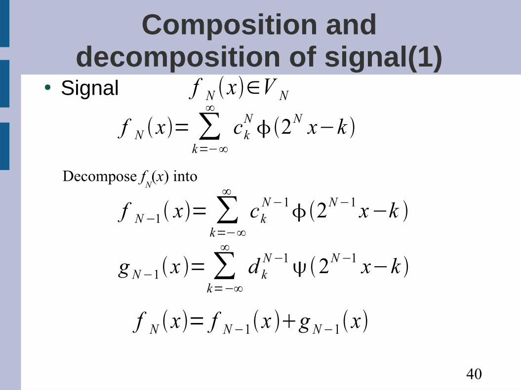
Composition and decomposition of signal(1)
● Signal f N x∈V N
f N x= ∑k=−∞
∞
ckN2N x−k
Decompose fN(x) into
f N−1 x= ∑k=−∞
∞
ckN−12N−1 x−k
g N−1x =∑k=−∞
∞
d kN−12N−1 x−k
f N x= f N−1x g N−1x

41
Composition and decomposition of signal(2)
● Relations among – Decomposition
– Composition
c N , cN−1 , d N−1
ckN−1=
12∑
l
c lN g2 k− l=
12∑
l
c lN p l−2 k
d kN−1=
12∑
l
c lN h2 k−l=
12∑
l
clN ql−2 k
ckN=∑
l{cl
N−1 pk−2ld lN−1 qk−2l}

42
Composition and decomposition of signal(3)
● In case of the Haar's scaling function– Decomposition
– Composition
ckN−1=1
2c2k
N c2k1N d k
N−1=12c2k
N −c2k1N
c2kN−1=ck
N−1d kN−1 c2k1
N−1=ckN−1−d k
N−1
f N x=∑k
ckN H 2
N x−k
Average of two contiguous points
Half of the difference of two contiguous points
f N−1 x=∑k
ckN−1H 2
N−1 x−k f N−1 x=∑k
d kN−1H 2
N−1 x−k
43
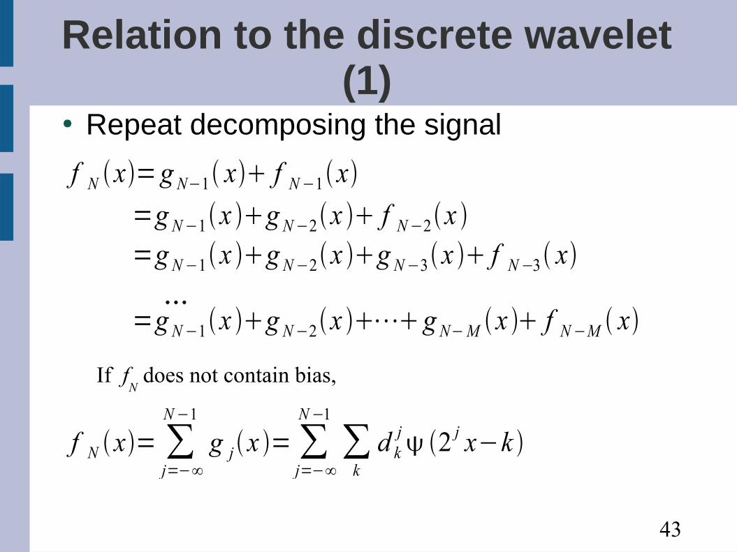
Relation to the discrete wavelet (1)
● Repeat decomposing the signal
f N x=g N−1 x f N−1x=g N−1x g N−2x f N−2x =g N−1x g N−2x g N−3x f N−3 x
...=g N−1x g N−2x ⋯g N−M x f N−M x
If fN does not contain bias,
f N x= ∑j=−∞
N−1
g jx =∑j=−∞
N−1
∑k
d kj 2 j x−k

44
Relation to the discrete wavelet(2)
Decomposition of the signal
Discrete wavelet transform
f N x= ∑j=−∞
N−1
∑k
d kj2 j x−k
f N x= ∑j=−∞
N−1
∑kW f N k
2 j ,12 j 2 j /2 2 j x−k
As the coefficients of orthonormal basis functions are unique,
d kj=W f N k
2 j,
1
2 j 2 j /2
Decompositon using the scaling function = Discrete wavelet transform

45
Fast Wavelet Transform
● Discrete wavelet transform of fN
– When using the Haar's scaling functionfN :piecewise constant function at 2-N interaval
● Sampled signal can be regarded as fN
Fast ⇒ Wavelet Transform (Mallat's algorithm)

46
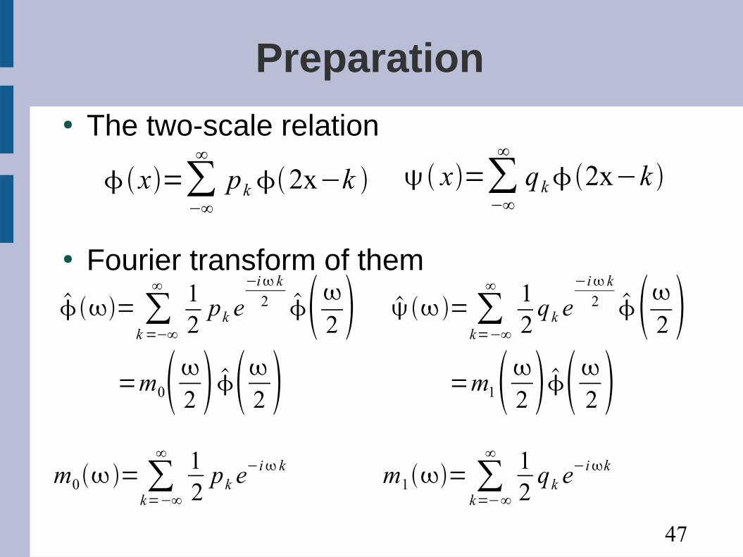
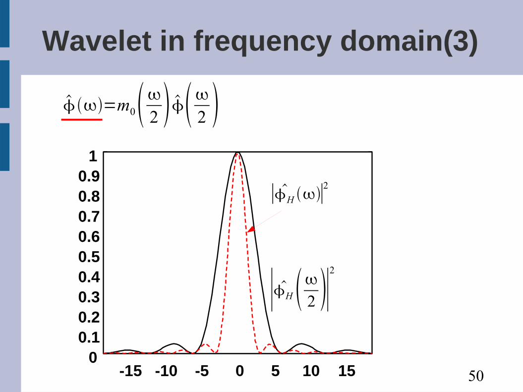
Wavelet in frequency domain● The two-scale relation: time domain● The scaling function in frequency domain
– Higher-order fN: Large bandwidth,
Narrow support
– Lower-order fN: Narrow bandwidth,
Wide support
– yN
compensatesfN
fN
fN+1 y
N
47
Preparation● The two-scale relation
● Fourier transform of them
x=∑−∞
∞
qk2x−k x=∑−∞
∞
pk 2x−k
= ∑k=−∞
∞ 12
pk e−i k
2 2 =m02 2
=∑k=−∞
∞ 12
qk e−i k
2 2 =m12 2
m0=∑k=−∞
∞ 12
pk e−i k m1= ∑k=−∞
∞ 12
qk e−ik

48
Wavelet in frequency domain(1)
=m02 2
0 0.1 0.2 0.3 0.4 0.5 0.6 0.7 0.8 0.9
1
-15 -10 -5 0 5 10 15
∣ H 2 ∣2
=∣1−e−i/2
i/2 ∣2
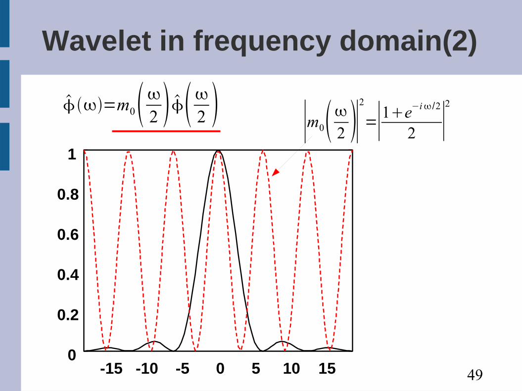
49
Wavelet in frequency domain(2)
=m02 2
0
0.2
0.4
0.6
0.8
1
-15 -10 -5 0 5 10 15
∣m02 ∣2
=∣1e−i/2
2 ∣2
50
Wavelet in frequency domain(3)
0 0.1 0.2 0.3 0.4 0.5 0.6 0.7 0.8 0.9
1
-15 -10 -5 0 5 10 15
∣ H ∣2
=m02 2
∣ H 2 ∣2

51
Wavelet in frequency domain(4)
=m12 2
0 0.1 0.2 0.3 0.4 0.5 0.6 0.7 0.8 0.9
1
-15 -10 -5 0 5 10 15
m12 =1−e−i/2
2
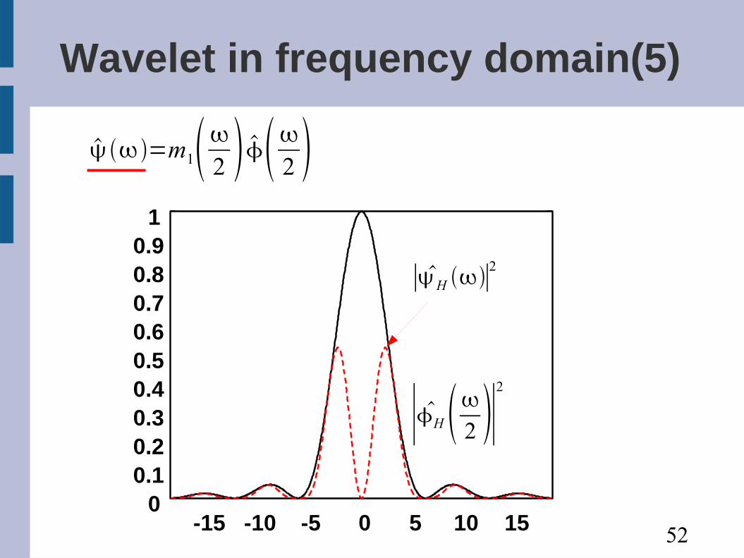
52
Wavelet in frequency domain(5)
=m12 2
0 0.1 0.2 0.3 0.4 0.5 0.6 0.7 0.8 0.9
1
-15 -10 -5 0 5 10 15
∣ H ∣2
∣ H 2 ∣2

53
Wavelet as filters● m
0:Low-pass filter,
m
1:High-pass filter
0
0.2
0.4
0.6
0.8
1
0 0.5 1 1.5 2 2.5 3
m1m0 QuadratureMirrorFilter(QMF)
54
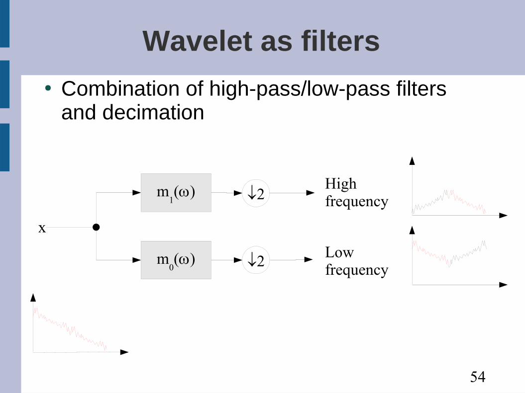
Wavelet as filters● Combination of high-pass/low-pass filters
and decimation
m1(w)
m0(w)
x
2
2
High frequency
Lowfrequency

55
Wavelet other than Haar
● Many kinds of mother wavelets are proposed– Continuous Wavelet Transform:
Gabor, Maxican hat, ...– Discrete Wavelet Trasform:
Spline, Daubechies, Meyer,...
56
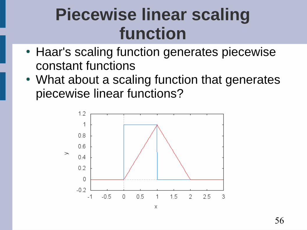
Piecewise linear scaling function
● Haar's scaling function generates piecewise constant functions
● What about a scaling function that generates piecewise linear functions?

57
Piecewise linear scaling function
● This scaling function generates piecewise linear functions, but not orthogonal

58
Piecewise linear scaling function
● Two-scale relation
ϕ(x)=ϕ(2 x)+ 2ϕ(2 x−1)+ ϕ(2 x−2)ψ( x)=−ϕ(2 x)+ 2ϕ(2 x−1)−ϕ(2 x−2)

59
Piecewise linear scaling function
● The previous scaling function/wavelet function are not orthonormal
Cannot be used as a mother wavelet⇒● Can we generate an orthonormal wavelet
from these scaling/wavelet functions?● Answer: the Battle-Lemarié wavelet
60
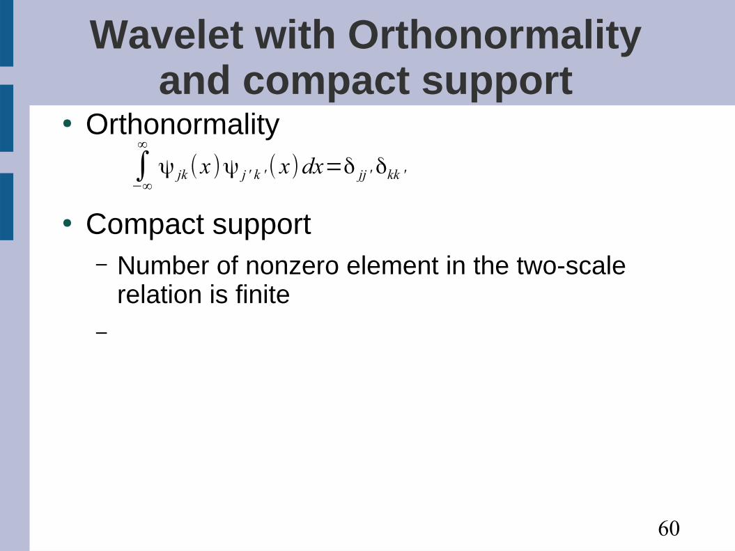
Wavelet with Orthonormality and compact support
● Orthonormality
● Compact support– Number of nonzero element in the two-scale
relation is finite–
∫−∞
∞
ψ jk (x)ψ j ' k ' ( x)dx=δ jj ' δkk '

61
Daubechies' Wavelet (2nd order)● Two-scale relation
● f and j cannot be expressed by analytical functions
x =138
2x338
2x−1 3−38
2x−21−38
2x−3
x=1−38
2x−3−38
2x−1338
2x−2−138
2x−3
x x

62
Daubechies' Wavelet in frequency domain
● Daubeches' wavelet as a filter
m0 =138
338
e−i3−38
e−2i1−38
e−3i
0
0.2
0.4
0.6
0.8
1
0 0.5 1 1.5 2 2.5 3
Haar Daubechies(2)
Sharper than the Haar's wavelet

63
Daubechies' higher-orderwavelet
-2
-1.5
-1
-0.5
0
0.5
1
1.5
0 0.5 1 1.5 2 2.5 3
Daubechies 4 tap wavelet
scaling functionwavelet function
0
0.2
0.4
0.6
0.8
1
1.2
0 0.5 1 1.5 2 2.5 3 3.5 4
D4 wavelet - Fourier amplitudes
scaling functionwavelet function
From Wikipedia, the free encyclopedia

64
Vanishing Moment● The n-th Moment of function f
● The function has A vanishing moment↔
● Wavelet ψ has A vanishing moment=Scaling function φ can express piece-wise xA-1 function
● The 2n-tap Daubechies wavelet function has n vanishing moment
M n( f )=∫−∞
∞
xn f (x)dxM n( f )=∫−∞
∞
xn f (x)dx
M 0( f )=M 1( f )=⋯=M A−1( f )=0

65
Vanishing Moment● Example
– Haar wavelet has 1 vanishing moment
– Thus it can express a piecewise-constant (x0) signal
M 0(ψ H)=∫ψ H (x )dx=∫0
1/2
1dx−∫1/2
1
1dx=0

66
Vanishing Moment
Wavelet Vanishing moment
Explanation
D2 (Haar) 1 Piecewise constant (x0)
D4 2 Piecewise linear (x1)
D6 3 Piecewise quadratic (x2)
D8 4 Piecewise cubic (x3)
https://www.dsprelated.com/showarticle/1006.php

67
Other wavelets
● Simlet ● Coiflet ● Biorthogonal wavelet
–CDF wavelet

68
Symlet● Orthogonal wavelet designed by I. Daubachies● Orthogonal and has compact support
– 2 to 6 tap symlet is identical to Daubecies wavelet– Wavelet functions of 2n-tap Symlet have n vanishing
moment● Function is nearly symmetric
20-tap Symlet 20-tap Daubechies松嶋他「 AIC によるウェーブレット基底関数の選択」,応用統計学 33(2)201-219, 2004
69
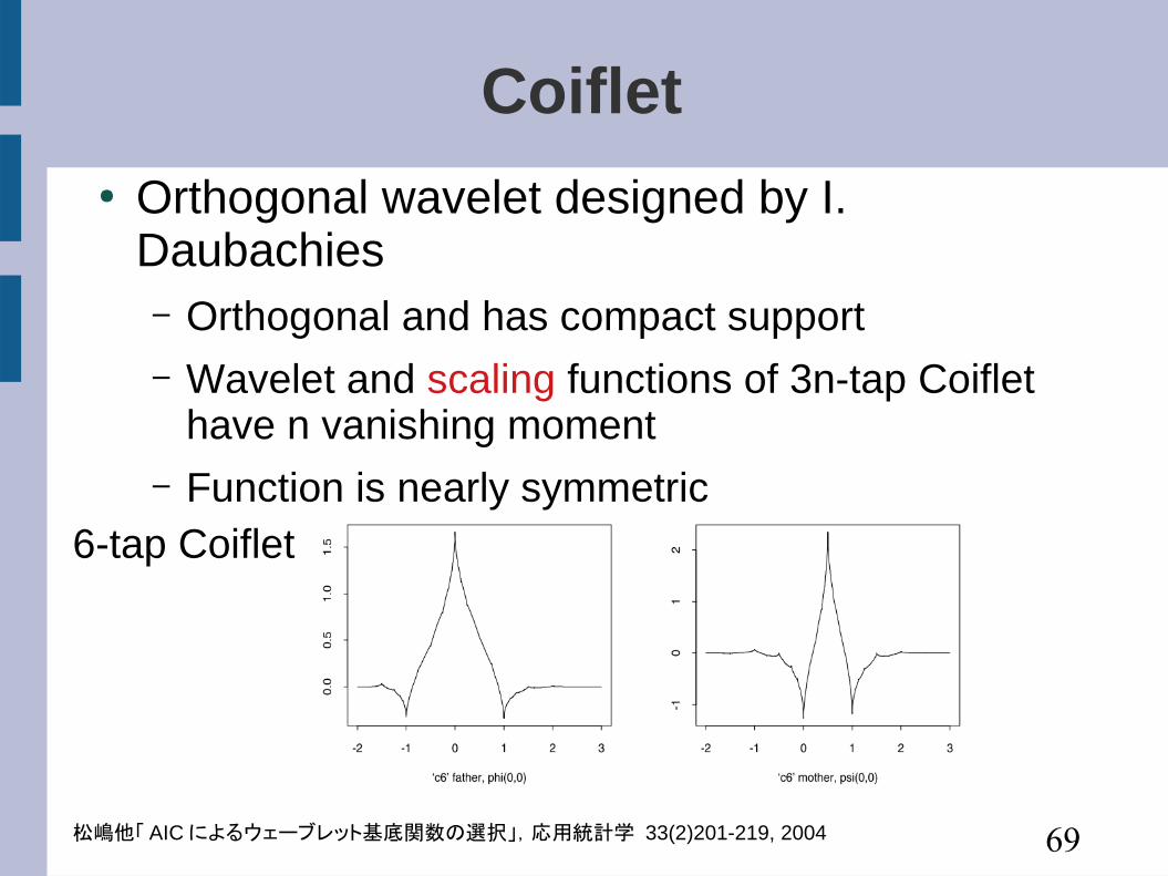
Coiflet● Orthogonal wavelet designed by I.
Daubachies– Orthogonal and has compact support– Wavelet and scaling functions of 3n-tap Coiflet
have n vanishing moment– Function is nearly symmetric
6-tap Coiflet
松嶋他「 AIC によるウェーブレット基底関数の選択」,応用統計学 33(2)201-219, 2004

70
Biorthogonal wavelet● Orthogonal wavelet
– It is impossible to design an orthogonal wavelet that has compact support and the function is symmetric.
● Biorthogonal (双直交)wavelet– Use of different filters for analysis and synthesis– Biorthogonality
∫ψ jk (x)ψ j ' k' (x)dx=δ j j 'δ k k '
∫ψ jk(x)~ψ j ' k' (x)dx=δ j j 'δ k k '

71
Biorthogonal Wavelet● Uniqueness of wavelet coefficient
– Orthogonal wavelet
– Biorthogonal wavelet
f ( x)=∑j∑k
c jkψ jk ( x)
∫ψ jk (x) f ( x)dx=∫ψ jk(x)∑j∑k
c jkψ jk( x)dx=c jk
∫~ψ jk (x) f ( x)dx=∫~ψ jk(x)∑j∑k
c jkψ jk( x)dx=c jk

72
CDF wavelet● Cohen-Daubechies-Feauveau wavelet
– Biorthogonal– Compact support, symmetric– LPF and HPF have different tap length– CDF 5/3 wavelet (used in JPEG2000)
http://wavelets.pybytes.com/wavelet/bior2.2/
73
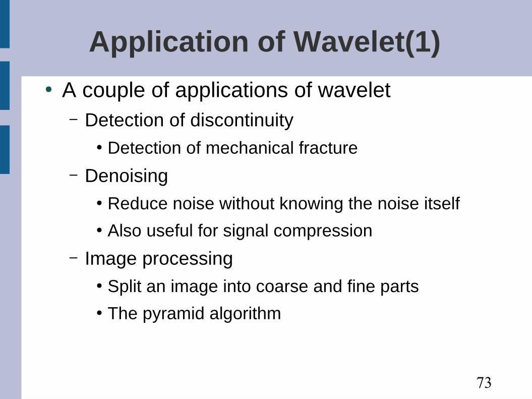
Application of Wavelet(1)● A couple of applications of wavelet
– Detection of discontinuity● Detection of mechanical fracture
– Denoising● Reduce noise without knowing the noise itself● Also useful for signal compression
– Image processing● Split an image into coarse and fine parts● The pyramid algorithm
74
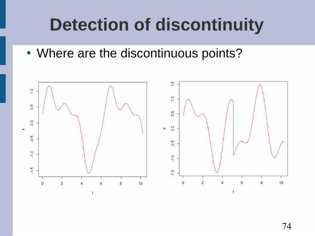
Detection of discontinuity● Where are the discontinuous points?
75
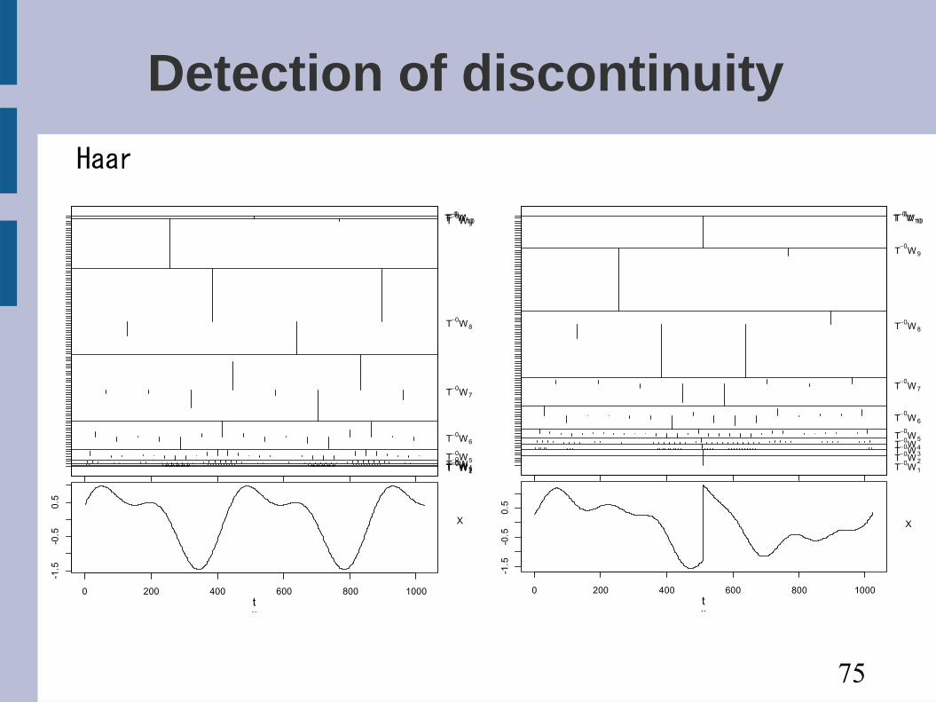
Detection of discontinuity
Haar
0 200 400 600 800 1000
-1.5
-0.5
0.5
x
X
t
T0W1T0
W2T0W3T
0W4
T0W5
T0W6
T0W7
T0W8
T0
W9T0W10T0V10
0 200 400 600 800 1000
-1.5
-0.5
0.5
x
X
t
T0W 1
T0W 2
T0W 3T0W 4
T0
W 5
T0
W 6
T0
W 7
T0W 8
T0
W 9
T0W10T0V10

76
Detection of discontinuity
Daubechies (4tap)
0 200 400 600 800 1000
-1.5
-0.5
0.5
x
X
t
T1
W 1T1
W 2T1W 3T
1W 4
T1
W 5
T1
W 6
T1
W 7
T1
W 8
T0V8
0 200 400 600 800 1000
-1.5
-0.5
0.5
x
X
t
T1W 1T
1W 2
T1
W 3
T1W 4
T1
W 5
T1
W 6
T1W 7
T1
W 8
T0
V8
77
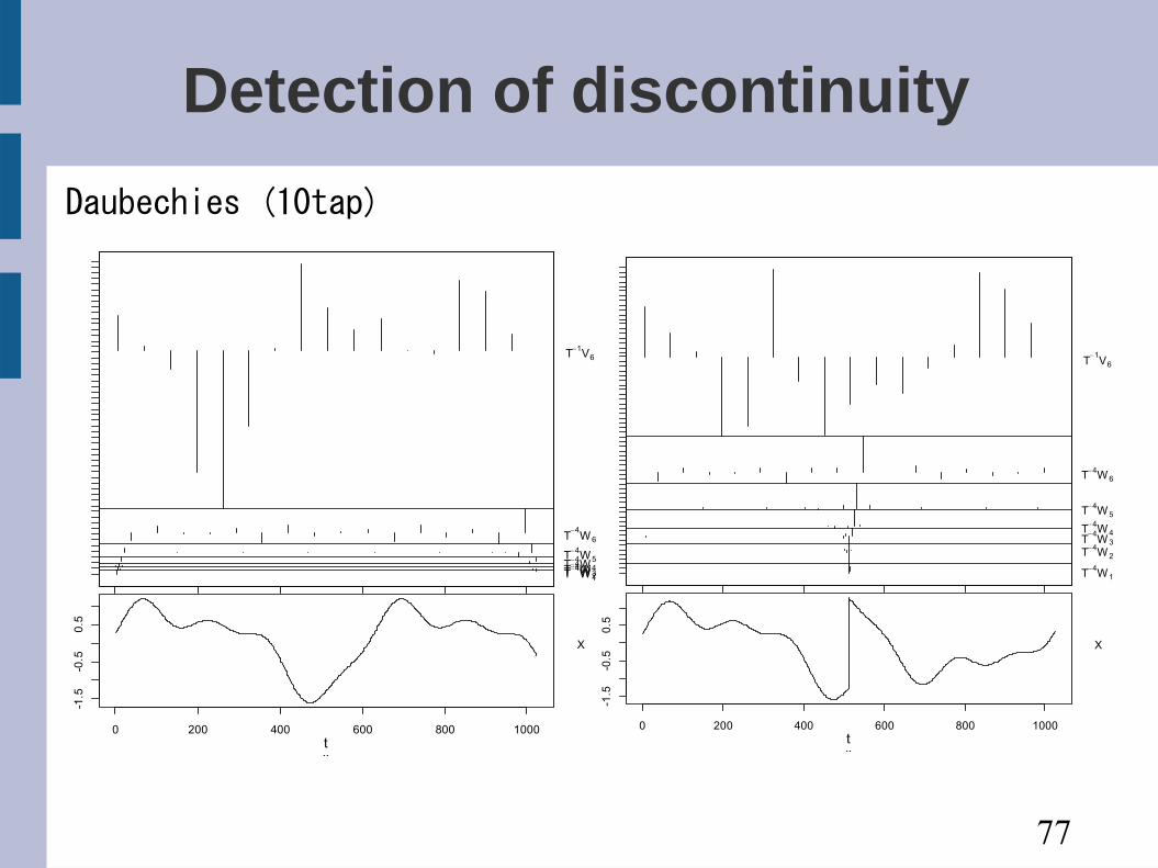
Detection of discontinuity
Daubechies (10tap)
0 200 400 600 800 1000
-1.5
-0.5
0.5
x
X
t
T4
W1T
4W2
T4
W3T4W4
T4W5
T4
W6
T1V6
0 200 400 600 800 1000
-1.5
-0.5
0.5
x
X
t
T4W 1
T4W 2
T4
W 3
T4W 4
T4W 5
T4W 6
T1
V6

78
Detection of discontinuity
Daubechies (20tap)
0 200 400 600 800 1000
-1.5
-0.5
0.5
x
X
t
T8
W1T8W2
T9W3T9W4
T9
W5
T3
V5
0 200 400 600 800 1000
-1.5
-0.5
0.5
x
X
t
T8
W1
T8W2
T9
W3
T9W4
T9
W5
T3
V5
79
0 200 400 600 800 1000
-1.5
-1.0
-0.5
0.0
0.5
1.0
1.5
Index
y
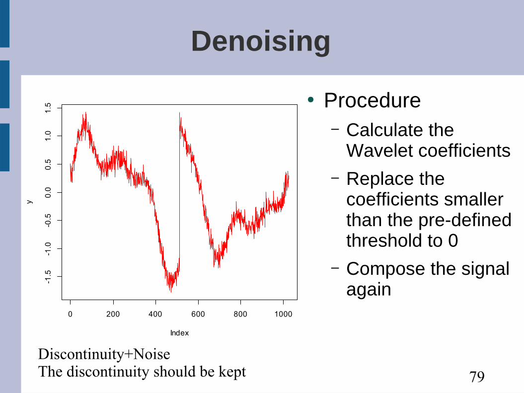
Denoising
● Procedure– Calculate the
Wavelet coefficients– Replace the
coefficients smaller than the pre-defined threshold to 0
– Compose the signal again
Discontinuity+NoiseThe discontinuity should be kept

80
Results
0 200 400 600 800 1000
-1.5
-0.5
0.5
x
X
t
T0
W 1
T0
W 2
T0
W 3T
0W 4
T0
W 5
T0W 6
T0
W 7
T0
W 8
T0
W 9
T0W10T0V10
0 200 400 600 800 1000
-1.5
-0.5
0.5
x
X
t
T0
W 1
T0
W 2
T0
W 3T
0W 4
T0
W 5
T0W 6
T0
W 7
T0
W 8
T0
W 9
T0W10T0V10
Original Haar

81
Results
0 200 400 600 800 1000
-1.5
-0.5
0.5
1.5
x
X
t
T1
W 1
T1W 2T1W 3
T1
W 4
T1
W 5
T1
W 6
T1
W 7
T1W 8
T0
V8
0 200 400 600 800 1000
-1.5
-0.5
0.5
x
X
t
T2
W 1
T2
W 2
T2W 3
T2
W 4
T2W 5
T2
W 6
T2
W 7
T1V7
Daubechies 6tapDaubechies 4tap
82
Results
0 200 400 600 800 1000
-1.5
-0.5
0.5
x
X
t
T8
W 1
T8W 2
T9
W 3
T9
W 4
T9W 5
T3
V5
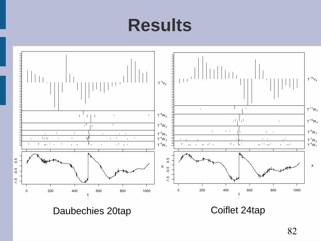
Daubechies 20tap
0 200 400 600 800 1000
-1.5
-0.5
0.5
x
X
t
T4W 1
T7W 2
T9
W 3
T10W4
T11W5
T14
V5
Coiflet 24tap

83
Denoising of speech signal
ORIGINAL NOISY
84
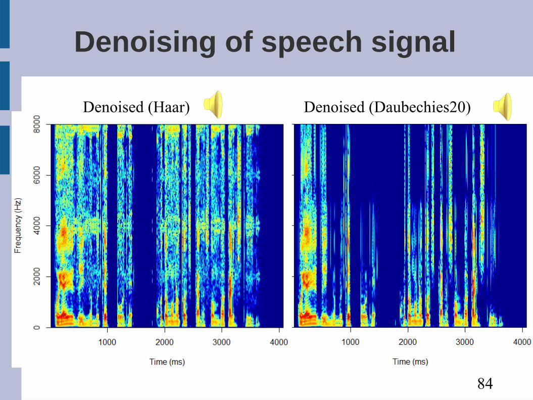
Denoising of speech signal
Denoised (Haar) Denoised (Daubechies20)
85
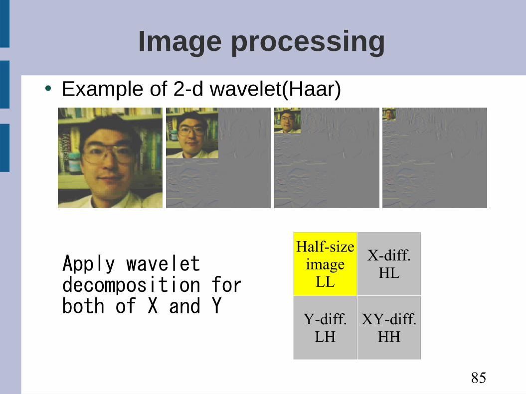
Image processing● Example of 2-d wavelet(Haar)
Apply wavelet decomposition for both of X and Y
Half-sizeimage
LL
X-diff.HL
Y-diff.LH
XY-diff.HH
86
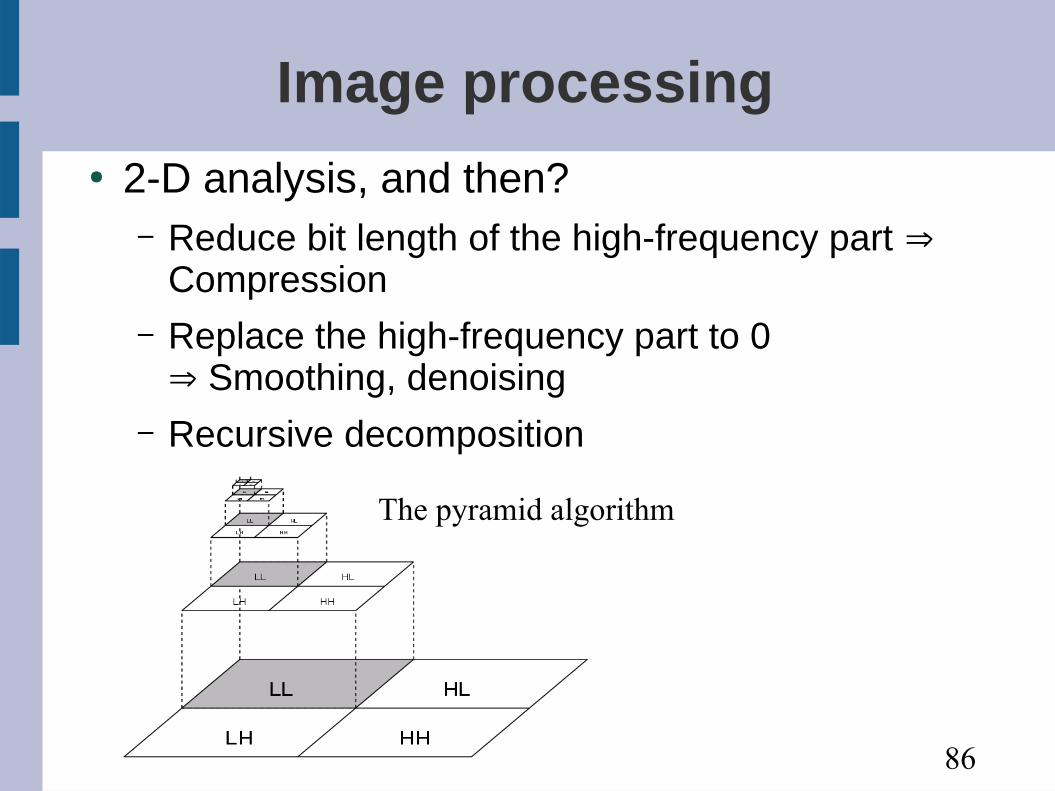
Image processing● 2-D analysis, and then?
– Reduce bit length of the high-frequency part ⇒Compression
– Replace the high-frequency part to 0 Smoothing, denoising⇒
– Recursive decomposition
The pyramid algorithm
87
Image compression● Apply wavelet transform to the image● Quantize the wavelet coefficients
– Coarse quantization of the high-frequency part → Smoothed image
● Entropy (reversible) compression

88
Examples● 256x256 image
Haarwavelet
Truncate the coefficients nearly zero

90
しきい値と画質
Th=10 Th=20

91
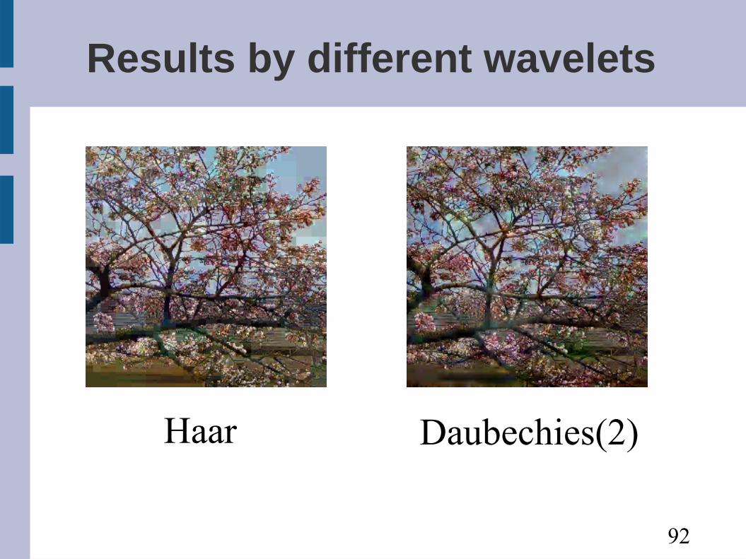
Wavelet and block noise● Why the block noises
appear?– The image is composed by
the superposition of the basis function
– The shape of the basis function (Haar) appears
● Improvement– Use the basis function with
overlapping (such as Daubachies' wavelet)
92
Results by different wavelets
Haar Daubechies(2)

93
The Wavelet Packet● Wavelet transform: split only the low-
frequency part
Original
L H
LL HLH
LLL HLHLLH

94
The Wavelet Packet● Wavelet packet: Split both the lower and
higher parts
Original
L H
LL LH
LLL LLH
HL HH
LHL LHH HLL HLH HHL HHH

95
Best Basis Selection● Choose "how to decompose the signal" by
the Wavelet Packet– Use the evaluation function of "goodness"
● Example: data compression– Make the small-valued coefficients zero– Evaluation function: Number of coefficients
smaller than a threshold

96
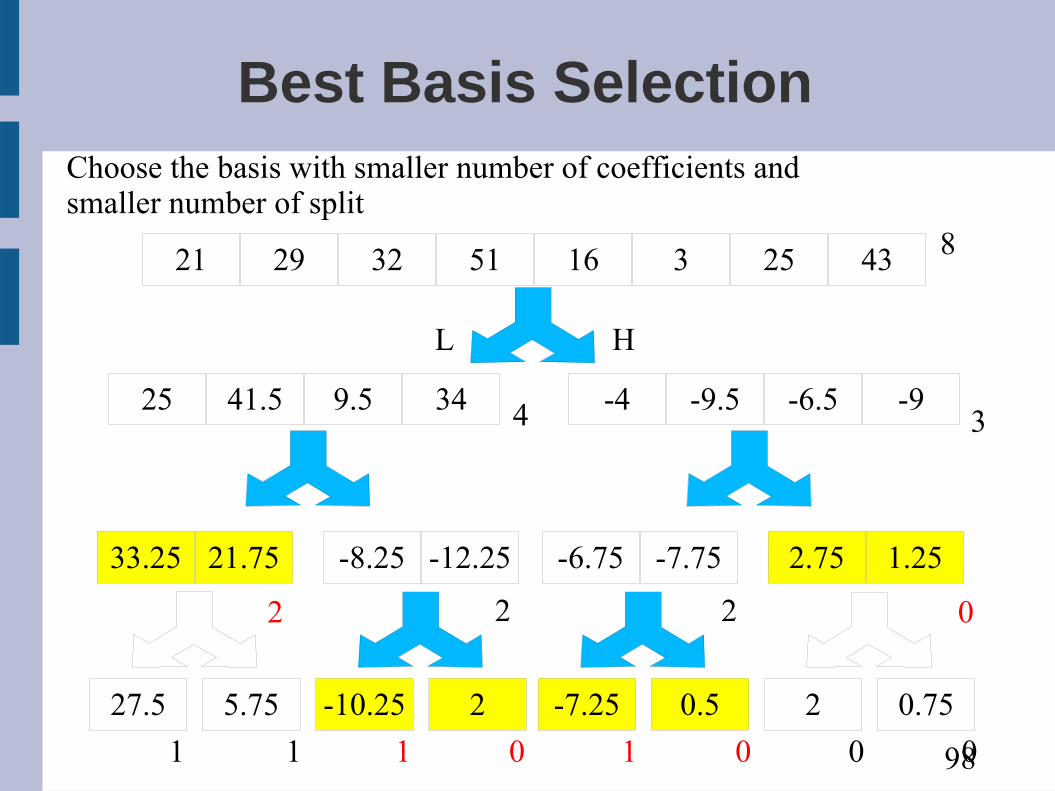
Best Basis Selection
21 29 32 51 16 3 25 43
25 41.5 9.5 34 -4 -9.5 -6.5 -9
33.25 21.75 -8.25 -12.25 -6.75 -7.75 2.75 1.25
27.5 5.75 -10.25 2 -7.25 0.5 2 0.75
L H

97
Best Basis Selection
21 29 32 51 16 3 25 43
25 41.5 9.5 34 -4 -9.5 -6.5 -9
33.25 21.75 -8.25 -12.25 -6.75 -7.75 2.75 1.25
27.5 5.75 -10.25 2 -7.25 0.5 2 0.75
L H
Count the coefficients larger than 5
8
4 3
2 2 2 0
1 1 1 10 0 0 0
98
Best Basis Selection
21 29 32 51 16 3 25 43
25 41.5 9.5 34 -4 -9.5 -6.5 -9
33.25 21.75 -8.25 -12.25 -6.75 -7.75 2.75 1.25
27.5 5.75 -10.25 2 -7.25 0.5 2 0.75
L H
Choose the basis with smaller number of coefficients andsmaller number of split
8
4 3
2 2 2 0
1 1 1 10 0 0 0

99
Note● Wavelet packet is not a simple frequency
analysis
Original signal
12345678High
Low
8765
1234
HH
HL
LH
LL
56
87
12
43
HHH
HHL
HLH
HLL
LHH
LHL
LLH
LLL
6
5
7
8
3
4
2
1


![kakuigaku ref3.ppt [互換モード]chtgkato3.med.hokudai.ac.jp/kougi/kakuigaku_practice/...高速フーリエ変換(FFT : Fast Fourier Transform ) フーリエ変換を高速に計算するアルゴリズム。1942年にDanielson](https://img.pdfslide.tips/doc/110x75/5e2c20610da8373b5c3b99eb/kakuigaku-ref3ppt-fff-eefffifft-fast-fourier.jpg)
![信号処理 - 北海道大学sdm0.5 1 t[] x (t)-d/2 0 d/2 2 sinc /2 sin /2 2 0 2 1 d d d d X d X d t d t x t のフーリエ変換 は フーリエ 変換 振幅スペクトル (d](https://img.pdfslide.tips/doc/110x75/5eda76c8b3745412b5716294/c-oee-05-1-t-x-t-d2-0-d2-2-sinc-2-sin-2-2-0-2.jpg)