AC 00-6A

• • • • • • • • • • • • • .. • • • • • • • • • • • • • • • • • • • • • • • • • • • • • • • • • • • • • • • • • • • • • • • • • • • • • • • • • • • • • • • • • • • • • • • • • • • • • • • • • • • • • • • • • • • • • • • • • • • • • • • • • • • • • • • • • • • • • • • • • • • • • • • • • • • • • • • • • • • • • • • • • • • • • • • • • • • • • • • • • • • • • • • • • • •

AVIATION" WEATH ER

For Pil sand Flight perations Personnel

Revised 1975

DEPARTMENT OF TRANSPORTATION FEDERAL AVIATION ADMINISTRATION FI ight Standards Service

DEPARTMENT OF COMMERCE NATIONAL OCEANIC AND ATMOSPHERIC ADMINISTRATION National Weather Service

Washington, D.C.

Reprinted by asa PUBLICATIONS

AC 00-6A

Editoria 1 Note:

Figures 137 through 139 and 142 on pages 160, 161, and 165 have been rearranged to align with their proper legends. Corresponding corrections have been made in the Contents, page XII.

Editorial Note: (9/82)

Figures 137 through 139 on pages 160 and 161 have been rearranged in order to flow in proper sequence with the text. Corresponding corrections have been made in the Contents, page XII.

For sale by the Superintendent of Documents, U.S. Government Printing Office Washington, D.C. 20402

Preface

AVIATION WEATHER is published jointly by the FAA Flight Standards Service and the National Weather Service (NWS). The publication began in 1943 as CAA Bulletin No. 25, "Meteorology for Pilots," which at the time contained weather knowledge considered essential for most pilots. But as aircraft flew farther, faster, and higher and as meteorological knowledge grew, the bulletin became obsolete. It was revised in 1954 as "Pilots' Weather Handbook" and again in 1965 under its present title.

All these former editions suffered from one common problem. They dealt in part with weather services which change continually in keeping with current tech­niques and service demands. Therefore, each edition became somewhat outdated almost as soon as published; and its obsolescence grew throughout the period it remained in print.

To alleviate this problem, the new authors have completely rewritten this edition streamlining it into a clear, concise, and· readable book and omitting all reference to specific weather services. Thus, the text will remain valid and adequate for many years. A companion manual, AVIATION WEATHER SERVICES, Advisory Circular 00-45, supplements AVIATION WEATHER. This supplement (AC 00-45) periodically is updated to reflect changes brought about by latest techniques, capabilities, and service demands. It explains current weather services and the formats and uses of weather charts and printed weather messages. The two manuals are sold separately; so at a nominal cost, a pilot can purchase a copy of the supplement (AC 00-45) periodically and keep current in aviation weather services.

C. Hugh Snyder, National Weather Service Coordinator and Training Con­sultant at the FAA Academy, directed the preparation of AVIATION WEATHER and AVIATION WEATHER SERVICES. He and his assistant, John W. Zimmerman, Jr., did much of the writing and edited the final manuscripts. Recognition is given to these meteorologists on the NWS Coordinator's staff who helped write the original manu­script, organize the contents, and plan illustrations: Milton Lee Harrison, Edward A. Jessup, Joe L. Kendall, and Richard A. Mitchem. Beatrice Emery deserves special recognition for her relentless effort in typing, retyping, proofing, correcting, and assembling page after page of manuscript. Many other offices and individuals have contributed to the preparation, editing, and publication of the two volumes.

III

Contents

Page

Preface. . . . . . . . . . . . . . . . . . . . . . . . . . . . . . . . . . . . . . . . . . . . . . . . . . . . . . . . . . . . . III Introduction ......................................................... XIII

PART I. WHAT YOU SHOULD KNOW ABOUT WEATHER

CHAPTER 1. THE EARTH'S ATMOSPHERE. . . . . • . . . . . • . . • . . • . . . . . • . . . . . . . . 1 Composition. . . . . . . . . . . . . . . . . . . . . . . . . . . . . . . . . . . . . . . . . . . . . . . . . . . . . 2 Vertical Structure. . . . . . . . . . . . . . . . . . . . . . . . . . . . . . . . . . . . . . . . . . . . . . . . 2 The Standard Atmosphere. . . . . . . . . . . . . . . . . . . . . . . . . . . . . . . . . . . . . . . . . 2 Density and Hypoxia. . . . . . . . . . . . . . . . . . . . . . . . . . . . . . . . . . . . . . . . . . . . . 3

CHAPTER 2. TEMPERATURE........................................... 5 Temperature Scales. . . . . . . . . . . . . . . . . . . . . . . . . . . . . . . . . . . . . . . . . . . . . . 6 Heat and Temperature. . . . . . . . . . . . . . . . . . . . . . . . . . . . . . . . . . . . . . . . . . . 6 Temperature Variations.... . . . . . . . . . . . . . . . . .. . .. . . . . . . . . . . . . . . . . . . 7 In Closing. . . . . . . . . . . . . . . . . . . . . . . . . . . . . . . . . . . . . . . . . . . . . . . . . . . . . . 10

CHAPTER 3. ATMOSPHERIC PRESSURE AND ALTIMETRY. . . . . . . . . . . . . . . . . . . . . 11 Atmospheric Pressure. . . . . . . . . . . . . . . . . . . . . . . . . . . . . . . . . . . . . . . . . . . . . 11 Altimetry. . . . . . . . . . . . . . . . . . . . . . . . . . . . . . . . . . . . . . . . . . . . . . . . . . . . . . . 17 In Closing. . . . . . . . . . . . . . . . . . . . . . . . . . . . . . . . . . . . . . . . . . . . . . . . . . . . . . 21

CHAPTER 4. WIND.................................................. 23 Convection. . . . . . . . . . . . . . . . . . . . . . . . . . . . . . . . . . . . . . . . . . . . . . . . . . . . . . 23 Pressure Gradient Force. . . . . . . . . . . . . . . . . . . . . . . . . . . . . . . . . . . . . . . . . . . 24 Coriolis Force. . . . . . . . . . . . . . . . . . . . . . . . . . . . . . . . . . . . . . . . . . . . . . . . . . . 25 The General Circulation. . . . . . . . . . . . . . . . . . . . . . . . . . . . . . . . . . . . . . . . . . 26 Friction. . . . . . . . . . . . . . . . . . . . . . . . . . . . . . . . . . . . . . . . . . . . . . . . . . . . . . . . . 30 The Jet Stream. . . . . . . . . . . . . . . . . . . . . . . . . . . . . . . . . . . . . . . . . . . . . . . . . . 31 Local and Small Scale Winds. . . . . . . . . . . . . . . . . . . . . . . . . . . . . . . . . . . . . . 31 Wind Shear. . . . . . . . . . . . . . . . . . . . . . . . . . . . . . . . . . . . . . . . . . . . . . . . . . . . . 34 Wind, Pressure Systems, and Weather. . . . . . . . . . . . . . . . . . . . . . . . . . . . . . . 35

CHAPTER 5. MOISTURE, CLOUD FORMATION, AND PRECIPITATION. . . . . . . . . . 37 Water Vapor. . ... .. . ... ... .. . .. . .. . .. . .. . .. . .. . . .. ... ... .. .. . ... 37 Change of State.... . . . . . . . . . . . . . . . . . . . . . . . . . . . . . . . . . . . . . . . . . . . .. . 39 Cloud Formation. . . . . . . . . . . . . . . . . . . . . . . . . . . . . . . . . . . . . . . . . . . . . . . . . 42 Precipitation ................ , . . . . . . . . . . . . . . . . . . . . . . . . . . . . . . . . . . . 42 Land and Water Effects .......................... " . . . . . . . .. . . . . . . 43 In Closing. . . . . . . . . . . . . . . . . . . . . . . . . . . . . . . . . . . . . . . . . . . . . . . . . . . . . . 45

CHAPTER 6. STABLE AND UNSTABLE AIR ..... , ..•.. ,. .•. .. . .. .•.. .• . .•. . 47 Changes Within Upward and Downward Moving Air.... . .. . .. ..... .. 47 Stability and Instability. . . . . . . . . . . . . . . . . . . . . . . . . . . . . . . . . . . . . . . . . . . 49 What Does It All Mean? . . . . . . . . . . . . . . . . .. . .. . .. . . . . . . . . . . . . . .. . . 52

v

Page

CHAPTER 7. CLOUDS. . . . . . . . . . . . . . . . . . . . . . . . . . . . . . . . . . . . . . . . . . . . . . . . . 53 Identification. . . . . . . . . . . . . . . . . . . . . . . . . . . . . . . . . . . . . . . . . . . . . . . . . . . . 53 Signposts in the Sky. . . . . . . . . . . . . . . . . . . . . . . . . . . . . . . . . . . . . . . . . . . . . . 62

CHAPTER 8. Am MASSES AND FRONTS. . . . . . . . . . . . . . . . . . . . . . . . . . . . . . . . . . 63 Air Masses. . . . . . . . . . . . . . . . . . . . . . . . . . . . . . . . . . . . . . . . . . . . . . . . . . . . . . 63 Fronts ............ , .. , .................... , ......... . ..... . .... . 64 Fronts and Flight Planning. . . . . . . . . . . . . . . . . . . . . . . . . . . . . . . . . . . . . . . . 78

CHAPTER 9. TURBULENCE............................................ 79 Convective Currents. . . . . . . . . . . . . . . . . . . . . . . . . . . . . . . . . . . . . . . . . . . . . . 80 Obstructions to Wind Flow. . . . . . . . . . . . . . . . . . . . . . . . . . . . . . . . . . . . . . . . 82 Wind Shear. . . . . . . . . . . . . . . . . . . . . . . . . . . . . . . . . . . . . . . . . . . . . . . . . . . . . 86 Wake Turbulence ... , ..... , .... '" " ................ " . .. .... .... 88 In Closing. . . . . . . . . . . . . . . . . . . . . . . . . . . . . . . . . . . . . . . . . . . . . . . . . . . . . . 90

CHAPTER 10. ICING................................................. 91 Structural Icing. . . . . . . . . . . . . . . . . . . . . . . . . . . . . . . . . . . . . . . . . . . . . . . . . . 92 Induction System Icing. . . . . . . . . . . . . . . . . . . . . . . . . . . . . . . . . . . . . . . . . . . 97 Instrument Icing. . . . . . . . . . . . . . . . . . . . . . . . . . . . . . . . . . . . . . . . . . . . . . . . . 98 Icing and Cloud Types. . . . . . . . . . . . . . . . . . . . . . . . . . . . . . . . . . . . . . . . . . . 99 Other Factors in Icing .......................................... " 100 Ground Icing. . . . . . . . . . . . . . . . . . . . . . . . . . . . . . . . . . . . . . . . . . . . . . . . . . .. 102 Frost .... , ........................... '" ..................... '" 102 In Closing. . . . . . . . . . . . . . . . . . . . . . . . ............................ " 102

CHAPTER 11. THUNDERSTORMS........................................ 105 Where and When? ............................................. " 105 They Don't Just Happen.......................................... 111 The Inside Story ............................................... " 111 Rough and Rougher ............................................ " 112 Hazards. . . . . . . . . . . . . . . . . . . . . . . . . . . . . . . . . . . . . . . . . . . . . . . . . . . . . . . . 113 Thunderstorms and Radar. . . . . . . . . . . . . . . . . . . . . . . . . . . . . . . . . . . . . . .. 120 Do's and Don'ts of Thunderstorm Flying .......................... " 121

CHAPTER 12. COMMON IFR PRODUCERS. . . . . . . . . .. . .. . . . . . . .. . .. . . .... 125 Fog............................................................ 126 Low Stratus Clouds. . . . . . . . . . . . . . . . . . . . . . . . . . . . . . . . . . . . . . . . . . . . .. 128 Haze and Smoke ..... , ...... '" '" ................. , ... , '" .... " 129 Blowing Restrictions to Visibility. . . . . . . . . . . . . . . . . . . . . . . . . . . . . . . . . .. 129 Precipitation .................................................. " 130 Obscured or Partially Obscured Sky .............................. " 130 In Closing. . . . . . . . . . . . . . . . . . . . . . . . . . . . . . . . . . . . . . . . . . . . . ....... " 130

PART II. OVER AND BEYOND

CHAPTER 13. HIGH ALTITUDE WEATHER ............................. " 135 The Tropopause ............................................... " 136 The Jet Stream. . . . . . . . . . . . . . . . . . . . . . . . . . . . . . . . . . . . . . . . . . . . . . . . .. 136 Cirrus Clouds .................................................. " 139 Clear Air Turbulence... . . . . . . . . . . . . . . . . . . . . . . . . . .. . . . . .. . . . . . . . .. 142 Condensation Trails ............................................ " 143

VI

Page

Haze Layers. . . . . . . . . . . . . . . . . . . . . . . . . . . . . . . . . . . . . . . . . . . . . . . . . . . .. 144 Canopy Static. . . . . . . . . . . . . . . . . . . . . . . . . . . . . . . . . . . . . . . . . . . . . . . . . .. 145 Icing ....................... " . .. . . . . . . . . . . . . . . . . . . . . . . .. . . . . . .. 145 Thunderstorms. . . . . . . . . . . . . . . . . . . . . . . . . . . . . . . . . . . . . . . . . . . . . . . . .. 145

CHAPTER 14. ARCTIC WEATHER ••••••..•..•..•••••••..•••......•• " • •. 147 Climate, Air Masses, and Fronts. . . . . . . . . . . . . . . . . . . . . . . . . . . . . . . . . . .. 148 Arctic Peculiarities. . . . . . . . . . . . . . . . . . . . . . . . . . . . . . . . . . . . . . . . . . . . . .. 152 Weather Hazards ................. " ... . .. . ... ... .. ... . .. ... . . ... 153 Arctic Flying Weather. . . . . . . . . . . . . . . . . . . . . . . . . . . . . . . . . . . . . . . . . . .. 154 In Closing. . . . . . . . . . . . . . . . . . . . . . . . . . . . . . . . . . . . . . . . . . . . . . . . . . . . .. 155

CHAPTER 15. TROPICAL WEATHER..... ..• •.•• •• ..•. •.. .•.... ...•. ....• 157 Circulation. . . . . . . . . . . . . . . . . . . . . . . . . . . . . . . . . . . . . . . . . . . . . . . . . . . . .. 158 Transitory Systems. . . . . . . . . . . . . . . . . . . . . . . . . . . . . . . . . . . . . . . . . . . . . .. 162

CHAPTER 16. SOARING WEATHER.... . •• . .• ..•. .. . .• . •• .•• . .• . .•• •.. .•• 171 Thermal Soaring. . . . . . . . . . . . . . . . . . . . . . . . . . . . . . . . . . . . . . . . . . . . . . .. 172 Frontal Soaring. . . . . . . . . . . . . . . . . . . . . . . . . . . . . . . . . . . . . . . . . . . . . . . . .. 191 Sea Breeze Soaring. . . . . . . . . . . . . . . . . . . . . . . . . . . . . . . . . . . . . . . . . . . . . .. 191 Ridge or Hill Soaring.. .. . . . . .. . .. . . . . . . . .. . . . . .. . .. . . . . .. . . . . . . .. 195 Mountain Wave Soaring. . . . . . . . . . . . . . . . . . . . . . . . . . . . . . . . . . . . . . . . .. 198 In Closing. . . . . . . . . . . . . . . . . . . . . . . . . . . . . . . . . . . . . . . . . . . . . . . . . . . . .. 200

Glossary of Weather Terms.. . . . . . . . . . . .. . . . . . . . . . . .. . . . . . . . . . . .. . . . . .. 201

Index. . . . .. ...... ...... ........................ ... ... .......... . ... 215

VII

III ustrations

Figure Page 1. Composition of a dry atmosphere. . . . . . . . . . . . . . . . . . . . . . . . . . . . . . . . . . 2 2. The atmosphere divided into layers based on temperature. . . . . . . . . . . . . 3 3. The two temperature scales in common use. . . . . . . . . . . . . . . . . . . . . . . . . . 6 4. World-wide average surface temperatures in July. . . . . . . . . . . . . . . . . . . . . 8 5. World-wide average surface temperatures in January. . . . . . . . . . . . . . . . . 8 6. Temperature differences create air movement and, at times, cloudiness. . 9 7. Inverted lapse rates or "inversions" . . . . . . . . . . . . . . . . . . . . . . . . . . . . . . . . 10 8. The mercurial barometer. . . . . . . . . . . . . . . . . . . . . . . . . . . . . . . . . . . . . . . . . 12 9. The aneroid barometer. . . . . . . . . . . . . . . . . . . . . . . . . . . . . . . . . . . . . . . . . . . 13

10. The standard atmosphere. . . . . . . . . . . . . . . . . . . . . . . . . . . . . . . . . . . . . . . . . 14 11. Three columns of air showing how decrease of pressure with height varies

with temperature. . . . . . . . . . . . . . . . . . . . . . . . . . . . . . . . . . . . . . . . . . . . . . 15 12. Reduction of station pressure to sea leveL.. . . . . . . . . . . . . . . . . . . . . . . . . . 15 13. Pressure systems. . . . . . . . . . . . . . . . . . . . . . . . . . . . . . . . . . . . . . . . . . . . . . . . . 16 14. Indicated altitude depends on air temperature below the aircraft. . . . . . . 17 15. When flying from high pressure to lower pressure without adjusting your

altimeter, you are losing true altitude.... . . . . . . . . . . . . . . . . . . . . . . . . . 18 16. Effect of temperature on altitude. . . . . . . . . . . . . . . . . . . . . . . . . . . . . . . . . . . 19 17. Effect of density altitude on takeoff and climb. . . . . . . . . . . . . . . . . . . . . . . 20 18. Convective current resulting from uneven heating of air by contrasting

surface temperatures. . . . . . . . . . . . . . . . . . . . . . . . . . . . . . . . . . . . . . . . . . . 24 19. Circulation as it would be on a nonrotating globe. . . . . . . . . . . . . . . . . . . . 25 20. Apparent deflective force due to rotation of a horizontal platform. . . . . . . 26 21. Effect of Coriolis force on wind relative to isobars. . . . . . . . . . . . . . . . . . . . 27 22. In the Northern Hemisphere, Coriolis force turns equatorial winds to

westerlies and polar winds to easterlies. . . . . . . . . . . . . . . . . . . . . . . . . . . . 28 23. Mean world-wide surface pressure distribution in July. . . . . . . . . . . . . . . . 28 24. Mean world-wide surface pressure distribution in January. . . . . . . . . . . . . 29 25. General average circulation in the Northern Hemisphere. . . . . . . . . . . . . . 30 26. Air flow around pressure systems above the friction layer. . . . . . . . . . . . . . 31 27. Surface friction slows the wind and reduces Coriolis force; winds are

deflected across the isobars toward lower pressure. . . . . . . . . . . . . . . . . . 32 28. Circulation around pressure systems at the surface. . . . . . . . . . . . . . . . . . . . 33 29. The "Chinook" is a katabatic (downslope) wind. . . . . . . . . . . . . . . . . . . . . 33 30. Land and sea breezes. . . . . . . . . . . . . . . . . . . . . . . . . . . . . . . . . . . . . . . . . . . . 34 31. Wind shear. . . . . . . . . . . . . . . . . . . . . . . . . . . . . . . . . . . . . . . . . . . . . . . . . . . . . 35 32. Blue dots illustrate the increased water vapor capacity of warm air. . . . . 38 33. Relative humidity depends on both temperature and water vapor. . . . . . 39 34. Virga. . . . . . . . . . . . . . . . . . . . . . . . . . . . . . . . . . . . . . . . . . . . . . . . . . . . . . . . . . 40 35. Heat transactions when water changes state. . . . . . . . . . . . . . . . . . . . . . . . . 41 36. Growth of raindrops by collision of cloud droplets. . . . . . . . . . . . . . . . . . . . 42 37. Lake effects ...................................... , ........... , . . 43 38. Strong cold winds across the Great Lakes absorb water vapor and may

carry showers as far eastward as the Appalachians. . . . . . . . . . . . . . . . . . 44 39. A view of clouds from 27,000 feet over Lake Okeechobee in southern

Florida ............... , . . . . .. . .. . ..... . ..... . .. . .. . .. . ..... . .. 45

IX

Figure Page 40. Decreasing atmospheric pressure causes the balloon to expand as it rises 48 41. Adiabatic warming of downward moving air produces the warm Chinook

wind......................................................... 49 42. Stability related to temperatures aloft and adiabatic cooling. . . . . . . . . . . 50 43. When stable air is forced upward, cloudiness is flat and stratified. When

unstable air is forced upward, cloudiness shows extensive vertical development. . . . . . . . . . . . . . . . . . . . . . . . . . . . . . . . . . . . . . . . . . . . . . . . . . 51

44. Cloud base determination. . . . . . . . . . . . . . . . . . . . . . . . . . . . . . . . . . . . . . . . . 52 45. Cirrus..... . . . . . . . . . . . . . . . . . . . . . . . . . . . . . . . . . . . . . . . . . . . . . . . . . . . . . 54 46. Cirrocumulus. . . . . . . . . . . . . . . . . . . . . . . . . . . . . . . . . . . . . . . . . . . . . . . . . . . 55 47. Cirrostratus............................................. .. . .. . . . 55 48. Altocumulus. . . . . . . . . . . . . . . . . . . . . . . . . . . . . . . . . . . . . . . . . . . . . . . . . . . . 56 49. Altostratus.... . .. . .. . . . . . . . . . . . . . . . . . . . . . . . . . . . . . . . . . . . . . . . . .. . . 56 50. Altocumulus castella nus . . . . . . . . . . . . . . . . . . . . . . . . . . . . . . . . . . . . . . . . . . 57 51. Standing lenticular altocumulus clouds. . . . . . . . . . . . . . . . . . . . . . . . . . . . . 58 52. Nimbostratus. . . . . . . . . . . . . . . . . . . . . . . . . . . . . . . . . . . . . . . . . . . . . . . . . . . 59 53. Stratus.. . . . . . . . . . . . . . . . . . . . . . . . . . . . . . . . . . . . . . . . . . . . . . . . . . . . . . . . 59 54. Stratocumulus..... . . . . . . . . . . . . . . . . . . . . . . . . . . . . . . . . . . . . . . . . . . . . . . 60 55. Cumulus. . . . . . . . . . . . . . . . . . . . . . . . . . . . . . . . . . . . . . . . . . . . . . . . . . . . . . . 60 56. Towering cumulus.. . . . . . . . . . . . . . . . . . . . .. . . . . . . . . . . .. . . . . . . . . . . . . 61 57. Cumulonimbus ........ , ................ '" '" ............. " .. . . 61 58. Horizontal uniformity of an air mass. . . . . . . . . . . . . . . . . . . . . . . . . . . . . . . 64 59. Cross section of a cold front with the weather map symbol. . . . . . . . . . . . . 66 60. Cross section of a warm front with the weather map symbol. . . . . . . . . . . 67 61. Cross section of a stationary front and its weather map symbol. . . . . . . . . 68 62. The life cycle of a frontal wave. . . . . . . . . . . . . . . . . . . . . . . . . . . . . . . . . . . . 69 63. Cross section of a warm-front occlusion and its weather map symbol. . . . 70 64. Cross section of a cold-front occlusion. . . . . . . . . . . . . . . . . . . . . . . . . . . . . . 71 65. Frontolysis of a stationary front. . . . . . . . . . . . . . . . . . . . . . . . . . . . . . . . . . . . 71 66. Frontogenesis of a stationary front. . . . . . . . . . . . . . . . . . . . . . . . . . . . . . . . . . 72 67. A cold front underrunning warm, moist, stable air. . . . . . . . . . . . . . . . . . . . 73 68. A cold front underrunning warm, moist, unstable air. . . . . . . . . . . . . . . . . 73 69. A warm front with overrunning moist, stable air. . . . . . . . . . . . . . . . . . . . . 74 70. A slow-moving cold front underrunning warm, moist, unstable air. . . . . . 74 71. A warm front with overrunning warm, moist, unstable air. . . . . . . . . . . . . 75 72. A fast moving cold front underrunning warm, moist, unstable air... . . . . 75 73. A warm front occlusion lifting warm, moist, unstable air. . . . . . . . . . . . . . 76 74. A cold front occlusion lifting warm, moist, stable air. . . . . . . . . . . . . . . . . . 76 75. An aerial view of a portion of a squall line. . . . . . . . . . . . . . . . . . . . . . . . . . 77 76. Effect of convective currents on final approach. . . . . . . . . . . . . . . . . . . . . . . 80 77. Avoiding turbulence by flying above convective clouds.. . . . . . . . . . . . . . . 81 78. Eddy currents formed by winds blowing over uneven ground or over

obstructions. . . . . . . . . . . . . . . . . . . . . . . . . . . . . . . . . . . . . . . . . . . . . . . . . . . 82 79. Turbulent air in the landing area. . . . . . . . . . . . . . . . . . . . . . . . . . . . . . . . . . 83 80. Wind flow in mountain areas... . . . . . . . . . . . . . . . . . . . . . . . . . . . . . . . . . . . 84 81. Schematic cross section of a mountain wave. . . . . . . . . . . . . . . . . . . . . . . . . 84 82. Standing lenticular clouds associated with a mountain wave. . . . . . . . . . . 85 83. Standing wave rotor clouds marking the rotary circulation beneath

mountain waves .......................................... , . . . . 86 84. Mountain wave clouds over the Tibetan Plateau photographed from a

manned spacecraft. . . . . . . . . . . . . . . . . . . . . . . . . . . . . . . . . . . . . . . . . . . . . 87

x

Figure Page 85. Satellite photograph of a mountain wave and the surface analysis for

approximately the same time. . . . . . . . . . . . . . . . . . . . . . . . . . . . . . . . . . . . 87 86. Wind shear in a zone between relatively calm wind below an inversion and

strong wind above the inversion. . . . . . . . . . . . . . . . . . . . . . . . . . . . . . . . . 88 87. Wake turbulence wing tip vortices developing as aircraft breaks ground. 89 88. Planning landing or takeoff to avoid heavy aircraft wake turbulence. . . . 90 89. Effects of structural icing. . . . . . . . . . . . . . . . . . . . . . . . . . . . . . . . . . . . . . . . . 92 90. Clear, rime, and mixed icing on airfoils.. . . . . .. . . . . . . . . . . . . . .. . . . . . . 93 91. Clear wing icing (leading edge and underside). . . . . . . . . . . . . . . . . . . . . . . 94 92. Propeller icing. . . . . . . . . . . . . . . . . . . . . . . . . . . . . . . . . . . . . . . . . . . . . . . . . . 95 93. Rime icing on the nose of a Mooney "Mark 21" aircraft. . . .. . . . . . . .. . 96 94. External icing on a pitot tube. . . . . . . . . . . . . . . . . . . . . . . . . . . . . . . . . . . . . 97 95. Carburetor icing. . . . . . . . . . . . . . . . . . . . . . . . . . . . . . . . . . . . . . . . . . . . . . . . . 98 96. Internal pitot tube icing. . . . . . . . . . . . . . . . . . . . . . . . . . . . . . . . . . . . . . . . . . 99 97. Clear ice on an aircraft antenna mast. . . . . . . . . . . . . . . . . . . . . . . . . . . . . .. 100 98. Freezing rain with a warm front and a cold front. . . . . . .. . . . . . . . . . . .. 101 99. Frost on an aircraft. . . . . . . . . . . . . . . . . . . . . . . . . . . . . . . . . . . . . . . . . . . . .. 103

100. The average number of thunderstorms each year. . . . . . . . . . . . . . . . . . . .. 106 101. The average number of days with thunderstorms during spring. . . . . . . .. 107 102. The average number of days with thunderstorms during summer. . . . . .. 108 103. The average number of days with thunderstorms during fall. . . . . . . . . .. 109 104. The average number of days with thunderstorms during winter. . . . . . .. 110 105. The stages of a thunderstorm... . .. . . . . .. . . . . .. . .. . . . . . . . . . . . . . .. .. 112 106. Schematic of the mature stage of a steady state thunderstorm cell ..... " 113 107. A tornado. . . .. . .. ......... . ... ... .. ....... .. ... . .. . ........ .... 114 108. A waterspout. . . . . . .. . ..... . ......... .. .......... ........... .... 114 109. Funnel clouds. . . . . . . . . . . . . . . . . . . . . . . . . . . . . . . . . . . . . . . . . . . . . . . . . .. 115 110. Cumulonimbus Mamma clouds.................................... 116 111. Tornado incidence by State and area. . . . . . . . . . . . . . . . . . . . . . . . . . . . . .. 117 112. Squall line thunderstorms.. . . . . . . . . . . . . . . . . . . . . . . . . . . . . . . . . . . . . . .. 118 113. Schematic cross section of a thunderstorm.. . . . . . . . .. . .. . .. . .. . . . . . .. 119 114. Hail damage to an aircraft... . . . . . . . . . . . . . . . . . . . . . . .. . .. . .. . . . . . .. 120 115. Radalphotograph of a line of thunderstorms ....... '. . . . . . . . . . . . . . . .. 121 116. Use of airborne radar to avoid heavy precipitation and turbulence. . . . .. 122 117. Ground fog as seen from the air ................................. " 126 118. Advection fog in California. . . . . . . . . . . . . . . . . . . . . . . . . . . . . . . . . . . . . .. 127 119. Advection fog over the southeastern United States and Gulf Coast. . . . .. 128 120. Smoke trapped in stagnant air under an inversion. . . . . . . . . . . . . . . . . . .. 129 121. Aerial photograph of blowing dust approaching with a cold front. . . . . .. 130 122. Difference between the ceiling caused by a surface-based obscuration and

the ceiling caused by a layer aloft. . . . . . . . . . . . . . . . . . . . . . . . . . . . . . .. 131 123. A cross section of the upper troposphere and lower stratosphere. . . . . . .. 136 124. Artist's concept of the jet stream. . . . . . . . . . . . . . . . . . . . . . . . . . . . . . . . . .. 137 125. Ajet stream segment... . .. . . . . ......... ....................... ... 137 126. Multiple jet streams. . . . . . . . . . . . . . . . . . . . . . . . . . . . . . . . . . . . . . . . . . . . .. 138 127. Mean jet positions relative to surface systems. . . . . . . . . . . . . . . . . . . . . . .. 139 128a. Satellite photograph of an occluded system. . .. . . . . . . . . . . . . . . . . . . . . . 140 128b. Infrared photograph of the system shown in figure 128a.. . . . . . . . . . . .. 141 129. A frequent CAT location is along the jet stream north and northeast of a

rapidly deepening surface low. . . . . . . . . . . . . . . . . . . . . . . . . . . . . . . . . .. 142 130. Contrails....................................................... 144

XI

Figure Page 131. The Arctic... .. . . . . . . . . . . . . . . . . . . . . . . . . . . . . . . . . . . . . . . . . . . . . . . . .. 148 132. Sunshine in the Northern Hemisphere .................. " . .. . . . . . .. 149 133. The permanent Arctic ice pack ............... , . . . . .. . . . . . . . . . . . . .. 150 134. Average number of cloudy days per month (Arctic) ................. , 151 135. Visibility reduced by blowing snow. . . . . . . . . . . . . . . . . . . . . . . . . . . . . . . .. 154 136. A typical frozen landscape of the Arctic.. .. . . . . . . . . . . . . . . . . . . . . . . . .. 154 137. Vertical cross section illustrating convection in the Intertropical 'Con-

vergence Zone. . . . . . . . . . . . . . . . . . . . . . . . . . . . . . . . . . . . . . . . . . . . . . .. 160 138. Prevailing winds throughout the Tropics in July. . . . . . . . . . . . . . . . . . . .. 161 139. Prevailing winds in the Tropics in January. . . . . . . . . . . . . . . . . . . . . . . . .. 161 140. A shear line and an induced trough caused by a polar high pushing into

the subtropics .................... " . .. . . . . . . . . . . . . . .. . . . . . . . .. 163 141. A trough aloft across the Hawaiian Islands. . . . . . . . . . . . . . . . . . . . . . . . .. 164 142. A Northern Hemisphere easterly wave ......... " . . . . . . . . . . . . . . . . . .. 165 143. Vertical cross section along line A-B in figure 142.. . .. . .. . .. . .. . .... 165 144. Principal regions where tropical cyclones form and their favored direc-

tions of movement. . . . . . . . . . . . . . . . . . . . . . . . . . . . . . . . . . . . . . . . . . . .. 166 145. Radar photograph of hurricane "Donna". . . .. . .. . . . . . . . . . . .. . . . . . .. 168 146. A hurricane observed by satellite. . .. . . . . . . . . . . . . . . . . . . . . . . . . . . . . . .. 169 147. Thermals generally occur over a small portion of an area while down-

drafts predominate. . . . . . . . . . . . . . . . . . . . . . . . . . . . . . . . . . . . . . . . . . . .. 172 148. Using surface dust and smoke movement as indications of a thermal. . .. 174 149. Horizontal cross section of a dust devil rotating clockwise ..... '" .. . ... 174 150. Cumulus clouds grow only with active thermals.. . .. . . . . . . . . . . . . . . . .. 176 151. Photograph of a dying cumulus... . .. .... .. .... .. . .. ...... . .. . . . ... 177 152. Altocumulus castellanus clouds are middle level convective clouds. . . . .. 178 153. Experience indicates that the "chimney" thermal is the most prevalent

type ........ , . . . . .. . .. . . . . .. . . . . . . . . . . . . . .. . . . . . . . .. . . . . . . . .. 179 154. Thermals may be intermittent "bubbles" ............... " . . . . . . . . .. 179 155. It is believed that a bubble thermal sometimes develops a vortex ring. .. 180 156. Wind causes thermals to lean. . . . . . . . . . . . . . . . . . . . . . . . . . . . . . . . . . . . .. 181 157. Photograph of cumulus clouds severed by wind shear. . . . . . . . . . . . . . . .. 181 158. Conditions favorable for thermal streeting. . . . . . . . . . . . . . . . . . . . . . . . . .. 182 159. Cumulus clouds in thermal streets photographed from a satellite high

resolution camera.... . . . . . . . .. . . . . . . . . . . . . . . . . . . . . . . . . . .. . .. . .. 183 160. The Pseudo-Adiabatic Ohart. . . . . . . . . . . . . . . . . . . . . . . . . . . . . . . . . . . . .. 184 161. An early morning upper air observation plotted on the pseudo-adiabatic

chart ................................... '" .......... " . .. ... 185 162. Computing the thermal index (TI).... . . . . . . . . . . . . . . . . . . . . . . . . . . . .. 187 163. Another example of computing TI's and maximum height of thermals... 188 l64. An upper air observation made from an aircraft called an airplane

observation or APOB. . . . . . . . . . . . . . . . . . . . . . . . . . . . . . . . . . . . . . . . .. 189 165. Schematic cross section through a sea breeze front. . . . . . . . . . . . . . . . . . .. 192 166. Sea breeze flow into the San Fernando Valley ....... " ............. , 193 167. Sea breeze convergence zone, Cape Cod, Massachusetts. . . . . . . . . . . . . .. 194 168. Schematic cross section of airflow over a ridge. ...................... 195 169. Strong winds flowing around an isolated peak. . . . . . . . . . . . . . . . . . . . . .. 196 170. Wind flow over various types of terrain. . . . . . . . . . . . . . . . . . . . . . . . . . . .. 197 171. Schematic cross section of a mountain wave. . . . . . . . . . . . . . . . . . . . . . . .. 198 172. Wave length and amplitude... . .. . . . . ..... . . . . . . . . . . . . . . . . . . . . .. .. 199

XII

Introduction

Weather is perpetual in the state of the atmosphere. All flying takes place in the atmosphere, so flying and weather are inseparable. Therefore, we cannot treat aviation weather purely as an academic subject. Throughout the book, we discuss each aspect of weather as it relates to aircraft operation and flight safety. However, this book is in no wayan aircraft operating manual. Each pilot must apply the knowledge gained here to his own aircraft and flight capabilities.

The authors have devoted much of the book to marginal, hazardous, and violent weather which becomes a vital concern. Do not let this disproportionate time devoted to hazardous weather discourage you from flying. By and large, weather is generally good and places little restriction on flying. Less frequently, it becomes a threat to the VFR pilot but is good for IFR flight. On some occasions it becomes too violent even for the IFR pilot.

It behooves every pilot to learn to appreciate good weather, to recognize and respect marginal or hazardous weather, and to avoid violent weather when the atmo­sphere is on its most cantankerous behavior. For your safety and the safety of those with you, learn to recognize potential trouble and make sound flight decisions before it is too late. This is the real purpose of this manual.

AVIATION WEATHER is in two parts. Part I explains weather facts every piiot should know. Part II contains topics of special interest discussing high altitude, Arctic, tropical, and soaring weather. A glossary defines terms for your reference while reading this or other weather writings. To get a complete operational study, you will need in addition to this manual a copy of AVIATION WEATHER SERVICES, AC 00-45, which is explained in the Preface.

We sincerely believe you will enjoy this book and at the same time increase your flying safety and economy and, above all, enhance the pleasure and satisfaction of using today's most modem transportation.

XIII

o

Part ONE

WHAT YOU SHOULD KNOW

ABOUT WEATHER

Chapter 1 HE EARTH'S ATMOSPHERE

Planet Earth is unique in that its atmosphere sustains life as we know it. Weather-the state of the atmosphere-at any given time and place strongly influences our daily routine as well as our general life patterns. Virtually all of our activities are affected by weather, but of all man's endeav­ors, none is influenced more intimately by weather than aviation.

Weather is complex and at times difficult to un­derstand. Our restless atmosphere is almost con-

stantly in motion as it strives to reach equilibrium. These never-ending air movements set up chain reactions which culminate in a continuing variety of weather. Later chapters in this book delve into the atmosphere in motion. This chapter looks brief­ly at our atmosphere in terms of its composition; vertical structure; the standard atmosphere; and of special concern to you, the pilot, density and hypoxia.

COMPOSITION

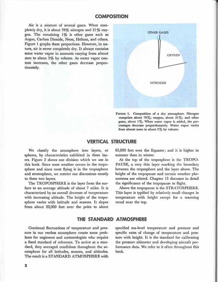
Air is a mixture of several gases. When com­pletely dry, it is about 78% nitrogen and 21 % oxy­gen. The remaining 1 % is other gases such as Argon, Carbon Dioxide, Neon, Helium, and others. Figure 1 graphs these proportions. However, in na­ture, air is never completely dry. It always contains some water vapor in amounts varying from almost zero to about 5% by volume. As water vapor con­tent increases, the other gases decrease propor­tionately.

OTHER GASES

.1/

OXYGEN

NITROGEN

FIGURE 1. Composition of a dry atmosphere. Nitrogen comprises about 78%; oxygen, about 21 %; and other gases, about 1 %. When water vapor is added, the per­centages decrease proportionately. Water vapor varies from almost none to about 5% by volume.

VERTICAL STRUCTURE

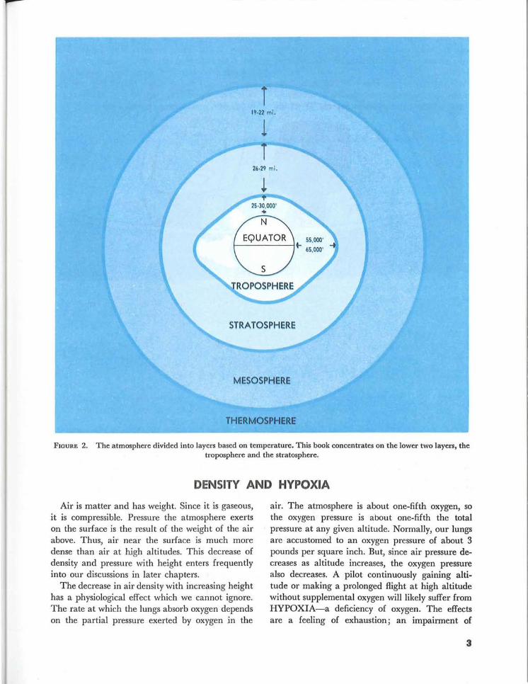
We classify the atmosphere into layers, or spheres, by characteristics exhibited in these lay­ers. Figure 2 shows one division which we use in this book. Since most weather occurs in the tropo­sphere and since most flying is in the troposphere and stratosphere, we restrict our discussions mostly to these two layers.

The TROPOSPHERE is the layer from the sur­face to an average altitude of about 7 miles. It is characterized by an overall decrease of temperature with increasing altitude. The height of the tropo­sphere varies with latitude and seasons. It slopes from about 20,000 feet over the poles to about

65,000 feet over the Equator; and it is higher in summer than in winter.

At the top of the troposphere is the TROPO­PAUSE, a very thin layer marking the boundary between the troposphere and the layer above. The height of the tropopause and certain weather phe­nomena are related. Chapter 13 discusses in detail the significance of the tropopause to flight.

Above the tropopause is the STRATOSPHERE. This layer is typified by relatively small changes in temperature with height except for ' a warming trend near the top.

THE STANDARD ATMOSPHERE

Continual fluctuations of temperature and pres­sure in our restless atmosphere create some prob­lems for engineers and meteorologists who require a fixed standard of reference. To arrive at a stan­dard, they averaged conditions throughout the at­mosphere for all latitudes, seasons, and altitudes. The result is a STANDARD ATMOSPHERE with

2

specified sea-level temperature and pressure and specific rates of change of temperature and pres­sure with height. It is the standard for calibrating the pressure altimeter and developing aircraft per­formance data. We refer to it often throughout this book.

T 19-22 mi.

STRA TOSPHERE

MESOSPHERE

THERMOSPHERE

FIGURE 2. The atmosphere divided into layers based on temperature. This book concentrates on the lower two layers, the troposphere and the stratosphere.

DENSITY AND HYPOXIA

Air is matter and has weight. Since it is gaseous, it is compressible. Pressure the atmosphere exerts on the surface is the result of the weight of the air above. Thus, air near the surface is much more dense than air at high altitudes. This decrease of density and pressure with height enters frequently into our discussions in later chapters.

The decrease in air density with increasing height has a physiological effect which we cannot ignore. The rate at which the lungs absorb oxygen depends on the partial pressure exerted by oxygen in the

air. The atmosphere is about one-fifth oxygen, so the oxygen pressure is about one-fifth the total pressure at any given altitude. Normally, our lungs are accustomed to an oxygen pressure of about 3 pounds per square inch. But, since air pressure de­creases as altitude increases, the oxygen pressure also decreases. A pilot continuously gaining alti­tude or making a prolonged flight at high altitude without supplemental oxygen will likely suffer from HYPOXIA-a deficiency of oxygen. The effects are a feeling of exhaustion; an impairment of

3

vision and judgment; and finally, unconsciousness. Cases are known where a person lapsed into un­consciousness without realizing he was suffering the effects.

When flying at or above 10,000 feet, force yourself to remain alert. Any feeling of drowsiness or undue fatigue may be from hypoxia. If you do

4

not have oxygen, descend to a lower altitude. If fatigue or drowsiness continues after descent, it is caused by something other than hypoxia.

A safe procedure is to use auxiliary oxygen dur­ing prolonged flights above 10,000 feet and for even short flights above 12,000 feet. Above about 40,000 feet, pressurization becomes essential.

Chapter 2 TEMPERATURE

Since early childhood, you have expressed the comfort of weather in degrees of temperature. Why, then, do we stress temperature in aviation weather? Look at your flight computer; tempera­ture enters into the computation of most param­eters on the computer. In fact, temperature can

be critical to some flight operations. As a founda­tion for the study of temperature effects on avia­tion and weather, this chapter describes commonly used temperature scales, relates heat and tempera­ture, and surveys temperature variations both at the surface and aloft.

5

TEMPERATURE SCALES

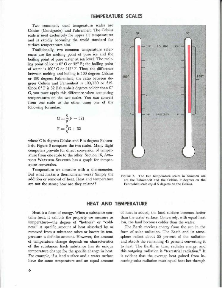
Two commonly used temperature scales are Celsius (Centigrade) and Fahrenheit. The Celsius scale is used exclusively for upper air temperatures and is rapidly becoming the world standard for surface temperatures also.

Traditionally, two common temperature refer­ences are the melting point of pure ice and the boiling point of pure water at sea level. The melt­ing point of ice is 0° C or 32° F; the boiling point of water is 100° C or 212° F. Thus, the difference between melting and boiling is 100 degrees Celsius or 180 degrees Fahrenheit; the ratio between de­grees Celsius and Fahrenheit is 100/180 or 5/9. Since 0° F is 32 Fahrenheit degrees colder than 0° C, you must apply this difference when comparing temperatures on the two scales. You can convert from one scale to the other using one of the following formulae:

5 C = 9(F - 32)

F = 2c + 32 5

where C is degrees Celsius and F is degrees Fahren­heit. Figure 3 compares the two scales. Many flight computers provide for direct conversion of temper­ature from one scale to the other. Section 16, AVIA­TION WEATHER SERVICES has a graph for temper­ature conversion.

Temperatllre we measure with a thermometer. But what makes a thermometer work? Simply the addition or removal of heat. Heat and temperature are not the same; how are they related?

FIGURE 3. The two temperature scales in common use are the Fahrenheit and the Celsius. 9 degrees on the Fahrenheit scale equalS degrees on the Celsius.

HEAT AND TEMPERATURE

Heat is a form of energy. When a substance con­tains heat, it exhibits the property we measure as temperature-the degree of "hotness" or "cold­ness." A specific amount of heat absorbed by or removed from a substance raises or lowers its tem­perature a definite amount. However, the amount of temperature change depends on characteristics of the substance. Each substance has its unique temperature change for the specific change in heat. For example, if a land surface and a water surface have the same temperature and an equal amount

6

of heat is added, the land surface becomes hotter than the water surface. Conversely, with equal heat loss, the land becomes colder than the water.

The Earth receives energy from the sun in the form of solar radiation. The Earth and its atmo­sphere reflect about 55 percent of the radiation and absorb the remaining 45 percent converting it to heat. The Earth, in turn, radiates energy, and this outgoing radiation is "terrestrial radiation." It is evident that the average heat gained from in­coming solar radiation must equal heat lost through

terrestrial radiation in order to keep the earth from getting progressively hotter or colder. How­ever, this balance is world-wide; we must consider

regional and local imbalances which create temper­ature variations.

TEMPERATURE VARIATIONS

The amount of solar energy received by any re­gion varies with time of day, with seasons, and with latitude. These differences in solar energy create temperature variations. Temperatures also vary with differences in topographical surface and with altitude. These temperature variations create forces that drive the atmosphere in its endless motions.

DIURNAL VARIATION Diurnal variation is the change in temperature

from day to night brought about by the daily rota­tion of the Earth. The Earth receives heat during the day by solar radiation but continually loses heat by terrestrial radiation.Warming and cooling depend on an imbalance of solar and terrestrial radiation. During the day, solar radiation exceeds terrestrial radiation and the surface becomes warmer. At night, solar radiation ceases, but ter­restrial radiation continues and cools the surface. Cooling continues after sunrise until solar radiation again exceeds terrestrial radiation. Minimum tem­perature usually occurs after sunrise, sometimes as much as one hour after. The continued cooling after sunrise is one reason that fog sometimes forms shortly after the sun is above the horizon. We will have more to say about diurnal variation and topo­graphic surfaces.

SEASONAL VARIATION In addition to its daily rotation, the Earth re­

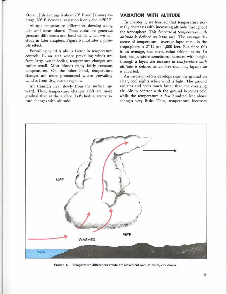
volves in a complete orbit around the sun once each year. Since the axis of the Earth tilts to the plane of orbit, the angle of incident solar radiation varies seasonally between hemispheres. The Northern Hemisphere is warmer in June, July, and August because it receives more solar energy than does the Southern Hemisphere. During December, January, and February, the opposite is true; the Southern Hemisphere receives more solar energy and is warmer. Figures 4 and 5 show these seasonal sur­face temperature variations.

VARIATION WITH LATITUDE The shape of the Earth causes a geographical

variation in the angle of incident solar radiation.

Since the Earth is essentially spherical, the sun is more nearly overhead in equatorial regions than at higher latitudes. Equatorial regions, therefore, re­ceive the most radiant energy and are warmest. Slanting rays of the sun at higher latitudes deliver less energy over a given area with the least being received at the poles. Thus, temperature varies with latitude from the warm Equator to the cold poles. You can see this average temperature gradient in figures 4 and 5.

VARIATIONS WITH TOPOGRAPHY Not related to movement or shape of the earth

are temperature variations induced by water and terrain. As stated earlier, water absorbs and radi­ates energy with less temperature change than does land. Large, deep water bodies tend to minimize temperature changes, while continents favor large changes. Wet soil such as in swamps and marshes is almost as effective as water in suppressing tem­perature changes. Thick vegetation tends to control temperature changes since it contains some water and also insulates against heat transfer between the ground and the atmosphere. Arid, barren surfaces permit the greatest temperature changes.

These topographical influences are both diurnal and seasonal. For example, the difference between a daily maximum and minimum may be 10° or less over water, near a shore line, or over a swamp or marsh, while a difference of 50° or more is common over rocky or sandy deserts. Figures 4 and 5 show the seasonal topographical variation. Note that in the Northern Hemisphere in July, temperatures are warmer over continents than over oceans; in January they are colder over continents than over oceans. The opposite is true in the South­ern Hemisphere, but not as pronounced because of more water surface in the Southern Hemisphere.

To compare land and water effect on seasonal temperature variation, look at northern Asia and at southern California near San Diego. In the deep continental interior of northern Asia, July average temperature is about 50° F; and January average, about -30° F. Seasonal range is about 80° F. Near San Diego, due to the proximity of the Pacific

7

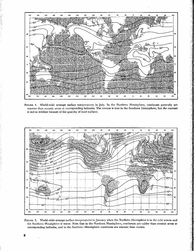
FIGURE 4. World-wide average surface temperatures in July. In the Northern Hemisphere, continents generally are warmer than oceanic areas at corresponding latitudes. The reverse is true in the Southern Hemisphere, but the contrast is not so evident because of the sparcity of land surfaces.

100 120 140 160 180 160 140 120 "'0 60 60 40 20 20 40 60 60 100

FIGURE 5. World-wide average surface temperatures in January when the Northern Hemisphere is in the cold season and the Southern Hemisphere is warm. Note that in the Northern Hemisphere, continents are colder than oceanic areas at corresponding latitudes, and in the Southern Hemisphere continents are warmer than oceans.

8

Ocean, July average is about 70° F and January av­erage, 50° F. Seasonal variation is only about 20° F.

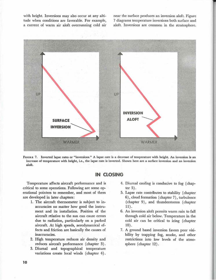
Abrupt temperature differences develop along lake and ocean shores. These variations generate pressure differences and local winds which we will study in later chapters. Figure 6 illustrates a possi­ble effect.

Prevailing wind is also a factor in temperature controls. In an area where prevailing winds are from large water bodies, temperature changes are rather small. Most islands enjoy fairly constant temperatures. On the other hand, temperature changes are more pronounced where prevailing wind is from dry, barren regions.

Air transfers heat slowly from the surface up­ward. Thus, temperature changes aloft are more gradual than at the surface. Let's look at tempera­ture changes with altitude.

WARMED

VARIATION WITH ALTITUDE

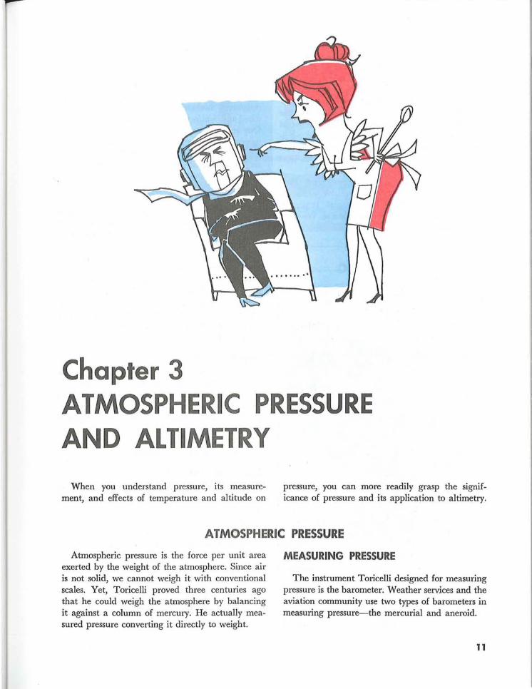
In chapter 1, we learned that temperature nor­mally decreases with increasing altitude throughout the troposphere. This decrease of temperature with altitude is defined as lapse rate. The average de­crease of temperature-average lapse rate-in the troposphere is 2° C per 1,000 feet. But since this is an average, the exact value seldom exists. In fact, temperature sometimes increases with height through a layer. An increase in temperature with altitude is defined as an inv,ersion, i.e., lapse rate is inverted.

An inversion often develops near the ground on clear, cool nights when wind is light. The ground radiates and cools much faster than the overlying air. Air in contact with the ground becomes cold while the temperature a few hundred feet above changes very little. Thus, temperature increases

FIGURE 6. Temperature differences create air movement and, at times, cloudiness.

9

with height. Inversions may also occur at any alti­tude when conditions are favorable . For example, a current of warm air aloft overrunning cold air

near the surface produces an inversion aloft. Figure 7 diagrams temperature inversions both surface and aloft. Inversions are common in the stratosphere.

UP

INVERSION

ALOFT ----

FIGURE 7. Inverted lapse rates or "inversions." A lapse rate is a decrease of temperature with height. An inversion is an increase of temperature with height, i.e., the lapse rate is inverted. Shown here are a surface inversion and an inversion aloft.

IN CLOSING

Temperature affects aircraft performance and is critical to some operations. Following are some op­erational pointers to remember, and most of them are developed in later chapters:

10

1. The aircraft thermometer is subject to in­accuracies no matter how good the instru­ment and its installation. Position of the aircraft relative to the sun can cause errors due to radiation, particularly on a parked aircraft. At high speeds, aerodynamical ef­fects and friction are basically the causes of inaccuracies.

2. High temperature reduces air density and reduces aircraft performance (chapter 3).

3. Diurnal and topographical temperature variations create local winds (chapter 4).

4. Diurnal cooling is conducive to fog (chap­ter 5).

5. Lapse rate contributes to stability (chapter 6) , cloud formation (chapter 7), turbulence (chapter 9), and thunderstorms (chapter 11) .

6. An inversion aloft permits warm rain to fall through cold air below. Temperature in the cold air can be critical to icing (chapter 10) .

7. A ground based inversion favors poor visi­bility by trapping fog, smoke, and other restrictions into low levels of the atmo­sphere ( chapter 12).

Chapter 3 ATMOSPHERIC PRESSURE AND ALTIMETRY

When you understand pressure, its measure­ment, and effects of temperature and altitude on

pressure, you can more readily grasp the signif­icance of pressure and its application to altimetry.

ATMOSPHERIC PRESSURE

Atmospheric pressure is the force per unit area exerted by the weight of the atmosphere. Since air is not solid, we cannot weigh it with conventional scales. Yet, Toricelli proved three centuries ago that he could weigh the atmosphere by balancing it against a column of mercury. He actually mea­sured pressure converting it directly to weight.

MEASURING PRESSURE

The instrument Toricelli designed for measuring pressure is the barometer. Weather services and the aviation community use two types of barometers in measuring pressure-the mercurial and aneroid.

11

The Mercurial Barometer

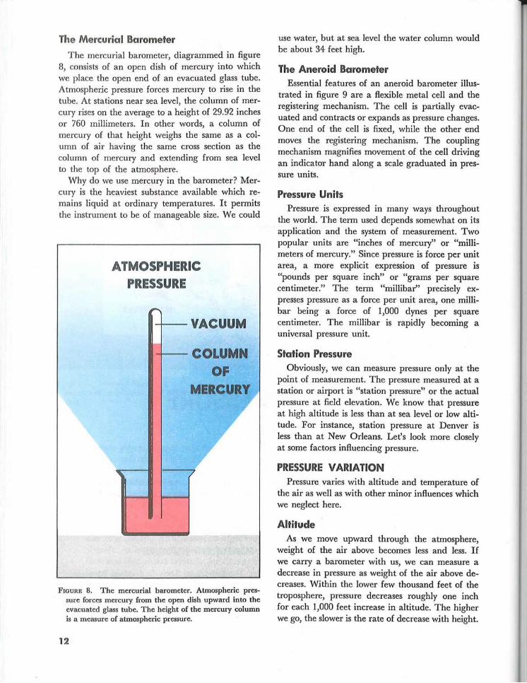
The mercurial barometer, diagrammed in figure 8, consists of an open dish of mercury into which we place the open end of an evacuated glass tube. Atmospheric pressure forces mercury to rise in the tube. At stations near sea level, the column of mer­cury rises on the average to a height of 29.92 inches or 760 millimeters. In other words, a column of mercury of that height weighs the same as a col­umn of air having the same cross section as the column of mercury and extending from sea level to the top of the atmosphere.

Why do we use mercury in the barometer? Mer­cury is the heaviest substance available which re­mains liquid at ordinary temperatures. It permits the instrument to be of manageable size. We could

ATMOSPHERIC PRESSURE

-+--- VACUUM

COLUMN OF

FIGURE 8. The mercurial barometer. Atmospheric pres­sure forces mercury from the open dish upward into the evacuated glass tube. The height of the mercury column is a measure of atmospheric pressure.

12

use water, but at sea level the water column would be about 34 feet high.

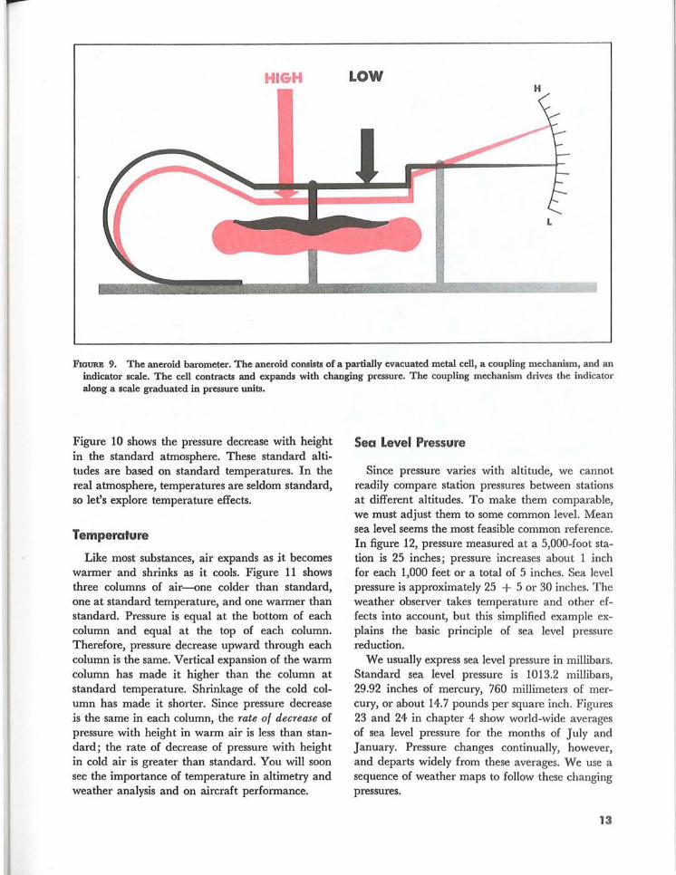
The Aneroid Barometer Essential features of an aneroid barometer illus­

trated in figure 9 are a flexible metal cell and the registering mechanism. The cell is partially evac­uated and contracts or expands as pressure changes. One end of the cell is fixed, while the other end moves the registering mechanism. The coupling mechanism magnifies movement of the cell driving an indicator hand along a scale graduated in pres­sure units.

Pressure Units Pressure is expressed in many ways throughout

the world. The term used depends somewhat on its application and the system of measurement. Two popular units are "inches of mercury" or "milli­meters of mercury." Since pressure is force per unit area, a more explicit expression of pressure is "pounds per square inch" or "grams per square centimeter." The term "millibar" precisely ex­presses pressure as a force per unit area, one milli­bar being a force of 1,000 dynes per square centimeter. The millibar is rapidly becoming a universal pressure unit.

Station Pressure Obviously, we can measure pressure only at the

point of measurement. The pressure measured at a station or airport is "station pressure" or the actual pressure at field elevation. We know that pressure at high altitude is less than at sea level or low alti­tude. For instance, station pressure at Denver is less than at New Orleans. Let's look more closely at some factors influencing pressure.

PRESSURE VARIATION Pressure varies with altitude and temperature of

the air as well as with other minor influences which we neglect here.

Altitude

As we move upward through the atmosphere, weight of the air above becomes less and less. If we carry a barometer with us, we can measure a decrease in pressure as weight of the air above de­creases. Within the lower few thousand feet of the troposphere, pressure decreases roughly one inch for each 1,000 feet increase in altitude. The higher we go, the slower is the rate of decrease with height.

HIGH LOW H

L

FIGURE 9. The aneroid barometer. The aneroid consists of a partially evacuated metal cell, a coupling mechanism, and an indicator scale. The cell contracts and expands with changing pressure. The coupling mechanism drives the indicator along a scale graduated in pressure units.

Figure 10 shows the pressure decrease with height in the standard atmosphere. These standard alti­tudes are based on standard temperatures. In the real atmosphere, temperatures are seldom standard, so let's explore temperature effects.

Temperature

Like most substances, air expands as it becomes warmer and shrinks as it cools. Figure 11 shows three columns of air---one colder than standard, one at standard temperature, and one warmer than standard. Pressure is equal at the bottom of each column and equal at the top of each column. Therefore, pressure decrease upward through each column is the same. Vertical expansion of the warm column has made it higher than the column at standard temperature. Shrinkage of the cold col­umn has made it shorter. Since pressure decrease is the same in each column, the rate of decrease of pressure with height in warm air is less than stan­dard; the rate of decrease of pressure with height in cold air is greater than standard. You will soon see the importance of temperature in altimetry and weather analysis and on aircraft performance.

Sea Level Pressure

Since pressure varies with altitude, we cannot readily compare station pressures between stations at different altitudes. To make them comparable, we must adjust them to some common level. Mean sea level seems the most feasible common reference. In figure 12, pressure measured at a 5,000-foot sta­tion is 25 inches; pressure increases about 1 inch for each 1,000 feet or a total of 5 inches. Sea level pressure is approximately 25 + 5 or 30 inches. The weather observer takes temperature and other ef­fects into account, but this simplified example ex­plains the basic principle of sea level pressure reduction.

We usually express sea level pressure in millibars. Standard sea level pressure is 1013.2 millibars, 29.92 inches of mercury, 760 millimeters of mer­cury, or about 14.7 pounds per square inch. Figures 23 and 24 in chapter 4 show world-wide averages of sea level pressure for the months of July and January. Pressure changes continually, however, and departs widely from these averages. We use a sequence of weather maps to follow these changing pressures.

13

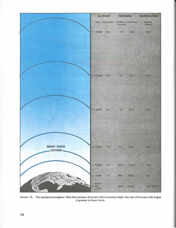
FIGURE 10. The standard atmosphere. Note how pressure decreases with increasing height; the rate of decrease with height is greatest in lower levels.

14

WARM STANDARD

COLD

FIGURE 11. Three columns of air showing how decrease of pressure with height varies with temperature. Left column is colder than average and right column, warmer than average. Pressure is equal at the bottom of each column and equal at the top of each column. Pressure decreases most rapidly with height in the cold air and least rapidly in the warm air.

Pressure Analyses

We plot sea level pressures on a map and draw lines connecting points of equal pressure. These lines of equal pressure are isobars. Hence, the sur­face map is an isobaric analysis showing identifi-

A Pressure

at 5000' of '25 INCHES

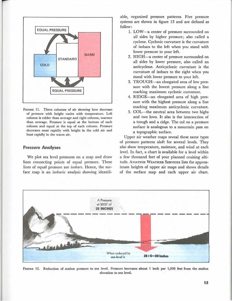
able, organized pressure patterns. Five pressure systems are shown in figure 13 and are defined as follow:

1. LOW-a center of pressure surrounded on all sides by higher pressure; also called a cyclone. Cyclonic curvature is the curvature of isobars to the left when you stand with lower pressure to your left.

2. HIGH-a center of pressure surrounded on all sides by lower pressure, also called an anticyclone. Anticyclonic curvature is the curvature of isobars to the right when you stand with lower pressure to your left.

3. TROUGH-an elongated area of low pres­sure with the lowest pressure along a line marking maximum cyclonic curvature.

4. RIDGE-an elongated area of high pres­sure with the highest pressure along a line marking maximum anticyclonic curvature.

5. COL-the neutral area between two highs and two lows. It also is the intersection of a trough and a ridge. The colon a pressure surface is analogous to a mountain pass on a topographic surface.

Upper air weather maps reveal these same types of pressure patterns aloft for several levels. They also show temperature, moisture, and wind at each level. In fact, a chart is available for a level within a few thousand feet of your planned cruising alti­tude. AVIATION WEATHER SERVICES lists the approx­imate heights of upper air maps and shows details of the surface map and each upper air chart.

-----------0::..::=_---------

When reduced to sea-level is 25+5=30 Inches

FIGURE 12. Reduction of .station pressure to sea level. Pressure increases about 1 inch per 1,000 feet from the station elevation to sea level.

15

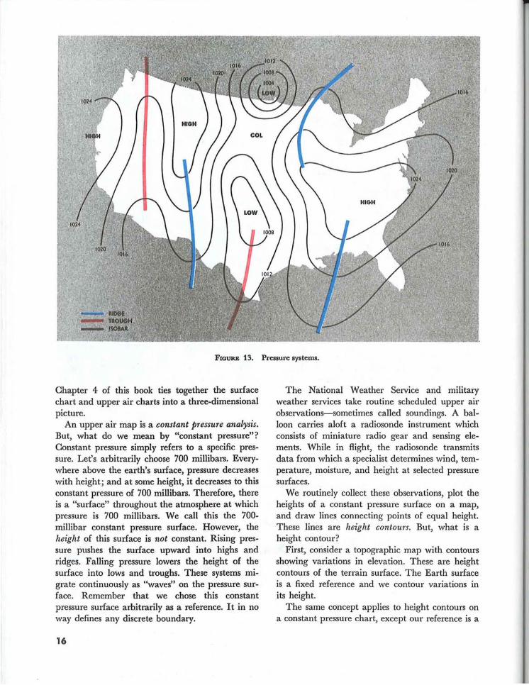
FIGURE 13. Pressure systems.

Chapter 4 of this book ties together the surface chart and upper air charts into a three-dimensional picture.

An upper air map is a constant pressure analysis. But, what do we mean by "constant pressure"? Constant pressure simply refers to a specific pres­sure. Let's arbitrarily choose 700 m.illibars. Every­where above the earth's surface, pressure decreases with height; and at some height, it decreases to this constant pressure of 700 millibars. Therefore, there is a "surface" throughout the atmosphere at which pressure is 700 millibars. We call this the 700-m.illibar constant pressure surface. However, the height of this surface is not constant. Rising pres­sure pushes the surface upward into highs and ridges. Falling pressure lowers the height of the surface into lows and troughs. These systems mi­grate continuously as "waves" on the pressure sur­face. Remember that we chose this constant pressure surface arbitrarily as a reference. It in no way defines any discrete boundary.

16

The National Weather Service and military weather services take routine scheduled upper air observations-sometimes called soundings. A bal­loon carries aloft a radiosonde instrument wh.ich consists of miniature radio gear and sensing ele­ments. While in flight, the radiosonde transmits data from which a specialist determines wind, tem­perature, moisture, and height at selected pressure surfaces.

We routinely collect these observations, plot the heights of a constant pressure surface on a map, and draw lines connecting points of equal height. These lines are height contours. But, what is a height contour?

First, consider a topographic map with contours showing variations in elevation. These are height contours of the terrain surface. The Earth surface is a fixed reference and we contour variations in its height.

The same concept applies to height contours on a constant pressure chart, except our reference is a

constant pressure surface. We simply contour the heights of the pressure surface. For example, a 700-millibar constant pressure analysis is a contour map of the heights of the 700-millibar pressure sur­face. While the contour map is based on variations in height, these variations are small when com­pared to flight levels, and for all practical pur­poses, you may regard the 700-millibar chart as a weather map at approximately 10,000 feet or 3,048 meters.

A contour analysis shows highs, ridges, lows, and troughs aloft just as the isobaric analysis shows such systems at the surface. What we say concerning

pressure patterns and systems applies equally to an isobaric or a contour analysis.

Low pressure systems quite often are regions of poor flying weather, and high pressure areas pre­dominantly are regions of favorable flying weather. A word of caution, however-use care in applying the low pressure-bad weather, high pressure-good weather rule of thumb; it all too frequently fails. When planning a flight, gather all information pos­sible on expected weather. Pressure patterns also bear a direct relationship to wind which is the sub­ject of the next chapter. But first, let's look at pres­sure and altimeters.

ALTIMETRY

The altimeter is essentially an aneroid barometer. The difference is the scale. The altimeter is grad­uated to read increments of height rather than units of pressure. The standard for graduating the altimeter is the standard atmosphere.

ALTITUDE Altitude seems like a simple term; it means

height. But in aviation, it can have many meanings.

True Altitude Since existing conditions in a real atmosphere

are seldom standard, altitude indications on the altimeter are seldom actual or true altitudes. True altitude is the actual or exact altitude above mean sea level. If your altimeter does not indicate true altitude, what does it indicate?

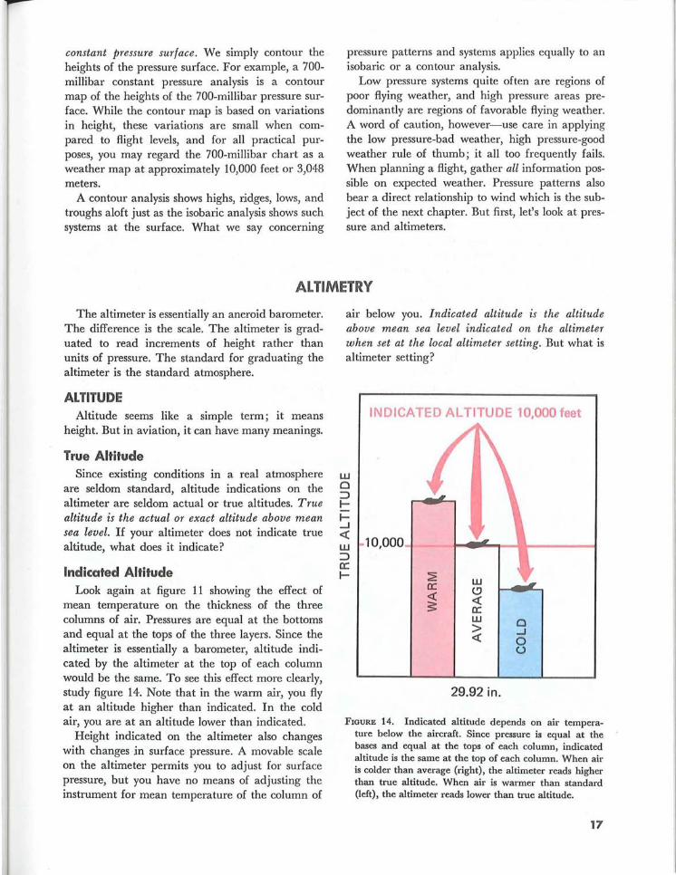
Indicated Altitude Look again at figure 11 showing the effect of

mean temperature on the thickness of the three columns of air. Pressures are equal at the bottoms and equal at the tops of the three layers. Since the altimeter is essentially a barometer, altitude indi­cated by the altimeter at the top of each column would be the same. To see this effect more clearly, study figure 14. Note that in the warm air, you fly at an altitude higher than indicated. In the cold air, you are at an altitude lower than indicated.

Height indicated on the altimeter also changes with changes in surface pressure. A movable scale on the altimeter permits you to adjust for surface pressure, but you have no means of adjusting the instrument for mean temperature of the column of

air below you. Indicated altitude is the altitude above mean sea level indicated on the altimeter when set at the local altimeter setting. But what is altimeter setting?

w o :::::> l-I­~

« w :::::> a:: I-

INDICATED ALTITUDE 10,000 feet

10,000

LU (!)

« a: LU > «

29.92 in.

o ~

o u

FIGURE 14. Indicated altitude depends on air tempera­ture below the aircraft. Since pressure is equal at the bases and equal at the tops of each column, indicated altitude is the same at the top of each column. When air is colder than average (right), the altimeter reads higher than true altitude. When air is warmer than standard (left), the altimeter reads lower than true altitude.

17

r

Altimeter Setting

Since the altitude scale is adjustable, you can set the altimeter to read true altitude at some specified height. Takeoff and landing are the most critical phases of flight; therefore, airport elevation is the most desirable altitude for a true reading of the altimeter. Altimeter setting is the value to which the scale of the pressure altimeter is set so the al­timeter indicates true altitude at field elevation.

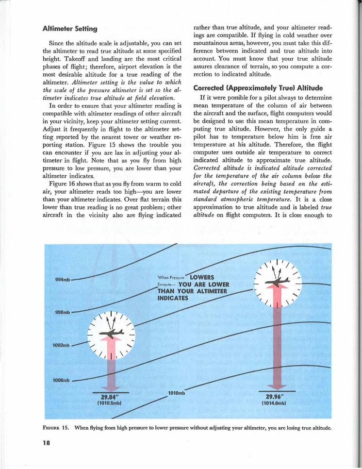
In order to ensure that your altimeter reading is compatible with altimeter readings of other aircraft in your vidnity, keep your altimeter setting current. Adjust it frequently in flight to the altimeter set­ting reported by the nearest tower or weather re­porting station. Figure 15 shows the trouble you can encounter if you are lax in adjusting your al­timeter in flight. Note that as you fly from high pressure to low pressure, you are lower than your altimeter indicates.

Figure 16 shows that as you fly from warm to cold air, your altimeter reads too high-you are lower than your altimeter indicates. Over flat terrain this lower than true reading is no great problem; other aircraft in the vicinity also are flying indicated

rather than true altitude, and your altimeter read­ings are compatible. If flying in cold weather over mountainous areas, however, you must take this dif­ference between indicated and true altitude into account. You must know that your true altitude assures clearance of terrain, so you compute a cor­rection to indicated altitude.

Corrected (Approximately True) Altitude If it were possible for a pilot always to determine

mean temperature of the column of air between the aircraft and the surface, flight computers would be designed to use this mean temperature in com­puting true altitude. However, the only guide a pilot has to temperature below him is free air temperature at his altitude. Therefore, the flight computer uses outside air temperature to correct indicated altitude to approximate true altitude. Corrected altitude is indicated altitude corrected for the temperature of the air column below the aircraft, the correction being based on the esti­mated departure of the existing temperature from standard atmospheric temperature. It is a close approximation to true altitude and is labeled true altitude on flight computers. It is close enough to

'94mb~>"'. LOWERS

998mb

1006mb

Enroute- YOU ARE LOWER THAN YOUR ALTIMETER INDICATES

29.85~~) ~ 1010mb

(1010./

" / \ ' I 1\

29.96" (1014.6mb)

FIGURE 15. When flying from high pressure to lower pressure without adjusting your altimeter, you are losing true altitude.

18

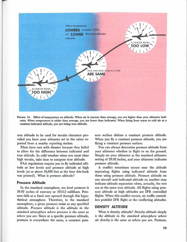
When temperoture

LOWERS enroufe;=Y.OU

\ I I , \ \0 / / " I /' are LOWER thon yOQ,l" lIlt Jrn:rs:ter ~ 7 ~ I 2 ... < ___ _

indicates

ALTIMETER READS -

/'TOO LOW' / ,

I I I \ \

TRUE AND INDICATED ALTITUDE

ARE SAME I \ \ "

FIGURE t 6. Effect of temperature on altitude. When air is warmer than average, you are higher than your altimeter indi­cates. When temperature is colder than average, you are lower than indicated. When flying from warm to cold air at a constant indicated altitude, you are losing true altitude.

true altitude to be used for terrain clearance pro­vided you have your altimeter set to the value re­ported from a nearby reporting station.

Pilots have met with disaster because they failed to allow for the difference between indicated and true altitude. In cold weather when you must clear high terrain, take time to compute true altitude.

FAA regulations require you to fly indicated alti­tude at low levels and pressure altitude at high levels (at or above 18,000 feet at the time this book was printed). What is pressure altitude?

Pressure Altitude In the standard atmosphere, sea level pressure is

29.92 inches of mercury or 1013.2 millibars. Pres­sure falls at a fixed rate upward through this hypo­thetical atmosphere. Therefore, in the standard atmosphere, a given pressure exists at any specified altitude. Pressure altitude is the altitude in the standard atmosphere where pressure is the same as where you are. Since at a specific pressure altitude, pressure is everywhere the same, a constant pres-

sure surface defines a constant pressure altitude. When you fly a constant pressure altitude, you are flying a constant pressure surface.

You can always determine pressure altitude from your altimeter whether in flight or on the ground. Simply set your altimeter at the standard altimeter setting of 29.92 inches, and your altimeter indicates pressure altitude.

A conflict sometimes occurs near the altitude separating flights using indicated altitude from those using pressure altitude. Pressure altitude on one aircraft and indicated altitude on another may indicate altitude separation when, actually, the two are at the same true altitude. All flights using pres­sure altitude at high altitudes are IFR controlled flights. When this conflict occurs, air traffic control­lers prohibit IFR flight at the conflicting altitudes.

DENSITY ALTITUDE What is density altitude? Density altitude simply

is the altitude in the standard atmosphere where air density is the same as where you are. Pressure,

19

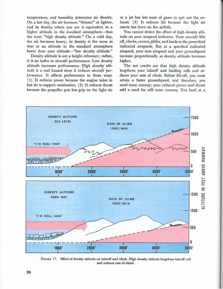
temperature, and humidity determine air density. On a hot day, the air becomes "thinner" or lighter, and its density where you are is equivalent to a higher altitude in the standard atmosphere-thus the term "high density altitude." On a cold day, the air becomes heavy; its density is the same as that at an altitude in the standard atmosphere lower than your altitude-"low density altitude."

Density altitude is not a height reference; rather, it is an index to aircraft performance. Low density altitude increases performance. High density alti­tude is a real hazard since it reduces aircraft per­formance. It affects performance in three ways. (1) It reduces power because the engine takes in less air to support combustion. (2) It reduces thrust because the propeller gets less grip on the light air

DENSITY ALTITUDE

SEA LEVEL

or a jet has less mass of gases to spit out the ex­haust. (3) It reduces lift because the light air exerts less force on the airfoils.

You cannot detect the effect of high density alti­tude on your airspeed indicator. Your aircraft lifts off, climbs, cruises, glides, and lands at the prescribed indicated airspeeds. But at a specified indicated airspeed, your true airspeed and your groundspeed increase proportionally as density altitude becomes higher.

The net results are that high density altitude lengthens your takeoff and landing rolls and re­duces your rate of climb. Before lift-off, you must attain a faster groundspeed, and therefore, you need more runway; your reduced power and thrust add a need for still more runway. You land at a

1500 RATE OF CLIMB

1300' / MIN ..".. -- 1000 / --

T / 0 ROLL 1300'

- 500

... _ ... -2000' 3000' 4000'

DENSITY ALTITUDE 1500 5000 FEET

RA TE OF CLI MB

1000' /MI N

1000 T/O ROLL 1800'

500 ------------------r--- --- 0

20

1000' 2000' 3000' 4000' 5000'

FIGURE 17. Effect of density altitude on takeoff and climb. High density altitude lengthens takeoff roll and reduces rate of climb.

>-cc ~ Z :::l a::: ..... > Q QO < ~ ..... ..... ...... Z

..... c ::I ~

~ -J cc

faster groundspeed and, therefore, need more room to stop. At a prescribed indicated airspeed, you are flying at a faster true airspeed, and therefore, you cover more distance in a given time which means climbing at a more shallow angle. Add to this the problems of reduced power and rate of climb, and you are in double jeopardy in your climb. Figure 17 shows the effect of density altitude on takeoff distance and rate of climb.

High density altitude also can be a problem at cruising altitudes. When air is abnormally warm, the high density altitude lowers your service ceiling. For example, if temperature at 10,000 feet pres­sure altitude is 20° C, density altitude is 12,700

feet. (Check this on your flight computer.) Your aircraft will perform as though it were at 12,700 indicated with a normal temperature of _8° C.

To compute density altitude, set your altimeter at 29.92 inches or 1013.2 millibars and read pres­sure altitude from your altimeter. Read outside air temperature and then use your flight computer to get density altitude. On an airport served by a weather observing station, you usually can get den­sity altitude for the airport from the observer. Sec­tion 16 of AVIATION WEATHER SERVICES has a graph for computing density altitude if you have no flight computer handy.

IN CLOSING

Pressure patterns can be a clue to weather causes and movement of weather systems, but they give only a part of the total weather picture. Pressure decreases with increasing altitude. The altimeter is an aneroid barometer graduated in increments of altitude in the standard atmosphere instead of units of pressure. Temperature greatly affects the rate of pressure decrease with height; therefore, it influ­ences altimeter readings. Temperature also deter­mines the density of air at a given pressure (density altitude). Density altitude is an index to aircraft performance. Always be alert for departures of pressure and temperature from normals and com­pensate for these abnormalities.

Following are a few operational reminders: 1. Beware of the low pressure-bad weather,

high pressure-good weather rule of thumb. It frequently fails. Always get the complete weather picture.

2. When flying from high pressure to low pres­sure at constant indicated altitude and with­out adjusting the altimeter, you are losing true altitude.

3. When temperature is colder than standard, you are at an altitude lower than your al­timeter indicates. When temperature is warmer than standard, you are higher than your altimeter indicates.

4. When flying cross country, keep your altim­eter setting current. This procedure assures more positive altitude separation from other aircraft.

5. When flying over high terrain in cold weather, compute your true altitude to en­sure terrain clearance.

6. When your aircraft is heavily loaded, the temperature is abnormally warm, and/or the pressure is abnormally low, compute density altitude. Then check your aircraft manual to ensure that you can become air­borne from the available runway. Check further to determine that your rate of climb permits clearance of obstacles beyond the end of the runway. This procedure is ad­visable for any airport regardless of altitude.

7. When planning takeoff or landing at a high altitude airport regardless of load, determine density altitude. The procedure is especially critical when temperature is abnormally warm or pressure abnormally low. Make certain you have sufficient run­way for takeoff or landing roll. Make sure you can clear obstacles beyond the end of the runway after takeoff or in event of a go-around.

8. Sometimes the altimeter setting is taken from an instrument of questionable reli­ability. However, if the instrument can cause an error in altitude reading of more than 20 feet, it is removed from service. When altimeter setting is estimated, be pre­pared for a possible 10- to 20-foot differ­ence between field elevation and your al­timeter reading at touchdown.

21