Appendix: Supplementary Material
A Mathematical Proofs
A.1 Preliminaries
We shall use the notations Re(z) and Im(z) for the real and imaginary parts of a complex
number z, so that
∀z ∈ C z = Re(z) + i · Im(z) .
For any increasing function G on the real line, sG denotes the Stieltjes transform of G:
∀z ∈ C+ sG(z) ..=
!1
λ− zdG(λ) .
The Stieltjes transform admits a well-known inversion formula:
G(b)−G(a) = limη→0+
1
π
! b
aIm"sG(ξ + iη)
#dξ , (A.1)
as long as G is continuous at both a and b. Bai and Silverstein (2010, p.112) give the following
version for the equation that relates F to H and c. The quantity s =.. sF (z) is the unique
solution in the set $s ∈ C : −
1− c
z+ cs ∈ C
+
%(A.2)
to the equation
∀z ∈ C+ s =
!1
τ"1− c− c z s
#− z
dH(τ) . (A.3)
Although the Stieltjes transform of F , sF , is a function whose domain is the upper half of the
complex plane, it admits an extension to the real line ∀x ∈ R \ {0} sF (x) ..= limz∈C+→x sF (z)
which is continuous over x ∈ R− {0}. When c < 1, sF (0) also exists and F has a continuous
derivative F ′ = π−1Im [sF ] on all of R with F ′ ≡ 0 on (−∞, 0]. (One should remember that,
although the argument of sF is real-valued now, the output of the function is still a complex
number.)
Recall that the limiting e.d.f. of the eigenvalues of n−1Y ′nYn = n−1Σ1/2
n X ′nXnΣ
1/2n was
defined as F . In addition, define the limiting e.d.f. of the eigenvalues of n−1YnY ′n =
n−1XnΣnX ′n as F ; note that the eigenvalues of n−1Y ′
nYn and n−1YnY ′n only differ by |n − p|
zero eigenvalues. It then holds:
∀x ∈ R F (x) = (1− c) [0,∞)(x) + c F (x) (A.4)
∀x ∈ R F (x) =c− 1
c [0,∞)(x) +1
cF (x) (A.5)
∀z ∈ C+ sF (z) =
c− 1
z+ c sF (z) (A.6)
∀z ∈ C+ sF (z) =
1− c
c z+
1
csF (z) . (A.7)
1
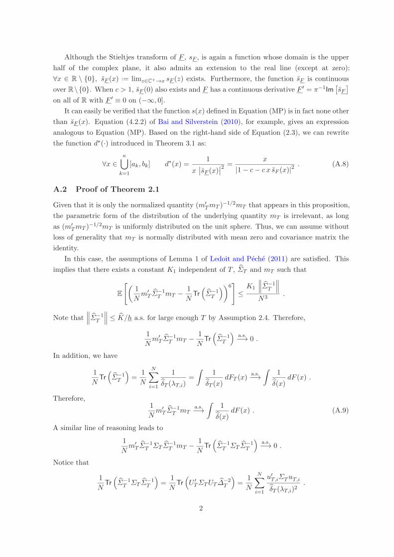
Although the Stieltjes transform of F , sF , is again a function whose domain is the upper
half of the complex plane, it also admits an extension to the real line (except at zero):
∀x ∈ R \ {0}, sF (x) ..= limz∈C+→x sF (z) exists. Furthermore, the function sF is continuous
over R\{0}. When c > 1, sF (0) also exists and F has a continuous derivative F ′ = π−1Im"sF#
on all of R with F ′ ≡ 0 on (−∞, 0].
It can easily be verified that the function s(x) defined in Equation (MP) is in fact none other
than sF (x). Equation (4.2.2) of Bai and Silverstein (2010), for example, gives an expression
analogous to Equation (MP). Based on the right-hand side of Equation (2.3), we can rewrite
the function d∗(·) introduced in Theorem 3.1 as:
∀x ∈κ&
k=1
[ak, bk] d∗(x) =1
x''sF (x)
''2=
x
|1− c− c x sF (x)|2 . (A.8)
A.2 Proof of Theorem 2.1
Given that it is only the normalized quantity (m′
TmT )−1/2mT that appears in this proposition,
the parametric form of the distribution of the underlying quantity mT is irrelevant, as long
as (m′
TmT )−1/2mT is uniformly distributed on the unit sphere. Thus, we can assume without
loss of generality that mT is normally distributed with mean zero and covariance matrix the
identity.
In this case, the assumptions of Lemma 1 of Ledoit and Peche (2011) are satisfied. This
implies that there exists a constant K1 independent of T , (ΣT and mT such that
E
)*1
Nm′
T(Σ−1T mT −
1
NTr+(Σ−1T
,-6.
≤K1
/// (Σ−1T
///
N3.
Note that/// (Σ−1
T
/// ≤ (K/h a.s. for large enough T by Assumption 2.4. Therefore,
1
Nm′
T(Σ−1T mT −
1
NTr+(Σ−1T
,a.s.−→ 0 .
In addition, we have
1
NTr+(Σ−1T
,=
1
N
N0
i=1
1(δT (λT,i)
=
!1
(δT (x)dFT (x)
a.s.−→
!1(δ(x)
dF (x) .
Therefore,1
Nm′
T(Σ−1T mT
a.s.−→
!1(δ(x)
dF (x) . (A.9)
A similar line of reasoning leads to
1
Nm′
T(Σ−1T ΣT
(Σ−1T mT −
1
NTr+(Σ−1T ΣT
(Σ−1T
,a.s.−→ 0 .
Notice that
1
NTr+(Σ−1T ΣT
(Σ−1T
,=
1
NTr+U ′
TΣTUT(∆−2T
,=
1
N
N0
i=1
u′T,iΣTuT,i(δT (λT,i)2
.
2
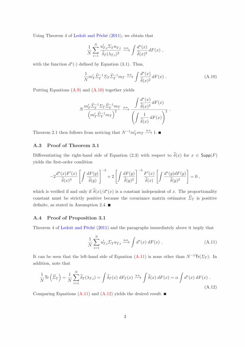
Using Theorem 4 of Ledoit and Peche (2011), we obtain that
1
N
N0
i=1
u′T,iΣTuT,i(δT (λT,i)2
a.s.−→
!d∗(x)(δ(x)2
dF (x) ,
with the function d∗(·) defined by Equation (3.1). Thus,
1
Nm′
T(Σ−1T ΣT
(Σ−1T mT
a.s.−→
!d∗(x)(δ(x)2
dF (x) . (A.10)
Putting Equations (A.9) and (A.10) together yields
Nm′
T(Σ−1T ΣT
(Σ−1T mT
+m′
T(Σ−1T mT
,2a.s.−→
!d∗(x)(δ(x)2
dF (x)
1!1(δ(x)
dF (x)
22 .
Theorem 2.1 then follows from noticing that N−1m′
TmTa.s.−→ 1.
A.3 Proof of Theorem 3.1
Differentiating the right-hand side of Equation (2.3) with respect to (δ(x) for x ∈ Supp(F )
yields the first-order condition
−2d∗(x)F ′(x)(δ(x)3
)!dF (y)(δ(y)
.−2
+ 2
)!dF (y)(δ(y)2
.−3F ′(x)(δ(x)
)!d∗(y)dF (y)(δ(y)2
.
= 0 ,
which is verified if and only if (δ(x)/d∗(x) is a constant independent of x. The proportionality
constant must be strictly positive because the covariance matrix estimator (ΣT is positive
definite, as stated in Assumption 2.4.
A.4 Proof of Proposition 3.1
Theorem 4 of Ledoit and Peche (2011) and the paragraphs immediately above it imply that
1
N
N0
i=1
u′T,iΣTuT,ia.s.−→
!d∗(x) dF (x) . (A.11)
It can be seen that the left-hand side of Equation (A.11) is none other than N−1Tr(ΣT ). In
addition, note that
1
NTr+(ΣT
,=
1
N
N0
i=1
(δT (λT,i) =
!(δT (x) dFT (x)
a.s.−→
!(δ(x) dF (x) = α
!d∗(x) dF (x) .
(A.12)
Comparing Equations (A.11) and (A.12) yields the desired result.
3
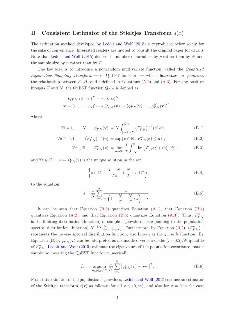
B Consistent Estimator of the Stieltjes Transform s(x)
The estimation method developed by Ledoit and Wolf (2015) is reproduced below solely for
the sake of convenience. Interested readers are invited to consult the original paper for details.
Note that Ledoit and Wolf (2015) denote the number of variables by p rather than by N and
the sample size by n rather than by T .
The key idea is to introduce a nonrandom multivariate function, called the Quantized
Eigenvalues Sampling Transform — or QuEST for short — which discretizes, or quantizes,
the relationship between F , H, and c defined in Equations (A.2) and (A.3). For any positive
integers T and N , the QuEST function QT,N is defined as
QT,N : [0,∞)N −→ [0,∞)N
v ..= (v1, . . . , vN )′ (−→ QT,N (v) ..=3q1T,N (v), . . . , qNT,N (v)
4′,
where
∀i = 1, . . . , N qiT,N (v) ..= N
! i/N
(i−1)/N
3FvT,N
4−1(u) du , (B.1)
∀u ∈ [0, 1]3FvT,N
4−1(u) ..= sup{x ∈ R : Fv
T,N (x) ≤ u} , (B.2)
∀x ∈ R FvT,N (x) ..= lim
η→0+
1
π
! x
−∞
Im"svT,N (ξ + iη)
#dξ , (B.3)
and ∀z ∈ C+ s ..= svT,N (z) is the unique solution in the set
$s ∈ C : −
T −N
Tz+
N
Ts ∈ C
+
%(B.4)
to the equation
s =1
N
N0
i=1
1
vi
*1−
N
T−
N
Tz s
-− z
. (B.5)
It can be seen that Equation (B.3) quantizes Equation (A.1), that Equation (B.4)
quantizes Equation (A.2), and that Equation (B.5) quantizes Equation (A.3). Thus, FvT,N
is the limiting distribution (function) of sample eigenvalues corresponding to the population
spectral distribution (function) N−15Ni=1 [vi,∞). Furthermore, by Equation (B.2),
3FvT,N
4−1
represents the inverse spectral distribution function, also known as the quantile function. By
Equation (B.1), qiT,N (v) can be interpreted as a smoothed version of the (i− 0.5)/N quantile
of FvT,N . Ledoit and Wolf (2015) estimate the eigenvalues of the population covariance matrix
simply by inverting the QuEST function numerically:
(τT ..= argminv∈(0,∞)N
1
N
N0
i=1
"qiT,N (v)− λT,i
#2. (B.6)
From this estimator of the population eigenvalues, Ledoit and Wolf (2015) deduce an estimator
of the Stieltjes transform s(x) as follows: for all x ∈ (0,∞), and also for x = 0 in the case
4
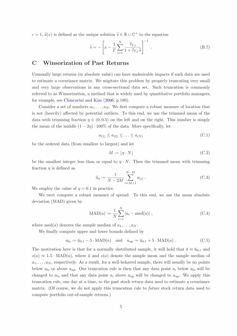
c > 1, (s(x) is defined as the unique solution (s ∈ R ∪ C+ to the equation
(s = −
)
x−1
T
N0
i=1
(τT,i1 + (τT,i (s
.−1
. (B.7)
C Winsorization of Past Returns
Unusually large returns (in absolute value) can have undesirable impacts if such data are used
to estimate a covariance matrix. We migitate this problem by properly truncating very small
and very large observations in any cross-sectional data set. Such truncation is commonly
referred to as Winsorization, a method that is widely used by quantitative portfolio managers;
for example, see Chincarini and Kim (2006, p.180).
Consider a set of numbers a1, . . . , aN . We first compute a robust measure of location that
is not (heavily) affected by potential outliers. To this end, we use the trimmed mean of the
data with trimming fraction η ∈ (0, 0.5) on the left and on the right. This number is simply
the mean of the middle (1− 2η) · 100% of the data. More specifically, let
a(1) ≤ a(2) ≤ . . . ≤ a(N) (C.1)
be the ordered data (from smallest to largest) and let
M ..= ⌊η ·N⌋ (C.2)
be the smallest integer less than or equal to η · N . Then the trimmed mean with trimming
fraction η is defined as
aη ..=1
N − 2M
N−M0
i=M+1
a(i) . (C.3)
We employ the value of η = 0.1 in practice.
We next compute a robust measure of spread. To this end, we use the mean absolute
deviation (MAD) given by
MAD(a) ..=1
N
N0
i=1
|ai −med(a)| , (C.4)
where med(a) denotes the sample median of a1, . . . , aN .
We finally compute upper and lower bounds defined by
alo ..= a0.1 − 5 ·MAD(a) and aup ..= a0.1 + 5 ·MAD(a) . (C.5)
The motivation here is that for a normally distributed sample, it will hold that a ≈ a0.1 and
s(a) ≈ 1.5 · MAD(a), where a and s(a) denote the sample mean and the sample median of
a1, . . . , aN , respectively. As a result, for a well-behaved sample, there will usually be no points
below alo or above aup. Our truncation rule is then that any data point ai below alo will be
changed to alo and that any data point ai above aup will be changed to aup. We apply this
truncation rule, one day at a time, to the past stock return data used to estimate a covariance
matrix. (Of course, we do not apply this truncation rule to future stock return data used to
compute portfolio out-of-sample returns.)
5
D Markowitz Portfolio with Momentum Signal
We now turn attention to a full Markowitz portfolio with a signal, thereby augmenting the
empirical results of Section 4.3 for the global mininum-variance portfolio.
As discussed at the beginning of Section 1, by now a large number of variables have
been documented that can be used to construct a signal in practice. For simplicity and
reproducibility, we use the well-known momentum factor — or simply momentum for short —
of Jegadeesh and Titman (1993). For a given period investment period h and a given stock,
momentum is the geometric average of the previous 12 monthly returns on the stock but
excluding the most recent month. Collecting the individual momentums of all the N stocks
contained in the portfolio universe yields the return predictive signal m.
In the absence of short-sales constraints, the investment problem is formulated as
minw
w′Σw (D.1)
subject to w′m = b and w′1 = 1 , (D.2)
where b is a selected target expected return. The analytical solution of the problem is given in
Sections 3.8 and 3.9 of the textbook by Huang and Litzenberger (1988). The natural strategy
in practice is to replace the unknown Σ by an estimator (Σ, yielding a feasible portfolio
(w ..=Cb−A
BC −A2(Σ−1m+
B −Ab
BC −A2(Σ−11 , (D.3)
where A ..= m′ (Σ−11 , B ..= m′ (Σ−1m , and C ..= 1′ (Σ−11 . (D.4)
The following 12 portfolios are included in the study.
• EW-TQ: The equal-weighted portfolio of the top-quintile stocks according to momen-
tum m. This strategy does not make use of the momentum signal beyond sorting of the
stocks in quintiles.
The value of the target expected return b for portfolios listed below is then given by the
arithmetic average of the momentums of the stocks included in this portfolio (i.e., the
expected return of EW-TQ according to the signal m).
• BSV: The portfolio (D.3)–(D.4) where (Σ is given by the identity matrix of dimension
N ×N . This portfolio corresponds to the proposal of Brandt et al. (2009).
• Sample: The portfolio (D.3)–(D.4) where (Σ is given by the sample covariance matrix;
note that this portfolio is not available when N > T , since the sample covariance matrix
is not invertible in this case.
• KZ: The three-fund portfolio described by Equation (68) of Kan and Zhou (2007); note
that this portfolio is not available when N ≥ T − 4.
This portfolio uses the vector of sample means as signal. For a fair comparison with
other portfolios, we also compute alternative performance measures where the vector of
sample means is replaced by the momentum signal.1
1As the mathematical derivation of the KZ portfolio is based on the vector of sample means as signal, the
modification using the momentum signal is of purely heuristic nature.
6
• TZ: The three-fund portfolio KZ combined with the equal-weighted portfolio as proposed
in Section 2.3 of Tu and Zhou (2011); note that this portfolio is not available when
N ≥ T − 4.
This portfolio uses the vector of sample means as signal. For a fair comparison with
other portfolios, we also compute alternative performance measures where the vector of
sample means is replaced by the momentum signal.2
• Lin: The portfolio (D.3)–(D.4) where (Σ is given by the linear shrinkage estimator of
Ledoit and Wolf (2004).
• NonLin: The portfolio (D.3)–(D.4) where (Σ is given by the estimator (S of Corollary 3.1.
• NL-Inv: The portfolio (D.3)–(D.4) where (Σ−1 is given by the direct nonlinear shrinkage
estimator of Σ−1 based on generic a Frobenius-norm loss. This estimator was first
suggested by Ledoit and Wolf (2012) for the case N < T ; the extension to the case
T ≥ N can be found in Ledoit and Wolf (2018).
• SF: The portfolio (D.3)–(D.4) where (Σ is given by the single-factor covariance matrix(ΣF used in the construction of the single-factor-preconditioned nonlinear shrinkage
estimator (4.1).
• FF: The portfolio (D.3)–(D.4) where (Σ is given by the covariance matrix estimator based
on the (exact) three-factor model of Fama and French (1993).3
• POET: The portfolio (D.3)–(D.4) where (Σ is given by the POET covariance matrix
estimator of Fan et al. (2013). This method uses an approximate factor model where the
factors are taken to be the principal components of the sample covariance matrix and
thresholding is applied to covariance matrix of the principal orthogonal complements.4
• NL-SF The portfolio (D.3)–(D.4) where (Σ is given by the single-factor-preconditioned
nonlinear shrinkage estimator (4.1).
Remark D.1 (KZ and TZ Portfolios). The two portfolios KZ and TZ are not directly
comparable to the other nine portfolios, since they are not fully invested in stocks; instead
they are partly invested in the risk-free rate.
A further issue is that the original proposals for KZ and TZ use the vector of sample
means as the signal unlike the other nine portfolios which use the momentum signal. This
discrepancy might result in an unfair comparison. Therefore, we always present two numbers
for the portfolios KZ and TZ: The first number is based on the vector of sample means as
signal and the second number is based on the momentum signal (i.e., the same signal as used
by the other nine portfolios). Note that there is no theoretical justification for the second set
of numbers and it is purely heuristic approach on our part in the interest of fairness in the
sense of using a shared signal across all portfolios.
2As the mathematical derivation of the TZ portfolio is based on the vector of sample means as signal, the
modification using the momentum signal is purely heuristic.3Data on the three Fama-French factors were downloaded from Ken French’s Data Library.4In particular, we use K = 5 factors, soft thresholding, and the value of C = 1.0 for the thresholding
parameter. Among several specifications we tried, this one appeared to work best on average.
7

Our stance is that in the context of a full Markowitz portfolio, the most important
performance measure is the out-of-sample Sharpe ratio, SR. In the ideal investment problem
(D.1)–(D.2), minimizing the variance (for a fixed target expected return b) is equivalent to
maximizing the Sharpe ratio (for a fixed target expected return b). In practice, because of
estimation error in the signal, the various strategies do not have the same expected return;
thus, focusing on the out-of-sample standard deviation is inappropriate.
We also consider the question whether one portfolio delivers a higher out-of-sample Sharpe
ratio than another portfolio at a level that is statistically significant. Since we consider 12
portfolios, there are 66 pairwise comparisons. To avoid a multiple-testing problem and since
a major goal of this paper is to show that nonlinear shrinkage improves upon linear shrinkage
in portfolio selection, we restrict attention to the single comparison between the two portfolios
Lin and NonLin. For a given scenario, a two-sided p-value for the null hypothesis of equal
Sharpe ratios is obtained by the prewhitened HACPW method described in Ledoit and Wolf
(2008, Section 3.1).5
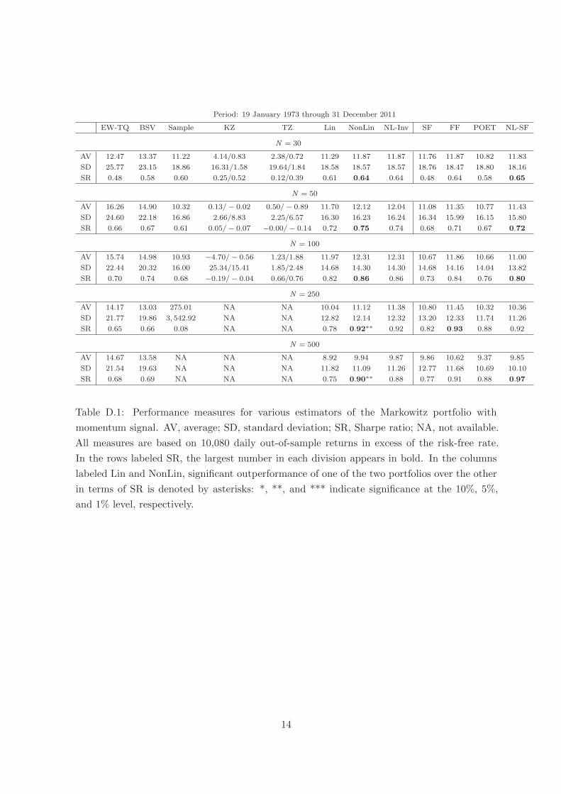
Table D.1 reports the results, which can be summarized as follows.
• We again observe that Sample breaks down for N = 250, when the sample covariance
matrix is close to singular.
• KZ and TZ have the lowest Sharpe ratios throughout and some of the numbers are even
negative.
• The overall order, from worst to best, of the remaining five rotation-equivariant portfolios
is EW-TQ, BSV, Lin, NL-Inv, and NonLin.
• NonLin has the uniformly best performance among the rotation-equivariant portfolios
and the outperformance over Lin is statistically significant at the 0.05 level for N =
250, 500.
• The outperformance is also economically significant for N = 250 and 500, as it is of the
order of a 0.15 increase in the Sharpe ratio. This means the Sharpe ratio goes up by
about one-fifth of its original level, which in the industry would be considered a valuable
improvement.
• Among the four factor-based portfolios, NL-SF is best in four out of the five cases and
FF best in one case (for N = 250). Comparing NonLin to NL-SF, there is no winner:
out of the five cases, NonLin is better two times, worse two times, and equally good one
time.
Summing up, in a full Markowitz problem with momentum signal, NonLin dominates the
remaining seven rotation-equivariant portfolios in terms of the Sharpe ratio. On balance, its
performance can be considered equally as good compared to the factor-based portfolio NL-SF
(which is overall the best among the four factor-based portfolios).
5Since the out-of-sample size is very large at 10,080, there is no need to use the computationally more
expensive bootstrap method described in Ledoit and Wolf (2008, Section 3.2), which is preferred for small
sample sizes.
8
Remark D.2. It should be pointed out that for all shrinkage estimators of the covariance
matrix (i.e., Lin, NonLin, NL-Inv, and NL-SF), the Sharpe ratios here are higher compared to
the GMV portfolios for all N . Therefore, using a return predictive signal can really pay off, if
done properly.
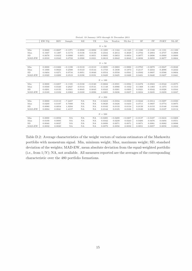
D.1 Analysis of weights
We also provide some summary statistics on the vectors of portfolio weights (w over time. In
each month, we compute the following four characteristics:
• Min: Minimum weight.
• Max: Maximum weight.
• SD: Standard deviation of weights.
• MAD-EW: Mean absolute deviation from equal-weighted portfolio computed as
1
N
N0
i=1
''' (wi −1
N
''' .
For each characteristic, we then report the average outcome over the 480 portfolio formations.
Table D.2 reports the results. Not surprisingly, the most dispersed weights are found for
Sample, followed by three shrinkage methods, EW-TQ, and BSV. The least dispersed weights
are always found for KZ and TZ, which is owed to the fact that these two portfolios are not
fully invested in the N stocks but also invest (generally to a large extent) in the risk-free rate.
NonLin and NL-Inv are comparably dispersed to Lin for N = 30, 50 but less dispersed than
Lin for N = 100, 250, 500.
There is no clear ordering among the four factor-based portfolios and the dispersion of their
weights is comparable to the rotation-equivariant shrinkage portfolios.
D.2 Robustness checks
The goal of this section is to examine whether the outperformance of NonLin over Lin is robust
to various changes in the empirical analysis.
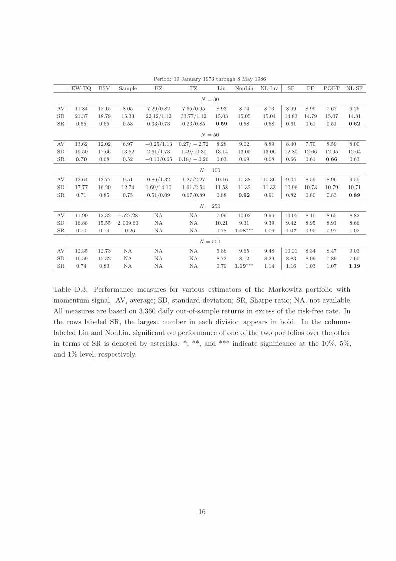
Subperiod analysis
The out-of-sample period comprises 480 months (or 10,080 days). It might be possible
that the outperformance of NonLin over Lin is driven by certain subperiods but does not hold
universally. We address this concern by dividing the out-of-sample period into three subperiods
of 160 months (or 3,360 days) each and repeating the above exercises in each subperiod.
Tables D.3–D.5 report the results. It can be seen that NonLin is better than Lin in terms
of the Sharpe ratio in 14 out of the 15 cases; though statistical significance only obtains in the
first subperiod for N = 250, 500.
Therefore, this analysis demonstrates that the outperformance of NonLin over Lin is
consistent over time and not due to a subperiod artifact. On balance, NonLin can be considered
equally as good as NL-SF.
9
Longer estimation window
Generally, at any investment date h, a covariance matrix is estimated using the most recent
T = 250 daily returns, corresponding roughly to one year of past data. As a robustness check,
we alternatively use the most recent T = 500 daily returns, corresponding roughly to two years
of past data.
Table D.6 reports the results, which are similar to the results in Table D.1. In particular,
NonLin has the uniformly best performance in terms of the Sharpe ratio, though the
outperformance over Lin is not statistically significant. Again, on balance, NonLin and NL-SF
are equally good.
Winsorization of past returns
Financial return data frequently contain unusually large (in absolute value) observations.
In order to mitigate the effect of such observations on an estimated covariance matrix, we
employ a winsorization technique, as is standard with quantitative portfolio managers; the
details can be found in Appendix C. Of course, we always use the actual, non-winsorized data
in computing the out-of-sample portfolio returns.
Table D.7 reports the results, which are similar to the results in Table D.1. In particular,
NonLin has the uniformly best performance among the rotation-equivariant portfolios in terms
of the Sharpe ratio, though the outperformance over Lin is not statistically significant. Again,
on balance, NonLin and NL-SF are equally good.
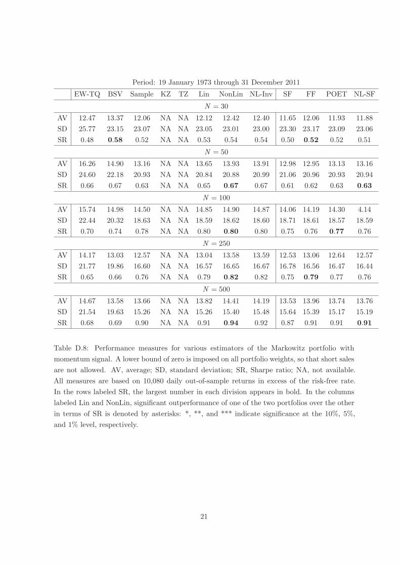
No-short-sales constraint
Since some fund managers face a no-short-sales constraint, we now impose a lower bound
of zero on all portfolio weights.
Table D.8 reports the results. Note that Sample is now available for all N , whereas KZ
and TZ are not available at all. In contrast to the previous results for the global mininum-
variance portfolio under a no-short-sales constraint in Section 4.5, improved estimation of the
covariance matrix still pays off, even if to a lesser extent compared to allowing short sales.
In particular — comparing the results for the rotation-equivariant portfolios — Lin, NonLin,
and NL-Inv improve upon Sample in terms of the Sharpe ratio for all N . Although BSV has
the best performance for N = 30, NonLin has the best performance for N = 50, 100, 250, 500.
In particular, NonLin always outperforms Lin, though no longer with statistical significance.
There is no clear winner among the factor-based portfolios: FF is best twice, POET is best
once, and NL-SF is best twice. (On the other hand, there is a clear loser, namely SF which is
always worst.) Overall, the factor-based portfolios have a somewhat worse performance than
the rotation-equivariant portfolios, which is in contrast to the results for the global minimum-
variance portfolio under a no-short-sales constraint in Section 4.5.
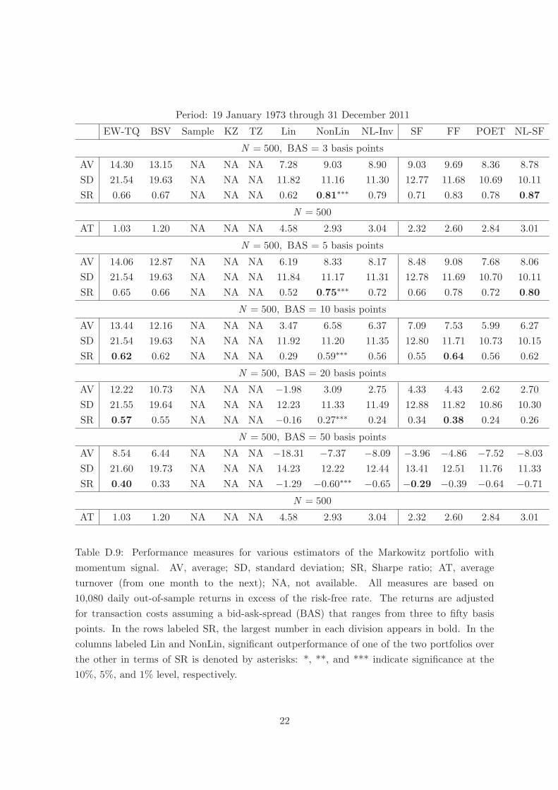
Transaction costs
Again, a detailed empirical study of real-life constrained portfolio selection that actively
limits portfolio turnover (and thus transaction costs) from one month to the next is beyond
the scope of the present paper.
10
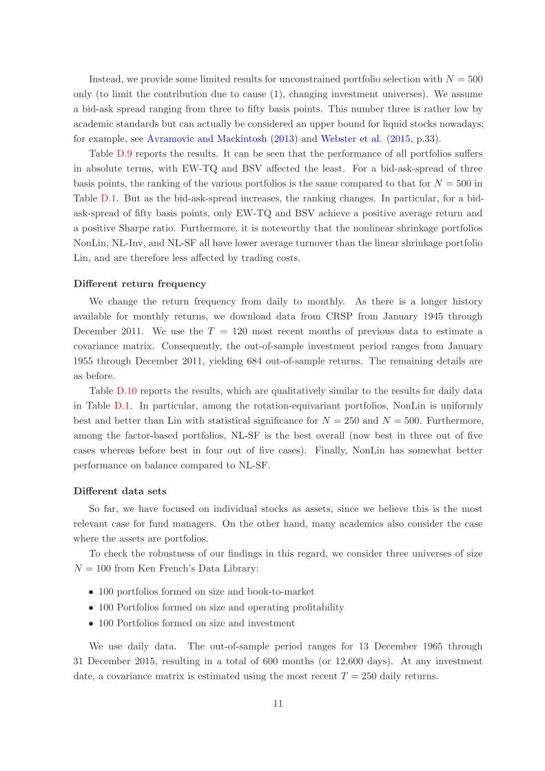
Instead, we provide some limited results for unconstrained portfolio selection with N = 500
only (to limit the contribution due to cause (1), changing investment universes). We assume
a bid-ask spread ranging from three to fifty basis points. This number three is rather low by
academic standards but can actually be considered an upper bound for liquid stocks nowadays;
for example, see Avramovic and Mackintosh (2013) and Webster et al. (2015, p.33).
Table D.9 reports the results. It can be seen that the performance of all portfolios suffers
in absolute terms, with EW-TQ and BSV affected the least. For a bid-ask-spread of three
basis points, the ranking of the various portfolios is the same compared to that for N = 500 in
Table D.1. But as the bid-ask-spread increases, the ranking changes. In particular, for a bid-
ask-spread of fifty basis points, only EW-TQ and BSV achieve a positive average return and
a positive Sharpe ratio. Furthermore, it is noteworthy that the nonlinear shrinkage portfolios
NonLin, NL-Inv, and NL-SF all have lower average turnover than the linear shrinkage portfolio
Lin, and are therefore less affected by trading costs.
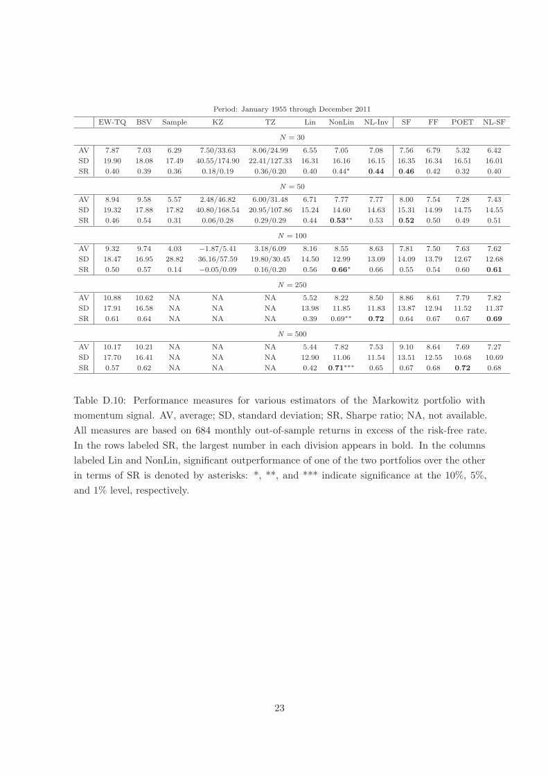
Different return frequency
We change the return frequency from daily to monthly. As there is a longer history
available for monthly returns, we download data from CRSP from January 1945 through
December 2011. We use the T = 120 most recent months of previous data to estimate a
covariance matrix. Consequently, the out-of-sample investment period ranges from January
1955 through December 2011, yielding 684 out-of-sample returns. The remaining details are
as before.
Table D.10 reports the results, which are qualitatively similar to the results for daily data
in Table D.1. In particular, among the rotation-equivariant portfolios, NonLin is uniformly
best and better than Lin with statistical significance for N = 250 and N = 500. Furthermore,
among the factor-based portfolios, NL-SF is the best overall (now best in three out of five
cases whereas before best in four out of five cases). Finally, NonLin has somewhat better
performance on balance compared to NL-SF.
Different data sets
So far, we have focused on individual stocks as assets, since we believe this is the most
relevant case for fund managers. On the other hand, many academics also consider the case
where the assets are portfolios.
To check the robustness of our findings in this regard, we consider three universes of size
N = 100 from Ken French’s Data Library:
• 100 portfolios formed on size and book-to-market
• 100 Portfolios formed on size and operating profitability
• 100 Portfolios formed on size and investment
We use daily data. The out-of-sample period ranges for 13 December 1965 through
31 December 2015, resulting in a total of 600 months (or 12,600 days). At any investment
date, a covariance matrix is estimated using the most recent T = 250 daily returns.
11

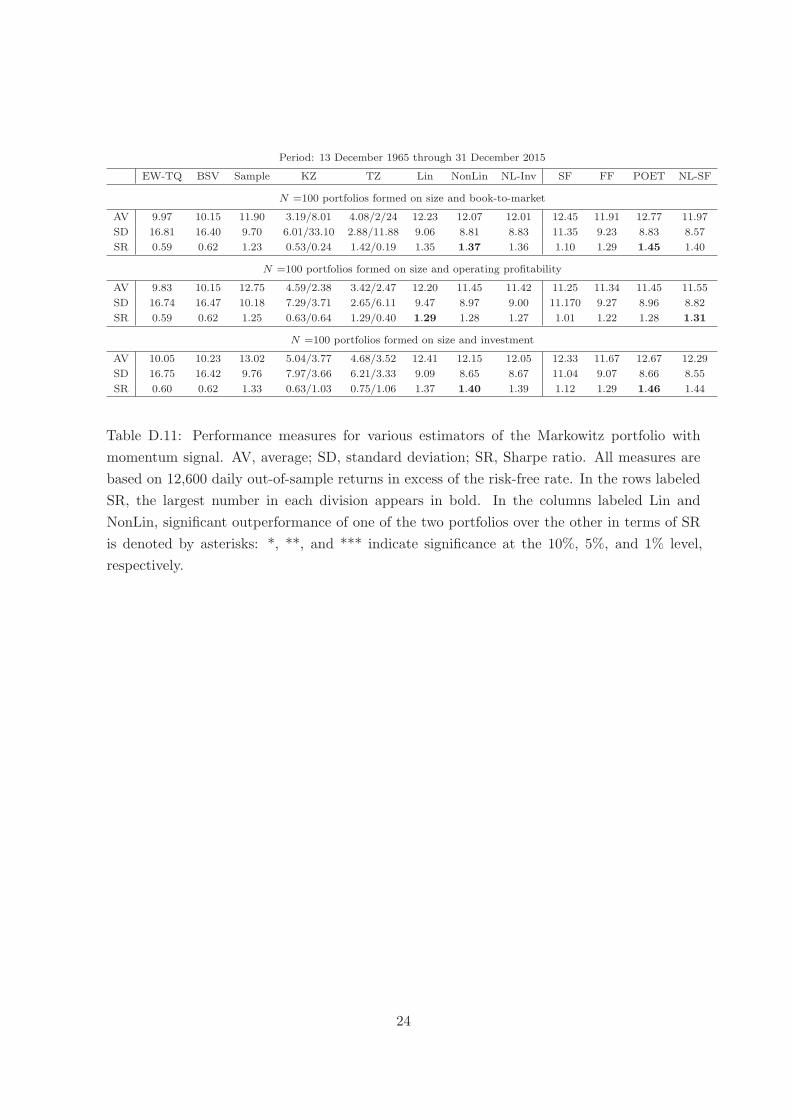
Table D.11 reports the results, which are similar to the results in Table D.1 in a relative
sense, though they are better in an absolute sense. Among the rotation-equivariant portfolios,
NonLin is best twice and Lin is best once (though the differences are not statistically significant).
Among the factor-based portfolios, POET is best twice and NL-SF is best once. Finally,
for these data sets, NL-SF is uniformly better than NonLin (though not with statistical
significance).
Remark D.3 (Optimal versus Naıve Diversification). DeMiguel et al. (2009) claim that it is
very difficult to outperform the naıve equal-weighted portfolio with sophisticated Markowitz
portfolios due to the estimation error in the inputs required by Markowitz portfolios; their
claim is concerning outperformance in terms of the Sharpe ratio and certainty equivalents.
In contrast, we find that shrinkage estimation of the covariance matrix combined with the
momentum signal results in consistently higher Sharpe ratios compared to the equal-weighted
portfolio.6 In particular, this outperformance also holds in the recent past, when the
momentum signal was not as strong anymore compared to the more distant past; see Tables 5
and D.5. This finding is encouraging to sophisticated investment managers: If they can come
up with a good signal and combine it with nonlinear shrinkage estimation of the covariance
matrix, outperforming the equal-weighted portfolio is far from a hopeless task.
D.3 Summary of results
We have carried out an extensive backtest analysis, evaluating the out-of-sample performance
of our nonlinear shrinkage estimator when used to estimate a full Markowitz portfolio with
momentum signal; in this setting, the primary performance criterion is the Sharpe ratio of
realized out-of-sample returns (in excess of the risk-free rate). We have compared nonlinear
shrinkage to a number of other strategies to estimate the global mininum-variance portfolio,
most of them proposed in the last decade in leading finance and econometrics journals. The
portfolios considered can be classified into rotation-equivariant portfolios and portfolios based
on factor models.
Our main analysis is based on daily data with an out-of-sample investment period ranging
from 1973 throughout 2011. We have added a large number of robustness checks to study the
sensitivity of our findings. Such robustness checks include a subsample analysis, changing the
length of the estimation window of past data to estimate a covariance matrix, winsorization
of past returns to estimate a covariance matrix, imposing a no-short-sales constraint, and
changing the return frequency from daily data to monthly data (where the beginning of the
out-of-sample investment period is moved back to 1955).
Among the rotation-equivariant portfolios, nonlinear shrinkage is the clear winner; in
particular, it consistently outperforms linear shrinkage. Among the factor-based portfolios,
6Of the many scenarios considered, there is a single one in which the equal-weighted portfolio has a higher
Sharpe ratio than linear shrinkage combined with the momentum signal, namely with monthly data for N = 30;
see Tables 10 and D.10. On the other hand, the equal-weighted portfolio always has a lower Sharpe ratio than
nonlinear shrinkage combined with the momentum signal.
12

applying nonlinear shrinkage after preconditioning the data using a single-factor model is the
overall the best. When comparing this hybrid method to linear shrinkage, there is no winner;
on balance, the two methods perform about equally well.
The statements of the previous paragraph only apply to unrestricted estimation of the
Markowitz portfolio when short sales (i.e., negative portfolio weights) are allowed. Consistent
with the findings of Jagannathan and Ma (2003), the relative performances change when short
sales are not allowed (i.e., when portfolio weights are constrained to be non-negative). In this
case, sophisticated portfolios still outperform the sample covariance matrix, though to a lesser
extent compared to unrestricted estimation. Moreover, nonlinear shrinkage is overall best,
outperforming all factor-based portfolios in particular.
13
Period: 19 January 1973 through 31 December 2011
EW-TQ BSV Sample KZ TZ Lin NonLin NL-Inv SF FF POET NL-SF
N = 30
AV 12.47 13.37 11.22 4.14/0.83 2.38/0.72 11.29 11.87 11.87 11.76 11.87 10.82 11.83
SD 25.77 23.15 18.86 16.31/1.58 19.64/1.84 18.58 18.57 18.57 18.76 18.47 18.80 18.16
SR 0.48 0.58 0.60 0.25/0.52 0.12/0.39 0.61 0.64 0.64 0.48 0.64 0.58 0.65
N = 50
AV 16.26 14.90 10.32 0.13/− 0.02 0.50/− 0.89 11.70 12.12 12.04 11.08 11.35 10.77 11.43
SD 24.60 22.18 16.86 2.66/8.83 2.25/6.57 16.30 16.23 16.24 16.34 15.99 16.15 15.80
SR 0.66 0.67 0.61 0.05/− 0.07 −0.00/− 0.14 0.72 0.75 0.74 0.68 0.71 0.67 0.72
N = 100
AV 15.74 14.98 10.93 −4.70/− 0.56 1.23/1.88 11.97 12.31 12.31 10.67 11.86 10.66 11.00
SD 22.44 20.32 16.00 25.34/15.41 1.85/2.48 14.68 14.30 14.30 14.68 14.16 14.04 13.82
SR 0.70 0.74 0.68 −0.19/− 0.04 0.66/0.76 0.82 0.86 0.86 0.73 0.84 0.76 0.80
N = 250
AV 14.17 13.03 275.01 NA NA 10.04 11.12 11.38 10.80 11.45 10.32 10.36
SD 21.77 19.86 3, 542.92 NA NA 12.82 12.14 12.32 13.20 12.33 11.74 11.26
SR 0.65 0.66 0.08 NA NA 0.78 0.92∗∗ 0.92 0.82 0.93 0.88 0.92
N = 500
AV 14.67 13.58 NA NA NA 8.92 9.94 9.87 9.86 10.62 9.37 9.85
SD 21.54 19.63 NA NA NA 11.82 11.09 11.26 12.77 11.68 10.69 10.10
SR 0.68 0.69 NA NA NA 0.75 0.90∗∗ 0.88 0.77 0.91 0.88 0.97
Table D.1: Performance measures for various estimators of the Markowitz portfolio with
momentum signal. AV, average; SD, standard deviation; SR, Sharpe ratio; NA, not available.
All measures are based on 10,080 daily out-of-sample returns in excess of the risk-free rate.
In the rows labeled SR, the largest number in each division appears in bold. In the columns
labeled Lin and NonLin, significant outperformance of one of the two portfolios over the other
in terms of SR is denoted by asterisks: *, **, and *** indicate significance at the 10%, 5%,
and 1% level, respectively.
14
Period: 19 January 1973 through 31 December 2011
EW-TQ BSV Sample KZ TZ Lin NonLin NL-Inv SF FF POET NL-SF
N = 50
Min 0.0000 −0.0687 −0.1371 −0.0098 −0.0092 −0.1095 −0.1164 −0.1165 −0.1026 −0.1108 −0.1191 −0.1109
Max 0.1667 0.1287 0.3173 0.0136 0.0139 0.2344 0.2612 0.2629 0.2792 0.2904 0.2757 0.2908
SD 0.0678 0.0452 0.0988 0.0051 0.0051 0.0805 0.0853 0.0854 0.0877 0.0896 0.0900 0.0899
MAD-EW 0.0533 0.0343 0.0722 0.0326 0.0321 0.0618 0.0642 0.0642 0.0656 0.0659 0.0677 0.0664
N = 50
Min 0.0000 −0.0466 −0.1198 −0.0118 −0.0110 −0.0895 −0.0883 −0.0886 −0.0763 −0.0879 −0.0847 −0.0848
Max 0.1000 0.0823 0.2588 0.0143 0.0144 0.1733 0.1838 0.1873 0.2117 0.2244 0.2088 0.2242
SD 0.0404 0.0271 0.0716 0.0051 0.0049 0.0554 0.0558 0.0561 0.0582 0.0607 0.0588 0.0604
MAD-EW 0.0320 0.0206 0.0519 0.0196 0.0191 0.0428 0.0425 0.0426 0.0431 0.0440 0.0437 0.0441
N = 100
Min 0.0000 −0.0257 −0.1105 −0.0130 −0.0120 −0.0682 −0.0591 −0.0594 −0.0478 −0.0583 −0.0542 −0.0575
Max 0.0500 0.0446 0.2027 0.0144 0.0141 0.1148 0.0986 0.1032 0.1368 0.1483 0.1373 0.1515
SD 0.0201 0.0135 0.0501 0.0045 0.0043 0.0343 0.0301 0.0305 0.0321 0.0342 0.0326 0.0344
MAD-EW 0.0160 0.0102 0.0362 0.0100 0.0096 0.0265 0.0236 0.0237 0.0234 0.0245 0.0239 0.0247
N = 250
Min 0.0000 −0.0110 −7.2457 NA NA −0.0452 −0.0334 −0.0338 −0.0242 −0.0314 −0.0297 −0.0330
Max 0.0200 0.0187 6.7088 NA NA 0.0620 0.0426 0.0433 0.0711 0.0807 0.0774 0.0875
SD 0.0080 0.0054 1.9294 NA NA 0.0182 0.0133 0.0134 0.0139 0.0153 0.0148 0.0160
MAD-EW 0.0064 0.0041 1.4157 NA NA 0.0144 0.0105 0.0106 0.0100 0.0108 0.0107 0.0114
N = 500
Min 0.0000 −0.0056 NA NA NA −0.0285 −0.0209 −0.0207 −0.0137 −0.0187 −0.0216 −0.0208
Max 0.0100 0.0095 NA NA NA 0.0342 0.0239 0.0243 0.0406 0.0476 0.0494 0.0551
SD 0.0040 0.0027 NA NA NA 0.0099 0.0071 0.0071 0.0071 0.0081 0.0082 0.0088
MAD-EW 0.0032 0.0020 NA NA NA 0.0079 0.0056 0.0056 0.0051 0.0057 0.0058 0.0062
Table D.2: Average characteristics of the weight vectors of various estimators of the Markowitz
portfolio with momentum signal. Min, mininum weight; Max, maximum weight; SD, standard
deviation of the weights; MAD-EW, mean absolute deviation from the equal-weighted portfolio
(i.e., from 1/N); NA, not available. All measures reported are the averages of the corresponding
characteristic over the 480 portfolio formations.
15
Period: 19 January 1973 through 8 May 1986
EW-TQ BSV Sample KZ TZ Lin NonLin NL-Inv SF FF POET NL-SF
N = 30
AV 11.84 12.15 8.05 7.29/0.82 7.65/0.95 8.93 8.74 8.73 8.99 8.99 7.67 9.25
SD 21.37 18.79 15.33 22.12/1.12 33.77/1.12 15.03 15.05 15.04 14.83 14.79 15.07 14.81
SR 0.55 0.65 0.53 0.33/0.73 0.23/0.85 0.59 0.58 0.58 0.61 0.61 0.51 0.62
N = 50
AV 13.62 12.02 6.97 −0.25/1.13 0.27/− 2.72 8.28 9.02 8.89 8.40 7.70 8.59 8.00
SD 19.50 17.66 13.52 2.61/1.73 1.49/10.30 13.14 13.05 13.06 12.80 12.66 12.95 12.64
SR 0.70 0.68 0.52 −0.10/0.65 0.18/− 0.26 0.63 0.69 0.68 0.66 0.61 0.66 0.63
N = 100
AV 12.64 13.77 9.51 0.86/1.32 1.27/2.27 10.16 10.38 10.36 9.04 8.59 8.96 9.55
SD 17.77 16.20 12.74 1.69/14.10 1.91/2.54 11.58 11.32 11.33 10.96 10.73 10.79 10.71
SR 0.71 0.85 0.75 0.51/0.09 0.67/0.89 0.88 0.92 0.91 0.82 0.80 0.83 0.89
N = 250
AV 11.90 12.32 −527.28 NA NA 7.99 10.02 9.96 10.05 8.10 8.65 8.82
SD 16.88 15.55 2, 009.60 NA NA 10.21 9.31 9.39 9.42 8.95 8.91 8.66
SR 0.70 0.79 −0.26 NA NA 0.78 1.08∗∗∗ 1.06 1.07 0.90 0.97 1.02
N = 500
AV 12.35 12.73 NA NA NA 6.86 9.65 9.48 10.21 8.34 8.47 9.03
SD 16.59 15.32 NA NA NA 8.73 8.12 8.29 8.83 8.09 7.89 7.60
SR 0.74 0.83 NA NA NA 0.79 1.19∗∗∗ 1.14 1.16 1.03 1.07 1.19
Table D.3: Performance measures for various estimators of the Markowitz portfolio with
momentum signal. AV, average; SD, standard deviation; SR, Sharpe ratio; NA, not available.
All measures are based on 3,360 daily out-of-sample returns in excess of the risk-free rate. In
the rows labeled SR, the largest number in each division appears in bold. In the columns
labeled Lin and NonLin, significant outperformance of one of the two portfolios over the other
in terms of SR is denoted by asterisks: *, **, and *** indicate significance at the 10%, 5%,
and 1% level, respectively.
16

Period: 9 May 1986 through 25 August 1999
EW-TQ BSV Sample KZ TZ Lin NonLin NL-Inv SF FF POET NL-SF
N = 30
AV 14.06 11.89 12.27 −1.04/0.64 0.56/1.17 12.21 12.36 12.36 12.18 10.67 11.61 11.84
SD 23.70 21.94 19.13 3.66/1.34 1.29/2.44 18.68 18.55 18.55 18.42 18.48 19.00 18.19
SR 0.59 0.54 0.64 −0.28/0.48 0.43/0.48 0.65 0.67 0.67 0.66 0.58 0.61 0.65
N = 50
AV 19.81 18.06 10.08 0.70/0.48 1.47/0.01 11.46 11.74 11.73 10.82 11.29 10.31 11.40
SD 22.96 20.48 16.65 1.36/1.38 2.84/3.91 16.19 16.16 16.17 16.01 15.92 15.97 15.71
SR 0.86 0.88 0.61 0.52/0.34 0.52/0.00 0.71 0.73 0.73 0.68 0.71 0.65 0.73
N = 100
AV 20.25 18.20 12.63 0.64/2.44 1.34/2.19 13.20 14.00 14.07 9.79 11.48 11.06 11.65
SD 20.42 18.33 15.59 2.91/3.35 1.97/2.76 14.38 14.30 14.28 14.64 14.36 14.20 13.92
SR 0.99 0.99 0.81 0.22/0.73 0.68/0.79 0.92 0.98 0.99 0.67 0.80 0.78 0.84
N = 250
AV 18.12 15.08 652.50 NA NA 11.74 12.44 12.51 9.48 11.38 10.61 12.55
SD 19.57 17.78 2127.18 NA NA 11.95 11.86 12.01 12.24 11.65 11.60 11.00
SR 0.93 0.85 0.31 NA NA 0.98 1.05 1.04 0.78 0.98 0.91 1.14
N = 500
AV 18.95 16.35 NA NA NA 12.19 12.67 12.71 8.53 10.95 10.54 12.23
SD 19.39 17.62 NA NA NA 11.05 10.82 11.03 11.65 10.75 10.37 9.82
SR 0.98 0.93 NA NA NA 1.10 1.17 1.15 0.73 1.02 1.02 1.24
Table D.4: Performance measures for various estimators of the Markowitz portfolio with
momentum signal. AV, average; SD, standard deviation; SR, Sharpe ratio; NA, not available.
All measures are based on 3,360 daily out-of-sample returns in excess of the risk-free rate. In
the rows labeled SR, the largest number in each division appears in bold. In the columns
labeled Lin and NonLin, significant outperformance of one of the two portfolios over the other
in terms of SR is denoted by asterisks: *, **, and *** indicate significance at the 10%, 5%,
and 1% level, respectively.
17
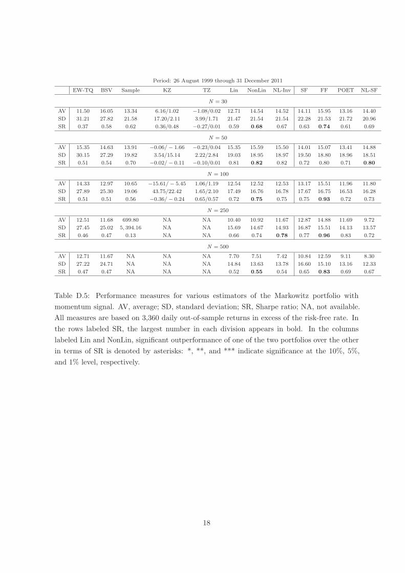
Period: 26 August 1999 through 31 December 2011
EW-TQ BSV Sample KZ TZ Lin NonLin NL-Inv SF FF POET NL-SF
N = 30
AV 11.50 16.05 13.34 6.16/1.02 −1.08/0.02 12.71 14.54 14.52 14.11 15.95 13.16 14.40
SD 31.21 27.82 21.58 17.20/2.11 3.99/1.71 21.47 21.54 21.54 22.28 21.53 21.72 20.96
SR 0.37 0.58 0.62 0.36/0.48 −0.27/0.01 0.59 0.68 0.67 0.63 0.74 0.61 0.69
N = 50
AV 15.35 14.63 13.91 −0.06/− 1.66 −0.23/0.04 15.35 15.59 15.50 14.01 15.07 13.41 14.88
SD 30.15 27.29 19.82 3.54/15.14 2.22/2.84 19.03 18.95 18.97 19.50 18.80 18.96 18.51
SR 0.51 0.54 0.70 −0.02/− 0.11 −0.10/0.01 0.81 0.82 0.82 0.72 0.80 0.71 0.80
N = 100
AV 14.33 12.97 10.65 −15.61/− 5.45 1.06/1.19 12.54 12.52 12.53 13.17 15.51 11.96 11.80
SD 27.89 25.30 19.06 43.75/22.42 1.65/2.10 17.49 16.76 16.78 17.67 16.75 16.53 16.28
SR 0.51 0.51 0.56 −0.36/− 0.24 0.65/0.57 0.72 0.75 0.75 0.75 0.93 0.72 0.73
N = 250
AV 12.51 11.68 699.80 NA NA 10.40 10.92 11.67 12.87 14.88 11.69 9.72
SD 27.45 25.02 5, 394.16 NA NA 15.69 14.67 14.93 16.87 15.51 14.13 13.57
SR 0.46 0.47 0.13 NA NA 0.66 0.74 0.78 0.77 0.96 0.83 0.72
N = 500
AV 12.71 11.67 NA NA NA 7.70 7.51 7.42 10.84 12.59 9.11 8.30
SD 27.22 24.71 NA NA NA 14.84 13.63 13.78 16.60 15.10 13.16 12.33
SR 0.47 0.47 NA NA NA 0.52 0.55 0.54 0.65 0.83 0.69 0.67
Table D.5: Performance measures for various estimators of the Markowitz portfolio with
momentum signal. AV, average; SD, standard deviation; SR, Sharpe ratio; NA, not available.
All measures are based on 3,360 daily out-of-sample returns in excess of the risk-free rate. In
the rows labeled SR, the largest number in each division appears in bold. In the columns
labeled Lin and NonLin, significant outperformance of one of the two portfolios over the other
in terms of SR is denoted by asterisks: *, **, and *** indicate significance at the 10%, 5%,
and 1% level, respectively.
18

Period: 19 January 1973 through 31 December 2011
EW-TQ BSV Sample KZ TZ Lin NonLin NL-Inv SF FF POET NL-SF
N = 30
AV 12.47 13.37 11.32 0.29/0.52 0.15/− 0.42 11.51 11.55 11.54 11.88 12.06 10.81 11.68
SD 25.77 23.15 18.44 0.93/2.61 1.22/5.76 18.32 18.33 18.33 18.90 18.51 18.76 18.25
SR 0.48 0.58 0.61 0.31/0.20 0.13/− 0.07 0.63 0.63 0.63 0.63 0.65 0.58 0.64
N = 50
AV 16.26 14.90 11.58 1.91/1.18 2.23/− 51.96 12.17 12.38 12.35 11.24 11.69 10.96 11.77
SD 24.60 22.18 16.25 7.52/3.12 10.80/326.59 16.12 16.11 16.11 16.50 16.16 16.31 15.91
SR 0.66 0.67 0.71 0.25/0.38 0.21/− 0.16 0.76 0.77 0.77 0.68 0.72 0.67 0.74
N = 100
AV 15.74 14.98 11.07 0.53/− 3.97 4.11/0.34 11.88 11.77 11.75 11.58 12.45 11.24 11.28
SD 22.44 20.32 14.54 2.29/26.46 22.56/5.34 14.15 14.03 14.04 14.62 14.15 13.86 13.64
SR 0.70 0.74 0.76 0.23/− 0.15 0.18/0.06 0.84 0.84 0.84 0.79 0.88 0.81 0.83
N = 250
AV 14.17 13.03 11.25 3.28/− 4.26 0.60/− 2.04 10.72 11.05 11.16 11.27 11.54 9.87 10.64
SD 21.77 19.86 13.70 9.44/30.63 5.76/42.38 12.26 11.85 11.88 13.41 12.66 11.82 11.28
SR 0.65 0.66 0.82 0.35/− 0.14 0.10/− 0.05 0.87 0.93 0.94 0.84 0.91 0.83 0.94
N = 500
AV 14.67 13.58 1, 205.18 NA NA 10.53 10.57 10.55 10.52 10.97 9.51 10.36
SD 21.54 19.63 8, 551.62 NA NA 11.95 10.89 11.33 12.99 12.11 10.77 10.09
SR 0.68 0.69 0.14 NA NA 0.88 0.97 0.93 0.81 0.91 0.88 1.03
Table D.6: Performance measures for various estimators of the Markowitz portfolio with
momentum signal. The past window to estimate the covariance matrix is taken to be of
length T = 500 days instead of T = 250 days. AV, average; SD, standard deviation; SR,
Sharpe ratio; NA, not available. All measures are based on 10,080 daily out-of-sample returns
in excess of the risk-free rate. In the rows labeled SR, the largest number in each division
appears in bold. In the columns labeled Lin and NonLin, significant outperformance of one of
the two portfolios over the other in terms of SR is denoted by asterisks: *, **, and *** indicate
significance at the 10%, 5%, and 1% level, respectively.
19

Period: 19 January 1973 through 31 December 2011
EW-TQ BSV Sample KZ TZ Lin NonLin NL-Inv SF FF POET NL-SF
N = 30
AV 12.47 13.37 11.27 0.82/− 0.54 2.08/0.59 11.38 11.87 11.89 11.89 12.23 12.19 11.99
SD 25.77 23.15 19.16 3.61/3.67 4.68/3.02 18.83 18.77 18.77 19.06 18.66 19.28 18.46
SR 0.48 0.58 0.59 0.23/− 0.15 0.45/0.19 0.60 0.63 0.63 0.62 0.66 0.63 0.65
N = 50
AV 16.26 14.90 10.71 1.62/2.54 −5.88/− 2.19 11.46 12.11 12.04 11.30 11.68 10.24 11.69
SD 24.60 22.18 17.12 8.05/7.80 32.69/18.76 16.65 16.55 16.55 16.61 16.10 16.54 15.97
SR 0.66 0.67 0.63 0.20/0.33 −0.18/− 0.12 0.69 0.73 0.73 0.68 0.73 0.62 0.73
N = 100
AV 15.74 14.98 10.47 0.52/− 0.98 1.12/2.72 11.39 11.81 11.78 10.84 12.07 10.07 10.75
SD 22.44 20.32 16.39 18.21/15.78 6.16/16.12 15.05 14.74 14.70 14.93 14.24 14.29 13.98
SR 0.70 0.74 0.64 0.03/− 0.06 0.18/0.18 0.76 0.80 0.80 0.73 0.85 0.70 0.77
N = 250
AV 14.17 13.03 −2, 498.52 NA NA 10.70 11.36 11.37 10.87 11.67 10.24 10.56
SD 21.77 19.86 12, 130.23 NA NA 13.82 12.46 12.48 13.38 12.38 11.56 11.35
SR 0.65 0.66 −0.21 NA NA 0.77 0.91∗ 0.91 0.81 0.94 0.89 0.93
N = 500
AV 14.67 13.58 NA NA NA 9.16 10.43 10.35 10.05 10.99 9.76 10.16
SD 21.54 19.63 NA NA NA 12.59 11.33 11.45 12.91 11.69 10.28 10.16
SR 0.68 0.69 NA NA NA 0.73 0.92∗∗ 0.90 0.78 0.94 0.95 1.00
Table D.7: Performance measures for various estimators of the Markowitz portfolio with
momentum signal. In the estimation of a covariance matrix, the past returns are winsorized
as described in Appendix C. AV, average; SD, standard deviation; SR, Sharpe ratio; NA, not
available. All measures are based on 10,080 daily out-of-sample returns in excess of the risk-
free rate. In the rows labeled SR, the largest number in each division appears in bold. In the
columns labeled Lin and NonLin, significant outperformance of one of the two portfolios over
the other in terms of SR is denoted by asterisks: *, **, and *** indicate significance at the
10%, 5%, and 1% level, respectively.
20
Period: 19 January 1973 through 31 December 2011
EW-TQ BSV Sample KZ TZ Lin NonLin NL-Inv SF FF POET NL-SF
N = 30
AV 12.47 13.37 12.06 NA NA 12.12 12.42 12.40 11.65 12.06 11.93 11.88
SD 25.77 23.15 23.07 NA NA 23.05 23.01 23.00 23.30 23.17 23.09 23.06
SR 0.48 0.58 0.52 NA NA 0.53 0.54 0.54 0.50 0.52 0.52 0.51
N = 50
AV 16.26 14.90 13.16 NA NA 13.65 13.93 13.91 12.98 12.95 13.13 13.16
SD 24.60 22.18 20.93 NA NA 20.84 20.88 20.99 21.06 20.96 20.93 20.94
SR 0.66 0.67 0.63 NA NA 0.65 0.67 0.67 0.61 0.62 0.63 0.63
N = 100
AV 15.74 14.98 14.50 NA NA 14.85 14.90 14.87 14.06 14.19 14.30 4.14
SD 22.44 20.32 18.63 NA NA 18.59 18.62 18.60 18.71 18.61 18.57 18.59
SR 0.70 0.74 0.78 NA NA 0.80 0.80 0.80 0.75 0.76 0.77 0.76
N = 250
AV 14.17 13.03 12.57 NA NA 13.04 13.58 13.59 12.53 13.06 12.64 12.57
SD 21.77 19.86 16.60 NA NA 16.57 16.65 16.67 16.78 16.56 16.47 16.44
SR 0.65 0.66 0.76 NA NA 0.79 0.82 0.82 0.75 0.79 0.77 0.76
N = 500
AV 14.67 13.58 13.66 NA NA 13.82 14.41 14.19 13.53 13.96 13.74 13.76
SD 21.54 19.63 15.26 NA NA 15.26 15.40 15.48 15.64 15.39 15.17 15.19
SR 0.68 0.69 0.90 NA NA 0.91 0.94 0.92 0.87 0.91 0.91 0.91
Table D.8: Performance measures for various estimators of the Markowitz portfolio with
momentum signal. A lower bound of zero is imposed on all portfolio weights, so that short sales
are not allowed. AV, average; SD, standard deviation; SR, Sharpe ratio; NA, not available.
All measures are based on 10,080 daily out-of-sample returns in excess of the risk-free rate.
In the rows labeled SR, the largest number in each division appears in bold. In the columns
labeled Lin and NonLin, significant outperformance of one of the two portfolios over the other
in terms of SR is denoted by asterisks: *, **, and *** indicate significance at the 10%, 5%,
and 1% level, respectively.
21
Period: 19 January 1973 through 31 December 2011
EW-TQ BSV Sample KZ TZ Lin NonLin NL-Inv SF FF POET NL-SF
N = 500, BAS = 3 basis points
AV 14.30 13.15 NA NA NA 7.28 9.03 8.90 9.03 9.69 8.36 8.78
SD 21.54 19.63 NA NA NA 11.82 11.16 11.30 12.77 11.68 10.69 10.11
SR 0.66 0.67 NA NA NA 0.62 0.81∗∗∗ 0.79 0.71 0.83 0.78 0.87
N = 500
AT 1.03 1.20 NA NA NA 4.58 2.93 3.04 2.32 2.60 2.84 3.01
N = 500, BAS = 5 basis points
AV 14.06 12.87 NA NA NA 6.19 8.33 8.17 8.48 9.08 7.68 8.06
SD 21.54 19.63 NA NA NA 11.84 11.17 11.31 12.78 11.69 10.70 10.11
SR 0.65 0.66 NA NA NA 0.52 0.75∗∗∗ 0.72 0.66 0.78 0.72 0.80
N = 500, BAS = 10 basis points
AV 13.44 12.16 NA NA NA 3.47 6.58 6.37 7.09 7.53 5.99 6.27
SD 21.54 19.63 NA NA NA 11.92 11.20 11.35 12.80 11.71 10.73 10.15
SR 0.62 0.62 NA NA NA 0.29 0.59∗∗∗ 0.56 0.55 0.64 0.56 0.62
N = 500, BAS = 20 basis points
AV 12.22 10.73 NA NA NA −1.98 3.09 2.75 4.33 4.43 2.62 2.70
SD 21.55 19.64 NA NA NA 12.23 11.33 11.49 12.88 11.82 10.86 10.30
SR 0.57 0.55 NA NA NA −0.16 0.27∗∗∗ 0.24 0.34 0.38 0.24 0.26
N = 500, BAS = 50 basis points
AV 8.54 6.44 NA NA NA −18.31 −7.37 −8.09 −3.96 −4.86 −7.52 −8.03
SD 21.60 19.73 NA NA NA 14.23 12.22 12.44 13.41 12.51 11.76 11.33
SR 0.40 0.33 NA NA NA −1.29 −0.60∗∗∗ −0.65 −0.29 −0.39 −0.64 −0.71
N = 500
AT 1.03 1.20 NA NA NA 4.58 2.93 3.04 2.32 2.60 2.84 3.01
Table D.9: Performance measures for various estimators of the Markowitz portfolio with
momentum signal. AV, average; SD, standard deviation; SR, Sharpe ratio; AT, average
turnover (from one month to the next); NA, not available. All measures are based on
10,080 daily out-of-sample returns in excess of the risk-free rate. The returns are adjusted
for transaction costs assuming a bid-ask-spread (BAS) that ranges from three to fifty basis
points. In the rows labeled SR, the largest number in each division appears in bold. In the
columns labeled Lin and NonLin, significant outperformance of one of the two portfolios over
the other in terms of SR is denoted by asterisks: *, **, and *** indicate significance at the
10%, 5%, and 1% level, respectively.
22
Period: January 1955 through December 2011
EW-TQ BSV Sample KZ TZ Lin NonLin NL-Inv SF FF POET NL-SF
N = 30
AV 7.87 7.03 6.29 7.50/33.63 8.06/24.99 6.55 7.05 7.08 7.56 6.79 5.32 6.42
SD 19.90 18.08 17.49 40.55/174.90 22.41/127.33 16.31 16.16 16.15 16.35 16.34 16.51 16.01
SR 0.40 0.39 0.36 0.18/0.19 0.36/0.20 0.40 0.44∗ 0.44 0.46 0.42 0.32 0.40
N = 50
AV 8.94 9.58 5.57 2.48/46.82 6.00/31.48 6.71 7.77 7.77 8.00 7.54 7.28 7.43
SD 19.32 17.88 17.82 40.80/168.54 20.95/107.86 15.24 14.60 14.63 15.31 14.99 14.75 14.55
SR 0.46 0.54 0.31 0.06/0.28 0.29/0.29 0.44 0.53∗∗ 0.53 0.52 0.50 0.49 0.51
N = 100
AV 9.32 9.74 4.03 −1.87/5.41 3.18/6.09 8.16 8.55 8.63 7.81 7.50 7.63 7.62
SD 18.47 16.95 28.82 36.16/57.59 19.80/30.45 14.50 12.99 13.09 14.09 13.79 12.67 12.68
SR 0.50 0.57 0.14 −0.05/0.09 0.16/0.20 0.56 0.66∗ 0.66 0.55 0.54 0.60 0.61
N = 250
AV 10.88 10.62 NA NA NA 5.52 8.22 8.50 8.86 8.61 7.79 7.82
SD 17.91 16.58 NA NA NA 13.98 11.85 11.83 13.87 12.94 11.52 11.37
SR 0.61 0.64 NA NA NA 0.39 0.69∗∗ 0.72 0.64 0.67 0.67 0.69
N = 500
AV 10.17 10.21 NA NA NA 5.44 7.82 7.53 9.10 8.64 7.69 7.27
SD 17.70 16.41 NA NA NA 12.90 11.06 11.54 13.51 12.55 10.68 10.69
SR 0.57 0.62 NA NA NA 0.42 0.71∗∗∗ 0.65 0.67 0.68 0.72 0.68
Table D.10: Performance measures for various estimators of the Markowitz portfolio with
momentum signal. AV, average; SD, standard deviation; SR, Sharpe ratio; NA, not available.
All measures are based on 684 monthly out-of-sample returns in excess of the risk-free rate.
In the rows labeled SR, the largest number in each division appears in bold. In the columns
labeled Lin and NonLin, significant outperformance of one of the two portfolios over the other
in terms of SR is denoted by asterisks: *, **, and *** indicate significance at the 10%, 5%,
and 1% level, respectively.
23
Period: 13 December 1965 through 31 December 2015
EW-TQ BSV Sample KZ TZ Lin NonLin NL-Inv SF FF POET NL-SF
N =100 portfolios formed on size and book-to-market
AV 9.97 10.15 11.90 3.19/8.01 4.08/2/24 12.23 12.07 12.01 12.45 11.91 12.77 11.97
SD 16.81 16.40 9.70 6.01/33.10 2.88/11.88 9.06 8.81 8.83 11.35 9.23 8.83 8.57
SR 0.59 0.62 1.23 0.53/0.24 1.42/0.19 1.35 1.37 1.36 1.10 1.29 1.45 1.40
N =100 portfolios formed on size and operating profitability
AV 9.83 10.15 12.75 4.59/2.38 3.42/2.47 12.20 11.45 11.42 11.25 11.34 11.45 11.55
SD 16.74 16.47 10.18 7.29/3.71 2.65/6.11 9.47 8.97 9.00 11.170 9.27 8.96 8.82
SR 0.59 0.62 1.25 0.63/0.64 1.29/0.40 1.29 1.28 1.27 1.01 1.22 1.28 1.31
N =100 portfolios formed on size and investment
AV 10.05 10.23 13.02 5.04/3.77 4.68/3.52 12.41 12.15 12.05 12.33 11.67 12.67 12.29
SD 16.75 16.42 9.76 7.97/3.66 6.21/3.33 9.09 8.65 8.67 11.04 9.07 8.66 8.55
SR 0.60 0.62 1.33 0.63/1.03 0.75/1.06 1.37 1.40 1.39 1.12 1.29 1.46 1.44
Table D.11: Performance measures for various estimators of the Markowitz portfolio with
momentum signal. AV, average; SD, standard deviation; SR, Sharpe ratio. All measures are
based on 12,600 daily out-of-sample returns in excess of the risk-free rate. In the rows labeled
SR, the largest number in each division appears in bold. In the columns labeled Lin and
NonLin, significant outperformance of one of the two portfolios over the other in terms of SR
is denoted by asterisks: *, **, and *** indicate significance at the 10%, 5%, and 1% level,
respectively.
24
References
Avramovic, A. and P. Mackintosh (2013, May). Inside the NBBO: Pushing for wider — and
narrower! — spreads. Trading strategy: Market commentary, Credit Suisse Research and
Analytics, New York, USA.
Bai, Z. D. and J. W. Silverstein (2010). Spectral Analysis of Large-Dimensional Random
Matrices (Second ed.). New York: Springer.
Brandt, M. W., P. Santa-Clara, and R. Valkanov (2009). Parametric portfolio policies:
Exploiting characteristics in the cross-section of equity returns. Review of Financial
Studies 22 (9), 3411–3447.
Chincarini, L. B. and D. Kim (2006). Quantitative Equity Portfolio Management: An Active
Approach to Portfolio Construction and Management. New York: McGraw-Hill.
DeMiguel, V., L. Garlappi, and R. Uppal (2009). Optimal versus naive diversification: How
inefficient is the 1/N portfolio strategy? Review of Financial Studies 22, 1915–1953.
Fama, E. F. and K. R. French (1993). Common risk factors in the returns on stocks and bonds.
Journal of Financial Economics 33 (1), 3–56.
Fan, J., Y. Liao, and M. Mincheva (2013). Large covariance estimation by thresholding
principal orthogonal complements (with discussion). Journal of the Royal Statistical Society,
Series B 75 (4), 603–680.
Huang, C. and R. Litzenberger (1988). Foundations for Financial Economics. New York:
North-Holland.
Jagannathan, R. and T. Ma (2003). Risk reduction in large portfolios: Why imposing the
wrong constraints helps. Journal of Finance 54 (4), 1651–1684.
Jegadeesh, N. and S. Titman (1993). Returns to buying winners and selling losers: Implications
for stock market efficiency. Journal of Finance 48 (1), 65–91.
Kan, R. and G. Zhou (2007). Optimal portfolio choice with parameter uncertainty. Journal
of Financial and Quantitative Analysis 42 (3), 621–656.
Ledoit, O. and S. Peche (2011). Eigenvectors of some large sample covariance matrix ensembles.
Probability Theory and Related Fields 150 (1–2), 233–264.
Ledoit, O. and M. Wolf (2004). A well-conditioned estimator for large-dimensional covariance
matrices. Journal of Multivariate Analysis 88 (2), 365–411.
Ledoit, O. and M. Wolf (2008). Robust performance hypothesis testing with the Sharpe ratio.
Journal of Empirical Finance 15, 850–859.
25

Ledoit, O. and M. Wolf (2012). Nonlinear shrinkage estimation of large-dimensional covariance
matrices. Annals of Statistics 40 (2), 1024–1060.
Ledoit, O. and M. Wolf (2015). Spectrum estimation: a unified framework for covariance
matrix estimation and PCA in large dimensions. Journal of Multivariate Analysis 139 (2),
360–384.
Ledoit, O. and M. Wolf (2018). Optimal estimation of a large-dimensional covariance matrix
under Stein’s loss. Bernoulli . Forthcoming.
Tu, J. and G. Zhou (2011). Markowitz meets Talmud: A combination of sophisticated and
naive diversification strategies. Journal of Financial Economics 99 (1), 204–215.
Webster, K., Y. Luo, M.-A. Alvarez, J. Jussa, S. Wang, G. Rohal, A. Wang, D. Elledge, and
G. Zhao (2015, July). A portfolio manager’s guidebook to trade execution: From light rays
to dark pools. Quantitative strategy: Signal processing, Deutsche Bank Markets Research,
New York, USA.
26
Recommended


![[Supplementary materials]](https://img.pdfslide.tips/doc/110x75/56816583550346895dd82b8a/supplementary-materials-56cd0e37cc26b.jpg)