FINITE ELEMENT
APPROXIMATION OF LARGE AIR
POLLUTION PROBLEMS I�
ADVECTION
Francis X� Giraldo
NRC Research AssociateNaval Postgraduate SchoolDepartment of Mathematics
Monterey� CA �����
Beny Neta
Naval Postgraduate SchoolDepartment of Mathematics
Code MA�NdMonterey� CA �����
�� April ����
�

Abstract
An Eulerian and semi�Lagrangian �nite element methods for the solution ofthe two dimensional advection equation were developed� Bilinear rectangularelements were used� Linear stability analysis of the method is given�
�� IntroductionTwo photographs appearing in the New York Times �March ��� �� show
the damage of air pollution near big emission sources� But the problem existseven away from sources since air pollutants can be transported� mainly by advec�tion� Thus air pollution becomes a global problem� This physical phenomenonconsists of three major stages �see e�g� Zlatev �� ��
�� emission�
�� transport�advection�
�� transformation during the transport which includes� di�usion� depositionand chemical reactions�
In this paper� we only discuss the transport stage and the solution of thetwo dimensional advection equation by �nite element methods�
�� Finite Element Solution
The two dimensional advection equation is given by
�c
�t� �
�
�x�uc��
�
�y�vc�� xL � x � xR� yL � y � yU � � � t � T ���
where c is the concentration of a certain pollutant and u and v are the windvelocity components in the x and y directions� respectively� Clearly� when oneis interested in several pollutants� the equation is replaced by a system of suchequations coupled only via the chemical interaction between species�
The methods for numerical solution of the advection equation can be dividedinto �ve groups�
�� Finite di�erences�
�� Spectral methods�
�� Finite volume�
� Characteristic�based methods or semi�Lagrangian�
�� Finite elements�
�

The �nite di�erence methods are most popular and have been analyzedthoroughly �see e�g Richtmeyer and Morton �� �� Spectral methods �see e�gOrszag ��� � are used in weather forecasting� but not very much in air pollu�tion� The pseudo spectral methods are of the same group� Here the solutionis approximated by a truncated polynomial whose derivatives are substitutedin the equation� The spectral methods require periodic boundary conditions�Finite volume or cell method is based on the integral form of the equation�The computational domain is divided into elements �volumes or cells� withinwhich the integration is carried out� This method preserves the property of con�servation �see Peyret and Taylor ��� �� The semi�Lagrangian methods are notvery popular among scientists working with air pollution models� but these arenow gaining popularity in weather prediction� �Discretization schemes basedon a semi�Lagrangian treatment of advection have elicited considerable inter�est��� since they o�er the promise of allowing larger time steps �with no loss ofaccuracy� than Eulerian�based schemes whose time step length is overly limitedby consideration of stability� �see Staniforth and C�ot�e � �� Semi�Lagrangianmethods based on �nite di�erence or �nite element spatial discretization weredeveloped�
Here we discuss the �nite element approximation to the two dimensionaladvection equation� Both Eulerian and semi�Lagrangian �nite elements will bediscussed and tested� Software will be available upon request or electronicallyvia world wide web at the URL address http���math�nps�navy�mil��bneta� Theadvantage of �nite elements is the fact that the discretization can be as easilycarried out for nonuniform grids� Thus one can use a �ne grid only where theaction is and a coarser grid away from there� First order linear one dimensionalelements have been previously used� see e�g Pepper et al �� � We now discussbilinear �nite elements on rectangles� It was shown by Neta and Williams�� that isosceles triangles with linear basis functions and rectangular bilinearelements are superior to other triangulations and to �nite di�erences� If thegrid is uniform� rectangular elements are preferred since Staniforth et al �� have shown how to evaluate the integrals e�ciently and the mass matrix canbe replaced by a tensor product of two tridiagonal matrices� If the grid isnonuniform again the rectangular elements are preferred� since the isoscelestriangles lose their shape�
�� Bilinear Finite ElementsDiscretize the rectangular domain� by introducing the nodes
�xi � yj�� i � �� �� � � � � I � �� j � �� �� � � � � J � ��
wherex� � xL� xI�� � xR� y� � yL� yJ�� � yU � ���
Suppose we number the interior nodes
n � �� � � � � IJ ���
�

from bottom left to top right� see �gure � for the case I � � J � ��
� � � �
�
� � �
��
� � � �
��
�� �� ��
� � ��
�� �� � ��
�� �� � ��
y�
y�
y�
y�
y�
x� x� x� x� x� x�
Figure �� node and element numbering
The number of �nite �rectangular� elements is Ne � �I � ���J � �� � �� in thiscase�
We now de�ne the basis functions �m�x� y� as bilinear functions on eachrectangle� so that
�m�x� y� �
�� at node m� at all other nodes�
��
To obtain the bilinear basis functions de�ned on the kth element� we can makea transformation of this rectangle to a square centered at the origin having sidesof length � �see �gure ��

A������� B������
C��� ��D���� ��
�
�
�
�
�xl� ym�
�xl��� ym���
Figure � kth element �top� and its transformed one
�
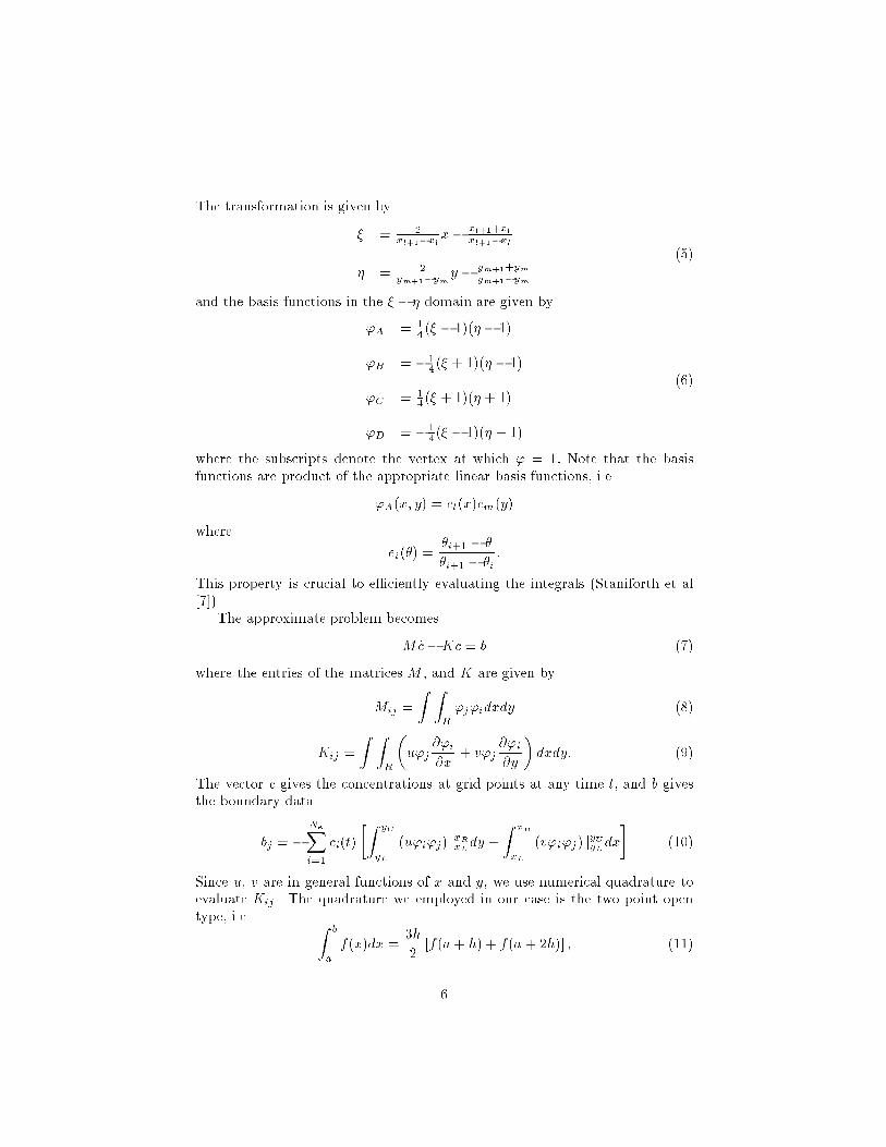
The transformation is given by
� � �xl���xl
x�xl���xlxl���xl
� � �ym���ym
y � ym���ymym���ym
���
and the basis functions in the � � � domain are given by
�A � ���� � ���� � ��
�B � ����� � ���� � ��
�C � ���� � ���� � ��
�D � ����� � ���� � ��
���
where the subscripts denote the vertex at which � � �� Note that the basisfunctions are product of the appropriate linear basis functions� i�e�
�A�x� y� � el�x�em�y�
where
ei��� ��i�� � �
�i�� � �i�
This property is crucial to e�ciently evaluating the integrals �Staniforth et al�� ��
The approximate problem becomes
M �c�Kc � b ���
where the entries of the matrices M � and K are given by
Mij �
Z ZR
�j�idxdy ���
Kij �
Z ZR
�u�j
��i
�x� v�j
��i
�y
�dxdy� ��
The vector c gives the concentrations at grid points at any time t� and b givesthe boundary data
bj � �
NeXi��
ci�t�
�Z yU
yL
�u�i�j� jxRxLdy �
Z xR
xL
�v�i�j� jyUyLdx
�����
Since u� v are in general functions of x and y� we use numerical quadrature toevaluate Kij � The quadrature we employed in our case is the two point opentype� i�e� Z b
a
f�x�dx ��h
��f�a � h� � f�a � �h� � ����
�

where
h �b� a
�
and the error term is given by
�
h�f ������
Thus for the �rst integral in Kij we get
Z ZR
u�j��i
�xdxdy �
NeXk��
Z xl��
xl
Z ym��
ym
u�j��i
�xdxdy� ����
Now use the quadrature for each integral and centered di�erences for the partialderivatives to get
PNek��
��hx
��hy
nu�E��j�E��iP ��iQ�� �
u�H��j�H��iY ��iZ�� �
u�F ��j�F ��iV ��iS�� �
u�G��j�G��iW ��iX��
o
����
�

A B
CD
r r r
E
Q P
r r r
H
Z Y
r r r
F
S V
r r r
G
X W
Figure �� location of quadrature nodes
�
where
hx �xl�� � xl
�� hy �
ym�� � ym
����
and � the spacing for the centered di�erences was arbitrarily chosen as
� ����xl�� � xl�� ����
Similarly� we can approximate the second integral in Kij except that now thepoints will be � ����ym�� � ym� units above and below the four pointsE�F�G�H�
�� Semi�Lagrangian Finite ElementsSemi�Lagrangian schemes belong to the general class of upwinding methods�
For hyperbolic equations� upwinding methods incorporate characteristic infor�mation into the numerical method� In Lagrangian schemes� the evolution of thesystem is monitored by following speci�c �uid particles through space� As aresult� Lagrangian schemes allow larger time steps than Eulerian� The problemwith fully Lagrangian schemes is that an initially regularly spaced set of par�ticles will generally evolve into irregularly spaced particles� As a result� someimportant features in the �ow may not be captured properly� Semi�Lagrangianschemes combine the best of both worlds� the regular resolution of an Eulerianscheme and the high stability of a Lagrangian method� The idea is to choosea di�erent set of particles such that at the end of the time step� they arrive atpoints on a regular Cartesian grid� The departure points of the particles aredetermined by an iterative process using the interpolated velocity vector fromthe previous time�
A semi�Lagrangian formulation of ���
c� � c�
��t�
�
�
h�cux � cvy�� � �cux � cvy��
i� � ����
where c� is the solution at the grid points at time t� �t� c� is the solution attime �t��t� at those points arriving at the grid points at time t��t� Since onerequires two previous time levels� the program uses Matsuno s �see e�g� Haltinerand Williams ��� � method to get the �rst time step�
In the appendix� we bring plots of the solution for the cone test �see e�g�Zlatev �� � using Eulerian �nite elements with explicit� Crank�Nicholson andfully implicit time discretizations as well as the semi�Lagrangian method�
�� Stability AnalysisThere are four rectangles having a vertex in common� as indicated in the
next �gure� The approximate solution at the vertices of the rectangles may beobtained by solving the following �rst order ordinary di�erential equation �seeNeta and Williams �� for the one dimensional advection case��

A R
HF
D E
G
B
P
Figure �� rectangular elements having a common vertex
�c�P � ��� � �c�G� � �c�B� � �c�D� � �c�E�
� ��� � �c�F � � �c�H� � �c�A� � �c�R�
� ���u ��x
fc�H�� c�F � � c�R�� c�A� � �c�E� � c�D� g
� ���v ��y
fc�H� � c�R� � c�F �� c�A� � �c�G�� c�B� g � �
����
Substitute a Fourier mode
c�x� y� t� � A�t�ei�x��y ����
in ���� to get
�A�t�n
� � ���� cos �x� � cos ��y� � �
�� cos �x cos��yo
� ���
u�x
A�t�n
� � cos ��yo
�i sin�x
� ���
v�vA�t�
n � � cos�x
o�i sin ��y � �
���
��

or�A�t� � �i
n u
�x
sin�x
� � cos �x�
v
�y
sin ��y
� � cos ��y
oA�t� � �� ����
For the special case of �ow along the x or y axis one of the terms in braces willdrop� For �ow along the diagonal
u
v�
�y
�x����
we have�A�t� � �i
u
�x
n sin�x
� � cos�x�
sin ��y
� � cos ��y
oA�t� � �� ����
In general� the ordinary di�erential equation becomes
�A�t� � i�A�t� � �� ����
where � is � times the term in braces in ����� For the leap�frog time discretiza�tion
An�� � An�� � �i��tAn � � ���
we have ��� � �i��t �
p�� ����t��� ����
and thus for stability �j j � ��� we must have
j��tj � �� ����
If we letU � max�juj� jvj�
� min��x��y�����
then the method is stable if�t
�
�
�U� ����
This is the CFL condition�
� Fourier Transform
The Fourier transform of a function c�x� y� t� is given by
F fcg � �c�k� l� t� �
Z�
��
Z�
��
c�x� y� t�e�ikx�lydxdy ���
Taking the Fourier transform of the linearization of ���� one gets the initial valueproblem
d�c
dt� i�ku� lv��c � �� ����
��

�c�k� l� �� � �c��k� l�� ����
The solution of which is given by
�c�k� l� t� � �c��k� l�ei�t� ����
where� � ��ku� lv�� ����
To get the solution c�x� y� t� in the physical domain� we have to take the inverseFourier transform and use the convolution theorem� This yields the well knownsolution
c�x� y� t� � c��x� ut� y � vt�� ���
In order to obtain the Fourier transform of the approximate solution� recallthat Z
�
��
u�x� �x� y� t�e�ikxdx � eik�x�u�k� y� t�� ����
Applying Fourier transform to ����� one gets
�c
dt�
�iu
�
�x
sin k�x
� � cos k�x� iv
�
�y
sin l�y
� � cos l�y
��c � �� ����
Compare ���� and ����� to �nd that k� l are replaced by �x� �y respectively�where
�x ��
�x
sin k�x
� � cos k�x� �y �
�
�y
sin l�y
� � cos l�y�
Note that as �x � �� �x � k and as �y � �� �y � l� thus at the limit ����becomes ����� In fact
�x � k ��
���k��x� �
�
����k �x� � O
�k��
�y � l ��
���l��x� �
�
����l �x� � O
�l��
The solution of ���� with the same initial value is given by
�c�k� l� t� � �c��k� l�ei��t� ����
where�� � ���xu� �yv�� ����
The inverse transform is given by
c�x� y� t� ��
��
Z�
��
Z�
��
�c��k� l�e�iu�x�v�yteikx�lydkdl ���
��

or by using convolution
c�x� y� t� � c� � F��ne�iu�x�v�y t
o� ���
� Program Notes
The program can run semi�Lagrangian as well as Eulerian �nite elements�In the Eulerian case the time di�erencing is one of the following�
� Explicit
� Crank Nicholson
� fully implicit
where the resulting linear system of equations is solved by the conjugate gradientmethod with symmetric SOR preconditioning �see e�g� Ortega ��� ��
The four lines of input contain�
�� I� J
�� xL�xR� yL� yU
�� �t� T ��nal time of integration�� IPLOT �number of time steps betweensolution plots��
� � �a parameter dictating the time integrator�� This is needed only forEulerian �nite elements�
Here we include the input �le and the programs used to test the Eulerianand semi�Lagrangian �nite element methods� First we give the input �le� The�rst line contains the number of grid points in the x and y directions� Thesecond line describe the rectangular domain on which the problem is solved�The interval for x is given followed by the interval for y� The third line givesthe time step �t� the �nal time of integration� and the number of time stepsbetween plots� For Eulerian �nite elements� we have a fourth line with the valueof ��
Here is the input �le for the explicit time discretization�
�� ��
��� ��� ��� ���
������ ��� ��
��
��

Here is the program for the Eulerian �nite elements�
�����������������������������������������������������������������������
�This program solves the �D Advection Equation
� dc�dt d�dxcu� d�dycv� � �
�on a square domain using Periodic B�C s
�in both x and y using Bilinear Rectangular Finite Elements
�and THETA Time�Integration Algorithms�
� THETA�� �� FORWARD EULER Explicit�
� THETA���� �� CRANK�NICOLSON Semi�Implicit�
� THETA���� �� GALERKIN Semi�Implicit�
� THETA�� �� BACKWARD EULER Implicit�
�Written by F�X� Giraldo on ����
� NRC Fellow
� Department of Mathematics
� Naval Postgraduate School
� Monterey� CA �����
�����������������������������������������������������������������������
program fem�advect
implicit real��a�h�o�z�
parameter imax��� �
c
c mxpoi max number of points
c mxele max number of elements
c mxbou max number of boundary points
c nd max number of vertices for each elements
c
parameter mx�imax�imax� mxpoi�mx� mxele�mx� mxbou�mx��� nd�� �
c
c global matrices
c
dimension alhsmxpoi�mxpoi�� arhsmxpoi�mxpoi�� bmxpoi�
dimension coordmxpoi���
integer intmamxele�nd�� ibounmxbou���� nodeimax�imax�
c
c u velocity arrays
c
dimension umxpoi�
c
c v velocity arrays
c
dimension vmxpoi�
c
c phi arrays
�

c
dimension phipmxpoi�� phi�mxpoi�
c
c Read the Input Variables and create the Grid
c
c
c input file contains � lines
c on first� number of grid points in x nx� and y ny� direction
c on second�range of x values xmin� xmax��
c range of y values ymin�ymax�
c on third� delta t�
c final time of integration time�final��
c number of times steps between plots iplot�
c on fourth� theta see above�
c
call initphi��u�v�node�coord�intma�iboun�npoin�nelem�
� nboun�xmin�xmax�ymin�ymax�ym�nx�ny�nd�dx�dy�dt�
� ntime�theta�mxpoi�mxele�mxbou�imax�iplot�
pi�����atan����
open��file� matlab�out �
c
c isets � number of time steps at which solution is plotted
c
isets�ntime�iplot �
write����isets
c
c always plot initial condition
c
call outputphi��u�v�npoin�time�nx�ny�mxpoi�
c
c begin the time marching
c
time����
c
c CREATE THE STIFFNESS MATRIX ONCE
c
call lhsalhs�arhs�coord�intma�iboun�node�u�v�npoin�nelem�
� nboun�nx�ny�nd�dx�dy�dt�theta�mxpoi�mxele�mxbou�imax�
do i���npoin
do j���npoin
c write����i�j�alhsi�j�
end do
end do
c
��

c TIME MARCH
c
do itime���ntime
time�time dt
write�� � timestep time � ��i���x�e����� �itime�time�����pi�
c
c Solve for the GeoPotential
c
call rhsb�arhs�phi��coord�intma�iboun�node�
� npoin�nelem�nboun�nx�ny�nd�dx�dy�
� mxpoi�mxele�mxbou�imax�
if theta�eq����� then
call solve�explicitalhs�phip�b�npoin�mxpoi�
else if theta�ne����� then
call pcgmalhs�phip�b�npoin�mxpoi�
endif
c
c Enforce B�C�s Explicitly
c
do i���nx
j��nodei���
jny�nodei�ny�
phipj���phipjny�
end do
do j���ny
i��node��j�
inx�nodenx�j�
phipi���phipinx�
end do
c
c Update
c
do ip���npoin
phi�ip��phipip�
end do
c
c check printing status
c
if moditime�iplot��eq���
� call outputphi��u�v�npoin�time�nx�ny�mxpoi�
end do
��

���� continue
call outputphi��u�v�npoin�time�nx�ny�mxpoi�
close��
stop
end
�����������������������������������������������������������������������
�This subroutine writes the output� It is currently set only to
�print the concentration or color� function at each node point�
�Written by F�X� Giraldo on ����
�����������������������������������������������������������������������
subroutine outputphi�u�v�npoin�time�nx�ny�mxpoi�
implicit real��a�h�o�z�
dimension phimxpoi�� umxpoi�� vmxpoi�
pi�����atan����
write�� �i���x��e����� ��nx�ny�time�����pi�
write�� e����� �phiip�� ip���npoin�
return
end
�����������������������������������������������������������������������
�This subroutine reads in the input file�
�The info read is the number of grid points in x and y�� the domain�
�the time step� the final time� and the number of time steps for plotting�
�Written by F�X� Giraldo on ����
�����������������������������������������������������������������������
subroutine initphi��u��v��node�coord�intma�iboun�npoin�nelem�
� nboun�xmin�xmax�ymin�ymax�ym�nx�ny�nd�dx�dy�dt�
� ntime�theta�mxpoi�mxele�mxbou�imax�iplot�
implicit real��a�h�o�z�
dimension coordmxpoi���
dimension phi�mxpoi�� u�mxpoi�� v�mxpoi�
integer intmamxele�nd�� ibounmxbou���� nodeimax�imax�
c
c Read Input File
c
read����nx�ny
read����xmin�xmax�ymin�ymax
read����dt�time�final�iplot
read����theta
c
c check bounds
c
if nx�ny�gt�mxpoi� then
��

write�� � Error� � Need to Enlarge MXPOI�� �
stop
else if nx����ny����gt�mxele� then
write�� � Error� � Need to Enlarge MXELE�� �
stop
else if ��nx�����ny����gt�mxbou� then
write�� � Error� � Need to Enlarge MXBOU�� �
stop
endif
c
c set some constants
c
pi�����atan����
ntime�ninttime�final�dt�
dt�dt�����pi
time�final�time�final�����pi
xm�����xmaxxmin�
ym�����ymaxymin�
dx�xmax�xmin��nx���
dy�ymax�ymin��ny���
xl�xmax�xmin
yl�ymax�ymin
w����
cx������xl
cy������yl
h������
rc�������xl
velmax���e�
c
c set the Initial Conditions
c
ip��
do j���ny
y�ymin realj����dy
do i���nx
x�xmin reali����dx
ip�ip�
r�sqrt x�cx���� y�cy���� �
phi�ip�����
if r�lt�rc� then
phi�ip��h�����r�rc�
endif
u�ip��y�ym�
v�ip���x�xm�
��

vel��u�ip���� v�ip����
velmax�maxvelmax�vel��
end do
end do
cfl�dt�sqrtvelmax�dx��� dy�����
print�� �� CFL � �cfl
c
c GENERATE COORD
c
npoin�nx�ny
ip��
do j���ny
do i���nx
ip�ip�
nodei�j��ip
coordip����xi dx�reali���
coordip����yi dy�realj���
end do
end do
c
c GENERATE INTMA
c
nelem�nx����ny���
ie��
do j���ny��
do i���nx��
ie�ie�
intmaie����nodei�j�
intmaie����nodei��j�
intmaie����nodei��j��
intmaie����nodei�j��
end do
end do
c
c GENERATE IBOUN
c
nboun���nx��� ��ny���
ib��
c bottom y�ymin�
ie��
do i���nx��
ib�ib�
ibounib����nodei���
�

ibounib����nodei����
ibounib����ie
ibounib�����
ie�ie�
end do
c top y�ymax�
ie�nelem
do i�nx�����
ib�ib�
ibounib����nodei�ny�
ibounib����nodei���ny�
ibounib����ie
ibounib�����
ie�ie��
end do
c right x�xmax�
ie�nx���
do j���ny��
ib�ib�
ibounib����nodenx�j�
ibounib����nodenx�j��
ibounib����ie
ibounib�����
ie�ie nx���
end do
c left x�xmin�
ie�nelem � nx��� �
do j�ny�����
ib�ib�
ibounib����node��j�
ibounib����node��j���
ibounib����ie
ibounib�����
ie�ie � nx���
end do
return
end
�����������������������������������������������������������������������
�This subroutine constructs the LHS matrix for Bilinear Rectangular
�Elements for the Advection Equation with Periodic
��

�East�West and North�South Boundary Conditions�
�Written by F�X� Giraldo on ����
�����������������������������������������������������������������������
subroutine lhsalhs�arhs�coord�intma�iboun�node�u�v�npoin�nelem�
� nboun�nx�ny�nd�dx�dy�dt�theta�mxpoi�mxele�mxbou�imax�
implicit real��a�h�o�z�
parameter mx������
c
c global arrays
c
dimension alhsmxpoi�mxpoi�� arhsmxpoi�mxpoi�
dimension coordmxpoi���� umxpoi�� vmxpoi�
integer intmamxele�nd�� nodeimax�imax�� ibounmxbou���
c
c local coordinate system for a CCW ordered rectangle
c
dimension xi��� eta��� a�tempmx�
data xi ���� �� ���� �
data eta ������� �� � �
c
c initialize the global matrix
c
do j���npoin
do i���npoin
alhsi�j�����
arhsi�j�����
end do
end do
c
c loop thru the elements
c
do ie���nelem
c
c assemble element matrix cm �� consistent mass matrix
c ckc �� conduction�like matrix
do i���nd
ii�intmaie�i�
cm�lump����
do j���nd
jj�intmaie�j�
cm������������xii��xij��������������etai��etaj��
ckx����
cky����
do k���nd
��

uk�uintmaie�k��
vk�vintmaie�k��
ckx�ckx uk�
� ����xii� ��������xii��xij��xik���
� �����������etai��etaj� etai��etak� etaj��etak���
cky�cky vk�
� ����etai� ��������etai��etaj��etak���
� �����������xii��xij� xii��xik� xij��xik���
end do
cmm�dx�dy������cm
ck�dy�������ckx dx�������cky
alhsii�jj��alhsii�jj� ����dt�cmm � theta�ck
arhsii�jj��arhsii�jj� ����dt�cmm ����theta��ck
end do
end do
end do
c
c Account for Periodicity
c
do i���nx
j��nodei���
jny�nodei�ny�
do jj���npoin
a�tempjj��alhsj��jj� alhsjny�jj�
end do
do jj���npoin
alhsj��jj��a�tempjj�
alhsjny�jj��a�tempjj�
end do
alhsj��j���a�tempj�� a�tempjny�
alhsjny�jny��a�tempj�� a�tempjny�
end do
do j���ny
i��node��j�
inx�nodenx�j�
do jj���npoin
a�tempjj��alhsi��jj� alhsinx�jj�
end do
do jj���npoin
alhsi��jj��a�tempjj�
alhsinx�jj��a�tempjj�
end do
alhsi��i���a�tempi�� a�tempinx�
��

alhsinx�inx��a�tempi�� a�tempinx�
end do
c
c If theta��� then Lump�
c
if theta�eq����� then
do i���npoin
asum����
do j���npoin
asum�asum alhsi�j�
alhsi�j�����
end do
alhsi�i��asum
end do
endif
return
end
�����������������������������������������������������������������������
�The next � Subroutines solve a linear system �A��x���b�� for n unknowns using
�the CONJUGATE GRADIENT METHOD with an SSOR preconditioner�
�The variable w determines the preconditioner� for w�� it is
�Symmetric Jacobi and for w�� it is Symmetric SOR SSOR��
�Written by F�X� Giraldo on �������
�Modified for any type of spd Matrix A on ����
�����������������������������������������������������������������������
subroutine pcgma�x�b�n�mx�
implicit real��a�h�o�z�
parameter nmax������ kmax���� w�����
dimension amx�mx�� bmx�� xmx�
dimension rnmax�� rwnmax�� pnmax�� apnmax�
do i���n
sum����
do j���n
sum�sum ai�j��xj�
end do
ri��bi� � sum
end do
call ssorr�rw�a�n�w�nmax�mx�
do i���n
pi��rwi�
��

end do
call iprop�rw�r�n�nmax�
do k���kmax
do i���n
sum����
do j���n
sum�sum ai�j��pj�
end do
api��sum
end do
alfden����
do i���n
alfden�alfden pi��api�
end do
alf��rop�alfden
do i���n
xi��xi��alf�pi�
end do
do i���n
ri��ri� alf�api�
end do
call convtestrop�r�n�flag�nmax�
if flag �eq� ���� goto ���
call ssorr�rw�a�n�w�nmax�mx�
call iprnp�rw�r�n�nmax�
beta�rnp�rop
do i���n
pi��rwi� beta�pi�
end do
rop�rnp
end do
k�k��
print�� No Convergence
��� continue
�

print�� SSOR PCG Loops � �k
return
end
�����������������������������������������������������������������������
subroutine ssorr�rw�a�n�w�nmax�mx�
implicit real��a�h�o�z�
dimension rnmax�� rwnmax�
dimension amx�mx�
� symmetric sor on the residual
� zeroing the wiggle residual
do i���n
rwi�����
end do
� up sweep
do i���n
sum����
do j���n
sum�sum ai�j��rwj�
end do
rwi��rwi� w�ai�i�� ri� � sum �
end do
� down sweep
do i�n�����
sum����
do j���n
sum�sum ai�j��rwj�
end do
rwi��rwi� w�ai�i�� ri� � sum �
end do
return
end
�����������������������������������������������������������������������
subroutine ipf�fw�fr�n�nmax�
implicit real��a�h�o�z�
dimension fwnmax�� frnmax�
f����
do i���n
f�f fwi��fri�
��

end do
return
end
�����������������������������������������������������������������������
subroutine convtestrop�r�n�flag�nmax�
implicit real��a�h�o�z�
dimension rnmax�
emin����e��
flag����
rtest����
if rop �lt� emin� then
do i���n
rtest�rtest ri������
end do
if rtest �lt� emin� flag����
endif
return
end
�����������������������������������������������������������������������
�This subroutine Builds the RHS vector for Bilinear Rectangular Finite
�Elements for the �D SLSI Shallow Water Equations with Periodic
�West�East and North�South Boundaries�
�Written by F�X� Giraldo on ����
�����������������������������������������������������������������������
subroutine rhsb�arhs�phi��coord�intma�iboun�node�
� npoin�nelem�nboun�nx�ny�nd�dx�dy�
� mxpoi�mxele�mxbou�imax�
implicit real��a�h�o�z�
parameter mx������
c
c global arrays
c
dimension bmxpoi�� arhsmxpoi�mxpoi�� phi�mxpoi�
dimension coordmxpoi���
integer intmamxele�nd�� ibounmxbou���� nodeimax�imax�
c
c local coordinates for a CCW ordered Rectangle
c
dimension xi��� eta��
data xi ���� �� �����
data eta ������� �� ��
c
c initialize the right hand side
��

c
do ip���npoin
bip�����
end do
c
c Construct the RHS Vector
c
do i���npoin
do j���npoin
bi��bi� arhsi�j��phi�j�
end do
end do
c
c Account for Periodicity
c
do i���nx
j��nodei���
jny�nodei�ny�
b�temp�bj�� bjny�
bj���b�temp
bjny��b�temp
end do
do j���ny
i��node��j�
inx�nodenx�j�
b�temp�bi�� binx�
bi���b�temp
binx��b�temp
end do
return
end
�����������������������������������������������������������������������
�This subroutine solves a Linear NxN system where the Coefficient
�Matrix is diagonal�
�Written by F�X� Giraldo on �������
�����������������������������������������������������������������������
subroutine solve�explicita�x�b�n�mx�
implicit real��a�h�o�z�
dimension amx�mx�� bmx�� xmx�
do i���n
xi��bi��ai�i�
end do
return
end
��

Here is the program for the semi�Lagrangian �nite elements�
�����������������������������������������������������������������������
�This program solves the �D Advection Equation
� dc�dt d�dxcu� d�dycv� � �
�on a square domain using Periodic B�C� s
�in both x and y and using Semi�Implicit Semi�Lagrangian
�Bilinear Rectangular Finite Elements�
�Written by F�X� Giraldo on ����
� NRC Fellow
� Department of Mathematics
� Naval Postgraduate School
� Monterey� CA �����
�����������������������������������������������������������������������
program slt�advect
implicit real��a�h�o�z�
parameter imax��� �
c
c mxpoi max number of points
c mxele max number of elements
c mxbou max number of boundary points
c nd max number of vertices for each elements
c
parameter mx�imax�imax� mxpoi�mx� mxele�mx� mxbou�mx��� nd�� �
c
c global matrices
c
dimension amxpoi�mxpoi�� bmxpoi�
dimension fmxpoi�
dimension coordmxpoi���
dimension cmatmxpoi�
integer intmamxele�nd�� ibounmxbou���
c
c u velocity arrays
c
dimension ummxpoi�� u�mxpoi�� upmxpoi�
dimension u��xmxpoi�
c
c v velocity arrays
c
dimension vmmxpoi�� v�mxpoi�� vpmxpoi�
dimension v��ymxpoi�
c
c phi arrays
��

c
dimension phimmxpoi�� phi�mxpoi�� phipmxpoi�
c
c departure point arrays
c
dimension alfmmxpoi���� alf�mxpoi���
c
c spline derivative arrays
c
dimension dphimmxpoi�
dimension du�mxpoi�� du��xmxpoi�
dimension dv�mxpoi�� dv��ymxpoi�
c
c Auxiliary Matrices
c
integer nodeimax�imax�
c
c Read the Input Variables and create the Grid
c
c input file contains � lines
c on first� number of grid points in x nx� and y ny� direction
c on second�range of x values xmin� xmax��
c range of y values ymin�ymax�
c on third� delta t�
c final time of integration time�final��
c number of times steps between plots iplot�
c
call initphi��u��v��node�coord�alf��intma�iboun�npoin�
� nelem�nboun�xmin�xmax�ymin�ymax�nx�ny�dx�dy�dt�
� ntime�ym�nd�mxpoi�mxele�mxbou�imax�iplot�
c
c Construct the Lumped Mass Matrix used for the derivative computation
c
call get�geomnelem�npoin�intma�coord�cmat�node�
� nx�ny�nd�dx�dy�mxpoi�mxele�imax�
time����
pi�����atan����
open��file� matlab�out �
c
c isets � number of time steps at which solution is plotted
c
isets�ntime�iplot �
write����isets
c
�

c always plot initial condition
c
call outputphi��u��v��npoin�time�nx�ny�mxpoi�
c
c begin the time marching
c
c Do the �st Time�step Integration to get ��time levels
c
do itime����
time�time dt
dtime�time�����pi�
write�� � timestep time � ��i���x�e����� �itime�dtime
call matsunophim�phi��phip�um�u��up�
� vm�v��vp�coord�intma�npoin�nelem�dt�dx�dy�
� node�nx�ny�ym�nd�mxpoi�mxele�imax�
call updatephim�phi��phip�um�u��up�vm�v��vp�alfm�alf��
� npoin�mxpoi�
end do
c
c TIME MARCH
c
do itime���ntime
time�time dt
dtime�time�����pi�
write�� � timestep time � ��i���x�e����� �itime�dtime
�
� �st� DETERMINE DEPARTURE POINT
�
call splie�du��u��coord�nx�ny�node�mxpoi�imax�
call splie�dv��v��coord�nx�ny�node�mxpoi�imax�
call departalf��alfm�coord�u��du��v��dv��
� npoin�dt�xmin�xmax�ymin�ymax�
� nd�mxpoi�node�nx�ny�imax�
�
� �nd� COMPUTE DERIVATIVES
�
call deriv�xu��x�u��intma�cmat�node�npoin�nelem�
� nx�ny�nd�dy�mxpoi�mxele�imax�
call deriv�yv��y�v��intma�cmat�node�npoin�nelem�
� nx�ny�nd�dx�mxpoi�mxele�imax�
�
� �rd� INTERPOLATE PHIM� UM�X�U��X� VM�Y�V��Y
� at the departure point � X � ��ALPHA
��

�
call splie�dphim�phim�coord�nx�ny�node�mxpoi�imax�
call splie�du��x�u��x�coord�nx�ny�node�mxpoi�imax�
call splie�dv��y�v��y�coord�nx�ny�node�mxpoi�imax�
c
c INTERPOLATE THE RIGHT HAND SIDE FUNCTION
c
call interpf�phim�u��x�v��y�dphim�du��x�dv��y�coord�
� alf��node�npoin�dt�xmin�xmax�ymin�ymax�ym�
� nx�ny�nd�mxpoi�imax�
do ip���npoin
phipip��fip�
upip��u�ip�
vpip��v�ip�
end do
c
c Update the values
c
call updatephim�phi��phip�um�u��up�vm�v��vp�alfm�alf��
� npoin�mxpoi�
c
c check time for printing output
c
if moditime�iplot��eq���
� call outputphi��u��v��npoin�time�nx�ny�mxpoi�
end do
���� continue
call outputphi��u��v��npoin�time�nx�ny�mxpoi�
close��
stop
end
�����������������������������������������������������������������������
�This subroutine finds the departure point
� ALPHA��DT�UX�ALPHA��Y�ALPHA��T� ALPHA��DT�VX�ALPHA��Y�ALPHA��T�
�Written by F�X� Giraldo on ����
�����������������������������������������������������������������������
subroutine departalf��alfm�coord�u��du��v��dv��
� npoin�dt�xmin�xmax�ymin�ymax�
� nd�mxpoi�node�nx�ny�imax�
implicit real��a�h�o�z�
dimension alf�mxpoi���� alfmmxpoi���
��

dimension u�mxpoi�� du�mxpoi�
dimension v�mxpoi�� dv�mxpoi�
dimension coordmxpoi���
integer nodeimax�imax�
do ip���npoin
alpha��alfmip���
alpha��alfmip���
do k����
xd�coordip��� � alpha�
yd�coordip��� � alpha�
if xd�lt�xmin� xd�xmax � xmin � xd�
if xd�gt�xmax� xd�xmin xd � xmax�
if yd�lt�ymin� yd�ymax � ymin � yd�
if yd�gt�ymax� yd�ymin yd � ymax�
if xd�lt�xmin�or�xd�gt�xmax� �or�
� yd�lt�ymin�or�yd�gt�ymax� � then
print�� Error in DEPART
print�� XD out of Range � �xd�yd
print�� ip alpha � �ip�alpha��alpha�
stop
endif
call splin�u�coord�u��du��xd�yd�nx�ny�node�mxpoi�imax�
call splin�v�coord�v��dv��xd�yd�nx�ny�node�mxpoi�imax�
alpha��dt�u
alpha��dt�v
end do
alf�ip����alpha�
alf�ip����alpha�
end do
return
end
�����������������������������������������������������������������������
�This subroutine computes the �th Order Accurate derivative WRT X of the
�variable UNKNO and stores it in DERIP using Bilinear Rectangular
�Finite Elements
�Written by F�X� Giraldo on ����
�����������������������������������������������������������������������
subroutine deriv�xderip�unkno�intma�cmat�node�npoin�nelem�
� nx�ny�nd�dy�mxpoi�mxele�imax�
��

implicit real��a�h�o�z�
c
c global arrays
c
dimension deripmxpoi�� unknomxpoi�
dimension cmatmxpoi�
integer intmamxele�nd�� nodeimax�imax�
c
c local coordinate system for a CCW ordered rectangle
c
dimension xi��� eta��
data xi � ��� �� ���� �
data eta � ������ �� � �
c
c initialize arrays
c
do ip���npoin
deripip�����
end do
c
c Loop thru the Elements and find the �St DERIVATIVES
c
do ie���nelem
do i���nd
phi�x����
ip�intmaie�i�
do k���nd
phik�unknointmaie�k��
phi�x�phi�x xik��phik� ��� ��������etak��etai� �
end do
deripip��deripip� dy������phi�x
end do
end do
c
c Account for Periodicity
c
do j���ny
i��node��j�
inx�nodenx�j�
derip�temp�deripi�� deripinx�
deripi���derip�temp
deripinx��derip�temp
end do
c
��

c Now multiply by the Inverse of the Lumped mass matrix
c
do ip���npoin
deripip��deripip��cmatip�
end do
return
end
�����������������������������������������������������������������������
�This subroutine computes the �th Order Accurate derivative WRT Y of the
�variable UNKNO and stores it in DERIP using Bilinear Rectangular
�Finite Elements
�Written by F�X� Giraldo on ����
�����������������������������������������������������������������������
subroutine deriv�yderip�unkno�intma�cmat�node�npoin�nelem�
� nx�ny�nd�dx�mxpoi�mxele�imax�
implicit real��a�h�o�z�
c
c global arrays
c
dimension deripmxpoi�� unknomxpoi�
dimension cmatmxpoi�
integer intmamxele�nd�� nodeimax�imax�
c
c local coordinate system for a CCW ordered rectangle
c
dimension xi��� eta��
data xi � ��� �� ���� �
data eta � ������ �� � �
c
c initialize arrays
c
do ip���npoin
deripip�����
end do
c
c Loop thru the Elements and find the �St DERIVATIVES
c
do ie���nelem
do i���nd
phi�y����
ip�intmaie�i�
do k���nd
phik�unknointmaie�k��
�

phi�y�phi�y etak��phik� ��� ��������xik��xii� �
end do
deripip��deripip� dx������phi�y
end do
end do
c
c Account for Periodicity
c
do j���ny
i��node��j�
inx�nodenx�j�
derip�temp�deripi�� deripinx�
deripi���derip�temp
deripinx��derip�temp
end do
c
c Now multiply by the Inverse of the Lumped mass matrix
c
do ip���npoin
deripip��deripip��cmatip�
end do
return
end
�����������������������������������������������������������������������
�This subroutine computes the Inverse Lumped Mass Matrix
�for Bilinear Rectangular Finite Elements used for obtaining the
��th Order Accurate �st and �nd derivatives in both X and Y�
�Written by F�X� Giraldo on ����
�����������������������������������������������������������������������
subroutine get�geomnelem�npoin�intma�coord�cmat�node�
� nx�ny�nd�dx�dy�mxpoi�mxele�imax�
implicit real��a�h�o�z�
c
c global arrays
c
dimension coordmxpoi���� cmatmxpoi�
integer intmamxele�nd�� nodeimax�imax�
c
c Compute the inverse lumped mass matrix
c
do ip���npoin
cmatip�����
end do
��

do ie���nelem
do in���nd
ip�intmaie�in�
cmatip��cmatip� dx�dy����
end do
end do
c
c Account for Periodicity in X
c
do j���ny
i��node��j�
inx�nodenx�j�
cmat�temp�cmati�� cmatinx�
cmati���cmat�temp
cmatinx��cmat�temp
end do
c
c Invert the lumped mass matrix
c
do ip���npoin
cmatip������cmatip�
end do
return
end
�����������������������������������������������������������������������
�This subroutine reads in the input file�
�The info read is the number of grid points in x and y�� the domain�
�the time step� the final time� and the number of time steps for plotting�
�Written by F�X� Giraldo on ����
�����������������������������������������������������������������������
subroutine initphi��u��v��node�coord�alf��intma�iboun�npoin�
� nelem�nboun�xmin�xmax�ymin�ymax�nx�ny�dx�dy�dt�
� ntime�ym�nd�mxpoi�mxele�mxbou�imax�iplot�
implicit real��a�h�o�z�
dimension coordmxpoi���� alf�mxpoi���
dimension phi�mxpoi�� u�mxpoi�� v�mxpoi�
integer intmamxele�nd�� ibounmxbou���� nodeimax�imax�
c
c Read Input File
c
read����nx�ny
read����xmin�xmax�ymin�ymax
��
read����dt�time�final�iplot
c
c check bounds
c
if nx�ny�gt�mxpoi� then
write�� � Error� � Need to Enlarge MXPOI�� �
stop
else if nx����ny����gt�mxele� then
write�� � Error� � Need to Enlarge MXELE�� �
stop
else if ��nx�����ny����gt�mxbou� then
write�� � Error� � Need to Enlarge MXBOU�� �
stop
endif
c
c set some constants
c
pi�����atan����
ntime�ninttime�final�dt�
dt�dt�����pi
time�final�time�final�����pi
xm�����xmaxxmin�
ym�����ymaxymin�
dx�xmax�xmin��nx���
dy�ymax�ymin��ny���
xl�xmax�xmin
yl�ymax�ymin
w����
cx������xl
cy������yl
h������
rc�������xl
velmax���e�
c
c set the Initial Conditions
c
ip��
do j���ny
y�ymin realj����dy
do i���nx
x�xmin reali����dx
ip�ip�
r�sqrt x�cx���� y�cy���� �
phi�ip�����
��

if r�lt�rc� then
phi�ip��h�����r�rc�
endif
u�ip��y�ym�
v�ip���x�xm�
vel��u�ip���� v�ip����
velmax�maxvelmax�vel��
end do
end do
cfl�dt�sqrtvelmax�dx��� dy�����
print�� �� CFL � �cfl
c
c GENERATE COORD
c
npoin�nx�ny
ip��
do j���ny
do i���nx
ip�ip�
nodei�j��ip
coordip����xi dx�reali���
coordip����yi dy�realj���
alf�ip��������dx
alf�ip��������dy
end do
end do
c
c GENERATE INTMA
c
nelem�nx����ny���
ie��
do j���ny��
do i���nx��
ie�ie�
intmaie����nodei�j�
intmaie����nodei��j�
intmaie����nodei��j��
intmaie����nodei�j��
end do
end do
c
c GENERATE IBOUN
c
nboun���nx���
��

ib��
c bottom y�ymin�
ie��
do i���nx��
ib�ib�
ibounib����nodei���
ibounib����nodei����
ibounib����ie
ibounib�����
ie�ie�
end do
c top y�ymax�
ielem�nelem
do i�nx�����
ib�ib�
ibounib����nodei�ny�
ibounib����nodei���ny�
ibounib����ielem
ibounib�����
ielem�ielem��
end do
return
end
�����������������������������������������������������������������������
�This subroutine interpolates the right hand side function for the
��D Advection Equation using a ��time level Semi�Lagrangian
�Semi�Implicit Method
�Written by F�X� Giraldo on ����
�����������������������������������������������������������������������
subroutine interpf�phim�u��x�v��y�dphim�du��x�dv��y�coord�
� alf��node�npoin�dt�xmin�xmax�ymin�ymax�ym�
� nx�ny�nd�mxpoi�imax�
implicit real��a�h�o�z�
dimension fmxpoi�
dimension phimmxpoi�� u��xmxpoi�� v��ymxpoi�
dimension dphimmxpoi��du��xmxpoi��dv��ymxpoi�
dimension coordmxpoi���� alf�mxpoi���
integer nodeimax�imax�
do ip���npoin
c
�

c �st� Interpolate ��� values � F x � ��alpha� t � dt �
c
xd�coordip��� � ����alf�ip���
yd�coordip��� � ����alf�ip���
if xd�lt�xmin� xd�xmax � xmin � xd�
if xd�gt�xmax� xd�xmin xd � xmax�
if yd�lt�ymin� yd�ymax � ymin � yd�
if yd�gt�ymax� yd�ymin yd � ymax�
if xd�lt�xmin�or�xd�gt�xmax� �or�
� yd�lt�ymin�or�yd�gt�ymax� � then
print�� Error in INTERP
print�� XD out of Range � �xd�yd
stop
endif
c Do Interpolation
call splin�phi�coord�phim�dphim�xd�yd�nx�ny�node�mxpoi�imax�
call splin�u�x�coord�u��x�du��x�xd�yd�nx�ny�node�mxpoi�imax�
call splin�v�y�coord�v��y�dv��y�xd�yd�nx�ny�node�mxpoi�imax�
fip������dt�u�x v�y������dt�u��xip� v��yip����phi
end do
return
end
�����������������������������������������������������������������������
�This subroutine solves the �D Advection Equation
�using the Backward Euler with a predictor�corrector strategy
�Written by F�X� Giraldo on ����
�����������������������������������������������������������������������
subroutine matsunophim�phi��phip�um�u��up�
� vm�v��vp�coord�intma�npoin�nelem�dt�dx�dy�
� node�nx�ny�ym�nd�mxpoi�mxele�imax�
implicit real��a�h�o�z�
dimension phimmxpoi�� phi�mxpoi�� phipmxpoi�
dimension ummxpoi�� u�mxpoi�� upmxpoi�
dimension vmmxpoi�� v�mxpoi�� vpmxpoi�
dimension coordmxpoi���
integer intmamxele�nd�� nodeimax�imax�
c
c Loop through the points and integrate using Forward Time
c and Centered Space���
c
�

� Predictor Stage forward Euler�
do j���ny
j��j��
j��j�
if j��lt��� j��ny��
if j��gt�ny� j���
do i���nx
i��i��
i��i�
if i��lt��� i��nx��
if i��gt�nx� i���
c
c Set up the nodes in X and Y
c
ip�nodei�j�
ip��nodei��j�
ip��nodei��j�
jp��nodei�j��
jp��nodei�j��
c
c integrate PHI
c
phimip��phi�ip�
� �����dt�dx�u�ip�� phi�ip���phi�ip�� �
� �����dt�dy�v�ip�� phi�jp���phi�jp�� �
c
c integrate U
c
umip��u�ip�
c
c integrate V
c
vmip��v�ip�
end do
end do
� Corrector Stage backward Euler�
do j���ny
j��j��
j��j�
�

if j��lt��� j��ny��
if j��gt�ny� j���
do i���nx
i��i��
i��i�
if i��lt��� i��nx��
if i��gt�nx� i���
c
c Set up the nodes in X and Y
c
ip�nodei�j�
ip��nodei��j�
ip��nodei��j�
jp��nodei�j��
jp��nodei�j��
c
c integrate PHI
c
phipip��phi�ip�
� �����dt�dx�umip�� phimip���phimip�� �
� �����dt�dy�vmip�� phimjp���phimjp�� �
c
c integrate U
c
upip��u�ip�
c
c integrate V
c
vpip��v�ip�
end do
end do
c
c Apply the Periodic Boundary Conditions
c
do j���ny
i��node��j�
i��nodenx�j�
phipi���phipi��
upi���upi��
vpi���vpi��
end do
do i���nx
�

i��nodei���
i��nodei�ny�
phipi���phipi��
upi���upi��
vpi���vpi��
end do
���� continue
return
end
�����������������������������������������������������������������������
�This subroutine writes the output� It is currently set only to
�print the concentration or color� function at each node point�
�Written by F�X� Giraldo on ����
�����������������������������������������������������������������������
subroutine outputphi�u�v�npoin�time�nx�ny�mxpoi�
implicit real��a�h�o�z�
dimension phimxpoi�� umxpoi�� vmxpoi�
pi�����atan����
write�� �i���x��e����� ��nx�ny�time�����pi�
write�� e����� �phiip�� ip���npoin�
return
end
�����������������������������������������������������������������������
�These next � subroutines construct the Hermitian Interpolation functions
�required by the semi�Lagrangian method�
�Obtained from Numerical Recipes�
�Written by F�X� Giraldo on ����
�����������������������������������������������������������������������
subroutine splie�df�f�coord�nx�ny�node�mxpoi�imax�
implicit real��a�h�o�z�
parameter nmax������
c
c global arrays
c
dimension coordmxpoi���� fmxpoi�� dfmxpoi�
integer nodeimax�imax�
c
c local arrays
c
dimension xnmax�� ynmax�� y�nmax�
�

do j���ny
do i���nx
yi��fnodei�j��
xi��coordnodei�j����
end do
call spliney��y�x�nx�idum�nmax�
do i���nx
dfnodei�j���y�i�
end do
end do
return
end
�����������������������������������������������������������������������
subroutine splin�fd�coord�f�df�xd�yd�nx�ny�node�mxpoi�imax�
implicit real��a�h�o�z�
parameter nmax������
c
c global arrays
c
dimension coordmxpoi���� fmxpoi�� dfmxpoi�
integer nodeimax�imax�
c
c local arrays
c
dimension xnmax�� ynmax�� y�nmax�� y��nmax�
do j���ny
do i���nx
yi��fnodei�j��
y�i��dfnodei�j��
xi��coordnodei�j����
end do
call splintfd�x�y�y��xd�nx�nmax�
y��j��fd
end do
do j���ny
xj��coordnode��j����
yj��y��j�
end do
call spliney��y�x�ny�idum�nmax�
call splintfd�x�y�y��yd�nx�nmax�
return

end
�����������������������������������������������������������������������
subroutine spliney��y�x�n�idum�mx�
implicit real��a�h�o�z�
parameter nmax������
dimension ymx�� y�mx�� xmx�� unmax�
if mx�gt�nmax� then
write�� � Must expand NMAX in Subroutine Spline�� �
stop
endif
y�������
u������
do i���n��
sig�xi��xi�����xi���xi����
p�sig�y�i��� ���
y�i��sig � �����p
ui������yi���yi���xi���xi�� � yi��yi����
� �xi��xi������xi���xi�����sig�ui�����p
end do
y�n�����
do i�n�������
y�i��y�i��y�i�� ui�
end do
return
end
�����������������������������������������������������������������������
subroutine splintyd�x�y�y��xd�n�mx�
implicit real��a�h�o�z�
dimension xmx�� ymx�� y�mx�
i���
i��n
�� if i��i��gt��� then
im�i�i����
if xd�gt�xim�� then
i��im
else
i��im
endif
goto ��
endif
�

x��xi��
x��xi��
dx�x��x�
a�x��xd��dx
b�xd�x���dx
yd�a�yi�� b�yi��
� a����a��y�i�� b����b��y�i����dx��������
return
end
�����������������������������������������������������������������������
�This subroutine updates the arrays PHIM�UM�VM�ALFM� PHI��U��V��ALF�
�Written by F�X� Giraldo on ����
�����������������������������������������������������������������������
subroutine updatephim�phi��phip�um�u��up�vm�v��vp�alfm�alf��
� npoin�mxpoi�
implicit real��a�h�o�z�
dimension phimmxpoi�� phi�mxpoi�� phipmxpoi�
dimension ummxpoi�� u�mxpoi�� upmxpoi�
dimension vmmxpoi�� v�mxpoi�� vpmxpoi�
dimension alfmmxpoi���� alf�mxpoi���
c
c Loop through all the nodes and update
c
do ip���npoin
c
c Update Fx���alpha�t�dt��Fx�alpha�t�
c
phimip��phi�ip�
umip��u�ip�
vmip��v�ip�
alfmip����alf�ip���
alfmip����alf�ip���
c
c Update Fx�alpha�t��Fx�tdt�
c
phi�ip��phipip�
u�ip��upip�
v�ip��vpip�
end do
return
end
�
A Matlab Program to plot the output showing the cone at various time isgiven
clg
i���
j���
fid�fopen matlab�out � r ��
ab�fscanffid� �d ����
isets�ab��
while i isets�
ab�fscanffid� �d�d�f ����
nx�ab��
ny�ab��
hour�ab��
count�nx�ny�
jj���
while j ny�
�aa�count��fscanffid� �e�e�e�e�e �nx��
abjj�jjcount����aa�
j�j��
jj�jjcount�
end�
u�reshapeab�nx�ny��
v�u �
c�contourv�����
clabelc��
title� concentration after �num�strhour�� revolutions ��
print c �dps �append
i�i��
j���
end�
�

Conclusion
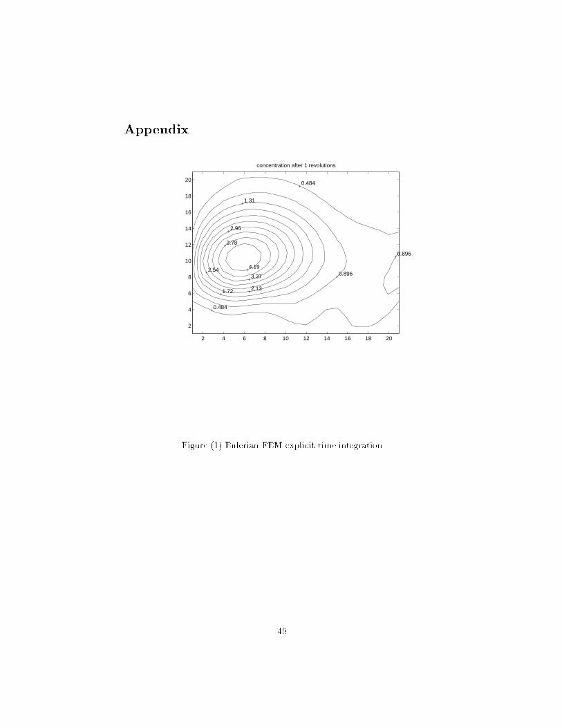
We have developed a bilinear �nite element Fortran code to solve the twodimensional advection equation on a unix�based SUN Sparc �� workstation� Thestability of the method is analyzed� We have also developed a semi�Lagrangian�nite element code� These codes were experimented with in solving the conetest problem� It is clear from the plots that the semi�Lagrangian is superior tothe Eulerian �nite elements� since the cone rotates back to its position withoutleaving a noisy trail behind�
Acknowledgement
The �rst author would like to thank the National Research Council and theNaval Postgraduate School for their support� The second author would like tothank Dr� Zahari Zlatev at the Danish Environmental Research Institute for hissupport during his two week visit to the Institute� This research was supportedin part by the Naval Postgraduate School�
�
Appendix
2 4 6 8 10 12 14 16 18 20
2
4
6
8
10
12
14
16
18
20
9.09
18.2
27.3
36.4 45.5
54.5 63.6
72.7 81.8 90.9
concentration after 0 revolutions
2 4 6 8 10 12 14 16 18 20
2
4
6
8
10
12
14
16
18
20
2.14
4.85 7.55
10.3
13
15.7 18.4
21.1 23.8 26.5
concentration after 0.125 revolutions
2 4 6 8 10 12 14 16 18 20
2
4
6
8
10
12
14
16
18
20
0.928
0.928
2.62 4.3
5.99
7.68
9.37 11.1
12.7 14.4
16.1
concentration after 0.25 revolutions
2 4 6 8 10 12 14 16 18 20
2
4
6
8
10
12
14
16
18
20
0.57
0.57 1.8
3.03
4.25
5.48
6.71
7.94
9.17
10.4
11.6
concentration after 0.375 revolutions
2 4 6 8 10 12 14 16 18 20
2
4
6
8
10
12
14
16
18
20
0.612
0.612
1.55 1.55
2.49 3.42
4.36
5.3
6.24
7.17
8.11 9.05
concentration after 0.5 revolutions
2 4 6 8 10 12 14 16 18 20
2
4
6
8
10
12
14
16
18
20 0.42 0.42
0.42
0.42
0.42
0.42
0.42
1.17
1.93 2.68 3.43
4.19 4.94
5.69
6.45 7.2
concentration after 0.625 revolutions
2 4 6 8 10 12 14 16 18 20
2
4
6
8
10
12
14
16
18
20
0.628
0.628 1.22
1.22
1.81
2.4
2.99
3.58
4.18
4.77
5.36
5.95
concentration after 0.75 revolutions
2 4 6 8 10 12 14 16 18 20
2
4
6
8
10
12
14
16
18
20
0.527
0.527
0.527
0.527
1.02
1.52
2.01
2.51
3 3.5
3.99 4.48
4.98
concentration after 0.875 revolutions
2 4 6 8 10 12 14 16 18 20
2
4
6
8
10
12
14
16
18
20 0.484
0.484
0.896
0.896
1.31
1.72
2.13
2.54
2.95
3.37
3.78 4.19
concentration after 1 revolutions
2 4 6 8 10 12 14 16 18 20
2
4
6
8
10
12
14
16
18
20 0.484
0.484
0.896
0.896
1.31
1.72 2.13
2.54
2.95
3.37
3.78
4.19
concentration after 1 revolutions
Figure ��� Eulerian FEM explicit time integration

2 4 6 8 10 12 14 16 18 20
2
4
6
8
10
12
14
16
18
20
9.09
18.2
27.3
36.4 45.5
54.5 63.6
72.7 81.8 90.9
concentration after 0 revolutions
2 4 6 8 10 12 14 16 18 20
2
4
6
8
10
12
14
16
18
20
1.63
1.63
1.63
1.63 1.63
1.63
1.63
1.63 1.63
9.86
18.1
26.3
34.5 42.8 51
59.2 67.4 75.7
concentration after 0.125 revolutions
2 4 6 8 10 12 14 16 18 20
2
4
6
8
10
12
14
16
18
20
0.357
0.357
0.357 0.357
0.357
0.357
0.357
0.357
0.357
0.357
0.357
0.357
0.357
0.357
0.357
0.357
0.357
0.357
0.357
0.357
0.357
0.357
0.357
0.357
0.357
0.357
0.357
0.357
0.357
0.357
0.357
0.357
0.357
0.357
0.357
0.357
0.357
0.357
0.357 0.357
0.357
0.357
0.357
0.357
0.357
0.357
0.357
0.357
0.357
0.357
0.357
0.357
0.357
0.357
0.357
0.357
0.357
0.357
0.357
0.357
0.357
8.72 17.1 25.5
33.8
42.2 50.6 58.9 67.3 75.7
concentration after 0.25 revolutions
2 4 6 8 10 12 14 16 18 20
2
4
6
8
10
12
14
16
18
20
−3.68 −3.68
5.07
5.07
5.07
13.8 22.6
31.3
40.1
48.9 57.6 66.4
75.1
concentration after 0.375 revolutions
2 4 6 8 10 12 14 16 18 20
2
4
6
8
10
12
14
16
18
20
−5.61 2.84
2.84
2.84
2.84
11.3
19.7
28.2
36.6
45.1 53.5 62 70.4
concentration after 0.5 revolutions
2 4 6 8 10 12 14 16 18 20
2
4
6
8
10
12
14
16
18
20
−7.07
1.69 1.69
1.69
1.69
1.69
1.69
1.69
1.69
1.69
1.69
1.69
1.69
1.69
1.69
10.5
19.2
28
36.7 45.5
54.2 63 71.8
concentration after 0.625 revolutions
2 4 6 8 10 12 14 16 18 20
2
4
6
8
10
12
14
16
18
20
−8.45
0.00545
0.00545
0.00545
0.00545
0.00545
0.00545
0.00545
0.00545
0.00545
0.00545
0.00545
0.00545
0.00545
0.00545
0.00545
0.00545
0.00545
0.00545
0.00545
0.00545
0.00545
8.46
8.46
16.9
25.4
33.8 42.3
50.7
59.2 67.6
concentration after 0.75 revolutions
2 4 6 8 10 12 14 16 18 20
2
4
6
8
10
12
14
16
18
20
−9.32
−0.771
−0.771
−0.771
−0.771
−0.771
−0.771
−0.771
−0.771
−0.771
−0.771
−0.771
−0.771
−0.771
−0.771
−0.771
−0.771
−0.771
−0.771
−0.771
−0.771
−0.771
−0.771
−0.771
−0.771
−0.771
−0.771
−0.771
−0.771
−0.771
−0.771
−0.771
7.77 7.77
16.3
24.9 33.4 42
50.5 59
67.6
concentration after 0.875 revolutions
2 4 6 8 10 12 14 16 18 20
2
4
6
8
10
12
14
16
18
20
−9.27
−0.976
−0.976
−0.976
−0.976
−0.976
−0.976
−0.976
−0.976
−0.976
−0.976
−0.976
−0.976
−0.976
−0.976
−0.976
−0.976
−0.976
−0.976
−0.976
−0.976
−0.976
−0.976
−0.976
−0.976 −0.976
7.32
7.32
7.32
15.6
23.9
32.2 40.5
48.8 57.1 65.4
concentration after 1 revolutions
2 4 6 8 10 12 14 16 18 20
2
4
6
8
10
12
14
16
18
20
−9.27
−0.976
−0.976
−0.976
−0.976
−0.976
−0.976
−0.976
−0.976
−0.976
−0.976
−0.976
−0.976
−0.976
−0.976
−0.976
−0.976
−0.976
−0.976
−0.976
−0.976
−0.976
−0.976
−0.976
−0.976
−0.976 7.32
7.32 7.32
15.6
23.9
32.2
40.5
48.8
57.1 65.4
concentration after 1 revolutions
Figure ��� Eulerian FEM Crank�Nicholson time integration
��

2 4 6 8 10 12 14 16 18 20
2
4
6
8
10
12
14
16
18
20
9.09
18.2
27.3
36.4 45.5
54.5 63.6
72.7 81.8 90.9
concentration after 0 revolutions
2 4 6 8 10 12 14 16 18 20
2
4
6
8
10
12
14
16
18
20
4.45
10.2 15.9
21.7
27.4
33.2 38.9 44.7
50.4 56.2
concentration after 0.125 revolutions
2 4 6 8 10 12 14 16 18 20
2
4
6
8
10
12
14
16
18
20
3.63 8.29 13
17.6 22.3
26.9
31.6 36.3
40.9 45.6
concentration after 0.25 revolutions
2 4 6 8 10 12 14 16 18 20
2
4
6
8
10
12
14
16
18
20
2.91 6.93
10.9
15 19
23
27 31
35 39.1
concentration after 0.375 revolutions
2 4 6 8 10 12 14 16 18 20
2
4
6
8
10
12
14
16
18
20
2.03
5.59
9.16
12.7
16.3
19.9
23.4
27
30.5 34.1
concentration after 0.5 revolutions
2 4 6 8 10 12 14 16 18 20
2
4
6
8
10
12
14
16
18
20 0.701
0.701
0.701
0.701
0.701
0.701
0.701
0.701
0.701
0.701
0.701
0.701
0.701 0.701
0.701
0.701
0.701
0.701
0.701
0.701
0.701
0.701 0.701 0.701 0.701
0.701 0.701
0.701
0.701
4.13
7.55
11
14.4
17.8
21.3
24.7 28.1 31.5 31.5
concentration after 0.625 revolutions
2 4 6 8 10 12 14 16 18 20
2
4
6
8
10
12
14
16
18
20
0.457
0.457
0.457
0.457
0.457
0.457
0.457
0.457
0.457
0.457
0.457
0.457
0.457
0.457
0.457
0.457
0.457
0.457
0.457
0.457
0.457
0.457
0.457
0.457
0.457
0.457
0.457 0.457
0.457
0.457
0.457
0.457
0.457
0.457
0.457
0.457
0.457
0.457
0.457
0.457
0.457
0.457
0.457
3.63 6.81
9.98
13.2
16.3
19.5
22.7 25.9
29
concentration after 0.75 revolutions
2 4 6 8 10 12 14 16 18 20
2
4
6
8
10
12
14
16
18
20 −1.04
−1.04
−1.04
−1.04
−1.04
−1.04
−1.04
−1.04
−1.04
−1.04
−1.04
−1.04
−1.04
−1.04
−1.04
−1.04
−1.04
−1.04
−1.04
−1.04
−1.04
−1.04
−1.04
−1.04
−1.04 −1.04
−1.04
−1.04
−1.04
−1.04
−1.04
2.02 2.02
2.02
2.02
2.02
2.02
5.08
8.14
11.2 14.3
17.3
20.4 23.4
26.5
concentration after 0.875 revolutions
2 4 6 8 10 12 14 16 18 20
2
4
6
8
10
12
14
16
18
20
−1.76 −1.76
−1.76
−1.76
−1.76
−1.76
−1.76
−1.76
−1.76
−1.76
1.33
1.33
1.33 1.33
1.33
1.33
1.33
1.33
1.33
1.33
1.33
1.33
1.33
1.33
1.33
1.33
1.33
1.33
1.33
1.33
1.33
1.33
1.33
4.42
4.42
4.42
7.51
10.6
13.7
16.8 19.9
23
26
concentration after 1 revolutions
2 4 6 8 10 12 14 16 18 20
2
4
6
8
10
12
14
16
18
20
−1.76 −1.76
−1.76
−1.76
−1.76
−1.76
−1.76
−1.76
−1.76
−1.76
1.33
1.33
1.33 1.33
1.33
1.33
1.33
1.33
1.33
1.33
1.33
1.33
1.33
1.33
1.33
1.33
1.33
1.33
1.33
1.33
1.33
1.33
1.33
4.42
4.42
4.42
7.51
10.6
13.7
16.8
19.9
23 26
concentration after 1 revolutions
Figure ��� Eulerian FEM implicit time integration
��

2 4 6 8 10 12 14 16 18 20
2
4
6
8
10
12
14
16
18
20
9.09
18.2
27.3
36.4 45.5
54.5 63.6
72.7 81.8 90.9
concentration after 0 revolutions
2 4 6 8 10 12 14 16 18 20
2
4
6
8
10
12
14
16
18
20
5.85
13.1
20.3
27.5
34.7
41.9 49.1 56.3
63.6 70.8
concentration after 0.125 revolutions
2 4 6 8 10 12 14 16 18 20
2
4
6
8
10
12
14
16
18
20
6.54
14.5
22.5 30.5 38.5
46.4
54.4 62.4 70.4
78.4
concentration after 0.25 revolutions
2 4 6 8 10 12 14 16 18 20
2
4
6
8
10
12
14
16
18
20
5.23
12.1
19
25.8 32.7
39.6 46.5
53.3 60.2 67.1
concentration after 0.375 revolutions
2 4 6 8 10 12 14 16 18 20
2
4
6
8
10
12
14
16
18
20
5.65
13.2 20.8
28.4 36
43.6
51.2 58.8 66.3 73.9
concentration after 0.5 revolutions
2 4 6 8 10 12 14 16 18 20
2
4
6
8
10
12
14
16
18
20
4.71
11.3
18 24.6
31.2 37.9
44.5 51.1 57.8
64.4
concentration after 0.625 revolutions
2 4 6 8 10 12 14 16 18 20
2
4
6
8
10
12
14
16
18
20
5.08 12.4
19.6 26.9 34.2
41.4
48.7
56
63.3 70.5
concentration after 0.75 revolutions
2 4 6 8 10 12 14 16 18 20
2
4
6
8
10
12
14
16
18
20
4.31
10.7 17.2 23.6
30.1
36.5 42.9 49.4
55.8
62.3
concentration after 0.875 revolutions
2 4 6 8 10 12 14 16 18 20
2
4
6
8
10
12
14
16
18
20
4.72
11.7
18.7
25.8
32.8
39.8
46.8
53.8 60.8 67.8
concentration after 1 revolutions
2 4 6 8 10 12 14 16 18 20
2
4
6
8
10
12
14
16
18
20
4.72 11.7
18.7 25.8 32.8
39.8 46.8
53.8
60.8 67.8
concentration after 1 revolutions
Figure �� Semi�Lagrangian FEM
��
References
�� Z� Zlatev� Numerical Treatment of Large Air Pollution Models� KluwerAcad� Pub�� Dordrecht� ���
�� R� D� Richtmeyer and K� W� Morton� Di�erence Methods for Initial ValueProblems� Interscience Pub�� New York� ����
�� S� A� Orszag� Transform method for calculation of vector�coupled sums�Application to the spectral form of the vorticity equation� J� Atmos� Sci���� ������ ������
� S� A� Orszag� Comparison of pseudo spectral and spectral approximations�Stud� Appl� Math�� bf �� ������ �������
�� B� Neta and R� T� Williams� Stability and phase speed for various �niteelement formulations of the advection equation� Computers and Fluids��� ������ ������
�� D� W� Pepper� C� D� Kern and P� E� Long Jr�� Modelling the dispersion ofatmospheric pollution using cubic splines and chapeau functions� Atmos�Environ�� �� ����� ��������
�� B� Neta�� Analysis of Finite Elements and Finite Di�erences for ShallowWater Equations� A Review� Mathematics and Computers in Simulation��� ����� �������
�� A� Staniforth and C� Beaudoin� On the e�cient evaluation of certain in�tegrals in the Galerkin F� E� method� Intern� J� Numer� Meth� Fluids� ������� �������
� A� Staniforth and J� C�ot�e� Semi�Lagrangian integration schemes for atmo�spheric models � a review� Monthly Weather Review� ��� ����� ����������
��� A� L� Schoenstadt� The e�ect of spatial discretization on the steady stateand transient solutions of a dispersive wave equation� J� Comp� Phys�� ��������� ������
��� R� Peyret and T� D� Taylor� Computational Methods for Fluid Flow�Springer Verlag� New York� ����
��� G� J� Haltiner� R� T� Williams� Numerical Prediction and Dynamic Mete�orology� Wiley� New York� ����
��� J� M� Ortega� Introduction to Parallel and Vector Solutions of LinearSytems� Plenum Press� New York� ����
��
Recommended