大岡研究室・菊本研究室Ooka Lab., and Kikumoto Lab.
Benchmark of the lattice Boltzmann method for built wind environment (1)
Foundation of the lattice Boltzmann method
1/4
➢ LBM is based on the mesoscopic lattice Boltzmann equation (LBE)
➢ 𝜏𝑡𝑜𝑡𝑎𝑙 substitutes the relaxation time 𝜏 in the LBE to implement
the LES simulation
Lattice Boltzmann method is …1
2 Theory of LBM
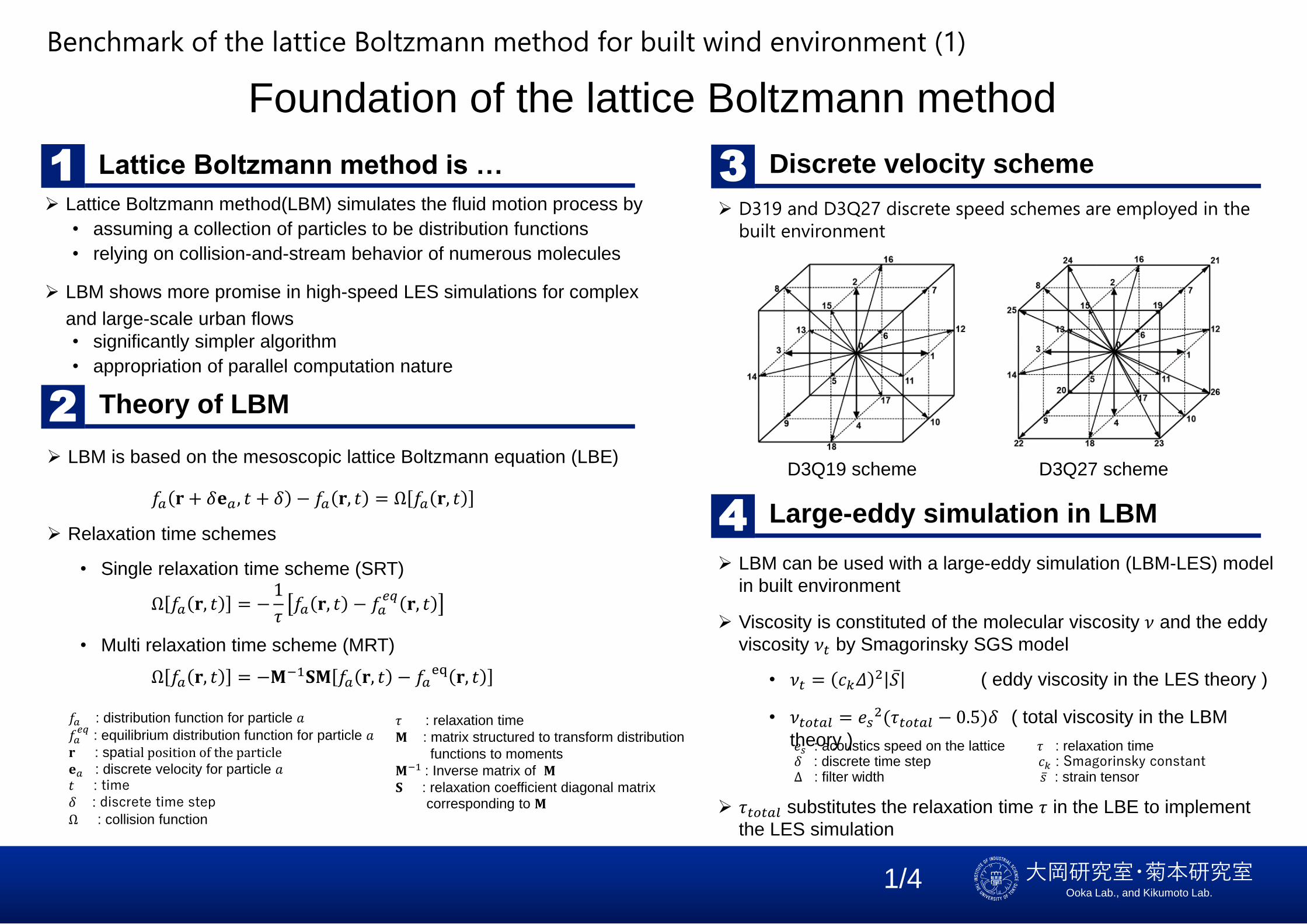
3 Discrete velocity scheme
4 Large-eddy simulation in LBM𝑓𝑎 𝐫 + 𝛿𝐞𝑎 , 𝑡 + 𝛿 − 𝑓𝑎 𝐫, 𝑡 = Ω 𝑓𝑎 𝐫, 𝑡
➢ Lattice Boltzmann method(LBM) simulates the fluid motion process by
• assuming a collection of particles to be distribution functions
• relying on collision-and-stream behavior of numerous molecules
➢ LBM shows more promise in high-speed LES simulations for complex
and large-scale urban flows
• significantly simpler algorithm
• appropriation of parallel computation nature
➢ Relaxation time schemes
Ω 𝑓𝑎 𝐫, 𝑡 = −1
𝜏𝑓𝑎 𝐫, 𝑡 − 𝑓𝑎
𝑒𝑞𝐫, 𝑡
Ω 𝑓𝑎 𝐫, 𝑡 = −𝐌−1𝐒𝐌 𝑓𝑎 𝐫, 𝑡 − 𝑓𝑎eq 𝐫, 𝑡
• Single relaxation time scheme (SRT)
• Multi relaxation time scheme (MRT)
➢ LBM can be used with a large-eddy simulation (LBM-LES) model
in built environment
➢ Viscosity is constituted of the molecular viscosity 𝜈 and the eddy
viscosity 𝜈𝑡 by Smagorinsky SGS model
D3Q19 scheme D3Q27 scheme
• 𝜈𝑡 = 𝑐𝑘𝛥2 ҧ𝑆 ( eddy viscosity in the LES theory )
• 𝜈𝑡𝑜𝑡𝑎𝑙 = 𝑒𝑠2(𝜏𝑡𝑜𝑡𝑎𝑙 − 0.5)𝛿 ( total viscosity in the LBM
theory )𝑒𝑠 : acoustics speed on the lattice 𝜏 : relaxation time𝛿 : discrete time step 𝑐𝑘 : Smagorinsky constantΔ : filter width ҧ𝑠 : strain tensor
𝜏 : relaxation time
𝐌 : matrix structured to transform distribution
functions to moments
𝐌−1 : Inverse matrix of 𝐌𝐒 : relaxation coefficient diagonal matrix
corresponding to 𝐌
➢ D319 and D3Q27 discrete speed schemes are employed in the
built environment
𝑓𝑎 : distribution function for particle 𝑎𝑓𝑎𝑒𝑞
: equilibrium distribution function for particle 𝑎𝐫 : spatial position of the particle𝐞𝑎 : discrete velocity for particle 𝑎𝑡 : time𝛿 : discrete time stepΩ : collision function
大岡研究室・菊本研究室Ooka Lab., and Kikumoto Lab.
Benchmark of the lattice Boltzmann method for built wind environment (2)
Benchmark of LBM for the indoor isolated flow
2/4
LBM-LES FVM-LES
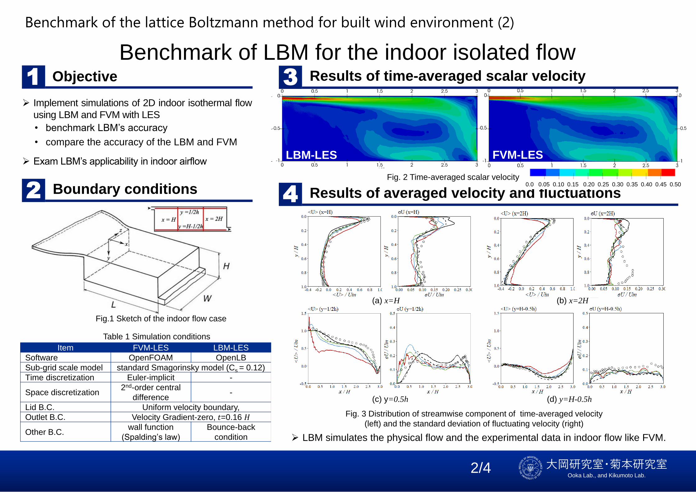
➢ Implement simulations of 2D indoor isothermal flow
using LBM and FVM with LES
• benchmark LBM’s accuracy
• compare the accuracy of the LBM and FVM
➢ Exam LBM’s applicability in indoor airflow
➢ LBM simulates the physical flow and the experimental data in indoor flow like FVM.
Objective1
2 Boundary conditions
3 Results of time-averaged scalar velocity
4 Results of averaged velocity and fluctuations
Item FVM-LES LBM-LES
Software OpenFOAM OpenLB
Sub-grid scale model standard Smagorinsky model (Cs = 0.12)
Time discretization Euler-implicit -
Space discretization2nd-order central
difference-
Lid B.C. Uniform velocity boundary,
Outlet B.C. Velocity Gradient-zero, 𝑡=0.16 𝐻
Other B.C.wall function
(Spalding’s law)
Bounce-back
condition
Table 1 Simulation conditions
Fig.1 Sketch of the indoor flow case
0.0 0.05 0.10 0.15 0.20 0.25 0.30 0.35 0.40 0.45 0.50
(a) x=H (b) x=2H
(c) y=0.5h (d) y=H-0.5h
Fig. 2 Time-averaged scalar velocity
Fig. 3 Distribution of streamwise component of time-averaged velocity
(left) and the standard deviation of fluctuating velocity (right)
大岡研究室・菊本研究室Ooka Lab., and Kikumoto Lab.
Benchmark of the lattice Boltzmann method for built wind environment (3)
Benchmark of LBM for the outdoor isolated flow (part 1)
3/4
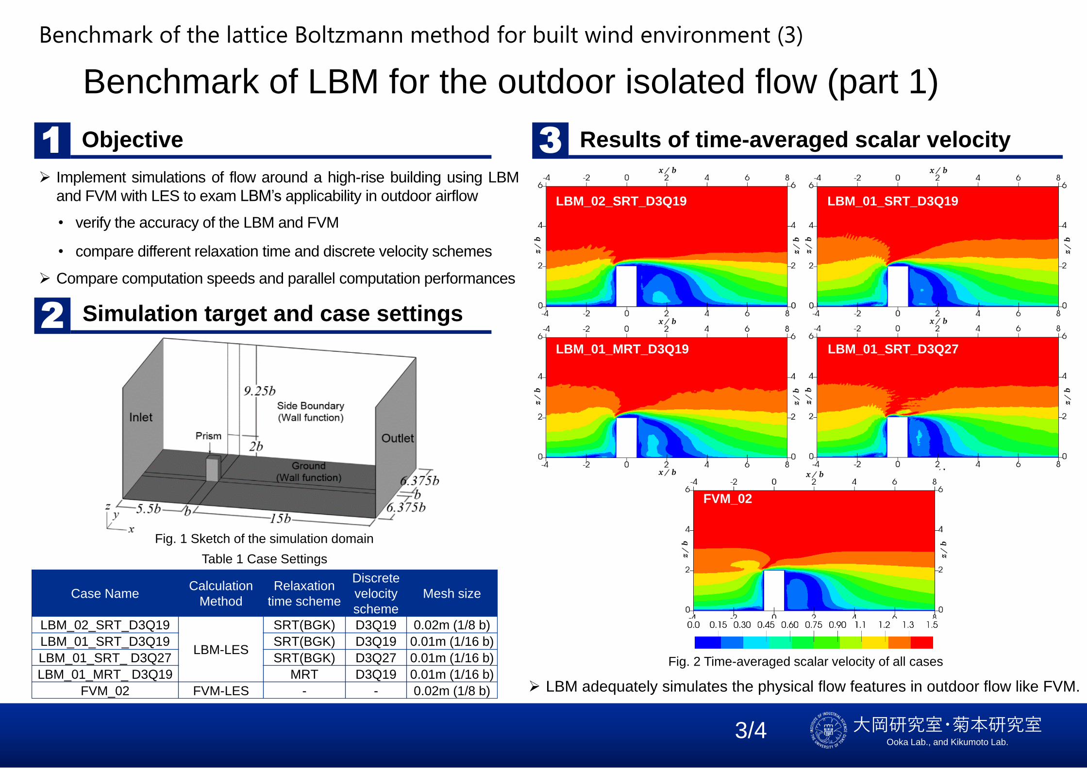
Objective1
2 Simulation target and case settings
Results of time-averaged scalar velocity3
➢ LBM adequately simulates the physical flow features in outdoor flow like FVM.
Table 1 Case Settings
➢ Implement simulations of flow around a high-rise building using LBM
and FVM with LES to exam LBM’s applicability in outdoor airflow
• verify the accuracy of the LBM and FVM
• compare different relaxation time and discrete velocity schemes
➢ Compare computation speeds and parallel computation performances
LBM_02_SRT_D3Q19 LBM_01_SRT_D3Q19
LBM_01_MRT_D3Q19 LBM_01_SRT_D3Q27
FVM_02
Case NameCalculation
Method
Relaxation
time scheme
Discrete
velocity
scheme
Mesh size
LBM_02_SRT_D3Q19
LBM-LES
SRT(BGK) D3Q19 0.02m (1/8 b)
LBM_01_SRT_D3Q19 SRT(BGK) D3Q19 0.01m (1/16 b)
LBM_01_SRT_ D3Q27 SRT(BGK) D3Q27 0.01m (1/16 b)
LBM_01_MRT_ D3Q19 MRT D3Q19 0.01m (1/16 b)
FVM_02 FVM-LES - - 0.02m (1/8 b)
Fig. 1 Sketch of the simulation domain
Fig. 2 Time-averaged scalar velocity of all cases
大岡研究室・菊本研究室Ooka Lab., and Kikumoto Lab.
Benchmark of the lattice Boltzmann method for built wind environment (3)
Benchmark of LBM for the outdoor isolated flow (part 2)
4/4
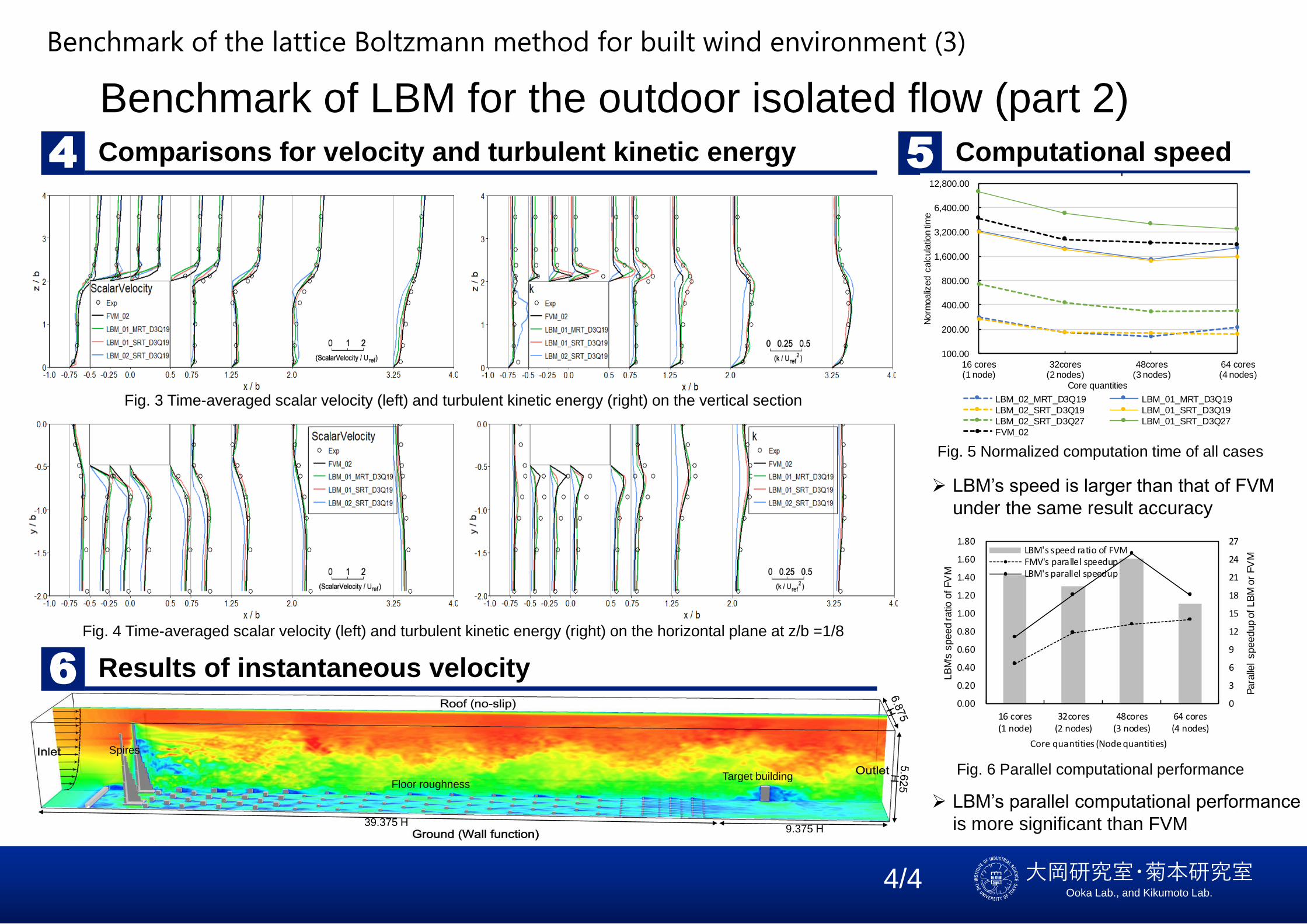
39.375 H9.375 H
Target buildingFloor roughness
Spires
Comparisons for velocity and turbulent kinetic energy4 Computational speed5
0
3
6
9
12
15
18
21
24
27
0.00
0.20
0.40
0.60
0.80
1.00
1.20
1.40
1.60
1.80
16 cores(1 node)
32cores(2 nodes)
48cores(3 nodes)
64 cores(4 nodes)
Para
llel
speedup o
f LB
M o
r FV
M
LB
M's
speed ratio
of FV
M
Core quantities (Node quantities)
Speed ratio and parallel speedup
LBM's speed ratio of FVMFMV's parallel speedupLBM's parallel speedup
100.00
200.00
400.00
800.00
1,600.00
3,200.00
6,400.00
12,800.00
16 cores(1 node)
32cores(2 nodes)
48cores(3 nodes)
64 cores(4 nodes)
Norm
oaliz
ed c
alc
ula
tion ti
me
Core quantities
Normalized Computation time
LBM_02_MRT_D3Q19 LBM_01_MRT_D3Q19
LBM_02_SRT_D3Q19 LBM_01_SRT_D3Q19
LBM_02_SRT_D3Q27 LBM_01_SRT_D3Q27
FVM_02
Results of instantaneous velocity6
➢ LBM’s speed is larger than that of FVM
under the same result accuracy
➢ LBM’s parallel computational performance
is more significant than FVM
Fig. 3 Time-averaged scalar velocity (left) and turbulent kinetic energy (right) on the vertical section
Fig. 4 Time-averaged scalar velocity (left) and turbulent kinetic energy (right) on the horizontal plane at z/b =1/8
Fig. 5 Normalized computation time of all cases
Fig. 6 Parallel computational performance
Recommended