Giulia Colombo*
*Research Fellow at the Centre for European Economic Research (ZEW), Mannheim, Germany
e-mail: [email protected]
The Effects of DR-CAFTA in Nicaragua:
A CGE-Microsimulation Model for
Poverty and Inequality Analysis
Acknowledgments for data providing The author would like to thank Marco Vinicio Sánchez Cantillo (UN-ECLAC, United
Nations, Economic Commission for Latin America and the Caribbean, Social
Development Unit, ECLAC Subregional Headquarters in Mexico, Mexico, D.F) and Rob
Vos (UN-DESA, United Nations, Department of Economic and Social Affairs, Division
of Politics and Development Analysis, and Affiliated Professor of Finance and
Development at the Institute of Social Studies, The Hague), who kindly supplied the
author with the Social Accounting Matrix for Nicaragua for the year 2000, and the
“Instituto Nacional de Estadísticas y Censos” of Nicaragua and The World Bank (Poverty
and Human Resources Development Research Group, LSMS Data) for making the
household survey for Nicaragua (“Encuesta Nacional de Hogares sobre Medición de
Nivel de Vida”, EMNV 2001) available.
The author is the only responsible for all the ideas and results appearing in the paper.
2
Abstract
In this paper, we build a Computable General Equilibrium (CGE)-microsimulation model
for the economy of Nicaragua, following the Top-Down approach (see Bourguignon et
al., 2003), that is, the reform is simulated first at the macro level with the CGE model,
and then it is passed onto the microsimulation model through a vector of changes in some
chosen variables, such as prices, wage rates, and unemployment levels. The main reason
for this choice is that with such an approach, one can develop the two models (CGE and
microsimulation) separately, thus being able to make use of behavioural micro-
econometric equations, which are instead of more difficult introduction into a fully
integrated model. Moreover, the so called top-down approach appears to be particularly
suited to the policy reform we are willing to simulate with the model: the Free Trade
Agreement of Central America with the USA is mainly a macroeconomic reform, which
on the other hand can have important effects on the distribution of income. With such a
model we try to study the possible changes in the distribution of income deriving from
the Free Trade Agreement with USA. Our analysis finds only small changes both in the
main macroeconomic variables and in the distribution of income and poverty indices.
JEL classification: C68, C35, D31
Keywords: CGE models, microsimulation, income distribution.
3
1. Introduction
In the literature that studies income inequality and poverty, we can observe a
recent development of models that link together a macroeconomic model (usually
a CGE model) and a microsimulation model. The reason for this lays in the fact
that poverty and inequality are typically microeconomic issues, while the policy
reforms or the shocks that are commonly simulated have often a strong
macroeconomic impact on the economy under study. Indeed, the main advantage
of linking these two models is that one is able to take into account full agents’
heterogeneity and the complexity of income distribution, while being able at the
same time to consider the macroeconomic effects of the policy reforms.
In this paper, we build a CGE-microsimulation model for the economy of
Nicaragua, following the Top-Down approach (see Bourguignon et al., 2003),
that is, the reform is simulated first at the macro level with the CGE model, and
then it is passed onto the microsimulation model through a vector of changes in
some chosen variables, such as prices, wage rates, and unemployment levels. The
main reason for this choice is that with such an approach, one can develop the two
models (CGE and microsimulation) separately, thus being able to make use of
behavioural micro-econometric equations, which are instead of more difficult
introduction into a fully integrated model (see for instance Cockburn, 2001, and
Cororaton and Cockburn, 2005).
Moreover, the so called top-down approach appears to be particularly suited to
the policy reform we are willing to simulate with the model: the Free Trade
Agreement of Central America with the USA is mainly a macroeconomic reform,
which on the other hand can have important effects on the distribution of income.
The Free Trade Agreement (CAFTA) between the countries of the American
isthmus and the United States was signed in May 2004 (in August the Dominican
Republic joined the Treaty, known from that moment on under the name DR-
CAFTA). The Nicaraguan Congress ratified the Agreement in October 2005, and
it came into force the 1st April 2006.
4

United States are a very important trade partner for Nicaragua. According to
Sánchez and Vos (2005), in 2000 42% of Nicaraguan exports were directed to the
US market, while 22% of Nicaraguan imports came from the USA. The majority
of commercial exchanges between the two countries concerns agricultural
products. The Trade Agreement provides for a gradual reduction of tariff rates on
imports from USA, to be carried on in the first ten years that follow the
introduction of the Treaty. Anyway, for most products the biggest reduction will
be in the first year. On the other side, Nicaraguan exports toward USA will
benefit of gradual increases in the quotas of entry into the US market1.
The introduction of DR-CAFTA in Nicaragua was controversial. The promoters
of the Agreement claimed an improvement in competitiveness and efficiency in
production, and also new investment in advanced technology by USA was
expected2. On the other side, the opposers of the DR-CAFTA are afraid that it
will bring about a high number of losers, especially among those working in the
traditional sectors, such as the agricultural sector and the small enterprises, which
will not be able to compete with the US producers.
As our model is only a one-country study, we are not going to model the changes
in the regime adopted in USA with respect to goods and commodities coming
from Nicaragua, as well as we will not take into consideration the quotas imposed
on imports from USA, but only the changes in the tariff rates raised on the
imported goods from USA. With such a model we try to study the possible
changes in the distribution of income deriving from the Free Trade Agreement
with the USA. The core of the microsimulation model follows the discrete choice
labour supply approach, and it is based on a multinomial logit specification, while
the CGE model is basically a standard one.
The rest of the paper is organized as follows. Section two describes the model in
detail, for each of its modules: the microsimulation and the CGE models, and how
1 For a more detailed description of the new trade regulation enforced with the DR-CAFTA, see
Sánchez and Vos (2006). 2 The largest US investments in Nicaragua are in the energy, communications, manufacturing,
fisheries, and shrimp farming sectors.
5
the two models are linked together. The third section deals with the results of the
simulation, and section four concludes.
Nicaraguan Economy
Nicaragua is one of the poorest countries in the Latin America and the Caribbean
region. Almost half of Nicaraguan population lives under the poverty line, while
more than 25% of people in the rural areas are extremely poor3. The distribution
of income shows a Gini index which is estimated to be 43.1 (World Bank, 2006)
when computed on consumption, and 57.9 (ECLAC estimate, 2006) when
computed on income.
Agriculture employs about 30% of the workforce and accounts for about one fifth
of the gross domestic product. The main commercial crops are coffee, cotton, and
sugarcane; these, together with meat, are the largest exports.
During the 1980s Nicaragua's economy underwent a strong recession, due both to
the civil war, which caused the destruction of much of the country's
infrastructure, and to the economic blockade staged by the USA from 1985
onwards.
At the beginning of the 1990s began a significant process toward macroeconomic
stabilization. Pacification, international aid, continued foreign investment and the
re-establishing of trading relationships with US have contributed to the
stabilization process. Moreover, important trade reforms were carried over in
those years: most of the quantitative restrictions to imports and exports were
3 Around 46% of the population lives below the poverty line established by the 2001 Living
Standards Measurement Survey and 15% of the population lives in extreme poverty (The World
Bank, 2003). These indicators are even higher according to other estimates, such as those
contained in the Statistical Yearbook published by the Economic Commission for Latin America
and the Caribbean (ECLAC, 2006). The differences in the estimates come from different levels of
the poverty line, and from the different reference variable adopted (consumption or income).
6
removed, and there was a net reduction of tariffs on imports, together with a
liberalization of the financial sector.
At the end of the 1990s the economy suffered a slowdown, due to the financing of
the reconstruction after the damage caused by Hurricane Mitch in the fall of 1998,
and to a simultaneous fall in the price of coffee and an increase in the price of oil.
Nicaragua continues to be dependent on international aid and debt relief under the
Heavily Indebted Poor Countries (HIPC) initiative.
2. The Model
2.1. The Microsimulation Model
The main role of the microsimulation module in the linked framework is to
provide a detailed computation of net incomes at the household level, through a
detailed description of the tax-benefit system of the economy, and to estimate
individual behavioural responses to the policy change.
The data source for the building and estimation of the microsimulation model is
the “Encuesta Nacional de Hogares sobre Medición de Nivel de Vida” (EMNV)
of 2001, supplied by the Instituto Nacional de Estadísticas y Censos and The
World Bank (Poverty and Human Resources Development Research Group,
LSMS Data).
The survey includes information regarding income and expenditures of 4191
families, in which live 22810 individuals. Of these individuals, 12645 are at
working age (15-65). Moreover, we have information on 2079 non agricultural
activities and 1547 farm activities.
7
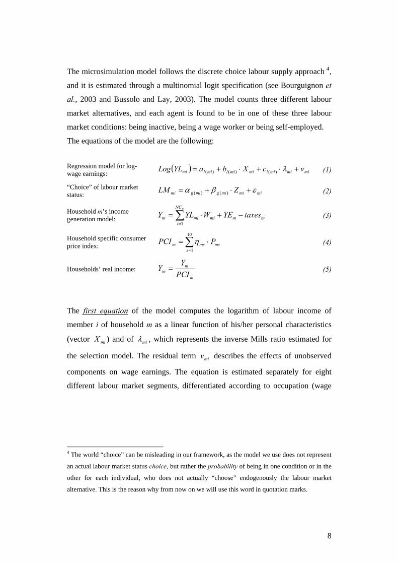
The microsimulation model follows the discrete choice labour supply approach 4,
and it is estimated through a multinomial logit specification (see Bourguignon et
al., 2003 and Bussolo and Lay, 2003). The model counts three different labour
market alternatives, and each agent is found to be in one of these three labour
market conditions: being inactive, being a wage worker or being self-employed.
The equations of the model are the following:
Regression model for log-wage earnings:
( ) mimimilmimilmilmi vcXbaYLLog +⋅+⋅+= λ)()()( (1)
“Choice” of labour market status: mimimigmigmi ZLM εβα +⋅+= )()( (2)
Household m’s income generation model: mm
NC
imimim taxesYEWYLY
m
−+⋅= ∑=1
(3)
Household specific consumer price index: ∑
=
⋅=10
1smsmsm PPCI η (4)
Households’ real income: m
mm PCI
YY = (5)
The first equation of the model computes the logarithm of labour income of
member i of household m as a linear function of his/her personal characteristics
(vector ) and of miX miλ , which represents the inverse Mills ratio estimated for
the selection model. The residual term describes the effects of unobserved
components on wage earnings. The equation is estimated separately for eight
different labour market segments, differentiated according to occupation (wage
miv
4 The world “choice” can be misleading in our framework, as the model we use does not represent
an actual labour market status choice, but rather the probability of being in one condition or in the
other for each individual, who does not actually “choose” endogenously the labour market
alternative. This is the reason why from now on we will use this word in quotation marks.
8
worker or self-employed), gender and skill level. The index function l(mi) assigns
individual i of household m to a specific labour market segment5.
The second equation represents the “choice” of labour status made by household
members. Each individual at working age has to “choose” among three
alternatives: being a wage worker, being self-employed or being inactive. We
estimate the selection model using a multinomial logit specification, which
assigns each individual to the alternative with the highest associated probability.
In our model we have arbitrarily set to zero the utility of being inactive. Vector
of explanatory variables includes some personal characteristics of individual i
of household m. The equation is defined only for individuals at working age, and
it is estimated separately for different demographic groups, defined for household
heads, spouses and other members. The index function g(mi) assigns each
individual to a specific demographic group.
miZ
The third equation is an accounting identity that defines total household net
income, Ym, as the sum of the labour income of its members YLmi (NCm is the
number of members at working age in household m) and of the exogenous income
YEm, net of taxes. The variable is a dummy variable taking value one if
individual i of household m is a wage worker, and zero otherwise. Taxes on
income are computed according to “Ley de equidad fiscal”, which was introduced
in 2003.
miW
Real net income in equation (5) is computed dividing nominal household income
by a household specific consumer price index, as computed in equation (4), where
msη are consumption shares for different goods and Ps is the price of good s.
We have grouped the various commodities into 10 consumption goods.
5 In the original model implemented in Bourguignon et al. (2003) there is a specific equation
which estimates family income deriving from self-employment activity on the base of household’s
characteristics. In the present work we have instead the income declared by self-employed as
labour income, and we do not need an additional equation to compute the income deriving from
self-employment activity.
9

Estimation
The aim of the first equation in the model is to obtain efficient estimates for
labour incomes and incomes deriving from self-employment activity, but only for
those individuals that are observed to be inactive in the survey. These estimates
are used in the case that, after a policy reform, one or more of them will change
their labour market status and become wage workers or go into self-employment
activity. In this case, using these estimates, we will be able to assign a wage or a
labour income to individuals that have changed their labour market status after the
simulation run.
For all the other individuals that are observed to receive a wage or to earn a
positive income from their activity, we use instead the observed wage and income
levels and not the estimated ones.
Equation (1) is estimated separately for each labour market segment, which is
defined according to occupation, gender and skill level. An individual is
considered high-skilled when his/her education attainment is more than primary
school, and unskilled otherwise. We estimated the equation using a Heckman
two-step procedure to correct for the selection bias6. Vector includes some
regional dummies, the logarithm of age, and the number of school years attended.
In the selection equation we used a dummy indicating the presence or not of
children under six, a dummy variable indicating the racial group (distinguished in
white and non-white), and the number of adults living in the household to correct
for the selection bias. The estimation results for the labour market segments low-
skilled wage workers, women, and high-skilled self-employed, men, are reported
in Appendix, Tables 1A and 2A.
miX
Equation (2) represents the “choice” of the labour status made by individuals.
Each individual can “choose” among three alternatives: being inactive, being a
wage worker or being self-employed. The utility of being inactive is arbitrarily set
to zero. Parameters of this equation were obtained through the estimation of a
6 Inactive people are divided only according to gender and skill level.
10
multinomial logit model, assuming that the residual terms iε are distributed
according to the Extreme Value Distribution – Type I7. The estimation was
conducted on sub-samples of individuals at working age, differentiated according
to their demographic group (household heads, spouses, and other members). The
explanatory variables include some regional dummies, sex, logarithm of age, skill
level, illiteracy and racial group, the number of household members and that of
children under six. For spouses and other members we also used labour market
status, skill level and illiteracy of the household head. The model is estimated by
Maximum Likelihood. The estimation results are reported in Appendix, Tables
3A to 5A.
Following the procedure described in Duncan and Weeks (1998), we drew a set of
error terms iε for each individual from the extreme value distribution, in order to
obtain for each individual an estimate that is consistent with his/her observed
activity or inactivity status. From these drawn values, we selected 100 error terms
for each individual, in such a way that, when adding it to the deterministic part of
the model, it perfectly predicts the activity status that is observed in the survey.
After a policy change, only the deterministic part of the model is recomputed.
Then, by adding the random error terms previously drawn to the recomputed
deterministic component, a probability distribution over the three alternatives
(being a wage worker, being self-employed or being inactive) is generated for
each individual. This implies that the model does not assign every individual from
the sample to one particular alternative, but it gives the individual probabilities of
being in one condition rather than in the other. This way, the model does not
7 The Extreme Value distribution (Type I) is also known as Gumbel (from the name of the
statistician who first studied it) or double exponential distribution, and it is a special case of the
Fisher-Tippett distribution. It can take two forms: one is based on the smallest extreme and the
other on the largest. We will focus on the latter, which is the one of interest for us. The standard
Gumbel distribution function (maximum) has the following probability and cumulative density
functions, respectively:
pdf: ( )xexxf −−−= exp)(
CDF: ( )xexF −−= exp)( .
11
identify a particular labour market status for each individual after the policy
change, but generates a probability distribution over the different alternatives8.
2.2. The CGE Model
The main characteristics of the CGE model are the following.
There are two representative households, divided according to their residence in
urban or rural areas. Both maximize utility according to a Linear Expenditure
System (LES) system. They obtain income from their supply of labour and
capital, and they also receive transfers from the government and remittances from
abroad.
Domestic production is carried on by 38 production sectors, which are producing
38 commodities following a Leontief technology in the aggregation of value
added (capital and aggregate labour) and the intermediate aggregate. The
aggregation of intermediate inputs is done according to a Leontief technology,
while capital and labour are aggregated into value added according to a Constant
Elasticity of Substitution (CES) function.
Labour demand is divided into eight different labour types, distinguished
according to sex, qualification level and occupation (wage workers or self-
employed) of the workers. These labour types are then aggregated to form a
“labour aggregate” according to a CES function. The price of each labour type is
set at the level of its marginal productivity.
Investments in the economy are savings-driven.
The public sector consumes goods, saves, and raises taxes on households’
income, on firms’ output and sells, on consumption of certain goods and tariffs on
imports. It also pays subsidies to exports, and transfers to firms and households.
8 This procedure is also described in Creedy and Kalb (2005). See also Creedy et al. (2002b).
12
The equilibrium of public budget constraint is reached through the change in
public savings.
For the foreign sector the Armington assumption holds, and domestic production
and imports are aggregated through a CES function. Domestic production is
divided into supply of exports and supply of domestically produced good for the
internal market following a Constant Elasticity of Transformation (CET) function.
A stylized scheme of the production structure and of the foreign sector design is
reported in Appendix B.
Calibration
The calibration of the model is done on the Social Accounting Matrix (SAM) for
Nicaragua for the year 2000 (see Sánchez and Vos, 2005 for details).
Some parameter values were taken from the existing literature. Sánchez and Vos
(2005) is the source for the values of the substitution elasticities in the production
function, in the Armington function (aggregation of the composite good sold on
the internal market), and in the CET function (aggregation of internal production
intended to the internal market and exports)9. Sánchez and Vos (2005) also
estimated the values of income elasticity of consumption demand using the data
of the EMNV 2001. The values for the Frisch parameter were taken from Lluch,
Powell and Williams (1977).
For what concerns the elasticity of substitution among the eight different labour
types, we implemented a sensitivity analysis, using different values of elasticity.
We report the results of the simulation for the different values considered in this
sensitivity analysis (see Appendix C).
13
2.3. Linking The Two Models
The basic difficulty of the Top-Down approach is to ensure consistency between
the micro and macro levels of analysis. Thus, it is necessary to introduce a system
of equations to ensure the achievement of consistency between the two models10.
In practice, this consists in imposing the macro results obtained with the CGE
model onto the microeconomic level of analysis. In particular, the changes in the
commodity prices, Pq, must be equal to those resulting from the CGE model; the
changes in average earnings with respect to the benchmark in the micro-
simulation module must be equal to the changes in the wage rate obtained with
the CGE model, as well as the change in the return to capital in the micro-
simulation module must be equal to the one observed after the simulation run in
the CGE model. In addition, the changes in the number of wage workers in the
micro-simulation model must match those observed in the CGE model.
In our model, these consistency conditions translate into the following set of
constraints, which can be called “linking” equations:
Household specific consumer price index: ( CGE
s
NG
smsmsm PPPCI Δ+⋅⋅= ∑
=
11η ) (L.1)
Logarithm of wage earnings: ( ) ( )[ ]CGEmimi PLLYLogYLLog Δ+⋅= 1ˆ (L.2)
Capital income: ( )CGEmm PKKSYK Δ+⋅= 1 (L.3)
Employment level: CGEl
MSl EMPEMP Δ=Δ (L.4)
The variables with no superscripts are those coming from the microsimulation
module; those with the ^ notation correspond to the ones that have been
9 Sánchez and Vos (2005) used the values estimated in Sánchez (2004) for a similar model for
Costa Rica, carrying on a sensitivity analysis for some parameter values. 10 This way, what happens in the MS module can be made consistent with the CGE modelling by
adjusting parameters in the MS model, but, from a theoretical point of view, it would be more
satisfying to obtain consistency by modelling behaviour identically in the two models.
14
estimated: in particular, is the wage level resulting from the regression
model for individual i, member of household m, while is the labour market
status of individual i of household m deriving from the estimation of the
multinomial model.
)ˆ( miLYLog
miW
CGEsPΔ , and CGEPLΔ CGEPKΔ indicate, respectively, the change in the prices of
goods, the change in the wage rate and in the return to capital deriving from the
simulation run of the CGE model, while and are the
employment level percentage changes for the CGE model and the
microsimulation model for labour type l.
CGElEMPΔ MS
lEMPΔ
From equation (L.4), the number of newly employed (or inactive) of labour type l
resulting from the MS model must be equal to the change in the employment level
of labour type l observed after the CGE run. This implies that the CGE model
determines the employment level of the economy after the simulation, and that
the MS model selects which individuals among the inactive persons have the
highest probability of becoming employed (if the employment level is increased
from the CGE simulation result), or either who, among the wage workers or self-
employed, has the lowest probability of being employed after the policy change
(if the employment level is decreased)11.
One possible way of imposing the equality between the two sets of parameters of
system of equations (L) is through a change in the parameters of the selection and
regression models. Following Bourguignon et al. (2003), we restrict this change
in the parameters to a change in the intercepts of functions (1) and (2). The
justification for this choice is that it implies a neutrality of the changes, that is,
changing the intercepts a of equation (1) just shifts proportionally the estimated
labour income of all individuals, without causing any change in the ranking
between one individual and the other. The same applies for the labour market
status selection equation: we choose to change the intercept α of equation (2), and
11 And, in this case, his/her new wage level will be determined by the regression model of wage
earnings.
15
this will shift proportionally all the individual probabilities of each alternative,
without changing their relative positions in the probability distribution, only to let
some more individuals become employed (or some less if the employment rate of
the CGE model is decreased), irrespectively of their personal characteristics. This
change in the intercept will be of the amount that is necessary to reach the number
of wage workers or self-employed resulting from the CGE model. Thus, this
choice preserves the ranking of individuals according to their ex-ante probability
of being employed, which was previously determined by the estimation of the
multinomial model. For this reason the change in the intercept parameter satisfies
this neutrality property.
3. Simulation
The simulation of the introduction of DR-CAFTA into the Nicaraguan economy
consists of a reduction of tariff rates on imports from the US.
As we are working with a static model, we cannot model the scheduled gradual
change in the tariff rates, which is planned to be distributed along the ten years
following the introduction of the Trade Agreement. As our model does not have
any dynamic characteristic, it will be able capture the effects of the Treaty in the
short-medium run, say about five years. Thus, the simulation we implemented
will take into account the reduction in the tariff rates which is intended to take
place after the first five years of effectiveness of the Treaty. This choice is
expected to have no big influence on the results of the model, as the main tariff
reduction for most of the commodities will take place in the first year after the
introduction of the Agreement.
As our model is only a one-country study, we are not going to model the changes
in the regime adopted in USA with respect to goods and commodities imported
from Nicaragua. So, for instance, we are not going to take into account the access
quotas imposed on these imports from Nicaragua to USA. These quotas are
16

represented by limits to the importable quantities of some goods (in particular,
beef, peanuts, cheese and sugar), but they are planned to reach an unlimited
amount for beef and peanuts after the fifteenth year of enforcement of the Treaty,
while for cheese they will be more than doubled after sixteen years. The unique
quota which is expected to remain quite low is the one imposed on sugar, which
will reach an amount 30% superior than the one imposed in the first year of
enforcement of the Agreement.
The general reduction in the first five years after the introduction of the Treaty is
about thirty percent of the previously adopted tariffs. The reductions adopted for
the specific commodities and services are reported in Table 1C.
As the supporters of the agreement with US expected an increase in the capital
investments from USA in Nicaragua, we also considered an exogenous change in
the initial capital endowment of different amounts (2, 5 and 10 %, respectively).
The percentage changes resulting from the simulation for a selected set of
variables are reported in Appendix C, Tables 2C-13C.
A sensitivity analysis was also conducted to take into account different possible
values for the elasticity of substitution of labour demand at the stage of
aggregation of the eight different types of labour, which are divided according to
sex, qualification level and occupation (wage workers or self-employed) of the
workers, as explained in the description of the CGE model.
The results show a very little answer of the economy to the tariff change. This
outcome is not completely surprising, because the tariff levels which were in
force previous the introduction of the DR-CAFTA were already quite low.
Moreover, other studies found not only for Nicaragua but also for other countries
in the region the same small answer to trade liberalization12.
The sole reduction of tariffs on imports will cause a very small increase in total
domestic production which in the best hypothesis will be of 0.2 %. However, if
12 See for instance Sánchez (2005), Vos et al. (2004), and the book edited by Ganuza et al. (2004),
which contains sixteen country-studies on different countries in Latin and Central America on the
consequences of the trade liberalization carried on during the last decades in this region.
17
we consider a small value for the elasticity of substitution among different labour
inputs (elasticity fixed at 0.3), the change in domestic output is even negative.
The negative response of output in this case is alleviated when considering a
positive shock in the initial capital endowment, but this shock has to be of
significant amount to cause a positive change in output (10% change in capital
endowment).
However, if we try to have a closer look to the sectoral effects of the reform (see
Tables 3C, 6C and 9C), and considering only the tariff reduction, we can observe
that traditional sectors such as the agricultural and textile sectors are increasing
their production, while the capital intensive (industrial sectors) sectors lose. On
the contrary, when we take into account also the capital shock (simulations 2, 3
and 4), the direction of these results is inverted, so that we have the capital
intensive sectors gaining and the traditional sectors (agricultural and textile
sectors) that decrease their production level.
In all cases, however, the overall increase in production seems to be driven by the
growth of the exporting sectors, which are gaining in all the simulations.
Anyway, the reduction of the tariff rates on imports does not generate significant
losses for the government, as tax revenues do not decrease of high amounts.
When the elasticity of substitution for labour is considered at the same level of the
one used for value added aggregation, tax revenues even increase, due to the
higher production and consumption levels in the economy. This increase becomes
even bigger when we introduce a positive shock to capital endowment.
Taking into consideration the positive shock to capital endowment, the changes
considered are in general of a higher amount, but anyway in the best hypothesis
of a 10% change in the capital stock, the resulting change in domestic production
will be around 1.5%.
In the first scenario (reduction of tariff rates on imports only), the change in
labour demand apparently favours unskilled workers, and women in particular,
except for the case with a low elasticity of substitution, where a small increase in
the demand for qualified workers is experienced. The change in the employment
levels of wage workers and self-employed depends similarly on the adopted value
18
of the elasticity of substitution. Anyway, all the changes occurring in the
employment levels of the different labour inputs are very small.
When the elasticity of substitution is sufficiently high (higher than 0.3), real wage
is observed to increase, as well as real income does, thus increasing consumption
levels for both rural and urban households.
For what concerns the microeconomic results, that is the changes in income
distribution and poverty, we can observe in general very small changes in the
underlying indices.
Taking into account only the reduction in tariffs on imports, poverty rates at a
national level decrease in all the counterfactuals. On the contrary, income
inequality is rising (even if of a very little amount), especially when we consider
separated indices for urban and rural areas. Poverty seems to decrease more in
urban than in rural areas.
This result of an increasing income inequality in both urban and rural areas
confirms what was already found by Vos et al. (2004) for most of Latin and
Central American countries in the case of trade liberalization.
When we take into account the positive shock on capital, then income inequality
is observed to decrease. Anyway, the negative changes resulting in both income
inequality and poverty indices remain very small (and in some cases they are even
positive, such as in the case with constant elasticity of substitution in labour
inputs equal to the elasticities used in value added aggregation), and especially in
rural areas, where poverty is observed to have its greatest incidence.
19
4. Conclusion
The small positive results deriving from our analysis show that the introduction of
the Free Trade Agreement with US in Nicaragua cannot be seen as the unique
solution to the high poverty rates and the unequal income distribution of the
country. In the best hypothesis the consequent increment in production would be
of around 1.5%. This result is not surprising, as the tariff levels in force before the
introduction of the DR-CAFTA were already quite low, after the process of trade
liberalization carried on during the 1990s in all Central and Latin America’s
countries.
The main impact of the Treaty is to be found in the increase of exports, which,
according to the supporters of the Agreement, are expected to be the leading
engine of future development and economic growth in the country. Anyway, this
increment in the amount of exported good is able to increase domestic production
of only 1.5 percentage points in the best scenario.
It is true however that in our model we did not take into account the possible
improvement in productivity generated by the new investments in advanced
technology coming from the US, which could have given a major boost to the
economy. Anyway, the dynamic model developed by Sánchez and Vos (2006),
which includes also a positive shock on factor productivity, finds again small
responses of the economy to trade liberalization, and to the Trade Agreement with
the USA in particular.
The DR-CAFTA alone seems to be unable to bring about big changes in the
structure of the economy, and especially for what concerns poverty and inequality
reduction. It should at least be accompanied by other policies supporting lower
incomes, especially in rural areas. One possible future implementation of the
model presented here could be the design and the analysis of such a policy.
20
References Armington P.S. (1969), A Theory of Demand for Products Distinguished by Place of Production, IMF Staff Paper n° 16, pp.159-176. Arntz, M., Boeters S., Gürtzgen N., Schubert S. (2006), Analysing Welfare Reform in a Microsimulation-AGE Model: The Value of Disaggregation, ZEW Discussion Paper No. 06-076, Mannheim. Bussolo M. and Lay J. (2003), Globalisation and Poverty Changes: A Case Study on Colombia, Working Paper No. 226, OECD Development Centre, Paris. Bourguignon F., Robilliard A.S. and Robinson S. (2003), Representative versus real households in the macro-economic modelling of inequality, Document de travail DIAL/Unité de recherche CIPRE. Cockburn J. (2001), Trade Liberalization and Poverty in Nepal: A Computable General Equilibrium Micro-simulation Approach. Working Paper 01-18, CRÉFA, Université Laval. Cororaton C.B., Cockburn J. (2005), Trade Reform and Poverty in the Philippines: a Computable General Equilibrium Microsimulation Analysis, CIRPÉE, Working Paper 05-13, Université Laval. Creedy J. and Kalb G. (2005), Discrete hours labour supply modelling: specification, estimation and simulation, Journal of Economic Surveys 19, 697-734. Creedy J., Duncan A. (2002a), Behavioural Microsimulation with Labour Supply Responses, Journal of Economic Surveys n. 16, pp. 1-38. Creedy J., Duncan A., Harris M. and Scutella R. (2002b), Microsimulation Modelling of Taxation and The Labour Market: The Melbourne Institute Tax Transfer Simulator, Cheltenham: Edward Elgar. Davies J.B. (2004), Microsimulation, CGE and Macro Modelling for Transition and Developing Economies, WIDER Discussion Paper No. 2004/08. ECLAC (2006), Statistical Yearbook for Latin America and the Caribbean 2006, Santiago: ECLAC-United Nations. Ganuza E., Morley S., Robinson S., Vos R. (eds.) (2004), ¿Quién se beneficia del libre commercio? Promoción de exportaciones y pobreza en América Latina y el Caribe en los 90, Bogotá, PNUD-AlfaOmega. Hérault N. (2005), A Micro-Macro Model for South Africa: Building and Linking a Microsimulation Model to a CGE Model, Melbourne Institute Working Paper Series, WP No. 16/05.
21
Instituto Nacional de Estadísticas y Censos de Nicaragua and The World Bank (Poverty and Human Resources Development Research Group, LSMS Data), Encuesta Nacional de Hogares sobre Medición de Nivel de Vida, 2001 Lluch C., A.A. Powell and R. Williams (1977), Patterns in Household Demand and Saving, London: Oxford University Press. Sánchez C., M.V. (2004), Rising inequality and falling poverty in Costa Rica’s agriculture during trade reform. A macro-micro general equilibrium analysis. Maastricht: Shaker. Sánchez C., M.V. (2005), Reformas económicas, régimen cambiario y choques externos : efectos en el desarrollo económico, la disegualdad y la pobreza en Costa Rica, El Salvador y Honduras, Serie de Estudio y Perspectivas, N° 36, Sede Subregional CEPAL en Mexico. Sánchez C., M.V. and R. Vos (2005), Impacto del CAFTA en el Crecimiento, la Pobreza y la Disegualidad en Nicaragua. Una evaluación ex-ante con un modelo de equilibrio general computable dinámico. Informe Final, New York and Mexico City, December 2005. Sánchez C., M.V. and R. Vos (2006), DR-CAFTA: ¿panacea o fatalidad para el desarrollo económico y social en Nicaragua?, CEPAL, Serie Estudios y Perspectivas N° 57, Sede Subregional de la CEPAL en México. Savard L. (2003), Poverty and Income Distribution in A CGE-Household Micro-Simulation Model: Top-Down/Bottom-Up Approach, CIRPÉE Working Paper 03-43, Université Laval. The World Bank (2003), Nicaragua, Reporte de Pobreza. Documento del Banco Mundial. Departamento de Centro América, Región de América Latina y el Caribe. Informe No. 26128-NI. The World Bank (2006), Human Development Report 2006, Published for the United Nations Development Programme (UNDP): New York. Vos R., Ganuza E., Morley S., Robinson S., Pineiro V. (2004), Are Export Promotion and Trade Liberalization Good for Latin America’s poor ? A Comparative Macro-Micro CGE Analysis, Institute of Social Studies, Working Paper Series No. 399, The Hague.
22
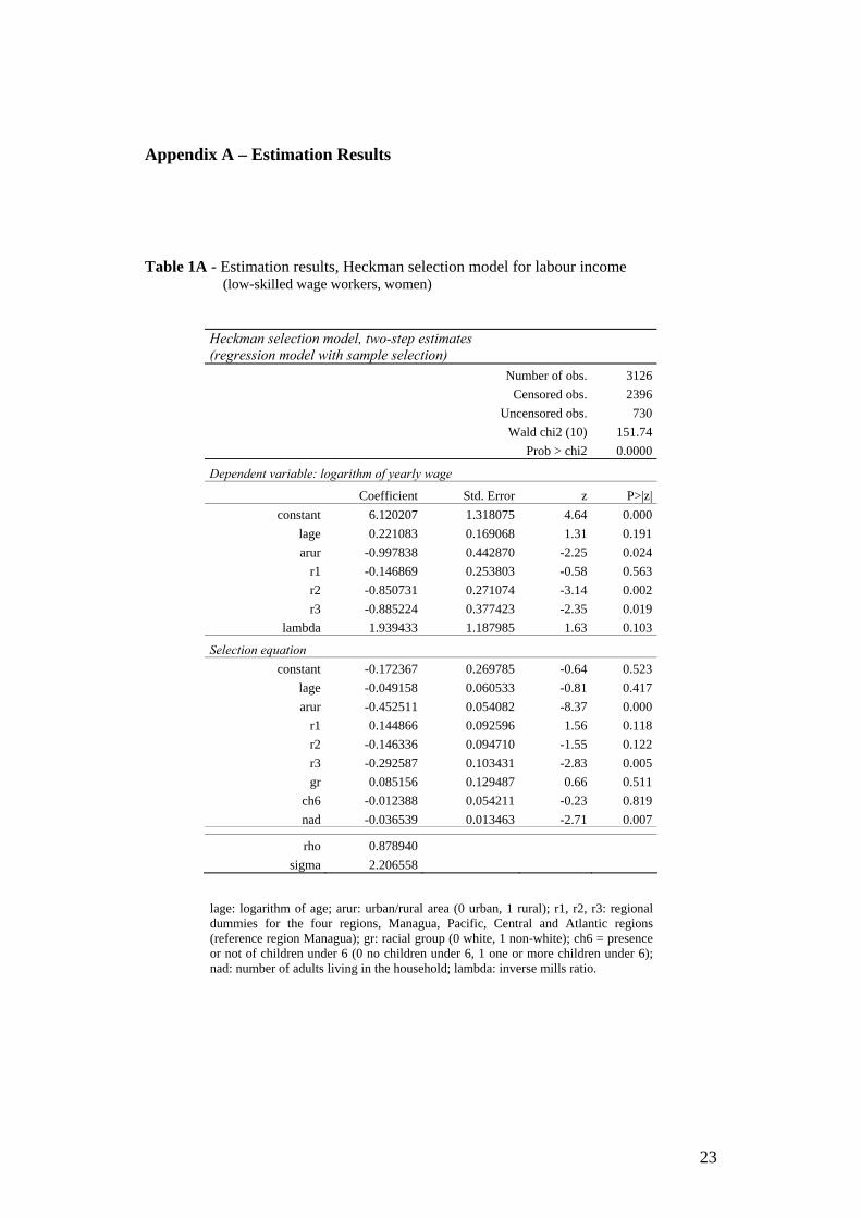
Appendix A – Estimation Results Table 1A - Estimation results, Heckman selection model for labour income
(low-skilled wage workers, women)
Heckman selection model, two-step estimates (regression model with sample selection)
Number of obs. 3126 Censored obs. 2396
Uncensored obs. 730 Wald chi2 (10) 151.74
Prob > chi2 0.0000
Dependent variable: logarithm of yearly wage Coefficient Std. Error z P>|z|
constant 6.120207 1.318075 4.64 0.000 lage 0.221083 0.169068 1.31 0.191 arur -0.997838 0.442870 -2.25 0.024
r1 -0.146869 0.253803 -0.58 0.563 r2 -0.850731 0.271074 -3.14 0.002 r3 -0.885224 0.377423 -2.35 0.019
lambda 1.939433 1.187985 1.63 0.103
Selection equation constant -0.172367 0.269785 -0.64 0.523
lage -0.049158 0.060533 -0.81 0.417 arur -0.452511 0.054082 -8.37 0.000
r1 0.144866 0.092596 1.56 0.118 r2 -0.146336 0.094710 -1.55 0.122 r3 -0.292587 0.103431 -2.83 0.005 gr 0.085156 0.129487 0.66 0.511
ch6 -0.012388 0.054211 -0.23 0.819 nad -0.036539 0.013463 -2.71 0.007
rho 0.878940 sigma 2.206558
lage: logarithm of age; arur: urban/rural area (0 urban, 1 rural); r1, r2, r3: regional dummies for the four regions, Managua, Pacific, Central and Atlantic regions (reference region Managua); gr: racial group (0 white, 1 non-white); ch6 = presence or not of children under 6 (0 no children under 6, 1 one or more children under 6); nad: number of adults living in the household; lambda: inverse mills ratio.
23
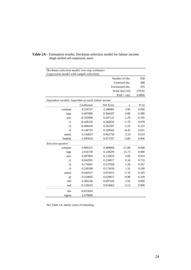
Table 2A - Estimation results, Heckman selection model for labour income
(high-skilled self-employed, men)
Heckman selection model, two-step estimates (regression model with sample selection)
Number of obs. 958 Censored obs. 488
Uncensored obs. 470 Wald chi2 (10) 270.65
Prob > chi2 0.0000
Dependent variable: logarithm of yearly labour income Coefficient Std. Error z P>|z|
constant 8.314737 2.186083 3.80 0.000 lage 0.497086 0.566287 0.88 0.380 arur -0.319998 0.247125 -1.29 0.195
r1 -0.428120 0.242832 -1.76 0.078 r2 -0.406418 0.262587 -1.55 0.122 r3 -0.148755 0.328582 -0.45 0.651
annist 0.134023 0.062750 2.14 0.033 lambda -1.695824 0.471557 -3.60 0.000
Selection equation constant -5.800225 0.488066 -11.88 0.000
lage 2.016758 0.128209 15.73 0.000 arur 0.007804 0.132835 0.06 0.953
r1 0.042955 0.126017 0.34 0.733 r2 0.174041 0.137928 1.26 0.207 r3 0.230188 0.175659 1.31 0.190
annist -0.044537 0.033413 -1.33 0.183 gr -0.224695 0.229871 -0.98 0.328
ch6 0.384146 0.097169 3.95 0.000 nad -0.126610 0.024663 -5.13 0.000
rho -0.815810 sigma 2.078696
See Table 1A; annist: years of schooling.
24
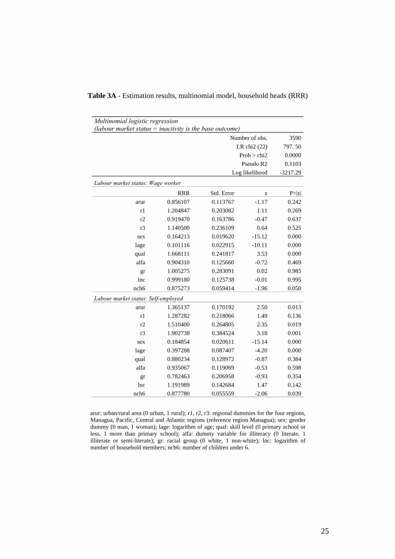
Table 3A - Estimation results, multinomial model, household heads (RRR)
Multinomial logistic regression (labour market status = inactivity is the base outcome)
Number of obs. 3590 LR chi2 (22) 797. 50 Prob > chi2 0.0000 Pseudo R2 0.1103
Log likelihood -3217.29
Labour market status: Wage worker RRR Std. Error z P>|z|
arur 0.856107 0.113767 -1.17 0.242 r1 1.204847 0.203082 1.11 0.269 r2 0.919470 0.163786 -0.47 0.637 r3 1.140500 0.236109 0.64 0.525
sex 0.164213 0.019620 -15.12 0.000 lage 0.101116 0.022915 -10.11 0.000 qual 1.668111 0.241817 3.53 0.000 alfa 0.904310 0.125660 -0.72 0.469
gr 1.005275 0.283091 0.02 0.985 lnc 0.999180 0.125738 -0.01 0.995
nch6 0.875273 0.059414 -1.96 0.050
Labour market status: Self-employed arur 1.365137 0.170192 2.50 0.013
r1 1.287282 0.218066 1.49 0.136 r2 1.510400 0.264805 2.35 0.019 r3 1.902738 0.384524 3.18 0.001
sex 0.184854 0.020611 -15.14 0.000 lage 0.397288 0.087407 -4.20 0.000 qual 0.880234 0.128972 -0.87 0.384 alfa 0.935067 0.119069 -0.53 0.598
gr 0.782463 0.206958 -0.93 0.354 lnc 1.191989 0.142684 1.47 0.142
nch6 0.877780 0.055559 -2.06 0.039
arur: urban/rural area (0 urban, 1 rural); r1, r2, r3: regional dummies for the four regions, Managua, Pacific, Central and Atlantic regions (reference region Managua); sex: gender dummy (0 man, 1 woman); lage: logarithm of age; qual: skill level (0 primary school or less, 1 more than primary school); alfa: dummy variable for illiteracy (0 literate, 1 illiterate or semi-literate); gr: racial group (0 white, 1 non-white); lnc: logarithm of number of household members; nch6: number of children under 6.
25
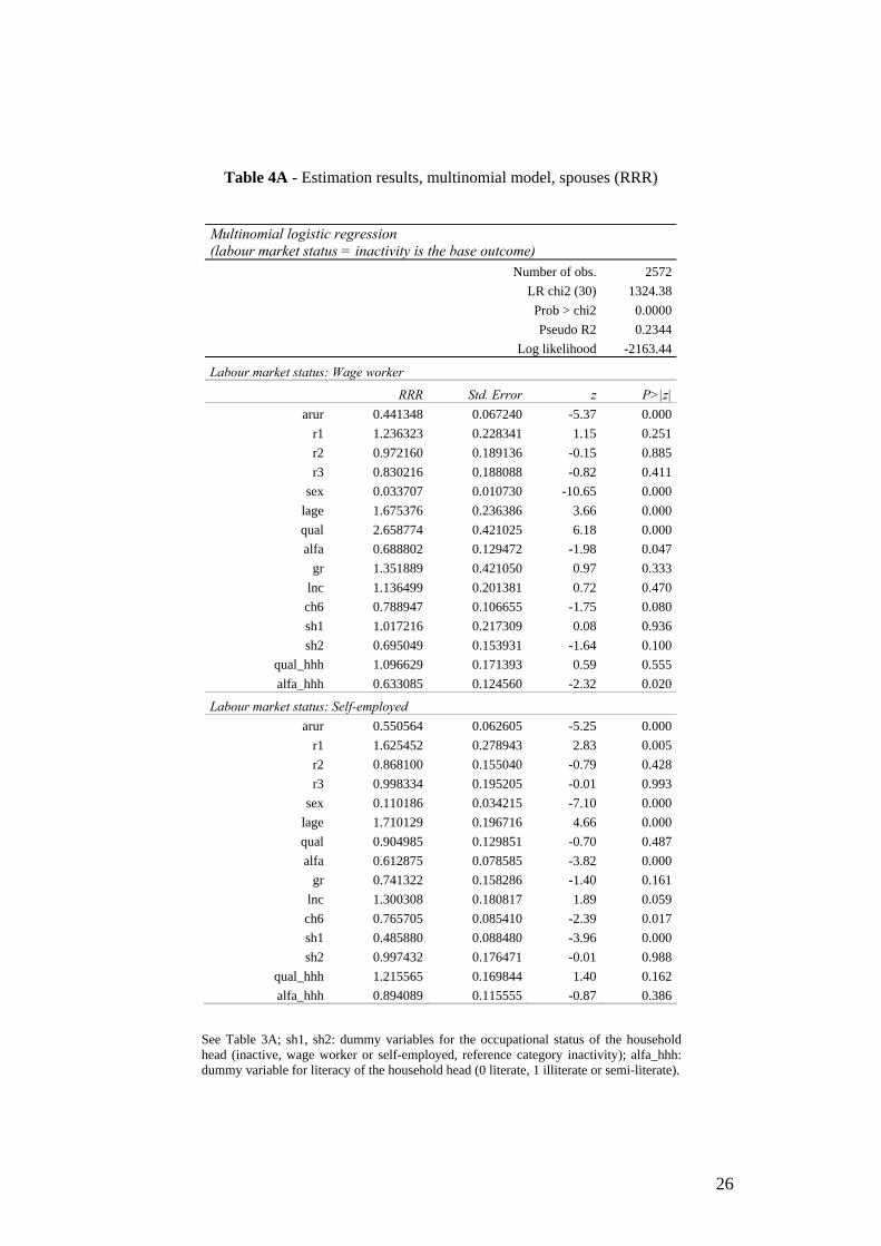
Table 4A - Estimation results, multinomial model, spouses (RRR)
Multinomial logistic regression (labour market status = inactivity is the base outcome)
Number of obs. 2572 LR chi2 (30) 1324.38 Prob > chi2 0.0000 Pseudo R2 0.2344
Log likelihood -2163.44
Labour market status: Wage worker RRR Std. Error z P>|z|
arur 0.441348 0.067240 -5.37 0.000 r1 1.236323 0.228341 1.15 0.251 r2 0.972160 0.189136 -0.15 0.885 r3 0.830216 0.188088 -0.82 0.411
sex 0.033707 0.010730 -10.65 0.000 lage 1.675376 0.236386 3.66 0.000 qual 2.658774 0.421025 6.18 0.000 alfa 0.688802 0.129472 -1.98 0.047
gr 1.351889 0.421050 0.97 0.333 lnc 1.136499 0.201381 0.72 0.470 ch6 0.788947 0.106655 -1.75 0.080 sh1 1.017216 0.217309 0.08 0.936 sh2 0.695049 0.153931 -1.64 0.100
qual_hhh 1.096629 0.171393 0.59 0.555 alfa_hhh 0.633085 0.124560 -2.32 0.020
Labour market status: Self-employed arur 0.550564 0.062605 -5.25 0.000
r1 1.625452 0.278943 2.83 0.005 r2 0.868100 0.155040 -0.79 0.428 r3 0.998334 0.195205 -0.01 0.993
sex 0.110186 0.034215 -7.10 0.000 lage 1.710129 0.196716 4.66 0.000 qual 0.904985 0.129851 -0.70 0.487 alfa 0.612875 0.078585 -3.82 0.000
gr 0.741322 0.158286 -1.40 0.161 lnc 1.300308 0.180817 1.89 0.059 ch6 0.765705 0.085410 -2.39 0.017 sh1 0.485880 0.088480 -3.96 0.000 sh2 0.997432 0.176471 -0.01 0.988
qual_hhh 1.215565 0.169844 1.40 0.162 alfa_hhh 0.894089 0.115555 -0.87 0.386
See Table 3A; sh1, sh2: dummy variables for the occupational status of the household head (inactive, wage worker or self-employed, reference category inactivity); alfa_hhh: dummy variable for literacy of the household head (0 literate, 1 illiterate or semi-literate).
26
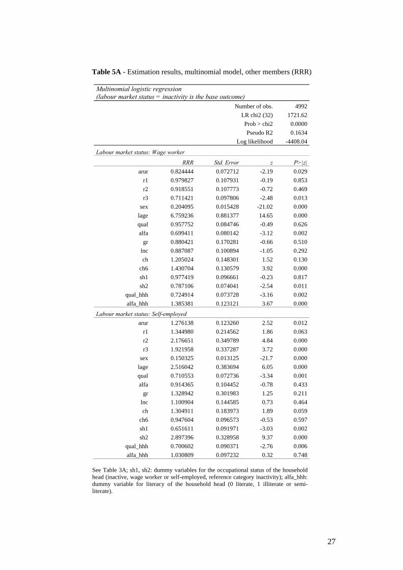
Table 5A - Estimation results, multinomial model, other members (RRR)
Multinomial logistic regression (labour market status = inactivity is the base outcome)
Number of obs. 4992 LR chi2 (32) 1721.62 Prob > chi2 0.0000 Pseudo R2 0.1634
Log likelihood -4408.04
Labour market status: Wage worker RRR Std. Error z P>|z|
arur 0.824444 0.072712 -2.19 0.029 r1 0.979827 0.107931 -0.19 0.853 r2 0.918551 0.107773 -0.72 0.469 r3 0.711421 0.097806 -2.48 0.013
sex 0.204095 0.015428 -21.02 0.000 lage 6.759236 0.881377 14.65 0.000 qual 0.957752 0.084746 -0.49 0.626 alfa 0.699411 0.080142 -3.12 0.002
gr 0.880421 0.170281 -0.66 0.510 lnc 0.887087 0.100894 -1.05 0.292 ch 1.205024 0.148301 1.52 0.130
ch6 1.430704 0.130579 3.92 0.000 sh1 0.977419 0.096661 -0.23 0.817 sh2 0.787106 0.074041 -2.54 0.011
qual_hhh 0.724914 0.073728 -3.16 0.002 alfa_hhh 1.385381 0.123121 3.67 0.000
Labour market status: Self-employed arur 1.276138 0.123260 2.52 0.012
r1 1.344980 0.214562 1.86 0.063 r2 2.176651 0.349789 4.84 0.000 r3 1.921958 0.337287 3.72 0.000
sex 0.150325 0.013125 -21.7 0.000 lage 2.516042 0.383694 6.05 0.000 qual 0.710553 0.072736 -3.34 0.001 alfa 0.914365 0.104452 -0.78 0.433
gr 1.328942 0.301983 1.25 0.211 lnc 1.100904 0.144585 0.73 0.464 ch 1.304911 0.183973 1.89 0.059
ch6 0.947604 0.096573 -0.53 0.597 sh1 0.651611 0.091971 -3.03 0.002 sh2 2.897396 0.328958 9.37 0.000
qual_hhh 0.700602 0.090371 -2.76 0.006 alfa_hhh 1.030809 0.097232 0.32 0.748
See Table 3A; sh1, sh2: dummy variables for the occupational status of the household head (inactive, wage worker or self-employed, reference category inactivity); alfa_hhh: dummy variable for literacy of the household head (0 literate, 1 illiterate or semi-literate).
27
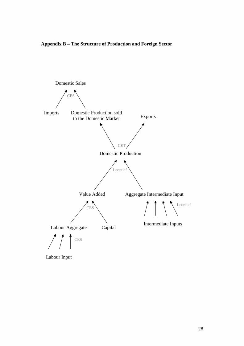
Appendix B – The Structure of Production and Foreign Sector Domestic Sales
Imports Domestic Production sold to the Domestic Market
Domestic Production
Exports
Aggregate Intermediate Input Value Added
Intermediate Inputs Capital Labour Aggregate
Labour Input
CES
CET
CES
CES
Leontief
Leontief
28
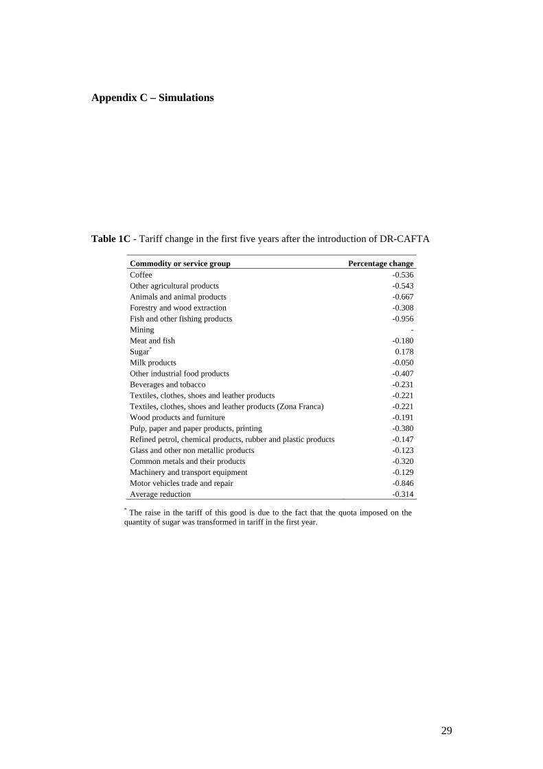
Appendix C – Simulations Table 1C - Tariff change in the first five years after the introduction of DR-CAFTA
Commodity or service group Percentage change Coffee -0.536 Other agricultural products -0.543 Animals and animal products -0.667 Forestry and wood extraction -0.308 Fish and other fishing products -0.956 Mining - Meat and fish -0.180 Sugar* 0.178 Milk products -0.050 Other industrial food products -0.407 Beverages and tobacco -0.231 Textiles, clothes, shoes and leather products -0.221 Textiles, clothes, shoes and leather products (Zona Franca) -0.221 Wood products and furniture -0.191 Pulp, paper and paper products, printing -0.380 Refined petrol, chemical products, rubber and plastic products -0.147 Glass and other non metallic products -0.123 Common metals and their products -0.320 Machinery and transport equipment -0.129 Motor vehicles trade and repair -0.846 Average reduction -0.314
* The raise in the tariff of this good is due to the fact that the quota imposed on the quantity of sugar was transformed in tariff in the first year.
29
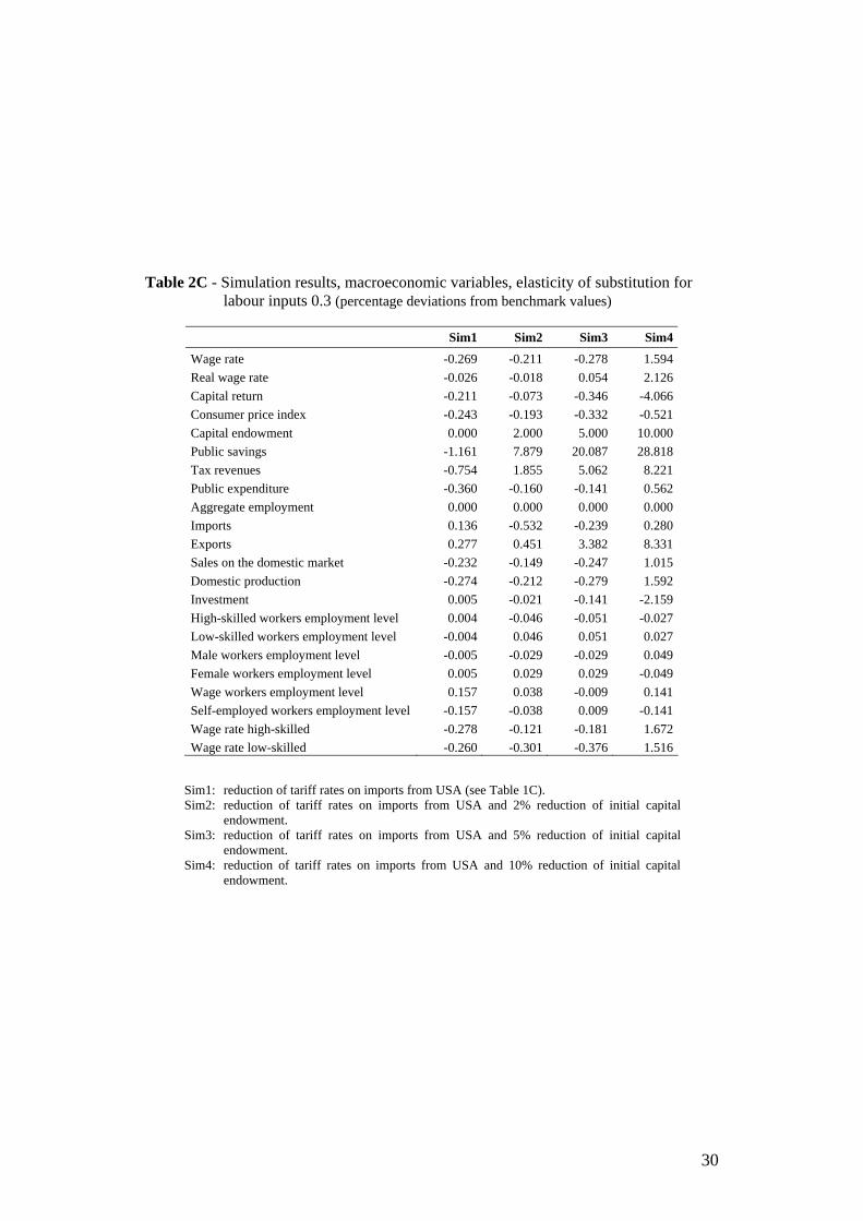
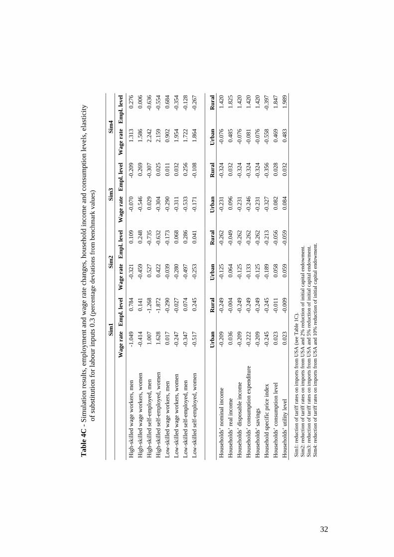
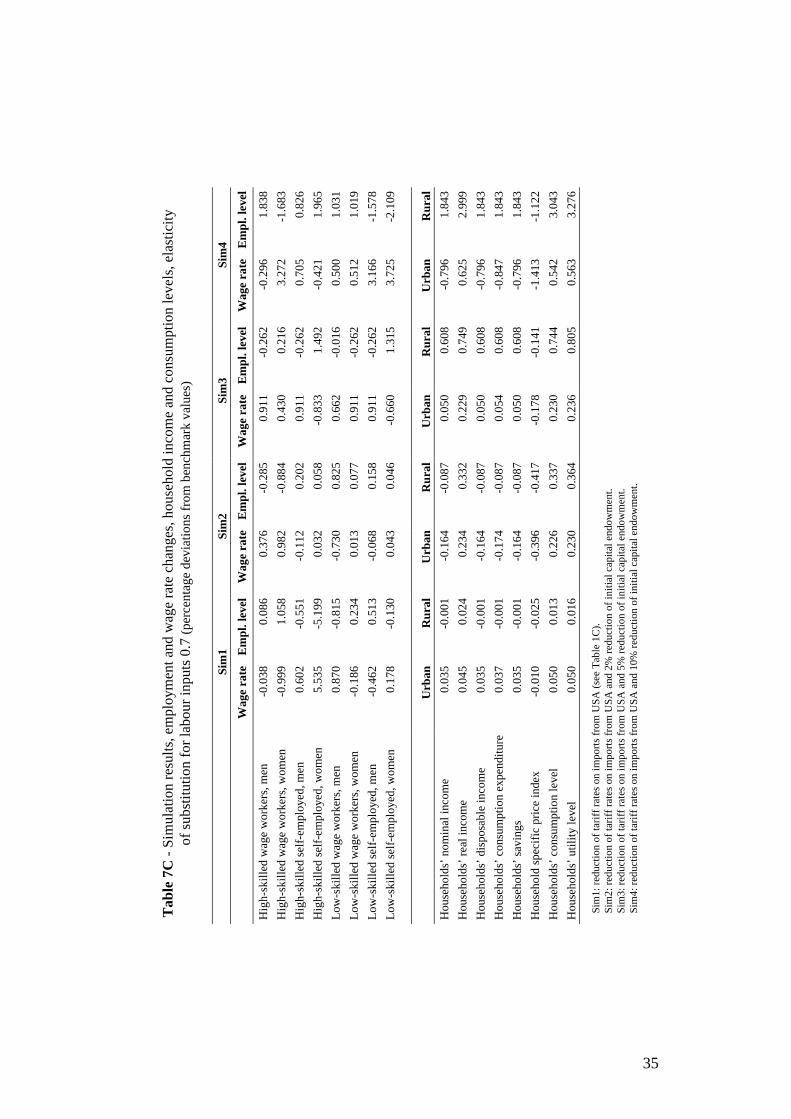
Table 2C - Simulation results, macroeconomic variables, elasticity of substitution for
labour inputs 0.3 (percentage deviations from benchmark values)
Sim1 Sim2 Sim3 Sim4
Wage rate -0.269 -0.211 -0.278 1.594 Real wage rate -0.026 -0.018 0.054 2.126 Capital return -0.211 -0.073 -0.346 -4.066 Consumer price index -0.243 -0.193 -0.332 -0.521 Capital endowment 0.000 2.000 5.000 10.000 Public savings -1.161 7.879 20.087 28.818 Tax revenues -0.754 1.855 5.062 8.221 Public expenditure -0.360 -0.160 -0.141 0.562 Aggregate employment 0.000 0.000 0.000 0.000 Imports 0.136 -0.532 -0.239 0.280 Exports 0.277 0.451 3.382 8.331 Sales on the domestic market -0.232 -0.149 -0.247 1.015 Domestic production -0.274 -0.212 -0.279 1.592 Investment 0.005 -0.021 -0.141 -2.159 High-skilled workers employment level 0.004 -0.046 -0.051 -0.027 Low-skilled workers employment level -0.004 0.046 0.051 0.027 Male workers employment level -0.005 -0.029 -0.029 0.049 Female workers employment level 0.005 0.029 0.029 -0.049 Wage workers employment level 0.157 0.038 -0.009 0.141 Self-employed workers employment level -0.157 -0.038 0.009 -0.141 Wage rate high-skilled -0.278 -0.121 -0.181 1.672 Wage rate low-skilled -0.260 -0.301 -0.376 1.516
Sim1: reduction of tariff rates on imports from USA (see Table 1C). Sim2: reduction of tariff rates on imports from USA and 2% reduction of initial capital
endowment. Sim3: reduction of tariff rates on imports from USA and 5% reduction of initial capital
endowment. Sim4: reduction of tariff rates on imports from USA and 10% reduction of initial capital
endowment.
30

Table 3C - Simulation results, sectoral changes (elasticity of substitution for labour
inputs 0.3) (percentage deviations from benchmark values)
Sim1 Sim2 Sim3 Sim4
Agricultural sectors Domestic production 2.774 -1.157 -3.697 -4.109 Sales on the domestic market 3.280 -1.180 -4.198 -5.128 Exports to USA 6.320 -0.876 -0.232 2.005 Exports to other countries -2.082 -1.702 0.297 2.648 Imports from USA -1.968 -0.145 1.574 2.623 Imports from other countries 7.438 -5.087 0.075 1.004
Industrial sectors Domestic production -3.504 -0.064 0.764 5.107 Sales on the domestic market -1.630 -0.017 0.514 3.046 Exports to USA -6.198 3.289 9.818 20.038 Exports to other countries -5.090 -0.250 2.592 7.932 Imports from USA 0.887 -2.833 -14.811 -17.900 Imports from other countries 0.110 0.064 3.235 4.643
Textile sectors Domestic production 0.986 -5.519 -11.585 -15.303 Sales on the domestic market 1.537 -4.381 -9.337 -14.614 Exports to USA 0.841 -8.619 -18.890 -21.642 Exports to other countries 0.649 -7.383 -15.803 -18.609 Imports from USA 1.996 -6.155 -14.148 -19.597 Imports from other countries 1.653 -6.498 -14.497 -19.936
Exporting sectors Domestic production 8.721 3.073 7.421 9.877 Sales on the domestic market 10.724 10.247 23.936 28.422 Exports to USA 5.380 4.846 12.002 16.662 Exports to other countries 7.682 0.077 0.569 2.397 Exports (all) 6.657 2.200 5.659 8.748 Imports from USA 2.133 -7.048 -16.243 -21.763 Imports from other countries 8.985 7.975 18.933 22.996 Imports (all) 8.276 6.421 15.294 18.366
· Agricultural sectors: coffee, sugar cane, corn, other agricultural products, animals and animal products, products of the forest and wood extraction, fishing.
· Industrial sectors: mining, energy, water, meat and fish, sugar, milk products, other food, beverages, tobacco, textiles (local and Zona Franca), wood products, paper, refined oil products, chemical and plastic products, glass, metal, machinery and equipment, construction.
· Textile sectors: textiles (local and Zona Franca). · Exporting sectors: all sectors with initial ratio exports/production grater than 50%
(coffee, tobacco, textiles – only Zona Franca, transport services).
31
Em
pl. l
evel
0.27
6 0.
006
-0.6
36
-0.5
54
0.68
4 -0
.354
-0
.128
-0
.267
Rur
al
1.42
0 1.
825
1.42
0 1.
420
1.42
0 -0
.397
1.
847
1.98
9
Sim
4
Wag
e ra
te
1.31
3 1.
586
2.24
2 2.
159
0.90
2 1.
954
1.72
2 1.
864
Urb
an
-0.0
76
0.48
5 -0
.076
-0
.081
-0
.076
-0
.558
0.
469
0.48
3
Em
pl. l
evel
-0.2
09
0.26
9 -0
.307
0.
025
0.01
1 0.
032
0.25
6 -0
.108
Rur
al
-0.3
24
0.03
2 -0
.324
-0
.324
-0
.324
-0
.356
0.
028
0.03
2
Sim
3
Wag
e ra
te
-0.0
70
-0.5
46
0.02
9 -0
.304
-0
.290
-0
.311
-0
.533
-0
.171
Urb
an
-0.2
31
0.09
6 -0
.231
-0
.246
-0
.231
-0
.327
0.
082
0.08
4
Em
pl. l
evel
0.10
9 0.
248
-0.7
35
-0.6
32
-0.1
73
0.06
8 0.
286
0.04
1
Rur
al
-0.2
62
-0.0
49
-0.2
62
-0.2
62
-0.2
62
-0.2
13
-0.0
56
-0.0
59
Sim
2
Wag
e ra
te
-0.3
21
-0.4
59
0.52
7 0.
422
-0.0
39
-0.2
80
-0.4
97
-0.2
53
Urb
an
-0.1
25
0.06
4 -0
.125
-0
.133
-0
.125
-0
.189
0.
058
0.05
9
Em
pl. l
evel
0.78
4 0.
141
-1.2
68
-1.8
72
-0.2
90
-0.0
27
0.07
4 0.
245
Rur
al
-0.2
49
-0.0
04
-0.2
49
-0.2
49
-0.2
49
-0.2
45
-0.0
11
-0.0
09
Sim
1
Wag
e ra
te
-1.0
49
-0.4
14
1.00
7 1.
628
0.01
7 -0
.247
-0
.347
-0
.517
Urb
an
-0.2
09
0.03
6 -0
.209
-0
.222
-0
.209
-0
.245
0.
023
0.02
3
Hig
h-sk
illed
wag
e w
orke
rs, m
en
Hig
h-sk
illed
wag
e w
orke
rs, w
omen
H
igh-
skill
ed se
lf-em
ploy
ed, m
en
Hig
h-sk
illed
self-
empl
oyed
, wom
en
Low
-ski
lled
wag
e w
orke
rs, m
en
Low
-ski
lled
wag
e w
orke
rs, w
omen
Lo
w-s
kille
d se
lf-em
ploy
ed, m
en
Low
-ski
lled
self-
empl
oyed
, wom
en
Hou
seho
lds’
nom
inal
inco
me
Hou
seho
lds’
real
inco
me
Hou
seho
lds’
dis
posa
ble
inco
me
Hou
seho
lds’
con
sum
ptio
n ex
pend
iture
H
ouse
hold
s’ sa
ving
s H
ouse
hold
spec
ific
pric
e in
dex
Hou
seho
lds’
con
sum
ptio
n le
vel
Hou
seho
lds’
util
ity le
vel
Tab
le 4
C -
Sim
ulat
ion
resu
lts, e
mpl
oym
ent a
nd w
age
rate
cha
nges
, hou
seho
ld in
com
e an
d co
nsum
ptio
n le
vels
, ela
stic
ity
of su
bstit
utio
n fo
r lab
our i
nput
s 0.3
(per
cent
age
devi
atio
ns fr
om b
ench
mar
k va
lues
)
Sim
1: re
duct
ion
of ta
riff r
ates
on
impo
rts fr
om U
SA (s
ee T
able
1C
). Si
m2:
redu
ctio
n of
tarif
f rat
es o
n im
ports
from
USA
and
2%
redu
ctio
n of
initi
al c
apita
l end
owm
ent.
Sim
3: re
duct
ion
of ta
riff r
ates
on
impo
rts fr
om U
SA a
nd 5
% re
duct
ion
of in
itial
cap
ital e
ndow
men
t. Si
m4:
redu
ctio
n of
tarif
f rat
es o
n im
ports
from
USA
and
10%
redu
ctio
n of
initi
al c
apita
l end
owm
ent.
32
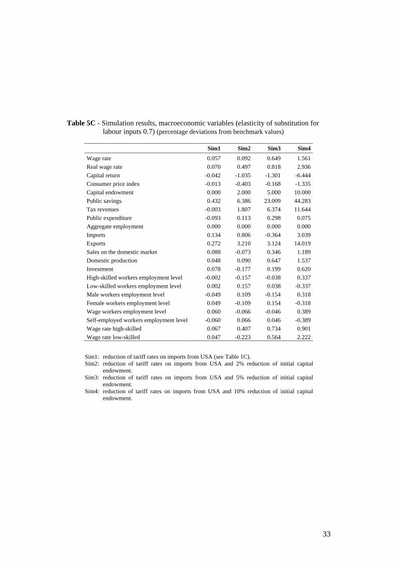
Table 5C - Simulation results, macroeconomic variables (elasticity of substitution for
labour inputs 0.7) (percentage deviations from benchmark values)
Sim1 Sim2 Sim3 Sim4
Wage rate 0.057 0.092 0.649 1.561 Real wage rate 0.070 0.497 0.818 2.936 Capital return -0.042 -1.035 -1.301 -6.444 Consumer price index -0.013 -0.403 -0.168 -1.335 Capital endowment 0.000 2.000 5.000 10.000 Public savings 0.432 6.386 23.009 44.283 Tax revenues -0.003 1.807 6.374 11.644 Public expenditure -0.093 0.113 0.298 0.075 Aggregate employment 0.000 0.000 0.000 0.000 Imports 0.134 0.806 -0.364 3.039 Exports 0.272 3.210 3.124 14.019 Sales on the domestic market 0.088 -0.073 0.346 1.189 Domestic production 0.048 0.090 0.647 1.537 Investment 0.078 -0.177 0.199 0.620 High-skilled workers employment level -0.002 -0.157 -0.038 0.337 Low-skilled workers employment level 0.002 0.157 0.038 -0.337 Male workers employment level -0.049 0.109 -0.154 0.318 Female workers employment level 0.049 -0.109 0.154 -0.318 Wage workers employment level 0.060 -0.066 -0.046 0.389 Self-employed workers employment level -0.060 0.066 0.046 -0.389 Wage rate high-skilled 0.067 0.407 0.734 0.901 Wage rate low-skilled 0.047 -0.223 0.564 2.222
Sim1: reduction of tariff rates on imports from USA (see Table 1C). Sim2: reduction of tariff rates on imports from USA and 2% reduction of initial capital
endowment. Sim3: reduction of tariff rates on imports from USA and 5% reduction of initial capital
endowment. Sim4: reduction of tariff rates on imports from USA and 10% reduction of initial capital
endowment.
33
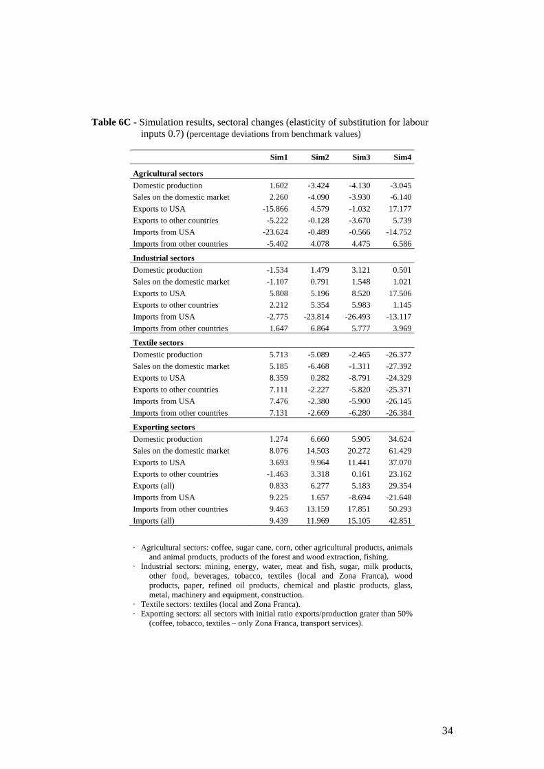
Table 6C - Simulation results, sectoral changes (elasticity of substitution for labour
inputs 0.7) (percentage deviations from benchmark values)
Sim1 Sim2 Sim3 Sim4
Agricultural sectors Domestic production 1.602 -3.424 -4.130 -3.045 Sales on the domestic market 2.260 -4.090 -3.930 -6.140 Exports to USA -15.866 4.579 -1.032 17.177 Exports to other countries -5.222 -0.128 -3.670 5.739 Imports from USA -23.624 -0.489 -0.566 -14.752 Imports from other countries -5.402 4.078 4.475 6.586
Industrial sectors Domestic production -1.534 1.479 3.121 0.501 Sales on the domestic market -1.107 0.791 1.548 1.021 Exports to USA 5.808 5.196 8.520 17.506 Exports to other countries 2.212 5.354 5.983 1.145 Imports from USA -2.775 -23.814 -26.493 -13.117 Imports from other countries 1.647 6.864 5.777 3.969
Textile sectors Domestic production 5.713 -5.089 -2.465 -26.377 Sales on the domestic market 5.185 -6.468 -1.311 -27.392 Exports to USA 8.359 0.282 -8.791 -24.329 Exports to other countries 7.111 -2.227 -5.820 -25.371 Imports from USA 7.476 -2.380 -5.900 -26.145 Imports from other countries 7.131 -2.669 -6.280 -26.384
Exporting sectors Domestic production 1.274 6.660 5.905 34.624 Sales on the domestic market 8.076 14.503 20.272 61.429 Exports to USA 3.693 9.964 11.441 37.070 Exports to other countries -1.463 3.318 0.161 23.162 Exports (all) 0.833 6.277 5.183 29.354 Imports from USA 9.225 1.657 -8.694 -21.648 Imports from other countries 9.463 13.159 17.851 50.293 Imports (all) 9.439 11.969 15.105 42.851
· Agricultural sectors: coffee, sugar cane, corn, other agricultural products, animals and animal products, products of the forest and wood extraction, fishing.
· Industrial sectors: mining, energy, water, meat and fish, sugar, milk products, other food, beverages, tobacco, textiles (local and Zona Franca), wood products, paper, refined oil products, chemical and plastic products, glass, metal, machinery and equipment, construction.
· Textile sectors: textiles (local and Zona Franca). · Exporting sectors: all sectors with initial ratio exports/production grater than 50%
(coffee, tobacco, textiles – only Zona Franca, transport services).
34
Em
pl. l
evel
1.83
8 -1
.683
0.
826
1.96
5 1.
031
1.01
9 -1
.578
-2
.109
Rur
al
1.84
3 2.
999
1.84
3 1.
843
1.84
3 -1
.122
3.
043
3.27
6
Sim
4
Wag
e ra
te
-0.2
96
3.27
2 0.
705
-0.4
21
0.50
0 0.
512
3.16
6 3.
725
Urb
an
-0.7
96
0.62
5 -0
.796
-0
.847
-0
.796
-1
.413
0.
542
0.56
3
Em
pl. l
evel
-0.2
62
0.21
6 -0
.262
1.
492
-0.0
16
-0.2
62
-0.2
62
1.31
5
Rur
al
0.60
8 0.
749
0.60
8 0.
608
0.60
8 -0
.141
0.
744
0.80
5
Sim
3
Wag
e ra
te
0.91
1 0.
430
0.91
1 -0
.833
0.
662
0.91
1 0.
911
-0.6
60
Urb
an
0.05
0 0.
229
0.05
0 0.
054
0.05
0 -0
.178
0.
230
0.23
6
Em
pl. l
evel
-0.2
85
-0.8
84
0.20
2 0.
058
0.82
5 0.
077
0.15
8 0.
046
Rur
al
-0.0
87
0.33
2 -0
.087
-0
.087
-0
.087
-0
.417
0.
337
0.36
4
Sim
2
Wag
e ra
te
0.37
6 0.
982
-0.1
12
0.03
2 -0
.730
0.
013
-0.0
68
0.04
3
Urb
an
-0.1
64
0.23
4 -0
.164
-0
.174
-0
.164
-0
.396
0.
226
0.23
0
Em
pl. l
evel
0.08
6 1.
058
-0.5
51
-5.1
99
-0.8
15
0.23
4 0.
513
-0.1
30
Rur
al
-0.0
01
0.02
4 -0
.001
-0
.001
-0
.001
-0
.025
0.
013
0.01
6
Sim
1
Wag
e ra
te
-0.0
38
-0.9
99
0.60
2 5.
535
0.87
0 -0
.186
-0
.462
0.
178
Urb
an
0.03
5 0.
045
0.03
5 0.
037
0.03
5 -0
.010
0.
050
0.05
0
Hig
h-sk
illed
wag
e w
orke
rs, m
en
Hig
h-sk
illed
wag
e w
orke
rs, w
omen
H
igh-
skill
ed se
lf-em
ploy
ed, m
en
Hig
h-sk
illed
self-
empl
oyed
, wom
en
Low
-ski
lled
wag
e w
orke
rs, m
en
Low
-ski
lled
wag
e w
orke
rs, w
omen
Lo
w-s
kille
d se
lf-em
ploy
ed, m
en
Low
-ski
lled
self-
empl
oyed
, wom
en
Hou
seho
lds’
nom
inal
inco
me
Hou
seho
lds’
real
inco
me
Hou
seho
lds’
dis
posa
ble
inco
me
Hou
seho
lds’
con
sum
ptio
n ex
pend
iture
H
ouse
hold
s’ sa
ving
s H
ouse
hold
spec
ific
pric
e in
dex
Hou
seho
lds’
con
sum
ptio
n le
vel
Hou
seho
lds’
util
ity le
vel
Tab
le 7
C -
Sim
ulat
ion
resu
lts, e
mpl
oym
ent a
nd w
age
rate
cha
nges
, hou
seho
ld in
com
e an
d co
nsum
ptio
n le
vels
, ela
stic
ity
of su
bstit
utio
n fo
r lab
our i
nput
s 0.7
(per
cent
age
devi
atio
ns fr
om b
ench
mar
k va
lues
)
Sim
1: re
duct
ion
of ta
riff r
ates
on
impo
rts fr
om U
SA (s
ee T
able
1C
). Si
m2:
redu
ctio
n of
tarif
f rat
es o
n im
ports
from
USA
and
2%
redu
ctio
n of
initi
al c
apita
l end
owm
ent.
Sim
3: re
duct
ion
of ta
riff r
ates
on
impo
rts fr
om U
SA a
nd 5
% re
duct
ion
of in
itial
cap
ital e
ndow
men
t. Si
m4:
redu
ctio
n of
tarif
f rat
es o
n im
ports
from
USA
and
10%
redu
ctio
n of
initi
al c
apita
l end
owm
ent.
35
Table 8C - Simulation results, macroeconomic variables, elasticity of substitution for
labour inputs equal to value added aggregation sectoral elasticities (percentage deviations from benchmark values)
Sim1 Sim2 Sim3 Sim4
Wage rate 0.197 0.172 0.399 0.813 Real wage rate 0.173 0.483 0.406 1.236 Capital return -0.082 -0.900 -0.386 -2.106 Consumer price index 0.024 -0.309 -0.007 -0.417 Capital endowment 0.000 2.000 5.000 10.000 Public savings 0.759 9.952 23.589 30.675 Tax revenues 0.305 2.748 6.666 8.967 Public expenditure 0.085 0.122 0.410 0.771 Aggregate employment 0.000 0.000 0.000 0.000 Imports 0.288 1.313 0.728 0.068 Exports 0.591 4.254 5.376 7.894 Sales on the domestic market 0.223 0.047 0.357 0.597 Domestic production 0.188 0.169 0.390 0.797 Investment 0.081 0.277 0.157 -1.990 High-skilled workers employment level -0.027 -0.146 -0.148 -0.354 Low-skilled workers employment level 0.027 0.146 0.148 0.354 Male workers employment level -0.021 -0.115 -0.128 0.143 Female workers employment level 0.021 0.115 0.128 -0.143 Wage workers employment level -0.072 -0.127 -0.179 -0.375 Self-employed workers employment level 0.072 0.127 0.179 0.375 Wage rate high-skilled 0.254 0.468 0.706 1.532 Wage rate low-skilled 0.139 -0.123 0.092 0.094
Sim1: reduction of tariff rates on imports from USA (see Table 1C). Sim2: reduction of tariff rates on imports from USA and 2% reduction of initial capital
endowment. Sim3: reduction of tariff rates on imports from USA and 5% reduction of initial capital
endowment. Sim4: reduction of tariff rates on imports from USA and 10% reduction of initial capital
endowment.
36
Table 9C - Simulation results, sectoral changes (elasticity of substitution for labour
inputs equal to value added aggregation sectoral elasticities) (percentage deviations from benchmark values)
Sim1 Sim2 Sim3 Sim4
Agricultural sectors Domestic production 3.613 -6.414 -6.367 -7.150 Sales on the domestic market 4.681 -5.978 -0.927 -1.100 Exports to USA -20.053 -8.085 -37.486 -42.262 Exports to other countries -7.365 -4.892 -22.812 -24.609 Imports from USA -33.527 1.091 2.940 4.747 Imports from other countries -4.675 -0.614 -1.355 -0.622
Industrial sectors Domestic production -1.623 2.460 3.030 5.484 Sales on the domestic market -1.162 1.266 0.704 1.923 Exports to USA 8.536 10.957 26.881 36.899 Exports to other countries 3.041 8.609 15.385 19.393 Imports from USA -2.395 -25.514 -34.416 -40.961 Imports from other countries 2.085 8.054 9.342 9.996
Textile sectors Domestic production 9.145 1.516 -1.092 -10.006 Sales on the domestic market 7.794 1.394 -1.261 -8.856 Exports to USA 13.848 2.192 -1.298 -17.184 Exports to other countries 11.799 1.777 -1.104 -13.775 Imports from USA 11.399 2.155 -1.262 -14.233 Imports from other countries 11.054 1.812 -1.606 -14.595
Exporting sectors Domestic production 2.149 5.895 6.392 9.272 Sales on the domestic market 11.256 17.710 37.849 52.240 Exports to USA 5.917 10.246 16.334 22.094 Exports to other countries -1.497 1.024 -6.356 -8.347 Exports (all) 1.804 5.130 3.746 5.206 Imports from USA 14.188 3.553 0.937 -15.084 Imports from other countries 13.587 16.982 36.799 47.538 Imports (all) 13.649 15.593 33.090 41.060
· Agricultural sectors: coffee, sugar cane, corn, other agricultural products, animals and animal products, products of the forest and wood extraction, fishing.
· Industrial sectors: mining, energy, water, meat and fish, sugar, milk products, other food, beverages, tobacco, textiles (local and Zona Franca), wood products, paper, refined oil products, chemical and plastic products, glass, metal, machinery and equipment, construction.
· Textile sectors: textiles (local and Zona Franca). · Exporting sectors: all sectors with initial ratio exports/production grater than 50%
(coffee, tobacco, textiles – only Zona Franca, transport services).
37
Em
pl. l
evel
-1.3
94
-0.3
16
0.16
5 -0
.703
-0
.199
0.
294
2.11
1 -1
.211
Rur
al
0.16
8 0.
619
0.16
8 0.
168
0.16
8 -0
.448
0.
639
0.68
3
Sim
4
Wag
e ra
te
2.22
3 1.
117
0.63
2 1.
510
0.99
8 0.
502
-1.2
87
2.03
3
Urb
an
0.08
7 0.
490
0.08
7 0.
093
0.08
7 -0
.401
0.
501
0.51
3
Em
pl. l
evel
-1.3
56
1.06
5 0.
196
-0.2
31
-0.3
60
0.83
9 0.
938
-0.5
99
Rur
al
0.13
5 0.
167
0.13
5 0.
135
0.13
5 -0
.033
0.
161
0.17
3
Sim
3
Wag
e ra
te
1.77
0 -0
.668
0.
194
0.62
2 0.
753
-0.4
45
-0.5
43
0.99
6
Urb
an
0.19
2 0.
191
0.19
2 0.
204
0.19
2 0.
001
0.20
7 0.
211
Em
pl. l
evel
-0.8
07
0.64
1 -0
.427
0.
457
-0.3
47
0.42
9 0.
775
0.01
0
Rur
al
-0.0
47
0.27
7 -0
.047
-0
.047
-0
.047
-0
.324
0.
278
0.29
9
Sim
2
Wag
e ra
te
0.98
3 -0
.469
0.
598
-0.2
88
0.51
7 -0
.260
-0
.602
0.
159
Urb
an
-0.0
75
0.23
4 -0
.075
-0
.079
-0
.075
-0
.308
0.
229
0.23
6
Em
pl. l
evel
0.13
6 0.
518
-0.3
49
-4.6
67
-1.4
16
0.47
8 0.
843
0.14
8
Rur
al
0.07
4 0.
076
0.07
4 0.
074
0.07
4 -0
.002
0.
065
0.07
1
Sim
1
Wag
e ra
te
0.05
2 -0
.328
0.
538
5.09
3 1.
627
-0.2
89
-0.6
50
0.03
9
Urb
an
0.12
0 0.
087
0.12
0 0.
127
0.12
0 0.
033
0.10
0 0.
100
Hig
h-sk
illed
wag
e w
orke
rs. m
en
Hig
h-sk
illed
wag
e w
orke
rs. w
omen
H
igh-
skill
ed se
lf-em
ploy
ed. m
en
Hig
h-sk
illed
self-
empl
oyed
. wom
en
Low
-ski
lled
wag
e w
orke
rs. m
en
Low
-ski
lled
wag
e w
orke
rs. w
omen
Lo
w-s
kille
d se
lf-em
ploy
ed. m
en
Low
-ski
lled
self-
empl
oyed
. wom
en
Hou
seho
lds’
nom
inal
inco
me
Hou
seho
lds’
real
inco
me
Hou
seho
lds’
dis
posa
ble
inco
me
Hou
seho
lds’
con
sum
ptio
n ex
pend
iture
H
ouse
hold
s’ sa
ving
s H
ouse
hold
spec
ific
pric
e in
dex
Hou
seho
lds’
con
sum
ptio
n le
vel
Hou
seho
lds’
util
ity le
vel
Tab
le 1
0C -
Sim
ulat
ion
resu
lts, e
mpl
oym
ent a
nd w
age
rate
cha
nges
, hou
seho
ld in
com
e an
d co
nsum
ptio
n le
vels
, ela
stic
ity
of su
bstit
utio
n fo
r lab
our i
nput
s equ
al to
val
ue a
dded
agg
rega
tion
sect
oral
ela
stic
ities
(per
cent
age
devi
atio
ns
from
ben
chm
ark
valu
es)
Sim
1: re
duct
ion
of ta
riff r
ates
on
impo
rts fr
om U
SA (s
ee T
able
1C
). Si
m2:
redu
ctio
n of
tarif
f rat
es o
n im
ports
from
USA
and
2%
redu
ctio
n of
initi
al c
apita
l end
owm
ent.
Sim
3: re
duct
ion
of ta
riff r
ates
on
impo
rts fr
om U
SA a
nd 5
% re
duct
ion
of in
itial
cap
ital e
ndow
men
t. Si
m4:
redu
ctio
n of
tarif
f rat
es o
n im
ports
from
USA
and
10%
redu
ctio
n of
initi
al c
apita
l end
owm
ent.
38
0.04
%
0.09
%
-1.1
5%
-1.4
9%
-1.4
4%
-1.6
1%
-1.5
3%
-1.5
6%
Rur
al
1.86
%
0.25
%
-0.4
9%
-0.8
1%
Sim
4
Urb
an
2.09
%
-0.1
7%
-2.0
6%
-2.8
5%
-0.0
9%
-0.1
7%
0.12
%
-0.1
4%
-0.0
9%
-0.2
6%
-0.2
0%
-0.4
4%
Rur
al
1.72
%
-0.0
9%
0.14
%
0.10
%
Sim
3
Urb
an
2.02
%
-0.2
7%
0.10
%
-0.6
1%
-0.1
2%
-0.1
7%
-0.0
4%
-0.2
7%
-0.3
4%
-0.4
8%
-0.4
5%
-0.7
0%
Rur
al
1.75
%
-0.0
8%
0.07
%
0.10
%
Sim
2
Urb
an
1.96
%
-0.2
9%
-0.2
0%
-1.0
2%
0.12
%
0.27
%
-0.0
8%
0.14
%
-0.0
6%
-0.2
1%
-0.1
5%
-0.3
9%
Rur
al
1.68
%
-0.1
8%
0.00
%
0.10
%
Sim
1
Urb
an
2.31
%
0.22
%
-0.2
0%
0.20
%
60.6
6 79
.60
58.1
8 35
.35
32.3
4 18
.23
22.6
2 12
.78
Rur
al
55.3
2 58
.72
77.0
0 53
.83
Ben
chm
ark
Urb
an
57.6
6 72
.25
43.4
5 20
.89
Gen
eral
Ex
trem
e G
ener
al
Extre
me
Gen
eral
Ex
trem
e
Gen
eral
Ex
trem
e
Gin
i ind
ex
Thei
l ind
ex
P 0 P 1 P 2
Gin
i ind
ex
Thei
l ind
ex
P 0 Tab
le 1
1C -
Mic
roec
onom
ic re
sults
, inc
ome
dist
ribut
ion
and
pove
rty c
hang
es (e
last
icity
of s
ubst
itutio
n fo
r lab
our i
nput
s 0.3
)
Sim
1: re
duct
ion
of ta
riff r
ates
on
impo
rts fr
om U
SA (s
ee T
able
1C
). Si
m2:
redu
ctio
n of
tarif
f rat
es o
n im
ports
from
USA
and
2%
redu
ctio
n of
initi
al c
apita
l end
owm
ent.
Sim
3: re
duct
ion
of ta
riff r
ates
on
impo
rts fr
om U
SA a
nd 5
% re
duct
ion
of in
itial
cap
ital e
ndow
men
t. Si
m4:
redu
ctio
n of
tarif
f rat
es o
n im
ports
from
USA
and
10%
redu
ctio
n of
initi
al c
apita
l end
owm
ent.
All
the
indi
ces a
re c
ompu
ted
on p
er-c
apita
gro
ss in
com
e.
The
pove
rty li
ne fo
r the
gen
eral
pov
erty
rate
is fi
xed
at a
leve
l of 5
157
$C p
er y
ear,
whi
le th
e ex
trem
e po
verty
line
is 2
691
$C.
P0 is
the
“hea
dcou
nt ra
tio”:
it m
easu
res t
he in
cide
nce
of p
over
ty a
s the
pro
porti
on o
f tot
al p
opul
atio
n ly
ing
belo
w th
e po
verty
line
. P1
is th
e “p
over
ty g
ap ra
tio”,
whi
ch m
easu
res t
he in
tens
ity o
f pov
erty
. as i
t ref
lect
s how
far t
he p
oor a
re fr
om th
e po
verty
line
. P2
is a
lso
calle
d “s
ever
ity o
f pov
erty
inde
x” a
s it g
ives
an
indi
catio
n of
the
degr
ee o
f ine
qual
ity a
mon
g th
e po
or.
39
-0.1
8%
-0.7
8%
-1.4
0%
-2.3
6%
-2.0
7%
-2.1
5%
-2.1
2%
-1.8
8%
Rur
al
1.73
%
-0.0
3%
-0.2
1%
-1.4
1%
Sim
4
Urb
an
1.71
%
-1.4
2%
-3.0
4%
-4.2
8%
-0.1
1%
-0.3
0%
-0.2
9%
-0.6
1%
-0.6
7%
-1.1
1%
-0.9
0%
-1.3
8%
Rur
al
1.59
%
-0.3
1%
-0.0
7%
-0.6
1%
Sim
3
Urb
an
2.07
%
-0.3
3%
-0.5
9%
-0.6
1%
-0.0
4%
-0.0
7%
0.04
%
-0.3
4%
-0.2
6%
-0.3
1%
-0.3
0%
-0.2
6%
Rur
al
1.80
%
0.13
%
0.14
%
0.30
%
Sim
2
Urb
an
-1.6
3%
-0.3
0%
-0.1
0%
-1.6
3%
0.02
%
0.00
%
-0.6
6%
-1.0
8%
-1.1
1%
-1.0
0%
-1.0
5%
-0.7
3%
Rur
al
1.74
%
-0.0
7%
-0.2
8%
-0.4
0%
Sim
1
Urb
an
1.91
%
-0.5
7%
-1.9
6%
-2.4
4%
60.6
6 79
.60
58.1
8 35
.35
32.3
4 18
.23
22.6
2 12
.78
Rur
al
55.3
2 58
.72
77.0
0 53
.83
Ben
chm
ark
Urb
an
57.6
6 72
.25
43.4
5 20
.89
Gen
eral
Ex
trem
e G
ener
al
Extre
me
Gen
eral
Ex
trem
e
Gen
eral
Ex
trem
e
Gin
i ind
ex
Thei
l ind
ex
P 0 P 1 P 2
Gin
i ind
ex
Thei
l ind
ex
P 0 Tab
le 1
2C -
Mic
roec
onom
ic re
sults
, inc
ome
dist
ribut
ion
and
pove
rty c
hang
es (e
last
icity
of s
ubst
itutio
n fo
r lab
our i
nput
s 0.7
)
Sim
1: re
duct
ion
of ta
riff r
ates
on
impo
rts fr
om U
SA (s
ee T
able
1C
). Si
m2:
redu
ctio
n of
tarif
f rat
es o
n im
ports
from
USA
and
2%
redu
ctio
n of
initi
al c
apita
l end
owm
ent.
Sim
3: re
duct
ion
of ta
riff r
ates
on
impo
rts fr
om U
SA a
nd 5
% re
duct
ion
of in
itial
cap
ital e
ndow
men
t. Si
m4:
redu
ctio
n of
tarif
f rat
es o
n im
ports
from
USA
and
10%
redu
ctio
n of
initi
al c
apita
l end
owm
ent.
All
the
indi
ces a
re c
ompu
ted
on p
er-c
apita
gro
ss in
com
e.
The
pove
rty li
ne fo
r the
gen
eral
pov
erty
rate
is fi
xed
at a
leve
l of 5
157
$C p
er y
ear,
whi
le th
e ex
trem
e po
verty
line
is 2
691
$C.
P0 is
the
“hea
dcou
nt ra
tio”:
it m
easu
res t
he in
cide
nce
of p
over
ty a
s the
pro
porti
on o
f tot
al p
opul
atio
n ly
ing
belo
w th
e po
verty
line
. P1
is th
e “p
over
ty g
ap ra
tio”,
whi
ch m
easu
res t
he in
tens
ity o
f pov
erty
. as i
t ref
lect
s how
far t
he p
oor a
re fr
om th
e po
verty
line
. P2
is a
lso
calle
d “s
ever
ity o
f pov
erty
inde
x” a
s it g
ives
an
indi
catio
n of
the
degr
ee o
f ine
qual
ity a
mon
g th
e po
or.
40
-0.1
4%
-0.2
6%
-0.7
8%
-1.0
8%
-1.2
0%
-1.3
2%
-1.2
8%
-1.2
7%
Rur
al
0.04
%
0.00
%
-0.1
4%
0.00
%
Sim
4
Urb
an
-0.4
1%
-0.6
8%
-1.6
7%
-3.2
6%
-0.1
4%
-0.3
0%
-0.4
1%
-0.8
1%
-0.8
1%
-0.7
5%
-0.8
5%
-0.6
2%
Rur
al
0.05
%
0.10
%
0.07
%
0.00
%
Sim
3
Urb
an
-0.3
7%
-0.6
5%
-1.0
8%
-2.4
4%
-0.1
4%
-0.3
1%
-0.3
3%
-0.7
4%
-0.5
8%
-0.5
6%
-0.6
2%
-0.5
0%
Rur
al
0.01
%
0.02
%
0.14
%
0.00
%
Sim
2
Urb
an
-0.3
5%
-0.6
2%
-0.9
8%
-2.2
4%
0.05
%
0.14
%
-0.4
5%
-0.4
7%
-0.5
6%
-0.3
5%
-0.4
9%
-0.3
6%
Rur
al
0.17
%
0.21
%
0.00
%
0.00
%
Sim
1
Urb
an
-0.1
2%
-0.1
6%
-1.0
8%
-1.4
3%
60.6
6 79
.60
58.1
8 35
.35
32.3
4 18
.23
22.6
2 12
.78
Rur
al
55.3
2 58
.72
77.0
0 53
.83
Ben
chm
ark
Urb
an
57.6
6 72
.25
43.4
5 20
.89
Gen
eral
Ex
trem
e G
ener
al
Extre
me
Gen
eral
Ex
trem
e
Gen
eral
Ex
trem
e
Gin
i ind
ex
Thei
l ind
ex
P 0 P 1 P 2
Gin
i ind
ex
Thei
l ind
ex
P 0 Tab
le 1
3C -
Mic
roec
onom
ic re
sults
, inc
ome
dist
ribut
ion
and
pove
rty c
hang
es (e
last
icity
of s
ubst
itutio
n fo
r lab
our i
nput
s equ
al to
val
ue a
dded
agg
rega
tion
sect
oral
ela
stic
ities
)
Sim
1: re
duct
ion
of ta
riff r
ates
on
impo
rts fr
om U
SA (s
ee T
able
1C
). Si
m2:
redu
ctio
n of
tarif
f rat
es o
n im
ports
from
USA
and
2%
redu
ctio
n of
initi
al c
apita
l end
owm
ent.
Sim
3: re
duct
ion
of ta
riff r
ates
on
impo
rts fr
om U
SA a
nd 5
% re
duct
ion
of in
itial
cap
ital e
ndow
men
t. Si
m4:
redu
ctio
n of
tarif
f rat
es o
n im
ports
from
USA
and
10%
redu
ctio
n of
initi
al c
apita
l end
owm
ent.
All
the
indi
ces a
re c
ompu
ted
on p
er-c
apita
gro
ss in
com
e.
The
pove
rty li
ne fo
r the
gen
eral
pov
erty
rate
is fi
xed
at a
leve
l of 5
157
$C p
er y
ear,
whi
le th
e ex
trem
e po
verty
line
is 2
691
$C.
P0 is
the
“hea
dcou
nt ra
tio”:
it m
easu
res t
he in
cide
nce
of p
over
ty a
s the
pro
porti
on o
f tot
al p
opul
atio
n ly
ing
belo
w th
e po
verty
line
. P1
is th
e “p
over
ty g
ap ra
tio”,
whi
ch m
easu
res t
he in
tens
ity o
f pov
erty
. as i
t ref
lect
s how
far t
he p
oor a
re fr
om th
e po
verty
line
. P2
is a
lso
calle
d “s
ever
ity o
f pov
erty
inde
x” a
s it g
ives
an
indi
catio
n of
the
degr
ee o
f ine
qual
ity a
mon
g th
e po
or.
41
Recommended