The Pareto Frontier forRandom Mechanisms∗
Timo Mennle
University of Zurich
Sven Seuken
University of Zurich
First version: February 13, 2015
This version: January 10, 2017
Abstract
We study the trade-offs between strategyproofness and other desiderata, such asefficiency or fairness, that often arise in the design of random ordinal mechanisms.We use ε-approximate strategyproofness to define manipulability, a measure toquantify the incentive properties of non-strategyproof mechanisms, and we in-troduce the deficit, a measure to quantify the performance of mechanisms withrespect to another desideratum. When this desideratum is incompatible withstrategyproofness, mechanisms that trade off manipulability and deficit optimallyform the Pareto frontier. Our main contribution is a structural characterizationof this Pareto frontier, and we present algorithms that exploit this structure tocompute it. To illustrate its shape, we apply our results for two different desiderata,namely Plurality and Veto scoring, in settings with 3 alternatives and up to 18agents.
Keywords: Random Mechanisms, Pareto Frontier, Ordinal Mechanisms, Strategyproof-ness, Approximate Strategyproofness, Positional Scoring, Linear Programming
JEL: D71, D82
∗ Department of Informatics, University of Zurich, Switzerland, Email: {mennle, seuken}@ifi.uzh.ch. Updates avail-able from https://www.ifi.uzh.ch/ce/publications/EFF.pdf. We would like to thank (in alphabetical order) DanielAbaecherli, Haris Aziz, Gianluca Brero, Albin Erlanson, Bettina Klaus, Christian Kroer, Dmitry Moor, Ariel Pro-caccia, Tuomas Sandholm, Arunava Sen, Steffen Schuldenzucker, William Thomson, and Utku Unver for helpfulcomments on this work. Furthermore, we are thankful for the feedback we received from participants at COST COM-SOC Meeting 2016 (Istanbul, Turkey) and multiple anonymous referees at EC’15 and EC’16. Any errors remain ourown. A 1-page abstract based on this paper has been published in the conference proceedings of EC’16 (Mennle andSeuken, 2016). Part of this research was supported by the SNSF (Swiss National Science Foundation) under grant#156836.
1
1. Introduction
In many situations, a group of individuals has to make a collective decision by selecting
an alternative: who should be the next president? who gets a seat at which public school?
or where to build a new stadium? Mechanisms are systematic procedures to make such
decisions. Formally, a mechanism collects the individuals’ (or agents’ ) preferences and
selects an alternative based on this input. While the goal is to select an alternative that
is desirable for society as a whole, it may be possible for individual agents to manipulate
the outcome to their own advantage by being insincere about their preferences. However,
if these agents are lying about their preferences, the mechanism will have difficulty in
determining an outcome that is desirable with respect to the true preferences. Therefore,
incentives for truthtelling are a major concern in mechanism design. In this paper, we
consider ordinal mechanisms with random outcomes. Such mechanisms collect preference
orders and select lotteries over alternatives. We formulate our results for the full domain
where agents can have any weak or strict preferences, but our results continue to hold
on many domain restrictions, including the domain of strict preferences, the assignment
domain, and the two-sided matching domain.
1.1. The Curse of Strategyproofness
Strategyproof mechanisms make truthful reporting a dominant strategy for all agents and
it is therefore the “gold standard” among the incentive concepts. However, the seminal
impossibility results by Gibbard (1973) and Satterthwaite (1975) established that if
there are at least three alternatives and all strict preference orders are possible, then the
only unanimous and deterministic mechanisms that are strategyproof are dictatorships.
Gibbard (1977) extended these insights to mechanisms that involve randomization
and showed that all strategyproof random mechanisms are probability mixtures of
strategyproof unilateral and strategyproof duple mechanisms. These results greatly
restrict the design space of strategyproof mechanisms. In particular, many common
desiderata are incompatible with strategyproofness, such as Condorcet consistency,
stability of matchings, or egalitarian fairness.
When a desideratum is incompatible with strategyproofness, designing “ideal” mecha-
nisms is impossible. For example, suppose that our goal is to select an alternative that
is the first choice of as many agents as possible. The Plurality mechanism selects an
2
alternative that is the first choice for a maximal number of agents. Thus, it achieves our
goal perfectly. At the same time, Plurality and any other mechanism that achieves this
goal perfectly must be manipulable. In contrast, the Random Dictatorship mechanism
selects the first choice of a random agent. It is strategyproof but there is a non-trivial
probability that it selects “wrong” alternatives. If Plurality is “too manipulable” and
Random Dictatorship is “wrong too often,” then trade-offs are necessary. In this paper,
we study mechanisms that make optimal trade-offs between (non-)manipulability and
another desideratum. Such mechanisms form the Pareto frontier as they achieve the
desideratum as well as possible, subject to a given limit on manipulability.
1.2. Measuring Manipulability and Deficit
In order to understand these trade-offs formally, we need measures for the performance
of mechanisms in terms of incentives and in terms of the desideratum.
Approximate Strategyproofness and Manipulability A strategyproof mechanism does
not allow agents to obtain a strictly positive gain from misreporting. Approximate
strategyproofness is a relaxation of strategyproofness: instead of requiring the gain from
misreporting to be non-positive, ε-approximate strategyproofness imposes a small (albeit
positive) upper bound ε on this gain. The economic intuition is that if the potential
gain is small, then agents might stick to truthful reporting (e.g., due to cognitive cost).
To obtain a notion of approximate strategyproofness for ordinal mechanisms, we follow
earlier work and consider agents with von Neumann-Morgenstern utility functions that
are bounded between 0 and 1 (Birrell and Pass, 2011; Carroll, 2013). This allows
the formulation of a parametric measure for incentives: the manipulability εpϕq of a
mechanism ϕ is the smallest bound ε for which ϕ is ε-approximately strategyproof.
Desideratum Functions and Deficit By allowing higher manipulability, the design
space of mechanisms grows. This raises the question how the new freedom can be
harnessed to improve the performance of mechanisms with respect to other desiderata.
To measure this performance we introduce the deficit.
We first illustrate its construction via an example: consider the desideratum to select
an alternative that is the first choice of as many agents as possible. For any alternative a
3
it is natural to think of “the share of agents for whom a is the first choice” as the value
that society derives from selecting a. For some alternative (b, say) this value is maximal.
Then the deficit of a is the difference between the share of agents with first choice b and
the share of agents with first choice a. A Dictatorship mechanism may select alternatives
with strictly positive deficit. We define the deficit of this mechanism to be the highest
deficit of any alternatives that it selects across all possible preference profiles.
In general, any notion of deficit is constructed in three steps: first, we express the
desideratum via a desideratum function, which specifies the value to society from selecting
a given alternative at a given preference profile. Since we consider random mechanisms,
we extend desideratum functions to random outcomes by taking expectations.1 Second,
we define the deficit of outcomes based on the desideratum function. Third, we define
the deficit of mechanisms based on the deficit of outcomes.2 For any mechanism ϕ, we
denote its deficit by δpϕq.
1.3. Optimal Mechanisms and the Pareto Frontier
Together, manipulability εpϕq and deficit δpϕq yield a way to compare different mecha-
nisms in terms of incentives and their performance with respect to some desideratum.
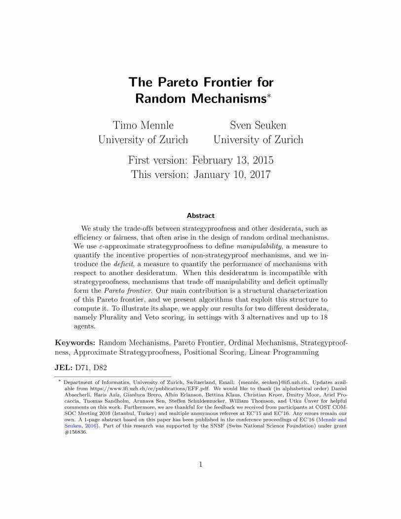
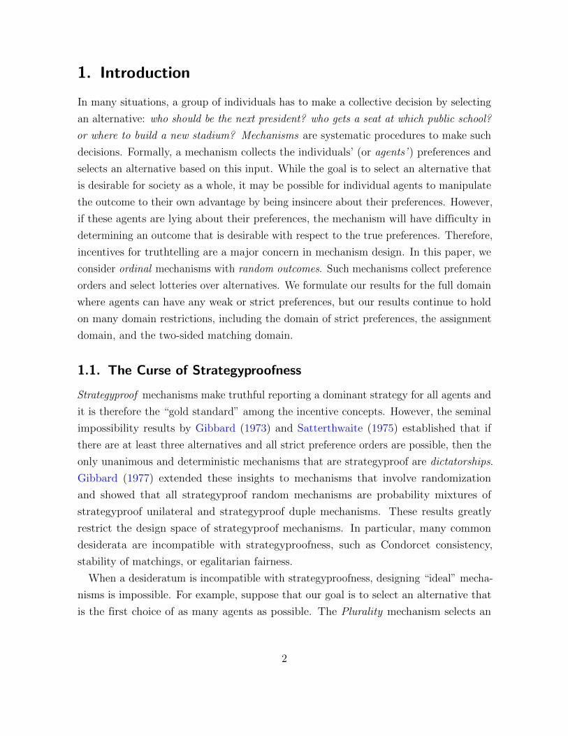
Specifically, the signature of a mechanism ϕ is the point pεpϕq, δpϕqq in the unit square
r0, 1s � r0, 1s. Figure 1 illustrates this comparison. Ideally, a mechanism would be
strategyproof and would always select the most desirable alternatives. This corresponds
to a signature in the origin p0, 0q. However, for desiderata that are incompatible with
strategyproofness, designing ideal mechanisms is not possible. Instead, there exist strate-
gyproof mechanisms which have a non-trivial deficit, such as Random Dictatorship; and
there exist value maximizing mechanisms which have non-trivial manipulability, such as
1Many important desiderata can be expressed via desideratum functions, including binary desideratasuch as unanimity, Condorcet consistency, egalitarian fairness, Pareto optimality, v-rank efficiencyof assignments, stability of matchings, any desideratum specified via a target mechanism (or a targetcorrespondence), or any logical combination of these. Moreover, it is possible to express quantitativedesiderata, such as maximizing positional score in voting, maximizing v-rank value of assignments,or minimizing the number of blocking pairs in matching. We discuss the generality and limitationsof desideratum functions in Section E.
2In the example we considered absolute differences to construct the deficit of outcomes and we consideredthe worst-case deficit to construct the deficit of mechanisms. Alternatively, we can consider relativedifferences and we can also define an ex-ante deficit of mechanisms. Many meaningful notions ofdeficit can be constructed in this way (see Appendix A); the results in this paper hold for any ofthem.
4
0 10
1 ϕ, e.g., RandomDictatorship
ϑ ψ, e.g.,Plurality
Manipulability ε
Def
icitδ
Figure 1: Example signatures of mechanisms in a manipulability-deficit-plot.
Plurality (if the goal is to select an alternative that is the first choice of as many agents
as possible). Finally, there may exist mechanisms that have intermediate signatures,
such as ϑ in Figure 1. Choosing between these mechanisms means to make trade-offs.
Finding Optimal Mechanisms Naturally, we want to make optimal trade-offs. A
mechanism is optimal at manipulability bound ε if it has manipulability of at most ε
and it has the lowest deficit among all such mechanisms. For a given ε we denote by
Optpεq the set of all mechanisms that are optimal at ε. Given an optimal mechanism, it
is not possible to reduce the deficit without increasing manipulability at the same time.
In this sense, the set of all optimal mechanisms constitutes the Pareto frontier. Our
first result yields a finite set of linear constraints that is equivalent to ε-approximate
strategyproofness. This equivalence allows us to formulate the linear program FindOpt,
whose solutions uniquely identify the optimal mechanisms at ε.
Trade-offs via Hybrid Mechanisms Given two mechanisms, mixing them suggests
itself as a natural approach to create new mechanisms with intermediate signatures.
Formally, the β-hybrid of two mechanisms ϕ and ψ is the β-convex combination of
the two mechanisms. Such a hybrid can be implemented by first collecting the agents’
preference reports, then randomly deciding to use ψ or ϕ with probabilities β and 1� β,
respectively. If ϕ has lower manipulability and ψ has lower deficit, then one would
expect their hybrid to inherit a share of both properties. Our second result in this paper
formalizes this intuition: we prove that the signature of a β-hybrid is always weakly
5
preferable on both dimensions to the β-convex combination of the signatures of the two
original mechanisms. This insight teaches us that interesting intermediate mechanisms
can indeed be obtained via mixing.
Our result has important consequences for the Pareto frontier: it implies that the first
unit of manipulability that we sacrifice yields the greatest return in terms of a reduction
of deficit. Furthermore, the marginal return on further relaxing incentive requirements
decreases as the mechanisms become more manipulable. This is good news for mechanism
designers because it means that the most substantial improvements already arise by
relaxing strategyproofness just “a little bit.”
Structural Characterization of the Pareto Frontier To fully understand the possible
and necessary trade-offs between manipulability and deficit, we need to identify the
whole Pareto frontier across all manipulability bounds. Our main result in this paper
is a structural characterization of this Pareto frontier. We show that there exists a
finite set ε0 . . . εK of supporting manipulability bounds, such that between any
two of them (εk�1 and εk, say) the Pareto frontier consists precisely of the hybrids of
two mechanisms that are optimal at εk�1 and εk, respectively. Consequently, the two
building blocks of the Pareto frontier are, first, the optimal mechanisms at the supporting
manipulability bounds εk and, second, the hybrids of optimal mechanisms at adjacent
supporting manipulability bounds for any intermediate ε � εk. Thus, the Pareto frontier
can be represented concisely in terms of a finite number of optimal mechanisms and
their hybrids. In combination with the linear program FindOpt, we can exploit this
characterization to compute the whole Pareto frontier algorithmically.
In summary, we provide a novel perspective on the possible and necessary trade-offs
between incentives and other desiderata. Our results unlock the Pareto frontier of random
mechanisms to analytic, axiomatic, and algorithmic exploration.
2. Related Work
Severe impossibility results restrict the design of strategyproof ordinal mechanisms. The
seminal Gibbard-Satterthwaite Theorem (Gibbard, 1973; Satterthwaite, 1975) established
that if all strict preferences over at least 3 alternatives are possible, then the only
unanimous, strategyproof, and deterministic mechanisms are dictatorial, and Gibbard
6
(1977) extended this result to random mechanisms. Thus, many important desiderata are
incompatible with strategyproofness, such as selecting a Condorcet winner or maximizing
Borda count (Pacuit, 2012). Similar restrictions persist in other domains: in the random
assignment problem, strategyproofness is incompatible with rank efficiency (Featherstone,
2011), and in the two-sided matching problem, strategyproofness is incompatible with
stability (Roth, 1982).
Many research efforts have been made to circumvent these impossibility results and to
obtain better performance on other dimensions. One way to reconcile strategyproofness
with other desiderata is to consider restricted domains. Moulin (1980) showed that in
the single-peaked domain, all strategyproof, anonymous, and efficient mechanisms are
variants of the Median mechanism with additional virtual agents, and Ehlers, Peters and
Storcken (2002) extended this result to random mechanisms. Chatterji, Sanver and Sen
(2013) showed that a semi-single-peaked structure is almost the defining characteristic of
domains that admit the design of strategyproof deterministic mechanisms with appealing
properties; an analogous result for random mechanisms is outstanding.
An alternative way to circumvent impossibility results is to continue working in full
domains but to relax the strategyproofness requirement “a little bit.” This can enable
the design of mechanisms that come closer to achieving a given desideratum but still have
appealing (albeit imperfect) incentive properties. Mennle and Seuken (2017b) introduced
partial strategyproofness, a relaxation of strategyproofness that has particular appeal in
the assignment domain. Azevedo and Budish (2015) proposed strategyproofness in the
large, which requires that the incentives for any individual agent to misreport should
vanish in large markets. However, strategyproofness in the large is unsuited for the exact
analysis of finite settings which we perform in this paper. Instead, we follow Birrell and
Pass (2011) and Carroll (2013), who used approximate strategyproofness for agents with
bounded vNM utility functions to quantify manipulability of non-strategyproof ordinal
mechanisms and derived asymptotic results. We also use approximate strategyproofness
but we give exact results for finite settings.
Some prior work has considered trade-offs explicitly. Using efficiency notions based
on dominance relations, Aziz, Brandt and Brill (2013) and Aziz, Brandl and Brandt
(2014) proved compatibility and incompatibility of various combinations of incentive
and efficiency requirements. Procaccia (2010) considered an approximation ratio based
on positional scoring and gave bounds on how well strategyproof random mechanisms
7
can approximate optimal positional scores as markets get large. While he found most
of these to be inapproximable by strategyproof mechanisms, Birrell and Pass (2011)
obtained positive limit results for the approximation of deterministic target mechanisms
via approximately strategyproof random mechanisms. In (Mennle and Seuken, 2017a)
we studied how hybrid mechanisms make trade-offs between startegyproofness (in terms
of the degree of strategyproofness) and efficiency (in terms of dominance) in random
assignment. While hybrid mechanisms also play a central role in our present paper, we
consider general ordinal mechanisms and different measures (i.e., manipulability and
deficit).
3. Formal Model
Let N be a set of n agents and M be a set of m alternatives, where the tuple pN,Mq
is called a setting. Each agent i P N has a preference order Pi over alternatives, where
Pi : a © b, Pi : a ¡ b, and Pi : a � b denote weak preference, strict preference, and
indifference, respectively, and P denotes the set of all preference orders. For agent i’s
preference order Pi, the rank of alternative j under Pi is the number of alternatives that
i strictly prefers to j plus 1, denoted rankPipjq.3 A preference profile P � pPi, P�iq is
a collection of preference orders from all agents, and P�i are the preference orders of
all other agents, except i. A (random) mechanism is a mapping ϕ : PN Ñ ∆pMq. Here
∆pMq is the space of lotteries over alternatives, and any x P ∆pMq is called an outcome.
We extend agents’ preferences over alternatives to preferences over lotteries via von
Neumann-Morgenstern utility functions: each agent i P N has a utility function ui :
M Ñ r0, 1s that represents their preference order, i.e., uipaq ¥ uipbq holds whenever
Pi : a © b. Note that utility functions are bounded between 0 and 1, so that the model
admits a non-degenerate notion of approximate strategyproofness (see Remark 2). We
denote the set of all utility functions that represent the preference order Pi by UPi .
Remark 1. We formulate our results for the full domain but they naturally extend to a
variety of domains, including the domain of strict preferences, the assignment domain,
and the two-sided matching domain (see Appendix E).
31 is added to ensure that first choice alternatives have rank 1, not 0.
8
4. Approximate Strategyproofness and Manipulability
Our goal in this paper is to study mechanisms that trade off manipulability and other
desiderata optimally. For this purpose we need measures for the performance of different
mechanisms with respect to the two dimensions of this trade-off. In this section, we
review approximate strategyproofness, derive a measure for the incentive properties of
non-strategyproof mechanisms, and present our first main result.
4.1. Strategyproofness and Approximate Strategyproofness
The most demanding incentive concept is strategyproofness. It requires that truthful
reporting is a dominant strategy for all agents. For random mechanisms, this means that
truthful reporting always maximizes any agent’s expected utility.
Definition 1 (Strategyproofness). Given a setting pN,Mq, a mechanism ϕ is strate-
gyproof if for any agent i P N , any preference profile pPi, P�iq P PN , any utility ui P UPithat represents Pi, and any misreport P 1i P P , we have
¸jPM
uipjq � pϕjpP1i , P�iq � ϕjpPi, P�iqq ¤ 0. (1)
The left side of (1) is the change in its own expected utility that i can affect by falsely
reporting P 1i instead of reporting Pi. For later use, we denote this difference by
εpui, pPi, P�iq, P1i , ϕq �
¸jPM
uipjq � pϕjpP1i , P�iq � ϕjpPi, P�iqq . (2)
The fact that εpui, pPi, P�iq, P1i , ϕq is upper bounded by 0 for strategyproof mechanisms
means that deviating from the true preference report weakly decreases expected utility
for any agent in any situation, independent of the other agents’ reports. Conversely, if a
mechanism ϕ is not strategyproof, there necessarily exists at least one situation in which
εpui, pPi, P�iq, P1i , ϕq is strictly positive. Imposing a different bound leads to the notion
of approximate strategyproofness (Birrell and Pass, 2011; Carroll, 2013).
Definition 2 (ε-Approximate Strategyproofness). Given a setting pN,Mq and a bound
ε P r0, 1s, a mechanism ϕ is ε-approximately strategyproof if for any agent i P N ,
9
any preference profile pPi, P�iq P PN , any utility ui P UPi that represents Pi, and any
misreport P 1i P P , we have
εpui, pPi, P�iq, P1i , ϕq �
¸jPM
uipjq � pϕjpP1i , P�iq � ϕjpPi, P�iqq ¤ ε. (3)
This definition is analogous to Definition 1 of strategyproofness, except that the upper
bound in (3) is ε instead of 0. Thus, 0-approximate strategyproofness coincides with
strategyproofness. Furthermore, the gain never exceeds 1, which makes 1-approximate
strategyproofness a void constraint that is trivially satisfied by any mechanism.
The interpretation of intermediate values of ε P p0, 1q is more challenging. Unlike
utilities in quasi-linear domains, vNM utilities are not comparable across agents. Thus,
we cannot simply think of ε as the “value” (e.g., in dollars) that an agent can gain by
misreporting. Instead, ε is a relative bound: since ui is between 0 and 1, a change of
magnitude 1 in expected utility corresponds to the selection of an agent’s first choice
instead of that agent’s last choice. Thus, “1” is the maximal gain from misreporting
that any agent could obtain under an arbitrary mechanism. The bound ε is the share of
this maximal gain by which any agent can at most improve its expected utility under an
ε-approximately strategyproof mechanism.
Remark 2. The bounds on utilities are essential for ε-approximate strategyproofness
to be a useful relaxation of strategyproofness for ordinal mechanisms. Suppose that a
non-strategyproof mechanism ϕ allows a gain of εpui, pPi, P�iq, P1i , ϕq ¡ 0. Then scaling
the utility function ui by a factor α ¡ 1 results in a linear increase of this gain. Thus,
ε-approximate strategyproofness for unbounded utilities would imply strategyproofness.
4.2. Manipulability
If ϕ is ε-approximately strategyproof, then it is also ε1-approximately strategyproof for
any ε1 ¥ ε. Thus, lower values of ε correspond to stronger incentives. With this in mind,
we define the manipulability of a mechanism.
Definition 3 (Manipulability). Given a setting pN,Mq and mechanism ϕ, the manipu-
lability of ϕ (in the setting pN,Mq) is given by
εpϕq � mintε1 P r0, 1s : ϕ is ε1-approximately strategyproof in pN,Mqu. (4)
10

Intuitively, εpϕq is the lowest bound ε1 for which ϕ is ε1-approximately strategyproof.
This minimum is in fact attained because all inequalities from (3) are weak. Note that
in a different setting pN 1,M 1q, the manipulability may vary. However, for all statements
in this paper, a setting is held fixed and the value εpϕq should be understood as the
manipulability of the mechanism ϕ in the fixed setting from the respective context.
4.3. An Equivalent Condition for Approximate Strategyproofness
Recall that the definition of ε-approximate strategyproofness imposes an upper bound
on the gain that agents can obtain by misreporting. In particular, inequality (3) must
hold for all utility functions that represent the agent’s preference order. Since there
are infinitely many such utility functions, a naıve approach to verifying ε-approximate
strategyproofness of a given mechanism would involve checking an infinite number of
constraints. This is somewhat unattractive from an axiomatic perspective and even
prohibitive from an algorithmic perspective. Fortunately, we can bypass this issue, as
the next Theorem 1 shows.
Theorem 1. Given a setting pN,Mq, a bound ε P r0, 1s, and a mechanism ϕ, the
following are equivalent:
1. ϕ is ε-approximately strategyproof in pN,Mq.
2. For any agent i P N , any preference profile pPi, P�iq P PN , any misreport P 1i P P,and any rank r P t1, . . . ,mu, we have
¸jPM :rankPi pjq¤r
ϕjpP1i , P�iq � ϕjpPi, P�iq ¤ ε. (5)
Proof Outline (formal proof in Appendix F.1). The key idea is to represent any utility
function as an element of the convex hull of a certain set of extreme utility functions.
For any combination pi, pPi, P�iq, P1i , kq the inequality in statement (2) is just the ε-
approximate strategyproofness constraints for one extreme utility function.
Theorem 1 yields that ε-approximate strategyproofness can be equivalently expressed
as a finite set of weak, linear inequalities. This has far-reaching consequences. In general,
it unlocks approximate strategyproofness for use under the automated mechanism
11
design paradigm (Sandholm, 2003). Specifically, it enables our identification of optimal
mechanisms as solutions to a particular linear program (Section 6).
5. Desideratum Functions and Deficit
While it is important to elicit truthful preferences, good incentives alone do not make a
mechanism attractive. Instead, it should ultimately select desirable alternatives, where
desirability depends on the agents’ preferences. In this section, we introduce a formal
method to quantify the ability of mechanisms to achieve a given desideratum.
5.1. Desideratum Functions
To express a desideratum formally, we define desideratum functions. These reflect the
value that society derives from selecting a particular alternative when the agents have a
particular preference profile.
Definition 4 (Desideratum Function). A desideratum function is a mapping d : M � PN Ñ r0, 1s,
where dpj,P q is the d-value associated with selecting alternative j when the agents have
preferences P .
We illustrate how desideratum functions represent desiderata with two examples.
Example 1. Suppose that our goal is to select an alternative that is the first choice of
as many agents as possible. We can define the corresponding desideratum function by
setting dPlupj,P q � n1j{n, where n1
j is the number of agents whose first choice under P
is j. Note that dPlupj,P q is proportional to the Plurality score of j under P .
Example 2. Alternatively, we can consider a binary desideratum. An alternative j is
a Condorcet winner at P if it dominates all other alternatives in a pairwise majority
comparison. A mechanism is Condorcet consistent if it selects Condorcet winners
whenever they exist. We can reflect this desideratum by setting dConpj,P q � 1 for any j
that is a Condorcet winner at P , and dConpj,P q � 0 otherwise.
Desideratum functions are extended to (random) outcomes by taking expectations.
12
Definition 5 (Expected d-value). Given a desideratum function d, a preference profile
P P PN , and an outcome x P ∆pMq, the (expected) d-value of x at P is given by
dpx,P q �¸jPM
xj � dpj,P q. (6)
The interpretation of dpx,P q is straightforward: if d quantifies the value of alternatives
(as in Example 1), then dpx,P q is the expectation of the societal value from selecting an
alternative according to x. If d reflects a binary desideratum (as in Example 2), then
dpx,P q is the probability of selecting an alternative with the desirable property.
Remark 3. By taking expectations, the d-value of random outcomes is fully determined
by the d-values of the alternatives. This linear structure is a key ingredient to our
results. In Appendix E, we show that many (but not all) popular desiderata admit such
a representation, and we also discuss the limitations.
Ideally, mechanisms would always select outcomes that maximize the d-value.
Definition 6 (d-maximizing). Given a desideratum function d and a preference profile
P P PN , an outcome x P ∆pMq is d-maximizing at P if dpx,P q � maxjPM dpj,P q. A
mechanism ϕ is d-maximizing if, for any P P PN , ϕpP q is d-maximizing at P .
Note that for any preference profile P there always exists at least one alternative that
is d-maximizing at P by construction. Furthermore, any d-maximizing random outcome
must be a lottery over alternatives that are all d-maximizing at P .
Example 1, continued. Recall the desideratum function dPlupj,P q � n1j{n, where
n1j is the number of agents who ranked j first under P . A mechanism is dPlu-maximizing
if and only if it is a Plurality mechanism (i.e., a mechanism that selects only alternatives
which are the first choice of a maximum number of agents).
Example 2, continued. Recall that dConpj,P q � 1tj Condorcet winners at P u expresses
the desideratum to select Condorcet winners when they exist. Indeed, any dCon-
maximizing mechanism is Condorcet consistent. Moreover, at any preference profile P
where no Condorcet winner exists, the minimal and maximal achievable d-values are
both zero. At these P , the dCon-maximizing mechanisms are therefore free to choose any
outcome. Consequently, maximizing dCon-value is equivalent to Condorcet consistency.
13
5.2. Deficit of Mechanisms
Intuitively, the deficit of an outcome is the loss that society incurs from choosing that
outcome instead of a d-maximizing outcome.
Definition 7 (Deficit of Outcomes). Given a desideratum function d, a preference profile
P P PN , and an outcome x P ∆pMq, the d-deficit of x at P is
δdpx,P q � maxjPM
dpj,P q � dpx,P q. (7)
Remark 4 (Relative Deficit). The difference in (7) is absolute; however, in some situations,
it may be more natural to consider relative differences, such as the ratio between the
achieved and the maximal achievable d-value. As we show in Appendix A.1, it is without
loss of generality that we restrict our attention to absolute differences.
Equipped with the deficit of outcomes, we define the deficit of mechanisms. This
measure is the “desideratum counterpart” to the measure εpϕq for incentive properties.
Definition 8 (Deficit of Mechanisms). Given a setting pN,Mq, a desideratum function
d, and a mechanism ϕ, the (worst-case) d-deficit of ϕ (in pN,Mq) is the highest d-deficit
incurred by ϕ across all preference profiles; formally,
δmaxd pϕq � max
P PPNδdpϕpP q,P q. (8)
Intuitively, the deficit of the mechanism is determined by the most severe violation
of the desideratum across all preference profiles. Thus, a mechanism with low deficit
violates the desideratum only “a little bit” across all possible preference profiles.
Remark 5. Another way to define the deficit of mechanisms arises when agents’ preference
profiles are drawn from a known distribution. In Appendix A.2 we define this ex-ante
deficit formally. All results in this paper hold for both notions of deficit.
For the remainder of this paper, we fix an arbitrary setting pN,Mq, a desideratum
expressed via a desideratum function d, and a notion of deficit δ derived from d. The
triple pN,M, δq is called a problem. Unless explicitly stated otherwise, our results are
understood to hold for any fixed problem pN,M, δq separately.
14
0 10
1
Strategyproof
Ideal d-maximizing
Other
Manipulability ε
Def
icitδ
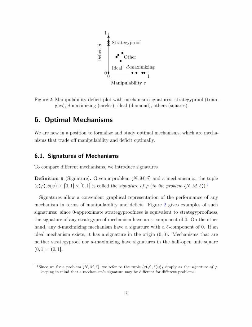
Figure 2: Manipulability-deficit-plot with mechanism signatures: strategyproof (trian-gles), d-maximizing (circles), ideal (diamond), others (squares).
6. Optimal Mechanisms
We are now in a position to formalize and study optimal mechanisms, which are mecha-
nisms that trade off manipulability and deficit optimally.
6.1. Signatures of Mechanisms
To compare different mechanisms, we introduce signatures.
Definition 9 (Signature). Given a problem pN,M, δq and a mechanism ϕ, the tuple
pεpϕq, δpϕqq P r0, 1s � r0, 1s is called the signature of ϕ (in the problem pN,M, δq).4
Signatures allow a convenient graphical representation of the performance of any
mechanism in terms of manipulability and deficit. Figure 2 gives examples of such
signatures: since 0-approximate strategyproofness is equivalent to strategyproofness,
the signature of any strategyproof mechanism have an ε-component of 0. On the other
hand, any d-maximizing mechanism have a signature with a δ-component of 0. If an
ideal mechanism exists, it has a signature in the origin p0, 0q. Mechanisms that are
neither strategyproof nor d-maximizing have signatures in the half-open unit square
p0, 1s � p0, 1s.
4Since we fix a problem pN,M, δq, we refer to the tuple pεpϕq, δpϕqq simply as the signature of ϕ,keeping in mind that a mechanism’s signature may be different for different problems.
15
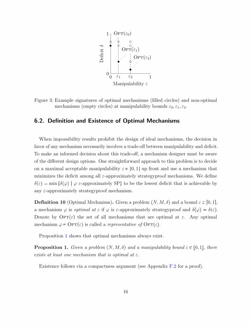
0 ε1 ε2 10
1 Optpε0q
Optpε1q
Optpε2q
Manipulability ε
Def
icitδ
Figure 3: Example signatures of optimal mechanisms (filled circles) and non-optimalmechanisms (empty circles) at manipulability bounds ε0, ε1, ε2.
6.2. Definition and Existence of Optimal Mechanisms
When impossibility results prohibit the design of ideal mechanisms, the decision in
favor of any mechanism necessarily involves a trade-off between manipulability and deficit.
To make an informed decision about this trade-off, a mechanism designer must be aware
of the different design options. One straightforward approach to this problem is to decide
on a maximal acceptable manipulability ε P r0, 1s up front and use a mechanism that
minimizes the deficit among all ε-approximately strategyproof mechanisms. We define
δpεq � min tδpϕq | ϕ ε-approximately SPu to be the lowest deficit that is achievable by
any ε-approximately strategyproof mechanism.
Definition 10 (Optimal Mechanism). Given a problem pN,M, δq and a bound ε P r0, 1s,
a mechanism ϕ is optimal at ε if ϕ is ε-approximately strategyproof and δpϕq � δpεq.
Denote by Optpεq the set of all mechanisms that are optimal at ε. Any optimal
mechanism ϕ P Optpεq is called a representative of Optpεq.
Proposition 1 shows that optimal mechanisms always exist.
Proposition 1. Given a problem pN,M, δq and a manipulability bound ε P r0, 1s, there
exists at least one mechanism that is optimal at ε.
Existence follows via a compactness argument (see Appendix F.2 for a proof).
16
Proposition 1 justifies the use of the minimum (rather than the infimum) in the defini-
tion of δpεq, since the deficit δpεq � δpϕq is in fact attained by some mechanism. Figure
3 illustrates signatures of optimal and non-optimal mechanisms. On the vertical lines at
each of the manipulability bounds ε0 � 0, ε1, ε2, the circles (empty circles) correspond to
signatures of non-optimal mechanisms. The signatures of optimal mechanisms (filled
circles) from Optpεkq, k � 0, 1, 2 take the lowest positions on the vertical lines.
6.3. Identifying Optimal Mechanisms
The existence proof for optimal mechanisms is implicit and does not provide a way of
actually determining them. Our next result establishes a correspondence between the
set Optpεq and the set of solutions to a linear program. We can solve this program
algorithmically to find representatives of Optpεq and to compute δpεq.
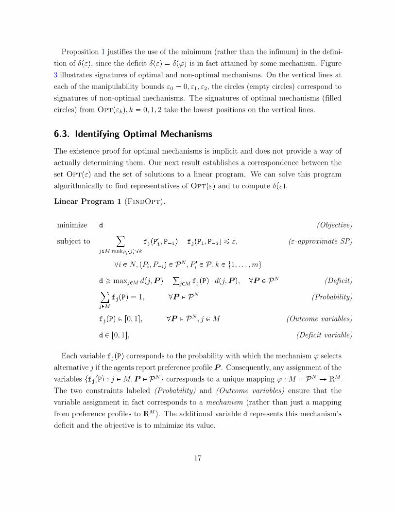
Linear Program 1 (FindOpt).
minimize d (Objective)
subject to¸
jPM :rankPi pjq¤k
fjpP1i, P�iq � fjpPi, P�iq ¤ ε, (ε-approximate SP)
@i P N, pPi, P�iq P PN , P 1i P P , k P t1, . . . ,mu
d ¥ maxjPM dpj,P q �°jPM fjpPq � dpj,P q, @P P PN (Deficit)¸
jPM
fjpPq � 1, @P P PN (Probability)
fjpPq P r0, 1s, @P P PN , j PM (Outcome variables)
d P r0, 1s, (Deficit variable)
Each variable fjpPq corresponds to the probability with which the mechanism ϕ selects
alternative j if the agents report preference profile P . Consequently, any assignment of the
variables tfjpPq : j PM,P P PNu corresponds to a unique mapping ϕ : M � PN Ñ RM .
The two constraints labeled (Probability) and (Outcome variables) ensure that the
variable assignment in fact corresponds to a mechanism (rather than just a mapping
from preference profiles to RM). The additional variable d represents this mechanism’s
deficit and the objective is to minimize its value.
17
The constraints labeled (ε-approximate SP) reflect the equivalent condition for ε-
approximate strategyproofness that we obtained from Theorem 1. In combination, these
constraints ensure that the mechanisms corresponding to the feasible variable assignments
of FindOpt are exactly the ε-approximately strategyproof mechanisms. The constraint
labeled (Deficit) makes d an upper bound for the deficit of ϕ.5
The following Proposition 2 formalizes the correspondence between optimal mechanisms
and solutions of the linear program FindOpt.
Proposition 2. Given a problem pN,M, δq and a bound ε P r0, 1s, a variable assignment
tfjpPq : j PM,P P PNu is a solution of FindOpt at ε if and only if the mechanism ϕ
defined by ϕjpP q � fjpPq for all j PM,P P PN is optimal at ε.
The proof follows directly from the discussion above. One important consequence
of Proposition 2 is that we can compute optimal mechanisms for any given problem
pN,M, δq and any manipulability bound ε P r0, 1s. Going back to the mechanism
designer’s problem of trading off manipulability and deficit, we now have a way of
determining optimal mechanisms for particular manipulability bounds ε. With FindOpt
we can evaluate algorithmically what deficit we must accept when manipulability must
not exceed some fixed limit ε.
Shifting the burden of design to a computer by encoding good mechanisms in optimiza-
tion problems is the central idea of automated mechanism design (Sandholm, 2003). A
common challenge with this approach is that the optimization problem can become large
and difficult to solve; and naıve implementations of FindOpt will face this issue as well.
Substantial run-time improvements are possible, e.g., by exploiting additional axioms
such as anonymity and neutrality (Mennle, Abaecherli and Seuken, 2015). Nonetheless,
determining optimal mechanisms remains a computationally expensive operation.
Computational considerations aside, Proposition 2 provides a new understanding of
optimal mechanisms: since Optpεq corresponds to the solutions of the linear program
FindOpt, it can be interpreted as a convex polytope. In Section 8 we use methods
from convex geometry to derive our structural characterization of the Pareto frontier.
The representation of optimal mechanisms as solutions to FindOpt constitutes the first
building block of this characterization.
5Alternatively, we can implement the ex-ante deficit by replacing the (Deficit)-constraint (see AppendixA.2).
18
7. Hybrid Mechanisms
In this section, we introduce hybrid mechanisms, which are convex combinations of two
component mechanisms. Intuitively, by mixing one mechanism with low manipulability
and another mechanism with low deficit, we may hope to obtain new mechanisms with
intermediate signatures. Initially, the construction of hybrids is independent of the study
of optimal mechanisms. However, in Section 8, they will constitute the second building
block for our structural characterization of the Pareto frontier.
Definition 11 (Hybrid). For β P r0, 1s and mechanisms ϕ and ψ, the β-hybrid hβ is
given by hβpP q � p1� βqϕpP q � βψpP q for any preference profile P P PN .
In practice, “running” a hybrid mechanism is straightforward: first, collect the prefer-
ence reports. Second, toss a β-coin to determine whether to use ψ (probability β) or ϕ
(probability 1� β). Third, apply this mechanism to the reported preference profile. Our
next result formalizes the intuition that hybrids have at least intermediate signatures.
Theorem 2. Given a problem pN,M, δq, mechanisms ϕ, ψ, and β P r0, 1s, we have
εphβq ¤ p1� βqεpϕq � βεpψq, (9)
δphβq ¤ p1� βqδpϕq � βδpψq. (10)
Proof Outline (formal proof in Appendix F.3). We write out the definitions of εphβq and
δphβq, each of which may involve taking a maximum. The two inequalities are then
obtained with the help of the triangle inequality.
In words, the signatures of β-hybrids are always weakly better than the β-convex
combination of the signatures of the two component mechanisms.
There are two important takeaways from Theorem 2. First, it yields a strong argument
in favor of randomization: given two mechanisms with attractive manipulability and
deficit, randomizing between the two always yields a mechanism with a signature that is
at least as attractive as the β-convex combination of the signatures of the two mechanisms.
As Example 3 in Appendix B shows, randomizing in this way can yield strictly preferable
mechanisms that have strictly lower manipulability and strictly lower deficit than either
of the component mechanisms.
19
The second takeaway is that the common fairness requirement of anonymity comes “for
free” in terms of manipulability and deficit (provided that the deficit measure δ is itself
anonymous): given any mechanism ϕ, an anonymous mechanism can be constructed by
randomly assigning the agents to new roles. This yields a hybrid mechanism with many
components, each of which corresponds to the original mechanism with agents assigned
to different roles. Under an anonymous deficit notion, every component will have the
same signature as ϕ. If follows from Theorem 2 that this new anonymous mechanism has
a weakly better signature than ϕ. Similarly, we can impose neutrality without having to
accept higher manipulability or more deficit (if δ is itself neutral). We formalize these
insights in Appendix C.
8. The Pareto Frontier
Recall that optimal mechanisms are those mechanisms that trade off manipulability and
deficit optimally. They form the Pareto frontier because we cannot achieve a strictly
lower deficit without accepting strictly higher manipulability.
Definition 12 (Pareto Frontier). Given a problem pN,M, δq, let ε be the smallest
manipulability bound that is compatible with d-maximization; formally,
ε � mintε P r0, 1s | Dϕ : ϕ d-maximizing & ε-approximately SPu. (11)
The Pareto frontier is the union of all mechanisms that are optimal for some manipula-
bility bound ε P r0, εs; formally,
Pf �¤
εPr0,εs
Optpεq. (12)
The special manipulability bound ε is chosen such that maximal d-value can be
achieved with an ε-approximately strategyproof mechanisms (ϕ, say) but not with any
mechanism that has strictly lower manipulability. Since ϕ has deficit 0, any mechanism
ϕ that is optimal at some larger manipulability bound ε ¡ ε may be more manipulable
than ϕ but ϕ cannot have a strictly lower deficit. Thus, we can restrict attention to
manipulability bounds between 0 and ε (instead of 0 and 1). From the perspective of
the mechanism designer, mechanisms on the Pareto frontier are the only mechanisms
20
that should be considered; if a mechanism is not on the Pareto frontier, we can find
another mechanism that is a Pareto-improvement in the sense that it has strictly lower
manipulability, strictly lower deficit, or both.
8.1. Monotonicity and Convexity
Recall that we have defined δpεq as the smallest deficit that can be attained by any
ε-approximately strategyproof mechanism. Thus, the signatures of mechanisms on the
Pareto frontier are described by the mapping ε ÞÑ δpεq that associates each manipulability
bound ε P r0, εs with the deficit δpεq of optimal mechanisms at this manipulability bound.
Based on our results so far, we can already make interesting observations about the
Pareto frontier by analyzing this mapping.
Corollary 1. Given a problem pN,M, δq, the mapping ε ÞÑ δpεq is monotonically
decreasing and convex.
Monotonicity follows from the definition of optimal mechanisms, and convexity is a
consequence of Theorem 2 (see Appendix F.4 for a formal proof). While monotonicity
is merely reassuring, convexity is non-trivial and very important. It means that when
we relax strategyproofness, the first unit of manipulability that we give up allows the
largest reduction of deficit. For any additional unit of manipulability that we sacrifice,
the deficit will be reduced at a lower rate, which means decreasing marginal returns.
Thus, we can expect to capture most gains in d-value from relaxing strategyproofness
early on. Moreover, convexity and monotonicity together imply continuity. This means
that trade-offs along the Pareto frontier are smooth in the sense that a tiny reduction of
the manipulability bound ε does not require accepting a vastly higher deficit.
For mechanism designers, these observations deliver an important lesson: the most
substantial gains (per unit of manipulability) arise from relaxing strategyproofness just
“a little bit.” This provides encouragement to investigate the gains from accepting even
small amounts of manipulability. On the other hand, if the initial gains are not worth
the sacrifice, then gains from accepting more manipulability will not be “surprisingly”
attractive either.
21
8.2. A Structural Characterization of the Pareto Frontier
In Section 6, we have shown that we can identify optimal mechanisms for individual
manipulability bounds by solving the linear program FindOpt. In Section 7, we have
introduced hybrids, and we have shown how mixing two mechanisms results in new
mechanisms with intermediate or even superior signatures. We now give our main result,
a structural characterization of the Pareto frontier in terms of these two building blocks,
namely optimal mechanisms and hybrids.
Theorem 3. Given a problem pN,M, δq, there exists a finite set of supporting manipu-
lability bounds
ε0 � 0 ε1 . . . εK�1 εK � ε, (13)
such that for any k P t1, . . . , Ku and any ε P rεk�1, εks with β �ε�εk�1
εk�εk�1we have that
Optpεq � p1� βqOptpεk�1q � βOptpεkq, (14)
δpεq � p1� βqδpεk�1q � βδpεkq. (15)
Proof Outline (formal proof in Appendix F.5). Our proof exploits that Optpεq corre-
sponds to the solutions of the linear program FindOpt (Section 6.3) with feasible set
Fε � tx |Dx ¤ d,Ax ¤ εu, where neither D, nor d, nor A depend on ε. First, we show
that if a set of constraints is binding for Fε, then it is binding for Fε1 for ε1 within a
compact interval rε�, ε�s that contains ε and not binding for any ε2 R rε�, ε�s. With
finiteness of the number of constraints of the LP, this yields a finite segmentation of
r0, εs. The vertex-representations (Grunbaum, 2003) can then be used to show that
on each segment rεk�1, εks, the solution sets Sε � argminFε d are exactly the β-convex
combinations of Sεk�1and Sεk with β � ε�εk�1
εk�εk�1.
It would be particularly simple if the optimal mechanisms at some manipulability
bound ε were just the β-hybrids of optimal mechanisms at 0 and ε with β � ε{ε. While
this is not true in general, Theorem 3 shows that the Pareto frontier has a linear structure
over each interval rεk�1, εks. Thus, it is completely identified by two building blocks: (1)
the sets of optimal mechanisms Optpεkq for finitely many εk, k � 0, . . . , K, and (2) hybrid
mechanisms, which provide the missing link for ε � εk. Representatives of Optpεkq can
be obtained by solving the linear program FindOpt at the supporting manipulability
22
0 ε1 ε2 10
1
ϕ1 P Optpε1q
hβ P Optpp1� βqε1 � βε2q
ϕ2 P Optpε2q
Manipulability ε
Def
icitδP
lu
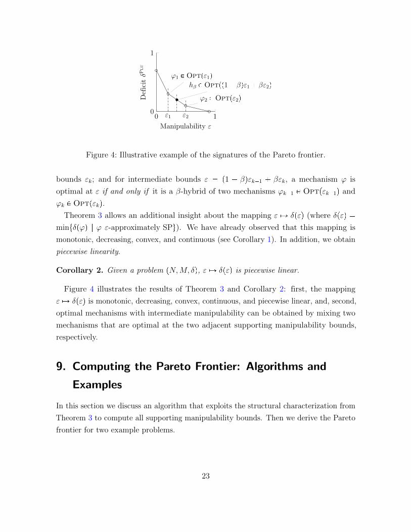
Figure 4: Illustrative example of the signatures of the Pareto frontier.
bounds εk; and for intermediate bounds ε � p1 � βqεk�1 � βεk, a mechanism ϕ is
optimal at ε if and only if it is a β-hybrid of two mechanisms ϕk�1 P Optpεk�1q and
ϕk P Optpεkq.
Theorem 3 allows an additional insight about the mapping ε ÞÑ δpεq (where δpεq �
mintδpϕq | ϕ ε-approximately SPu). We have already observed that this mapping is
monotonic, decreasing, convex, and continuous (see Corollary 1). In addition, we obtain
piecewise linearity.
Corollary 2. Given a problem pN,M, δq, ε ÞÑ δpεq is piecewise linear.
Figure 4 illustrates the results of Theorem 3 and Corollary 2: first, the mapping
ε ÞÑ δpεq is monotonic, decreasing, convex, continuous, and piecewise linear, and, second,
optimal mechanisms with intermediate manipulability can be obtained by mixing two
mechanisms that are optimal at the two adjacent supporting manipulability bounds,
respectively.
9. Computing the Pareto Frontier: Algorithms and
Examples
In this section we discuss an algorithm that exploits the structural characterization from
Theorem 3 to compute all supporting manipulability bounds. Then we derive the Pareto
frontier for two example problems.
23
9.1. Algorithm FindBounds
Recall that the linear program FindOpt can be used to determine a representative of the
set of optimal mechanisms Optpεq. One naıve approach to identifying the Pareto frontier
would be to run FindOpt for many different manipulability bounds to obtain optimal
mechanisms at each of these bounds, and then consider these mechanisms and their
hybrids. However, this method has two drawbacks: first, and most importantly, it would
not yield the correct Pareto frontier. The result can, at best, be viewed as a conservative
estimate, since choosing fixed manipulability bounds is not guaranteed to identify
any actual supporting manipulability bounds exactly. Second, from a computational
perspective, executing FindOpt is expensive, which is why we would like to keep the
number of executions as low as possible.
Knowing the structure of the Pareto frontier, we can use the information obtained
from iterated applications of FindOpt to interpolate the most promising candidates
for supporting manipulability bounds. In Appendix D we provide the algorithms
FindBounds (Algorithm 1) and FindLower (Algorithm 2) that do this. Proposition
3 summarizes their properties.
Proposition 3. Given a problem pN,M, δq, the algorithms FindLower and Find-
Bounds require at most 4K � log2 p1{ε1q � 1 executions of the linear program FindOpt
to determine all supporting manipulability bounds of the Pareto frontier, where K is the
number of supporting manipulability bounds and ε1 is the smallest non-trivial supporting
manipulability bound.
Due to space constraints we delegate the detailed discussion of the algorithms and the
proof of Proposition 3 to Appendix D.
9.2. Examples: Plurality Scoring and Veto Scoring
In this section, we consider two concrete problems and derive the respective Pareto
frontiers. The two examples highlight the different shapes that the Pareto frontier can
take. Both settings contain 3 alternatives and 3 agents with strict preferences over the
alternatives, but they differ in the desideratum.
24
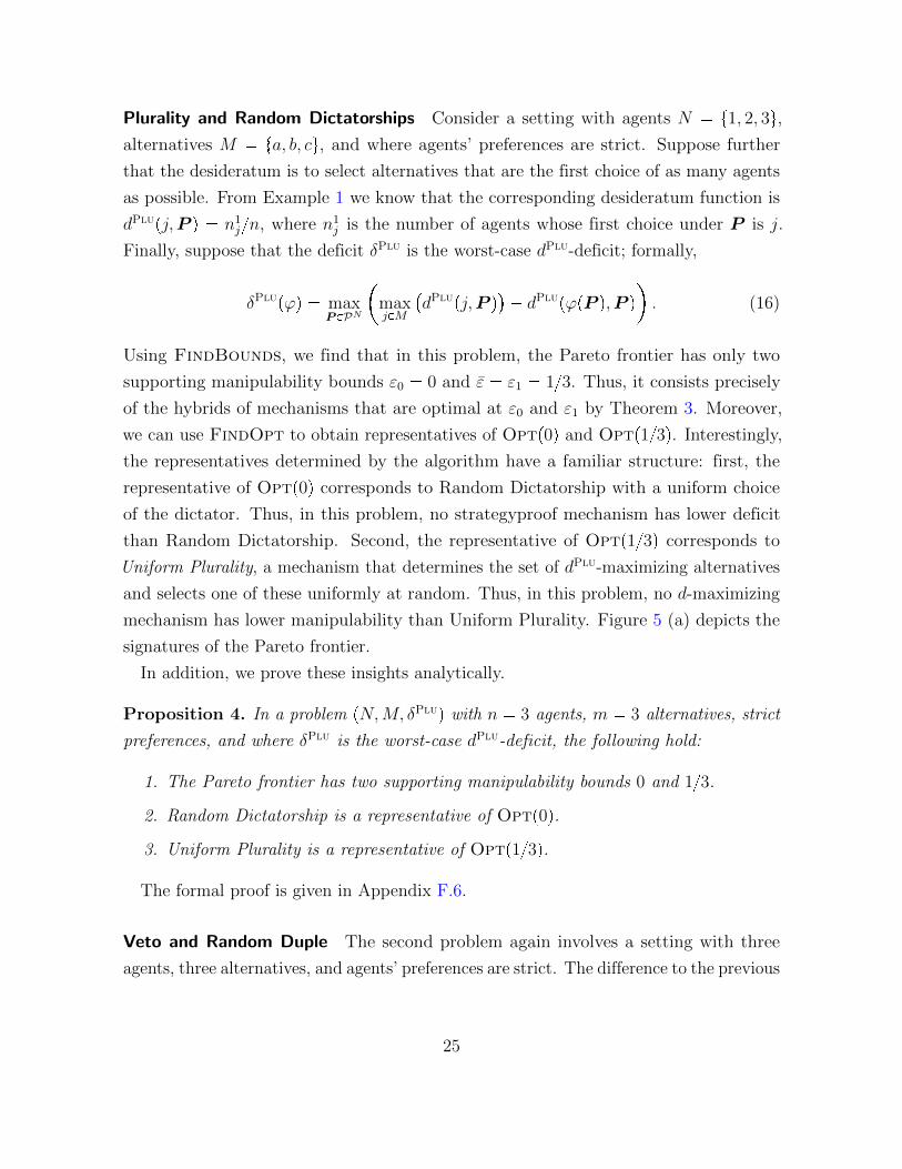
Plurality and Random Dictatorships Consider a setting with agents N � t1, 2, 3u,
alternatives M � ta, b, cu, and where agents’ preferences are strict. Suppose further
that the desideratum is to select alternatives that are the first choice of as many agents
as possible. From Example 1 we know that the corresponding desideratum function is
dPlupj,P q � n1j{n, where n1
j is the number of agents whose first choice under P is j.
Finally, suppose that the deficit δPlu is the worst-case dPlu-deficit; formally,
δPlupϕq � maxP PPN
�maxjPM
�dPlupj,P q
�� dPlupϕpP q,P q
. (16)
Using FindBounds, we find that in this problem, the Pareto frontier has only two
supporting manipulability bounds ε0 � 0 and ε � ε1 � 1{3. Thus, it consists precisely
of the hybrids of mechanisms that are optimal at ε0 and ε1 by Theorem 3. Moreover,
we can use FindOpt to obtain representatives of Optp0q and Optp1{3q. Interestingly,
the representatives determined by the algorithm have a familiar structure: first, the
representative of Optp0q corresponds to Random Dictatorship with a uniform choice
of the dictator. Thus, in this problem, no strategyproof mechanism has lower deficit
than Random Dictatorship. Second, the representative of Optp1{3q corresponds to
Uniform Plurality, a mechanism that determines the set of dPlu-maximizing alternatives
and selects one of these uniformly at random. Thus, in this problem, no d-maximizing
mechanism has lower manipulability than Uniform Plurality. Figure 5 (a) depicts the
signatures of the Pareto frontier.
In addition, we prove these insights analytically.
Proposition 4. In a problem pN,M, δPluq with n � 3 agents, m � 3 alternatives, strict
preferences, and where δPlu is the worst-case dPlu-deficit, the following hold:
1. The Pareto frontier has two supporting manipulability bounds 0 and 1{3.
2. Random Dictatorship is a representative of Optp0q.
3. Uniform Plurality is a representative of Optp1{3q.
The formal proof is given in Appendix F.6.
Veto and Random Duple The second problem again involves a setting with three
agents, three alternatives, and agents’ preferences are strict. The difference to the previous
25
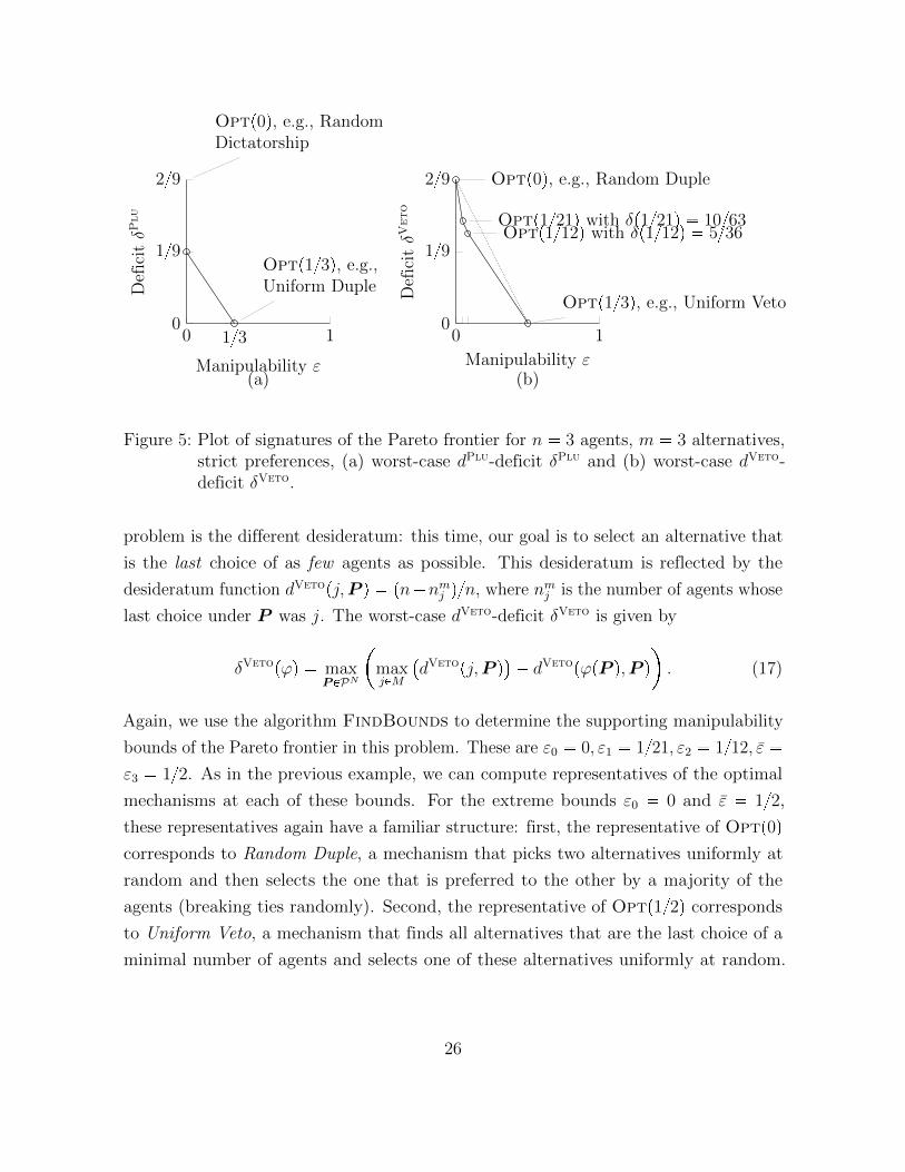
0 1{3 10
1{9
2{9
Optp0q, e.g., RandomDictatorship
Optp1{3q, e.g.,Uniform Duple
Manipulability ε
Def
icitδP
lu
0 10
1{9
2{9 Optp0q, e.g., Random Duple
Optp1{21q with δp1{21q � 10{63Optp1{12q with δp1{12q � 5{36
Optp1{3q, e.g., Uniform Veto
Manipulability ε
Def
icitδV
eto
(a) (b)
Figure 5: Plot of signatures of the Pareto frontier for n � 3 agents, m � 3 alternatives,strict preferences, (a) worst-case dPlu-deficit δPlu and (b) worst-case dVeto-deficit δVeto.
problem is the different desideratum: this time, our goal is to select an alternative that
is the last choice of as few agents as possible. This desideratum is reflected by the
desideratum function dVetopj,P q � pn�nmj q{n, where nmj is the number of agents whose
last choice under P was j. The worst-case dVeto-deficit δVeto is given by
δVetopϕq � maxP PPN
�maxjPM
�dVetopj,P q
�� dVetopϕpP q,P q
. (17)
Again, we use the algorithm FindBounds to determine the supporting manipulability
bounds of the Pareto frontier in this problem. These are ε0 � 0, ε1 � 1{21, ε2 � 1{12, ε �
ε3 � 1{2. As in the previous example, we can compute representatives of the optimal
mechanisms at each of these bounds. For the extreme bounds ε0 � 0 and ε � 1{2,
these representatives again have a familiar structure: first, the representative of Optp0q
corresponds to Random Duple, a mechanism that picks two alternatives uniformly at
random and then selects the one that is preferred to the other by a majority of the
agents (breaking ties randomly). Second, the representative of Optp1{2q corresponds
to Uniform Veto, a mechanism that finds all alternatives that are the last choice of a
minimal number of agents and selects one of these alternatives uniformly at random.
26
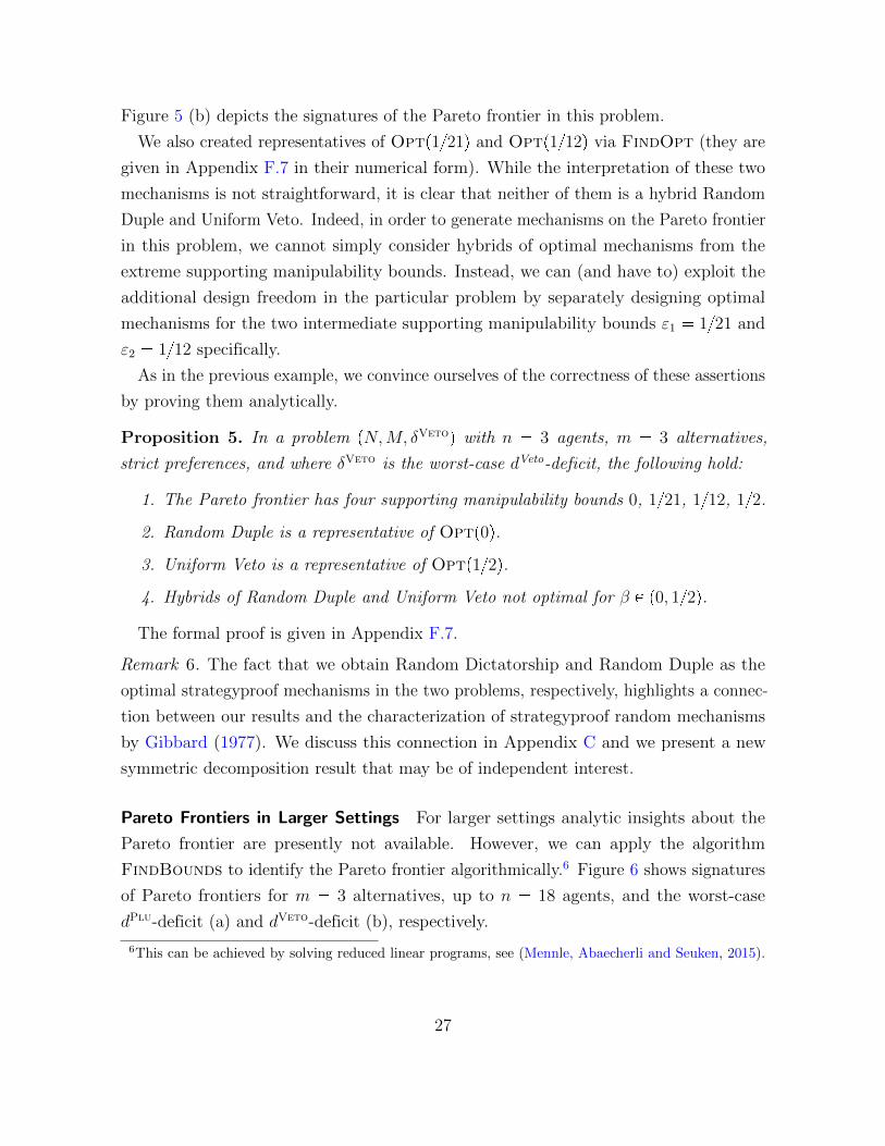
Figure 5 (b) depicts the signatures of the Pareto frontier in this problem.
We also created representatives of Optp1{21q and Optp1{12q via FindOpt (they are
given in Appendix F.7 in their numerical form). While the interpretation of these two
mechanisms is not straightforward, it is clear that neither of them is a hybrid Random
Duple and Uniform Veto. Indeed, in order to generate mechanisms on the Pareto frontier
in this problem, we cannot simply consider hybrids of optimal mechanisms from the
extreme supporting manipulability bounds. Instead, we can (and have to) exploit the
additional design freedom in the particular problem by separately designing optimal
mechanisms for the two intermediate supporting manipulability bounds ε1 � 1{21 and
ε2 � 1{12 specifically.
As in the previous example, we convince ourselves of the correctness of these assertions
by proving them analytically.
Proposition 5. In a problem pN,M, δVetoq with n � 3 agents, m � 3 alternatives,
strict preferences, and where δVeto is the worst-case dVeto-deficit, the following hold:
1. The Pareto frontier has four supporting manipulability bounds 0, 1{21, 1{12, 1{2.
2. Random Duple is a representative of Optp0q.
3. Uniform Veto is a representative of Optp1{2q.
4. Hybrids of Random Duple and Uniform Veto not optimal for β P p0, 1{2q.
The formal proof is given in Appendix F.7.
Remark 6. The fact that we obtain Random Dictatorship and Random Duple as the
optimal strategyproof mechanisms in the two problems, respectively, highlights a connec-
tion between our results and the characterization of strategyproof random mechanisms
by Gibbard (1977). We discuss this connection in Appendix C and we present a new
symmetric decomposition result that may be of independent interest.
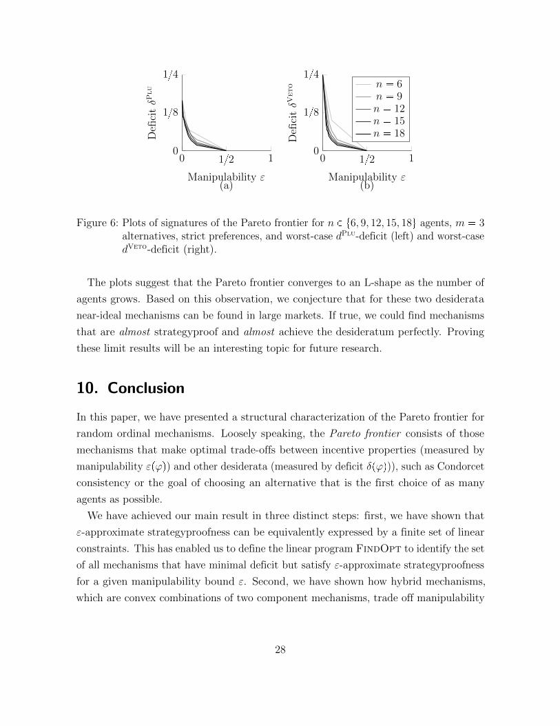
Pareto Frontiers in Larger Settings For larger settings analytic insights about the
Pareto frontier are presently not available. However, we can apply the algorithm
FindBounds to identify the Pareto frontier algorithmically.6 Figure 6 shows signatures
of Pareto frontiers for m � 3 alternatives, up to n � 18 agents, and the worst-case
dPlu-deficit (a) and dVeto-deficit (b), respectively.
6This can be achieved by solving reduced linear programs, see (Mennle, Abaecherli and Seuken, 2015).
27
0 1{2 10
1{8
1{4
Manipulability ε
Def
icitδP
lu
0 1{2 10
1{8
1{4
Manipulability ε
Def
icitδV
eto n � 6
n � 9n � 12n � 15n � 18
(a) (b)
Figure 6: Plots of signatures of the Pareto frontier for n P t6, 9, 12, 15, 18u agents, m � 3alternatives, strict preferences, and worst-case dPlu-deficit (left) and worst-casedVeto-deficit (right).
The plots suggest that the Pareto frontier converges to an L-shape as the number of
agents grows. Based on this observation, we conjecture that for these two desiderata
near-ideal mechanisms can be found in large markets. If true, we could find mechanisms
that are almost strategyproof and almost achieve the desideratum perfectly. Proving
these limit results will be an interesting topic for future research.
10. Conclusion
In this paper, we have presented a structural characterization of the Pareto frontier for
random ordinal mechanisms. Loosely speaking, the Pareto frontier consists of those
mechanisms that make optimal trade-offs between incentive properties (measured by
manipulability εpϕq) and other desiderata (measured by deficit δpϕq)), such as Condorcet
consistency or the goal of choosing an alternative that is the first choice of as many
agents as possible.
We have achieved our main result in three distinct steps: first, we have shown that
ε-approximate strategyproofness can be equivalently expressed by a finite set of linear
constraints. This has enabled us to define the linear program FindOpt to identify the set
of all mechanisms that have minimal deficit but satisfy ε-approximate strategyproofness
for a given manipulability bound ε. Second, we have shown how hybrid mechanisms,
which are convex combinations of two component mechanisms, trade off manipulability
28
and deficit. In particular, we have given a guarantee that the signature of a β-hybrid
hβ is always at least as good as the β-convex combination of the signatures of the two
component mechanisms. Third, we have shown that the Pareto frontier consists of
two building blocks: (1) there exists a finite set of supporting manipulability bounds
ε0, . . . , εK such that we can characterize the set of optimal mechanisms at each of the
bounds εk as the set of solutions to the linear program FindOpt at εk, and (2) for any
intermediate manipulability bound ε � p1� βqεk�1 � βεk, the set of optimal mechanisms
at ε is precisely the set of β-hybrids of optimal mechanisms at each of the two adjacent
supporting manipulability bounds εk�1 and εk.
Our results have a number of interesting consequences (beyond their relevance in this
paper): first, Theorem 1 gives a finite set of linear constraints that is equivalent to
ε-approximate strategyproofness. This makes ε-approximate strategyproofness accessible
to algorithmic analysis. In particular, it enables the use of this incentive requirement
under the automated mechanism design paradigm.
Second, the performance guarantees for hybrid mechanisms from Theorem 2 yield
convincing arguments in favor of randomization. In particular, we learn that the
important requirements of anonymity and neutrality come “for free;” mechanism designers
do not have to accept a less desirable signature when imposing either or both (provided
that the deficit measure is anonymous, neutral, or both).
Third, our main result, Theorem 3, has provided a structural understanding of the
whole Pareto frontier. Knowledge of the Pareto frontier enables mechanism designers
to make a completely informed decision about trade-offs between manipulability and
deficit. In particular, we now have a way to determine precisely by how much the
performance of mechanisms (with respect to a given desideratum) can be improved when
allowing additional manipulability. An important learning is that the mapping ε ÞÑ δpεq,
which associates each manipulability bound with the lowest achievable deficit at this
manipulability bound, is monotonic, decreasing, convex, continuous, and piecewise linear.
This means that when trading off manipulability and deficit along the Pareto frontier,
the trade-offs are smooth, and the earliest sacrifices yield the greatest gains. Thus, it
can be worthwhile to consider even small bounds ε ¡ 0 in order to obtain substantial
improvements.
Finally, we have illustrated our results by considering two concrete problems. In
both problems, three agents had strict preferences over three alternatives. In the first
29
problem, the desideratum was to choose an alternative that is the first choice of as many
agents as possible (i.e., Plurality scoring), and in the second problem, the desideratum
was to choose an alternative that is the last choice of as few agents as possible (i.e.,
Veto scoring). In both problems, we have computed the Pareto frontier and verified
the resulting structure analytically. The examples have shown that the Pareto frontier
may be completely linear (first problem) or truly non-linear (second problem). For
the same desiderata and up to n � 18 agents we have determined the Pareto frontier
algorithmically and formulated a conjecture about its limit behavior.
In summary, we have given novel insights about the Pareto frontier for random ordinal
mechanisms. We have proven our results for the full ordinal domain that includes
indifferences, but they continue to hold for many other interesting domains that arise by
restricting the space of preference profiles, such as the assignment domain and the two-
sided matching domain. When impossibility results restrict the design of strategyproof
mechanisms, we have provided a new perspective on the unavoidable trade-off between
incentives and other desiderata along this Pareto frontier.
References
Abdulkadiroglu, Atila, and Tayfun Sonmez. 2003. “School Choice: A Mechanism Design
Approach.” American Economic Review, 93(3): 729–747.
Azevedo, Eduardo, and Eric Budish. 2015. “Strategy-proofness in the Large.” Working
Paper.
Aziz, Haris, Felix Brandt, and Markus Brill. 2013. “On the Tradeoff Between Economic
Efficiency and Strategy Proofness in Randomized Social Choice.” In Proceedings of the 2013
International Conference on Autonomous Agents and Multi-agent Systems (AAMAS).
Aziz, Haris, Florian Brandl, and Felix Brandt. 2014. “On the Incompatibility of Ef-
ficiency and Strategyproofness in Randomized Social Choice.” In Proceedings of the 28th
Conference on Artificial Intelligence (AAAI).
Birrell, Eleanor, and Rafael Pass. 2011. “Approximately Strategy-Proof Voting.” In
Proceedings of the 22nd International Joint Conference on Artificial Intelligence (IJCAI).
30
Budish, Eric. 2011. “The Combinatorial Assignment Problem: Approximate Competitive
Equilibrium from Equal Incomes.” Journal of Political Economy, 119(6): 1061–1103.
Carroll, Garbiel. 2013. “A Quantitative Approach to Incentives: Application to Voting
Rules.” Working Paper.
Chatterji, Shurojit, Remzi Sanver, and Arunava Sen. 2013. “On Domains that Ad-
mit Well-behaved Strategy-proof Social Choice Functions.” Journal of Economic Theory,
148(3): 1050–1073.
Ehlers, Lars, Hans Peters, and Ton Storcken. 2002. “Strategy-Proof Probabilistic Deci-
sion Schemes for One-Dimensional Single-Peaked Preferences.” Journal of Economic Theory,
105(2): 408–434.
Featherstone, Clayton. 2011. “A Rank-based Refinement of Ordinal Efficiency and a new
(but Familiar) Class of Ordinal Assignment Mechanisms.” Working Paper.
Gibbard, Allan. 1973. “Manipulation of Voting Schemes: a General Result.” Econometrica,
41(4): 587–601.
Gibbard, Allan. 1977. “Manipulation of Schemes That Mix Voting with Chance.” Economet-
rica, 45(3): 665–81.
Grunbaum, Branko. 2003. Convex Polytopes. Graduate Texts in Mathematics. 2 ed., Springer.
Mennle, Timo, and Sven Seuken. 2016. “The Pareto Frontier for Random Mechanisms
[Extended Abstract].” In Proceedings of the 17th ACM Conference on Economics and
Computation (EC).
Mennle, Timo, and Sven Seuken. 2017a. “Hybrid Mechanisms: Trading Off Strategyproof-
ness and Efficiency of Random Assignment Mechanisms.” Working Paper.
Mennle, Timo, and Sven Seuken. 2017b. “Partial Strategyproofness: Relaxing Strate-
gyproofness for the Random Assignment Problem.” Working Paper.
Mennle, Timo, Daniel Abaecherli, and Sven Seuken. 2015. “Computing Pareto Frontier
for Randomized Mechanisms.” Mimeo.
Moulin, Herve. 1980. “On Strategy-Proofness and Single Peakedness.” Public Choice,
35(4): 437–455.
31
Pacuit, Eric. 2012. “Voting Methods.” In The Stanford Encyclopedia of Philosophy. Winter
2012 ed., ed. Edward Zalta. Stanford University.
Procaccia, Ariel. 2010. “Can Approximation Circumvent Gibbard-Satterthwaite?” In Pro-
ceedings of the 24th Conference on Artificial Intelligence (AAAI).
Procaccia, Ariel, and Jeffrey Rosenschein. 2006. “The Distortion of Cardinal Preferences
in Voting.” In Cooperative Information Agents X. Vol. 4149 of Lecture Notes in Computer
Science, ed. Matthias Klusch, Michael Rovatsos and Terry Payne, 317–331. Springer.
Roth, Alvin. 1982. “The Economics of Matching: Stability and Incentives.” Mathematical
Operations Research, 7: 617–628.
Roth, Alvin. 1984. “The Evolution of the Labor Market for Medical Interns and Residents:
A Case Study in Game Theory.” Journal of Political Economy, 92(6): 991–1016.
Sandholm, Tuomas. 2003. “Automated Mechanism Design: A New Application Area for
Search Algorithms.” In Proceedings of the International Conference on Principles and Practice
of Constraint Programming (CP).
Satterthwaite, Mark. 1975. “Strategy-proofness and Arrow’s Conditions: Existence and
Correspondence Theorems for Voting Procedures and Social Welfare Functions.” Journal of
Economic Theory, 10(2): 187–217.
32
APPENDIX
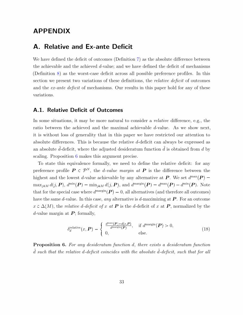
A. Relative and Ex-ante Deficit
We have defined the deficit of outcomes (Definition 7) as the absolute difference between
the achievable and the achieved d-value; and we have defined the deficit of mechanisms
(Definition 8) as the worst-case deficit across all possible preference profiles. In this
section we present two variations of these definitions, the relative deficit of outcomes
and the ex-ante deficit of mechanisms. Our results in this paper hold for any of these
variations.
A.1. Relative Deficit of Outcomes
In some situations, it may be more natural to consider a relative difference, e.g., the
ratio between the achieved and the maximal achievable d-value. As we show next,
it is without loss of generality that in this paper we have restricted our attention to
absolute differences. This is because the relative d-deficit can always be expressed as
an absolute d-deficit, where the adjusted desideratum function d is obtained from d by
scaling. Proposition 6 makes this argument precise.
To state this equivalence formally, we need to define the relative deficit: for any
preference profile P P PN , the d-value margin at P is the difference between the
highest and the lowest d-value achievable by any alternative at P . We set dmaxpP q �
maxjPM dpj,P q, dminpP q � minjPM dpj,P q, and dmarginpP q � dmaxpP q � dminpP q. Note
that for the special case where dmarginpP q � 0, all alternatives (and therefore all outcomes)
have the same d-value. In this case, any alternative is d-maximizing at P . For an outcome
x P ∆pMq, the relative d-deficit of x at P is the d-deficit of x at P , normalized by the
d-value margin at P ; formally,
δrelatived px,P q �
#dmaxpP q�dpx,P q
dmarginpP q, if dmarginpP q ¡ 0,
0, else.(18)
Proposition 6. For any desideratum function d, there exists a desideratum function
d such that the relative d-deficit coincides with the absolute d-deficit, such that for all
33
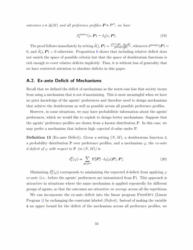
outcomes x P ∆pMq and all preference profiles P P PN , we have
δrelatived px,P q � δdpx,P q. (19)
The proof follows immediately by setting dpj,P q � dmaxpP q�dpj,P qdmarginpP q
, whenever dmarginpP q ¡
0, and dpj,P q � 0 otherwise. Proposition 6 shows that including relative deficit does
not enrich the space of possible criteria but that the space of desideratum functions is
rich enough to cover relative deficits implicitly. Thus, it is without loss of generality that
we have restricted attention to absolute deficits in this paper.
A.2. Ex-ante Deficit of Mechanisms
Recall that we defined the deficit of mechanisms as the worst-case loss that society incurs
from using a mechanism that is not d-maximizing. This is most meaningful when we have
no prior knowledge of the agents’ preferences and therefore need to design mechanisms
that achieve the desideratum as well as possible across all possible preference profiles.
However, in some situations, we may have probabilistic information about the agents’
preferences, which we would like to exploit to design better mechanisms. Suppose that
the agents’ preference profiles are drawn from a known distribution P. In this case, we
may prefer a mechanism that induces high expected d-value under P.
Definition 13 (Ex-ante Deficit). Given a setting pN,Mq, a desideratum function d,
a probability distribution P over preference profiles, and a mechanism ϕ, the ex-ante
d-deficit of ϕ with respect to P (in pN,Mq) is
δPd pϕq �¸
P PPNPrP s � δdpϕpP q,P q. (20)
Minimizing δPd pϕq corresponds to minimizing the expected d-deficit from applying ϕ
ex-ante (i.e., before the agents’ preferences are instantiated from P). This approach is
attractive in situations where the same mechanism is applied repeatedly for different
groups of agents, so that the outcomes are attractive on average across all the repetitions.
We can incorporate the ex-ante deficit into the linear program FindOpt (Linear
Program 1) by exchanging the constraint labeled (Deficit). Instead of making the variable
d an upper bound for the deficit of the mechanism across all preference profiles, we
34
need to make d an upper bound for the expected deficit of the mechanism, where this
expectation is taken with respect to the distribution P over preference profiles. We
achieve this by including the following constraint.
d ¥¸
P PPNPrP s �
�maxjPM
dpj,P q �¸jPM
fjpPq � dpj,P q
�. (Ex-ante deficit)
B. Strict Improvements from Hybrids in Theorem 2
Theorem 2 showed two weak inequalities for hybrid mechanisms. We now give an
example that shows that a hybrid of two mechanisms can in fact have a strictly lower
manipulability and a strictly lower deficit than both of its component mechanisms.
Example 3. Consider a problem with one agent and three alternatives a, b, c, where δ is
the worst-case deficit that arises from Plurality scoring. Let ϕ and ψ be two mechanisms
whose outcomes depend only on the agent’s relative ranking of b and c.
ϕ ψ
Report a b c a b c
If P : b © c 0 2/3 1/3 5/9 1/9 1/3
If P : c ¡ b 1/3 1/3 1/3 1/9 5/9 1/3
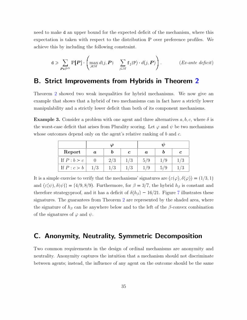
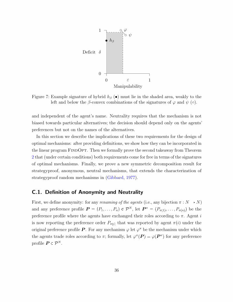
It is a simple exercise to verify that the mechanisms’ signatures are pεpϕq, δpϕqq � p1{3, 1q
and pεpψq, δpψqq � p4{9, 8{9q. Furthermore, for β � 3{7, the hybrid hβ is constant and
therefore strategyproof, and it has a deficit of δphβq � 16{21. Figure 7 illustrates these
signatures. The guarantees from Theorem 2 are represented by the shaded area, where
the signature of hβ can lie anywhere below and to the left of the β-convex combination
of the signatures of ϕ and ψ.
C. Anonymity, Neutrality, Symmetric Decomposition
Two common requirements in the design of ordinal mechanisms are anonymity and
neutrality. Anonymity captures the intuition that a mechanism should not discriminate
between agents; instead, the influence of any agent on the outcome should be the same
35
1
10
0
Manipulability
ε
Deficit δ
ϕψ
hβ
Figure 7: Example signature of hybrid hβ (•) must lie in the shaded area, weakly to theleft and below the β-convex combinations of the signatures of ϕ and ψ (�).
and independent of the agent’s name. Neutrality requires that the mechanism is not
biased towards particular alternatives; the decision should depend only on the agents’
preferences but not on the names of the alternatives.
In this section we describe the implications of these two requirements for the design of
optimal mechanisms: after providing definitions, we show how they can be incorporated in
the linear program FindOpt. Then we formally prove the second takeaway from Theorem
2 that (under certain conditions) both requirements come for free in terms of the signatures
of optimal mechanisms. Finally, we prove a new symmetric decomposition result for
strategyproof, anonymous, neutral mechanisms, that extends the characterization of
strategyproof random mechanisms in (Gibbard, 1977).
C.1. Definition of Anonymity and Neutrality
First, we define anonymity: for any renaming of the agents (i.e., any bijection π : N Ñ N)
and any preference profile P � pP1, . . . , Pnq P PN , let P π � pPπp1q, . . . , Pπpnqq be the
preference profile where the agents have exchanged their roles according to π. Agent i
is now reporting the preference order Pπpiq that was reported by agent πpiq under the
original preference profile P . For any mechanism ϕ let ϕπ be the mechanism under which
the agents trade roles according to π; formally, let ϕπpP q � ϕpP πq for any preference
profile P P PN .
36
Definition 14 (Anonymity). • A desideratum function d is anonymous if for all
renamings π : N Ñ N , preference profiles P P PN , and alternatives j P M , we
have dpj,P q � dpj,P πq (i.e., the d-value is independent of the order in which the
agents submit their preferences).
• A probability distribution P over preference profiles is anonymous if for all renam-
ings π : N Ñ N and preference profiles P P PN , we have PrP s � PrP πs (i.e.,
the probability of a preference profile does not depend on the order in which the
different preference orders appear).
• The worst-case deficit δd is anonymous if the underlying desideratum function d is
anonymous. The ex-ante deficit δPd is anonymous if the underlying desideratum
function and the probability distribution P are anonymous.
• A mechanism ϕ is anonymous if for all renamings π : N Ñ N and preference
profiles P P PN , we have ϕpP q � ϕπpP q (i.e., the outcome of the mechanism is
independent of the order in which the agents submit their preferences).
Next, we define neutrality: for any renaming of the alternatives (i.e., any bijection
$ : M Ñ M) and any preference order Pi P P, let P$i be the preference order under
which P$i : $pjq © $pj1q whenever Pi : j © j1 for any alternatives j, j1 PM . This means
that P$i corresponds to Pi, except that the all alternatives have been renamed according
to $. For any preference profile P � pP1, . . . , Pnq P PN , let P$ � pP$1 , . . . , P
$n q be the
preference profile where the alternatives inside the agents’ preference orders have been
renamed according to $. For any mechanism ϕ let ϕ$ be the mechanism under which
the alternatives are renamed according to $; formally, let ϕ$j pP q � ϕ$pjqpP$q for all
preference profile P P PN and alternative j PM .
Definition 15 (Neutrality). We define the following:
• A desideratum function d is neutral if for all renamings $ : M ÑM , preference
profiles P P PN , and alternatives j PM , we have dpj,P q � dp$pjq,P$q (i.e., the
d-value of any alternative is independent of its name).
• A probability distribution P over preference profiles is neutral if for all renamings
$ : M Ñ M and preference profiles P P PN , we have PrP s � PrP$s (i.e., the
probability of a preference profile does not depend on the names of the alternatives).
37

• The worst-case deficit δd is neutral if the underlying desideratum function d is
neutral. The ex-ante deficit δPd is neutral if the underlying desideratum function
and the probability distribution P are neutral.
• A mechanism ϕ is neutral if for all renamings $ : M Ñ M , preference profiles
P P PN , and alternatives j PM , we have ϕjpP q � ϕ$j pP q � ϕ$pjqpP$q (i.e., the
outcomes of the mechanism are independent of the names of the alternatives).
Incorporating anonymity and neutrality as additional constraints in the linear program
FindOpt is straightforward and can be done as follows.
Linear Program 1 (FindOpt), extended.
. . .
fjpPq � fjpPπq, @P P PN , j PM,π : N Ñ N bijection (Anonymity)
fjpPq � f$pjqpP$q, @P P PN , j PM,$ : M ÑM bijection (Neutrality)
C.2. Costlessness of Requiring Anonymity and Neutrality
With these notions of anonymity and neutrality in mind, observe that for any given
mechanism it is possible to construct an anonymous mechanism or a neutral mechanism
by randomizing over the roles of the agents or the roles of the alternatives in the
mechanism, respectively: let
ϕanonj pP q �
1
n!
¸π : N Ñ N
bijection
ϕπj pP q (21)
and
ϕneutj pP q �
1
m!
¸$ : M ÑM
bijection
ϕ$j pP q (22)
for all preference profiles P P PN and alternatives j PM . Observe that ϕanon and ϕneut
are simply hybrid mechanisms with many components, where each component is used
38
with a probability of 1n!
or 1m!
, respectively. With these definitions we can formally derive
the second main takeaway from Theorem 2.
Corollary 3. Given a problem pN,M, δq, where the deficit is anonymous/neutral/both,
for any mechanism ϕ there exists a mechanism ϕ that is anonymous/neutral/both and
has a weakly better signature than ϕ; formally, εpϕq ¤ εpϕq and δpϕq ¤ δpϕq
Proof. Observe that if the deficit δ is anonymous, then ϕ and ϕπ have the same signature
for any renaming of the agents π : N Ñ N . Consequently, ϕanon is a hybrid of n!
mechanisms which all have the same signature, and therefore it has a weakly better
signature by Theorem 2. Similarly, if δ is neutral, then ϕ and ϕ$ have the same signature
for any renaming of the alternatives $ : M ÑM , and the result follows analogously.
Intuitively, Corollary 3 means that, given the right desideratum, the two requirements
anonymity and neutrality are “free” in terms of manipulability and deficit. We do not
have to accept a less attractive signatures in order to achieve either property.
C.3. Non-trivial Signature Cost of Other Desiderata
In contrast to anonymity and neutrality, other common desiderata do not come for free,
such as Condorcet consistency, Pareto optimality, or even the rather weak requirement
of unanimity.
Definition 16 (Unanimity, Pareto Optimality, Condorcet Consistency). For a given
preference profile P P PN , define the following:
• An alternative j P M is a unanimity winner at P if for all agents i P N and all
other alternatives j1 P M we have Pi : j © j1. Let MunanpP q be the set of all
unanimity winners at P and M unanpP q �MzMunanpP q the set of non-winners.
• An alternative j P M Pareto dominates another alternative j1 P M at P if for
all agents i P N we have Pi : j © j1 and for some agent i1 we have Pi1 : j ¡
j1. j is Pareto optimal at P if there exists no other alternative j1 that Pareto
dominates j. Let MParetopP q be the set of Pareto optimal alternatives at P , and let
M ParetopP q �MzMParetopP q be the set of alternatives that are Pareto dominated
by another alternative at P .
39
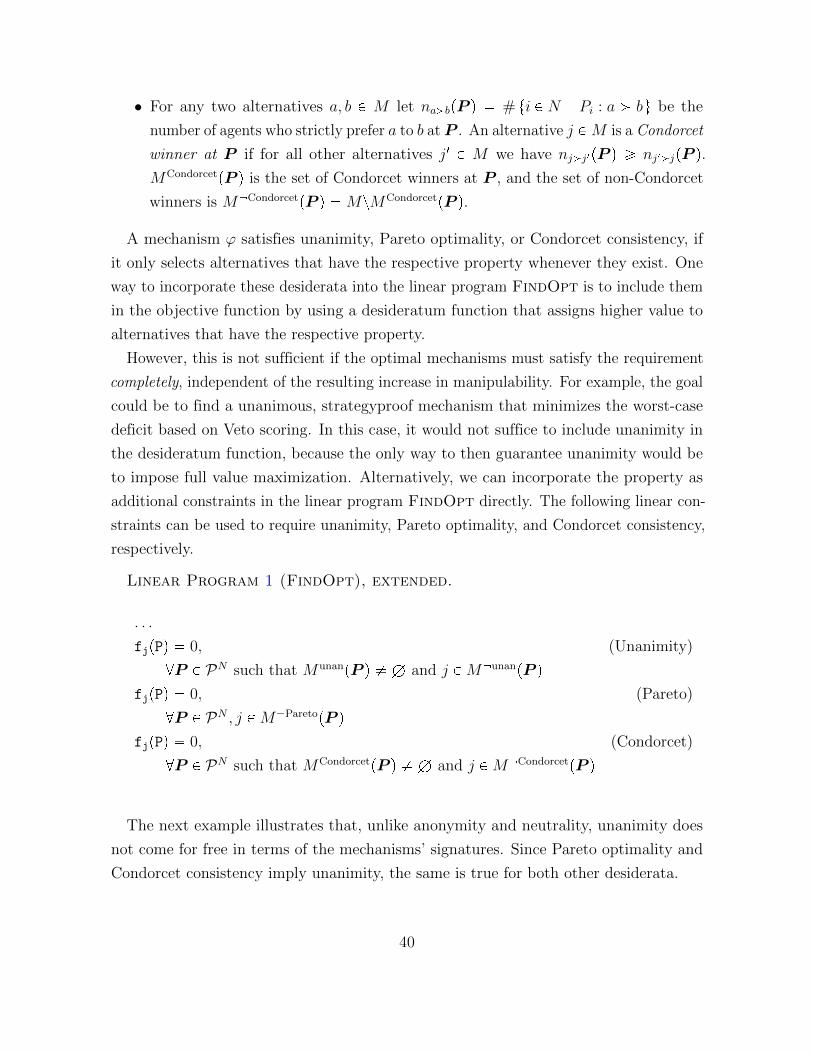
• For any two alternatives a, b P M let na¡bpP q � # ti P N | Pi : a ¡ bu be the
number of agents who strictly prefer a to b at P . An alternative j PM is a Condorcet
winner at P if for all other alternatives j1 P M we have nj¡j1pP q ¥ nj1¡jpP q.
MCondorcetpP q is the set of Condorcet winners at P , and the set of non-Condorcet
winners is M CondorcetpP q �MzMCondorcetpP q.
A mechanism ϕ satisfies unanimity, Pareto optimality, or Condorcet consistency, if
it only selects alternatives that have the respective property whenever they exist. One
way to incorporate these desiderata into the linear program FindOpt is to include them
in the objective function by using a desideratum function that assigns higher value to
alternatives that have the respective property.
However, this is not sufficient if the optimal mechanisms must satisfy the requirement
completely, independent of the resulting increase in manipulability. For example, the goal
could be to find a unanimous, strategyproof mechanism that minimizes the worst-case
deficit based on Veto scoring. In this case, it would not suffice to include unanimity in
the desideratum function, because the only way to then guarantee unanimity would be
to impose full value maximization. Alternatively, we can incorporate the property as
additional constraints in the linear program FindOpt directly. The following linear con-
straints can be used to require unanimity, Pareto optimality, and Condorcet consistency,
respectively.
Linear Program 1 (FindOpt), extended.
. . .
fjpPq � 0, (Unanimity)
@P P PN such that MunanpP q � H and j PM unanpP q
fjpPq � 0, (Pareto)
@P P PN , j PM ParetopP q
fjpPq � 0, (Condorcet)
@P P PN such that MCondorcetpP q � H and j PM CondorcetpP q
The next example illustrates that, unlike anonymity and neutrality, unanimity does
not come for free in terms of the mechanisms’ signatures. Since Pareto optimality and
Condorcet consistency imply unanimity, the same is true for both other desiderata.
40
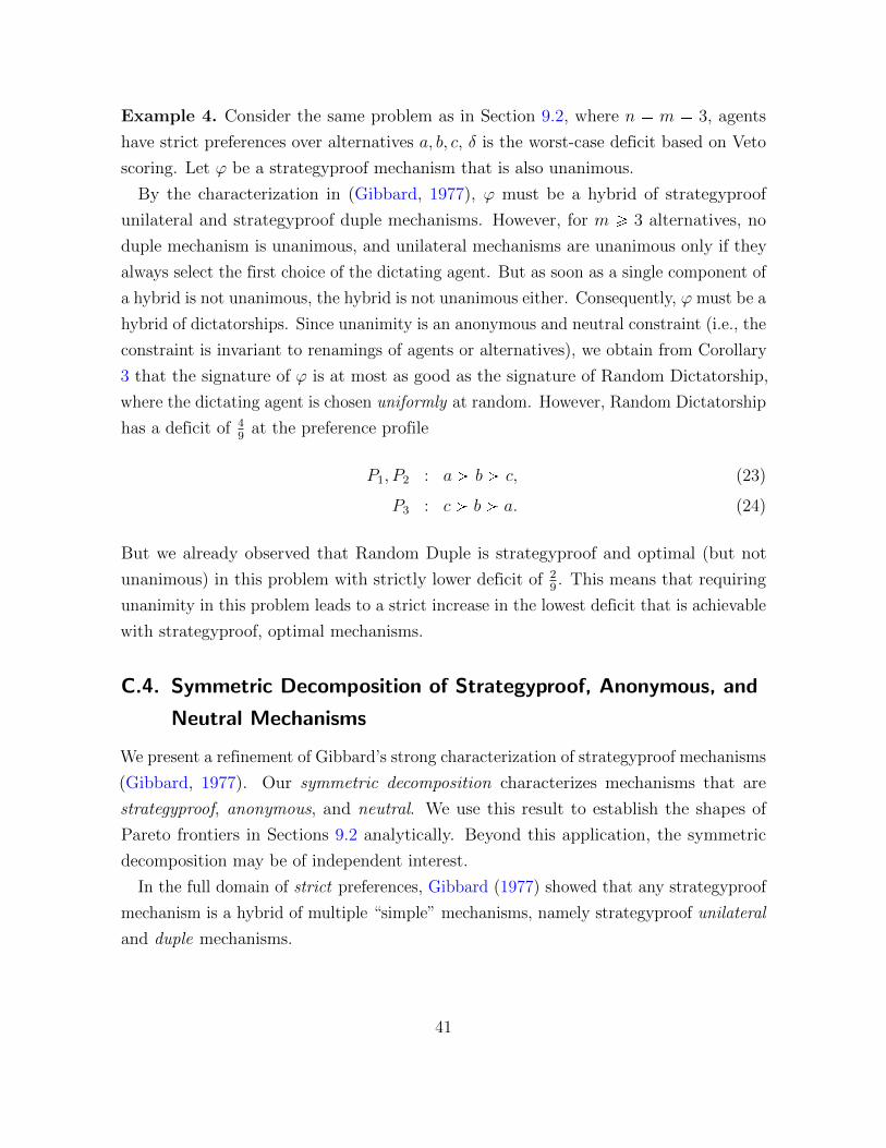
Example 4. Consider the same problem as in Section 9.2, where n � m � 3, agents
have strict preferences over alternatives a, b, c, δ is the worst-case deficit based on Veto
scoring. Let ϕ be a strategyproof mechanism that is also unanimous.
By the characterization in (Gibbard, 1977), ϕ must be a hybrid of strategyproof
unilateral and strategyproof duple mechanisms. However, for m ¥ 3 alternatives, no
duple mechanism is unanimous, and unilateral mechanisms are unanimous only if they
always select the first choice of the dictating agent. But as soon as a single component of
a hybrid is not unanimous, the hybrid is not unanimous either. Consequently, ϕ must be a
hybrid of dictatorships. Since unanimity is an anonymous and neutral constraint (i.e., the
constraint is invariant to renamings of agents or alternatives), we obtain from Corollary
3 that the signature of ϕ is at most as good as the signature of Random Dictatorship,
where the dictating agent is chosen uniformly at random. However, Random Dictatorship
has a deficit of 49
at the preference profile
P1, P2 : a ¡ b ¡ c, (23)
P3 : c ¡ b ¡ a. (24)
But we already observed that Random Duple is strategyproof and optimal (but not
unanimous) in this problem with strictly lower deficit of 29. This means that requiring
unanimity in this problem leads to a strict increase in the lowest deficit that is achievable
with strategyproof, optimal mechanisms.
C.4. Symmetric Decomposition of Strategyproof, Anonymous, and
Neutral Mechanisms
We present a refinement of Gibbard’s strong characterization of strategyproof mechanisms
(Gibbard, 1977). Our symmetric decomposition characterizes mechanisms that are
strategyproof, anonymous, and neutral. We use this result to establish the shapes of
Pareto frontiers in Sections 9.2 analytically. Beyond this application, the symmetric
decomposition may be of independent interest.
In the full domain of strict preferences, Gibbard (1977) showed that any strategyproof
mechanism is a hybrid of multiple “simple” mechanisms, namely strategyproof unilateral
and duple mechanisms.
41
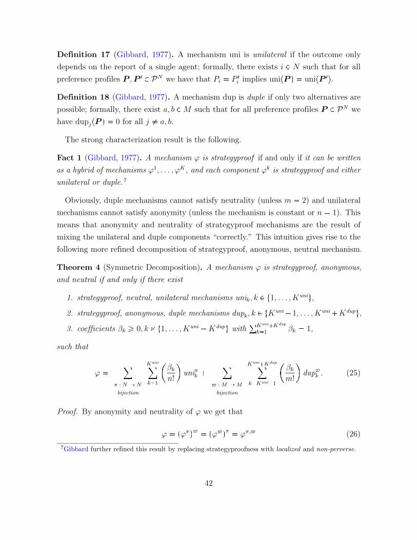
Definition 17 (Gibbard, 1977). A mechanism uni is unilateral if the outcome only
depends on the report of a single agent; formally, there exists i P N such that for all
preference profiles P ,P 1 P PN we have that Pi � P 1i implies unipP q � unipP 1q.
Definition 18 (Gibbard, 1977). A mechanism dup is duple if only two alternatives are
possible; formally, there exist a, b PM such that for all preference profiles P P PN we
have dupjpP q � 0 for all j � a, b.
The strong characterization result is the following.
Fact 1 (Gibbard, 1977). A mechanism ϕ is strategyproof if and only if it can be written
as a hybrid of mechanisms ϕ1, . . . , ϕK , and each component ϕk is strategyproof and either
unilateral or duple.7
Obviously, duple mechanisms cannot satisfy neutrality (unless m � 2) and unilateral
mechanisms cannot satisfy anonymity (unless the mechanism is constant or n � 1). This
means that anonymity and neutrality of strategyproof mechanisms are the result of
mixing the unilateral and duple components “correctly.” This intuition gives rise to the
following more refined decomposition of strategyproof, anonymous, neutral mechanism.
Theorem 4 (Symmetric Decomposition). A mechanism ϕ is strategyproof, anonymous,
and neutral if and only if there exist
1. strategyproof, neutral, unilateral mechanisms unik, k P t1, . . . , Kuniu,
2. strategyproof, anonymous, duple mechanisms dupk, k P tKuni� 1, . . . , Kuni�Kdupu,
3. coefficients βk ¥ 0, k P t1, . . . , Kuni �Kdupu with°Kuni�Kdup
k�1 βk � 1,
such that
ϕ �¸
π : N Ñ N
bijection
Kuni¸k�1
�βkn!
uniπk �
¸$ : M ÑM
bijection
Kuni�Kdup¸k�Kuni�1
�βkm!
dup$k . (25)
Proof. By anonymity and neutrality of ϕ we get that
ϕ � pϕπq$ � pϕ$qπ � ϕπ,$ (26)
7Gibbard further refined this result by replacing strategyproofness with localized and non-perverse.
42
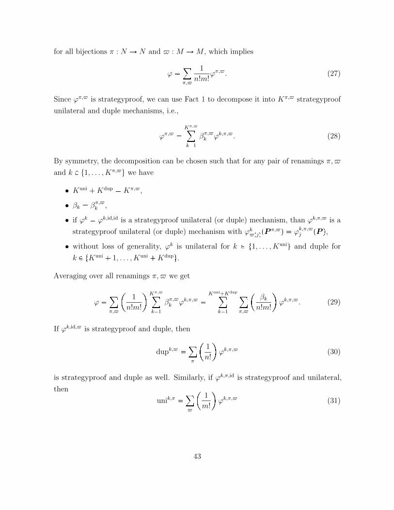
for all bijections π : N Ñ N and $ : M ÑM , which implies
ϕ �¸π,$
1
n!m!ϕπ,$. (27)
Since ϕπ,$ is strategyproof, we can use Fact 1 to decompose it into Kπ,$ strategyproof
unilateral and duple mechanisms, i.e.,
ϕπ,$ �Kπ,$¸k�1
βπ,$k ϕk,π,$. (28)
By symmetry, the decomposition can be chosen such that for any pair of renamings π,$
and k P t1, . . . , Kπ,$u we have
• Kuni �Kdup � Kπ,$,
• βk � βπ,$k ,
• if ϕk � ϕk,id,id is a strategyproof unilateral (or duple) mechanism, than ϕk,π,$ is a
strategyproof unilateral (or duple) mechanism with ϕk$pjqpPπ,$q � ϕk,π,$j pP q,
• without loss of generality, ϕk is unilateral for k P t1, . . . , Kuniu and duple for
k P tKuni � 1, . . . , Kuni �Kdupu.
Averaging over all renamings π,$ we get
ϕ �¸π,$
�1
n!m!
Kπ,$¸k�1
βπ,$k ϕk,π,$ �Kuni�Kdup¸
k�1
¸π,$
�βkn!m!
ϕk,π,$. (29)
If ϕk,id,$ is strategyproof and duple, then
dupk,$ �¸π
�1
n!
ϕk,π,$ (30)
is strategyproof and duple as well. Similarly, if ϕk,π,id is strategyproof and unilateral,
then
unik,π �¸$
�1
m!
ϕk,π,$ (31)
43
is strategyproof and unilateral as well. With this we can rewrite (29) as
ϕ �Kuni¸k�1
¸π
βkn!
unik,π �Kuni�Kdup¸k�Kuni�1
¸$
βkm!
dupk,$, (32)
which is precisely the symmetric decomposition (25).
The symmetric decomposition (25) is a consequence of Gibbard’s strong characteriza-
tion and the fact that for any anonymous, neutral mechanism we have ϕ � ϕπ,$. It is
symmetric in the sense that for any component unik (or dupk) that occur with coefficient
βk, the corresponding component unik,π (or dupk,$) occur with the same coefficient.
(25) decomposes ϕ into two parts: a neutral part on the left, that gets “anonymized”
by randomization, and an anonymous part on the right that gets “neutralized” by
randomization.
C.5. Connection to Gibbard’s Strong Characterization of
Strategyproof Random Mechanisms
In Section 9.2 we have studied the Pareto frontier for two different desiderata, namely
Plurality and Veto scoring. Juxtaposing the two examples shows an interesting connection
to earlier work that characterized strategyproof random mechanisms: Gibbard (1977)
showed that in a domain with three or more alternatives and strict preferences, any
mechanism that is strategyproof must be a probability mixture (i.e., a hybrid with an
arbitrary number of components) of strategyproof unilateral mechanisms (i.e., whose
random outcomes depend only on the preference order of a single agent) and strategyproof
duple mechanisms (i.e., which assign positive probability to at most two alternatives).
Our examples show that the optimal strategyproof mechanisms for the particular
problems are exactly the two extremes of this representation: when the desideratum is
based on Plurality scoring, optimal strategyproof mechanism arise by randomizing over
unilateral mechanisms only, namely dictatorships. Conversely, when the desideratum
is based on Veto scoring, optimal strategyproof mechanisms arise by randomizing over
duple mechanisms only, namely the majority vote between two alternatives. Thus, our
two examples teach us in what sense unilateral and duple mechanisms can be understood
to reside on “opposite ends” of the spectrum of strategyproof mechanisms.
44
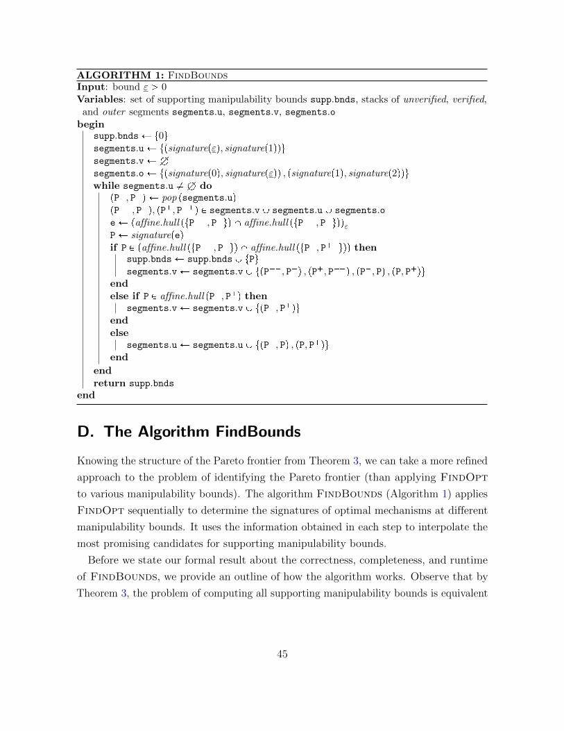
ALGORITHM 1: FindBoundsInput: bound ε ¡ 0Variables: set of supporting manipulability bounds supp.bnds, stacks of unverified, verified,and outer segments segments.u, segments.v, segments.o
beginsupp.bndsÐ t0usegments.uÐ tpsignaturepεq, signaturep1qqusegments.vÐHsegments.oÐ tpsignaturep0q, signaturepεqq , psignaturep1q, signaturep2qquwhile segments.u � H do
pP�, P�q Ð pop psegments.uqpP��, P�q, pP�, P��q P segments.vY segments.uY segments.oeÐ paffine.hull ptP��, P�uq X affine.hull ptP��, P�uqqεPÐ signaturepeqif P P paffine.hull ptP��, P�uq X affine.hull ptP�, P��uqq then
supp.bndsРsupp.bndsY tPusegments.vРsegments.vY tpP��, P�q , pP�, P��q , pP�, Pq , pP, P�qu
endelse if P P affine.hull pP�, P�q then
segments.vÐ segments.vY tpP�, P�quendelse
segments.uÐ segments.uY tpP�, Pq , pP, P�quend
endreturn supp.bnds
end
D. The Algorithm FindBounds
Knowing the structure of the Pareto frontier from Theorem 3, we can take a more refined
approach to the problem of identifying the Pareto frontier (than applying FindOpt
to various manipulability bounds). The algorithm FindBounds (Algorithm 1) applies
FindOpt sequentially to determine the signatures of optimal mechanisms at different
manipulability bounds. It uses the information obtained in each step to interpolate the
most promising candidates for supporting manipulability bounds.
Before we state our formal result about the correctness, completeness, and runtime
of FindBounds, we provide an outline of how the algorithm works. Observe that by
Theorem 3, the problem of computing all supporting manipulability bounds is equivalent
45
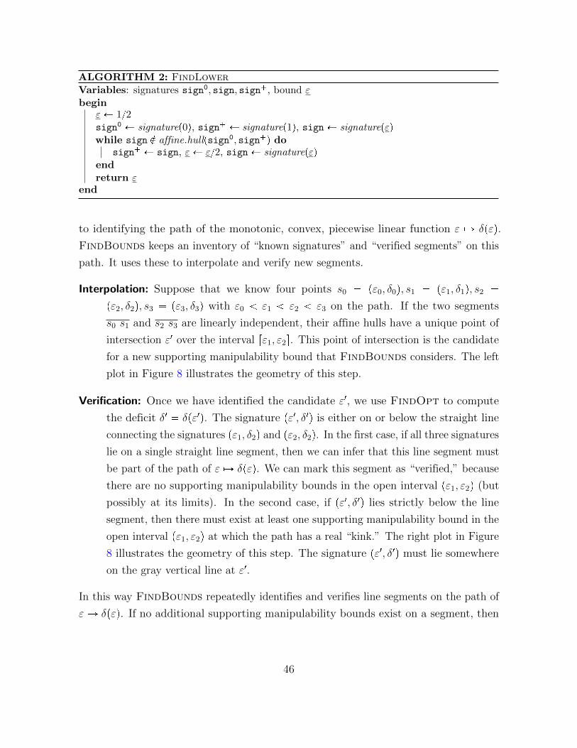
ALGORITHM 2: FindLowerVariables: signatures sign0, sign, sign�, bound εbegin
εÐ 1{2sign0 Ð signaturep0q, sign� Ð signaturep1q, signÐ signaturepεqwhile sign R affine.hullpsign0, sign�q do
sign� Ð sign, εÐ ε{2, signÐ signaturepεqendreturn ε
end
to identifying the path of the monotonic, convex, piecewise linear function ε ÞÑ δpεq.
FindBounds keeps an inventory of “known signatures” and “verified segments” on this
path. It uses these to interpolate and verify new segments.
Interpolation: Suppose that we know four points s0 � pε0, δ0q, s1 � pε1, δ1q, s2 �
pε2, δ2q, s3 � pε3, δ3q with ε0 ε1 ε2 ε3 on the path. If the two segments
s0 s1 and s2 s3 are linearly independent, their affine hulls have a unique point of
intersection ε1 over the interval rε1, ε2s. This point of intersection is the candidate
for a new supporting manipulability bound that FindBounds considers. The left
plot in Figure 8 illustrates the geometry of this step.
Verification: Once we have identified the candidate ε1, we use FindOpt to compute
the deficit δ1 � δpε1q. The signature pε1, δ1q is either on or below the straight line
connecting the signatures pε1, δ2q and pε2, δ2q. In the first case, if all three signatures
lie on a single straight line segment, then we can infer that this line segment must
be part of the path of ε ÞÑ δpεq. We can mark this segment as “verified,” because
there are no supporting manipulability bounds in the open interval pε1, ε2q (but
possibly at its limits). In the second case, if pε1, δ1q lies strictly below the line
segment, then there must exist at least one supporting manipulability bound in the
open interval pε1, ε2q at which the path has a real “kink.” The right plot in Figure
8 illustrates the geometry of this step. The signature pε1, δ1q must lie somewhere
on the gray vertical line at ε1.
In this way FindBounds repeatedly identifies and verifies line segments on the path of
ε ÞÑ δpεq. If no additional supporting manipulability bounds exist on a segment, then
46
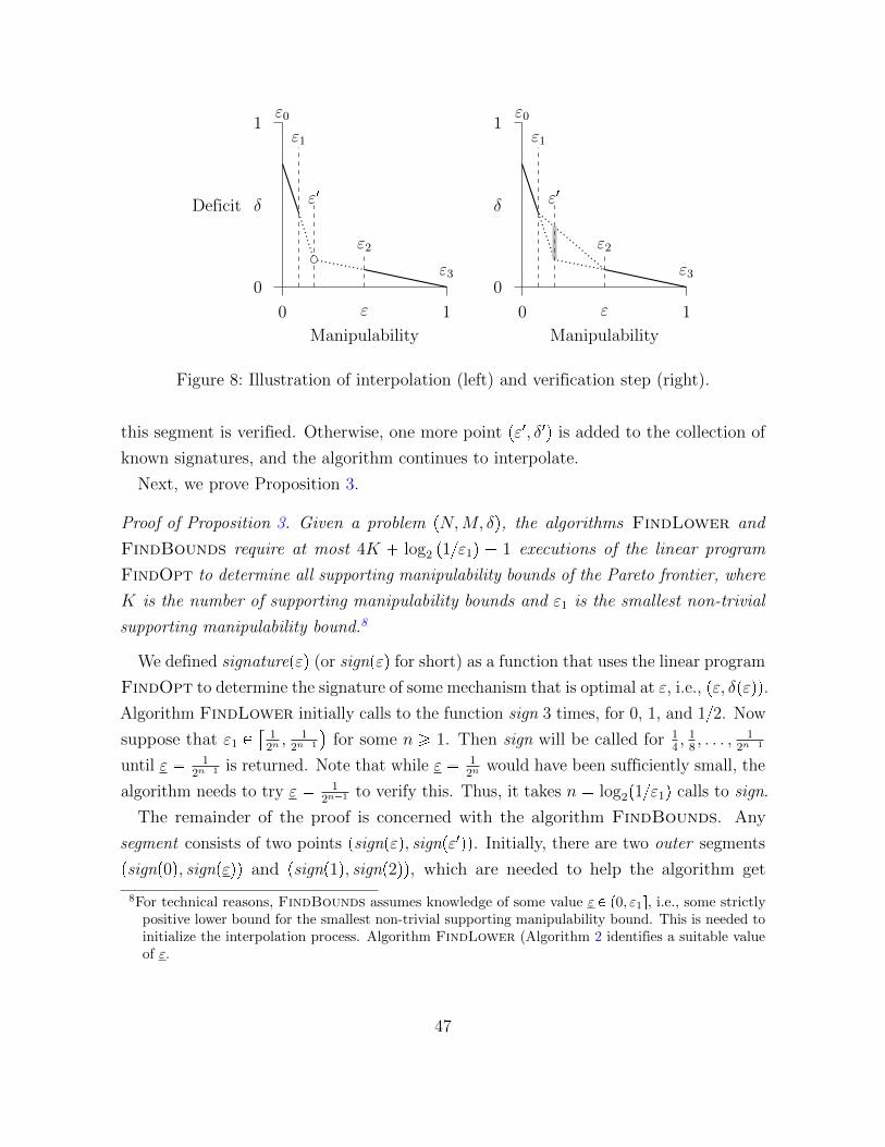
1
10
0
Manipulability
ε
Deficit δ ε1
ε1
ε2
ε0
ε3
1
10
0
Manipulability
ε
δ ε1
ε1
ε2
ε0
ε3
Figure 8: Illustration of interpolation (left) and verification step (right).
this segment is verified. Otherwise, one more point pε1, δ1q is added to the collection of
known signatures, and the algorithm continues to interpolate.
Next, we prove Proposition 3.
Proof of Proposition 3. Given a problem pN,M, δq, the algorithms FindLower and
FindBounds require at most 4K � log2 p1{ε1q � 1 executions of the linear program
FindOpt to determine all supporting manipulability bounds of the Pareto frontier, where
K is the number of supporting manipulability bounds and ε1 is the smallest non-trivial
supporting manipulability bound.8
We defined signaturepεq (or signpεq for short) as a function that uses the linear program
FindOpt to determine the signature of some mechanism that is optimal at ε, i.e., pε, δpεqq.
Algorithm FindLower initially calls to the function sign 3 times, for 0, 1, and 1{2. Now
suppose that ε1 P�
12n, 1
2n�1
�for some n ¥ 1. Then sign will be called for 1
4, 1
8, . . . , 1
2n�1
until ε � 12n�1 is returned. Note that while ε � 1
2nwould have been sufficiently small, the
algorithm needs to try ε � 12n�1 to verify this. Thus, it takes n � log2p1{ε1q calls to sign.
The remainder of the proof is concerned with the algorithm FindBounds. Any
segment consists of two points psignpεq, signpε1qq. Initially, there are two outer segments
psignp0q, signpεqq and psignp1q, signp2qq, which are needed to help the algorithm get
8For technical reasons, FindBounds assumes knowledge of some value ε P p0, ε1s, i.e., some strictlypositive lower bound for the smallest non-trivial supporting manipulability bound. This is needed toinitialize the interpolation process. Algorithm FindLower (Algorithm 2 identifies a suitable valueof ε.
47
started. The algorithm maintains a decomposition of the interval rε, 1s, which initially
consists of a single unverified segment. In every execution of the while-loop, Find-
Bounds selects an unverified segment psignpε�q, signpε�qq. Then it uses the segments to
the left and right psignpε��q, signpε�qq and psignpε�q, signpε��qq to “guess” the position
of a new supporting manipulability bound between ε� and ε�. This guess e is the ε-value
of the point of intersection of the affine hulls of the two segments, i.e.,
e ��affine.hull
� signpε��q, signpε�q
(�X affine.hull
� signpε�q, signpε��q
(��ε, (33)
where affine.hull denotes the affine hull. This value is unique and lies inside the open
interval pε�, ε�q (by Claim 1). Now P � signpeq is computed using the linear program
FindOpt, and one of three cases can occur:
1. P may be equal to the unique point of intersection
affine.hull� signpε��q, signpε�q
(�X affine.hull
� signpε�q, signpε��q
(�. (34)
In this case, e is a supporting manipulability bound. Furthermore, the segments
psignpε��q, signpε�qq, psignpε�q, Pq, pP, signpε�qq, and psignpε�q, signpε��qq. are
all part of the signature of the Pareto frontier (by Claim 3), and there are no
other supporting manipulability bound in the interval p�, �q. FindBounds
marks the four segments as verified and includes e in the collection of supporting
manipulability bounds.
2. P lies in the affine hull of the segment psignpε�q, signpε�qq. Then by Claim 2,
Conv� signpε�q, P
(�Y Conv
� P, signpε�q
(�(35)
is part of the signature of the Pareto frontier, and there are no supporting ma-
nipulability bounds inside the interval pε�, ε�q. FindBounds marks the segment
psignpε�q, signpε�qq as verified.
3. In any other case, FindBounds splits the segment psignpε�q, signpε�qq by creating
two new unverified segments
�signpε�q, P
�and
�P, signpε�q
�. (36)
48
We first show correctness of FindBounds, then completeness:
Correctness FindBounds stops running when there are no more unverified segments.
Assume towards contradiction that there exists a supporting manipulability bound
ε P pε, 1q that has not been identified. Then this supporting manipulability bound
lies in some segment rε�, ε�s that was verified.
If the verification happened in a case 1, Claim 3 ensures that there is no other
supporting manipulability bound, i.e., the supporting manipulability bound would
have been added to the collection during the analysis of the interval p�, �q.
If the verification happened in a case 2, Claim 2 ensures that ε R pε�, ε�q, so
that ε � ε� (without loss of generality we can assume ε � ε�, the case ε � ε�
is analogous). The segment psignpε��q, signpε�qq was not a verified segment at
this time, otherwise this would be a case 1. Thus, at some future step some
segment psignpεq, signpε�qq with a right end-point in signpε�q was verified. But
at this step signpε�q was on the intersection of the affine hulls of the segments�signp˜εq, signpεq
�and psignpε�q, signpε�qq. This creates a case 1, and thus ε was
identified as a supporting manipulability bound in this step.
Completeness It remains to be shown that FindBounds stops at some point. By Claim
4, for ever two adjacent supporting manipulability bounds εk, εk�1, FindBounds
computes at most three points signpε1q, signpε2q, signpε3q with ε1, ε2, ε3 P pεk, εk�1q.
Since there is a finite number of supporting manipulability bounds, FindBounds
loops at most 3� 1 � 4 times per interval, which establishes completeness. The
run-time bound follows by observing that there exist K � 2 intervals between the
smallest non-trivial bound ε1 and the largest bound ε. However, we may need to
check the interval pε, 1q if ε 1. Thus, using ε from FindLower we require at
most 4K � 4 executions of FindOpt to run FindBounds.
Claim 1. e P pε�, ε�q
Proof. By convexity of ε ÞÑ δpεq, we get that e P rε�, ε�s.
Now suppose that e � ε�. Then ε� P affine.hull ptsignpε�q, signpε��quq. Since ε�
ε�, the segments psignpε�q, signpε�qq and psignpε�q, signpε��qq would have been verified
in a previous step. But this is a contradiction to the assumption that psignpε�q, signpε�qq
was an unverified segment.
49
Claim 2. For 0 ¤ ε�1 ε0 ε1 ¤ 1, if
signpε0q P Conv ptsignpε�1q, signpε1quq , (37)
then
Conv ptsignpε�1q, signpε1quq (38)
is part of the signature of the Pareto frontier.
Proof. Assume towards contradiction that Conv ptsignpε�1q, signpε1quq is not part of the
signature of the Pareto frontier. Then by convexity of ε ÞÑ δpεq there exists γ P p0, 1q
with
δpϕp1�γqε�1�γε1q p1� γqδpϕε�1q � γδpϕε1q. (39)
If ε1 � p1� γqε�1 � γε1 ¡ ε0, then for γ1 � ε0�ε�1
ε1�ε�1we get
p1� γ1qδpϕε�1q � γ1δpϕε1q δpϕε0q � δpϕp1�γ1qε�1�γ1ε1q, (40)
a contradiction to convexity of ε ÞÑ δpεq. The argument for ε1 ε0 is analogous.
Claim 3. For 0 ¤ ε�2 ε�1 ε0 ε1 ε2 ¤ 1, if
tsignpεqu � affine.hull ptsignpε�2q, signpε�1quq X affine.hull ptsignpε1q, signpε2quq , (41)
then
Conv ptsignpε0q, signpε�2quq (42)
is part of the signature of the Pareto frontier.
Proof. The claim follows by applying Claim 2 twice.
Claim 4. For any two adjacent supporting manipulability bounds εk, εk�1, FindBounds
computes at most three points signpε1q, signpε2q, signpε3q with ε1, ε2, ε3 P pεk, εk�1q.
Proof. Suppose that signpε1q, signpε2q, and signpε3q are computed in this order. If
ε3 minpε1, ε2q, then ε1 must be a supporting manipulability bound by convexity
of ε ÞÑ δpεq, which is a contradiction. The same holds if ε3 ¡ maxpε1, ε2q. If ε3 P
50
pminpε1, ε2q,maxpε1, ε2qq, the segment
psignpminpε1, ε2qq, signpmaxpε1, ε2qqq (43)
is verified (case (2)). Another guess ε4 that lies within rεk, εk�1s involve the segment
psignpε1q, signpε2qq. Thus, by convexity of ε ÞÑ δpεq, ε4 is a supporting manipulability
bound.
This concludes the proof of Proposition 3
The interpolation process in FindBounds is set up in such a way that at most 4
executions of FindOpt are required for finding each supporting manipulability bound.
Thus, assuming that representatives of Optpεkq must be determined by executing
FindOpt at each εk, FindBounds is at most a constant factor 4 slower than an algorithm
that correctly “guesses” all supporting manipulability bounds and uses FindOpt for
these only.
E. Alternative Domains and Desiderata
With the exception of the examples in Sections 9.2, we have formulated our results for
the general domain with weak preferences. In the following Section E.1, we explain
how our findings continue to hold in many other interesting domains. Subsequently, in
Section E.2, we discuss the expressiveness of desideratum functions for the purpose of
encoding desiderata.
E.1. Domain Restrictions
We have proven our results (Theorems 1 through 3 and Proposition 2) for the unrestricted
preference domain with indifferences. However, all these results continue to hold when
the domain is restricted by only admitting a subset of the possible preference profiles.
Formally, let P � PN be any subset of the set of preference profiles; then all our results
still hold, even if we admit only preference profiles from P . This extension is possible
because none of our proofs make use of the richness of the full domain.
Important domains that can be expressed as domain restrictions P � PN are:
51
• The full domain of strict ordinal preferences, which is the basis for the classical
impossibility results pertaining to strategyproofness of deterministic mechanisms
(Gibbard, 1973; Satterthwaite, 1975) and random mechanisms (Gibbard, 1977).
• The assignment domain, where each agent must be assigned to a single, indivisible
object (e.g., a seat at a public school) (Abdulkadiroglu and Sonmez, 2003).
• The two-sided matching domain, where agents of two different types must be
matched to each other to form pairs (e.g., men and women, doctors and hospitals,
mentors and mentees), and variations of this domain, such as matching with couples
(Roth, 1984).
• The combinatorial assignment domain, where agents receive bundles of indivisible
objects (e.g., schedules with multiple courses) (Budish, 2011)
Of course, the fact that our results continue to hold in these domains does not mean that
the actual Pareto frontiers will be equal across the different domains. On the contrary,
one would expect optimal mechanisms to be highly adapted to the particular domain in
which they are designed to operate.
Remark 7 (Full Utility Assumption). One essential ingredient to our results is the fact
that ε-approximate strategyproofness can be equivalently expressed via a finite set of
linear constraints. Theorem 1, which yields this equivalence, relies on the assumption
of full utility : given a preference order Pi, the agent i can have vNM utility function
ui P UPi that represents this preference order (and is bounded between 0 and 1). A
domain restriction that excludes subsets of utility functions would violate this condition.
For example, suppose that we imposed the additional restriction that the agent’s utility
are normalized (i.e., }ui}2 �b°
jPM uipjq2 � 1). This restriction limits the gain that an
agent can possibly obtain from misreporting in a non-linear way. The linear constraints
from Theorem 1 would be sufficient for ε-approximate strategyproofness. However, they
would no longer be necessary, and we would lose equivalent.
E.2. Encoding Desiderata via Desideratum Functions
desideratum functions are a very versatile means to express different design goals that
the mechanism designer may have. We have already seen how they can be used to reflect
desiderata based on Plurality scoring (Example 1), Condorcet consistency (Examples
52
2), or Veto scoring (Section 9.2). We now give additional examples that illustrate how
desideratum functions can be used to encode common desiderata.
Binary Desiderata Many desirable properties of mechanisms are simply properties
of the alternatives they select at any given preference profile. For instance, Pareto
optimality requires the mechanism to choose alternatives that are not Pareto dominated
by any other alternative at the respective preference profile. In general, let Θ be a
desirable property that an alternative can have at some preference profile (e.g., Pareto
optimality). Desideratum functions can capture Θ by setting
dpj,P q �
#1, if alternative j has property Θ at P ,
0, else.(44)
The d-deficit of a mechanism at a given preference profile,
δdpϕpP q,P q � maxjPM
dpj,P q �¸jPM
ϕjpP q � dpj,P q, (45)
has a straightforward interpretation: it is simply the “probability that an alternative
selected by ϕ at P violates property Θ at P .” Consequently, if δ is the worst-case deficit,
then the probability that ϕ selects an alternative that violates Θ is at most δpϕq across
all preference profiles. Alternatively, if δP is the ex-ante deficit, then δPpϕq is the ex-ante
probability (i.e., before the preferences have been reported) that ϕ selects an alternative
that violates Θ, given the prior distribution P over agents’ preference profiles.
Common binary desiderata include
• unanimity : if all agents agree on a first choice, this alternative should be selected,
• Condorcet consistency : if some alternatives weakly dominate any other alternatives
in a pairwise majority comparison, one of these alternatives should be selected,
• Pareto optimality : only undominated alternatives should be selected,
• egalitarian fairness: let Rpjq � maxiPN rankPipjq be the rank of alternative j in
the preference order of the agent who likes it least, then only alternatives with
minimal Rpjq should be selected.
While not all of these desiderata are in conflict with strategyproofness individually,
53
their combinations may be. It is possible to encode combinations of binary properties:
given two desideratum functions d1 and d2, the minimum d � minpd1, d2q is again a
desideratum function, and it expresses the desideratum that both properties (encoded
by d1 and d2) should hold simultaneously; and the maximum d � maxpd1, d2q expresses
that at least one of the properties should hold.
Even in the absence of a clear-cut objective, a desideratum may be implicitly specified
via a target mechanism. A target mechanism φ is a mechanism that one would like
to use if there were no concerns about manipulability (Birrell and Pass, 2011). The
desideratum function induced by φ takes value 1 at the alternatives that are selected by
φ at the respective preference profiles, or equivalently, dpj,P q � φjpP q. An analogous
construction is possible for a target correspondence Φ, which is a mechanism that selects
a set of alternatives. To reflect a target correspondence, the desideratum function can be
chosen as dpj,P q � 1 if j P ΦpP q and dpj,P q � 0 otherwise, where we denote by ΦpP q
the set of alternatives selected by the correspondence Φ at P .
In the assignment domain, our notion of Pareto optimality turns into ex-post effi-
ciency, which is an important baseline requirement for many assignment mechanisms.
Featherstone (2011) introduced v-rank efficiency, which is a refinement of ex-post effi-
ciency (and implies ordinal efficiency). He showed that for any rank valuation v, the
set of v-rank efficient assignments is equal to the convex hull of the set of deterministic
v-rank efficient assignments. Thus, v-rank efficiency is representable by a desideratum
function by setting dpa,P q � 1 for all alternatives a that correspond to a v-rank efficient
deterministic assignment. In two-sided matching, it is often important to select stable
matchings to prevent blocking pairs from matching outside the mechanism and thereby
causing unraveling of the market. Since stability is a property of deterministic matchings,
we can encode this desideratum by a desideratum function.
With any such desideratum function in hand, we can then define a notion of deficit
and use the results in this paper to understand the respective Pareto frontier.
Remark 8 (Linearity Assumption). One example of a desideratum that cannot be
represented by a desideratum function is the intermediate efficiency requirement of
ordinal efficiency for assignment mechanisms. To see this, note that ordinal efficiency
coincides with ex-post efficiency on deterministic assignments. However, the convex
combination of two ordinally efficient assignments is not necessarily again ordinally
efficient. In general, to be able to encode a desideratum via a desideratum function, the
54
societal value of any random outcome x must depend in a linear fashion on the societal
value of the individual alternatives (see Definition 5). Ordinal efficiency violates this
requirement.
Quantifiable Desiderata In some situations, there exists a quantified notion of the
desirability of different alternatives at different preference profiles. Straightforward
examples are desiderata based on positional scoring. Formally, a scoring function
v : t1, . . . ,mu Ñ R is a mapping that associates a score vprq with selecting some agent’s
rth choice alternative. Typical examples include Borda (i.e., vprq � m � r for all
r P t1, . . . ,mu), Plurality (i.e., vp1q � 1 and vprq � 0 for r � 1), and Veto (i.e., vprq � 0
for all r � m and vpmq � �1). The score of an alternative at a preference profile is
then determined by summing the scores of this alternative under the different preference
orders of the agents. Formally,
scvpj,P q �¸iPN
vprankPipjqq, (46)
where rankPipjq is the rank of alternative j in preference order Pi. For any scoring-based
desideratum, the respective desideratum function arises by scaling scv as follows:
dpj,P q �
#scvpj,P q�minj1PM scvpj1,P q
maxj1PM scvpj1,P q�minj1PM scvpj1,P q, if maxj1PM scvpj
1,P q ¡ minj1PM scvpj1,P q
0, else.
In the assignment domain, the rank valuation v is used to determine the v-rank value
of any assignment. This induces a scoring function on the corresponding alternatives.
Consequently, instead of viewing v-rank efficiency as a binary desideratum, the quantified
desideratum could be to maximize the v-rank value. This natural measure of societal
value was put forward by Featherstone (2011).
In quasi-linear domains, a common objective is to maximize the sum of the agents’
cardinal utilities. For situations where this aggregate value is interesting, Procaccia and
Rosenschein (2006) proposed to maximize a conservative estimate of this value instead.
This (slightly unorthodox) desideratum is also representable by a desideratum function.
Even though the vNM utilities in our model do not have to be comparable across agents,
one may choose to maximize the sum of these utilities. However, since agents only report
55
ordinal preferences, we cannot maximize their utilities directly. Instead, we can maximize
a conservative estimate for this sum. Formally, the respective desideratum would be to
maximize
dpj,P q � infu1PUP1 ,...,unPUPn
¸iPN
uipjq. (47)
Recall that we bounded utilities between 0 and 1, and let us assume that maxjPM uipjq � 1.
Then the aggregate utility from any outcome x P ∆pMq is lowest if agents have utility
(close to) 0 for all except their first choices. Thus, maximizing the conservative lower
bound for aggregate utility in our model corresponds to selecting an alternative that
is the first choice of as many agents as possible. This is equivalent to the quantitative
measure of societal value induced by Plurality scoring.
F. Omitted Proofs
F.1. Proof of Theorem 1
Proof of Theorem 1. Given a setting pN,Mq, a bound ε P r0, 1s, and a mechanism ϕ,
the following are equivalent:
1. ϕ is ε-approximately strategyproof in pN,Mq.
2. For any agent i P N , any preference profile pPi, P�iq P PN , any misreport P 1i P P,and any rank r P t1, . . . ,mu, we have
¸jPM :rankPi pjq¤r
ϕjpP1i , P�iq � ϕjpPi, P�iq ¤ ε. (48)
Fix an agent i, a preference profile pPi, P�iq, and a misreport P 1i . The admissible
set of utility functions for agent i is UPi , i.e., all the utilities ui : M Ñ r0, 1s for which
uipjq ¥ uipj1q whenever Pi : j © j1. Let Bt0,1upPiq denote the set of binary utilities
associated with Pi, i.e.,
Bt0,1upPiq � tu : M Ñ t0, 1u | upjq ¥ upj1q whenever Pi : j © j1 u . (49)
We first show the direction “ð,” i.e., the condition 2 implies ε-approximate strate-
56
gyproofness (1). Let u P Bt0,1upPiq, then the incentive constraint (3) for this particular
utility function has the form
ε pu, pPi, P�iq , P1i , ϕq �
¸jPM
upjq � pϕjpP1i , P�iq � ϕjpPi, P�iqq (50)
�¸
jPM :upjq�1
ϕjpP1i , P�iq � ϕjpPi, P�iq (51)
�¸
jPM :rankPi pjq¤r
ϕjpP1i , P�iq � ϕjpPi, P�iq (52)
for some k P t1, . . . ,mu. By (48) from the condition 2, this term is always upper
bounded by ε. By Lemma 1, UPi � Conv�Bt0,1upPiq
�, which means that any ui P UPi
that represents the preference order Pi can be written as a convex combination of utility
functions in Bt0,1upPiq, i.e.,
ui �L
l�1
αlul (53)
for ul P Bt0,1upPiq and αl ¥ 0 for all l P t1, . . . , Lu and°Ll�1 αl � 1. By linearity of the
incentive constraint (3) we get that
ε pui, pPi, P�iq , P1i , ϕq �
L
l�1
αlε�ul, pPi, P�iq , P
1i , ϕ
�(54)
¤L
l�1
αlε � ε. (55)
This proves the direction “ð.”
Next, we prove the direction “ñ”. Towards contradiction, assume that the constraint
(48) is violated for some k P t1, . . . ,mu, i.e.,
¸jPM :rankPi pjq¤k
ϕjpP1i , P�iq � ϕjpPi, P�iq � ε� δ (56)
with δ ¡ 0. Let u P Bt0,1upPiq be the binary utility function with
upjq �
#1, if rankPipjq ¤ k,
0, else.(57)
57
Then
ε pu, pPi, P�iq , P1i , ϕq � ε� δ. (58)
Choose any utility function u1 P UPi and let β � δ{2ε�δ�1
. The utility function constructed
by u � p1� βqu� βu1 represents Pi and we have
ε pu, pPi, P�iq , P1i , ϕq � p1� βqε pu, pPi, P�iq , P
1i , ϕq � βε pu1, pPi, P�iq , P
1i , ϕq (59)
¥ p1� βqpε� δq � β (60)
� �βpε� δ � 1q � pε� δq � ε� δ{2, (61)
since the change in utility from manipulation is lower bounded by �1. Thus, the
ε-approximate strategyproofness constraint is violated (for the utility function u, a
contradiction.
Lemma 1. For any preference order P P P define the set of binary utilities associated
with P by
Bt0,1upP q � tu : M Ñ t0, 1u | upjq ¥ upj1q whenever P : j © j1 u . (62)
Then UP � Conv�Bt0,1upP q
�, where Convp�q denotes the convex hull of a set.
Proof of Lemma 1. First, suppose that the preference order P is strict, i.e., P : j ¡ j1
or P : j1 ¡ j for all j � j1, and without loss of generality,
P : j1 ¡ j2 ¡ . . . ¡ jm. (63)
In this case, Bt0,1upP q consists of all the functions ur : M Ñ t0, 1u with
ukpjrq �
#1, if r ¤ k,
0, else.(64)
With k P 0, . . . ,m. Let ∆up0q � 1 � upj1q, ∆upkq � upjkq � upjk�1q for all k P
t1, . . . ,m� 1u, and ∆upmq � upjmq. Then represent u by
upjrq �m
k�r
∆upkq. (65)
58
Now we construct the utility function
u �m
k�0
∆upkq � uk. (66)
First note that°mk�0 ∆upkq � 1 and ∆upkq ¥ 0 for all k, so that u is a convex combination
of elements of Bt0,1upP q. Furthermore, for any jr PM , we have that
upjrq �m
k�0
∆upkq � ukpjrq (67)
�m
k�r
∆upkq � upjrq, (68)
(69)
i.e., u � u. This establishes the Lemma for strict preference orders.
For arbitrary preference orders (i.e., with indifferences) the proof can be easily extended
by combining all alternatives about which an agent with preference order P is indifferent
into a single virtual alternative. Then we apply the proof for the strict case. The
utility functions in Bt0,1upP q will be exactly those that put equal value on the groups
of alternatives between which an agent with preference order P is indifferent. This
concludes the proof of the Lemma.
This concludes the proof of Theorem 1.
F.2. Proof of Proposition 1
Proof of Proposition 1. Given a problem pN,M, δq and a manipulability bound ε P r0, 1s,
there exists at least one mechanism that is optimal at ε.
A strategyproof mechanism always exists (e.g., the constant mechanism), and any
strategyproof mechanism is also ε-approximately strategyproof. Thus, the set of candi-
dates for Optpεq is never empty. Since the deficit of any mechanism is upper bounded
by 1, we get δpεq ¤ 1 for all ε P r0, 1s. Next, for some ε P r0, 1s let
δpεq � inf tδpϕq | ϕ ε-approximately strategyproofu . (70)
59
By definition (of the infimum), there exists a sequence of mechanisms pϕkqk¥1 such that
δpϕkq Ñ δpεq as k Ñ 8. Since all ϕk are mechanisms, they are uniformly bounded
functions from the finite set PN of preference profiles to the compact set ∆pMq. Therefore,
some sub-sequence of pϕkqk¥1 converges uniformly to a limit ϕ, which must itself be a
mechanism.
By Theorem 1, ε-approximate strategyproofness is equivalent to a finite set of weak,
linear inequalities. Since these are all satisfied by the elements of the sequence pϕkqk¥1,
they are also satisfied by ϕ, i.e., ϕ is an ε-approximately strategyproof mechanism. The
deficit of a mechanism ϕ is either a maximum (worst-case deficit) or a weighted average
(ex-ante deficit) of a finite set of values, but in any case, it is a uniformly continuous
projection of ϕ onto the compact interval r0, 1s. Thus, by uniform convergence, the
deficit of δpϕq must be the limit of the sequence of deficits pδpϕkqqk¥1, i.e., δpεq, which
yields ϕ P Optpεq.
F.3. Proof of Theorem 2
Proof of Theorem 2. Given a problem pN,M, δq, mechanisms ϕ, ψ, and β P r0, 1s, we
have
εphβq ¤ p1� βqεpϕq � βεpψq, (71)
δphβq ¤ p1� βqδpϕq � βδpψq. (72)
The manipulability of a mechanism is determined by the maximum manipulability
across all agents i P N , preference profiles pPi, P�iq P PN , and misreports P 1i P P . Using
60
the triangle inequality for this max-operator, we get that
εphβq � max ε pu, pPi, P�iq , P1i , hβq (73)
� max¸jPM
uipjq � pphβqjpP1i , P�iq � phβqjpPi, P�iqq (74)
¤ p1� βqmax¸jPM
uipjq � pϕjpP1i , P�iq � ϕjpPi, P�iqq (75)
�βmax¸jPM
uipjq � pψjpP1i ;P�iq � ψjpPi, P�iqq (76)
� p1� βqεpϕq � βεpψq. (77)
For worst-case deficit, observe that the extended desideratum function for random
outcomes is linear in the first argument, i.e., dpp1 � βqx � βy,P q � p1 � βqdpx,P q �
βdpy,P q for any outcomes x, y preference profile P . Thus,
δphβq � max δ phβpP q,P q ¤ p1� βqεpϕq � βεpψq (78)
follows analogously. Since the ex-ante deficit is simply a single linear function of the
mechanism, we get exact equality, i.e., δphβq � p1� βqεpϕq � βεpψq.
F.4. Proof of Corollary 1
Proof of Corollary 1. Given a problem pN,M, δq, the mapping ε ÞÑ δpεq is monotonically
decreasing and convex.
Monotonicity follows (almost) by definition: observe a mechanism ϕ P Optpεq is also a
candidate for Optpε1q for any larger manipulability bound ε1 ¥ ε. The only reason for ϕ
to not be optimal at ε1 is that some other ε1-approximately strategyproof mechanism has
strictly lower deficit. Thus, the mapping ε ÞÑ δpεq is weakly monotonic and decreasing.
To see convexity, assume towards contradiction that the mapping is not convex. Then
there must exist bounds ε, ε1 P r0, 1s and β P r0, 1s, such that for εβ � p1� βqε� βε1, we
have
δpεβq ¡ p1� βqδpεq � βδpε1q. (79)
Let ϕ P Optpεq and ϕ1 P Optpε1q and consider the hybrid hβ � p1 � βqϕ � βϕ1. By
Theorem 2, this hybrid has a manipulability of at most εβ and a deficit of at most
61
p1� βqδpεq � βδpε1q. Thus,
δpεβq ¤ δphβq ¤ p1� βqδpεq � βδpε1q δpεβq, (80)
a contradiction.
F.5. Proof of Theorem 3
Proof of Theorem 3. Given a problem pN,M, δq, there exists a finite set of supporting
manipulability bounds
ε0 � 0 ε1 . . . εK�1 εK � ε, (81)
such that for any k P t1, . . . , Ku and any ε P rεk�1, εks with β �ε�εk�1
εk�εk�1we have that
Optpεq � p1� βqOptpεk�1q � βOptpεkq, (82)
δpεq � p1� βqδpεk�1q � βδpεkq. (83)
From Section 6 we know that for each ε P r0, εs we can write Optpεq as the set of
solutions to a linear program, i.e.,
Optpεq � argminx
xv, xy (84)
s.t. Dx ¤ d, (85)
Ax ¤ ε, (86)
where D and A are matrices, v and d are vectors, ε is a vector with all entries equal to
ε, and x is a vector of variables of dimension L. Observe that ε enters the constraints
only as the upper bound in a number of linear inequalities. The proof utilizes this
characterization of Optpεq.
Before we proceed with the proof of Theorem 3, we require a number of definitions.
We denote by Fε the set of feasible points at ε, i.e.,
Fε � tx | Dx ¤ d,Ax ¤ εu , (87)
62
and we denote by Sε the set of solutions at ε, i.e.,
Sε � argminxPFε
xv, xy . (88)
A constraint is a row Cl of either the matrix A or the matrix D with the corresponding
bound cl equal to respective entry of d or ε. A feasible point x P Fε is an extreme point
of Fε if there exist L independent constraints C1, . . . , CL such that
Clx � cl (89)
for all l P t1, . . . , Lu, i.e., the constraints are satisfied with equality at x. x is then said to
be an extreme point of Fε with respect to pC1, . . . , CLq. We say that the set of constraints
pC1, . . . , CLq is restrictive at ε if they are independent and there exists an extreme point
in Fε with respect to these constraints. Let
Rpεq � tpC1, . . . , CLq | pC1, . . . , CLq is restrictive at εu (90)
be the set of all sets of constraints that are restrictive at ε. A set of restrictive constraints
C P Rpεq is binding at ε if the extreme point x P Fε where the constraints of C are
satisfied with equality is a solution, i.e., x P Sε. Let
Bpεq � tC P Rpεq | C is binding at εu (91)
be the set of all sets of constraints that are binding at ε. We denote by EpFεq and EpSεq
the extreme points of Fε and Sε, respectively.
Observe that since Fε and Sε are polytopes and bounded by finitely many hyperplanes,
the extreme points EpFεq and EpSεq form minimal V-representations of Fε and Sε (see,
e.g., p.51ff in (Grunbaum, 2003)). Thus, ConvpEpFεqq � Fε and ConvpEpSεqq � Sε.
Furthermore, since Sε � Fε, any extreme point of Sε is also an extreme point of Fε,
i.e., EpSεq � EpFεq. Finally, each extreme point is uniquely determined by the set of
constraints with respect to which it is extreme, i.e., if there exists an extreme point with
respect to a set of constraints C P Rpεq, then this point is unique.
Claim 5. For ε0, ε1 P r0, εs with ε0 ε1, if x0 P Fε0 and x1 P Fε1, then for any γ P r0, 1s
63
and ε � p1� γqε0 � γε1 we have that
x � p1� γqx0 � γx1 P Fε. (92)
Proof. By assumption, Dkx0 ¤ dk and Dkx1 ¤ dk for all k. Thus,
Dkpp1� γqx0 � γx1q � p1� γqDkx0 � γDkx1 ¤ dk. (93)
Furthermore, Akx0 ¤ ε0 and Akx1 ¤ ε1 for all k, which implies
Akpp1� γqx0 � γx1q � p1� γqAkx0 � γAkx1 ¤ p1� γqε0 � γε1 � ε. (94)
Claim 6. For ε0, ε1 P r0, εs with ε0 ε1, if C P Rpε0q and C P Rpε1q, then for any
γ P r0, 1s and ε � p1� γqε0 � γε1 we have that C P R pεq, and the γ-convex combination
of the extreme points at ε0 and ε1 with respect to C is the unique extreme point at ε with
respect to C.
Proof. Since C P Rpε0q and C P Rpε1q, there exist unique extreme points x0 P EpFε0q
and x1 P EpFε0q with respect to C. By Claim 5, the point x � p1� γqx0� γx1 is feasible
at ε. For any l P t1, . . . , Lu if Cl � Dk for some k we have that
Clx � p1� γqDkx0 � γDkx1 � p1� γqdk � γdk � dk � cl, (95)
i.e., x satisfies the constraint Cl with equality. If Cl � Ak, then the constraint is also
satisfied with equality, since
Clx � p1� γqAkx0 � γAkx1 � p1� γqε0 � γε1 � ε. (96)
Consequently, x is the unique extreme point at ε with respect to C. This in turn implies
that C is restrictive at ε.
Claim 7. There exists a finite decomposition
0 � ε0 ε1 . . . εK � ε (97)
64
of the interval r0, εs, such that on each interval rεk�1, εks we have that Rpεq � Rpε1q forall ε, ε1 P rεk�1, εks.
Proof. By Claim 6, if some set of L independent constraints C is restrictive at some
ε P r0, εs, then the set of ε1 P r0, εs where C is also restrictive must be compact interval
rε�C , ε�Cs � r0, εs with ε P rε�C , ε
�Cs. Since there is a finite number of constraints, there is
also a finite number of constraint sets C. Consider the set
tε0, . . . , εKu �¤
C set of L indep. constraints
tε�C , ε�Cu. (98)
Observe that by construction, a set of L independent constraints C becomes restrictive
or un-restrictive only at one of the finitely many εk�1. This proves the claim.
Claim 8. On each interval rεk�1, εks from Claim 7 and for any ε P rεk�1, εks, if C P Rpεq,then C P Rpεk�1q XRpεkq.
Proof. Assume towards contradiction that C P Rpεq, but C R Rpεk�1q. Then there
exists an ε1 P pεk�1, εq � pεk�1, εkq, where C become restrictive for the first time. Then
ε1 P tε0, εk�1u, and therefore rεk�1, εks cannot be one of the intervals in the decomposition.
Instead, it would be split by ε1, a contradiction.
Claim 9. On each interval rεk�1, εks from Claim 7 and for any γ P r0, 1s with ε �
p1� γqεk�1 � γεk we have that
Fε � p1� γqFεk�1� γFεk , (99)
i.e., the set of feasible points at ε is equal to the γ-convex combination of feasible points
at εk�1 and εk.
Proof. By Claim 5 we have
Fε � p1� γqFεk�1� γFεk . (100)
By Claim 8 the extreme points of Fε are the γ-convex combinations of extreme points of
Fεk�1and Fεk . Since Fε � ConvpEpFεqq, this implies
Fε � p1� γqFεk�1� γFεk , (101)
65
which concludes the proof of the claim.
Claim 10. On each interval rεk�1, εks from Claim 7, if C P Bpεq for some ε P pεk�1, εkq,
then C P Bpεk�1q X Bpεkq. Furthermore, the extreme point of Sε with respect to C is
the γ-convex combination of the extreme points of Sεk�1and Sεk with respect to C with
γ � ε�εk�1
εk�εk�1.
Proof. Since C P Bpεq, there exists a unique extreme point x P EpSεq such that x is
extreme at ε with respect to C. By Claim 9, we can represent x � p1 � γqx0 � γx1
with x0 P Fεk�1, x1 P Fεk . By Claim 6, x0 and x1 are extreme points of Fεk�1
and Fεk ,
respectively.
Suppose towards contradiction that x0 R Sεk�1. Then there exists x10 P Sεk�1
such that
xv, x10y xv, x0y . (102)
By Claim 5, x1 � p1� γqx10 � γx1 is in Fε and
xv, x1y � p1� γq xv, x10y � γ xv, x1y (103)
p1� γq xv, x0y � γ xv, x1y (104)
� xv, xy , (105)
i.e., x1 is feasible at ε and has lower objective than x. This contradicts the assumption
that x P Sε. A similar argument yields x1 P Sεk , which concludes the proof of the
claim.
Claim 11. On each interval rεk�1, εks from Claim 7 and any γ P r0, 1s with ε �
p1� γqεk�1 � γεk we have that
Sε � p1� γqSεk�1� γSεk , (106)
i.e., the set of solutions at ε is equal to the γ-convex combination of solutions at εk�1
and εk.
Proof. By Claim 5 we have
Sε � p1� γqSεk�1� γSεk . (107)
66
By Claim 10 the extreme points of Sε are the γ-convex combinations of extreme points
of Sεk�1and Sεk . Since Sε � ConvpEpSεqq, this implies
Sε � p1� γqSεk�1� γSεk , (108)
which concludes the proof of the claim.
Claim 11 is the main step in the proof of Theorem 3: every solution x P Sε corresponds
to some optimal mechanism ϕ P Optpεq. Furthermore, by the nature of the representation
of mechanisms in the linear program, the convex combination of two solutions corresponds
to the hybrid mechanism of the two mechanisms. Thus,
Sε � p1� γqSεk�1� γSεk , (109)
implies
Optpεq � p1� γqOptpεk�1q � γOptpεkq. (110)
Since the objective value d is a variable in the solution, we get
δpεq � p1� γqδpεk�1q � γδpεkq. (111)
F.6. Proof of Proposition 4
Proof of Proposition 4. In a problem pN,M, δPluq with n � 3 agents, m � 3 alternatives,
strict preferences, and where δPlu is the worst-case dPlu-deficit, the following hold:
1. The Pareto frontier has two supporting manipulability bounds 0 and 1{3.
2. Random Dictatorship is a representative of Optp0q.
3. Uniform Plurality is a representative of Optp1{3q.
We first prove that Random Dictatorship is optimal at ε0 � 0. Since Random
Dictatorship is by construction a lottery of unilateral, strategyproof mechanisms, it is
obviously strategyproof. At any preference profile where all agents have the same first
choice, Random Dictatorship will select this alternative and achieve zero deficit. At any
67
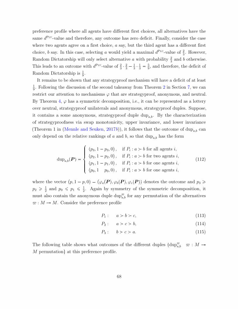
preference profile where all agents have different first choices, all alternatives have the
same dPlu-value and therefore, any outcome has zero deficit. Finally, consider the case
where two agents agree on a first choice, a say, but the third agent has a different first
choice, b say. In this case, selecting a would yield a maximal dPlu-value of 23. However,
Random Dictatorship will only select alternative a with probability 23
and b otherwise.
This leads to an outcome with dPlu-value of 23� 2
3� 1
3� 1
3� 5
9, and therefore, the deficit of
Random Dictatorship is 19.
It remains to be shown that any strategyproof mechanism will have a deficit of at least19. Following the discussion of the second takeaway from Theorem 2 in Section 7, we can
restrict our attention to mechanisms ϕ that are strategyproof, anonymous, and neutral.
By Theorem 4, ϕ has a symmetric decomposition, i.e., it can be represented as a lottery
over neutral, strategyproof unilaterals and anonymous, strategyproof duples. Suppose,
it contains a some anonymous, strategyproof duple dupa,b. By the characterization
of strategyproofness via swap monotonicity, upper invariance, and lower invariance
(Theorem 1 in (Mennle and Seuken, 2017b)), it follows that the outcome of dupa,b can
only depend on the relative rankings of a and b, so that dupa,b has the form
dupa,bpP q �
$''''&''''%
pp3, 1� p3, 0q , if Pi : a ¡ b for all agents i,
pp2, 1� p2, 0q , if Pi : a ¡ b for two agents i,
pp1, 1� p1, 0q , if Pi : a ¡ b for one agents i,
pp0, 1� p0, 0q , if Pi : a ¡ b for one agents i,
(112)
where the vector pp, 1 � p, 0q � pϕapP q, ϕbpP q, ϕcpP qq denotes the outcome and p3 ¥
p2 ¥ 12
and p0 ¤ p1 ¤ 12. Again by symmetry of the symmetric decomposition, it
must also contain the anonymous duple dup$a,b for any permutation of the alternatives
$ : M ÑM . Consider the preference profile
P1 : a ¡ b ¡ c, (113)
P2 : a ¡ c ¡ b, (114)
P3 : b ¡ c ¡ a. (115)
The following table shows what outcomes of the different duples tdup$a,b | $ : M Ñ
M permutationu at this preference profile.
68
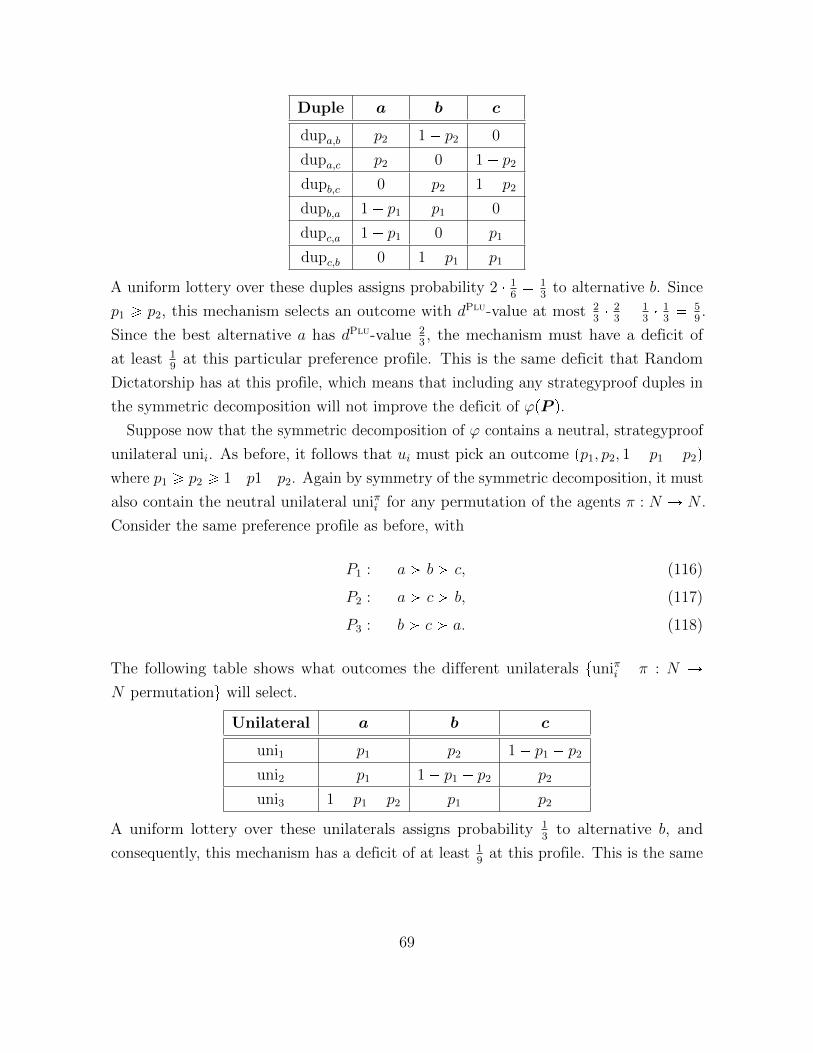
Duple a b c
dupa,b p2 1� p2 0
dupa,c p2 0 1� p2
dupb,c 0 p2 1� p2
dupb,a 1� p1 p1 0
dupc,a 1� p1 0 p1
dupc,b 0 1� p1 p1
A uniform lottery over these duples assigns probability 2 � 16� 1
3to alternative b. Since
p1 ¥ p2, this mechanism selects an outcome with dPlu-value at most 23� 2
3� 1
3� 1
3� 5
9.
Since the best alternative a has dPlu-value 23, the mechanism must have a deficit of
at least 19
at this particular preference profile. This is the same deficit that Random
Dictatorship has at this profile, which means that including any strategyproof duples in
the symmetric decomposition will not improve the deficit of ϕpP q.
Suppose now that the symmetric decomposition of ϕ contains a neutral, strategyproof
unilateral unii. As before, it follows that ui must pick an outcome pp1, p2, 1� p1 � p2q
where p1 ¥ p2 ¥ 1�p1�p2. Again by symmetry of the symmetric decomposition, it must
also contain the neutral unilateral uniπi for any permutation of the agents π : N Ñ N .
Consider the same preference profile as before, with
P1 : a ¡ b ¡ c, (116)
P2 : a ¡ c ¡ b, (117)
P3 : b ¡ c ¡ a. (118)
The following table shows what outcomes the different unilaterals tuniπi | π : N Ñ
N permutationu will select.
Unilateral a b c
uni1 p1 p2 1� p1 � p2
uni2 p1 1� p1 � p2 p2
uni3 1� p1 � p2 p1 p2
A uniform lottery over these unilaterals assigns probability 13
to alternative b, and
consequently, this mechanism has a deficit of at least 19
at this profile. This is the same
69
deficit that Random Dictatorship has at this profile, which means that including any
strategyproof unilaterals in the symmetric decomposition will not improve the deficit of
ϕpP q.
Since for all mechanisms the worst-case deficit was attained at the same preference
profile, there exists no strategyproof, anonymous, neutral mechanism that has a lower
deficit at P than 19, and therefore, Random Dictatorship has minimal deficit among all
strategyproof mechanisms.
Next, we show that the manipulability of Uniform Plurality is minimal among all dPlu-
maximizing mechanisms. Without loss of generality, we restrict attention to anonymous,
neutral, and dPlu-maximizing mechanisms. At any preference profile where an alternative
is ranked first by two agents or more, this alternative is implemented with certainty.
Thus, if two agents have the same first choice, the third agent has no opportunity to
manipulate, because it cannot change the outcome. The two agents with the same first
choice are already receiving their favorite outcome, which makes manipulation useless
for them as well.
Thus, any manipulability will arise at a preference profile where all agents have different
first choices. Consider the preference profile P with
P1 : a ¡ b ¡ c, (119)
P2 : b ¡ c ¡ a, (120)
P3 : c ¡ a ¡ b. (121)
Renaming the alternatives is equivalent to renaming the agents. Thus, an anonymous
and neutral mechanisms has to treat all alternatives equally and must therefore select
each alternative with probability 13. Now suppose that agent 1 is almost indifferent
between a and b, but strongly dislikes c, i.e., its utility function is “close to” the binary
utility upaq � upbq � 1, upcq � 0. Then, by swapping a and b, agent 1 can enforce the
implementation b with certainty. Its gain from this manipulation is close to
1 � upbq �1
3pupaq � upbq � upcqq �
1
3. (122)
Thus, any dPlu-maximizing mechanism will have manipulability εpϕq ¥ 13.
Now consider the Uniform Plurality mechanism. At the above preference profile agents
70
cannot change the outcome, unless they change their first choice. By anonymity and
neutrality, it suffices to show that agent 1 cannot do any better than 13
by manipulating.
However, the only other possible misreport that has any effect on the outcome is to
bring c forward and enforce it as the outcome, which would yield no benefit for agent 1.
Consequently, Uniform Plurality has minimal manipulability of 13.
Finally, we show that there are no additional supporting manipulability bounds besides
0 and 1{3. So far we have that Random Dictatorship is in Optp0q with a deficit of
δp0q � 19. Furthermore, Uniform Plurality is in Optp1{3q and no dPlu-maximizing
mechanism has strictly lower manipulability. To complete the proof, we will show that
for ε � 16, all optimal mechanisms have deficit 1
18. By convexity of the mapping ε ÞÑ δpεq,
the signature of the Pareto frontier must therefore be a straight line between p0, 1{9q
and p1{3, 0q. Considering the performance guarantees for hybrid mechanisms (Theorem
2), this implies optimality of the hybrids of Random Dictatorship and Uniform Plurality.
Suppose that ϕ is 16-approximately strategyproof, anonymous, and neutral. It follows
from anonymity and neutrality that at the preference profile
P1 : a ¡ b ¡ c, (123)
P2 : b ¡ c ¡ a, (124)
P3 : c ¡ a ¡ b, (125)
the outcome must be�
13, 1
3, 1
3
�for a, b, c, respectively. If agent 1 changes its report to
P 11 : b ¡ a ¡ c, (126)
the outcome changes to�
13� εa,
13� εa � εc,
13� εc
�for some values εa ¤
13, εc ¤
13.
Suppose now that agent 1 has a utility close to indifference between a and b, i.e., close
to upaq � upbq � 1, upcq � 0. Then the utility gain for agent 1 from misreporting P 11 is
(arbitrarily close to)
1 � p�εaq � 1 � pεa � εcq � 0 � p�εcq � εc. (127)
If the mechanism is 16-approximately strategyproof, then εc ¤
16. The dPlu-value of ϕpP 1q
71
at P 1 � pP 11, P2, P3q is
@ϕpP 1q, dPlup�,P 1q
D� ϕapP
1q � 0� ϕbpP1q �
2
3� ϕcpP
1q �1
3(128)
�2
3
�1
3� εa � εc
�
1
3
�1
3� εc
(129)
�6
18�
4
6εa �
1
3εc (130)
¤6
18�
4
18�
1
18�
11
18. (131)
However, the only dPlu-maximizing alternative at P 1 is b with dPlupb,P 1q � 23� 12
18.
Thus, any 16-approximately strategyproof mechanism must incur a deficit of at least
118
.
F.7. Proof of Proposition 5
Proof of Proposition 5. In a problem pN,M, δVetoq with n � 3 agents, m � 3 alterna-
tives, strict preferences, and where δVeto is the worst-case dVeto-deficit, the following
hold:
1. The Pareto frontier has four supporting manipulability bounds 0, 1{21, 1{12, 1{2.
2. Random Duple is a representative of Optp0q.
3. Uniform Veto is a representative of Optp1{2q.
4. Hybrids of Random Duple and Uniform Veto not optimal for β P p0, 1{2q.
First, we prove that Random Duple is optimal at ε0 � 0. Since it is a lottery over
strategyproof duple mechanisms, it is obviously strategyproof.
At any preference profile where all agents agree on the last choice, Random Duple
selects one of the other alternatives, each of which gives maximal dVeto-value. At any
preference profile where all agents have different last choices, any outcome has zero
deficit. Finally, consider a preference profile with
P1, P2 : . . . ¡ c, (132)
P3 : . . . ¡ b. (133)
72
The dVeto-value of a is 1 and the dVeto-value of b is 23, so that the maximum dVeto-value
is 1. The worst case for Random Duple is that agents 1 and 2 rank b first, in which
case a will be selected with probability 13
and b with probability 23. Thus, the deficit of
Random Duple at P is
1�1
3� 1�
2
3�
2
3�
2
9. (134)
In particular, this deficit is attained by Random Duple at the preference profile P with
P1, P2 : b ¡ a ¡ c, (135)
P3 : c ¡ a ¡ b. (136)
It remains to be proven whether any strategyproof, anonymous, neutral mechanism ϕ
can achieve a lower deficit (where anonymity and neutrality are without loss of generality,
similar to the proof of Proposition 4). Consider the preference profile P and let unii be
a strategyproof and neutral unilateral component in the symmetric decomposition of
ϕ. unii must pick an outcome pp1, p2, 1� p1 � p2q with p1 ¥ p2 ¥ 1� p1 � p2, where pk
denotes the probability of agent i’s kth choice. The symmetric decomposition implies
that uni1, uni2, and uni3 are equally likely to be chosen. Analogous to the proof of
Proposition 4, we get
Unilateral a b c
uni1 or uni2 p1 p2 1� p1 � p2
uni3 p2 1� p1 � p2 p1
Thus, alternative b is selected with probably at least 13, which means that the deficit of ϕ
at the preference profile P is not reduced by including any unilaterals in the symmetric
decomposition.
Similarly, if dupa,b is a strategyproof, anonymous duple in the symmetric decomposition
of ϕ, it has the form
dupa,bpP q �
$''''&''''%
pp3, 1� p3, 0q , if Pi : a ¡ b for all agents i,
pp2, 1� p2, 0q , if Pi : a ¡ b for two agents i,
pp1, 1� p1, 0q , if Pi : a ¡ b for one agents i,
pp0, 1� p0, 0q , if Pi : a ¡ b for one agents i,
(137)
73
where p3 ¥ p2 ¥12
and p0 ¤ p1 ¤12. Again by symmetry of the symmetric decomposition,
it must also contain the anonymous duple dup$a,b for any permutation of the alternatives
$ : M ÑM . The following table shows what outcomes the different duples tdup$a,b | $ :
M ÑM permutationu will select at P .
Duple a b c
dupa,b p1 1� p1 0
dupa,c p2 0 1� p2
dupb,c 0 p2 1� p2
dupb,a 1� p2 p2 0
dupc,a 1� p1 0 p1
dupc,b 0 1� p1 p1
Thus, since p2 ¥ p1, b is selected with probability of at least 13, and therefore, including
any other duples in the symmetric decomposition of ϕ will not improve the deficit at
P . Consequently, there exists no strategyproof mechanism with a lower deficit than
Random Duple.
Next, we show that Uniform Veto has minimal manipulability of among all dVeto-
maximizing mechanisms. First, observe that Uniform Veto is 12-approximately strate-
gyproof. To see this, consider the preference profile P
P1 : a ¡ b ¡ c, (138)
P2, P3 : . . . ¡ c. (139)
Uniform Veto selects a and b with probability 12
each. To manipulate, agent 1 can rank
b last and obtain a with certainty. Its gain from this manipulation would be
u1paq �1
2pu1paq � u1pbqq �
1
2pu1paq � u1pbqq , (140)
which is at most 12
for u1paq � 1 and u1pbq close to 0. Thus, the manipulability of
Uniform Veto is at least 12.
Suppose now that all agents have different last choices. In this case, Uniform Veto
selects any of the alternatives with probability 13. By ranking another alternative last,
an agent could only ensure the implementation of its third choice with certainty, which
74
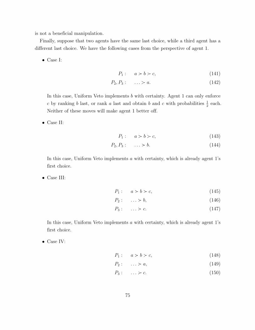
is not a beneficial manipulation.
Finally, suppose that two agents have the same last choice, while a third agent has a
different last choice. We have the following cases from the perspective of agent 1.
• Case I:
P1 : a ¡ b ¡ c, (141)
P2, P3 : . . . ¡ a. (142)
In this case, Uniform Veto implements b with certainty. Agent 1 can only enforce
c by ranking b last, or rank a last and obtain b and c with probabilities 12
each.
Neither of these moves will make agent 1 better off.
• Case II:
P1 : a ¡ b ¡ c, (143)
P2, P3 : . . . ¡ b. (144)
In this case, Uniform Veto implements a with certainty, which is already agent 1’s
first choice.
• Case III:
P1 : a ¡ b ¡ c, (145)
P2 : . . . ¡ b, (146)
P3 : . . . ¡ c. (147)
In this case, Uniform Veto implements a with certainty, which is already agent 1’s
first choice.
• Case IV:
P1 : a ¡ b ¡ c, (148)
P2 : . . . ¡ a, (149)
P3 : . . . ¡ c. (150)
75
In this case, Uniform Veto implements b with certainty. By ranking b last, agent
1 could obtain a probability of 13
for each alternative instead. Its gain from this
manipulation is
1
3pu1paq � u1pbq � u1pcqq � u1pbq ¤
1
3�
2
3u1pbq ¤
1
3. (151)
Further observe that by renaming agents and alternatives, the above cases I through IV
cover all possible constellations with 2 different alternatives ranked as last choices from
the perspective of any agent. Thus, Uniform Veto is 12-approximately strategyproof.
Having shown that the manipulability of Uniform Veto is exactly 12, we now must
show that any other dVeto-maximizing mechanism ϕ has manipulability εpϕq ¥ 12. We
assume without loss of generality that ϕ is also anonymous and neutral, and we consider
the preference profile
P1, P2 : a ¡ b ¡ c, (152)
P3 : b ¡ a ¡ c. (153)
At this profile, ϕ has to select a with some probability pa and b with probability 1�pa. If
pa ¥12, agent 3 can rank a last and enforce selection of b, the only remaining alternative
with full dVeto-value. If u3pbq � 1, u3pcq � 0, and u3paq is close to 0, its gain will be
1� p1� paq � pa ¥1
2. (154)
If pa 12, agent 1 can enforce a by ranking b last and obtain a gain of
1� pa ¡1
2(155)
with a similar utility function. Thus, any dVeto-maximizing mechanism has manipulability
of at least 12.
Last, we show that the hybrids of Random Duples and Uniform Veto do not lie on the
Pareto frontier, except for the extreme cases. In fact, the signatures of their hybrids form
a straight line: observe that the deficit of Random Duple is attained at the preference
76
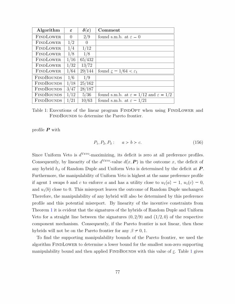
Algorithm ε δpεq Comment
FindLower 0 2{9 found s.m.b. at ε � 0FindLower 1{2 0FindLower 1{4 1{12FindLower 1{8 1{8FindLower 1{16 65{432FindLower 1{32 13{72FindLower 1{64 29{144 found ε � 1{64 ε1
FindBounds 1{6 1{9FindBounds 1{18 25{162FindBounds 3{47 28{187FindBounds 1{12 5{36 found s.m.b. at ε � 1{12 and ε � 1{2FindBounds 1{21 10{63 found s.m.b. at ε � 1{21
Table 1: Executions of the linear program FindOpt when using FindLower andFindBounds to determine the Pareto frontier.
profile P with
P1, P2, P3 : a ¡ b ¡ c. (156)
Since Uniform Veto is dVeto-maximizing, its deficit is zero at all preference profiles.
Consequently, by linearity of the dVeto-value dpx,P q in the outcome x, the deficit of
any hybrid hβ of Random Duple and Uniform Veto is determined by the deficit at P .
Furthermore, the manipulability of Uniform Veto is highest at the same preference profile
if agent 1 swaps b and c to enforce a and has a utility close to u1paq � 1, u1pcq � 0,
and u1pbq close to 0. This misreport leaves the outcome of Random Duple unchanged.
Therefore, the manipulability of any hybrid will also be determined by this preference
profile and this potential misreport. By linearity of the incentive constraints from
Theorem 1 it is evident that the signatures of the hybrids of Random Duple and Uniform
Veto for a straight line between the signatures p0, 2{9q and p1{2, 0q of the respective
component mechanism. Consequently, if the Pareto frontier is not linear, then these
hybrids will not be on the Pareto frontier for any β � 0, 1.
To find the supporting manipulability bounds of the Pareto frontier, we used the
algorithm FindLower to determine a lower bound for the smallest non-zero supporting
manipulability bound and then applied FindBounds with this value of ε. Table 1 gives
77
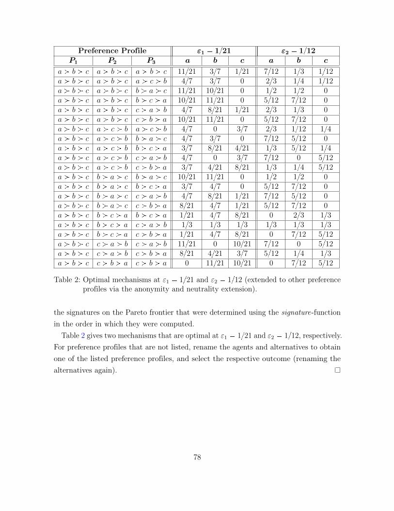
Preference Profile ε1 � 1{21 ε2 � 1{12P1 P2 P3 a b c a b c
a ¡ b ¡ c a ¡ b ¡ c a ¡ b ¡ c 11{21 3{7 1{21 7{12 1{3 1{12a ¡ b ¡ c a ¡ b ¡ c a ¡ c ¡ b 4{7 3{7 0 2{3 1{4 1{12a ¡ b ¡ c a ¡ b ¡ c b ¡ a ¡ c 11{21 10{21 0 1{2 1{2 0a ¡ b ¡ c a ¡ b ¡ c b ¡ c ¡ a 10{21 11{21 0 5{12 7{12 0a ¡ b ¡ c a ¡ b ¡ c c ¡ a ¡ b 4{7 8{21 1{21 2{3 1{3 0a ¡ b ¡ c a ¡ b ¡ c c ¡ b ¡ a 10{21 11{21 0 5{12 7{12 0a ¡ b ¡ c a ¡ c ¡ b a ¡ c ¡ b 4{7 0 3{7 2{3 1{12 1{4a ¡ b ¡ c a ¡ c ¡ b b ¡ a ¡ c 4{7 3{7 0 7{12 5{12 0a ¡ b ¡ c a ¡ c ¡ b b ¡ c ¡ a 3{7 8{21 4{21 1{3 5{12 1{4a ¡ b ¡ c a ¡ c ¡ b c ¡ a ¡ b 4{7 0 3{7 7{12 0 5{12a ¡ b ¡ c a ¡ c ¡ b c ¡ b ¡ a 3{7 4{21 8{21 1{3 1{4 5{12a ¡ b ¡ c b ¡ a ¡ c b ¡ a ¡ c 10{21 11{21 0 1{2 1{2 0a ¡ b ¡ c b ¡ a ¡ c b ¡ c ¡ a 3{7 4{7 0 5{12 7{12 0a ¡ b ¡ c b ¡ a ¡ c c ¡ a ¡ b 4{7 8{21 1{21 7{12 5{12 0a ¡ b ¡ c b ¡ a ¡ c c ¡ b ¡ a 8{21 4{7 1{21 5{12 7{12 0a ¡ b ¡ c b ¡ c ¡ a b ¡ c ¡ a 1{21 4{7 8{21 0 2{3 1{3a ¡ b ¡ c b ¡ c ¡ a c ¡ a ¡ b 1{3 1{3 1{3 1{3 1{3 1{3a ¡ b ¡ c b ¡ c ¡ a c ¡ b ¡ a 1{21 4{7 8{21 0 7{12 5{12a ¡ b ¡ c c ¡ a ¡ b c ¡ a ¡ b 11{21 0 10{21 7{12 0 5{12a ¡ b ¡ c c ¡ a ¡ b c ¡ b ¡ a 8{21 4{21 3{7 5{12 1{4 1{3a ¡ b ¡ c c ¡ b ¡ a c ¡ b ¡ a 0 11{21 10{21 0 7{12 5{12
Table 2: Optimal mechanisms at ε1 � 1{21 and ε2 � 1{12 (extended to other preferenceprofiles via the anonymity and neutrality extension).
the signatures on the Pareto frontier that were determined using the signature-function
in the order in which they were computed.
Table 2 gives two mechanisms that are optimal at ε1 � 1{21 and ε2 � 1{12, respectively.
For preference profiles that are not listed, rename the agents and alternatives to obtain
one of the listed preference profiles, and select the respective outcome (renaming the
alternatives again).
78
Recommended