Öncel Akademi: İstatistiksel Sismoloji

859

Bulletin of the Seismological Society of America, 90, 4, pp. 859–869, August 2000

Minimum Magnitude of Completeness in Earthquake Catalogs:

Examples from Alaska, the Western United States, and Japan

by Stefan Wiemer and Max Wyss

Abstract We mapped the minimum magnitude of complete reporting, Mc, forAlaska, the western United States, and for the JUNEC earthquake catalog of Japan.Mc was estimated based on its departure from the linear frequency-magnitude relationof the 250 closest earthquakes to grid nodes, spaced 10 km apart. In all catalogsstudied, Mc was strongly heterogeneous. In offshore areas the Mc was typically oneunit of magnitude higher than onshore. On land also, Mc can vary by one order ofmagnitude over distance less than 50 km. We recommend that seismicity studies thatdepend on complete sets of small earthquakes should be limited to areas with similarMc, or the minimum magnitude for the analysis has to be raised to the highest com-mon value of Mc. We believe that the data quality, as reflected by the Mc level, shouldbe used to define the spatial extent of seismicity studies where Mc plays a role. Themethod we use calculates the goodness of fit between a power law fit to the data andthe observed frequency-magnitude distribution as a function of a lower cutoff of themagnitude data. Mc is defined as the magnitude at which 90% of the data can bemodeled by a power law fit. Mc in the 1990s is approximately 1.2 � 0.4 in mostparts of California, 1.8 � 0.4 in most of Alaska (Aleutians and Panhandle excluded),and at a higher level in the JUNEC catalog for Japan. Various sources, such as ex-plosions and earthquake families beneath volcanoes, can lead to distributions thatcannot be fit well by power laws. For the Hokkaido region we demonstrate howneglecting the spatial variability of Mc can lead to erroneous assumptions aboutdeviations from self-similarity of earthquake scaling.

Introduction

The minimum magnitude of complete recording, Mc, isan important parameter for most studies related to seismicity.It is well known that Mc changes with time in most catalogs,usually decreasing, because the number of seismographs in-creases and the methods of analysis improve. However, dif-ferences of Mc as a function of space are generally ignored,although these, and the reasons for them, are just as obvious.For example, catalogs for offshore regions, as well asregions outside outer margins of the networks, are so radi-cally different in their reporting of earthquakes that theyshould not be used in quantitative studies together with thecatalogs for the central areas covered.

In seismicity studies, it is frequently necessary to usethe maximum number of events available for high-qualityresults. This objective is undermined if one uses a singleoverall Mc cutoff that is high, in order to guarantee com-pleteness. Here we show how a simple spatial mapping ofthe frequency-magnitude distribution (FMD) and applicationof a localized Mc cut-off can assist substantially in seismicitystudies. We demonstrate the benefits of spatial mapping ofMc for a number of case studies at a variety of scales.

For investigations of seismic quiescence and the fre-quency-magnitude relationship, we routinely map the min-imum magnitude of completeness to define an area of uni-form reporting for study (Wyss and Martyrosian, 1998,Wyss et al., 1999). Areas of inferior reporting (higher Mc),outside such a core area, are excluded because these datawould contaminate the analysis. In seismicity studies wherestatistical considerations play a key role, it is important thatresults are not influenced by the choice of the data limits. Ifthese limits are based on the catalog quality, then improvedstatistical robustness may be assured. For this reason we rou-tinely map the quality of the catalog for selecting the datafor our studies of seismic quiescence; however, homogeneityin Mc does not necessarily guarantee homogeneity in earth-quake reporting, since changes in magnitude reporting influ-ence the magnitude of homogeneous reporting (Habermann,1986; Habermann, 1991; Zuniga and Wyss, 1995; Zunigaand Wiemer, 1999).

Our estimation of Mc is based on the assumption that,for a given, volume a simple power law can approximate theFMD. The FMD (Ishimoto and Iida, 1939; Gutenberg and

860 S. Wiemer and M. Wyss

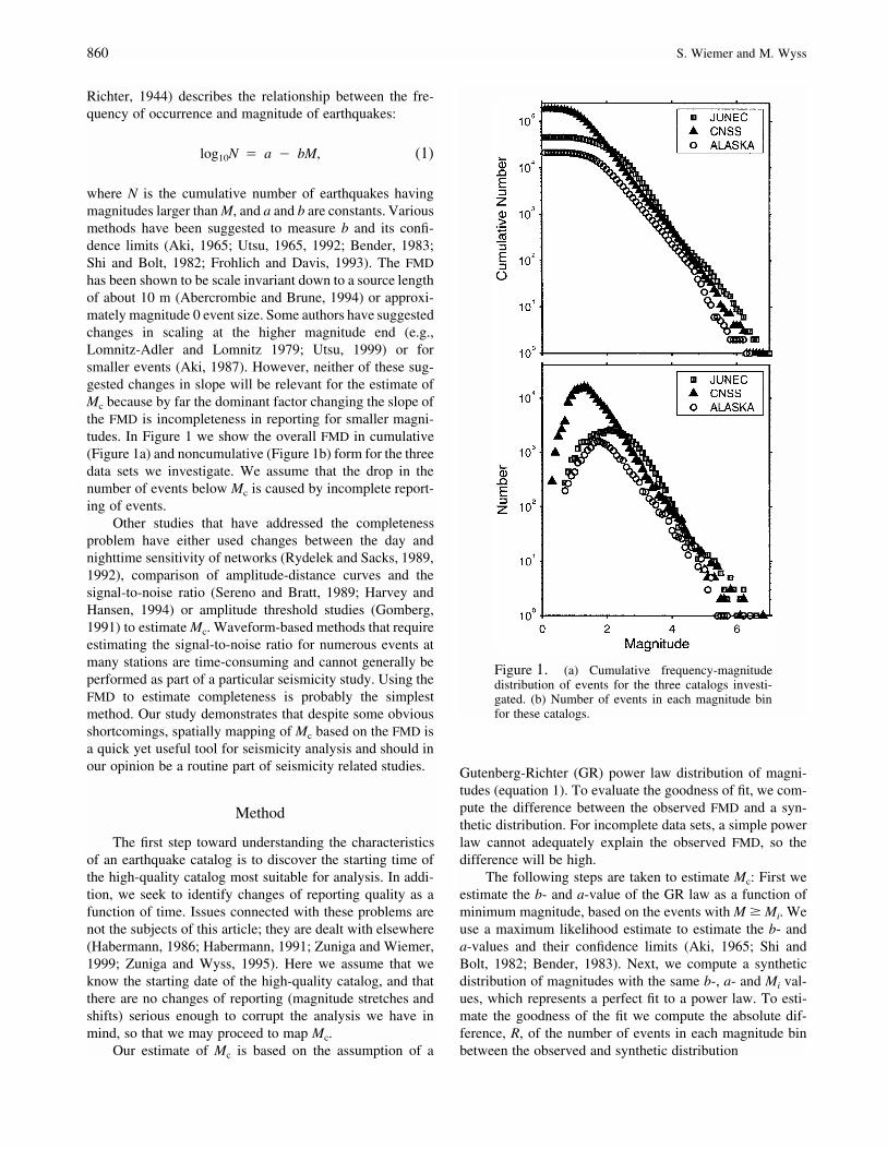
Figure 1. (a) Cumulative frequency-magnitudedistribution of events for the three catalogs investi-gated. (b) Number of events in each magnitude binfor these catalogs.

Richter, 1944) describes the relationship between the fre-quency of occurrence and magnitude of earthquakes:

log N � a � bM, (1)10

where N is the cumulative number of earthquakes havingmagnitudes larger than M, and a and b are constants. Variousmethods have been suggested to measure b and its confi-dence limits (Aki, 1965; Utsu, 1965, 1992; Bender, 1983;Shi and Bolt, 1982; Frohlich and Davis, 1993). The FMDhas been shown to be scale invariant down to a source lengthof about 10 m (Abercrombie and Brune, 1994) or approxi-mately magnitude 0 event size. Some authors have suggestedchanges in scaling at the higher magnitude end (e.g.,Lomnitz-Adler and Lomnitz 1979; Utsu, 1999) or forsmaller events (Aki, 1987). However, neither of these sug-gested changes in slope will be relevant for the estimate ofMc because by far the dominant factor changing the slope ofthe FMD is incompleteness in reporting for smaller magni-tudes. In Figure 1 we show the overall FMD in cumulative(Figure 1a) and noncumulative (Figure 1b) form for the threedata sets we investigate. We assume that the drop in thenumber of events below Mc is caused by incomplete report-ing of events.

Other studies that have addressed the completenessproblem have either used changes between the day andnighttime sensitivity of networks (Rydelek and Sacks, 1989,1992), comparison of amplitude-distance curves and thesignal-to-noise ratio (Sereno and Bratt, 1989; Harvey andHansen, 1994) or amplitude threshold studies (Gomberg,1991) to estimate Mc. Waveform-based methods that requireestimating the signal-to-noise ratio for numerous events atmany stations are time-consuming and cannot generally beperformed as part of a particular seismicity study. Using theFMD to estimate completeness is probably the simplestmethod. Our study demonstrates that despite some obviousshortcomings, spatially mapping of Mc based on the FMD isa quick yet useful tool for seismicity analysis and should inour opinion be a routine part of seismicity related studies.

Method

The first step toward understanding the characteristicsof an earthquake catalog is to discover the starting time ofthe high-quality catalog most suitable for analysis. In addi-tion, we seek to identify changes of reporting quality as afunction of time. Issues connected with these problems arenot the subjects of this article; they are dealt with elsewhere(Habermann, 1986; Habermann, 1991; Zuniga and Wiemer,1999; Zuniga and Wyss, 1995). Here we assume that weknow the starting date of the high-quality catalog, and thatthere are no changes of reporting (magnitude stretches andshifts) serious enough to corrupt the analysis we have inmind, so that we may proceed to map Mc.

Our estimate of Mc is based on the assumption of a

Gutenberg-Richter (GR) power law distribution of magni-tudes (equation 1). To evaluate the goodness of fit, we com-pute the difference between the observed FMD and a syn-thetic distribution. For incomplete data sets, a simple powerlaw cannot adequately explain the observed FMD, so thedifference will be high.

The following steps are taken to estimate Mc: First weestimate the b- and a-value of the GR law as a function ofminimum magnitude, based on the events with M � Mi. Weuse a maximum likelihood estimate to estimate the b- anda-values and their confidence limits (Aki, 1965; Shi andBolt, 1982; Bender, 1983). Next, we compute a syntheticdistribution of magnitudes with the same b-, a- and Mi val-ues, which represents a perfect fit to a power law. To esti-mate the goodness of the fit we compute the absolute dif-ference, R, of the number of events in each magnitude binbetween the observed and synthetic distribution

Minimum Magnitude of Completeness in Earthquake Catalogs: Examples from Alaska, the Western United States, and Japan 861

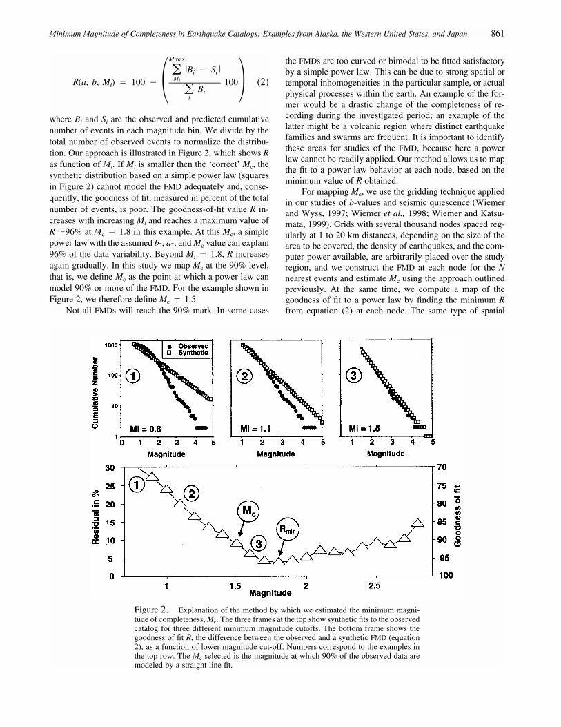
Figure 2. Explanation of the method by which we estimated the minimum magni-tude of completeness, Mc. The three frames at the top show synthetic fits to the observedcatalog for three different minimum magnitude cutoffs. The bottom frame shows thegoodness of fit R, the difference between the observed and a synthetic FMD (equation2), as a function of lower magnitude cut-off. Numbers correspond to the examples inthe top row. The Mc selected is the magnitude at which 90% of the observed data aremodeled by a straight line fit.

Mmax

|B � S |� i iMiR(a, b, M ) � 100 � 100 (2)i

B� �� ii

where Bi and Si are the observed and predicted cumulativenumber of events in each magnitude bin. We divide by thetotal number of observed events to normalize the distribu-tion. Our approach is illustrated in Figure 2, which shows Ras function of Mi. If Mi is smaller then the ‘correct’ Mc, thesynthetic distribution based on a simple power law (squaresin Figure 2) cannot model the FMD adequately and, conse-quently, the goodness of fit, measured in percent of the totalnumber of events, is poor. The goodness-of-fit value R in-creases with increasing Mi and reaches a maximum value ofR �96% at Mc � 1.8 in this example. At this Mc, a simplepower law with the assumed b-, a-, and Mc value can explain96% of the data variability. Beyond Mi � 1.8, R increasesagain gradually. In this study we map Mc at the 90% level,that is, we define Mc as the point at which a power law canmodel 90% or more of the FMD. For the example shown inFigure 2, we therefore define Mc � 1.5.

Not all FMDs will reach the 90% mark. In some cases

the FMDs are too curved or bimodal to be fitted satisfactoryby a simple power law. This can be due to strong spatial ortemporal inhomogeneities in the particular sample, or actualphysical processes within the earth. An example of the for-mer would be a drastic change of the completeness of re-cording during the investigated period; an example of thelatter might be a volcanic region where distinct earthquakefamilies and swarms are frequent. It is important to identifythese areas for studies of the FMD, because here a powerlaw cannot be readily applied. Our method allows us to mapthe fit to a power law behavior at each node, based on theminimum value of R obtained.

For mapping Mc, we use the gridding technique appliedin our studies of b-values and seismic quiescence (Wiemerand Wyss, 1997; Wiemer et al., 1998; Wiemer and Katsu-mata, 1999). Grids with several thousand nodes spaced reg-ularly at 1 to 20 km distances, depending on the size of thearea to be covered, the density of earthquakes, and the com-puter power available, are arbitrarily placed over the studyregion, and we construct the FMD at each node for the Nnearest events and estimate Mc using the approach outlinedpreviously. At the same time, we compute a map of thegoodness of fit to a power law by finding the minimum Rfrom equation (2) at each node. The same type of spatial


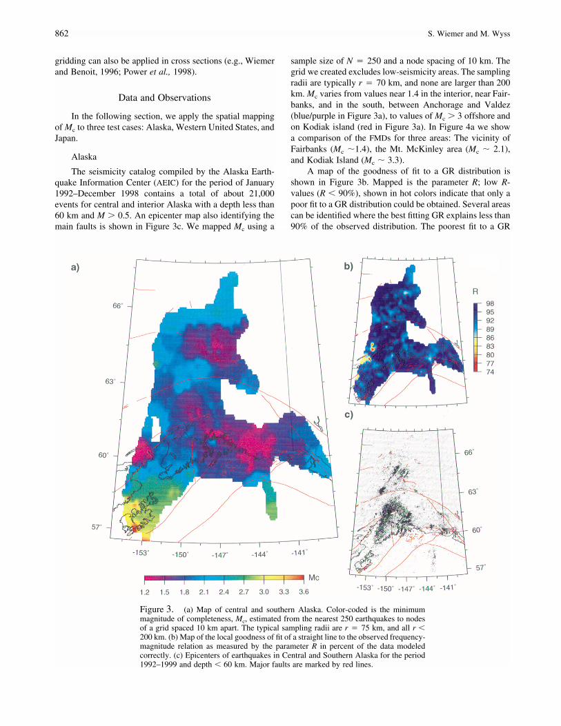
Figure 3. (a) Map of central and southern Alaska. Color-coded is the minimummagnitude of completeness, Mc, estimated from the nearest 250 earthquakes to nodesof a grid spaced 10 km apart. The typical sampling radii are r � 75 km, and all r �200 km. (b) Map of the local goodness of fit of a straight line to the observed frequency-magnitude relation as measured by the parameter R in percent of the data modeledcorrectly. (c) Epicenters of earthquakes in Central and Southern Alaska for the period1992–1999 and depth � 60 km. Major faults are marked by red lines.

gridding can also be applied in cross sections (e.g., Wiemerand Benoit, 1996; Power et al., 1998).

Data and Observations

In the following section, we apply the spatial mappingof Mc to three test cases: Alaska, Western United States, andJapan.

Alaska

The seismicity catalog compiled by the Alaska Earth-quake Information Center (AEIC) for the period of January1992–December 1998 contains a total of about 21,000events for central and interior Alaska with a depth less than60 km and M � 0.5. An epicenter map also identifying themain faults is shown in Figure 3c. We mapped Mc using a

sample size of N � 250 and a node spacing of 10 km. Thegrid we created excludes low-seismicity areas. The samplingradii are typically r � 70 km, and none are larger than 200km. Mc varies from values near 1.4 in the interior, near Fair-banks, and in the south, between Anchorage and Valdez(blue/purple in Figure 3a), to values of Mc � 3 offshore andon Kodiak island (red in Figure 3a). In Figure 4a we showa comparison of the FMDs for three areas: The vicinity ofFairbanks (Mc �1.4), the Mt. McKinley area (Mc � 2.1),and Kodiak Island (Mc � 3.3).

A map of the goodness of fit to a GR distribution isshown in Figure 3b. Mapped is the parameter R; low R-values (R � 90%), shown in hot colors indicate that only apoor fit to a GR distribution could be obtained. Several areascan be identified where the best fitting GR explains less than90% of the observed distribution. The poorest fit to a GR


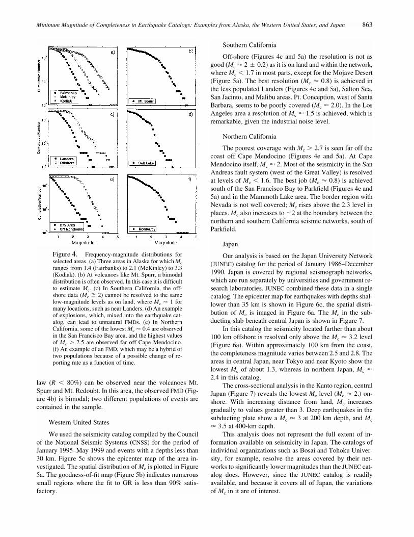
Figure 4. Frequency-magnitude distributions forselected areas. (a) Three areas in Alaska for which Mc

ranges from 1.4 (Fairbanks) to 2.1 (McKinley) to 3.3(Kodiak). (b) At volcanoes like Mt. Spurr, a bimodaldistribution is often observed. In this case it is difficultto estimate Mc. (c) In Southern California, the off-shore data (Mc � 2) cannot be resolved to the samelow-magnitude levels as on land, where Mc � 1 formany locations, such as near Landers. (d) An exampleof explosions, which, mixed into the earthquake cat-alog, can lead to unnatural FMDs. (e) In NorthernCalifornia, some of the lowest Mc � 0.4 are observedin the San Francisco Bay area, and the highest valuesof Mc � 2.5 are observed far off Cape Mendocino.(f) An example of an FMD, which may be a hybrid oftwo populations because of a possible change of re-porting rate as a function of time.

law (R � 80%) can be observed near the volcanoes Mt.Spurr and Mt. Redoubt. In this area, the observed FMD (Fig-ure 4b) is bimodal; two different populations of events arecontained in the sample.

Western United States

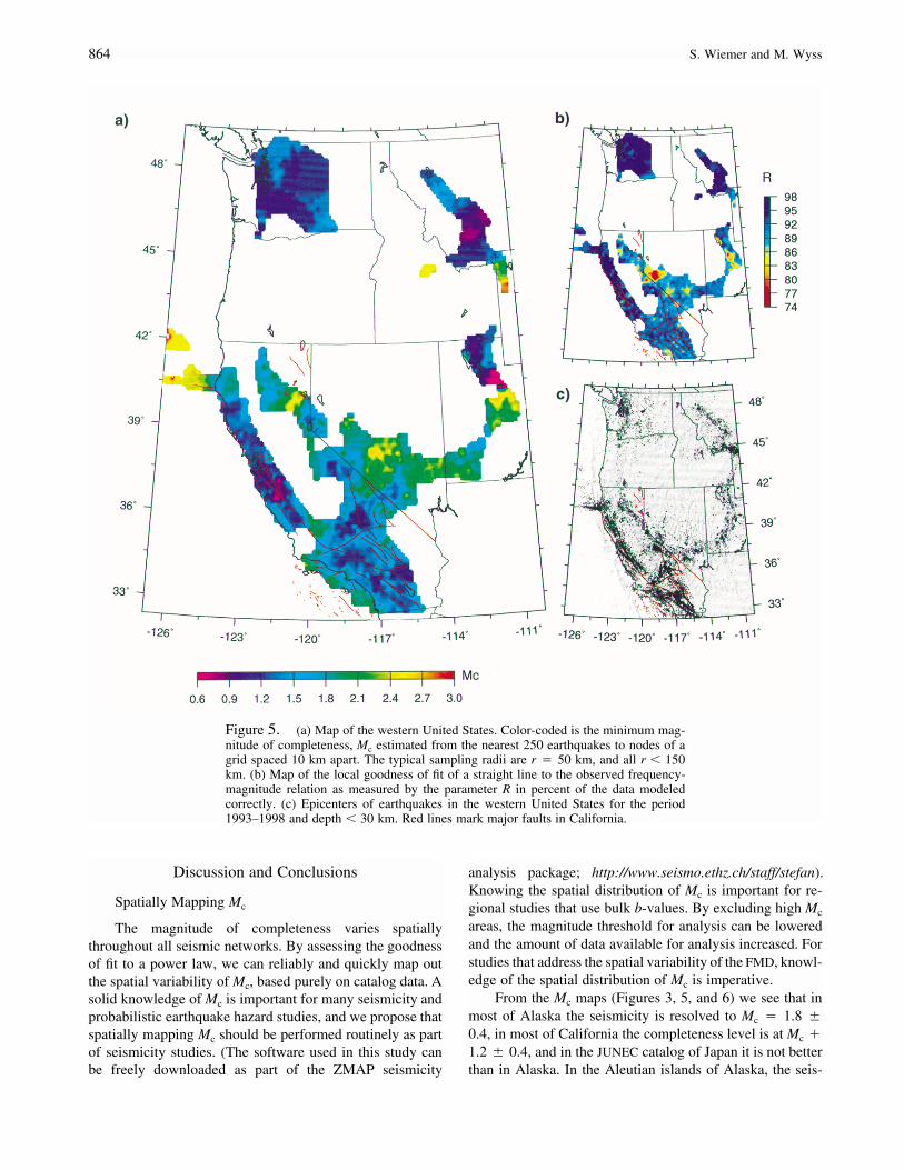
We used the seismicity catalog compiled by the Councilof the National Seismic Systems (CNSS) for the period ofJanuary 1995–May 1999 and events with a depths less than30 km. Figure 5c shows the epicenter map of the area in-vestigated. The spatial distribution of Mc is plotted in Figure5a. The goodness-of-fit map (Figure 5b) indicates numeroussmall regions where the fit to GR is less than 90% satis-factory.

Southern California

Off-shore (Figures 4c and 5a) the resolution is not asgood (Mc � 2 � 0.2) as it is on land and within the network,where Mc � 1.7 in most parts, except for the Mojave Desert(Figure 5a). The best resolution (Mc � 0.8) is achieved inthe less populated Landers (Figures 4c and 5a), Salton Sea,San Jacinto, and Malibu areas. Pt. Conception, west of SantaBarbara, seems to be poorly covered (Mc � 2.0). In the LosAngeles area a resolution of Mc � 1.5 is achieved, which isremarkable, given the industrial noise level.

Northern California

The poorest coverage with Mc � 2.7 is seen far off thecoast off Cape Mendocino (Figures 4e and 5a). At CapeMendocino itself, Mc � 2. Most of the seismicity in the SanAndreas fault system (west of the Great Valley) is resolvedat levels of Mc � 1.6. The best job (Mc � 0.8) is achievedsouth of the San Francisco Bay to Parkfield (Figures 4e and5a) and in the Mammoth Lake area. The border region withNevada is not well covered; Mc rises above the 2.3 level inplaces. Mc also increases to �2 at the boundary between thenorthern and southern California seismic networks, south ofParkfield.

Japan

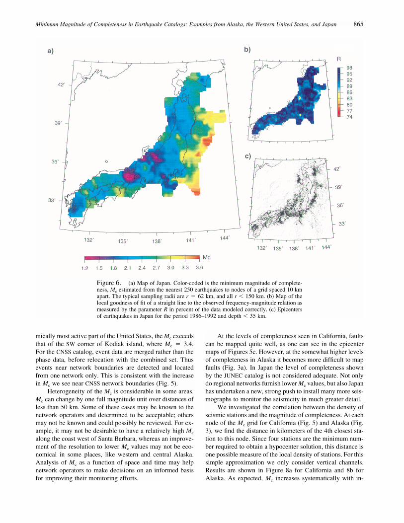
Our analysis is based on the Japan University Network(JUNEC) catalog for the period of January 1986–December1990. Japan is covered by regional seismograph networks,which are run separately by universities and government re-search laboratories. JUNEC combined these data in a singlecatalog. The epicenter map for earthquakes with depths shal-lower than 35 km is shown in Figure 6c, the spatial distri-bution of Mc is imaged in Figure 6a. The Mc in the sub-ducting slab beneath central Japan is shown in Figure 7.

In this catalog the seismicity located farther than about100 km offshore is resolved only above the Mc � 3.2 level(Figure 6a). Within approximately 100 km from the coast,the completeness magnitude varies between 2.5 and 2.8. Theareas in central Japan, near Tokyo and near Kyoto show thelowest Mc of about 1.3, whereas in northern Japan, Mc �2.4 in this catalog.

The cross-sectional analysis in the Kanto region, centralJapan (Figure 7) reveals the lowest Mc level (Mc � 2.) on-shore. With increasing distance from land, Mc increasesgradually to values greater than 3. Deep earthquakes in thesubducting plate show a Mc � 3 at 200 km depth, and Mc

� 3.5 at 400-km depth.This analysis does not represent the full extent of in-

formation available on seismicity in Japan. The catalogs ofindividual organizations such as Bosai and Tohoku Univer-sity, for example, resolve the areas covered by their net-works to significantly lower magnitudes than the JUNEC cat-alog does. However, since the JUNEC catalog is readilyavailable, and because it covers all of Japan, the variationsof Mc in it are of interest.


Figure 5. (a) Map of the western United States. Color-coded is the minimum mag-nitude of completeness, Mc estimated from the nearest 250 earthquakes to nodes of agrid spaced 10 km apart. The typical sampling radii are r � 50 km, and all r � 150km. (b) Map of the local goodness of fit of a straight line to the observed frequency-magnitude relation as measured by the parameter R in percent of the data modeledcorrectly. (c) Epicenters of earthquakes in the western United States for the period1993–1998 and depth � 30 km. Red lines mark major faults in California.

Discussion and Conclusions

Spatially Mapping Mc

The magnitude of completeness varies spatiallythroughout all seismic networks. By assessing the goodnessof fit to a power law, we can reliably and quickly map outthe spatial variability of Mc, based purely on catalog data. Asolid knowledge of Mc is important for many seismicity andprobabilistic earthquake hazard studies, and we propose thatspatially mapping Mc should be performed routinely as partof seismicity studies. (The software used in this study canbe freely downloaded as part of the ZMAP seismicity

analysis package; http://www.seismo.ethz.ch/staff/stefan).Knowing the spatial distribution of Mc is important for re-gional studies that use bulk b-values. By excluding high Mc

areas, the magnitude threshold for analysis can be loweredand the amount of data available for analysis increased. Forstudies that address the spatial variability of the FMD, knowl-edge of the spatial distribution of Mc is imperative.

From the Mc maps (Figures 3, 5, and 6) we see that inmost of Alaska the seismicity is resolved to Mc � 1.8 �0.4, in most of California the completeness level is at Mc �1.2 � 0.4, and in the JUNEC catalog of Japan it is not betterthan in Alaska. In the Aleutian islands of Alaska, the seis-


Figure 6. (a) Map of Japan. Color-coded is the minimum magnitude of complete-ness, Mc estimated from the nearest 250 earthquakes to nodes of a grid spaced 10 kmapart. The typical sampling radii are r � 62 km, and all r � 150 km. (b) Map of thelocal goodness of fit of a straight line to the observed frequency-magnitude relation asmeasured by the parameter R in percent of the data modeled correctly. (c) Epicentersof earthquakes in Japan for the period 1986–1992 and depth � 35 km.

mically most active part of the United States, the Mc exceedsthat of the SW corner of Kodiak island, where Mc � 3.4.For the CNSS catalog, event data are merged rather than thephase data, before relocation with the combined set. Thusevents near network boundaries are detected and locatedfrom one network only. This is consistent with the increasein Mc we see near CNSS network boundaries (Fig. 5).

Heterogeneity of the Mc is considerable in some areas.Mc can change by one full magnitude unit over distances ofless than 50 km. Some of these cases may be known to thenetwork operators and determined to be acceptable; othersmay not be known and could possibly be reviewed. For ex-ample, it may not be desirable to have a relatively high Mc

along the coast west of Santa Barbara, whereas an improve-ment of the resolution to lower Mc values may not be eco-nomical in some places, like western and central Alaska.Analysis of Mc as a function of space and time may helpnetwork operators to make decisions on an informed basisfor improving their monitoring efforts.

At the levels of completeness seen in California, faultscan be mapped quite well, as one can see in the epicentermaps of Figures 5c. However, at the somewhat higher levelsof completeness in Alaska it becomes more difficult to mapfaults (Fig. 3a). In Japan the level of completeness shownby the JUNEC catalog is not considered adequate. Not onlydo regional networks furnish lower Mc values, but also Japanhas undertaken a new, strong push to install many more seis-mographs to monitor the seismicity in much greater detail.

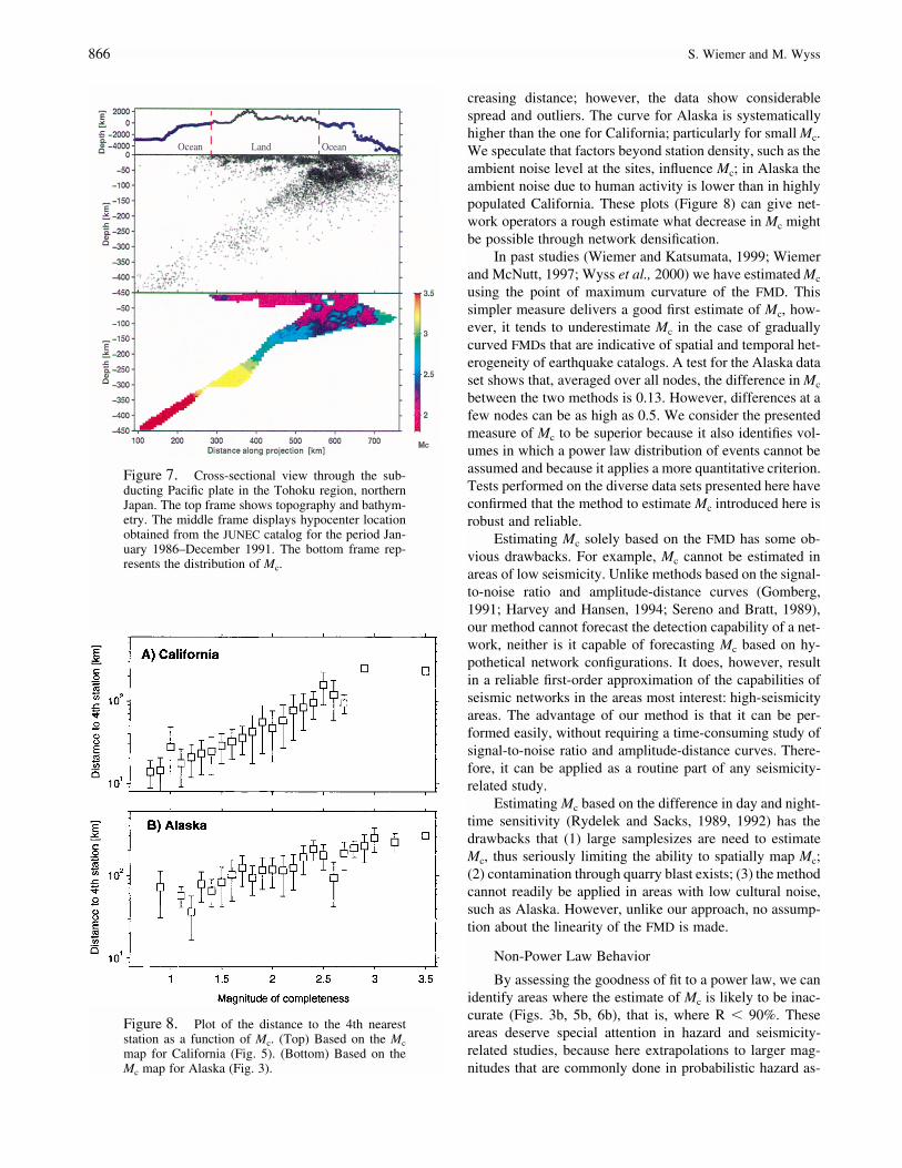
We investigated the correlation between the density ofseismic stations and the magnitude of completeness. At eachnode of the Mc grid for California (Fig. 5) and Alaska (Fig.3), we find the distance in kilometers of the 4th closest sta-tion to this node. Since four stations are the minimum num-ber required to obtain a hypocenter solution, this distance isone possible measure of the local density of stations. For thissimple approximation we only consider vertical channels.Results are shown in Figure 8a for California and 8b forAlaska. As expected, Mc increases systematically with in-


Figure 7. Cross-sectional view through the sub-ducting Pacific plate in the Tohoku region, northernJapan. The top frame shows topography and bathym-etry. The middle frame displays hypocenter locationobtained from the JUNEC catalog for the period Jan-uary 1986–December 1991. The bottom frame rep-resents the distribution of Mc.

Figure 8. Plot of the distance to the 4th neareststation as a function of Mc. (Top) Based on the Mc

map for California (Fig. 5). (Bottom) Based on theMc map for Alaska (Fig. 3).

creasing distance; however, the data show considerablespread and outliers. The curve for Alaska is systematicallyhigher than the one for California; particularly for small Mc.We speculate that factors beyond station density, such as theambient noise level at the sites, influence Mc; in Alaska theambient noise due to human activity is lower than in highlypopulated California. These plots (Figure 8) can give net-work operators a rough estimate what decrease in Mc mightbe possible through network densification.

In past studies (Wiemer and Katsumata, 1999; Wiemerand McNutt, 1997; Wyss et al., 2000) we have estimated Mc

using the point of maximum curvature of the FMD. Thissimpler measure delivers a good first estimate of Mc, how-ever, it tends to underestimate Mc in the case of graduallycurved FMDs that are indicative of spatial and temporal het-erogeneity of earthquake catalogs. A test for the Alaska dataset shows that, averaged over all nodes, the difference in Mc

between the two methods is 0.13. However, differences at afew nodes can be as high as 0.5. We consider the presentedmeasure of Mc to be superior because it also identifies vol-umes in which a power law distribution of events cannot beassumed and because it applies a more quantitative criterion.Tests performed on the diverse data sets presented here haveconfirmed that the method to estimate Mc introduced here isrobust and reliable.

Estimating Mc solely based on the FMD has some ob-vious drawbacks. For example, Mc cannot be estimated inareas of low seismicity. Unlike methods based on the signal-to-noise ratio and amplitude-distance curves (Gomberg,1991; Harvey and Hansen, 1994; Sereno and Bratt, 1989),our method cannot forecast the detection capability of a net-work, neither is it capable of forecasting Mc based on hy-pothetical network configurations. It does, however, resultin a reliable first-order approximation of the capabilities ofseismic networks in the areas most interest: high-seismicityareas. The advantage of our method is that it can be per-formed easily, without requiring a time-consuming study ofsignal-to-noise ratio and amplitude-distance curves. There-fore, it can be applied as a routine part of any seismicity-related study.

Estimating Mc based on the difference in day and night-time sensitivity (Rydelek and Sacks, 1989, 1992) has thedrawbacks that (1) large samplesizes are need to estimateMc, thus seriously limiting the ability to spatially map Mc;(2) contamination through quarry blast exists; (3) the methodcannot readily be applied in areas with low cultural noise,such as Alaska. However, unlike our approach, no assump-tion about the linearity of the FMD is made.

Non-Power Law Behavior

By assessing the goodness of fit to a power law, we canidentify areas where the estimate of Mc is likely to be inac-curate (Figs. 3b, 5b, 6b), that is, where R � 90%. Theseareas deserve special attention in hazard and seismicity-related studies, because here extrapolations to larger mag-nitudes that are commonly done in probabilistic hazard as-


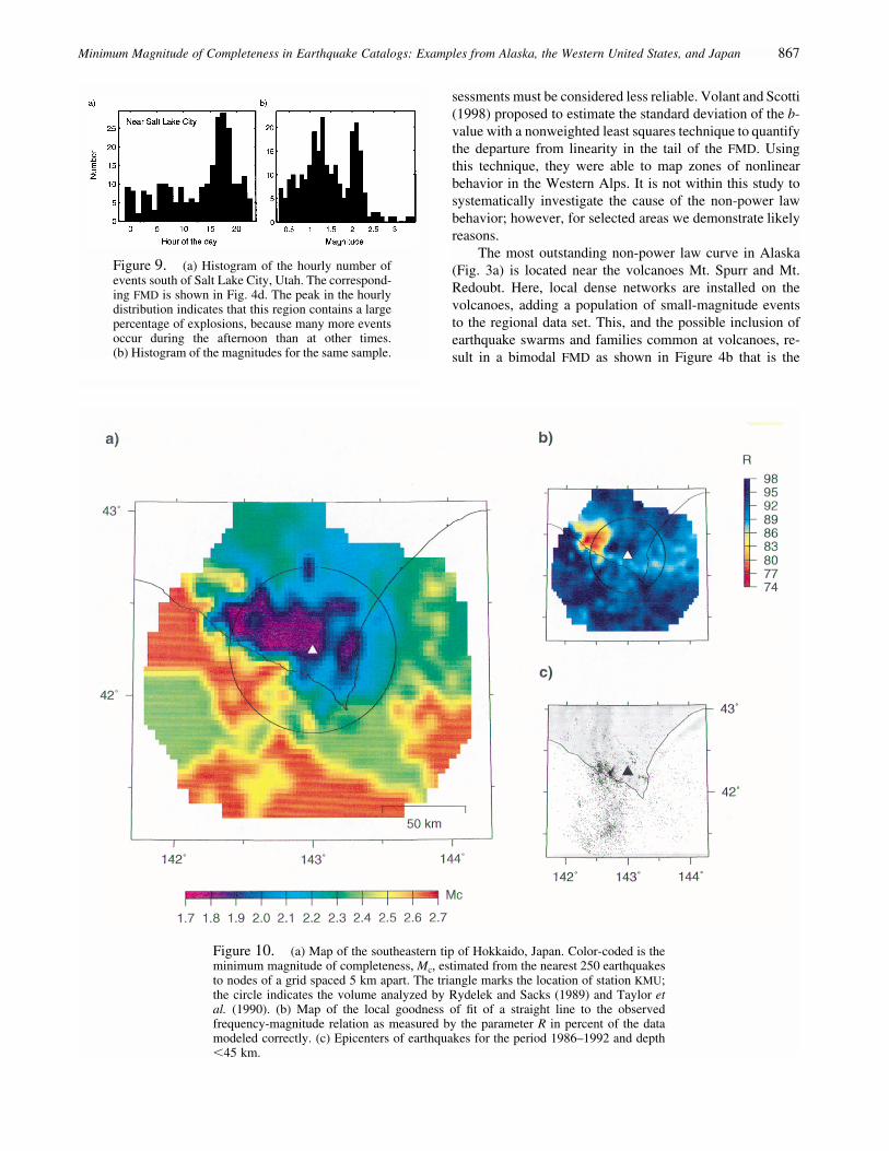
Figure 9. (a) Histogram of the hourly number ofevents south of Salt Lake City, Utah. The correspond-ing FMD is shown in Fig. 4d. The peak in the hourlydistribution indicates that this region contains a largepercentage of explosions, because many more eventsoccur during the afternoon than at other times.(b) Histogram of the magnitudes for the same sample.

sessments must be considered less reliable. Volant and Scotti(1998) proposed to estimate the standard deviation of the b-value with a nonweighted least squares technique to quantifythe departure from linearity in the tail of the FMD. Usingthis technique, they were able to map zones of nonlinearbehavior in the Western Alps. It is not within this study tosystematically investigate the cause of the non-power lawbehavior; however, for selected areas we demonstrate likelyreasons.

The most outstanding non-power law curve in Alaska(Fig. 3a) is located near the volcanoes Mt. Spurr and Mt.Redoubt. Here, local dense networks are installed on thevolcanoes, adding a population of small-magnitude eventsto the regional data set. This, and the possible inclusion ofearthquake swarms and families common at volcanoes, re-sult in a bimodal FMD as shown in Figure 4b that is the

Figure 10. (a) Map of the southeastern tip of Hokkaido, Japan. Color-coded is theminimum magnitude of completeness, Mc, estimated from the nearest 250 earthquakesto nodes of a grid spaced 5 km apart. The triangle marks the location of station KMU;the circle indicates the volume analyzed by Rydelek and Sacks (1989) and Taylor etal. (1990). (b) Map of the local goodness of fit of a straight line to the observedfrequency-magnitude relation as measured by the parameter R in percent of the datamodeled correctly. (c) Epicenters of earthquakes for the period 1986–1992 and depth�45 km.


telltale sign of combining populations of events with differ-ent properties.

In Utah we find low R-values south of Salt Lake City(Fig. 5b), and the respective FMD is shown in Figure 4d. Inthis region, we also notice a strong gradient in the Mc values(Fig. 5a). In a plot of the hourly distribution of events forthis volume (Fig. 9a), one notices a dominant peak duringdaytime hours, which is a telltale sign of blast activity(Wiemer and Baer, 2000). The combined FMD of the explo-sions that preferably scale around M2 (Fig. 9b) and naturalearthquake results in a strongly nonlinear behavior of theFMD.

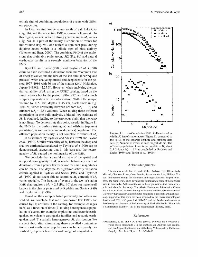
Rydelek and Sacks (1989) and Taylor et al. (1990)claim to have identified a deviation from the “common loreof linear b-values and the idea of the self similar earthquakeprocess” when analyzing crustal and deep events for the pe-riod 1977–1986 with 50 km of the station KMU, Hokkaido,Japan (143.0 E, 42.25 N). However, when analyzing the spa-tial variability of Mc using the JUNEC catalog, based on thesame network but for the period 1986–1992, we find a muchsimpler explanation of their observation: Within the samplevolume (R � 50 km, depths � 45 km, black circle in Fig.10a), Mc varies drastically between onshore (Mc � 1.8) andoffshore (Mc � 2.5) volumes. When mixing these differentpopulations in one bulk analysis, a biased, low estimate ofMc is obtained, leading to the erroneous claim that the FMDis not linear. To demonstrate this point, we plot in Figure 11the FMD for the onshore (triangles) and offshore (squares)population, as well as the combined (circles) population. Theoffshore population clearly is not complete to values of Mc

� 1.8 as assumed by Rydelek and Sacks (1989) and Tayloret al. (1990). Similar variability of Mc between the deep andshallow earthquakes analyzed by Taylor et al. (1990) can bedemonstrated, suggesting that in this case also the hetero-geneity of Mc caused the nonlinearity of the FMD.

We conclude that a careful estimate of the spatial andtemporal homogeneity of Mc is needed before any claim ofdeviations from a power law behavior for small magnitudescan be made. The daytime to nighttime activity variationcriteria applied in Rydelek and Sacks (1989) and Taylor etal. (1990) do not seem able to determine Mc correctly if Mc

varies spatially. The fraction of events to the SW of stationKMU that requires a Mc � 2.5 (Fig. 10) does not make itselfknown in the phasor plots used by Rydelek and Sacks (1989)and Taylor et al. (1990).

Based on the examples listed previously and others westudied, we conclude that most non-power law FMDs arecaused by (1) artifacts in the catalog, for example, changesin Mc as a function of time; (2) mixing heterogeneous popu-lation of events, for example, explosions and tectonic earth-quakes, or volcanic earthquake families and tectonic earth-quakes; and (3) spatially heterogeneous Mc distribution. Wesuspect that, after eliminating these so-called contamina-tions, most earthquake populations can be adequately de-scribed by a power law for a wide range of magnitudes.

Acknowledgments

The authors would like to thank Walter Arabasz, Fred Klein, AndyMichael, Charlotte Rowe, Oona Scottie, Suzan van der Lee, Philippe Vo-lant, and Ramon Zuniga for comments and suggestions that helped to im-prove the manuscript. Yuzo Toya helped to implement some of the softwareused in this study. Additional thanks to the organizations that made avail-able their data for this study: The Alaska Earthquake Information Centerand the NCEDC and its contributing institutions and the Japanese NationalUniversity Earthquake Consortium for producing a national earthquake cat-alog. Support for this work has been provided by the Swiss SeismologicalService and ETH, NSF grant EAR 9614783 and the Wadati endowment atthe Geophysical Institute of the University of Alaska Fairbanks. This articleis Contribution Number 1111 of the Geophysical Institute, ETHZ.

References

Abercrombie, R. E., and J. N. Brune (1994). Evidence for a constant b-value above magnitude 0 in the southern San Andreas, San Jacinto,and San Miguel fault zones and at the Long Valley caldera, California,Geophys. Res. Lett. 21, no. 15, 1647–1650.

Figure 11. (a) Cumulative FMD of all earthquakeswithin 50 km of station KMU (Figure 9), compared tothe FMDs of the separate onshore and offshore datasets. (b) Number of events in each magnitude bin. Theoffshore population of events is complete to Mc about2.5–2.8, not Mc � 1.8 as concluded by Rydelek andSacks (1989) and Taylor et al. (1990).


Aki, K. (1965). Maximum likelihood estimate of b in the formula log N �

a � bM and its confidence limits, Bull. Earthquake Res. Inst. 43,237–239.

Aki, K. (1987). Magnitude frequency relation for small earthquakes: a clueto the origin of fmax of large earthquakes, J. Geophys. Res. 92, 1349–1355.

Bender, B. (1983). Maximum likelihood estimation of b-values for mag-nitude grouped data, Bull. Seism. Soc. Am. 73, 831–851.

Frohlich, C., and S. Davis (1993). Teleseismic b-values: or, much ado about1.0, J. Geophys. Res. 98, 631–644.

Gomberg, J. (1991). Seismicity and detection/location threshold in thesouthern Great Basin seismic network, J. Geophys. Res. 96, no. B10,16,401–16,414.

Gutenberg, R., and C. F. Richter (1944). Frequency of earthquakes in Cali-fornia, Bull. Seism. Soc. Am. 34, 185–188.

Habermann, R. E. (1986). A test of two techniques for recognizing system-atic errors in magnitude estimates using data from Parkfield, Califor-nia, Bull. Seism. Soc. Am. 76, 1660–1667.

Habermann, R. E. (1991). Seismicity rate variations and systematic changesin magnitudes in teleseismic catalogs, Tectonophysics 193, 277–289.

Harvey, D., and R. Hansen (1994). Contributions of IRIS data to nuclearmonitoring, IRIS Newsletter 13, 1.

Ishimoto, M., and K. Iida (1939). Observations of earthquakes registeredwith the microseismograph constructed recently, Bull. EarthquakeRes. Inst. 17, 443–478.

Lomnitz-Adler, J., and C. Lomnitz (1979). A modified form of the Guten-berg-Richter magnitude-frequency relation, Bull. Seism. Soc. Am. 69,1209–1214.

Power, J. A., M. Wyss, and J. L. Latchman (1998). Spatial variations infrequency-magnitude distribution of earthquakes at Soufriere Hillsvolcano, Montserrat, West Indies, Geophys. Res. Lett. 25, 3653–3656.

Rydelek, P. A., and I. S. Sacks (1989). Testing the completeness of earth-quake catalogs and the hypothesis of self-similarity, Nature 337, 251–253.

Rydelek, P. A., and I. S. Sacks (1992). Comment on “Seismicity and de-tection/location threshold in the southern Great Basin seismic net-work” by Joan Gomberg, J. Geophys. Res. 97, no. B11, 15,361–15,362.

Sereno, T. J. Jr., and S. R. Bratt (1989). Seismic detection capability atNORESS and implications for the detection threshold of a hypotheticalnetwork in the Soviet Union, J. Geophys. Res. 94, no. B8, 10,397–10,414.

Shi, Y., and B. A. Bolt (1982). The standard error of the magnitude-frequency b value, Bull. Seism. Soc. Am. 72, 1677–1687.

Taylor, D. A., J. A. Snoke, I. S. Sacks, T. Takanami (1990). Nonlinearfrequency magnitude relationship for the Hokkaido corner, Japan,Bull. Seism. Soc. Am. 80, 340–353.

Utsu, T. (1965). A method for determining the value of b in a formula logn � a � bM showing the magnitude frequency for earthquakes,Geophys. Bull. Hokkaido Univ. 13, 99–103.

Utsu, T. (1992). On seismicity, In Report of the Joint Research Institutefor Statistical Mathematics, Institute for Statistical Mathematics, To-kyo, pp. 139–157.

Utsu, T. (1999). Representation and analysis of the earthquake size distri-bution: a historical review and some new approaches, Pure Appl Geo-phys 155, 471–507.

Volant, P., and O. Scotti (1998). Deviations from self-organized criticalstate: a case study in the Western Alps, EOS, Trans. Am. Geophys.Union, F648.

Wiemer, S. Stefan Wiemer’s Home Page, http://www.seismo.ethz.ch/staff/stefan

Wiemer, S., and M. Baer (2000). Mapping and removing quarry blast eventsfrom seismicity catalogs, Bull. Seism. Soc. Am. 90, 525–530.

Wiemer, S., and J. Benoit (1996). Mapping the b-value anomaly at 100 kmdepth in the Alaska and New Zealand subduction zones, Geophys.Res. Lett. 23, 1557–1560.

Wiemer, S., and K. Katsumata (1999). Spatial variability of seismicity pa-rameters in aftershock zones, J. Geophys. Res. 103, 13,135–13,151.

Wiemer, S., and S. McNutt (1997). Variations in frequency-magnitude dis-tribution with depth in two volcanic areas: Mount St. Helens, Wash-ington, and Mt. Spurr, Alaska, Geophys. Res. Lett. 24, 189–192.

Wiemer, S., and M. Wyss (1997). Mapping the frequency-magnitude dis-tribution in asperities: An improved technique to calculate recurrencetimes? J. Geophys. Res. 102, 15,115–15,128.

Wiemer, S., S. R. McNutt, and M. Wyss (1998). Temporal and three-dimensional spatial analysis of the frequency-magnitude distributionnear Long Valley caldera, California, Geophys. J. Int. 134, 409–421.

Wyss, M., and A. H. Martyrosian (1998). Seismic quiescence before the M7, 1988, Spitak earthquake, Armentia, Geophys. J. Int. 124, 329–340.

Wyss, M., A. Hasegawa, S. Wiemer, and N. Umino (1999). Quantitativemapping of precursory seismic quiescence before the 1989, M 7.1,off-Sanriku earthquake, Japan, Annali di Geophysica 42, 851–869.

Wyss, M., D. Schorlemmer, and S. Wiemer (2000). Mapping asperities byminima of local recurrence time: The San Jacinto-Elsinore fault zones,J. Geophys. Res. 105, 7829–7844.

Zuniga, F. R., and S. Wiemer (1999). Seismicity patterns: are they alwaysrelated to natural causes? Pure Appl. Geophys. 155, 713–726.

Zuniga, R., and M. Wyss (1995). Inadvertent changes in magnitude re-ported in earthquake catalogs: Influence on b-value estimates, Bull.Seism. Soc. Am. 85, 1858–1866.

Institute of GeophysicsETH HoenggerbergCH-8093, Zurich, [email protected].

(S. W.)

Geophysical InstituteUniversity of AlaskaFairbanks, Alaska [email protected]

(M. W.)

Manuscript received 12 August 1999.

Education

Öncel Akademi: İstatistiksel Sismoloji