Embed Size (px)
Citation preview

Quo Va Dis ? Quarterly Ocean Validation Display #16, JFM 2014 page 1
March 2015
contact: [email protected]
QuO Va Dis?
Quarterly Ocean Validation Display #16
Validation bulletin for January-February-March (JFM) 2014 Edition:
Marie Drévillon, Charly Régnier, Bruno Levier, Charles Desportes, Coralie Perruche,
(MERCATOR OCEAN/Production Dep./Products Quality)
Contributions :
Eric Greiner (CLS)
Jean-Michel Lellouche, Olivier Le Galloudec (MERCATOR OCEAN/ Production Dep./R&D)
Credits for validation methodology and tools:
Eric Greiner, Mounir Benkiran, Nathalie Verbrugge, Hélène Etienne (CLS)
Fabrice Hernandez, Laurence Crosnier (MERCATOR OCEAN)
Nicolas Ferry, Gilles Garric, Jean-Michel Lellouche (MERCATOR OCEAN)
Stéphane Law Chune (Météo-France), Julien Paul (Links), Lionel Zawadzki (AS+)
Jean-Marc Molines (LGGE), Sébastien Theeten (Ifremer), Mélanie Juza (IMEDEA), the DRAKKAR and
NEMO groups, the BCG group (Météo-France, CERFACS)
Bruno Blanke, Nicolas Grima, Rob Scott (LPO)
Information on input data:
Christine Boone, Gaël Nicolas (CLS/ARMOR team)
Abstract
This bulletin gives an estimate of the accuracy of MERCATOR OCEAN’s analyses and forecast
for the season of January-February-March 2014. It also provides a summary of useful
information on the context of the production for this period. Diagnostics will be displayed for
the global 1/12° (PSY4), global ¼° (PSY3), the Atlantic and Mediterranean zoom at 1/12°
(PSY2), and the Iberia-Biscay-Ireland (IBI) monitoring and forecasting systems currently
producing daily 3D temperature, salinity and current products. Surface Chlorophyll
concentrations from the BIOMER biogeochemical monitoring and forecasting system are also
displayed and compared with simultaneous observations. Finally, a spurious eddy which
appears in March 2014 near the coasts of Portugal in PSY4 and PSY2 is described and
analysed.

Quo Va Dis ? Quarterly Ocean Validation Display #16, JFM 2014 page 2
Table of contents
I Executive summary ............................................................................................................ 4
II Status and evolutions of the systems ................................................................................ 5
II.1. Short description and current status of the systems .................................................. 5
II.2. Incidents in the course of JFM 2014 .......................................................................... 10
III Summary of the availability and quality control of the input data .................................. 11
III.1. Observations available for data assimilation ......................................................... 11
III.1.1. In situ observations of T/S profiles..................................................................... 11
III.1.2. Sea Surface Temperature ................................................................................... 11
III.1.3. Sea level anomalies along track ......................................................................... 12
III.2. Observations available for validation .................................................................... 12
IV Information on the large scale climatic conditions .......................................................... 12
V Accuracy of the products ................................................................................................. 15
V.1. Data assimilation performance ................................................................................. 15
V.1.1. Sea surface height .............................................................................................. 15
V.1.2. Sea surface temperature .................................................................................... 19
V.1.3. Temperature and salinity profiles ...................................................................... 22
V.2. Accuracy of the daily average products with respect to observations ..................... 39
V.2.1. T/S profiles observations .................................................................................... 39
V.2.2. SST Comparisons ................................................................................................ 48
V.2.3. Drifting buoys velocity measurements .............................................................. 50
V.2.4. Sea ice concentration ......................................................................................... 54
V.2.5. Closer to the coast with the IBI36V2 system: multiple comparisons ................ 57
V.2.5.1. Comparisons with SST from CMS ................................................................... 57
V.2.5.2. Comparisons with in situ data from EN3/ENSEMBLE for JFM 2014 ............... 58
V.2.5.3. MLD Comparisons with in situ data ................................................................ 60
V.2.5.4. Comparisons with moorings and tide gauges ................................................ 62
V.2.6. Biogeochemistry validation: ocean colour maps ............................................... 66
VI Forecast error statistics .................................................................................................... 68
VI.1. General considerations .......................................................................................... 68
VI.2. Forecast accuracy: comparisons with T and S observations when and where
available ............................................................................................................................... 68
VI.2.1. North Atlantic region ...................................................................................... 68
VI.2.2. Mediterranean Sea ......................................................................................... 70
VI.2.3. Tropical Oceans and global ............................................................................. 71
VI.3. Forecast accuracy: skill scores for T and S ............................................................. 74
VI.4. Forecast verification: comparison with analysis everywhere ............................... 76
VII Monitoring of ocean and sea ice physics ......................................................................... 77
VII.1. Global mean SST and SSS ....................................................................................... 77
VII.2. Surface EKE............................................................................................................. 77
VII.3. Mediterranean outflow ......................................................................................... 78
VII.4. Sea Ice extent and area .......................................................................................... 79
VIII Regional study: a spurious eddy off the coasts of Portugal .......................................... 80
VIII.1. introduction ........................................................................................................... 80

Quo Va Dis ? Quarterly Ocean Validation Display #16, JFM 2014 page 3
VIII.2. Analysis of the spurious eddy ................................................................................ 83
VIII.3. Causes for the apparition and maintenance of the eddy ...................................... 86
VIII.4. Conclusion .............................................................................................................. 92
I Annex A ............................................................................................................................ 95
I.1. Table of figures .......................................................................................................... 95
II Annex B ........................................................................................................................... 100
II.1. Maps of regions for data assimilation statistics ...................................................... 100
II.1.1. Tropical and North Atlantic .............................................................................. 100
I.1.1. Mediterranean Sea ........................................................................................... 101
I.1.2. Global ocean ..................................................................................................... 102
II Annex C ........................................................................................................................... 103
II.1. Quality control algorithm for the Mercator Océan drifter data correction (Eric
Greiner) .............................................................................................................................. 103
II.2. Algorithm of the Lagrangian verification of the Mercator Océan surface currents
forecast. .............................................................................................................................. 104

Quo Va Dis ? Quarterly Ocean Validation Display #16, JFM 2014 page 4
I Executive summary
T & S
The Mercator Ocean monitoring and forecasting systems are evaluated for the period
January-February-March 2014. The 1/12° global system providing products for MyOcean V3
global MFC, and the other Mercator “off shore” systems (global ¼° and
Atlantic+Mediterranean 1/12°) display similar performance in terms of water masses
accuracy. The system’s analysis of the ocean water masses is very accurate on global
average and almost everywhere between the bottom and 200m. Between 0 and 500m
departures from in situ observations rarely exceed 1 °C and 0.2 psu (mostly in high
variability regions like the Gulf Stream or the Eastern Tropical Pacific). PSY4 is warmer (and
less accurate) than PSY3 in the 0-800 m layer.
The temperature and salinity forecast have significant skill in many regions of the ocean in
the 0-500m layer, but the signal is noisy.
Surface fields: SST, SSS, SSH, currents
A warm SST bias of 0.1 °C on global average is diagnosed this quarter, mainly due to the
tropics and the ACC. The SST bias is cold in the mid latitudes and in the Arctic.
A strong fresh bias is diagnosed in the tropics, especially in the high resolution products in
link with the overestimated convective precipitations in the ECMWF atmospheric fields.
The monitoring systems are generally very close to altimetric observations (global average of
6 cm residual RMS error). Biases persist locally that correspond to known uncertainties in
the mean dynamic topography (for instance in the Indonesian region).
The surface currents are underestimated in the mid latitudes and overestimated at the
equator with respect to in situ measurements of drifting buoys (drifter velocities are
corrected of windage and slippage with a method developed by Mercator Océan). The
underestimation ranges from 20% in strong currents up to 60% in weak currents. On the
contrary the orientation of the current vectors is well represented. Lagrangian metrics show
that after 1 day, 80% of the virtual drifters trajectories performed with Mercator Ocean
forecast velocities stay within a 25 km distance of the actual drifters observed trajectories.
Regional North East Atlantic
The high resolution North East Atlantic at 1/36° (IBI36V1) with no data assimilation is
accurate on average. Tidal and residual sea surface elevations are well represented. Zones
of intense tidal mixing are less accurate. The mixed layer is too shallow in the Bay of Biscay
(the thermocline is too diffusive). The upwelling along the Iberian coasts is underestimated.
Sea Ice
Sea ice observations are not yet assimilated, nevertheless sea ice concentrations are
realistic. In JFM 2014 the sea ice melts too much in the Arctic, but the sea ice extent is still
well diagnosed. In the Antarctic the sea ice cover is overestimated (too much ice during
austral winter).

Quo Va Dis ? Quarterly Ocean Validation Display #16, JFM 2014 page 5
Biogeochemistry
The large scale structures corresponding to specific biogeographic regions (double-gyres,
ACC, etc…) are well reproduced by the global biogeochemical model at 1° BIOMER. However
there are serious discrepancies especially in the Tropical band due to overestimated
vertical velocities. The latter are the source of anomalous levels of nitrates in the equatorial
surface layer. O2, however, is close to climatological estimations. The seasonal cycle is
realistic in most parts of the ocean. However the timing of the blooms is not yet in phase
with observations. This quarter, the North Atlantic bloom happens too early in BIOMER,
with an enrichment beginning in January while in the observations in begins in March (the
bloom is between one and two months ahead of the observations and is shorter than in the
observations).
II Status and evolutions of the systems
II.1. Short description and current status of the systems
A bit of history
PSY3V3 (global ¼°) and PSY2V4 (Altantic and Mediterranean 1/12°) systems have been
operated at MERCATOR OCEAN since 2010 December, 15th
. These systems provide the
version 1 (PSY3V3R1/PSY2V4R1, see QuOVaDis? #2) and version 2 (PSY3V3R1/PSY2V4R2, see
QuOVaDis? #5) products of the MyOcean global monitoring and forecasting centre. As
reminded in table 1 (and illustrated for PSY2V2 in Figure 1) the atmospheric forcing is
updated daily with the latest ECMWF analysis and forecast, and a new oceanic forecast is
run every day for both PSY3V3R1 and PSY2V4R2.
The PSY3V3R1 system is started in October 2006 from a 3D climatology of temperature and
salinity (World Ocean Atlas Levitus 2005) while the PSY2V4R2 is started in October 2009.
After a short 3-month spin up of the model and data assimilation, the performance of
PSY3V3R1 has been evaluated on the 2007-2009 period (MyOcean internal calibration
report, which results are synthesised in QuOVaDis? #2).
The PSY4 system (global 1/12°) is delivering operational products since the beginning of
2010, and was developed in 2009. Its first version PSY4V1 did not benefit from the scientific
improvements of PSY3V3R1 and PSY2V4R2, developed in 2010 and 2011. This system
delivers 7-day forecast (and not 14-day like PSY3V3R1 and PSY2V4R2).
An upgrade of the data assimilation systems was performed in March 2012 in order to
assimilate MyOcean V2 altimetric observations and in situ observations (instead of
respectively AVISO and CORIOLIS observations, corresponding to MyOcean V0 observations).
In consequence, more in situ observations are assimilated by all systems in the European
seas since March 2012.
Current global systems
The whole Mercator Ocean global analysis and forecasting system (including PSY4, PSY2 and
PSY3) has been updated in April 2013 (MyOcean products version 3). The current versions

Quo Va Dis ? Quarterly Ocean Validation Display #16, JFM 2014 page 6
names are PSY3V3R3, PSY2V4R4 and PSY4V2R2. Results from these current systems only
will be described in this issue. For more simplicity they will be called PSY3, PSY2 and PSY4
in this document. A description of most updates, as well as the evaluation process, can be
found in Lellouche et al (2013)1. With respect to this article, several additional modifications
were made in order to stabilize the performance of the system (see table 1). A specific
paragraph is dedicated to the evaluation of these new systems: in Quo Va Dis?#12.
North east Atlantic
The IBI36 system is described in QuOVaDis? #5 and #6 (see also table 1 and Figure 1). The
nominal MyOcean production unit for IBI36 is Puertos Del Estado (Spain) while Mercator
Océan produces the back up products. The Mercator Océan IBI36V1 system was officially
operational in June 2011. The version IBI36V2 of the system is operated since December
2011 and is very similar to IBI36V1 except it uses realistic river runoffs from SHMI and
Prévimer instead of climatological runoffs.
Figure 1: schematic of the operational forecast scenario for IBI36Q (green) and PSY2Q (blue). Solid lines are
the PSY2 weekly hindcast and nowcast experiments, and the IBI36 spin up. Dotted lines are the weekly 14-
day forecast, dashed lines are daily updates of the ocean forecast forced with the latest ECMWF atmospheric
analysis and forecast. The operational scenario of PSY3, PSY4 and PSY3Q, PSY4Q is similar to PSY2’s scenario.
In the case of PSY4, only weekly hindcast, nowcast and 7-day forecast are performed.
Biogeochemistry
1 J.-M. Lellouche, O. Le Galloudec, M. Drévillon, C. Régnier, E. Greiner, G. Garric, N. Ferry, C.
Desportes, C.-E. Testut, C. Bricaud, R. Bourdallé-Badie, B. Tranchant, M. Benkiran, Y. Drillet,
A. Daudin, and C. De Nicola, Evaluation of global monitoring and forecasting systems at
Mercator Océan, Ocean Sci., 9, 57-81, 2013, www.ocean-sci.net/9/57/2013/,
doi:10.5194/os-9-57-2013

Quo Va Dis ? Quarterly Ocean Validation Display #16, JFM 2014 page 7
The BIOMER system is described in QuOVaDis? #6 (see also table 1 and Figure 2). It is a
global hindcast biogeochemical model forced by physical ocean fields. The biogeochemical
model used is PISCES. The coupling between ocean physics and biogeochemistry is
performed offline. The physical fields from PSY3 are “degraded” to 1° horizontal resolution
and 7-day time resolution.
Figure 2: schematic of the operational forecast scenario for BIOMER..

Quo Va Dis ? Quarterly Ocean Validation Display #16, JFM 2014 page 8
Table 1: Main characteristics and latest updates of the Mercator Ocean global analysis and forecasting systems. The systems studied in Lellouche et al (2013) include the main characteristics (in
black) plus the updates in blue. The 2013 systems (in red) include the main characteristics (in black) plus the updates in blue and red. In the legend below one can find a description of the updates
referred to as “mix”, “colour”, etc…
System name domain resolution Physical Model Assimilation Assimilated observations Inter dependencies Status of production
PSY4V1R3
(operational in JFM
2013)
PSY4V2R2
(operational in AMJ
2013)
Global 1/12° on the
horizontal,
50 levels on
the vertical
ORCA12 LIM2 NEMO 1.09
Bulk CLIO
24-h atmospheric forcing
LIM2 EVP NEMO 3.1
Bulk CORE
3-h atmospheric forcing
mix, colour, iceberg, EMP
init WOA09: oct 2012
SAM2V1 (SEEK) + IAU
3D-Var bias correction
coast error, shelf error
new MDT, radii
Increase of Envisat error
new QC, SST bulk corr
RTG-SST, MyOcean SLA
along track,
MyOcean T/S vertical
profiles
AVHRR-AMSR SST,
new MDT
Sea Mammals T/S
profiles in CUTRR
Black Sea SLA files
Weekly 7-day
forecast
Weekly 7-day
forecast
Daily update of
atmospheric forcing
for daily 7-day
forecast
PSY3V3R1
(operational in JFM
2013)
PSY3V3R2 (described
in Lellouche et al,
2013)
PSY3V3R3
(operational in AMJ
2013)
Global 1/4° on the
horizontal, 50
levels on the
vertical
ORCA025 LIM2 EVP NEMO
3.1
Bulk CORE
3-h atmospheric forcing
mix, colour, iceberg, EMP
flux corr
no flux corr
current in wind
init WOA09:oct 2006
SAM2V1 (SEEK) + IAU 3D-
Var bias correction
coast error, shelf error
MDT error adjusted
first update of radii
Increase of Envisat error
new QC
radii, SST bulk corr
RTG-SST, MyOcean SLA
along track,
MyOcean T/S vertical
profiles
AVHRR-AMSR SST,
new MDT
Sea Mammals T/S
profiles in CUTRR
Black Sea SLA files
Weekly 14-day
forecast
Daily update of
atmospheric forcing
for daily 7-day
forecast
PSY2V4R2
(operational in JFM
2013)
PSY2V4R3 (described
in Lellouche et al.,
2013)
PSY2V4R4
(operational in AMJ
2013)
Tropical
North Atlantic
Mediterranean
1/12° on the
horizontal,
50 levels on
the vertical
NATL12 LIM2 EVP NEMO 3.1
Bulk CORE
3-h atmospheric forcing
mix, colour
flux corr
no flux corr
current in wind
init WOA09:oct 2006
SAM2V1 (SEEK) + IAU 3D-
3D-Var bias correction
coast error, shelf error
first update of radii
Increase of Envisat error
QC on T/S vertical profiles
radii, SST bulk corr
Larger weight of Bogus OBC
on TSUV
AVHRR-AMSR SST,
MyOcean SLA along
track , MyOcean T/S
vertical profiles
new MDT
Sea Mammals T/S
profiles in CUTRR
OBC from
PSY3V3R1
OBC and SMEMP
from PSY3V3R2
OBC and SMEMP
from PSY3V3R3
Weekly 14-day
forecast
Daily update of
atmospheric forcing
for daily 7-day
forecast
BIOMER
upgrade in AMJ 2013
Global 1° on the
horizontal, 50
levels on the
vertical
PISCES, NEMO 2.3, offline none none Two weeks
hindcast with
PSY3V3R1 1° phy
PSY3V3R3 1° phy
1-week average two
weeks back in time.
IBI36V2
upgrade in AMJ 2013
North East
Atlantic and
West
Mediterranean
Sea (Iberian,
Biscay and
Ireland) region
1/36° on the
horizontal, 50
levels on the
vertical
NEATL36 NEMO 2.3 3-hourly
atmospheric forcing from
ECMWF, bulk CORE, tides,
time-splitting, GLS vertical
mixing, corrected
bathymetry, river runoffs
from SMHI & Prévimer
none none Two weeks spin up
initialized with
PSY2V4R2
PSY2V4R4
and OBC from
PSY2V4R2
PSY2V4R4
Weekly spin up two
weeks back in time.
Daily update of
atmospheric
forcings for daily 5-
day forecast
IBI36QV1

Quo Va Dis ? Quarterly Ocean Validation Display #16, JFM 2014 page 9
Mix = New parameterization of vertical mixing
Colour = Taking into account ocean colour monthly climatology for depth of light
extinction
Current in wind = taking 50 % of surface current for the computation of wind
stress with bulk CORE
EMP = Adding seasonal cycle for surface mass budget
SMEMP = spatial mean EMP correction
Iceberg = Adding runoff for iceberg melting
Flux corr = Large scale correction to the downward radiative and precipitation
fluxes
Coast error = Observation error s higher near the coast (SST and SLA)
Shelf error = Observation error s higher on continental shelves (SLA)
New MDT = MDT CNES/CLS09 adjusted with model solutions (bias corrected)
Radii = New correlation radii (minimum =130km)
New QC = additional QC on T/S vertical profiles computed from the innovations
SST bulk corr = Procedure to avoid the damping of SST increments via the bulk
forcing function
OBC = Open Boundary Conditions
1° phy= physical forcings are “degraded” from ¼° horizontal resolution to 1°
horizontal resolution, and weekly averaged.
CUTRR= Catch Up to Real Time Run, or calibration hindcast run (before 2013)
Init WOA09= initialisation with World Ocean Atlas climatology

Quo Va Dis ? Quarterly Ocean Validation Display #16, JFM 2014
II.2. Incidents in the course of JFM 2014
Figure 3: Weekly statistics of SLA assimilation (left: global, right: Indian ocean zone).
Figure 3 shows SLA statistics for the global zone and the Indian ocean. Nothing is to report for these three
months. Nevertheless, we can notice a difference in number of data in the global zone (about 85’000 for
Altika and Cryosat2, about 100’000 for Jason2) and not in Indian Ocean zone. This difference is due to the
difference in orbits: the “global zone” does not contain the poles, and Jason2 has a greater density of data
at the northest points of its track, as its orbit inclination is 66° with respect to equator. The difference in
the amount of data follows an annual cycle, illustrated in Figure 4 where the coverage difference between
summer and winter is well visible in Southern Ocean (ACC).

Quo Va Dis ? Quarterly Ocean Validation Display #16, JFM 2014
Figure 4 : Jason2 (up) and Cryosat2 (down) coverage during one week in February 2014 (left) and September 2013 (right).
III Summary of the availability and quality control of the input data
III.1. Observations available for data assimilation
III.1.1. In situ observations of T/S profiles
System PSY3V3R3 PSY4V2R2 PSY2V4R4
Min/max number of T
profiles per DA cycle 3000/3900 3100/4000 400/1100
Min/max number of S
profiles per DA cycle 2400/2800 2400/3100 400/600
Table 2: minimum and maximum number of observations (orders of magnitude of vertical profiles) of subsurface temperature
and salinity assimilated weekly in JFM 2014 by the Mercator Ocean monitoring and forecasting systems.
The maximum number of in situ observations is displayed in Table 2. It is unchanged with respect to the
previous quarter.
III.1.2. Sea Surface Temperature
System PSY3V3R3 PSY4V2R2 PSY2V4R42
Min/max number (in 103)
of SST observations 141/144 143/146 25/26
Table 3: minimum and maximum number (orders of magnitude in thousands) of SST observations (from Reynolds AVHRR ¼°)
assimilated weekly in JFM 2014 by the Mercator Ocean monitoring and forecasting systems.
In the Atlantic (PSY2) the number of assimilated SST observations decreases with the increase of Arctic sea
ice cover from January to March.

Quo Va Dis ? Quarterly Ocean Validation Display #16, JFM 2014
III.1.3. Sea level anomalies along track
As shown in Table 4 the data assimilated this JFM 2014 season come from Jason 2, Cryosat 2 and
SARAL/AltiKa.
system PSY3V3R3 PSY4V2R2 PSY2V4R2
Min/max number (in 103) of
Jason 2 SLA observations 95/99 95/99 14/16
Min/max number (in 103) of
SARAL/AltiKa SLA
observations
85/87 85/87 14/16
Min/max number (in 103) of
Cryosat 2 SLA observations 81/87 82/88 14/16
Table 4: minimum and maximum number (orders of magnitude in thousands) of SLA observations from Jason 2, Cryosat 2 and
AltiKa assimilated weekly in JFM 2014 by the Mercator Ocean monitoring and forecasting systems.
Users may witness side effects of the change of satellite cover, which is now less repetitive from one week
to the other, due to the specific orbits of Cryosat 2. Some discontinuities may appear locally, especially if
one uses a time series of nowcast analyses.
III.2. Observations available for validation
Both observational data and statistical combinations of observations are used for the real time validation
of the products:
• T/S profiles from MyOcean
• OSTIA SST from MyOcean
• Arctic sea ice concentration and drift from CERSAT
• SURCOUF surface currents from CLS
• ARMOR-3D 3D temperature and salinity fields from CLS
• Drifters velocities from Météo-France reprocessed by CLS
• Tide gauges from CLS
• Chlorophyll-a concentrations daily L3 and monthly L4 maps from MyOcean
All products were available in real time during the JFM 2014 season, except sea ice drift which is delivered
with a 7-day to 15-day delay from real time. An incident with the MyOcean server took place on 5 March,
delaying the access to OSTIA SSTs, with no significant impact on the Mercator Ocean production and
validation procedure.
Grodsky et al (GRL, May 2011) show that drifters’ velocities overestimate current velocities in regions and
periods of strong winds due to undetected undrogued drifters. This information is taken into account for
comparisons with Mercator Ocean currents.
IV Information on the large scale climatic conditions
Mercator Ocean participates in the monthly seasonal forecast expertise at Météo France. This chapter
summarizes the state of the ocean and atmosphere during the JFM 2014 season, as discussed in the
“Bulletin Climatique Global” of Météo France.

Quo Va Dis ? Quarterly Ocean Validation Display #16, JFM 2014
a)
b)
Figure 5: Seasonal JFM 2014 temperature anomalies with respect to GLORYS2V3 climatology (1993-2011). (a): SST anomaly
(°C) at the global scale from the 1/4° ocean monitoring and forecasting system PSY3V3R3. (b): heat content anomaly (ρ0Cp∆∆∆∆T,
with constant ρ0=1020 kg/m3 ) from the surface to 300m.
In the tropical Pacific, the ENSO conditions were neutral. The Eastern equatorial pacific is slightly colder
than the GLORYS2V3 climatology, and a warm anomaly is present in the western equatorial pacific and
over the Tropical Indian ocean and the Indonesian throughlow. As can be seen in Figure 6, a downwelling
Kelvin wave has propagated in subsurface, and temperature anomalies up to 4°C can be diagnosed on
average over JFM 2014 near 150m in the central Tropical pacific.

Quo Va Dis ? Quarterly Ocean Validation Display #16, JFM 2014
Figure 6: Seasonal JFM 2014 temperature anomaly (°C) with respect to GLORYS2V3 climatology (1993-2011), vertical section
2°S-2°N mean, Pacific Ocean, PSY3V3R3.
The warm SST anomaly in the North Pacific persists throughout the season and is linked with the negative
phase of the Pacific Decadal Oscillation2. The warm anomalies in the South Atlantic and South Pacific, on
each side of South America, are linked with persisting anticyclonic anomalies. Cold air temperatures
prevailed in JFM 2014 in the Amundsen Sea, where a cold SST anomaly is diagnosed. .In the North Atlantic,
the persisting westerly wind anomalies (persisting East Atlantic posistive phase) have induced the
strengthening of the cold anomaly in the central North Atlantic, which now reaches the Bay of Biscay. A
cold SST anomaly also appears in the Atlantic subtropics.
Figure 7 : Arctic sea ice extent from the NSIDC, available at http://nsidc.org/arcticseaicenews
2http://www.climate.gov/news-features/understanding-climate/2013-state-climate-sea-surface-
temperature

Quo Va Dis ? Quarterly Ocean Validation Display #16, JFM 2014
As can be seen in Figure 7, the Arctic sea ice extent in JFM 2014 is within the envelope of the last 30 years
records of sea ice extent.
V Accuracy of the products
V.1. Data assimilation performance
V.1.1. Sea surface height
V.1.1.1. Basin scale statistics (GODAE metrics)
a)
b)
c)
Figure 8 : Comparison between SLA data assimilation scores (a: average misfit in cm, b: RMS misfit in cm, c: number of
observations) for all available Mercator Ocean systems in JFM 2014. The scores are averaged for all available satellite along
track data (Saral/altiKa, Jason 2, Cryosat 2). For each region the bars refer to PSY2V4R4 (yellow), PSY3V3R3 (red), PSY4V2R2
(blue).
SLA assimilation scores for PSY4, PSY3, and PSY2 in JFM 2014 are displayed in Figure 8. The different
systems reach similar levels of performance on average. The basin scale SLA bias does not exceed 2 cm
except in the Arctic in PSY4 where it reaches 3 cm (Figure 8 a). The Arctic SSH undergoes large
uncertainties (MSSH, measurement errors, sea ice limit). In the Mediterranean Sea this quarter, the high
resolution 1/12° systems (PSY4 and PSY2) are less biased than the ¼° global system (PSY3). PSY4 is less

Quo Va Dis ? Quarterly Ocean Validation Display #16, JFM 2014
biased than the other systems in the Atlantic. The three systems have consistent RMS errors. The RMS
error (Figure 8 b) is of the order of 8 cm in the Mediterranean Sea, in the Atlantic and in the Southern
Oceans. It is of the order of 5-7 cm in the Arctic, the Indian and Pacific oceans, and it is close to 4 cm in the
Tropical Atlantic and Tropical Pacific oceans. The error amplitude is proportional to the region’s internal
variability.
V.1.1.2. North Atlantic Ocean and Mediterranean Sea in all systems
The SLA assimilation scores for PSY4, PSY3, and PSY2 in JFM 2014 are displayed for sub-regions of the
Tropical and North Atlantic Ocean in Figure 9. The different systems reach identical levels of performance
on average. The biases of PSY4 are less than 2 cm during this winter season. The largest biases (4-6 cm)
appear in PSY2, and in small regions assimilating few data. Note that consistently with Figure 8 results,
PSY4 biases are distributed around zero while the other systems display negative biases in most regions.
Part of the biases can be attributed to local errors in the current mean dynamical topography (MDT).
a)
b)
c)
Figure 9: Comparison between SLA data assimilation scores (a: average misfit in cm, b: RMS misfit in cm, c: number of
observations) for all available Mercator Ocean systems in JFM 2014 in sub-regions of the Tropical Atlantic (TAT) and North
Atlantic (NAT). The scores are averaged for all available satellite along track data (Jason 1 G, Jason 2, Cryosat 2). For each
region the bars refer respectively to PSY2V4R4 (yellow), PSY3V3R3 (red), and PSY4V2R2 (blue).
The RMS errors are almost identical in all systems, and stay below 10 cm in most regions, except regions of
high mesoscale variability (Gulf Stream). This JFM 2014 season, the RMS error in the Gulf Stream 1 region is

Quo Va Dis ? Quarterly Ocean Validation Display #16, JFM 2014
larger in PSY3 than in the high resolution systems PSY2 and PSY4. PSY4 biases are small but positive in
many regions, meaning that PSY4 is slightly lower than the observations over these regions. PSY2 and PSY3
exhibit negative biases on average, consistently with Figure 8. Most of PSY3’s and PSY2’s negative bias at
the basin scale is due to negative biases (the model is too high) in the Gulf Stream and the tropical Atlantic.
In the eastern Mediterranean Sea (Figure 10), significant positive biases (the model is lower than the
observations) appear this winter, while the bias is mostly negative in the western Mediterranean Sea. PSY2
displays biases of 4 to 6 cm, while the global systems PSY3 and PSY4 present smaller biases of 1 to 4 cm.
The high resolution systems PSY2 and PSY4 display higher RMS than PSY3 in the Egean sea. The
Mediterranean sub-regions are circled by coasts, and consequently few observations are assimilated.
Figure 10 c gives the number of observations taken into account by the system, but the observation error
that is applied reduces strongly the influence of observations within a 50 km distance of the coast.
a)
b)
c)
Figure 10: Comparison between SLA data assimilation scores (a: average misfit in cm, b: RMS misfit in cm, c: number of
observations) for all available Mercator Ocean systems in JFM 2014 in the Mediterranean Sea MED sub-regions: PSY2V4R4
(yellow), PSY3V3R3 (red) and PSY4V2R2 (blue). The scores are averaged for all available satellite along track data (Jason 1 G,
Jason 2, Cryosat 2). See annex B for geographical location of regions.
One can also note that the variability in the Aegean Sea is difficult to model because of the presence of
many islands. PSY4 may perform better in this region due to the presence of the Black sea in the global
configuration PSY4, which is not present in PSY2. Except in the Aegean Sea, and in the Alboran Sea where

Quo Va Dis ? Quarterly Ocean Validation Display #16, JFM 2014
very few observations are available, the RMS of the innovation (misfit) is generally less than 5 cm for all
systems in JFM 2014.
V.1.1.3. Performance at global scale in PSY3 (1/4°) and PSY4 (1/12°)
a)
b)
c)
Figure 11: Comparison between SLA data assimilation scores (a: average misfit in cm, b: RMS misfit in cm, c: number of
observations) for all available global Mercator Ocean systems in JFM 2014 in sub-regions of the SAT, IND, NPA, SPA, TPA, and
ACC basins: PSY3V3R3 (red) and PSY4V2R2 (blue). The scores are averaged for all available along track satellite data (Jason 1
G, Jason 2, Cryosat 2). The geographical location of regions is displayed in annex B.
As can be seen in Figure 11 the performance of intermediate resolution global PSY3 and the performance
of high resolution global PSY4 in terms of SLA assimilation are of the same order of magnitude. A small
positive bias (less than 2 cm) is present in many regions in PSY4. A strong bias of around 10 cm persists in
the “Nino 5” box centred on the Banda Sea in Indonesia, which corresponds to a MDT problem. The RMS
error reaches its highest values in the Agulhas current where the variability is high (and in the Niño 5 box

Quo Va Dis ? Quarterly Ocean Validation Display #16, JFM 2014
because of the strong bias). Other regions with high variability (eastern Australia, Southern Ocean)
consistently display RMS errors of more than 8 cm.
V.1.2. Sea surface temperature
V.1.2.1. Basin scale statistics (GODAE metrics)
a)
b)
c)
Figure 12: Comparison between Reynolds ¼°AVHRR-data assimilation scores (a: average misfit in °C, b: RMS misfit in °C, c:
number of observations) for all available Mercator Ocean systems in JFM 2014: PSY4V2R2 (blue), PSY3V3R3 (red), and
PSY2V4R4 (yellow).
This JFM season, a warm bias of 0.1 to 0.2 °C persists in all systems on average over the Tropical Atlantic
and Pacific (Figure 12). On the contrary, the Arctic Ocean is colder (0.3 °C) than the observations. It is
known that not enough Atlantic (warm) waters enter the Arctic in both PSY3 and PSY4. In parallel there is
too much sea ice melting in the centre of the Arctic this summer season (see Figure 40 and Figure 41). The
Mediterranean is also colder than the observations on average over the basin (~0.2°C). The RMS error is
lower than 0.6 °C except in the north Pacific and North Atlantic basins (0.7°C) and in the Arctic Ocean,
where it reaches 0.8°C on average (due to the strong bias).

Quo Va Dis ? Quarterly Ocean Validation Display #16, JFM 2014
V.1.2.2. North and Tropical Atlantic Ocean and Mediterranean Sea
a)
b)
c)
Figure 13: Comparison between Reynolds ¼°AVHRR SST data assimilation scores (a: average misfit in °C, b: RMS misfit in °C, c:
number of observations) for all available Mercator Ocean systems in JFM 2014 in sub-regions of the Tropical Atlantic (TAT)
and of the North Atlantic (NAT): PSY4V2R2 (blue), PSY3V3R3 (red) and PSY2V4R4 (yellow). The geographical location of
regions is displayed in annex B.
In the Atlantic the three systems display consistent regional behaviours in terms of SST bias as illustrated in
Figure 13. In most regions the bias stays below 0.2 °C. A warm bias of around 0.3 to 0.5°C is diagnosed in
the Tropical Atlantic (Dakar, Gulf of Mexico, Florida straits, Sao Tome). In the Dakar region, the upwelling is
underestimated by all systems. Note that as for SLA, prescribed SST errors are higher within 50km off the
coast. The RMS error reaches more than 1.8°C in the Gulf Stream regions, and in the Newfoundland Iceland
region where it reaches 1.2°C this winter season.

Quo Va Dis ? Quarterly Ocean Validation Display #16, JFM 2014
a)
b)
c)
Figure 14: Comparison between Reynolds ¼° AVHRR SST data assimilation scores (a: average misfit in °C, b: RMS misfit in °C, c:
number of observations) for all available Mercator Ocean systems in JFM 2014 in the Mediterranean Sea: PSY4V2R2 (blue),
PSY3V3R3 (red) and PSY2V4R4 (yellow). The geographical location of regions is displayed in annex B.
The Mediterranean regions are more strongly biased in winter, especially in the Otranto Region in the
Ionian Sea where a cold bias of around 0.4 °C is observed (Figure 14). As for SLA (Figure 10), PSY2 has a
higher SST bias than PSY4 in the Aegean Sea. The RMS error is generally of the order of 0.5-0.7°C (which is
higher than in JFM 2013). As in SLA, the performance of the systems is lower in the Aegean Sea. Errors are
also higher in the Ionian Sea this season.
V.1.2.3. Performance at global scale in PSY3 (1/4°) and PSY4 (1/12°)
Quo Va Dis ? Quarterly Ocean Validation Display #16, JFM 2014
a) b)
c)
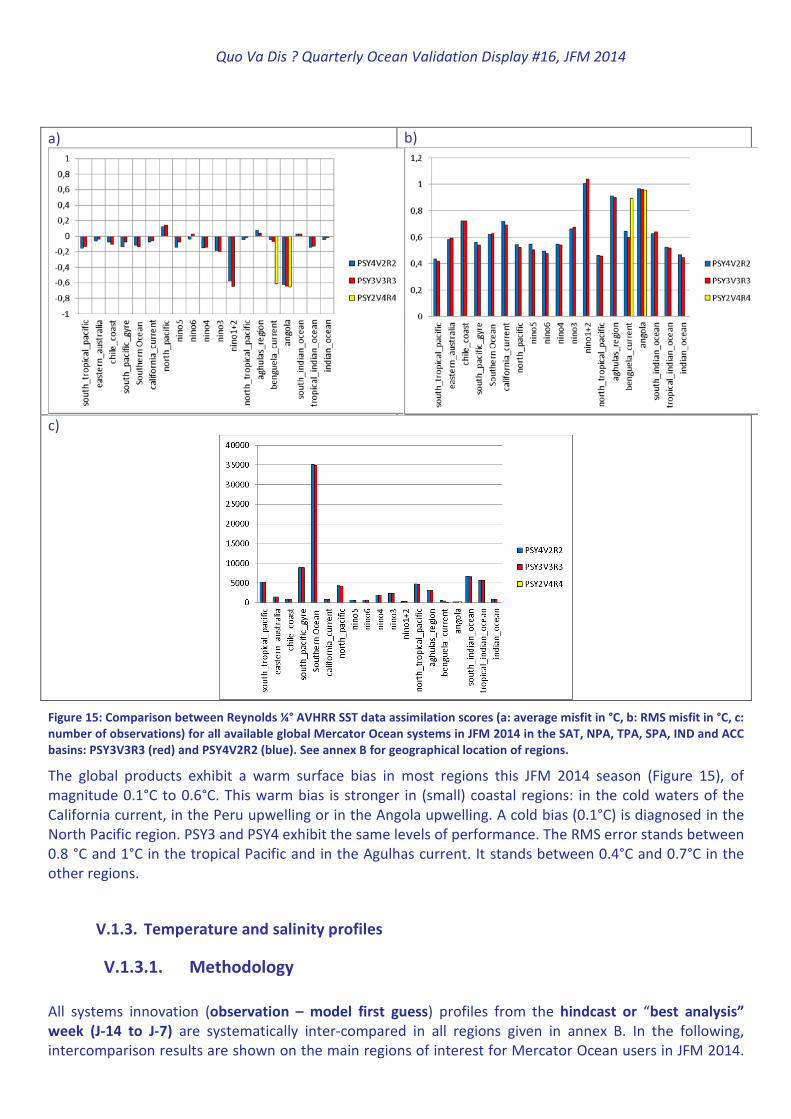
Figure 15: Comparison between Reynolds ¼° AVHRR SST data assimilation scores (a: average misfit in °C, b: RMS misfit in °C, c:
number of observations) for all available global Mercator Ocean systems in JFM 2014 in the SAT, NPA, TPA, SPA, IND and ACC
basins: PSY3V3R3 (red) and PSY4V2R2 (blue). See annex B for geographical location of regions.
The global products exhibit a warm surface bias in most regions this JFM 2014 season (Figure 15), of
magnitude 0.1°C to 0.6°C. This warm bias is stronger in (small) coastal regions: in the cold waters of the
California current, in the Peru upwelling or in the Angola upwelling. A cold bias (0.1°C) is diagnosed in the
North Pacific region. PSY3 and PSY4 exhibit the same levels of performance. The RMS error stands between
0.8 °C and 1°C in the tropical Pacific and in the Agulhas current. It stands between 0.4°C and 0.7°C in the
other regions.
V.1.3. Temperature and salinity profiles
V.1.3.1. Methodology
All systems innovation (observation – model first guess) profiles from the hindcast or “best analysis”
week (J-14 to J-7) are systematically inter-compared in all regions given in annex B. In the following,
intercomparison results are shown on the main regions of interest for Mercator Ocean users in JFM 2014.
Quo Va Dis ? Quarterly Ocean Validation Display #16, JFM 2014
Some more regions are shown when interesting differences take place, or when the regional statistics
illustrate the large scale behaviour of the systems.
V.1.3.1.1. Basin scale statistics (GODAE metrics)
a)
b)
c)
d)

Quo Va Dis ? Quarterly Ocean Validation Display #16, JFM 2014
e)
f)
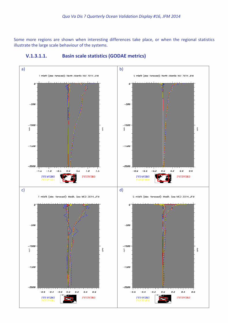
Figure 16: Profiles of JFM 2014 innovations of temperature (°C, left column) and salinity (psu, right column), mean (solid line)
and RMS (dashed line) for PSY3V3R3 (red), PSY2V4R4 (yellow) and PSY4V1R3 (blue) in the North Atlantic NAT (a and b),
Mediterranean Sea MED (c and d) and Arctic Ocean ARC (e an fl, the region starts of north of 67°N). Basin masks are applied
to keep only the main basin of interest (no Mediterranean in the Altantic NAT, no Black Sea in the Mediterranean MED, etc…).
On average over the North Atlantic, PSY4 displays a warm bias from 50 m to 500 m that is not present in
PSY3 (Figure 16). In the meantime, a slight salty bias of around 0.05 psu is diagnosed in all systems near
100m. On average over the Mediterranean Sea, PSY4 displays a noisy temperature error profile, with an
average warm bias between 0 m and 500 m, and a cold bias between 500 and 800m. PSY2 displays the best
performance in the Mediterranean, while PSY3 has a cold and fresh bias near 100m and a salty surface
bias. In the Arctic, a cold bias is diagnosed in both PSY3 and PSY4 between 400 and 900m. A salty bias of
around 0.2 psu can be found at the surface and decreases with depth until 100m.
On average over the Tropical Atlantic basin PSY4 exhibits warm (0.3°C) and salty (around 0.05 psu) biases
in the 50-300m layer (Figure 17). No significant temperature or salinity biases appear underneath the
surface layer. PSY3 (closely followed by PSY2) exhibits the best performance in this region.
PSY3 is less biased than PSY4 as well in the South Atlantic Basin, where PSY4 is too warm in the 50-800 m
layer, while PSY3 and PSY4 are both slightly too fresh near the surface. In the Indian Ocean PSY3 exhibits a
cold bias (0.2°C near 100m and then 0.1 °C between 150 and 500m). PSY4 also exhibits a cold bias in the
surface layer (0-100m) and displays a warm bias in the 100-200m layer. The surface layer from 0 to 200 m
is slightly too salty in both systems (0.02 psu).

Quo Va Dis ? Quarterly Ocean Validation Display #16, JFM 2014
a)
b)
c)
d)

Quo Va Dis ? Quarterly Ocean Validation Display #16, JFM 2014
e)
f)
Figure 17: As Figure 16 in the Tropical Atlantic TAT (a and b), South Atlantic SAT (c and d) and Indian IND (e and f) basins.
On average over the Pacific Ocean (Figure 18), PSY4 is warmer (0.1 to 0.2 °C) than the observations (and
than PSY3) from the surface to 500 m. On the contrary PSY3 exhibits a cold bias of around 0.1°C in the
same layer in the Tropical Pacific.

Quo Va Dis ? Quarterly Ocean Validation Display #16, JFM 2014
a)
b)
c)
d)

Quo Va Dis ? Quarterly Ocean Validation Display #16, JFM 2014
e)
f)
Figure 18: As Figure 16 in the North Pacific NPA (a and b), Tropical Pacific TPA (c and d) and South Pacific SPA (e and f).
For both PSY3 and PSY4 the salinity bias vertical structure is the same, and its amplitude is small (less than
0.05 psu, with a maximum fresh bias at the surface). A salty bias is diagnosed near 100 m over the whole
Pacific Ocean, and a second salty bias appears near 200m in the Tropical and South Pacific. The
temperature and salinity RMS errors of PSY3 and PSY4 are identical while the bias is stronger in PSY4 which
means that the variability is probably better represented in PSY4 than in PSY3.
In the Southern Ocean in Figure 19, a warm temperature bias is observed again in PSY4 (up to 0.2 °C near
200m) while PSY3 is nearly unbiased, except for a cold (0.1 °C) and salty (0.03 psu) bias maximum near the
surface.

Quo Va Dis ? Quarterly Ocean Validation Display #16, JFM 2014
a)
b)
Figure 19: As Figure 16 in the ACC Southern Ocean basin (from 35°S).
V.1.3.1.2. Atlantic sub-regions
a)
b)

Quo Va Dis ? Quarterly Ocean Validation Display #16, JFM 2014
c)
d)
Figure 20: As Figure 16 in the North East Atlantic (IBI) and the North Madeira XBT regions.
The previous general comments apply also in smaller regions of the North East Atlantic Ocean, as shown in
Figure 20. The signature of the Mediterranean waters is clear in the T and S RMS error for all systems
(Figure 20 c and d). This quarter is characterized by the warm bias in both high resolution systems PSY2
and PSY4 in the 50-500 m layer. PSY3 on the contrary exhibits a cold bias in the same layer. Near 50m all
systems display a cold bias, while they all exhibit a warm bias near 1000m. PSY2 and PSY3 (in the North
Madeira region) are less biased than PSY4 this JFM season. In the Mediterranean water outflow the RMS
error of PSY4 is higher than that of the other systems.
In sub-regions of the Tropical Atlantic and in the Gulf Stream (Figure 21), the vertical structure of the biases
is more complex. It reflects the underestimation of the upwelling in the Dakar region, and the errors in the
vertical structure of the currents. In the Gulf of Mexico the systems are too cold near 150, and then
warmer than observations between 200 and 800m. In this region, PSY4 is less biased than PSY2 and PSY3.
In the Gulf Stream, all systems are too warm (1°C) in the 0-500m layer. Underneath PSY3 is too warm and
salty until 1500m, while PSY4 is too cold from 800 to 1500m.

Quo Va Dis ? Quarterly Ocean Validation Display #16, JFM 2014
a)
b)
Figure 21: As Figure 16 in the Dakar region.
a)
b)

Quo Va Dis ? Quarterly Ocean Validation Display #16, JFM 2014
c)
d)
e)
f)
Figure 22: As Figure 16 in the Ascension tide (a and b), the Gulf of Mexico (c and d) and the Gulf Stream 1 regions (e and f)
However, one must keep in mind that the smallest sub-regions contain only a few data per assimilation
cycle and that in this case the statistics may not be representative of the whole period, see for instance in
Figure 23.

Quo Va Dis ? Quarterly Ocean Validation Display #16, JFM 2014
a)
b)
Figure 23:number of observations of T (a) and S (b) assimilated in PSY4V2R2 in the Gulf Stream 1 region during the JFM 2014
quarter.
V.1.3.1.3. Mediterranean Sea sub-regions
a)
b)

Quo Va Dis ? Quarterly Ocean Validation Display #16, JFM 2014
c)
d)
e)
f)

Quo Va Dis ? Quarterly Ocean Validation Display #16, JFM 2014
g)
h)
Figure 24: As Figure 16 in the Algerian (a and b), the gulf of Lion (c and d), the Ionian (e and f) and the Mersa Matruh (g and h)
regions.
Figure 24 shows the T and S error profiles in sub-regions of the Mediterranean Sea. Biases are more
pronounced this season in the Eastern part of the basin, with a warm and salty bias in the 0-100m layer
and between 100 and 800m. In the central Ionian region, a surface salty bias is present between 0 and
100m in PSY4 while it is fresh in the two other systems.
V.1.3.1.4. Indian Ocean sub-regions
Quo Va Dis ? Quarterly Ocean Validation Display #16, JFM 2014
a)
b)
c)
d)
Quo Va Dis ? Quarterly Ocean Validation Display #16, JFM 2014
e)
f)
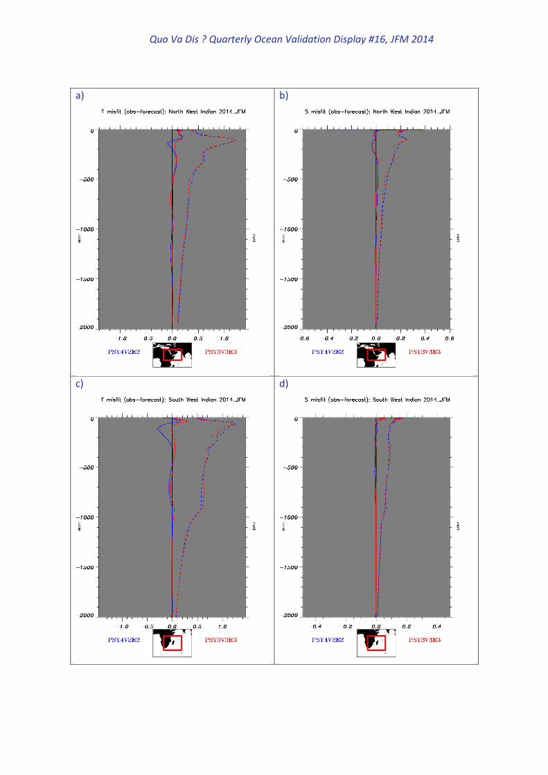
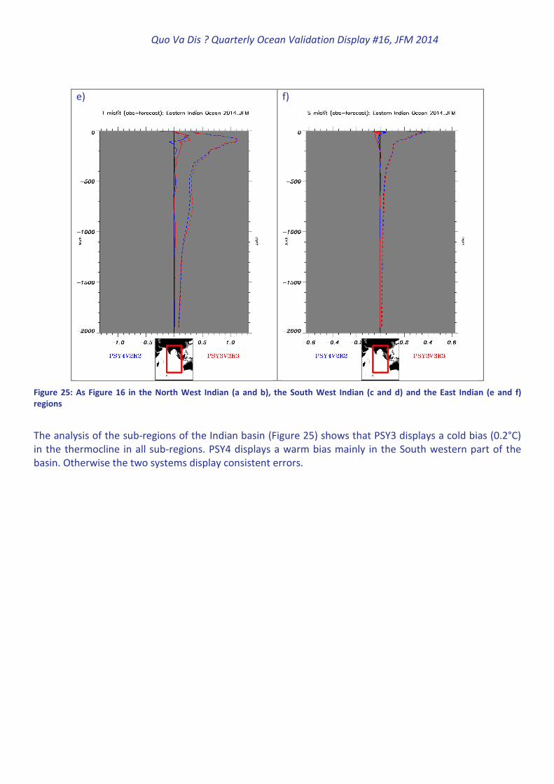
Figure 25: As Figure 16 in the North West Indian (a and b), the South West Indian (c and d) and the East Indian (e and f)
regions
The analysis of the sub-regions of the Indian basin (Figure 25) shows that PSY3 displays a cold bias (0.2°C)
in the thermocline in all sub-regions. PSY4 displays a warm bias mainly in the South western part of the
basin. Otherwise the two systems display consistent errors.

Quo Va Dis ? Quarterly Ocean Validation Display #16, JFM 2014
SUMMARY: Starting in April 2013, the PSY2, PSY3 and PSY4 systems converge in terms of model version
and parameterizations. The data assimilation method and tunings are the same, and so do the data sets
assimilated by the three systems. In consequence, the three Mercator Ocean systems display consistent
data assimilation statistics for the quarter JFM 2014. The systems are close to the observations, and
misfits lie within the prescribed error (most of the time misfit in T is less than 0.1 °C, misfit in S less then
0.05 psu, misfit in SLA less than 7 cm). The average and RMS errors are larger in regions of high spatial
and/or temporal variability (thermocline, regions of high mesoscale activity, upwelling, fronts, etc…). PSY4
displays a warm bias in the 0-800m layer that is not present in PSY2 and PSY3. This difference between
PSY4 and the other systems is mainly due to the initialization of the system, which took place in October
2012 (in October 2009 for PSY2 and PSY3). The analysis of the GLORYS2V3 reanalysis has shown that the
first cycles of SLA data assimilation induce a large warming of the ocean in the 0-800m layer that the in situ
observations have to correct. The SEEK and the 3D-var bias correction need at least a one year period to
correct this bias, which is then propagated to the deep layers (under 1000m) within 5 to 10 years, if no
correction is applied. Thus PSY4’s warm bias should start decreasing in 2014, while the drift of
temperature and salinity at depth has to be controlled in PSY2 and PSY3. Consequently PSY4 also displays
low biases in SLA concurrent with warm biases in SST. Coastal regions are weakly constrained in all
systems, and consistent biases appear in SLA and SST (warm and high, or cold and low). There are still
many uncertainties in the MDT, mainly near the coasts and in the Polar Regions. The systems do not use
the SLA misfit information in coastal regions, but problems can appear in open ocean regions where there
are still errors in the MDT. Seasonal biases have been reduced with respect to previous versions of the
systems, thanks to the use of a procedure to avoid the damping of SST increments via the bulk forcing
function. A warm bias is diagnosed in SST this quarter. There is still too much mixing in the surface layer
inducing a cold bias in the surface layer (0-50 m) and warm bias in subsurface (50-150 m). This bias is
intensifying with the summer stratification and the winter mixing episodes reduce the bias. This bias is thus
reduced this JFM 2014 season in the North Atlantic, but the vertical structure of the bias is still diagnosed
for instance in the North Eastern part of the basin. The bias correction is not as efficient on reducing
seasonal biases as it is on reducing long term systematic biases. No precipitation correction is applied in
the systems, and uncertainties (overestimation) of the convective precipitations induce large fresh biases
in the tropical oceans (for instance this season in the Tropical Atlantic).

Quo Va Dis ? Quarterly Ocean Validation Display #16, JFM 2014
V.2. Accuracy of the daily average products with respect to observations
V.2.1. T/S profiles observations
V.2.1.1. Global statistics for JFM 2014
a)
b)
c)
d)
e)
f)
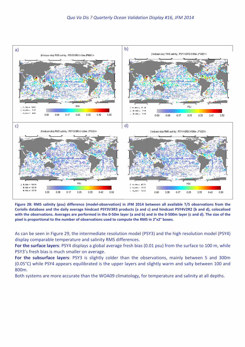
Figure 26: Average difference MODEL-OBSERVATION of temperature (a, c, and e, in °C) and salinity (b, d, and f, in psu) in JFM
2014 between the daily average hindcast PSY4V2R2 (a and b), PSY3V3R3 (c and d) and PSY2V4R4 (e and f) hindcast products
and all available T/S observations from the Coriolis database. The Mercator hindcast products are taken at the time and
location of the observations. Averages are performed in the 0-50m layer. The size of the pixel is proportional to the number
of observations used to compute the RMS in 2°x2° boxes.

Quo Va Dis ? Quarterly Ocean Validation Display #16, JFM 2014
a) b)
c) d)
Figure 27: RMS temperature (°C) difference (model-observation) in JFM 2014 between all available T/S observations from the
Coriolis database and the daily average hindcast PSY3V3R3 products on the left and hindcast PSY4V2R2 on the right column
colocalised with the observations. Averages are performed in the 0-50m layer (a and b) and in the 0-500m layer (c and d). The
size of the pixel is proportional to the number of observations used to compute the RMS in 2°x2° boxes.
Consistently with the data assimilation statistics the three systems PSY3, PSY4 and PSY2 are slightly colder
(~0.1°C) than the observations at the global scale in the surface layer (0-50m) as can be seen in Figure 26,
especially in Tropical Pacific and Atlantic basins. Fresh biases also appear in the tropics, linked with
overestimated convective precipitations in the ECMWF analyses, and also to the climatological runoffs that
are prescribed. This quarter the bias is significantly stronger in PSY4 than in PSY2 or PSY3. A fresh bias also
appears in PSY4 in the California current.
As can be seen in Figure 27, in both PSY3 and PSY4 temperature errors in the 0-500m layer have similar
amplitude and spatial patterns, and stand between 0.5 and 1°C in most regions of the globe. RMS errors in
the tropical thermocline can reach 1°C. Regions of high mesoscale activity (Kuroshio, Gulf Stream, Agulhas
current) and regions of upwelling in the tropical Atlantic and Tropical Pacific display higher errors (up to
3°C).
The salinity RMS errors (Figure 28) are usually less than 0.2 psu but can reach higher values in regions of
high runoff (Amazon, Sea Ice limit) or precipitations (ITCZ, SPCZ, Gulf of Bengal), and in regions of high
mesoscale variability. RMS errors of around 0.2 psu in the Tropics in the 0-50m layer correspond to the
fresh bias linked with overestimated precipitation.
Quo Va Dis ? Quarterly Ocean Validation Display #16, JFM 2014
a)
b)
c) d)
Figure 28: RMS salinity (psu) difference (model-observation) in JFM 2014 between all available T/S observations from the
Coriolis database and the daily average hindcast PSY3V3R3 products (a and c) and hindcast PSY4V2R2 (b and d), colocalised
with the observations. Averages are performed in the 0-50m layer (a and b) and in the 0-500m layer (c and d). The size of the
pixel is proportional to the number of observations used to compute the RMS in 2°x2° boxes.
As can be seen in Figure 29, the intermediate resolution model (PSY3) and the high resolution model (PSY4)
display comparable temperature and salinity RMS differences.
For the surface layers: PSY4 displays a global average fresh bias (0.01 psu) from the surface to 100 m, while
PSY3’s fresh bias is much smaller on average.
For the subsurface layers: PSY3 is slightly colder than the observations, mainly between 5 and 300m
(0.05°C) while PSY4 appears equilibrated is the upper layers and slightly warm and salty between 100 and
800m.
Both systems are more accurate than the WOA09 climatology, for temperature and salinity at all depths.

Quo Va Dis ? Quarterly Ocean Validation Display #16, JFM 2014
a)
b)
c)
d)
Figure 29 : JFM 2014 global statistics of temperature (°C, a and c) and salinity (psu, b and d) averaged in 6 consecutive layers
from 0 to 5000m. RMS difference (a and b) and mean difference (observation-model, c and d) between all available T/S
observations from the CORIOLIS database and the daily average hindcast products PSY3V3R3 (red), PSY4V2R2 (blue) and
WOA09 climatology (grey) colocalised with the observations. NB: average on model levels is performed as an intermediate
step which reduces the artefacts of inhomogeneous density of observations on the vertical.

Quo Va Dis ? Quarterly Ocean Validation Display #16, JFM 2014
a)
b)
c)
d)
Figure 30: RMS difference (model-observation) of temperature (a and b, °C) and salinity (c and d, psu) in JFM 2014 between
all available T/S observations from the Coriolis database and the daily average PSY2V4R4 hindcast products colocalised with
the observations in the 0-50m layer (a and c) and 0-500m layer (b and d)
The general performance of PSY2 (departures from observations in the 0-500m layer) is less than 0.3°C and
0.05 psu in many regions of the Atlantic and Mediterranean (Figure 30). The strongest departures from
temperature and salinity observations are mainly located in the Gulf Stream and the tropical Atlantic. Near
surface salinity biases appear in the Alboran Sea, the Gulf of Guinea, the Caribbean Sea, the Labrador Sea
and the Gulf of Mexico (see also Figure 26). In the tropical Atlantic biases concentrate in the 0-50m layer
(cold and fresh bias). This is consistent with the bias correction not being at work in the mixed layer.

Quo Va Dis ? Quarterly Ocean Validation Display #16, JFM 2014
V.2.1.2. Water masses diagnostics
a) b) c)
d) e) f)
g) h) i)

Quo Va Dis ? Quarterly Ocean Validation Display #16, JFM 2014
j) k) l)
Figure 31: Water masses (Theta, S) diagrams in JFM 2014 in the Bay of Biscay (a to c), Gulf of Lion (d to f), Irminger Sea (g to i)
and Gulf of Cadiz (j to l), comparison between PSY3V3R3 (a, d, g, j), PSY4V2R2 (b, e, h, k) and PSY2V4R4 (c, f, I, and l) in AMJ
2013. PSY2, PSY3 and PSY4: yellow dots; Levitus WOA09 climatology: red dots; in situ observations: blue dots.
In Figure 31 the daily products (analyses) are collocated with the T/S profiles in order to draw “T, S”
diagrams. The water masses characteristics of the three systems are nearly similar, PSY4 being locally
slightly better than PSY3 and PSY2 (Mediterranean waters)
In the Bay of Biscay the Eastern North Atlantic Central Water, Mediterranean and Labrador Sea Water can
be identified on the diagram.
- Between 11°C and 15°C, 35 and 36 psu, warm and relatively salty Eastern North Atlantic Central
Water gets mixed with the shelf water masses. The saltiest ENACW waters are well captured by by
the three systems during this JFM 2014 season.
- The Mediterranean Waters are characterized by high salinities (Salinities near 36 psu) and relatively
high temperatures (Temperatures near 10°C). PSY4 better captures the highest salinities than PSY3
and PSY2 for the main profiles. A few profiles appear much more saltier in the Mercator systems
than the in situ data.
- The Labrador Sea waters appear between 4°C and 7°C, 35.0 and 35.5 psu and are well represented
by the three system, especially for PSY4.
In the Gulf of Lion:
- The Levantine Intermediate Water (salinity maximum near 38.6 psu and 13.3°C) is too cold and
little fresh and compact in all systems this JFM 2014 season.
- The water mass detected near 38.5 psu and 13-13.3°C may correspond to measurements on the
shelves made by research vessels.
In the Irminger Sea:
- The Irminger Sea Water (≈ 3°C and 35 psu) and the North Atlantic water (at the surface) are well
represented by the systems.
- The Labrador Sea Waters are too salty in all systems.
- Waters colder than 3°C and ≈ 34.9 psu (Iceland Scotland Overflow waters) are presents in all
systems but seem too fresh.
In the Gulf of Cadiz:
- The Mediterranean outflow waters (T around 10°C) are well represented but appears too fresh in
the three systems. The high resolution systems (PSY2 and PSY4) better capture the spread of
temperature and salinity at depth as well as at the surface (Atlantic Surface waters).

Quo Va Dis ? Quarterly Ocean Validation Display #16, JFM 2014
In the western tropical Atlantic, all the systems capture the salinity minimum of the Antarctic
Intermediate Waters (AIW). The spread of temperature and salinity at surface and sub-surface is well
represented too.
In the eastern tropical Atlantic the three systems represent well the water masses. South Atlantic PSY2
(and to a lesser extent PSY4) displays fresh waters near the surface that are not present in the
observations.
a) b) c)
d) e) f)
Figure 32 : Water masses (T, S) diagrams in the Western Tropical Atlantic (a to c) and in the Eastern Tropical Atlantic (d to f) in
JFM 2014: for PSY3V3R3 (a, d); PSY4V2R2 (b, e); and PSY2V4R4 (c, f). PSY2, PSY3 and PSY4: yellow dots; Levitus WOA09
climatology; red dots, in situ observations: blue dots.
In the Agulhas current (Figure 33) PSY3 and PSY4 give a realistic description of water masses. The central
and surface waters characteristics are slightly more realistic in PSY4 than in PSY3. In the Kuroshio region
the North Pacific Intermediate waters (NPIW) are too salty for the two global systems. At the surface in the
highly energetic regions of the Agulhas and of the Gulf Stream, the water masses characteristics display a
wider spread in the high resolution 1/12° than in the ¼°, which is more consistent with T and S
observations. In the Gulf Stream region, PSY4 is closer to the observations than PSY3 especially in the
North Atlantic Central Waters (NACW) where PSY3 is too fresh. The saltiest waters near the surface (North
Atlantic Subtropical Waters, NASW) are only captured by PSY4.

Quo Va Dis ? Quarterly Ocean Validation Display #16, JFM 2014
a)
b)
c)
d)

Quo Va Dis ? Quarterly Ocean Validation Display #16, JFM 2014
e)
f)
Figure 33: Water masses (T, S) diagrams in South Africa (a and b), Kuroshio (c and d), and Gulf Stream region (e and f): for
PSY3V3R1 (a, c and e); PSY4V1R3 (b, d and f) in JFM 2014. PSY3 and PSY4: yellow dots; Levitus WOA09 climatology: red dots;
in situ observations: blue dots.
V.2.2. SST Comparisons
Quarterly average SST differences with OSTIA analyses show that the systems’ SST is very close to OSTIA,
with difference values staying below the observation error of 0.5 °C on average. High RMS difference
values (Figure 34) are encountered in high spatial and temporal variability regions such as the Gulf Stream
or the Kuroshio. The error is also high (more than 2°C locally) in marginal seas of the Antarctic and Arctic
Ocean where the sea ice limit increases the SST errors and the SST contrasts (especially with the Antarctic
ice extend record this year). Small features in the RMS difference appear in PSY3 that are not found in the
higher resolution systems PSY4 and PSY2 (for instance this quarter in the Baltic Sea or in the Mauritanian
upwelling).
a)
b)

Quo Va Dis ? Quarterly Ocean Validation Display #16, JFM 2014
c)
Figure 34 : RMS temperature (°C) differences between OSTIA daily analyses and PSY3V3R3 daily analyses (a); between OSTIA
and PSY4V2R2 (b), between OSTIA and PSY2V4R4 (c) in JFM 2014. The Mercator Océan analyses are colocalised with the
satellite observations analyses.
The systems’ tropical oceans are warmer than OSTIA (Figure 35), as do the high latitudes (especially in the
ACC this austral winter). The Pacific subtropical and the Indian Ocean are colder than OSTIA on average, as
do some closed or semi-enclosed seas: the Gulf of Mexico; China Sea and along the Peru-Chili Coast.
a)
b)
c)
Figure 35: Mean SST (°C) daily differences in JFM 2014 between OSTIA daily analyses and PSY3V3R3 daily analyses (a),
between OSTIA and PSY4V2R2 (b) and between OSTIA and PSY2V4R4 daily analyses (c).

Quo Va Dis ? Quarterly Ocean Validation Display #16, JFM 2014
V.2.3. Drifting buoys velocity measurements
Recent studies (Law Chune, 20123 , Drévillon et al, 2012
4) - in the context of Search-And-Rescue and drift
applications – focus on the need for accurate surface currents in ocean forecasting systems. In situ currents
are not yet assimilated in the Mercator Ocean operational systems, as this innovation requires a better
characterization of the surface currents biases.
The comparison of Mercator analyses and forecast with AOML network drifters’ velocities combine two
methods based on Eulerian and Lagrangian approaches.
V.2.3.1. Eulerian Quality control
a) b)
c) d)
3 Law Chune, 2012 : Apport de l’océanographie opérationnelle à l’amélioration de la prévision de la dérive océanique
dans le cadre d’opérations de recherche et de sauvetage en mer et de lutte contre les pollutions marines
4 Drévillon et al, 2012 : A Strategy for producing refined currents in the Equatorial Atlantic in the context of the
search of the AF447 wreckage (Ocean Dynamics, Nov. 2012)

Quo Va Dis ? Quarterly Ocean Validation Display #16, JFM 2014
e)
f)
Figure 36: Near surface (15m) zonal current (m/s) comparison between the Mercator systems analyses and observed
velocities from drifters. In the left column: velocities collocated with drifter positions in JFM 2014 for PSY3V3R3 (a), PSY4V2R2
(c) and PSY2V4R4 (e). In the right column, zonal current from drifters in JFM 2014 (b) at global scale, AOML drifter climatology
for JFM with new drogue correction from Lumpkin & al, in preparation (d) and observed zonal current in JFM 2014 (f) over
PSY2’s domain.
a)
b)
c)
d)

Quo Va Dis ? Quarterly Ocean Validation Display #16, JFM 2014
e)
f)
Figure 37 : In JFM 2014, comparison of the mean relative velocity error between in situ AOML drifters and model data (a, c
and e) and mean zonal velocity bias between in situ AOML drifters with Mercator Océan correction (see text) and model data
(b, d and f). a and b: PSY3V3R3, c and d: PSY4V2R3, e and f: PSY2V4R2. NB: zoom at 500% in order to see the arrows.
The fact that velocities estimated by the drifters happen to be biased towards high velocities is taken into
account, applying slippage and windage corrections (cf QuO Va Dis? #5 and Annex C). Once this so called
“Mercator Océan” correction is applied to the drifter observations, the zonal velocity of the model (Figure
36 and Figure 37) at 15 m depth and the meridional velocity (not shown) is more consistent with the
observations for the JFM 2014 period.
On average over long periods, the usual behaviour compared to drifters’ velocities is that the systems
underestimate the surface velocity in the mid-latitudes. All systems overestimate the Equatorial currents
and the southern part of the North Brazil Current (NBC).
For all systems the largest direction errors are local (not shown) and generally correspond to ill positioned
strong current structures in high variability regions (Gulf Stream, Kurioshio, North Brazil Current, Zapiola
eddy, Agulhas current, Florida current, East African Coast current, Equatorial Pacific Countercurrent).
The differences between the systems mainly appear in the North Atlantic and North Pacific Oceans on
Figure 37, in the relative error. In these regions PSY3 underestimates on average the eastward currents,
which is a bit less pronounced in the high resolution systems PSY4 and PSY2. On the contrary the systems
overestimate the equatorial westward currents on average, and this bias is less pronounced in PSY3 than in
PSY4. 50% of the ocean current feedbacks on the wind stress in PSY2 and PSY3, which slows the surface
currents with respect to PSY4.
V.2.3.2. Lagrangian Quality control
The aim of the Lagrangian approach is to compare the observed buoy trajectory with virtual trajectories
obtained with hindcast velocities, starting from the same observed initial location. The virtual trajectories
are computed with the ARIANE software5 (see annex II.2). The metric shown here (Figure 38) is the
distance between the trajectories after 1, 3 and 5 days, displayed at each trajectory initial point.
5 http://stockage.univ-brest.fr/~grima/Ariane/

Quo Va Dis ? Quarterly Ocean Validation Display #16, JFM 2014
a)
b)
c)
d)
e)
f)
Figure 38: In JFM 2014, comparison of the mean distance error in 1°x1° boxes after a 1-day drift (a and b), after a 3-days drift
(c and d), and after a 5-days drift (e and f).between AOML drifters’ trajectories and PSY3V3R3 trajectories (a, c, and e) and
between AOML drifters’ trajectories and PSY4V2R2 (b,d, and f).
Few differences appear between the systems and most of the high velocity biases that are diagnosed in
Figure 37 imply a large distance error (120 to 180km) after a few days drift in Figure 38. For instance in the
Pacific ocean, both PSY3 and PSY4 produce an error larger than 100km after only a 1-day drift near the
North Coast of Papua New Guinea.
In the subtropical gyres and in the North Pacific, which are less turbulent regions, the errors rarely exceed
30 km after 5 days.

Quo Va Dis ? Quarterly Ocean Validation Display #16, JFM 2014
Figure 39:Cumulative Distribution Functions of the distance error (km, on the left) and the direction error (degrees, on the
right panel) after 1 day (blue), 3 days (green) and 5 days (red), between PSY4V1R3 forecast trajectories and actual drifters
trajectories.
Over the whole domain on a long period, cumulative distribution functions (Figure 39) show that in 80% of
cases, PSY3 and PSY4 modelled drifters move away from the real drifters less than : 30km after 1 day,
70km after 3 days, and 100km after 5 days. As explained before, the remaining 20% generally correspond
to ill positioned strong current structures in high variability regions. PSY4 currents seem to induce slightly
more errors than PSY3 currents essentially for errors below 10-15 km. This is probably related to the high
mesoscale activity of the global high resolution model. This may not be systematic at the regional scale
(under investigation).
V.2.4. Sea ice concentration
a) b) c)

Quo Va Dis ? Quarterly Ocean Validation Display #16, JFM 2014
d)
e)
f)
Figure 40: Arctic (a to c) and Antarctic (d to f) JFM 2014 Sea ice cover fraction in PSY3V3R3 (a and d), in CERSAT observations
(b and e) and difference PSY3 – CERSAT (c and f).
On average over the JFM 2014 period, including the sea ice minimum of September, strong discrepancies
with observed sea ice concentration appear in the centre of the Arctic in PSY3 and PSY4 (Figure 40 and
Figure 41) as sea ice observations are not yet assimilated by the systems. Both PSY3 and PSY4 are melting
too much ice in summer, although differences are smaller in PSY4. The other small discrepancies that can
be distinguished inside the sea ice pack will not be considered as significant as the sea ice concentration
observations over 95% are not reliable. Differences with the observations remain significant in the
marginal seas, for instance the sea ice melts too much in the Denmark Strait.
Model studies show that the overestimation in the Canadian Archipelago is first due to badly resolved sea
ice circulation. The overestimation in the eastern part of the Labrador Sea is due to a weak extent of the
West Greenland Current; similar behaviour in the East Greenland Current.
In the Antarctic the winter sea ice concentration is overestimated on average by both PSY3 and PSY4, for
instance in the Weddell Sea. On the contrary it is underestimated along the sea ice edge.
a) b) c)

Quo Va Dis ? Quarterly Ocean Validation Display #16, JFM 2014
d)
e)
f)
Figure 41: Arctic (a to c) and Antarctic (d to f) JFM 2014 Sea ice cover fraction in PSY4V2R2 (a and d), in CERSAT observations
(b and e) and difference PSY4 – CERSAT (c and f).
Figure 42 illustrates the fact that sea ice cover in JFM 2014 is less than the past years climatology,
especially in the Nansen Basin (see also section IV).
a)
b)

Quo Va Dis ? Quarterly Ocean Validation Display #16, JFM 2014
c)
d)
Figure 42: JFM 2014 Arctic sea ice extent in PSY4V2R2 with overimposed climatological AMJ 1992-2010 sea ice fraction
(magenta line, > 15% ice concentration) (a) and NSIDC map of the sea ice extent in the Arctic for March 2014 in comparison
with a 1979-2000 median extend (b).
V.2.5. Closer to the coast with the IBI36V2 system: multiple comparisons
V.2.5.1. Comparisons with SST from CMS
The bias, RMS error and correlation calculated from comparisons with SST measured by satellite in JFM
2014 (Météo-France CMS high resolution SST at 0.02°) are displayed in Figure 43. The biases are reduced in
winter with respect to the summer and autumn region. The cold bias is persisting in the North Sea. A warm
bias is present along the south Moroccan coast and Canary Islands, and in a large area west of the Iberian
Peninsula between 35°N and 50°N. This last warm bias was not present in JFM 2013 and 2012 (not shown).
In the Mediterranean Sea a warm bias can be noticed in the south-west corner of Spain. Low correlations
(<0.4) are observed this season in the Bay of Biscay, in the Gulf of Lion and in the North Sea, despite the
sample size which is significant. This is also the case in PSY2 (IBI’s parent system) and in PSY4. Thanks to
data assimilation, the bias and RMS with respect to CMS observations is most of the time smaller in PSY2
than in IBI. In PSY4 a warm anomaly appears off the Portuguese coast, which is partly due to a spurious
warm core eddy which forms in this area in February, and which PSY4 does not manage to correct (ref
etude).
Note that the number of observations over the shelf and Mediterranean Sea is very good for JFM 2014
compared to previous years.

Quo Va Dis ? Quarterly Ocean Validation Display #16, JFM 2014
a)
b)
c)
j)
d)
e)
f)
g)
h)
i)
Figure 43 : Mean bias (model-observation) (a), RMS error (b), correlation (c) between IBI36V2 and analysed L3 SST from
Météo-France CMS for the JFM 2014 quarter. Same diagnostics for PSY2V4R4 (d,e,f) and PSY4V2R2 (g,h,i). Number of Météo-
France CMS observations for the JFM 2014 quarter (j).
V.2.5.2. Comparisons with in situ data from EN3/ENSEMBLE for JFM 2014

Quo Va Dis ? Quarterly Ocean Validation Display #16, JFM 2014
Averaged temperature profiles (Figure 44) show that the model is close to the observations and to the
models PSY2V4R2 and PSY2V4R4 in the whole water column (rms lower or equal to 0.5°C). In the Bay of
Biscay, the strongest mean and RMS error are observed between 800 and 1600 m depth: the
Mediterranean waters are slightly too warm. Deeper than 1200 m, PSY2V4R4 is closer to the observations
than PSY2V4R2. Between 10 and 30 m depth, IBI36V2 is slightly closer to the observations than the PSY
systems.
a) Temperature, 0-200 m
b) Temperature, 0-2000 m
c) Temperature, 0-200 m
d) Temperature, 0-2000 m
Figure 44 : Over the whole IBI36V2 domain (a and b) and over the Bay of Biscay (c and d): mean “IBI36V2 - observation”
temperature (°C) bias (red) and RMS error (blue) in JFM 2014 (a and c), and mean profile from IBI36V2 (black), PSY2V4R4
(green) and from the observations (red) in JFM 2014 (b and d). In the lower right corner of each plot: position of the individual
profiles.
The maximum salinity bias and RMS error (Figure 45) occur near the surface. The model is too fresh near
the surface. Below 100 m depth, the bias is almost zero. The RMS error is strong at the surface and
Mediterranean Sea Water level (as for temperature). In the Bay of Biscay the Mediterranean waters are
too salty. PSY2V4R4 performs better than the other models.
Note: averaged profiles are discontinuous because the number of observations varies with depth.

Quo Va Dis ? Quarterly Ocean Validation Display #16, JFM 2014
a) Salinity, 0-200 m
b) Salinity, 0-2000 m
c) Salinity, 0-200 m
d) Salinity, 0-2000 m
Figure 45: Over the whole IBI36V2 domain (a and b) and over the Bay of Biscay (c and d): mean “IBI36V2 - observation”
salinity (psu) bias (red) and RMS error (blue) in JFM 2014 (a and c), and mean profile from IBI36V2 (black), PSY2V4R4 (green)
and from the observations (red) in JFM 2014 (b and d). In the lower right corner of each plot: position of the individual
profiles.
V.2.5.3. MLD Comparisons with in situ data
Figure 46 shows that the distribution of modeled mixed layer depths among the available profiles is
comparable to the observed distribution for both PSY2 and IBI over the whole IBI domain. Values of the
mixed layer depth between 10 m and 15 m occur too often in the systems compared with the observations
(especially for PSY2), suggesting the mixed layer is too shallow in the systems. On the contrary, values
between surface and 30 m are under-estimated by PSY2. In the Bay of Biscay IBI36 is closer to the
observations than PSY2. Both systems over-estimate values between 100 and 160 m, and between 400 and
600 m. In the Bay of Biscay and Channel, the MLD distribution of IBI36 is closer to the observations than
that of PSY2.

Quo Va Dis ? Quarterly Ocean Validation Display #16, JFM 2014
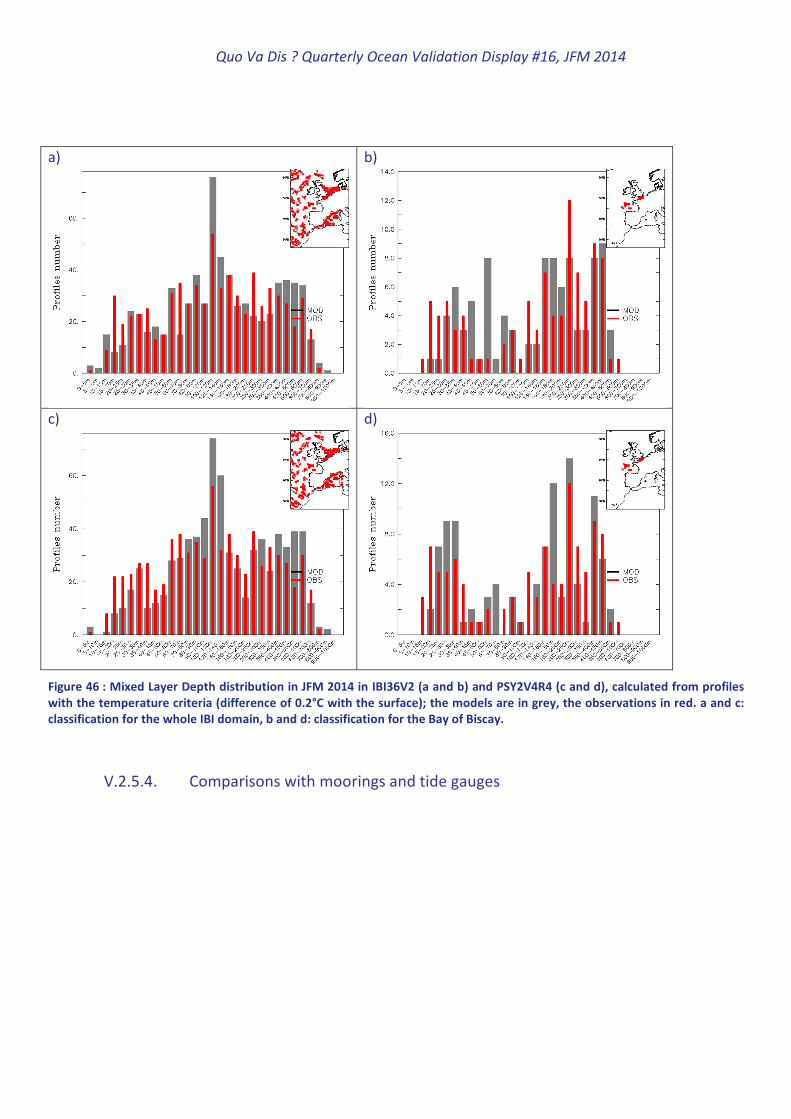
Quo Va Dis ? Quarterly Ocean Validation Display #16, JFM 2014
a)
b)
c)
d)
Figure 46 : Mixed Layer Depth distribution in JFM 2014 in IBI36V2 (a and b) and PSY2V4R4 (c and d), calculated from profiles
with the temperature criteria (difference of 0.2°C with the surface); the models are in grey, the observations in red. a and c:
classification for the whole IBI domain, b and d: classification for the Bay of Biscay.
V.2.5.4. Comparisons with moorings and tide gauges

Quo Va Dis ? Quarterly Ocean Validation Display #16, JFM 2014
a)
b)
Figure 47 : For IBI36V2: RMS error (a, in cm) and correlation (b) for the non-tidal Sea Surface Elevation at tide gauges in JFM
2014, for different regions and frequencies.
The RMS error of the residual (non tidal) elevation of sea surface (Figure 47) computed with harmonic
decomposition (Foreman 1977) and Loess low-pass filtering is between 4 and 16 cm. It is close to 5 cm in
the Canary Islands, Mediterranean Sea and Iberian Coast. The RMS decreases for some frequency bands,
and the smallest values occur in the 1-10-day band. The correlation is significant at all frequencies, and
reaches high values for periods generally lower than 30 days (at high frequencies).

Quo Va Dis ? Quarterly Ocean Validation Display #16, JFM 2014
a)
b)
c)
d)
e)
f)
g)
h)
i)
Figure 48 : For IBI36V2: Bias (observation-model) (a, d and g), RMS error (°C) (b, e and h) and correlation (c, f and i) of the Sea
Surface Temperature between IBI36 and moorings measurements in January (a to c), February (d to f) and March 2014 (g to i).

Quo Va Dis ? Quarterly Ocean Validation Display #16, JFM 2014
In Figure 48 (and Figure 49) we can see that the SST correlations between the coastal moorings and the IBI
model can vary a lot during the three months, depending of the period and the location. February is
characterized by the lowest correlation, in particular along the Spanish coast and in the Gulf of Lions. The
RMS values are generally lower than 0.5°C. The model temperature is generally higher than the
observations along the Spanish coast, and lower in the Channel and Gulf of Lions, consistently with the L3
SST biases of Figure 43.
Estaca de bares
Biscay
Les pierres noires
Sandettie lightship
Gulf of Lion
Figure 49: Surface temperature (°C) time series at a selection of moorings which locations are shown on the upper left panel
(no observation for Gulf of Lion).

Quo Va Dis ? Quarterly Ocean Validation Display #16, JFM 2014
V.2.6. Biogeochemistry validation: ocean colour maps
a) b)
c) d)
e) f)
Figure 50 : Chlorophyll-a concentration (mg/m3) in January (a and b), February (c and d) and March 2014 (e and f) for the
Mercator system BIOMER (a, c, and e) and Chlorophyll-a concentration from Globcolour (b, d and f).
As can be seen on Figure 50 the surface chlorophyll-a concentration is overestimated by BIOMER on
average over the globe. The production is especially overestimated in the northern hemisphere (Atlantic
and Pacific) North Pacific North and North Atlantic and slightly in the tropical band. The bloom observed in
the northern hemisphere subpolar gyre just started in March, when it already appears very strong in early

Quo Va Dis ? Quarterly Ocean Validation Display #16, JFM 2014
January in BIOMER. Some coastal regions or semi enclosed seas like the North and Baltic seas or the China
Seas do not display local enrichments that can be detected in the observations. On the contrary, BIOMER
displays unobserved enrichments in the upwelling of Peru and Benguela, as well as in regions of high
variability sugh as the Zapiola eddy or the Somali Gyre. Figure 54 shows the PDF of the Chl-a bias in North
Atlantic. The negative values between 0 and -1 mg/m3 correspond mainly to the high values of the bloom
in BIOMER not present in Globcolour dataset. The highest negative biases are observed in March.
a)
b)
c)
Figure 51 : Probability Density Function (PDF) of Chl-a bias in log scale (log10(obs)-log10(model)) in the North Atlantic (30-
70N; 80W:20E) for January (a), February (b) and March (c) 2014.
The discrepancies at the global scale appear in the RMS differences for the mean JFM 2014 season (Figure
52).
Figure 52 : RMS difference between BIOMER and Globcolour Chl-a concentrations (mg/m3) in JFM 2014.

Quo Va Dis ? Quarterly Ocean Validation Display #16, JFM 2014
VI Forecast error statistics
VI.1. General considerations
The daily forecasts (with updated atmospheric forcings) are validated in collaboration with SHOM/CFUD.
This collaboration has been leading us to observe the degradation of the forecast quality depending on the
forecast range. When the forecast range increases the quality of the ocean forecast decreases as the
initialization errors propagate and the quality of the atmospheric forcing decreases. Additionally the
atmospheric forcing frequency also changes (see Figure 53). The 5-day forecast quality is optimal; starting
from the 6th
day a drop in quality can be observed which is linked with the use of 6-hourly atmospheric
fields instead of 3-hourly; and starting from the 10th
day the quality is strongly degraded due to the use of
persisting atmospheric forcings (but not constant from the 10th
to the 14th
day as they are relaxed towards
a 10-day running mean).
Figure 53: Schematic of the change in atmospheric forcings applied along the 14-day ocean forecast.
VI.2. Forecast accuracy: comparisons with T and S observations when and where
available
VI.2.1. North Atlantic region
As can be seen in Figure 54 the PSY2 temperature products have a better accuracy than the climatology in
the North Atlantic region in JFM 2014 (note that in the 2000-5000m layer, the statistics are performed on a
very small sample of observations, and thus are not really representative of the region or layer. In general
the analysis is more accurate than the 3-day and 6-day forecast for both temperature and salinity. The RMS
error thus increases with the forecast range (shown for NAT region Figure 54 and MED region Figure 55).
The biases in temperature are generally small (of the order of 0.2 °C) compared to the climatology’s biases
(of the order of 0.8 °C) while the salinity biases are significant (0.12 psu at the surface while the
climatology bias is only 0.05 psu). The whole water column is too salty and warm (0.1°C and 0.04 PSU at
the surface), except for the 5-100m layer.

Quo Va Dis ? Quarterly Ocean Validation Display #16, JFM 2014
a)
b)
c)
d)
Figure 54: Accuracy intercomparison in the North Atlantic region for PSY2V4R4 in temperature (a and c) and salinity (b and dl)
between hindcast (green), nowcast (yellow), 3-day (orange) and 6-day (red) forecast and WO09 climatology (grey). Accuracy
is measured by a mean difference (a and b) and by a rms difference (c and d) of temperature and salinity with respect to all
available observations from the CORIOLIS database averaged in 6 consecutive layers from 0 to 5000m. All statistics are
performed for the JFM 2014 period. NB: average on model levels is performed as an intermediate step which reduces the
artefacts of inhomogeneous density of observations on the vertical.

Quo Va Dis ? Quarterly Ocean Validation Display #16, JFM 2014
VI.2.2. Mediterranean Sea In the Mediterranean Sea in JFM 2014 (Figure 55) the PSY2 products are more accurate than the
climatology on average. PSY2 is too fresh between 0-100m. Salinity RMS error is at tsame order of the
climatology at the surface.
a)
b)
c)
d)
Figure 55: Accuracy intercomparison in the Mediterranean Sea region for PSY2V4R4 in temperature (°C, a and c) and salinity
(psu, b and d) between hindcast, nowcast, 3-day and 6-day forecast and WO09 climatology. Accuracy is measured by a rms
difference (c and d) and by a mean difference (a and b) with respect to all available observations from the CORIOLIS database
averaged in 6 consecutive layers from 0 to 5000m. All statistics are performed for the JFM 2014 period. NB: average on model
levels is performed as an intermediate step which reduces the artefacts of inhomogeneous density of observations on the
vertical.

Quo Va Dis ? Quarterly Ocean Validation Display #16, JFM 2014
VI.2.3. Tropical Oceans and global
Results already described in previous sections are confirmed by the profiles shown in Figure 57. PSY4 is
usually warmer (less cold) than PSY3 and the observations in common regions especially in the 0-800m
layer. PSY2 and PSY4 suffer from a fresh bias in the Tropical oceans, especially in the Tropical Atlantic. In
the other tropical basins PSY3 is less biased than PSY4 in terms of salinity.
a)
b)
c)
d)

Quo Va Dis ? Quarterly Ocean Validation Display #16, JFM 2014
e)
f)
Figure 56: (Obs-model) mean differences in temperature (°C, a, c, and e) and salinity (psu, b, d, and f) for PSY3V3R3 (red),
PSY2V4R4 (yellow) and PSY4V2R2 (blue) systems in the Tropical Atlantic (a and b), the Tropical Pacific (c and d) and the
Indian Ocean (e and f) in JFM 2014.
At the surface, PSY3 and PSY4 are too fresh for the Tropical Pacific and the Indian Ocean; PSY3 beats PSY4
for the both region except in temperature for the Indian Ocean.
PSY3, PSY4 and PSY2 display similar accuracy levels in terms of temperature RMS error in the Tropical
Oceans. PSY3’s salinity slightly outperforms PSY4 on average over the globe. RMS error increases with
forecast range (shown here for PSY3), as could be expected, and that the 5-day forecast always beats the
climatology (except for global mean salinity). Eventually this JFM 2014 quarter, we would suggest choosing
PSY3 rather than PSY4 in the tropical oceans.

Quo Va Dis ? Quarterly Ocean Validation Display #16, JFM 2014
a)
b)
c)
d)
e)
f)

Quo Va Dis ? Quarterly Ocean Validation Display #16, JFM 2014
g)
h)
i)
j)
Figure 57: same as Figure 54 but for RMS statistics and for temperature (°C), PSY3V3R3 and PSY4V2R2 systems and the
Tropical Atlantic (a and b), the Tropical Pacific (c and d) and the Indian Ocean (e and f). The global statistics are also shown for
temperature (°C, g and h) and salinity (psu, I and j). The right column compares the analysis of the global ¼° PSY3V3R3 (red)
with the analysis of the global 1/12° PSY4V2R2 (blue).
VI.3. Forecast accuracy: skill scores for T and S

Quo Va Dis ? Quarterly Ocean Validation Display #16, JFM 2014
a)
b)
c)
d)
e)
f)
Figure 58: Temperature (left) and salinity (right) skill scores in 4°x4° bins and in the 0-500m layer in JFM 2014 in PSY3V3R3 (a
and b) , PSY4V2R2 (c and d) and PSY2V4R4 (e and f). The skill illustrates the ability of the 3-days forecast to be closer to in situ
observations than the persistence of the analysis, see Equation 1. Yellow to red values indicate that the forecast is more
accurate than the persistence.
The Murphy Skill Score (see Equation 1) is described by Wilks, Statistical Methods in the Atmospheric
Sciences, Academic Press, 2006. This score is close to 0 if the forecast is equivalent to the reference. It is
positive and aims towards 1 if the forecast is more accurate than the reference.

Quo Va Dis ? Quarterly Ocean Validation Display #16, JFM 2014
( )
( )∑ ∑
∑ ∑
= =
= =
−
−−=
n
k
M
mmm
n
k
M
mmm
ObsRefM
ObsForecastM
SS
1 1
2
1 1
2
1
1
1
Equation 1
a)
b)
c)
d)
Figure 59 : As Figure 58 but the reference is the WOA 2009 climatology. Temperature (a and c) and salinity (b and d) skill
scores are displayed for JFM 2014, for PSY3V3R3 (a and b) and for PSY2V4R4 (c and d). The skill illustrates the ability of the 3-
days forecast to be closer to in situ observations than the climatology, see Equation 1. Yellow to red values indicate that the
forecast is more accurate than the climatology.
The Skill Scores displayed on Figure 58 and Figure 59 show the added value of the PSY3 forecast with
respect to the persistence of the analysis (Figure 58) and to climatology (Figure 59). All Mercator Ocean
systems have a very good level of performance with respect to the climatology (see previous section). The
same diagnostics with climatology for PSY4 are not available for JFM 2014. When the reference is the
persistence of the last analysis, the result is noisier and the systems 3-day forecast seems to have skill in
some regions in particular: North East Atlantic, eastern pacific, western tropical Atlantic, Eastern Indian
basin. In some regions of high variability (for instance in the Antarctic, Gulf Stream, Agulhas Current,
Zapiola) the persistence of the previous analysis is locally more accurate than the forecast.
VI.4. Forecast verification: comparison with analysis everywhere
Not available this quarter.

Quo Va Dis ? Quarterly Ocean Validation Display #16, JFM 2014
VII Monitoring of ocean and sea ice physics
VII.1. Global mean SST and SSS
a)
b)
c)
Figure 60: daily SST (°C) spatial mean for a one year period ending in AMJ 2013 for PSY2V4R4 (a), PSY3V3R3 (b), and PSY4V2R1
until 31/10/2012 then PSY4V2R2 (c). Mercator Ocean systems are in black and Reynolds AVHRR ¼° analysis in red.
The spatial mean of SST is computed for each day of the year, for PSY2, PSY3 and PSY4. The mean SST is
compared to the mean of Reynolds AVHRR SST on the same domain (Figure 60).
The main feature is the good agreement of PSY2 and PSY3 with the observations all year long and on global
average. A warm bias can be diagnosed in PSY4 with respect to the observations, starting with the
introduction of PSY4V2R2 products in November 2012. This bias is mainly a spin up effect, and starts to
disappear in May 2013, when PSY3 and PSY4 display similar behaviours.
VII.2. Surface EKE

Quo Va Dis ? Quarterly Ocean Validation Display #16, JFM 2014
Regions of high mesoscale activity are diagnosed in Figure 61: Kuroshio, Gulf Stream, Niño 3 region in the
eastern Equatorial pacific, Zapiola eddy, Agulhas current. PSY3 at ¼° and PSY4 at 1/12° are in very good
agreement. EKE is generally higher in the high resolution PSY4 system, for instance this quarter at the
Equator near 120°W.
a)
b)
Figure 61: surface eddy kinetic energy EKE (m²/s²) for PSY3V3R3 (a) and PSY4V2R2 (b) for JFM 2014.
VII.3. Mediterranean outflow
The Mediterranean outflow displayed in Figure 62 is more diffuse in all systems than in the climatology of
the Gulf of Cadiz. All systems now display similar vertical structure in the region.

Quo Va Dis ? Quarterly Ocean Validation Display #16, JFM 2014
a)
b)
c)
d)
e)
f)
Figure 62: Comparisons between JFM 2014 mean temperature (°C, a to c) and salinity (psu, d to f) profiles in Mercator
systems (black): PSY2V4R4 (a and d), PSY3V3R3 (b and e) and PSY4V2R2 (c and f), and in the Levitus WOA05 (green) and
ARIVO (red) monthly climatologies.
VII.4. Sea Ice extent and area
The time series of monthly means of sea ice area and sea ice extent (area of ocean with at least 15% sea
ice) are displayed in Figure 63 and compared to SSM/I microwave observations. Both ice extent and area
include the area near the pole not imaged by the sensor. NSIDC web site specifies that it is assumed to be
entirely ice covered with at least 15% concentration. This area is 0.31 million square kilometres for SSM/I.

Quo Va Dis ? Quarterly Ocean Validation Display #16, JFM 2014
a) b)
Figure 63: Sea ice area (a, 106 km2) and extent (b, 10
6 km2) in PSY3V3R3 (blue line), PSY4V1R3 until October then PSY4V2R2
(black line) and SSM/I observations (red line) for a one year period ending in JFM 2014, in the Arctic (upper panel) and
Antarctic (lower panel).
These time series indicate that sea ice products from PSY4 and PSY3 are now very similar on average over
the polar domains. In the Arctic both systems perform very well in terms of average quantities. In the
Antarctic the seasonal cycle of the sea ice area is overestimated, with an overestimated sea ice area this
austral winter in both systems (while the extent is better captured), and too much melting in summer for
both systems.
VIII Regional study: a spurious eddy off the coasts of Portugal
VIII.1. introduction
Beginning around 20 March 2014, a strong warm and fresh eddy appeared off the coasts of Portugal in
PSY4, PSY2 and IBI (with no data assimilation but initialized with PSY2), and did not appear in PSY3. This
spurious eddy was not observed by altimetry, or by satellite SST.
This discontinuity was of the order of the error usually observed in the region for the IBI system, as
illustrated in Figure 64. A significant SST anomaly could be diagnosed in PSY2 during 2 weeks (Figure 65). In
PSY4 the eddy has less effect on the SST, but prior to this event and during the whole month of March, a
warm bias was present in PSY4 in this region (not shown).

Quo Va Dis ? Quarterly Ocean Validation Display #16, JFM 2014
a)
b)
c)
Figure 64: difference between the IBI36 SLA and merged SLA observations from AVISO (m) , (a) for a date in March, (b) in April
and (c) in May.
This study aims at understanding why this discontinuity appears in PSY2 and PSY4 in the first place, and
why it is not corrected by data assimilation in PSY2 and PSY4.

Quo Va Dis ? Quarterly Ocean Validation Display #16, JFM 2014
a)
b)
Figure 65: SST analyses (°C) from PSY2 and PSY4 colocated with L3S high frequency SST observations from Météo-
France/CMS. (a) between March 26 and April 2, (b) between April 2 and April 8.
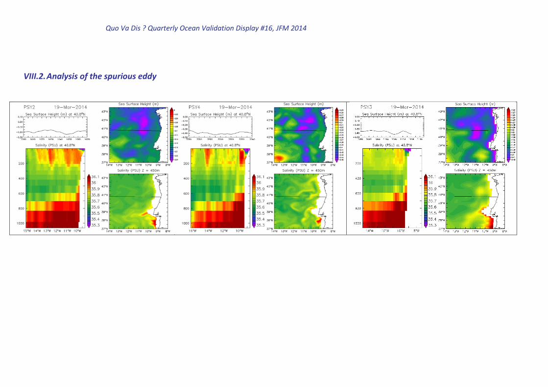
Quo Va Dis ? Quarterly Ocean Validation Display #16, JFM 2014
VIII.2. Analysis of the spurious eddy

Quo Va Dis ? Quarterly Ocean Validation Display #16, JFM 2014

Quo Va Dis ? Quarterly Ocean Validation Display #16, JFM 2014
Figure 66: description of the spurious eddy event in PSY2 (left column), PSY4 (middle column) and PSY3 (right column). Each line is for a given date in 2014. Each panel include a snapshot
of SSH (upper right corner), salinity at 450m (lower right corner), and along the black line over imposed on SSH: the SSH section (upper left corner) and salinity section (lower left corner).
In PSY2 as in PSY4, the eddy was detected from 20 March 2014. It strengthened on 26 March and propagated westward, together with strong fresh anomalies
from the surface to 400m, as can be seen in Figure 66. Nothing similar could be detected in PSY3. The spurious eddy finally faded away in PSY2 and PSY4 in
September 2014 (not shown).

Quo Va Dis ? Quarterly Ocean Validation Display #16, JFM 2014
86
VIII.3. Causes for the apparition and maintenance of the eddy
a)
b)
c)
d)
Figure 67: PSY2 innovation (a and c) and increments (b and b) of temperature (°C) near 0m (a and b) and near 100m (c and d).

Quo Va Dis ? Quarterly Ocean Validation Display #16, JFM 2014
87
a)
b)
c)
d)
Figure 68 : PSY2 innovation (a and c) and increments (b and b) of salinity (psu) near 0m (a and b) and near 100m (c and d).

Quo Va Dis ? Quarterly Ocean Validation Display #16, JFM 2014
88
a)
b)
c)
Figure 69: PSY2 SLA (m) innovation (a) and increment (b) on 26 March 2014. PSY2 SST (°C) increment (c) on the same date.
The routine validation procedure relies mainly on innovations (observation – forecast) or residuals
(analysis-forecast) at the time and location of the observations. Not many in situ observations were
present in the area, and all systems display large innovations in many regions from time to time (Figure 67,
Figure 68). Further analysis of all increments (corrections applied to the model) over the whole month of
March was needed in order to understand why this eddy appears and why it is not corrected by the data
assimilation system. This study mainly shows diagnostics issued from PSY2, but comments on the data
assimilation processes at play can also be applied to PSY4.
On the analysis of 26 March 2014, unusually strong salinity and temperature increments were diagnosed
along the coast of Portugal, on the whole water column (Figure 67, Figure 68) while SST and SLA
increments remained small (Figure 69). The temperature and salinity increments displayed very strong
spatial variability bounded by a circular shape. This is linked with the fact that the analysis is localized,
inside correlation radii of around 100 km. This suggests that a very strong innovation has been ingested by
the system inside this circular shape on the analysis of 26 March 2014. Then, the incremental analysis
update has started to apply the increment 7 days before that date, explaining that the spurious eddy
appeared around 20 March 2014.
After a careful examination of the individual profiles, an anomaly can be diagnosed within the circular area
on a specific profile for 22 March 2014.

Quo Va Dis ? Quarterly Ocean Validation Display #16, JFM 2014
89
a)
b)
c)
Figure 70: salinity observed, forecasted and analysed (a) and salinity misfit, residual and increment (b) computed by
PSY2V4R4 at a given profile on 22 March 2014 at 10.18w and 40.85 n. (c): The same observed salinity profile(psu, black
crosses) together with the PSY4 analysis counterpart (red line) the WOA09 climatology counterpart (blue crosses) and
another concurrent observed profile a little south from this position (pink squares).

Quo Va Dis ? Quarterly Ocean Validation Display #16, JFM 2014
90
A second profile displays the same type of anomaly a few days later, very close to the first one (Figure 71).
a)
b)
Figure 71: salinity observed, forecasted and analysed (a) and salinity misfit, residual and increment (b) computed by
PSY2V4R4 at a given profile on 1st
April 2014 at 9.58w and 40.84 n.
As can be seen in Figure 70 and Figure 71 the observed salinity profiles and the forecast profiles are distant
by 0.5 psu on the whole water column. These salinity profiles can be found in the current
CORIOLIS/CMEMS database with a flag equal to 3 (which means there is a doubt). In real time the flag was
1 (meaning the profile is good). This means that the delayed mode QC performed by CORIOLIS has
discarded these profiles, while the real time quality control of input observations for data assimilation,
based on GLORYS2V1 (1992-2009) innovations, failed to discard them.

Quo Va Dis ? Quarterly Ocean Validation Display #16, JFM 2014
91
a)
b)
Figure 72: Altika (a) and CRYOSAT2 (b) SLA tracks on the 3 April (a) and 6 April (b). The observed track positions (red quares)
are overimposed on the PSY2 SLA analysis on the same date (upper panels), and the along track observations (red squares
again) are plotted together with their PSY2 analysis counterpart (black triangles, lower panels).
Strong innovations are often diagnosed at in situ profiles (either erroneous profiles or large local errors)
but these large errors do not always generate such problems in the systems. In this case, several
limitations of the current system added up to generate and maintain this spurious eddy:
• The in situ profiles were not discarded by the QC because the QC is done for each level, and for one
level only this type of bias can be tolerated. As the bias is present on the whole water column it has
a strong effect on the system.
• This region experiences high mesoscale activity, especially in PSY2 and PSY4, thus the error
covariances are strong, leading to strong increments within the radius of influence
• For the same reason, this strong eddy was amplified and propagated by the model dynamics
• As can be seen in Figure 72 altimetry assimilation could have damped this spurious circulation but
did not work properly. This weakness of altimetry correction can be explained by the fact that
prescribed errors are too large, especially in regions close to the coast. Note also that the mean
dynamic topography (MDT) uncertainties are large in coastal regions.
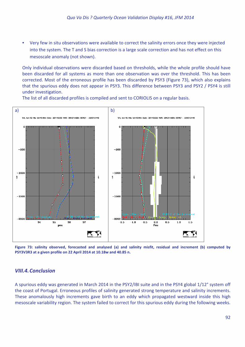
Quo Va Dis ? Quarterly Ocean Validation Display #16, JFM 2014
92
• Very few in situ observations were available to correct the salinity errors once they were injected
into the system. The T and S bias correction is a large scale correction and has not effect on this
mesoscale anomaly (not shown).
Only individual observations were discarded based on thresholds, while the whole profile should have
been discarded for all systems as more than one observation was over the threshold. This has been
corrected. Most of the erroneous profile has been discarded by PSY3 (Figure 73), which also explains
that the spurious eddy does not appear in PSY3. This difference between PSY3 and PSY2 / PSY4 is still
under investigation.
The list of all discarded profiles is compiled and sent to CORIOLIS on a regular basis.
a)
b)
Figure 73: salinity observed, forecasted and analysed (a) and salinity misfit, residual and increment (b) computed by
PSY3V3R3 at a given profile on 22 April 2014 at 10.18w and 40.85 n.
VIII.4. Conclusion
A spurious eddy was generated in March 2014 in the PSY2/IBI suite and in the PSY4 global 1/12° system off
the coast of Portugal. Erroneous profiles of salinity generated strong temperature and salinity increments.
These anomalously high increments gave birth to an eddy which propagated westward inside this high
mesoscale variability region. The system failed to correct for this spurious eddy during the following weeks.

Quo Va Dis ? Quarterly Ocean Validation Display #16, JFM 2014
93
This event has been analyzed and corrective actions were decided. Most of the conditions that have made
this event possible should disappear in the next versions of the system, to be released in 2016.
The erroneous profiles fell through the cracks. This would not have been the case if a test had been
performed on dynamic height (to be implemented in the next versions of the system). Hopefully, this new
real time QC will help detecting more erroneous profiles displaying a constant offset on the vertical, and
complement the information that is regularly sent for the delayed mode QC of CORIOLIS.
Once the eddy is generated, the system does not correct sufficiently because not many in situ observations
are available to correct the salinity on the whole water column. Several other things limit the action of the
multivariate system, among which the MDT uncertainties, limiting the action of altimetry assimilation.
Also, the prescribed observations errors are too large in the current systems. The next versions of the
system will use adaptive observation errors, and a new version of the MDT corrected with GOCE
observations. As can be seen in Figure 74 the future release of the MDT strongly reduces the anticyclonic
eddy that was present near 11°W and 41°N. This feature is thus a preferred circulation feature for the
current PSY4 and PSY2 systems, imposed via SLA assimilation and the use of an MDT still containing many
uncertainties. This case will be studied in the next version of PSY4, for which the whole 2007-2015 period is
currently replayed.
a)
b)

Quo Va Dis ? Quarterly Ocean Validation Display #16, JFM 2014
94
Figure 74: Mean Dynamic Topography (m) currently in use in the PSY systems (a) and a version corrected with GOCE
observations (b) to be used in future versions of the systems.
Quo Va Dis ? Quarterly Ocean Validation Display #16, JFM 2014
95
I Annex A
I.1. Table of figures
Figure 1: schematic of the operational forecast scenario for IBI36Q (green) and PSY2Q (blue). Solid lines are the PSY2
weekly hindcast and nowcast experiments, and the IBI36 spin up. Dotted lines are the weekly 14-day forecast,
dashed lines are daily updates of the ocean forecast forced with the latest ECMWF atmospheric analysis and
forecast. The operational scenario of PSY3, PSY4 and PSY3Q, PSY4Q is similar to PSY2’s scenario. In the case of PSY4,
only weekly hindcast, nowcast and 7-day forecast are performed. ............................................................ 6 Figure 2: schematic of the operational forecast scenario for BIOMER.. ................................................................ 7 Figure 3: Weekly statistics of SLA assimilation (left: global, right: Indian ocean zone). ...................................... 10 Figure 4 : Jason2 (up) and Cryosat2 (down) coverage during one week in February 2014 (left) and September 2013 (right).
.................................................................................................................................................................... 11 Figure 5: Seasonal JFM 2014 temperature anomalies with respect to GLORYS2V3 climatology (1993-2011). (a): SST
anomaly (°C) at the global scale from the 1/4° ocean monitoring and forecasting system PSY3V3R3. (b): heat
content anomaly (ρ0Cp∆T, with constant ρ0=1020 kg/m3 ) from the surface to 300m. ............................. 13 Figure 6: Seasonal JFM 2014 temperature anomaly (°C) with respect to GLORYS2V3 climatology (1993-2011), vertical
section 2°S-2°N mean, Pacific Ocean, PSY3V3R3. ...................................................................................... 14 Figure 7 : Arctic sea ice extent from the NSIDC, available at http://nsidc.org/arcticseaicenews ....................... 14 Figure 8 : Comparison between SLA data assimilation scores (a: average misfit in cm, b: RMS misfit in cm, c: number of
observations) for all available Mercator Ocean systems in JFM 2014. The scores are averaged for all available
satellite along track data (Saral/altiKa, Jason 2, Cryosat 2). For each region the bars refer to PSY2V4R4 (yellow),
PSY3V3R3 (red), PSY4V2R2 (blue). ............................................................................................................. 15 Figure 9: Comparison between SLA data assimilation scores (a: average misfit in cm, b: RMS misfit in cm, c: number of
observations) for all available Mercator Ocean systems in JFM 2014 in sub-regions of the Tropical Atlantic (TAT) and
North Atlantic (NAT). The scores are averaged for all available satellite along track data (Jason 1 G, Jason 2, Cryosat
2). For each region the bars refer respectively to PSY2V4R4 (yellow), PSY3V3R3 (red), and PSY4V2R2 (blue). 16 Figure 10: Comparison between SLA data assimilation scores (a: average misfit in cm, b: RMS misfit in cm, c: number of
observations) for all available Mercator Ocean systems in JFM 2014 in the Mediterranean Sea MED sub-regions:
PSY2V4R4 (yellow), PSY3V3R3 (red) and PSY4V2R2 (blue). The scores are averaged for all available satellite along
track data (Jason 1 G, Jason 2, Cryosat 2). See annex B for geographical location of regions. .................. 17 Figure 11: Comparison between SLA data assimilation scores (a: average misfit in cm, b: RMS misfit in cm, c: number of
observations) for all available global Mercator Ocean systems in JFM 2014 in sub-regions of the SAT, IND, NPA, SPA,
TPA, and ACC basins: PSY3V3R3 (red) and PSY4V2R2 (blue). The scores are averaged for all available along track
satellite data (Jason 1 G, Jason 2, Cryosat 2). The geographical location of regions is displayed in annex B.18 Figure 12: Comparison between Reynolds ¼°AVHRR-data assimilation scores (a: average misfit in °C, b: RMS misfit in °C, c:
number of observations) for all available Mercator Ocean systems in JFM 2014: PSY4V2R2 (blue), PSY3V3R3 (red),
and PSY2V4R4 (yellow). .............................................................................................................................. 19 Figure 13: Comparison between Reynolds ¼°AVHRR SST data assimilation scores (a: average misfit in °C, b: RMS misfit in
°C, c: number of observations) for all available Mercator Ocean systems in JFM 2014 in sub-regions of the Tropical
Atlantic (TAT) and of the North Atlantic (NAT): PSY4V2R2 (blue), PSY3V3R3 (red) and PSY2V4R4 (yellow). The
geographical location of regions is displayed in annex B. .......................................................................... 20 Figure 14: Comparison between Reynolds ¼° AVHRR SST data assimilation scores (a: average misfit in °C, b: RMS misfit in
°C, c: number of observations) for all available Mercator Ocean systems in JFM 2014 in the Mediterranean Sea:
PSY4V2R2 (blue), PSY3V3R3 (red) and PSY2V4R4 (yellow). The geographical location of regions is displayed in annex
B. ................................................................................................................................................................. 21 Figure 15: Comparison between Reynolds ¼° AVHRR SST data assimilation scores (a: average misfit in °C, b: RMS misfit in
°C, c: number of observations) for all available global Mercator Ocean systems in JFM 2014 in the SAT, NPA, TPA,
SPA, IND and ACC basins: PSY3V3R3 (red) and PSY4V2R2 (blue). See annex B for geographical location of regions.
.................................................................................................................................................................... 22

Quo Va Dis ? Quarterly Ocean Validation Display #16, JFM 2014
96
Figure 16: Profiles of JFM 2014 innovations of temperature (°C, left column) and salinity (psu, right column), mean (solid
line) and RMS (dashed line) for PSY3V3R3 (red), PSY2V4R4 (yellow) and PSY4V1R3 (blue) in the North Atlantic NAT
(a and b), Mediterranean Sea MED (c and d) and Arctic Ocean ARC (e an fl, the region starts of north of 67°N). Basin
masks are applied to keep only the main basin of interest (no Mediterranean in the Altantic NAT, no Black Sea in the
Mediterranean MED, etc…). ....................................................................................................................... 24 Figure 17: As Figure 16 in the Tropical Atlantic TAT (a and b), South Atlantic SAT (c and d) and Indian IND (e and f) basins.
.................................................................................................................................................................... 26 Figure 18: As Figure 16 in the North Pacific NPA (a and b), Tropical Pacific TPA (c and d) and South Pacific SPA (e and f).
.................................................................................................................................................................... 28 Figure 19: As Figure 16 in the ACC Southern Ocean basin (from 35°S). .............................................................. 29 Figure 20: As Figure 16 in the North East Atlantic (IBI) and the North Madeira XBT regions. ............................. 30 Figure 21: As Figure 16 in the Dakar region. ........................................................................................................ 31 Figure 22: As Figure 16 in the Ascension tide (a and b), the Gulf of Mexico (c and d) and the Gulf Stream 1 regions (e and f)
.................................................................................................................................................................... 32 Figure 23:number of observations of T (a) and S (b) assimilated in PSY4V2R2 in the Gulf Stream 1 region during the JFM
2014 quarter. .............................................................................................................................................. 33 Figure 24: As Figure 16 in the Algerian (a and b), the gulf of Lion (c and d), the Ionian (e and f) and the Mersa Matruh (g
and h) regions. ............................................................................................................................................ 35 Figure 25: As Figure 16 in the North West Indian (a and b), the South West Indian (c and d) and the East Indian (e and f)
regions ........................................................................................................................................................ 37 Figure 26: Average difference MODEL-OBSERVATION of temperature (a, c, and e, in °C) and salinity (b, d, and f, in psu) in
JFM 2014 between the daily average hindcast PSY4V2R2 (a and b), PSY3V3R3 (c and d) and PSY2V4R4 (e and f)
hindcast products and all available T/S observations from the Coriolis database. The Mercator hindcast products are
taken at the time and location of the observations. Averages are performed in the 0-50m layer. The size of the pixel
is proportional to the number of observations used to compute the RMS in 2°x2° boxes. ....................... 39 Figure 27: RMS temperature (°C) difference (model-observation) in JFM 2014 between all available T/S observations from
the Coriolis database and the daily average hindcast PSY3V3R3 products on the left and hindcast PSY4V2R2 on the
right column colocalised with the observations. Averages are performed in the 0-50m layer (a and b) and in the 0-
500m layer (c and d). The size of the pixel is proportional to the number of observations used to compute the RMS
in 2°x2° boxes. ............................................................................................................................................ 40 Figure 28: RMS salinity (psu) difference (model-observation) in JFM 2014 between all available T/S observations from the
Coriolis database and the daily average hindcast PSY3V3R3 products (a and c) and hindcast PSY4V2R2 (b and d),
colocalised with the observations. Averages are performed in the 0-50m layer (a and b) and in the 0-500m layer (c
and d). The size of the pixel is proportional to the number of observations used to compute the RMS in 2°x2° boxes.
.................................................................................................................................................................... 41 Figure 29 : JFM 2014 global statistics of temperature (°C, a and c) and salinity (psu, b and d) averaged in 6 consecutive
layers from 0 to 5000m. RMS difference (a and b) and mean difference (observation-model, c and d) between all
available T/S observations from the CORIOLIS database and the daily average hindcast products PSY3V3R3 (red),
PSY4V2R2 (blue) and WOA09 climatology (grey) colocalised with the observations. NB: average on model levels is
performed as an intermediate step which reduces the artefacts of inhomogeneous density of observations on the
vertical. ....................................................................................................................................................... 42 Figure 30: RMS difference (model-observation) of temperature (a and b, °C) and salinity (c and d, psu) in JFM 2014
between all available T/S observations from the Coriolis database and the daily average PSY2V4R4 hindcast
products colocalised with the observations in the 0-50m layer (a and c) and 0-500m layer (b and d) ..... 43 Figure 31: Water masses (Theta, S) diagrams in JFM 2014 in the Bay of Biscay (a to c), Gulf of Lion (d to f), Irminger Sea (g
to i) and Gulf of Cadiz (j to l), comparison between PSY3V3R3 (a, d, g, j), PSY4V2R2 (b, e, h, k) and PSY2V4R4 (c, f, I,
and l) in AMJ 2013. PSY2, PSY3 and PSY4: yellow dots; Levitus WOA09 climatology: red dots; in situ observations:
blue dots. .................................................................................................................................................... 45 Figure 32 : Water masses (T, S) diagrams in the Western Tropical Atlantic (a to c) and in the Eastern Tropical Atlantic (d to
f) in JFM 2014: for PSY3V3R3 (a, d); PSY4V2R2 (b, e); and PSY2V4R4 (c, f). PSY2, PSY3 and PSY4: yellow dots; Levitus
WOA09 climatology; red dots, in situ observations: blue dots. ................................................................. 46 Figure 33: Water masses (T, S) diagrams in South Africa (a and b), Kuroshio (c and d), and Gulf Stream region (e and f): for
PSY3V3R1 (a, c and e); PSY4V1R3 (b, d and f) in JFM 2014. PSY3 and PSY4: yellow dots; Levitus WOA09 climatology:
red dots; in situ observations: blue dots. ................................................................................................... 48

Quo Va Dis ? Quarterly Ocean Validation Display #16, JFM 2014
97
Figure 34 : RMS temperature (°C) differences between OSTIA daily analyses and PSY3V3R3 daily analyses (a); between
OSTIA and PSY4V2R2 (b), between OSTIA and PSY2V4R4 (c) in JFM 2014. The Mercator Océan analyses are
colocalised with the satellite observations analyses. ................................................................................. 49 Figure 35: Mean SST (°C) daily differences in JFM 2014 between OSTIA daily analyses and PSY3V3R3 daily analyses (a),
between OSTIA and PSY4V2R2 (b) and between OSTIA and PSY2V4R4 daily analyses (c)......................... 49 Figure 36: Near surface (15m) zonal current (m/s) comparison between the Mercator systems analyses and observed
velocities from drifters. In the left column: velocities collocated with drifter positions in JFM 2014 for PSY3V3R3 (a),
PSY4V2R2 (c) and PSY2V4R4 (e). In the right column, zonal current from drifters in JFM 2014 (b) at global scale,
AOML drifter climatology for JFM with new drogue correction from Lumpkin & al, in preparation (d) and observed
zonal current in JFM 2014 (f) over PSY2’s domain. .................................................................................... 51 Figure 37 : In JFM 2014, comparison of the mean relative velocity error between in situ AOML drifters and model data (a,
c and e) and mean zonal velocity bias between in situ AOML drifters with Mercator Océan correction (see text) and
model data (b, d and f). a and b: PSY3V3R3, c and d: PSY4V2R3, e and f: PSY2V4R2. NB: zoom at 500% in order to
see the arrows. ........................................................................................................................................... 52 Figure 38: In JFM 2014, comparison of the mean distance error in 1°x1° boxes after a 1-day drift (a and b), after a 3-days
drift (c and d), and after a 5-days drift (e and f).between AOML drifters’ trajectories and PSY3V3R3 trajectories (a, c,
and e) and between AOML drifters’ trajectories and PSY4V2R2 (b,d, and f). ............................................ 53 Figure 39:Cumulative Distribution Functions of the distance error (km, on the left) and the direction error (degrees, on
the right panel) after 1 day (blue), 3 days (green) and 5 days (red), between PSY4V1R3 forecast trajectories and
actual drifters trajectories. ......................................................................................................................... 54 Figure 40: Arctic (a to c) and Antarctic (d to f) JFM 2014 Sea ice cover fraction in PSY3V3R3 (a and d), in CERSAT
observations (b and e) and difference PSY3 – CERSAT (c and f). ................................................................ 55 Figure 41: Arctic (a to c) and Antarctic (d to f) JFM 2014 Sea ice cover fraction in PSY4V2R2 (a and d), in CERSAT
observations (b and e) and difference PSY4 – CERSAT (c and f). ................................................................ 56 Figure 42: JFM 2014 Arctic sea ice extent in PSY4V2R2 with overimposed climatological AMJ 1992-2010 sea ice fraction
(magenta line, > 15% ice concentration) (a) and NSIDC map of the sea ice extent in the Arctic for March 2014 in
comparison with a 1979-2000 median extend (b). .................................................................................... 57 Figure 43 : Mean bias (model-observation) (a), RMS error (b), correlation (c) between IBI36V2 and analysed L3 SST from
Météo-France CMS for the JFM 2014 quarter. Same diagnostics for PSY2V4R4 (d,e,f) and PSY4V2R2 (g,h,i). Number
of Météo-France CMS observations for the JFM 2014 quarter (j). ............................................................ 58 Figure 44 : Over the whole IBI36V2 domain (a and b) and over the Bay of Biscay (c and d): mean “IBI36V2 - observation”
temperature (°C) bias (red) and RMS error (blue) in JFM 2014 (a and c), and mean profile from IBI36V2 (black),
PSY2V4R4 (green) and from the observations (red) in JFM 2014 (b and d). In the lower right corner of each plot:
position of the individual profiles. .............................................................................................................. 59 Figure 45: Over the whole IBI36V2 domain (a and b) and over the Bay of Biscay (c and d): mean “IBI36V2 - observation”
salinity (psu) bias (red) and RMS error (blue) in JFM 2014 (a and c), and mean profile from IBI36V2 (black),
PSY2V4R4 (green) and from the observations (red) in JFM 2014 (b and d). In the lower right corner of each plot:
position of the individual profiles. .............................................................................................................. 60 Figure 46 : Mixed Layer Depth distribution in JFM 2014 in IBI36V2 (a and b) and PSY2V4R4 (c and d), calculated from
profiles with the temperature criteria (difference of 0.2°C with the surface); the models are in grey, the
observations in red. a and c: classification for the whole IBI domain, b and d: classification for the Bay of Biscay.
.................................................................................................................................................................... 62 Figure 47 : For IBI36V2: RMS error (a, in cm) and correlation (b) for the non-tidal Sea Surface Elevation at tide gauges in
JFM 2014, for different regions and frequencies. ...................................................................................... 63 Figure 48 : For IBI36V2: Bias (observation-model) (a, d and g), RMS error (°C) (b, e and h) and correlation (c, f and i) of the
Sea Surface Temperature between IBI36 and moorings measurements in January (a to c), February (d to f) and
March 2014 (g to i). .................................................................................................................................... 64 Figure 49: Surface temperature (°C) time series at a selection of moorings which locations are shown on the upper left
panel (no observation for Gulf of Lion). ..................................................................................................... 65 Figure 50 : Chlorophyll-a concentration (mg/m
3) in January (a and b), February (c and d) and March 2014 (e and f) for the
Mercator system BIOMER (a, c, and e) and Chlorophyll-a concentration from Globcolour (b, d and f). ... 66 Figure 51 : Probability Density Function (PDF) of Chl-a bias in log scale (log10(obs)-log10(model)) in the North Atlantic (30-
70N; 80W:20E) for January (a), February (b) and March (c) 2014. ............................................................ 67 Figure 52 : RMS difference between BIOMER and Globcolour Chl-a concentrations (mg/m
3) in JFM 2014. ...... 67

Quo Va Dis ? Quarterly Ocean Validation Display #16, JFM 2014
98
Figure 53: Schematic of the change in atmospheric forcings applied along the 14-day ocean forecast. ............ 68 Figure 54: Accuracy intercomparison in the North Atlantic region for PSY2V4R4 in temperature (a and c) and salinity (b
and dl) between hindcast (green), nowcast (yellow), 3-day (orange) and 6-day (red) forecast and WO09 climatology
(grey). Accuracy is measured by a mean difference (a and b) and by a rms difference (c and d) of temperature and
salinity with respect to all available observations from the CORIOLIS database averaged in 6 consecutive layers from
0 to 5000m. All statistics are performed for the JFM 2014 period. NB: average on model levels is performed as an
intermediate step which reduces the artefacts of inhomogeneous density of observations on the vertical. 69 Figure 55: Accuracy intercomparison in the Mediterranean Sea region for PSY2V4R4 in temperature (°C, a and c) and
salinity (psu, b and d) between hindcast, nowcast, 3-day and 6-day forecast and WO09 climatology. Accuracy is
measured by a rms difference (c and d) and by a mean difference (a and b) with respect to all available observations
from the CORIOLIS database averaged in 6 consecutive layers from 0 to 5000m. All statistics are performed for the
JFM 2014 period. NB: average on model levels is performed as an intermediate step which reduces the artefacts of
inhomogeneous density of observations on the vertical. .......................................................................... 70 Figure 56: (Obs-model) mean differences in temperature (°C, a, c, and e) and salinity (psu, b, d, and f) for PSY3V3R3 (red),
PSY2V4R4 (yellow) and PSY4V2R2 (blue) systems in the Tropical Atlantic (a and b), the Tropical Pacific (c and d) and
the Indian Ocean (e and f) in JFM 2014. ..................................................................................................... 72 Figure 57: same as Figure 54 but for RMS statistics and for temperature (°C), PSY3V3R3 and PSY4V2R2 systems and the
Tropical Atlantic (a and b), the Tropical Pacific (c and d) and the Indian Ocean (e and f). The global statistics are also
shown for temperature (°C, g and h) and salinity (psu, I and j). The right column compares the analysis of the global
¼° PSY3V3R3 (red) with the analysis of the global 1/12° PSY4V2R2 (blue). ............................................... 74 Figure 58: Temperature (left) and salinity (right) skill scores in 4°x4° bins and in the 0-500m layer in JFM 2014 in
PSY3V3R3 (a and b) , PSY4V2R2 (c and d) and PSY2V4R4 (e and f). The skill illustrates the ability of the 3-days
forecast to be closer to in situ observations than the persistence of the analysis, see Equation 1. Yellow to red
values indicate that the forecast is more accurate than the persistence. ................................................. 75 Figure 59 : As Figure 58 but the reference is the WOA 2009 climatology. Temperature (a and c) and salinity (b and d) skill
scores are displayed for JFM 2014, for PSY3V3R3 (a and b) and for PSY2V4R4 (c and d). The skill illustrates the ability
of the 3-days forecast to be closer to in situ observations than the climatology, see Equation 1. Yellow to red values
indicate that the forecast is more accurate than the climatology. ............................................................ 76 Figure 60: daily SST (°C) spatial mean for a one year period ending in AMJ 2013 for PSY2V4R4 (a), PSY3V3R3 (b), and
PSY4V2R1 until 31/10/2012 then PSY4V2R2 (c). Mercator Ocean systems are in black and Reynolds AVHRR ¼°
analysis in red. ............................................................................................................................................ 77 Figure 61: surface eddy kinetic energy EKE (m²/s²) for PSY3V3R3 (a) and PSY4V2R2 (b) for JFM 2014. ............. 78 Figure 62: Comparisons between JFM 2014 mean temperature (°C, a to c) and salinity (psu, d to f) profiles in Mercator
systems (black): PSY2V4R4 (a and d), PSY3V3R3 (b and e) and PSY4V2R2 (c and f), and in the Levitus WOA05 (green)
and ARIVO (red) monthly climatologies. .................................................................................................... 79 Figure 63: Sea ice area (a, 10
6 km2) and extent (b, 10
6 km2) in PSY3V3R3 (blue line), PSY4V1R3 until October then
PSY4V2R2 (black line) and SSM/I observations (red line) for a one year period ending in JFM 2014, in the Arctic
(upper panel) and Antarctic (lower panel). ................................................................................................ 80 Figure 64: difference between the IBI36 SLA and merged SLA observations from AVISO (m) , (a) for a date in March, (b) in
April and (c) in May. ................................................................................................................................... 81 Figure 65: SST analyses (°C) from PSY2 and PSY4 colocated with L3S high frequency SST observations from Météo-
France/CMS. (a) between March 26 and April 2, (b) between April 2 and April 8. .................................... 82 Figure 66: description of the spurious eddy event in PSY2 (left column), PSY4 (middle column) and PSY3 (right column).
Each line is for a given date in 2014. Each panel include a snapshot of SSH (upper right corner), salinity at 450m
(lower right corner), and along the black line over imposed on SSH: the SSH section (upper left corner) and salinity
section (lower left corner). ......................................................................................................................... 85 Figure 67: PSY2 innovation (a and c) and increments (b and b) of temperature (°C) near 0m (a and b) and near 100m (c
and d). ........................................................................................................................................................ 86 Figure 68 : PSY2 innovation (a and c) and increments (b and b) of salinity (psu) near 0m (a and b) and near 100m (c and d).
.................................................................................................................................................................... 87 Figure 69: PSY2 SLA (m) innovation (a) and increment (b) on 26 March 2014. PSY2 SST (°C) increment (c) on the same
date. ........................................................................................................................................................... 88 Figure 70: salinity observed, forecasted and analysed (a) and salinity misfit, residual and increment (b) computed by
PSY2V4R4 at a given profile on 22 March 2014 at 10.18w and 40.85 n. (c): The same observed salinity profile(psu,
Quo Va Dis ? Quarterly Ocean Validation Display #16, JFM 2014
99
black crosses) together with the PSY4 analysis counterpart (red line) the WOA09 climatology counterpart (blue
crosses) and another concurrent observed profile a little south from this position (pink squares). ......... 89 Figure 71: salinity observed, forecasted and analysed (a) and salinity misfit, residual and increment (b) computed by
PSY2V4R4 at a given profile on 1st
April 2014 at 9.58w and 40.84 n. ........................................................ 90 Figure 72: Altika (a) and CRYOSAT2 (b) SLA tracks on the 3 April (a) and 6 April (b). The observed track positions (red
quares) are overimposed on the PSY2 SLA analysis on the same date (upper panels), and the along track
observations (red squares again) are plotted together with their PSY2 analysis counterpart (black triangles, lower
panels). ....................................................................................................................................................... 91 Figure 73: salinity observed, forecasted and analysed (a) and salinity misfit, residual and increment (b) computed by
PSY3V3R3 at a given profile on 22 April 2014 at 10.18w and 40.85 n. ...................................................... 92 Figure 74: Mean Dynamic Topography (m) currently in use in the PSY systems (a) and a version corrected with GOCE
observations (b) to be used in future versions of the systems. ................................................................. 94 Figure 75 : illustration of QC: Quality test example chosen for windage (eg. 1%) we reject or correct a drift that differs
little from the windage (less than 70% of the drift angle <40 °) .............................................................. 103 Figure 76: Example of the surface currents Lagrangian quality control algorithm on a global map (bottom panel) and
zooms (upper panels). .............................................................................................................................. 104 Figure 77: Illustration of the surface currents Lagrangian quality control algorithm. ....................................... 105

Quo Va Dis ? Quarterly Ocean Validation Display #16, JFM 2014
100
II Annex B
II.1. Maps of regions for data assimilation statistics
II.1.1. Tropical and North Atlantic
1 Irminger Sea 12 Puerto Rico XBT
2 Iceland Basin 13 Dakar
3 Newfoundland-Iceland 14 Cape Verde XBT
4 Yoyo Pomme 15 Rio-La Coruna Woce
5 Gulf Stream2 16 Belem XBT
6 Gulf Stream1 XBT 17 Cayenne tide
7 North Medeira XBT 18 Sao Tome tide
8 Charleston tide 19 XBT - central SEC
9 Bermuda tide 20 Pirata
10 Gulf of Mexico 21 Rio-La Coruna
11 Florida Straits XBT 22 Ascension tide

Quo Va Dis ? Quarterly Ocean Validation Display #16, JFM 2014
101
I.1.1. Mediterranean Sea
1 Alboran 8 Ionian
2 Algerian 9 Egee
3 Lion 10 Ierepetra
4 Thyrrhenian 11 Rhodes
5 Adriatic 12 MersaMatruh
6 Otranto 13 Asia Minor
7 Sicily

Quo Va Dis ? Quarterly Ocean Validation Display #16, JFM 2014
102
I.1.2. Global ocean
1 Antarctic Circumpolar Current 13 Nino3
2 South Atlantic 14 Nino4
3 Falkland current 15 Nino6
4 South Atl. gyre 16 Nino5
5 Angola 17 South tropical Pacific
6 Benguela current 18 South Pacific Gyre
7 Aghulas region 19 Peru coast
8 Pacific Region 20 Chile coast
9 North Pacific gyre 21 Eastern Australia
10 California current 22 Indian Ocean
11 North Tropical Pacific 23 Tropical indian ocean
12 Nino1+2 24 South indian ocean

Quo Va Dis ? Quarterly Ocean Validation Display #16, JFM 2014
103
II Annex C
II.1.Quality control algorithm for the Mercator Océan drifter data correction (Eric Greiner)
Before estimating the bias, it is essential to conduct a quality control. We must consider an individual
monitoring of buoys, and a comparison with the geostrophy and windage. In real time, this is not possible,
and I propose below a simple test developed by position (date by date) which involves only the mean wind
(2 days) and the buoy drift. Basically, we found drifters where drift is close to argue between 0.2 and 3% of
the wind (almost the same direction with a drag corresponding to a loss of drogue). For these buoys, if the
contamination is real, then the error due to the wind is important with respect to current real at 15m
depth. We test different values of windage (wind effect for a fraction of a given wind between 0.2% and
3%). If a questionable observation is found for a given windage, we estimate a correction. We apply at the
end an average correction QC (windage among all acceptable). We although increase the error of
observation. Note that in delayed time, we could correct all the data from the buoy, at least in a 10-day
window. Note however that a buoy that has lost its drogue can give a good measure if the wind is low
• No anomaly : slippage correction of 0.07% of the 10m wind speed
• Windage > 0.2% or < 3% correction of 1% of windage
Figure 75 : illustration of QC: Quality test example chosen for windage (eg. 1%) we reject or correct a drift that differs little
from the windage (less than 70% of the drift angle <40 °)
Note that a correction of more than 3% is not normally possible (construction of the buoy). This may
correspond to breaking waves and swell. Between 2% and 3%, there is ambiguity between Stokes and
windage. In other words, it is likely that beyond 2%, we eliminate all or part of the effect of waves and
swell. If waves and swell are not aligned with the mean wind (swell remote for example), then the
correction will be approximate. Ideally, you should use the Stokes drift from a wave model like
Wavewatch3.
When calculating the equivalent models with AOML positions, which were filtered to remove 36h gravity
waves and reduce positioning errors, we must :
• add 0.07% wind averaged over 48h 10m : slippage correction
• windage correction and modify the error

Quo Va Dis ? Quarterly Ocean Validation Display #16, JFM 2014
104
II.2. Algorithm of the Lagrangian verification of the Mercator Océan surface currents forecast.
Algorithm of the Lagrangian verification of the Mercator Océan surface currents forecast. The Mercator
Océan surface currents quality control now combines two methods based on Eulerian and Lagrangian
approaches using the AOML drifters network.
The Lagrangian approach is slightly different from the Eulerian approach. In the Eulerian approach, the
consecutive positions of a drifter are considered as independent buoys recording velocity observations.
Then, these observations are compared to the modeled velocity.
We aim here at studying the trajectory of the buoy along with the trajectory of a modeled buoy which
would drift from the same starting point. The computation of the trajectory of the modeled drifter is made
possible by ARIANE (see ref 1 above)
The algorithm aims at producing the maps on Figure 76. It shows the mean 1-to-5-days distance error –that
is the distance between the modeled trajectory and the observed trajectory- in 1°x1° boxes. The mean D-
days distance error is computed by averaging the D-days distance errors computed for all the drifters that
crossed the box.
The individual points of a trajectory are not independent, merely because the location of a drifter is to a
large extent determined by its former location.
Figure 76: Example of the surface currents Lagrangian quality control algorithm on a global map (bottom panel) and zooms
(upper panels).
Let us consider the example above (Figure 77). The thin grey line represents the trajectory of the drifter on
a daily frequency. The thick ones represent the system drifting, starting from an observed point. Their

Quo Va Dis ? Quarterly Ocean Validation Display #16, JFM 2014
105
colors show the distance to the corresponding point in the observed trajectory after D-days. Considering
only this drifter, if we compute the D-days distance error starting from the t=0 observed point (01/02/2013
in the example), we may compute it again only from the observed point t=D days. This way we may
reasonably assume the two distance errors are uncorrelated and use most of the data (see ref 2 above).
Figure 77: Illustration of the surface currents Lagrangian quality control algorithm.
References:
1- Ariane : utility developed at LPO (http://wwz.ifremer.fr/lpo_eng/Produits/Logiciels/ARIANE)
2- Scott, R. B., N. Ferry, M. Drevillon, C. N. Barron, N. C. Jourdain, J.-M. Lellouche, E. J. Metzger, M.-H.
Rio, and O. M. Smedstad, Estimates of surface drifter trajectories in the equatorial Atlantic: A multi-
model ensemble approach, Ocean Dynamics, 62, 1091-1109, 2012, doi:10.1007/s10236-012-0548-
2.


![[Youdz.ru] cфера духовной жизни](https://img.pdfslide.tips/doc/110x75/545ad499af79594f558b5e25/youdzru-c-.jpg)


![[Youdz.ru] причастный оборот](https://img.pdfslide.tips/doc/110x75/5452263daf7959dd1f8b47e8/youdzru--5584b59c08bf7.jpg)