Continuous Time Series Alignment in HumanActions Recognition.

Goncharov Alexey Vladimirovich

Moscow institue of Physics and TechnologyDepartment of intellectual systems, DCAM.

Scientific supervisor: V. V. Strijov.

Conference AINL-2016

A.V. Goncharov Continuous warping path 1 / 26

Example of scientific tasks

Time series of acceleration from phone accelerometer for differenttypes of human activity

ad

A.V. Goncharov Continuous warping path 2 / 26

References

1 Petitjean F., Chen Y., Keogh E., ICDE, 2014. — DBAmethod for centrois calculating.

2 Goncharov A.V., Strijov V.V. Systems and applications ofinformatics, 2015. — reasons for using the DTW distance inthe classification task.

3 Kwapisz J. R. 2010. — Data using for human activityrecognitionhttp://sourceforge.net/p/mlalgorithms/TSLearning/data/preprocessedlarge.csv

A.V. Goncharov Continuous warping path 3 / 26

Main points

Suggest an efficient way for large multiscale time series analyzing.

Suggestions

Continuous versions of time series.

Similar to Dynamic time warping properties.

Difficulties

What the continuous time series are?

What the distance function between continuous objects is?

Warping path search can’t be solved like in the discrete case.

Benefits

Less memory space for keeping data.

Ability of working with multiscale time series.

Theoretical computing of DTW cost.

A.V. Goncharov Continuous warping path 4 / 26

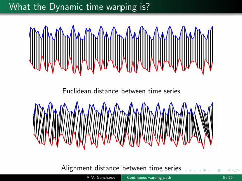
What the Dynamic time warping is?

Euclidean distance between time series

Alignment distance between time seriesA.V. Goncharov Continuous warping path 5 / 26

What the alignment path is?

Dissimilarity matrix for time series elementsΩn×n : Ω(i , j) = |s(i)− c(j)|.Path π with length K between s and c:π = πk = (ik , jk), k = 1, . . . ,K , i , j ∈ 1, ..., n

A.V. Goncharov Continuous warping path 6 / 26

Time series definition

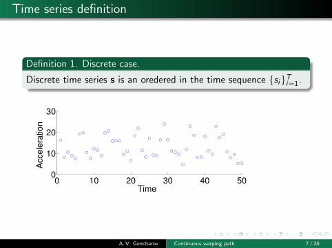
Definition 1. Discrete case.

Discrete time series s is an oredered in the time sequence siTi=1.

0 10 20 30 40 500

10

20

30

Time

Accele

ration

A.V. Goncharov Continuous warping path 7 / 26

Time series definition

Definition 1. Continuous case.

Continuous time series on time plot T = [0;T ] is a continuousfunction sc(t) : T → R.

0 10 20 30 40 500

10

20

30

Time

Accele

ration

A.V. Goncharov Continuous warping path 8 / 26

Path definition

Definition 2. Discrete case.

path π between two discrete time series s1 and s2 is anordered set of index pairs:

π = πr = (ir , jr ), r = 1, . . . ,R, i , j ∈ 1, ..., n,

and it satisfies the discrete continuity, monotony and the boundaryconditions:

πr = (p1, p2), πr−1 = (q1, q2), r = 2, ...,R, ⇒

p1 − q1 ≤ 1, p2 − q2 ≤ 1,

πr = (p1, p2), πr−1 = (q1, q2), r = 2, ...,R, ⇒

p1 − q1 ≥ 1, p2 − q2 ≥ 1,

π1 = (1, 1), πR = (n, n).

A.V. Goncharov Continuous warping path 9 / 26

Path definition

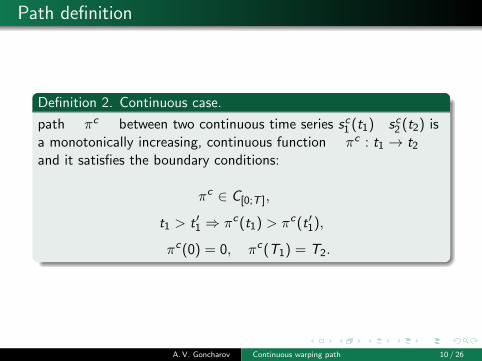
Definition 2. Continuous case.

path πc between two continuous time series sc1 (t1) sc2 (t2) isa monotonically increasing, continuous function πc : t1 → t2and it satisfies the boundary conditions:

πc ∈ C[0;T ],

t1 > t ′1 ⇒ πc(t1) > πc(t ′1),

πc(0) = 0, πc(T1) = T2.

A.V. Goncharov Continuous warping path 10 / 26

Path definition

0 20 40 600

5

10

15

20

25

30

35

40

45

Time 1

Tim

e 2

0 20 40 600

5

10

15

20

25

30

35

40

45

Time 1

Tim

e 2

Alignment paths in two cases: discrete and continuous

A.V. Goncharov Continuous warping path 11 / 26

Path cost definition

Definition 3. Discrete case.

the cost Cost(s1, s2,π) of path π with length R betweentwo discrete time series s1 and s2 is:

Cost(s1, s2,π) =1

R

∑(i ,j)∈π

|s1(i)− s2(j)|.

Definition 3. Continuous case.

the cost Cost(sc1 (t1), sc2 (t2), πc) of path πc between twocontinuous time series sc1 (t1) and sc2 (t2) is:

Cost(sc1 (t1), sc2 (t2), πc) =1

L

∫t1

|sc1 (t1)− sc2 (πc(t1))|dt1,

where L is length of the curve that is given by the graph of thefunction πc(t), t ∈ [0,T ].

A.V. Goncharov Continuous warping path 12 / 26

Warping path definition

Definition 4. Discrete case.

warping path π between two discrete time series s1 ands2 is a path that has the smallest cost among all possible paths:

π = argminπ

Cost(s1, s2,π).

Definition 4. Continuous case.

warping path πc between two continuous time seriessc1 (t1) and sc2 (t2) is a function πc that has the smallestvalue of cost from the 3rd definition:

πc = argminπc

Cost(sc1 (t1), sc2 (t2), πc).

A.V. Goncharov Continuous warping path 13 / 26

The cost of warping path

Definition 5. Discrete case.

the cost of warping path or DTW distance between two discretetime series is:

DTW(s1, s2) = Cost(s1, s2, π).

Definition 5. Continuous case.

the cost of warping path or DTW distance between two continuoustime series is:

DTW(sc1 (t1), sc2 (t2)) = Cost(sc1 (t1), sc2 (t2), πc).

A.V. Goncharov Continuous warping path 14 / 26

Dissimilarity matrix Omega

Matrix Omega for step size 0.5

Time axis 1 for sin(x)

Tim

e a

xis

2 for

sin

(x+

3)

5 10 15

2

4

6

8

10

12

14

16

18

A.V. Goncharov Continuous warping path 15 / 26

Dissimilarity matrix Omega

Matrix Omega for step size 0.25

Time axis 1 for sin(x)

Tim

e a

xis

2 for

sin

(x+

3)

5 10 15 20 25 30 35

5

10

15

20

25

30

35

A.V. Goncharov Continuous warping path 16 / 26

Dissimilarity matrix Omega

Matrix Omega for step size 0.125

Time axis 1 for sin(x)

Tim

e a

xis

2 for

sin

(x+

3)

10 20 30 40 50 60 70

10

20

30

40

50

60

70

A.V. Goncharov Continuous warping path 17 / 26

Dissimilarity matrix Omega

Matrix Omega for step size 0.015625

Time axis 1 for sin(x)

Tim

e a

xis

2 for

sin

(x+

3)

100 200 300 400 500

100

200

300

400

500

A.V. Goncharov Continuous warping path 18 / 26

The alignment path properties

Lemma 1.

s1(t) and s2(t) are two time series with Lipschitz constant L,πc : t1 → t2 is the warping path between them. Its cost does notvary greatly while there are small changes in this path:

‖ πc − πc ‖C≤ ε ⇒ |Cost(s1, s2, πc)− Cost(s1, s2, π

c)| ≤ εTL,

where T determines the time boundary for time series, ε > 0.

Lemma 2.

s1(t) and s2(t) are two time series with Lipschitz constant L,πc : t1 → t2 is the warping path between them. Its cost does notvary greatly while there are small changes in one of time series:

‖ s2 − s2 ‖C≤ ε ⇒ |Cost(s1, s2, πc)− Cost(s1, s2, π

c)| ≤ εTL,

where T determines the time boundary for time series, ε > 0.

A.V. Goncharov Continuous warping path 19 / 26

The alignment path properties

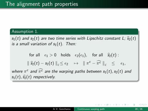
Assumption 1.

s1(t) and s2(t) are two time series with Lipschitz constant L; s2(t)is a small variation of s1(t). Then:

for all ε1 > 0 holds ε2(ε1), for all s2(t) :

‖ s2(t)− s2(t) ‖C≤ ε2 7→ ‖ πc − πc ‖

C≤ ε1,

where πc and πc are the warping paths between s1(t), s2(t) ands1(t), s2(t) respectively.

A.V. Goncharov Continuous warping path 20 / 26

Algorithm of building the warping path

The warping path search

The warping path is a solution of the optimization task fromdefinition:

πc = argminπc

Cost(sc1 (t1), sc2 (t2), πc).

Suggest to search the approximation of this solution amongthe parametric functions.

Formulate the problem in the following form:

θ = argminθ

Cost(s1, s2, θ) = argminθ

∫t1

|s1(t1)−s2(F (θ)(t1))|dt1

where F (θ) is a mapping from the parameters to theparametric functions.

A.V. Goncharov Continuous warping path 21 / 26

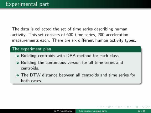
Experimental part

The data is collected the set of time series describing humanactivity. This set consists of 600 time series, 200 accelerationmeasurements each. There are six different human activity types.

The experiment plan

Building centroids with DBA method for each class.

Building the continuous version for all time series andcentroids.

The DTW distance between all centroids and time series forboth cases.

A.V. Goncharov Continuous warping path 22 / 26

Continuous version of time series

Cubic splines interpolation. One can apply any interpolation orapproximation type for getting the continuous object if moreaccurate method exists.

Figure: The example of the cubic spline interpolationA.V. Goncharov Continuous warping path 23 / 26

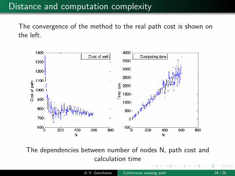
Distance and computation complexity

The convergence of the method to the real path cost is shown onthe left.

The dependencies between number of nodes N, path cost andcalculation time

A.V. Goncharov Continuous warping path 24 / 26

Averaged distance matrix

Table: The mean intraclass values.

Walk Run Up Down Sit Lie

Run 693 803 811 733 1165 1143Walk 676 498 696 610 946 927Up 714 739 696 701 1038 1021Down 591 601 653 464 836 804Sit 516 465 434 400 6 42Lie 508 441 454 366 105 79

The results for both algorithms, DTW and DTW in the continiousspace, gave following results: 85% and 83% relatively. Theseresults don’t vary greatly.

A.V. Goncharov Continuous warping path 25 / 26

Conclusion

The continuous space usage solves the problem of resamplingthe data.

Continuous DTW function has the same properties as thediscrete one.

Future plans:

Use better approximation methods.

Explore the dependence between approximation method anddistance quality.

Use more effective optimization methods for searching thebest path approximation.

Adapt DTW bounds for continuous space.

A.V. Goncharov Continuous warping path 26 / 26