Embed Size (px)
Citation preview
Machine Learning Applications forRobot Navigation and Control
E. Burnaev
Skoltech
E. Burnaev (Skoltech) ML&Robotics 1 / 33
Outline
1 Predictive Modelling in Industrial EngineeringPredictive ModellingCustomer ExpectationsSurrogate ModelsDimension Reduction
2 Robot navigation
3 ML problem statement
4 Robot control
5 Conclusions
E. Burnaev (Skoltech) ML&Robotics 2 / 33
Predictive Modelling
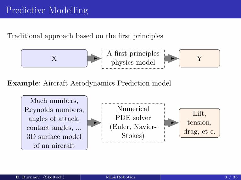
Traditional approach based on the first principles
A first principlesphysics modelX Y
Example: Aircraft Aerodynamics Prediction model
NumericalPDE solver
(Euler, Navier-Stokes)
Mach numbers,Reynolds numbers,angles of attack,contact angles, ...3D surface modelof an aircraft
Lift,tension,
drag, et c.
E. Burnaev (Skoltech) ML&Robotics 3 / 33
PM: Customer Expectations
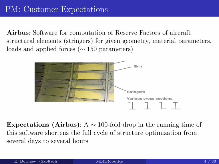
Airbus: Software for computation of Reserve Factors of aircraftstructural elements (stringers) for given geometry, material parameters,loads and applied forces (∼ 150 parameters)
Expectations (Airbus): A ∼ 100-fold drop in the running time ofthis software shortens the full cycle of structure optimization fromseveral days to several hours
E. Burnaev (Skoltech) ML&Robotics 4 / 33
SM in Engineering
PM is used in:“What-If” and Sensitivity Analysis, Design Space Exploration;Design Optimization with respect to specified efficiency criteria
Prohibitive volumes and/or run-time costs:from thousands to millions of computational experiments;running time of an experiment ranges form seconds to days;
Surrogate models: fast approximations, which substitute the originalmodels without a significant loss in accuracy
E. Burnaev (Skoltech) ML&Robotics 5 / 33
Constructing Surrogate Models
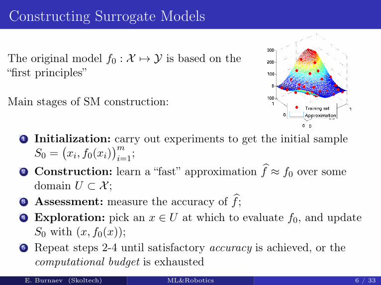
The original model f0 : X 7→ Y is based on the“first principles”
Main stages of SM construction:
1 Initialization: carry out experiments to get the initial sampleS0 =
(xi, f0(xi)
)mi=1
;2 Construction: learn a “fast” approximation f ≈ f0 over some
domain U ⊂ X ;3 Assessment: measure the accuracy of f ;4 Exploration: pick an x ∈ U at which to evaluate f0, and updateS0 with (x, f0(x));
5 Repeat steps 2-4 until satisfactory accuracy is achieved, or thecomputational budget is exhausted
E. Burnaev (Skoltech) ML&Robotics 6 / 33
Quick Aerodynamic Design of Passenger Aircraft Layout
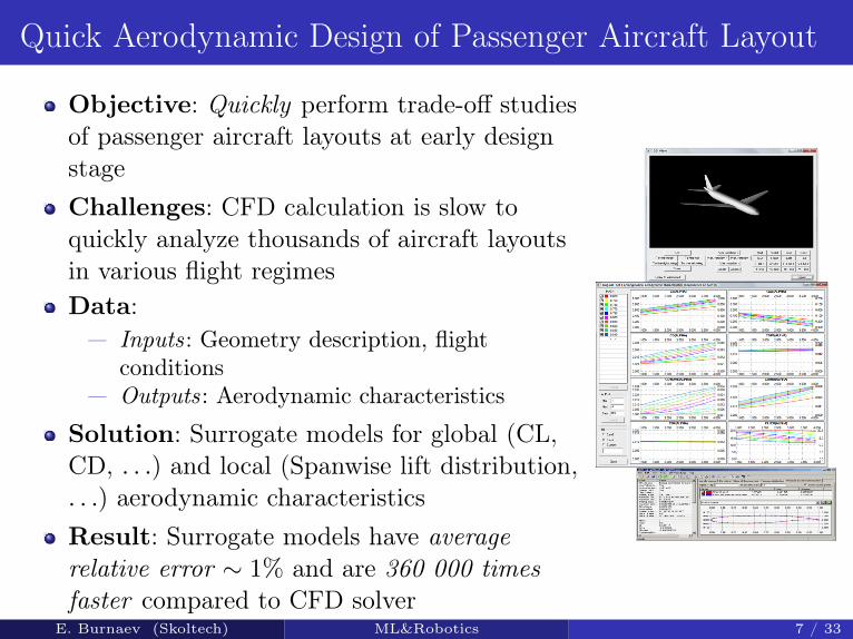
Objective: Quickly perform trade-off studiesof passenger aircraft layouts at early designstageChallenges: CFD calculation is slow toquickly analyze thousands of aircraft layoutsin various flight regimesData:— Inputs: Geometry description, flight
conditions— Outputs: Aerodynamic characteristics
Solution: Surrogate models for global (CL,CD, . . .) and local (Spanwise lift distribution,. . .) aerodynamic characteristicsResult: Surrogate models have averagerelative error ∼ 1% and are 360 000 timesfaster compared to CFD solver
E. Burnaev (Skoltech) ML&Robotics 7 / 33
Geometry Description
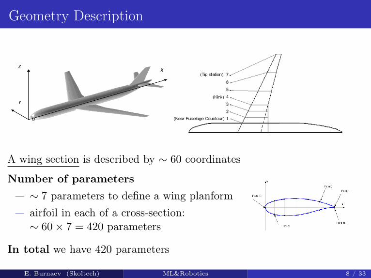
A wing section is described by ∼ 60 coordinates
Number of parameters— ∼ 7 parameters to define a wing planform— airfoil in each of a cross-section:∼ 60× 7 = 420 parameters
In total we have 420 parameters
E. Burnaev (Skoltech) ML&Robotics 8 / 33
Dimension Reduction
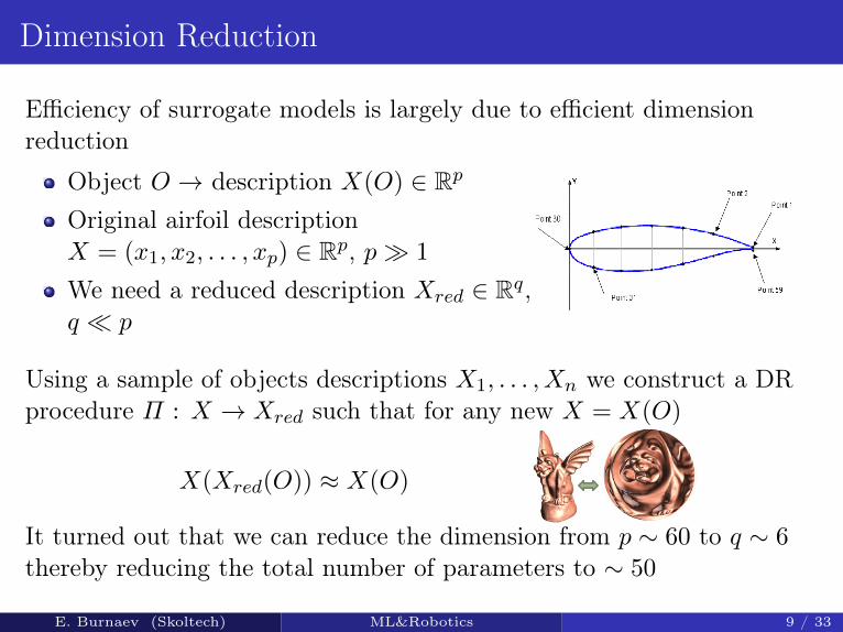
Efficiency of surrogate models is largely due to efficient dimensionreduction
Object O → description X(O) ∈ Rp
Original airfoil descriptionX = (x1, x2, . . . , xp) ∈ Rp, p� 1
We need a reduced description Xred ∈ Rq,q � p
Using a sample of objects descriptions X1, . . . , Xn we construct a DRprocedure Π : X → Xred such that for any new X = X(O)
X(Xred(O)) ≈ X(O)
It turned out that we can reduce the dimension from p ∼ 60 to q ∼ 6thereby reducing the total number of parameters to ∼ 50
E. Burnaev (Skoltech) ML&Robotics 9 / 33
DR and SM: Challenges
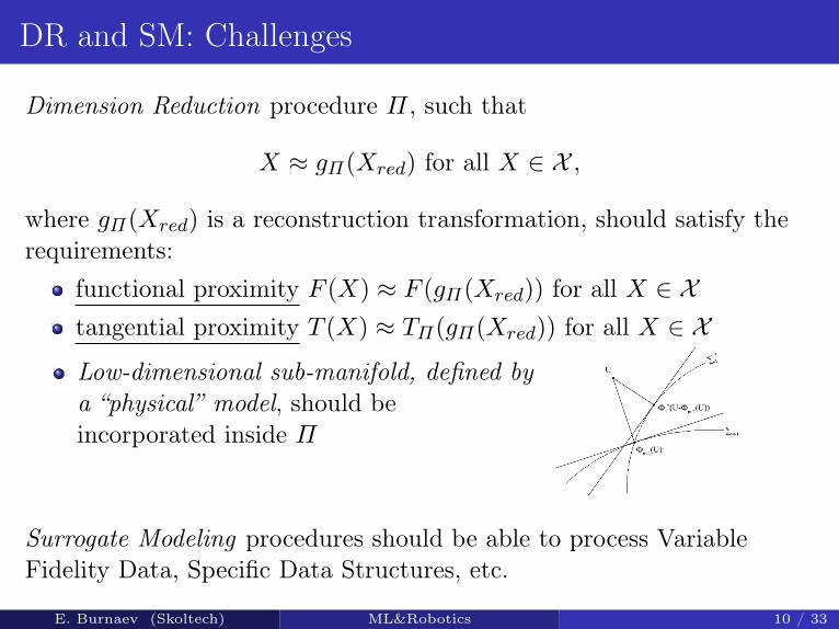
Dimension Reduction procedure Π, such that
X ≈ gΠ(Xred) for all X ∈ X ,
where gΠ(Xred) is a reconstruction transformation, should satisfy therequirements:
functional proximity F (X) ≈ F (gΠ(Xred)) for all X ∈ Xtangential proximity T (X) ≈ TΠ(gΠ(Xred)) for all X ∈ X
Low-dimensional sub-manifold, defined bya “physical” model, should beincorporated inside Π
Surrogate Modeling procedures should be able to process VariableFidelity Data, Specific Data Structures, etc.
E. Burnaev (Skoltech) ML&Robotics 10 / 33
DR and SM: New Developments
Manifold Learning based on Grassmann & Stiefel EigenmapsSurrogate Modeling on manifoldsDeveloped methods allows to provide both functional andtangential proximity, as well as to incorporate submanifolds,defined by “physical” modelsIn case DR is realized by a Deep Neural Network, a physical modelcan be easily incorporated inside the corresponding computationalgraph
E. Burnaev (Skoltech) ML&Robotics 11 / 33
1 Predictive Modelling in Industrial EngineeringPredictive ModellingCustomer ExpectationsSurrogate ModelsDimension Reduction
2 Robot navigation
3 ML problem statement
4 Robot control
5 Conclusions
E. Burnaev (Skoltech) ML&Robotics 12 / 33
Robot localization
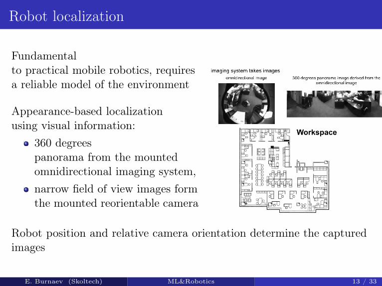
Fundamentalto practical mobile robotics, requiresa reliable model of the environment
Appearance-based localizationusing visual information:
360 degreespanorama from the mountedomnidirectional imaging system,narrow field of view images formthe mounted reorientable camera
Robot position and relative camera orientation determine the capturedimages
E. Burnaev (Skoltech) ML&Robotics 13 / 33
Regression on images
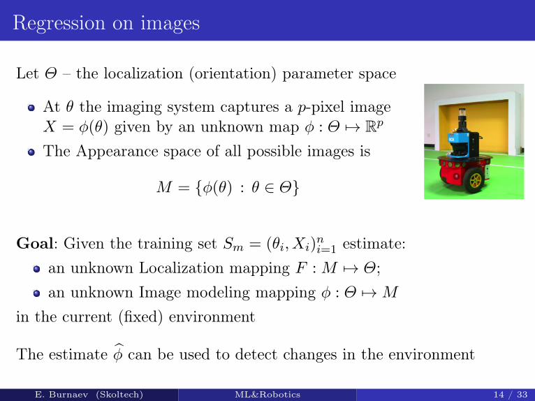
Let Θ – the localization (orientation) parameter space
At θ the imaging system captures a p-pixel imageX = φ(θ) given by an unknown map φ : Θ 7→ Rp
The Appearance space of all possible images is
M = {φ(θ) : θ ∈ Θ}
Goal: Given the training set Sm = (θi, Xi)ni=1 estimate:
an unknown Localization mapping F :M 7→ Θ;an unknown Image modeling mapping φ : Θ 7→M
in the current (fixed) environment
The estimate φ can be used to detect changes in the environment
E. Burnaev (Skoltech) ML&Robotics 14 / 33
Regression on images
The Localization mapping F , and the Image modeling mapping φ sufferfrom the “curse of dimensionality”:
instability due to collinearity or “near-collinearity” of p-dimensionalinputs;regression error can not tend to zero faster than O(n−
s2s+p ) when
an unknown function is at least s times differentiable
E. Burnaev (Skoltech) ML&Robotics 15 / 33
Regression on Image Manifold
The Appearance space
M = {φ(θ) : θ ∈ Θ ⊂ Rq} ⊂ Rp ,
is a low-dimensional manifold (Appearance manifold) with smallintrinsic dimension q embedded in p-dimensional Euclidean space andcovered by a single chart φ
Manifold nature of the input space avoids the curse of dimensionality
E. Burnaev (Skoltech) ML&Robotics 16 / 33
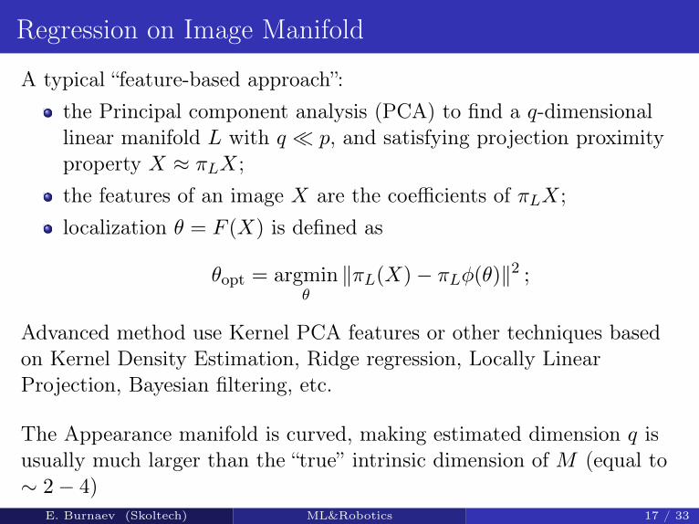
Regression on Image Manifold
A typical “feature-based approach”:the Principal component analysis (PCA) to find a q-dimensionallinear manifold L with q � p, and satisfying projection proximityproperty X ≈ πLX;the features of an image X are the coefficients of πLX;localization θ = F (X) is defined as
θopt = argminθ‖πL(X)− πLφ(θ)‖2 ;
Advanced method use Kernel PCA features or other techniques basedon Kernel Density Estimation, Ridge regression, Locally LinearProjection, Bayesian filtering, etc.
The Appearance manifold is curved, making estimated dimension q isusually much larger than the “true” intrinsic dimension of M (equal to∼ 2− 4)
E. Burnaev (Skoltech) ML&Robotics 17 / 33
1 Predictive Modelling in Industrial EngineeringPredictive ModellingCustomer ExpectationsSurrogate ModelsDimension Reduction
2 Robot navigation
3 ML problem statement
4 Robot control
5 Conclusions
E. Burnaev (Skoltech) ML&Robotics 18 / 33
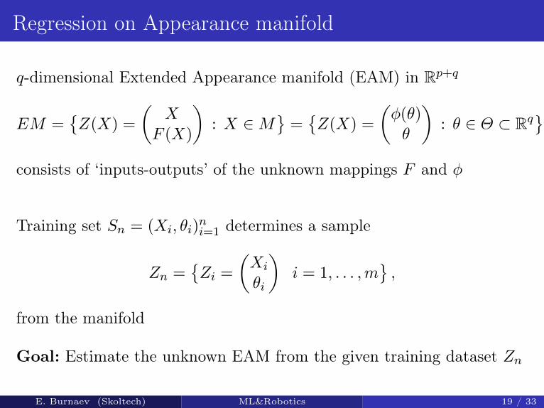
Regression on Appearance manifold
q-dimensional Extended Appearance manifold (EAM) in Rp+q
EM ={Z(X) =
(X
F (X)
): X ∈M
}={Z(X) =
(φ(θ)θ
): θ ∈ Θ ⊂ Rq
},
consists of ‘inputs-outputs’ of the unknown mappings F and φ
Training set Sn = (Xi, θi)ni=1 determines a sample
Zn ={Zi =
(Xi
θi
)i = 1, . . . ,m
},
from the manifold
Goal: Estimate the unknown EAM from the given training dataset Zn
E. Burnaev (Skoltech) ML&Robotics 19 / 33
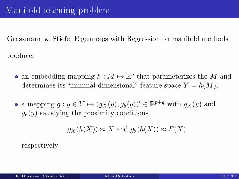
Manifold learning problem
Grassmann & Stiefel Eigenmaps with Regression on manifold methods
produce:
an embedding mapping h :M 7→ Rq that parameterizes the M anddetermines its “minimal-dimensional” feature space Y = h(M);
a mapping g : y ∈ Y 7→ (gX(y), gθ(y))′ ∈ Rp+q with gX(y) and
gθ(y) satisfying the proximity conditions
gX(h(X)) ≈ X and gθ(h(X)) ≈ F (X)
respectively
E. Burnaev (Skoltech) ML&Robotics 20 / 33
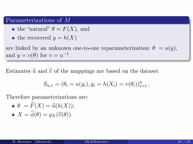
Parameterizations of Mthe “natural” θ = F (X), andthe recovered y = h(X)
are linked by an unknown one-to-one reparameterization: θ = u(y),and y = v(θ) for v = u−1.
Estimates u and v of the mappings are based on the dataset
Su,v = (θi = u(yi), yi = h(Xi) = v(θi))ni=1 .
Therefore parameterizations are:θ = F (X) = u(h(X));X = φ(θ) = gX(v(θ)).
E. Burnaev (Skoltech) ML&Robotics 21 / 33
1 Predictive Modelling in Industrial EngineeringPredictive ModellingCustomer ExpectationsSurrogate ModelsDimension Reduction
2 Robot navigation
3 ML problem statement
4 Robot control
5 Conclusions
E. Burnaev (Skoltech) ML&Robotics 22 / 33
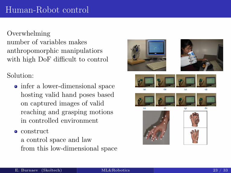
Human-Robot control
Overwhelmingnumber of variables makesanthropomorphic manipulatiorswith high DoF difficult to control
Solution:infer a lower-dimensional spacehosting valid hand poses basedon captured images of validreaching and grasping motionsin controlled environmentconstructa control space and lawfrom this low-dimensional space
E. Burnaev (Skoltech) ML&Robotics 23 / 33
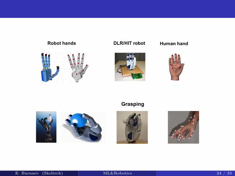
E. Burnaev (Skoltech) ML&Robotics 24 / 33
Manifold learning approach
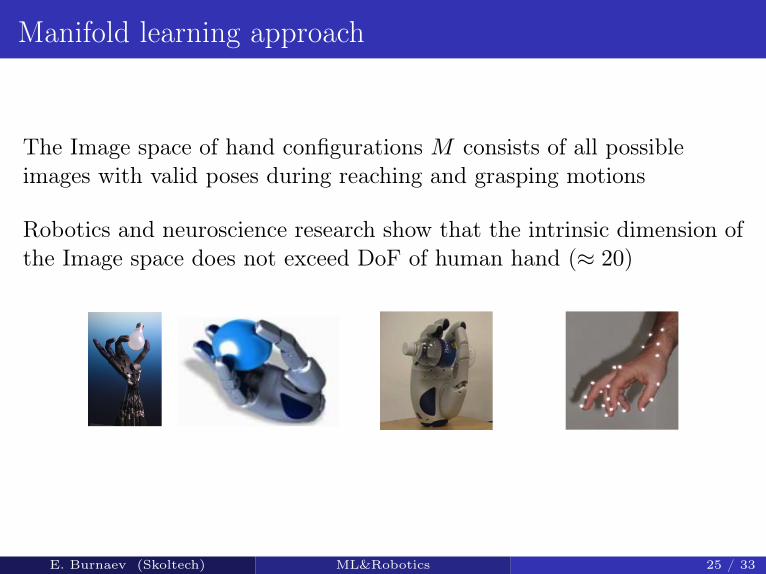
The Image space of hand configurations M consists of all possibleimages with valid poses during reaching and grasping motions
Robotics and neuroscience research show that the intrinsic dimension ofthe Image space does not exceed DoF of human hand (≈ 20)
E. Burnaev (Skoltech) ML&Robotics 25 / 33
Low-dimensional image features in Human hand poses
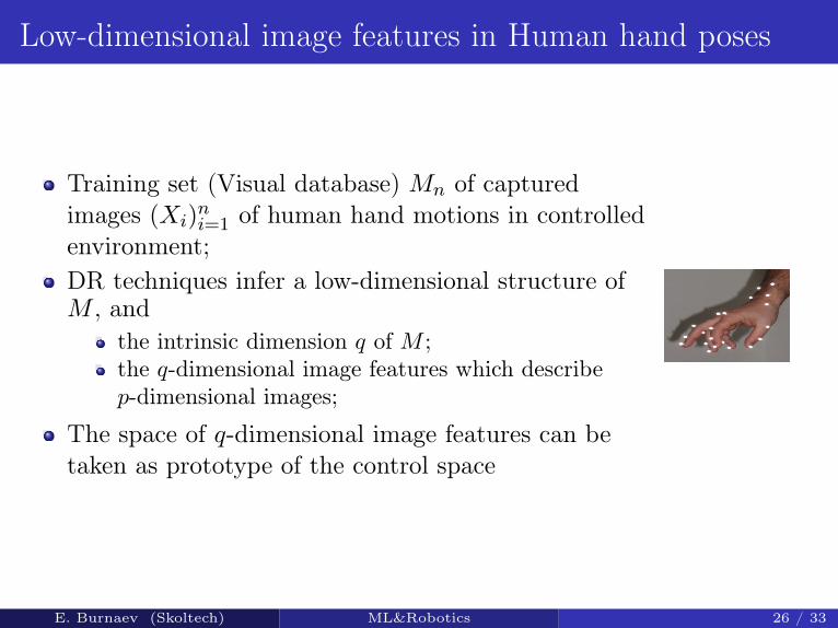
Training set (Visual database) Mn of capturedimages (Xi)
ni=1 of human hand motions in controlled
environment;DR techniques infer a low-dimensional structure ofM , and
the intrinsic dimension q of M ;the q-dimensional image features which describep-dimensional images;
The space of q-dimensional image features can betaken as prototype of the control space
E. Burnaev (Skoltech) ML&Robotics 26 / 33
Low-dimensional image features in Human hand poses
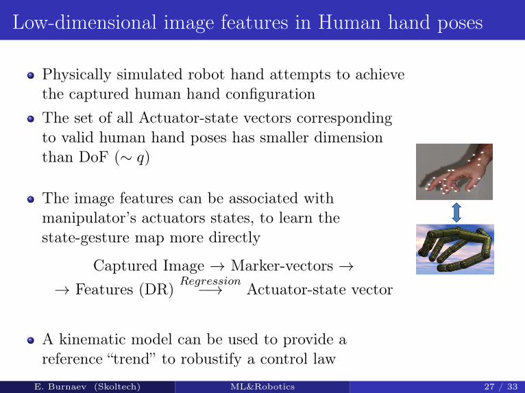
Physically simulated robot hand attempts to achievethe captured human hand configurationThe set of all Actuator-state vectors correspondingto valid human hand poses has smaller dimensionthan DoF (∼ q)
The image features can be associated withmanipulator’s actuators states, to learn thestate-gesture map more directly
Captured Image → Marker-vectors →→ Features (DR) Regression−→ Actuator-state vector
A kinematic model can be used to provide areference “trend” to robustify a control law
E. Burnaev (Skoltech) ML&Robotics 27 / 33
Eigengrasps
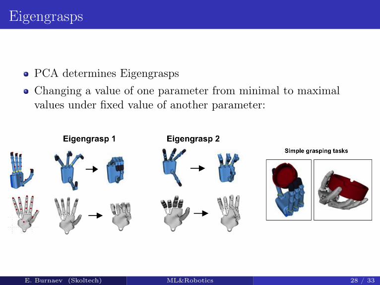
PCA determines EigengraspsChanging a value of one parameter from minimal to maximalvalues under fixed value of another parameter:
E. Burnaev (Skoltech) ML&Robotics 28 / 33
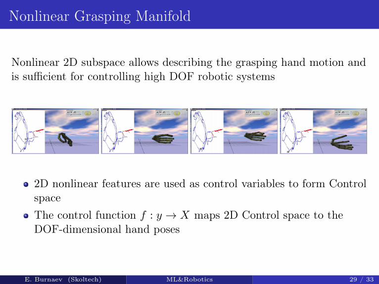
Nonlinear Grasping Manifold
Nonlinear 2D subspace allows describing the grasping hand motion andis sufficient for controlling high DOF robotic systems
2D nonlinear features are used as control variables to form ControlspaceThe control function f : y → X maps 2D Control space to theDOF-dimensional hand poses
E. Burnaev (Skoltech) ML&Robotics 29 / 33
1 Predictive Modelling in Industrial EngineeringPredictive ModellingCustomer ExpectationsSurrogate ModelsDimension Reduction
2 Robot navigation
3 ML problem statement
4 Robot control
5 Conclusions
E. Burnaev (Skoltech) ML&Robotics 30 / 33
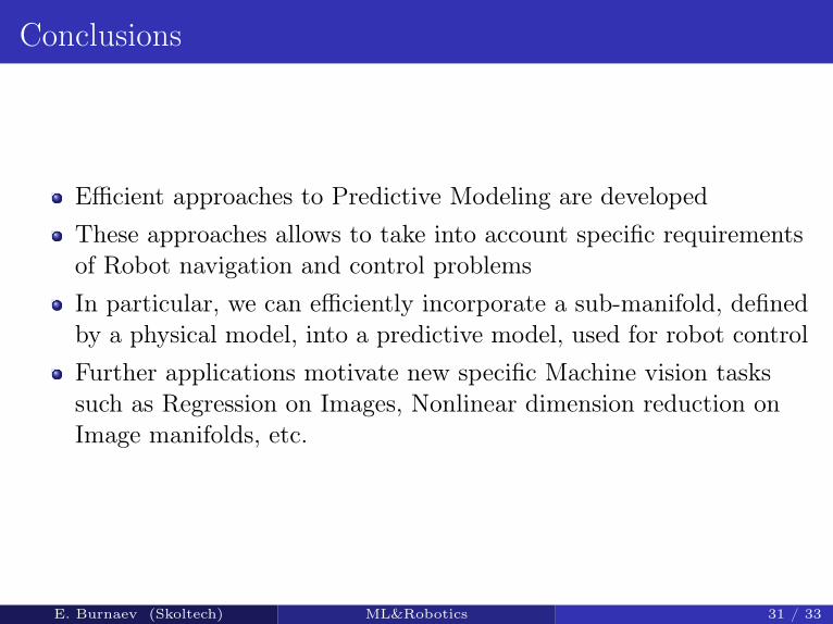
Conclusions
Efficient approaches to Predictive Modeling are developedThese approaches allows to take into account specific requirementsof Robot navigation and control problemsIn particular, we can efficiently incorporate a sub-manifold, definedby a physical model, into a predictive model, used for robot controlFurther applications motivate new specific Machine vision taskssuch as Regression on Images, Nonlinear dimension reduction onImage manifolds, etc.
E. Burnaev (Skoltech) ML&Robotics 31 / 33

E. Burnaev (Skoltech) ML&Robotics 32 / 33
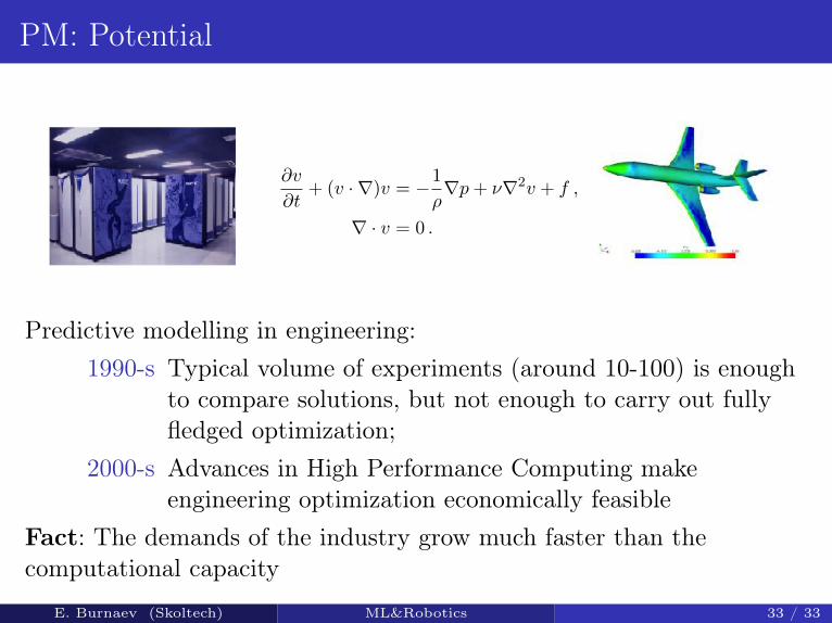
PM: Potential
∂v
∂t+ (v · ∇)v = −1
ρ∇p+ ν∇2v + f ,
∇ · v = 0 .
Predictive modelling in engineering:1990-s Typical volume of experiments (around 10-100) is enough
to compare solutions, but not enough to carry out fullyfledged optimization;
2000-s Advances in High Performance Computing makeengineering optimization economically feasible
Fact: The demands of the industry grow much faster than thecomputational capacity
E. Burnaev (Skoltech) ML&Robotics 33 / 33