Keywords： • OpenFOAM • fvOptions

Fumiya Nozaki

最終更新日: 2014年6月29日

日本語版

OpenFOAM

壁関数

Wall Functions

2

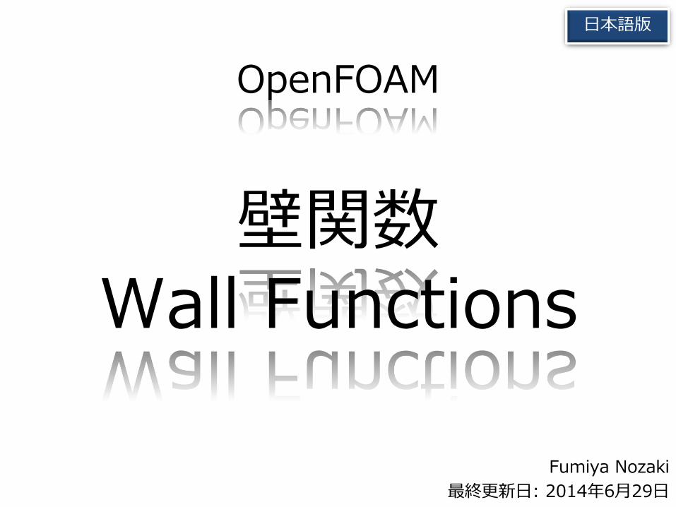
渦粘性係数用の境界条件

非圧縮性流れの解析では，渦粘性係数 𝜈𝑡 (OpenFOAMでは “nut” と表記) の境界条件として以下のものが使用できます．

ソースコードの場所 src/turbulenceModels/incompressible /RAS/derivedFvPatchFields /wallFunctions/nutWallFunctions 名前に “Rough” と付いているものは，

壁面粗さを考慮した計算用です．

3

Chapter 1. nutkWallFunction

4

壁面上の渦粘性係数の計算

tmp<scalarField> nutkWallFunctionFvPatchScalarField::calcNut() const

{

const label patchi = patch().index();

const turbulenceModel& turbModel =

db().lookupObject<turbulenceModel>("turbulenceModel");

const scalarField& y = turbModel.y()[patchi];

const tmp<volScalarField> tk = turbModel.k();

const volScalarField& k = tk();

const tmp<volScalarField> tnu = turbModel.nu();

const volScalarField& nu = tnu();

const scalarField& nuw = nu.boundaryField()[patchi];

const scalar Cmu25 = pow025(Cmu_);

tmp<scalarField> tnutw(new scalarField(patch().size(), 0.0));

scalarField& nutw = tnutw();

forAll(nutw, faceI)

{

label faceCellI = patch().faceCells()[faceI];

scalar yPlus = Cmu25*y[faceI]*sqrt(k[faceCellI])/nuw[faceI];

if (yPlus > yPlusLam_)

{

nutw[faceI] = nuw[faceI]*(yPlus*kappa_/log(E_*yPlus) - 1.0);

}

}

return tnutw;

}

nutw[faceI]は， faceI番目のフェイスでの 渦粘性係数の値です．

nutkWallFunctionFvPatchScalarField.C

5

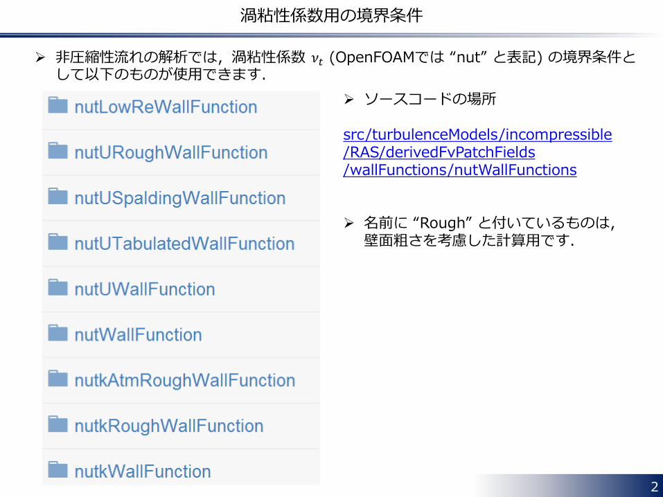
壁面上の渦粘性係数の計算

𝜈𝑡𝑤𝑎𝑙𝑙 = 𝜈

𝜅𝑦+

𝑙𝑜𝑔 𝐸𝑦+− 1

0

𝑦+ > 𝑦𝑙𝑎𝑚

+

𝑦+ ≤ 𝑦𝑙𝑎𝑚+

𝑦+ =𝐶𝜇1 4 𝑦 𝑘

𝜈𝑤

壁面上の渦粘性係数の値を，𝑦+ と 𝑦𝑙𝑎𝑚+ の大小関係により場合分けして計算します．

yPlusLam

𝑦+ > 𝑦𝑙𝑎𝑚+ 𝑦+ ≤ 𝑦𝑙𝑎𝑚

+

6

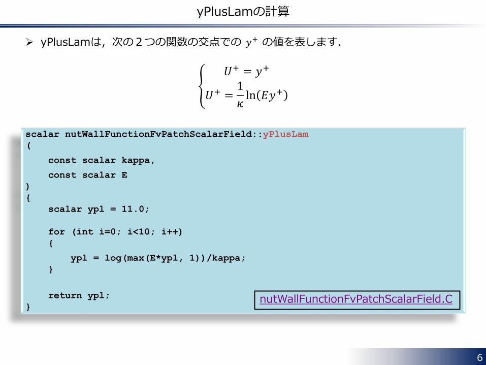
yPlusLamの計算

scalar nutWallFunctionFvPatchScalarField::yPlusLam

(

const scalar kappa,

const scalar E

)

{

scalar ypl = 11.0;

for (int i=0; i<10; i++)

{

ypl = log(max(E*ypl, 1))/kappa;

}

return ypl;

} nutWallFunctionFvPatchScalarField.C

yPlusLamは，次の２つの関数の交点での 𝑦+ の値を表します．

𝑈+ = 𝑦+

𝑈+ =1

𝜅ln 𝐸𝑦+

7

yPlusLamの計算

yPlusLamの値は反復法 [1] により計算しています．

𝐸 = 9.8，𝜅 = 0.41 の場合に実際に計算してみると， • 初期値 ypl = 11 • i=0 ypl = 11.415311362133 • i=1 ypl = 11.505702297229 • i=2 ypl = 11.524939390450 • i=3 ypl = 11.529013940444 • i=4 ypl = 11.529876085585 • i=5 ypl = 11.530058470168 • i=6 ypl = 11.530097051410 • i=7 ypl = 11.530105212724 • i=8 ypl = 11.530106939131 • i=9 ypl = 11.530107304327

小数点以下7桁目まで一致しているのが確認できます．

𝑈+ =1

𝜅𝑙𝑛 𝐸𝑦+ = 11.53010738

8

𝑦 + の計算

tmp<scalarField> nutkWallFunctionFvPatchScalarField::yPlus() const

{

const label patchi = patch().index();

const turbulenceModel& turbModel =

db().lookupObject<turbulenceModel>("turbulenceModel");

const scalarField& y = turbModel.y()[patchi];

const tmp<volScalarField> tk = turbModel.k();

const volScalarField& k = tk();

tmp<scalarField> kwc = k.boundaryField()[patchi].patchInternalField();

const tmp<volScalarField> tnu = turbModel.nu();

const volScalarField& nu = tnu();

const scalarField& nuw = nu.boundaryField()[patchi];

return pow025(Cmu_)*y*sqrt(kwc)/nuw;

}

“yPlusRAS” ユーティリティを使用して，𝑦 + の値を計算する際に，各境界条件で定義されている yPlus() が呼ばれます．

nutkWallFunctionFvPatchScalarField.C

9

yPlusRAS

const volScalarField::GeometricBoundaryField nutPatches =

RASModel->nut()().boundaryField();

bool foundNutPatch = false;

forAll(nutPatches, patchi)

{

if (isA<wallFunctionPatchField>(nutPatches[patchi]))

{

foundNutPatch = true;

const wallFunctionPatchField& nutPw =

dynamic_cast<const wallFunctionPatchField&>

(nutPatches[patchi]);

yPlus.boundaryField()[patchi] = nutPw.yPlus();

const scalarField& Yp = yPlus.boundaryField()[patchi];

Info<< "Patch " << patchi

<< " named " << nutPw.patch().name()

<< " y+ : min: " << gMin(Yp) << " max: " << gMax(Yp)

<< " average: " << gAverage(Yp) << nl << endl;

}

}

yPlusRAS.C

ここから呼ばれます．

10

Chapter 2. nutUSpaldingWallFunction

11

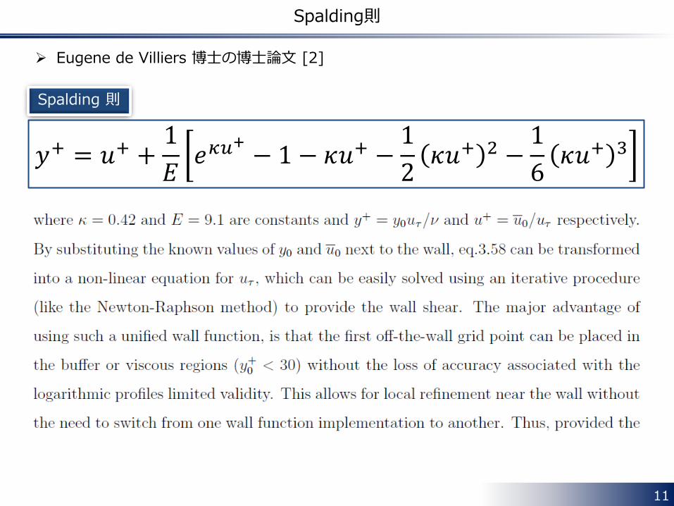
Spalding則

𝑦+ = 𝑢+ +1

𝐸𝑒𝜅𝑢

+− 1 − 𝜅𝑢+ −

1

2𝜅𝑢+ 2 −

1

6𝜅𝑢+ 3

Eugene de Villiers 博士の博士論文 [2]

Spalding 則

12

Spalding則

この 𝑦+ と 𝑢+ の関係式は，粘性底層での関係式 𝑢+ = 𝑦+ と対数則領域での関係式

𝑢+ =1

𝜅ln 𝐸𝑦+ をうまくフィッテイングした関数です．

𝑦+

𝑢+

Spalding 則

𝑢+ = 𝑦+

𝑢+ =1

𝜅ln 𝐸𝑦+

13

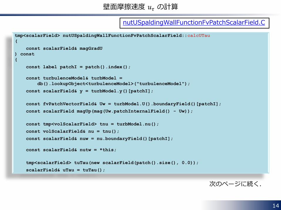
壁面上の渦粘性係数の計算

tmp<scalarField> nutUSpaldingWallFunctionFvPatchScalarField::calcNut() const

{

const label patchI = patch().index();

const turbulenceModel& turbModel =

db().lookupObject<turbulenceModel>("turbulenceModel");

const fvPatchVectorField& Uw = turbModel.U().boundaryField()[patchI];

const scalarField magGradU(mag(Uw.snGrad()));

const tmp<volScalarField> tnu = turbModel.nu();

const volScalarField& nu = tnu();

const scalarField& nuw = nu.boundaryField()[patchI];

return max

(

scalar(0),

sqr(calcUTau(magGradU))/(magGradU + ROOTVSMALL) - nuw

);

}

𝜈𝑡𝑤𝑎𝑙𝑙 =𝑢𝜏2

𝜕𝒖𝜕𝒏

− 𝜈

nutUSpaldingWallFunctionFvPatchScalarField.C

壁面摩擦速度 𝑢𝜏 を Spalding則 から計算します．

14

壁面摩擦速度 𝑢𝜏 の計算

tmp<scalarField> nutUSpaldingWallFunctionFvPatchScalarField::calcUTau

(

const scalarField& magGradU

) const

{

const label patchI = patch().index();

const turbulenceModel& turbModel =

db().lookupObject<turbulenceModel>("turbulenceModel");

const scalarField& y = turbModel.y()[patchI];

const fvPatchVectorField& Uw = turbModel.U().boundaryField()[patchI];

const scalarField magUp(mag(Uw.patchInternalField() - Uw));

const tmp<volScalarField> tnu = turbModel.nu();

const volScalarField& nu = tnu();

const scalarField& nuw = nu.boundaryField()[patchI];

const scalarField& nutw = *this;

tmp<scalarField> tuTau(new scalarField(patch().size(), 0.0));

scalarField& uTau = tuTau();

nutUSpaldingWallFunctionFvPatchScalarField.C

次のページに続く．

15

壁面摩擦速度 𝑢𝜏 の計算

forAll(uTau, faceI)

{

scalar ut = sqrt((nutw[faceI] + nuw[faceI])*magGradU[faceI]);

if (ut > ROOTVSMALL)

{

int iter = 0;

scalar err = GREAT;

do

{

scalar kUu = min(kappa_*magUp[faceI]/ut, 50);

scalar fkUu = exp(kUu) - 1 - kUu*(1 + 0.5*kUu);

scalar f =

- ut*y[faceI]/nuw[faceI]

+ magUp[faceI]/ut

+ 1/E_*(fkUu - 1.0/6.0*kUu*sqr(kUu));

scalar df =

y[faceI]/nuw[faceI]

+ magUp[faceI]/sqr(ut)

+ 1/E_*kUu*fkUu/ut;

scalar uTauNew = ut + f/df;

err = mag((ut - uTauNew)/ut);

ut = uTauNew;

} while (ut > ROOTVSMALL && err > 0.01 && ++iter < 10);

uTau[faceI] = max(0.0, ut);

}

}

Newton-Raphson法を 使用して壁面摩擦速度 𝑢𝜏 を反復計算で求めています．

漸化式

反復継続条件

nutUSpaldingWallFunctionFvPatchScalarField.C

16

壁面摩擦速度 𝑢𝜏 の計算

calcUTau() では，Spalding則を満たす 𝑢𝜏 を Newton-Raphson法により求めます．

𝑓 𝑢𝜏, 𝑦, 𝑢 = −𝑦+ + 𝑢+ +1

𝐸𝑒𝜅𝑢

+− 1 − 𝜅𝑢+ −

1

2𝜅𝑢+ 2 −

1

6𝜅𝑢+ 3 = 0

Newton-Raphsonの漸化式

𝑢𝜏𝑛+1 = 𝑢𝜏

𝑛 −𝑓 𝑢𝜏

𝑛, 𝑦, 𝑢

𝑓′ 𝑢𝜏𝑛, 𝑦, 𝑢

壁面隣接セル中心における

• 𝑦 の値，つまり壁面からの距離と • 各時間ステップでの流速 𝑢

が既知なので，ただ１つの未知数である 𝑢𝜏 について解くことができます．

ソースコードの中では -df

17

𝑦 + の計算

tmp<scalarField> nutUSpaldingWallFunctionFvPatchScalarField::yPlus() const

{

const label patchi = patch().index();

const turbulenceModel& turbModel =

db().lookupObject<turbulenceModel>("turbulenceModel");

const scalarField& y = turbModel.y()[patchi];

const fvPatchVectorField& Uw = turbModel.U().boundaryField()[patchi];

const tmp<volScalarField> tnu = turbModel.nu();

const volScalarField& nu = tnu();

const scalarField& nuw = nu.boundaryField()[patchi];

return y*calcUTau(mag(Uw.snGrad()))/nuw;

}

nutUSpaldingWallFunctionFvPatchScalarField.C

18

Chapter 3. nutLowReWallFunction

19

壁面上の渦粘性係数の計算

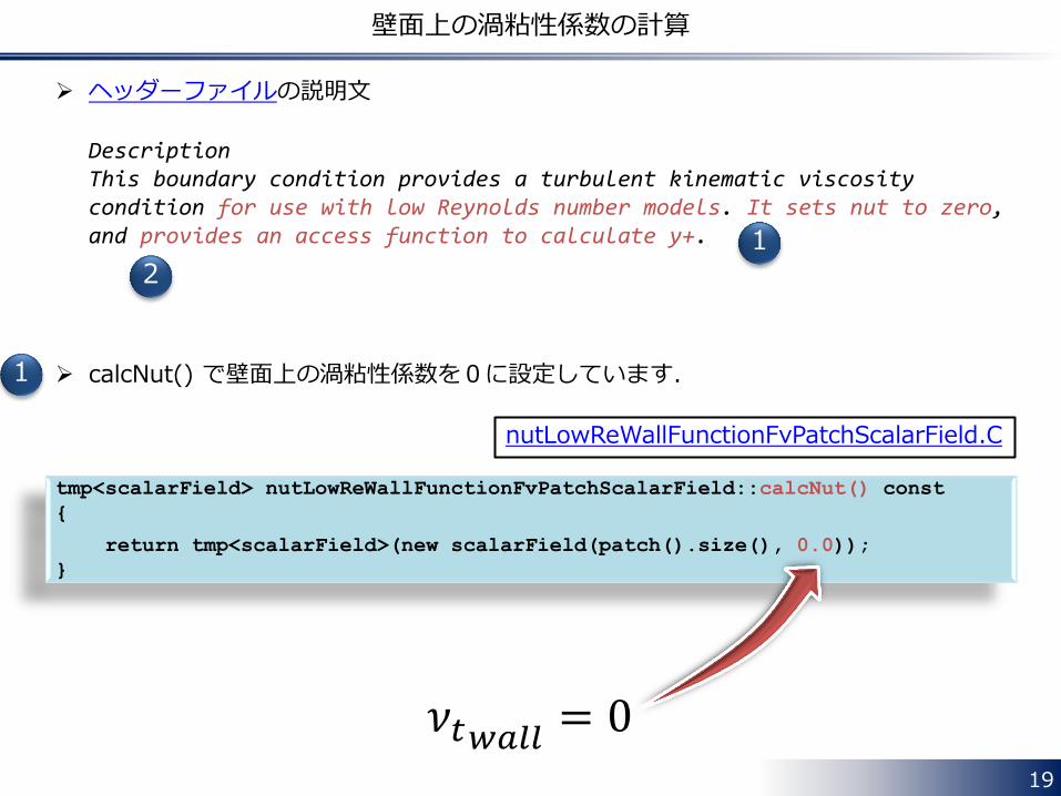
tmp<scalarField> nutLowReWallFunctionFvPatchScalarField::calcNut() const

{

return tmp<scalarField>(new scalarField(patch().size(), 0.0));

}

nutLowReWallFunctionFvPatchScalarField.C

ヘッダーファイルの説明文

Description This boundary condition provides a turbulent kinematic viscosity condition for use with low Reynolds number models. It sets nut to zero, and provides an access function to calculate y+.

calcNut() で壁面上の渦粘性係数を０に設定しています．

𝜈𝑡𝑤𝑎𝑙𝑙 = 0

1

2

1

20

𝑦 + の計算

tmp<scalarField> nutLowReWallFunctionFvPatchScalarField::yPlus() const

{

const label patchi = patch().index();

const turbulenceModel& turbModel =

db().lookupObject<turbulenceModel>("turbulenceModel");

const scalarField& y = turbModel.y()[patchi];

const tmp<volScalarField> tnu = turbModel.nu();

const volScalarField& nu = tnu();

const scalarField& nuw = nu.boundaryField()[patchi];

const fvPatchVectorField& Uw = turbModel.U().boundaryField()[patchi];

return y*sqrt(nuw*mag(Uw.snGrad()))/nuw;

}

nutLowReWallFunctionFvPatchScalarField.C

前のスライドで見たように，“fixedValue” 条件で nut の値を 0 に規定した場合と同じ計算になります．

１つの違いは，”nutLowReWallFunction” 条件を使用した場合には，”yPlusRAS” ユーティリティを使って 𝑦+ の値を計算できる点です．

2

𝑦+ =𝑦 𝑢𝜏𝜈

=𝑦 𝜏𝑤 𝜌

𝜈=𝑦 𝜈 𝜕𝒖 𝜕𝒏 𝑤𝑎𝑙𝑙

𝜈

21

参考資料

[1] http://www.index-press.co.jp/books/excel/ex-nv06.pdf [2] http://powerlab.fsb.hr/ped/kturbo/OpenFOAM/docs/EugeneDeVilliersPhD2006.pdf

22

Thank You!