생물공정모사 및 최적화

Biological process simulation and optimization

Major: Interdisciplinary program of the integrated biotechnology

Graduate school of bio- & information technology

Youngil Lim (N110), Lab. FACSYoungil Lim (N110), Lab. FACSphone: +82 31 670 5200 (secretary), +82 31 670 5207 (direct)phone: +82 31 670 5200 (secretary), +82 31 670 5207 (direct)

Fax: +82 31 670 5445, mobile phone: +82 10 7665 5207Fax: +82 31 670 5445, mobile phone: +82 10 7665 5207Email: Email: limyi@hknu.ac.kr, homepage: , homepage: http://hknu.ac.kr/~limyi/index.htm

Part I. Problem Formulation

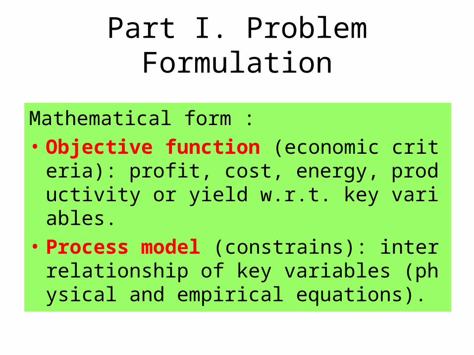
Mathematical form :

• Objective function (economic criteria): profit, cost, energy, productivity or yield w.r.t. key variables.

• Process model (constrains): interrelationship of key variables (physical and empirical equations).

Part I. Problem Formulation

• Ch. 1: Examples in chemical engineering

• Ch. 2: Process models: material/energy balances, equilibrium equations, empirical equations.

• Ch. 3 Objective functions: capital cost/operating cost,

Ch 1. Nature of optimization problems

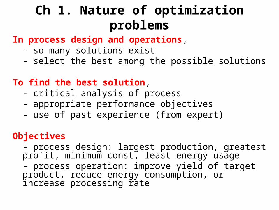
In process design and operations,- so many solutions exist- select the best among the possible solutions

To find the best solution,- critical analysis of process- appropriate performance objectives- use of past experience (from expert)

Objectives- process design: largest production, greatest profit, minimum const, least energy usage- process operation: improve yield of target product, reduce energy consumption, or increase processing rate

Ch 1. Nature of optimization problems

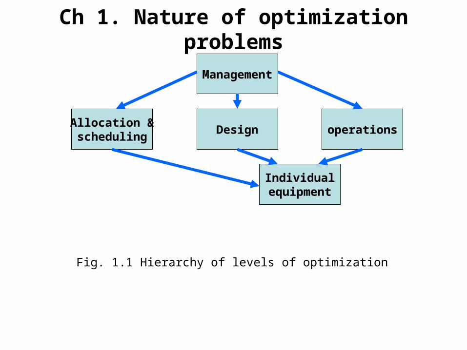
Fig. 1.1 Hierarchy of levels of optimization

Management

Design operationsAllocation &scheduling

Individualequipment

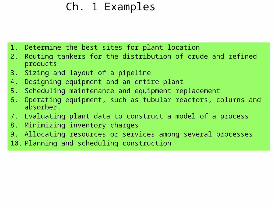
Ch. 1 Examples

1. Determine the best sites for plant location2. Routing tankers for the distribution of crude and refined products3. Sizing and layout of a pipeline4. Designing equipment and an entire plant5. Scheduling maintenance and equipment replacement6. Operating equipment, such as tubular reactors, columns and absorber.7. Evaluating plant data to construct a model of a process8. Minimizing inventory charges9. Allocating resources or services among several processes10. Planning and scheduling construction

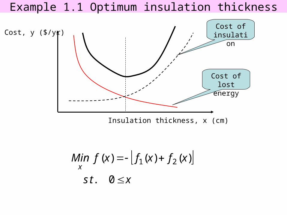
Example 1.1 Optimum insulation thickness

xts

xfxfxfMinx

0..

)()()( 21

Insulation thickness, x (cm)

Cost, y ($/yr)

Cost of lost energy

Cost of insulation

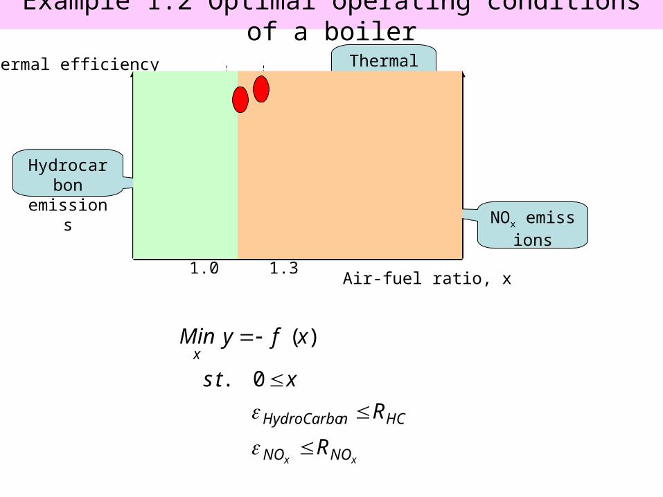
Example 1.2 Optimal operating conditions of a boiler

xx NONO

HCnHydroCarbo

x

R

R

xts

xfyMin

0..

)(

Air-fuel ratio, x

Thermal efficiency

Hydrocarbon emissions

Thermal efficiency

1.0 1.3

NOx emissions

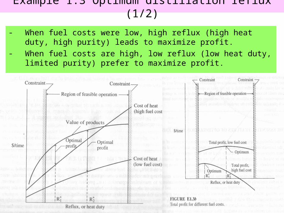
Example 1.3 Optimum distillation reflux (1/2)

- When fuel costs were low, high reflux (high heat duty, high purity) leads to maximize profit.

- When fuel costs are high, low reflux (low heat duty, limited purity) prefer to maximize profit.

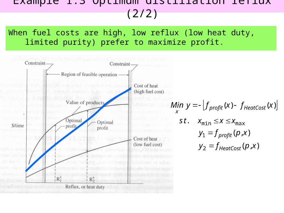
Example 1.3 Optimum distillation reflux (2/2)

),(

),(

..

)()(

2

1

maxmin

xpfy

xpfy

xxxts

xfxfyMin

HeatCost

profit

HeatCostprofitx

When fuel costs are high, low reflux (low heat duty, limited purity) prefer to maximize profit.

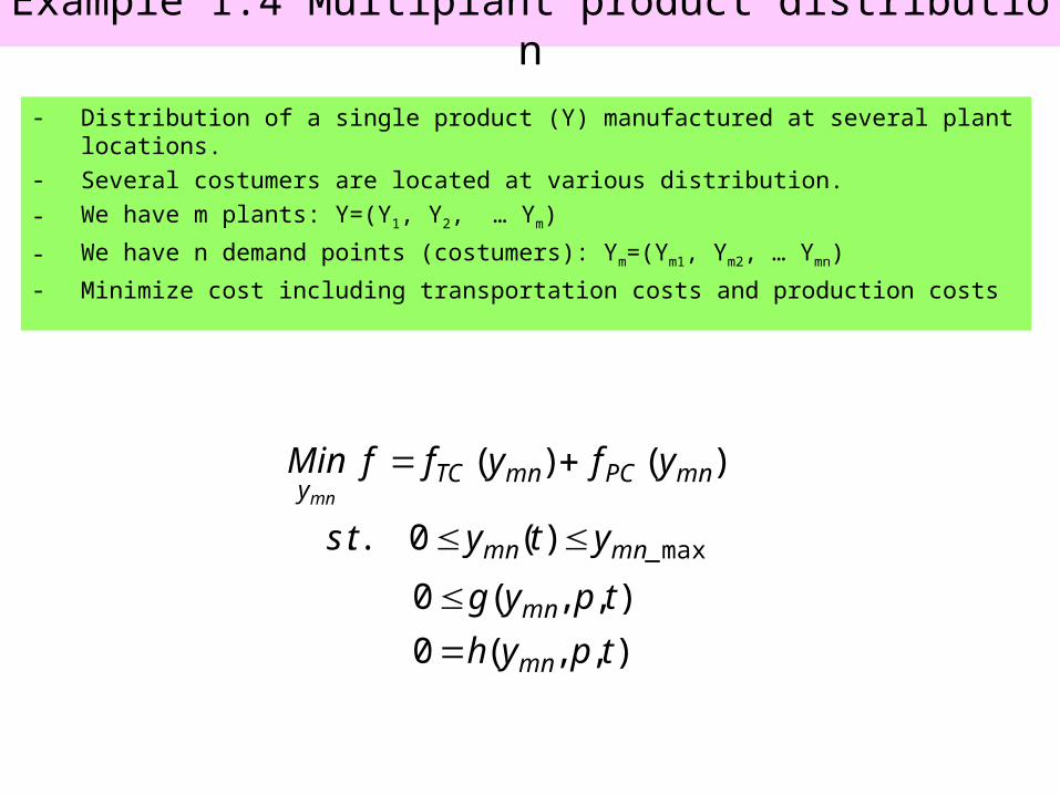
Example 1.4 Multiplant product distribution

),,(0

),,(0

)(0..

)()(

max_

tpyh

tpyg

ytyts

yfyffMin

mn

mn

mnmn

mnPCmnTCymn

- Distribution of a single product (Y) manufactured at several plant locations.

- Several costumers are located at various distribution.

- We have m plants: Y=(Y1, Y2, … Ym)

- We have n demand points (costumers): Ym=(Ym1, Ym2, … Ymn)

- Minimize cost including transportation costs and production costs

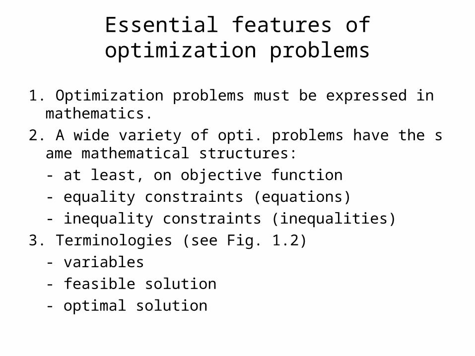
Essential features of optimization problems

1. Optimization problems must be expressed in mathematics.

2. A wide variety of opti. problems have the same mathematical structures:

- at least, on objective function

- equality constraints (equations)

- inequality constraints (inequalities)

3. Terminologies (see Fig. 1.2)

- variables

- feasible solution

- optimal solution

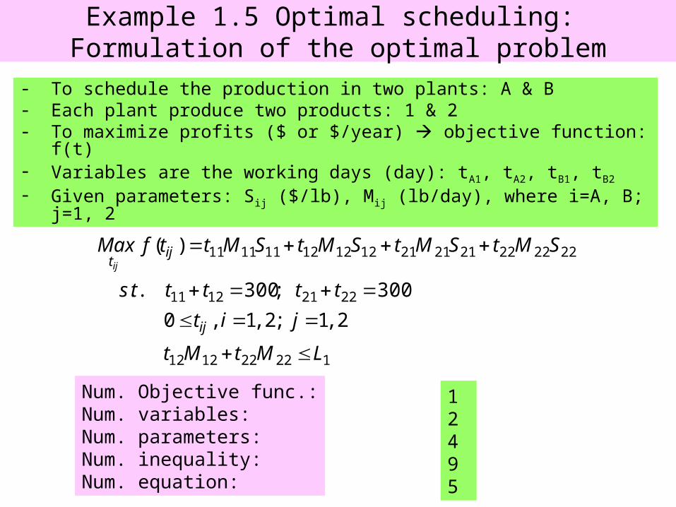
Example 1.5 Optimal scheduling: Formulation of the optimal problem

122221212

22211211

222222212121121212111111

2,1;2,1,0

300;300..

)(

LMtMt

jit

ttttts

SMtSMtSMtSMttfMax

ij

ijtij

- To schedule the production in two plants: A & B- Each plant produce two products: 1 & 2- To maximize profits ($ or $/year) objective function: f(t)- Variables are the working days (day): tA1, tA2, tB1, tB2

- Given parameters: Sij ($/lb), Mij (lb/day), where i=A, B; j=1, 2

Num. Objective func.:Num. variables:Num. parameters:Num. inequality: Num. equation:

124 95

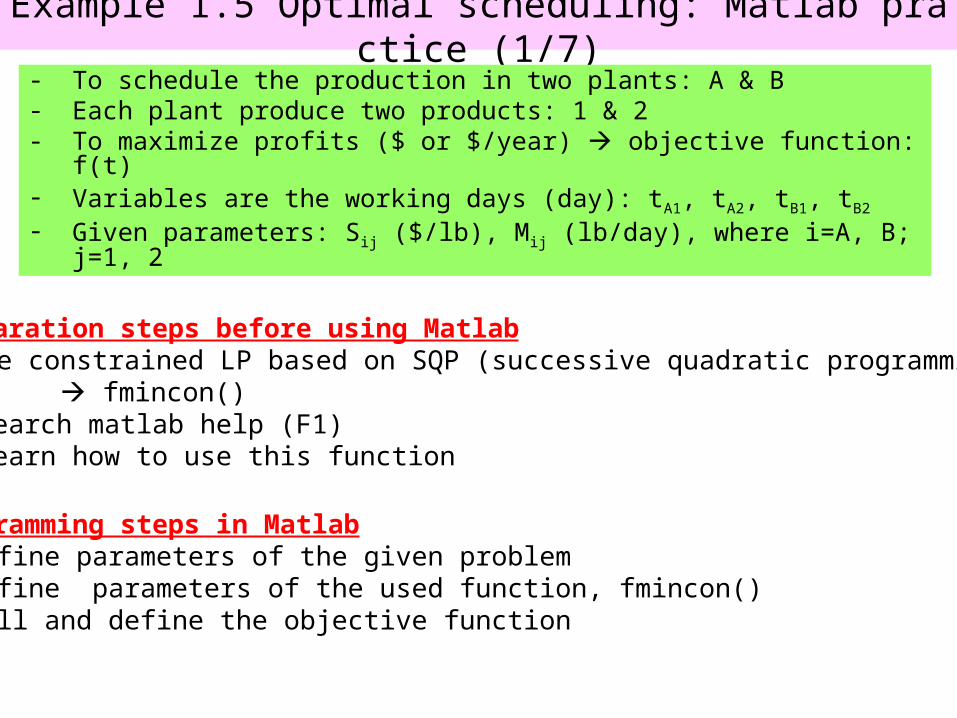
Example 1.5 Optimal scheduling: Matlab practice (1/7)

- To schedule the production in two plants: A & B- Each plant produce two products: 1 & 2- To maximize profits ($ or $/year) objective function: f(t)- Variables are the working days (day): tA1, tA2, tB1, tB2

- Given parameters: Sij ($/lb), Mij (lb/day), where i=A, B; j=1, 2

Preparation steps before using Matlab1. Use constrained LP based on SQP (successive quadratic programming)

fmincon()2. Search matlab help (F1)3. Learn how to use this function

Programming steps in Matlab1. Define parameters of the given problem2. Define parameters of the used function, fmincon()3. Call and define the objective function

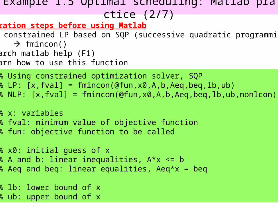
Example 1.5 Optimal scheduling: Matlab practice (2/7)

Preparation steps before using Matlab1. Use constrained LP based on SQP (successive quadratic programming)

fmincon()2. Search matlab help (F1)3. Learn how to use this function

% Using constrained optimization solver, SQP % LP: [x,fval] = fmincon(@fun,x0,A,b,Aeq,beq,lb,ub)% NLP: [x,fval] = fmincon(@fun,x0,A,b,Aeq,beq,lb,ub,nonlcon)

% x: variables% fval: minimum value of objective function% fun: objective function to be called

% x0: initial guess of x% A and b: linear inequalities, A*x <= b% Aeq and beq: linear equalities, Aeq*x = beq

% lb: lower bound of x% ub: upper bound of x

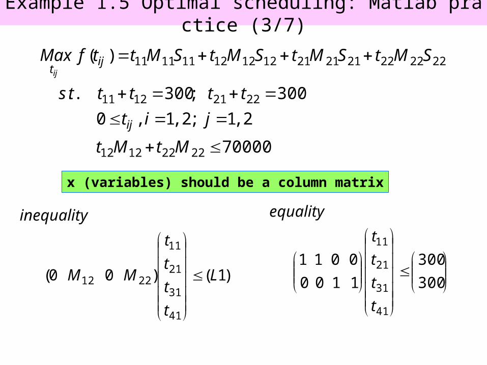
Example 1.5 Optimal scheduling: Matlab practice (3/7)

70000

2,1;2,1,0

300;300..

)(

22221212

22211211

222222212121121212111111

MtMt

jit

ttttts

SMtSMtSMtSMttfMax

ij

ijtij

)1()00(

41

31

21

11

2212 L

t

t

t

t

MM

inequality

300

300

1100

0011

41

31

21

11

t

t

t

t

equality

x (variables) should be a column matrix

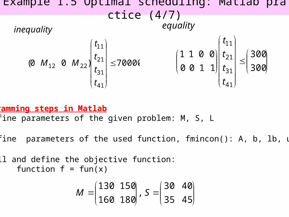
Example 1.5 Optimal scheduling: Matlab practice (4/7)

70000)00(

41

31

21

11

2212

t

t

t

t

MM

inequality

300

300

1100

0011

41

31

21

11

t

t

t

t

equality

Programming steps in Matlab1. Define parameters of the given problem: M, S, L

2. Define parameters of the used function, fmincon(): A, b, lb, ub …

3. Call and define the objective function: function f = fun(x)

4535

4030,

180160

150130SM

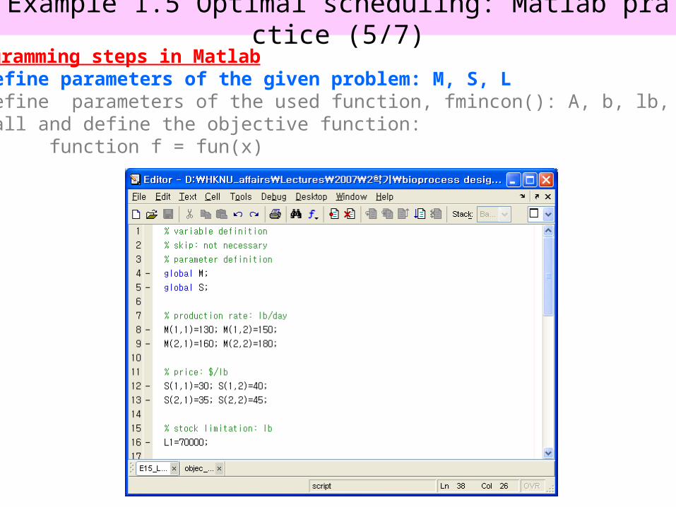
Example 1.5 Optimal scheduling: Matlab practice (5/7)Programming steps in Matlab1. Define parameters of the given problem: M, S, L2. Define parameters of the used function, fmincon(): A, b, lb, ub …3. Call and define the objective function:

function f = fun(x)

Example 1.5 Optimal scheduling: Matlab practice (6/7)

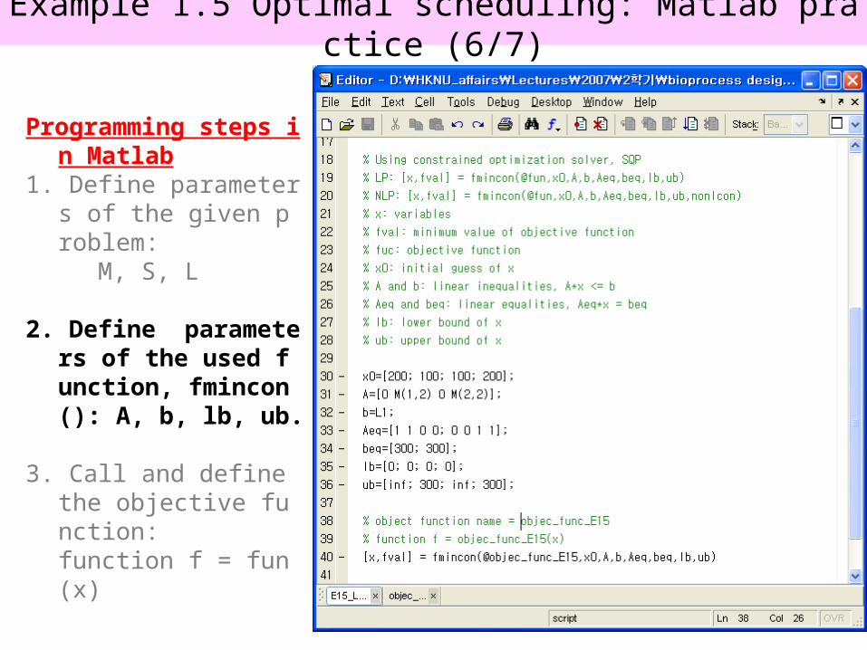
Programming steps in Matlab

1. Define parameters of the given problem:

M, S, L

2. Define parameters of the used function, fmincon(): A, b, lb, ub.

3. Call and define the objective function: function f = fun(x)

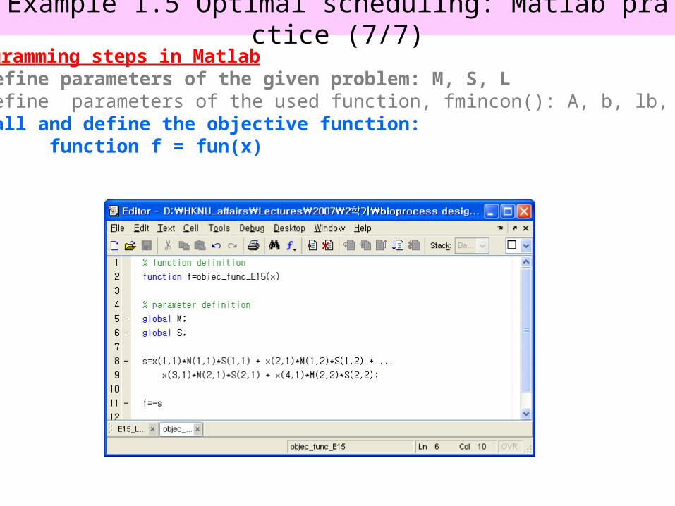
Example 1.5 Optimal scheduling: Matlab practice (7/7)Programming steps in Matlab1. Define parameters of the given problem: M, S, L2. Define parameters of the used function, fmincon(): A, b, lb, ub …3. Call and define the objective function:

function f = fun(x)

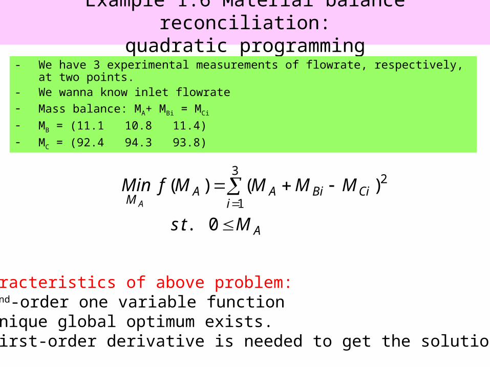
Example 1.6 Material balance reconciliation:quadratic programming

A

iCiBiAA

M

Mts

MMMMfMinA

0..

)()(3

1

2

- We have 3 experimental measurements of flowrate, respectively, at two points.- We wanna know inlet flowrate- Mass balance: MA+ MBi = MCi

- MB = (11.1 10.8 11.4)- MC = (92.4 94.3 93.8)

Characteristics of above problem:1. 2nd-order one variable function2. Unique global optimum exists.3. First-order derivative is needed to get the solution.

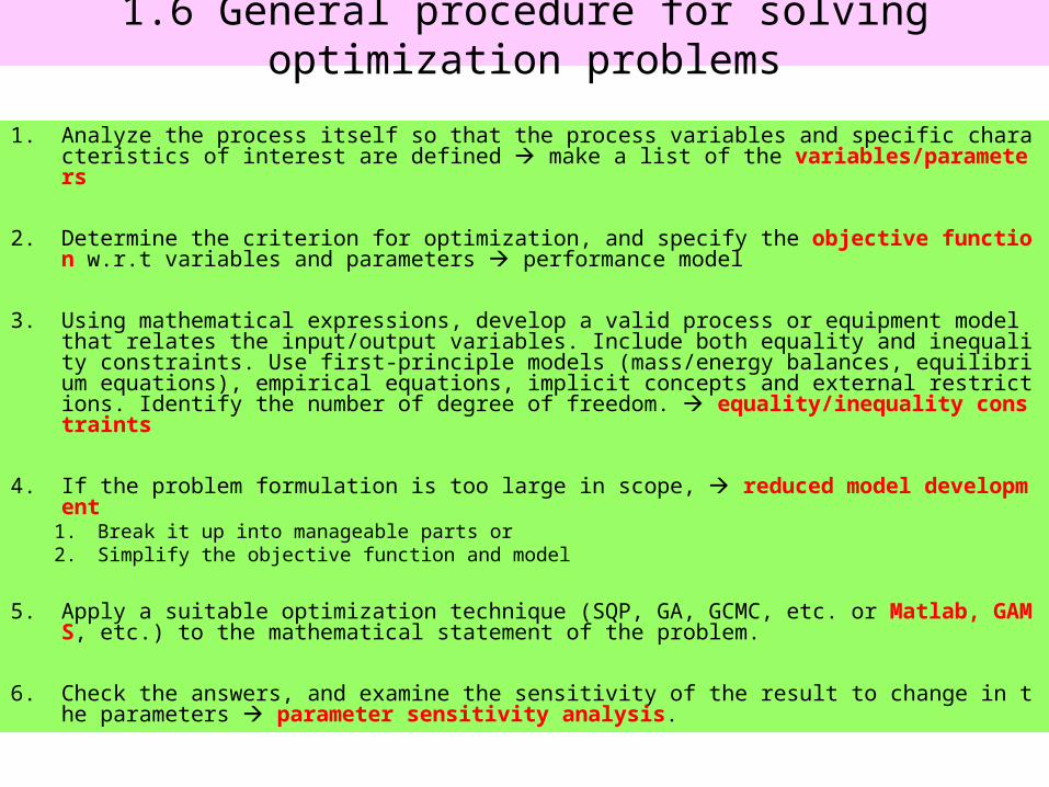
1.6 General procedure for solving optimization problems

1. Analyze the process itself so that the process variables and specific characteristics of interest are defined make a list of the variables/parameters

2. Determine the criterion for optimization, and specify the objective function w.r.t variables and parameters performance model

3. Using mathematical expressions, develop a valid process or equipment model that relates the input/output variables. Include both equality and inequality constraints. Use first-principle models (mass/energy balances, equilibrium equations), empirical equations, implicit concepts and external restrictions. Identify the number of degree of freedom. equality/inequality constraints

4. If the problem formulation is too large in scope, reduced model development1. Break it up into manageable parts or2. Simplify the objective function and model

5. Apply a suitable optimization technique (SQP, GA, GCMC, etc. or Matlab, GAMS, etc.) to the mathematical statement of the problem.

6. Check the answers, and examine the sensitivity of the result to change in the parameters parameter sensitivity analysis.

Exercise and homework 1

• Select one problem among 1.10-1.24 and solve it using Matlab.

• Each student should select a different problem each other.

• If there is no specific value to be needed, please set the values yourself.