Embed Size (px)
DESCRIPTION
統計學 Fall 2003. 授課教師:統計系余清祥 日期:2003年9月30日 第三週:初步資料分析. Chapter 3 Part A Descriptive Statistics: Numerical Methods. Measures of Location Measures of Variability. . . x. %. Measures of Location. Mean Median Mode Percentiles Quartiles. - PowerPoint PPT Presentation
Citation preview
1 1 Slide Slide
統計學 Fall 2003
授課教師:統計系余清祥 日期: 2003 年 9 月 30 日 第三週:初步資料分析
2 2 Slide Slide
Chapter 3 Part AChapter 3 Part A Descriptive Statistics: Numerical Descriptive Statistics: Numerical
MethodsMethods
Measures of LocationMeasures of Location Measures of VariabilityMeasures of Variability
xx
%%
3 3 Slide Slide
Measures of LocationMeasures of Location
MeanMean MedianMedian ModeMode PercentilesPercentiles QuartilesQuartiles
4 4 Slide Slide
Example: Apartment RentsExample: Apartment Rents
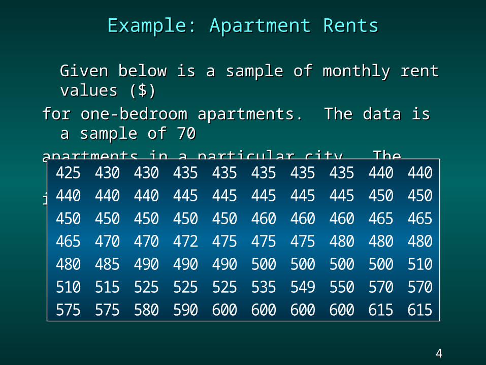
Given below is a sample of monthly rent Given below is a sample of monthly rent values ($)values ($)
for one-bedroom apartments. The data is a for one-bedroom apartments. The data is a sample of 70sample of 70
apartments in a particular city. The data are apartments in a particular city. The data are presentedpresented
in ascending order. in ascending order.
425 430 430 435 435 435 435 435 440 440440 440 440 445 445 445 445 445 450 450450 450 450 450 450 460 460 460 465 465465 470 470 472 475 475 475 480 480 480480 485 490 490 490 500 500 500 500 510510 515 525 525 525 535 549 550 570 570575 575 580 590 600 600 600 600 615 615
425 430 430 435 435 435 435 435 440 440440 440 440 445 445 445 445 445 450 450450 450 450 450 450 460 460 460 465 465465 470 470 472 475 475 475 480 480 480480 485 490 490 490 500 500 500 500 510510 515 525 525 525 535 549 550 570 570575 575 580 590 600 600 600 600 615 615
5 5 Slide Slide
MeanMean
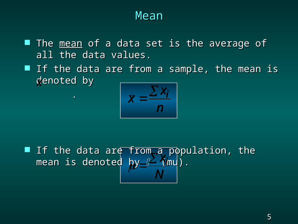
The The meanmean of a data set is the average of all the of a data set is the average of all the data values.data values.
If the data are from a sample, the mean is If the data are from a sample, the mean is denoted by denoted by
..
If the data are from a population, the mean is If the data are from a population, the mean is denoted by denoted by (mu). (mu).
xxnixxni
xNi x
Ni
xx
6 6 Slide Slide
Example: Apartment RentsExample: Apartment Rents
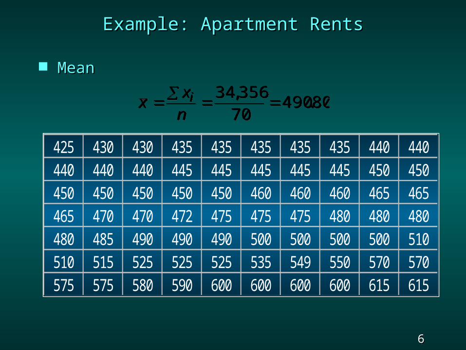
MeanMean
xxni
34 35670
490 80,
.xxni
34 35670
490 80,
.
425 430 430 435 435 435 435 435 440 440440 440 440 445 445 445 445 445 450 450450 450 450 450 450 460 460 460 465 465465 470 470 472 475 475 475 480 480 480480 485 490 490 490 500 500 500 500 510510 515 525 525 525 535 549 550 570 570575 575 580 590 600 600 600 600 615 615
425 430 430 435 435 435 435 435 440 440440 440 440 445 445 445 445 445 450 450450 450 450 450 450 460 460 460 465 465465 470 470 472 475 475 475 480 480 480480 485 490 490 490 500 500 500 500 510510 515 525 525 525 535 549 550 570 570575 575 580 590 600 600 600 600 615 615
7 7 Slide Slide
MedianMedian
The The medianmedian is the measure of location most is the measure of location most often reported for annual income and property often reported for annual income and property value data.value data.
A few extremely large incomes or property A few extremely large incomes or property values can inflate the mean.values can inflate the mean.
8 8 Slide Slide
MedianMedian
The The medianmedian of a data set is the value in the of a data set is the value in the middle when the data items are arranged in middle when the data items are arranged in ascending order.ascending order.
For an odd number of observations, the For an odd number of observations, the median is the middle value.median is the middle value.
For an even number of observations, the For an even number of observations, the median is the average of the two middle median is the average of the two middle values.values.
9 9 Slide Slide
Example: Apartment RentsExample: Apartment Rents
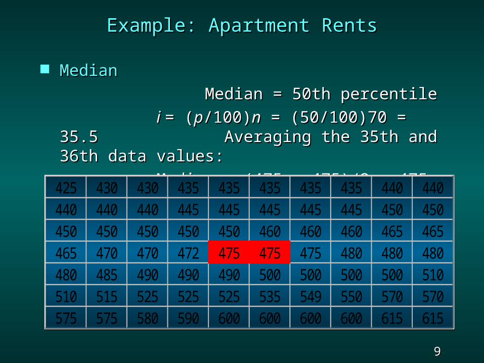
MedianMedian
Median = 50th percentileMedian = 50th percentile
i i = (= (pp/100)/100)nn = (50/100)70 = 35.5 = (50/100)70 = 35.5 Averaging the 35th and Averaging the 35th and
36th data values:36th data values:
Median = (475 + 475)/2 = 475Median = (475 + 475)/2 = 475425 430 430 435 435 435 435 435 440 440440 440 440 445 445 445 445 445 450 450450 450 450 450 450 460 460 460 465 465465 470 470 472 475 475 475 480 480 480480 485 490 490 490 500 500 500 500 510510 515 525 525 525 535 549 550 570 570575 575 580 590 600 600 600 600 615 615
425 430 430 435 435 435 435 435 440 440440 440 440 445 445 445 445 445 450 450450 450 450 450 450 460 460 460 465 465465 470 470 472 475 475 475 480 480 480480 485 490 490 490 500 500 500 500 510510 515 525 525 525 535 549 550 570 570575 575 580 590 600 600 600 600 615 615
10 10 Slide Slide
ModeMode
The The modemode of a data set is the value that occurs of a data set is the value that occurs with greatest frequency.with greatest frequency.
The greatest frequency can occur at two or The greatest frequency can occur at two or more different values.more different values.
If the data have exactly two modes, the data If the data have exactly two modes, the data are are bimodalbimodal..
If the data have more than two modes, the If the data have more than two modes, the data are data are multimodalmultimodal..
11 11 Slide Slide
Example: Apartment RentsExample: Apartment Rents
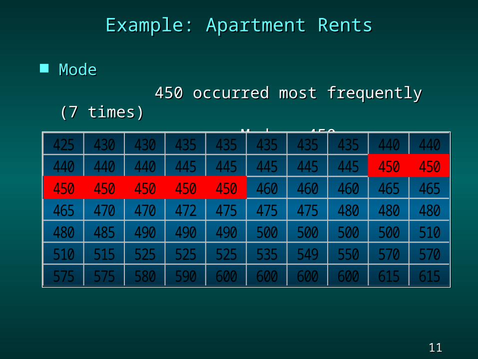
ModeMode
450 occurred most frequently (7 450 occurred most frequently (7 times)times)
Mode = 450Mode = 450425 430 430 435 435 435 435 435 440 440440 440 440 445 445 445 445 445 450 450450 450 450 450 450 460 460 460 465 465465 470 470 472 475 475 475 480 480 480480 485 490 490 490 500 500 500 500 510510 515 525 525 525 535 549 550 570 570575 575 580 590 600 600 600 600 615 615
425 430 430 435 435 435 435 435 440 440440 440 440 445 445 445 445 445 450 450450 450 450 450 450 460 460 460 465 465465 470 470 472 475 475 475 480 480 480480 485 490 490 490 500 500 500 500 510510 515 525 525 525 535 549 550 570 570575 575 580 590 600 600 600 600 615 615
12 12 Slide Slide
PercentilesPercentiles
A percentile provides information about how A percentile provides information about how the data are spread over the interval from the the data are spread over the interval from the smallest value to the largest value.smallest value to the largest value.
Admission test scores for colleges and Admission test scores for colleges and universities are frequently reported in terms of universities are frequently reported in terms of percentiles.percentiles.
13 13 Slide Slide
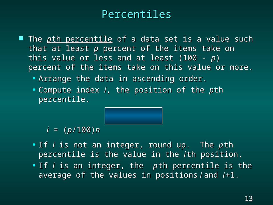
The The ppth percentileth percentile of a data set is a value such that of a data set is a value such that at least at least pp percent of the items take on this value or percent of the items take on this value or less and at least (100 - less and at least (100 - pp) percent of the items take ) percent of the items take on this value or more.on this value or more.
• Arrange the data in ascending order.Arrange the data in ascending order.
• Compute index Compute index ii, the position of the , the position of the ppth th percentile.percentile.
ii = ( = (pp/100)/100)nn
• If If ii is not an integer, round up. The is not an integer, round up. The pp th th percentile is the value in the percentile is the value in the ii th position.th position.
• If If ii is an integer, the is an integer, the pp th percentile is the th percentile is the average of the values in positionsaverage of the values in positions i i and and ii +1.+1.
PercentilesPercentiles
14 14 Slide Slide
Example: Apartment RentsExample: Apartment Rents
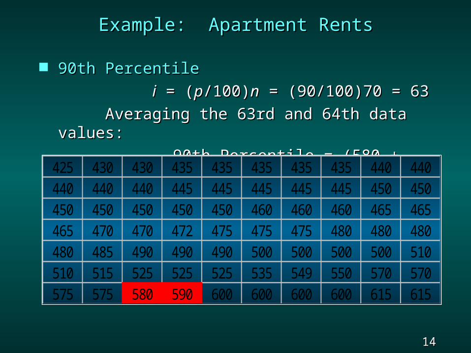
9090th Percentileth Percentile
ii = ( = (pp/100)/100)nn = (90/100)70 = 63 = (90/100)70 = 63
Averaging the 63rd and 64th data Averaging the 63rd and 64th data values:values:
90th Percentile = (580 + 590)/2 = 90th Percentile = (580 + 590)/2 = 585585425 430 430 435 435 435 435 435 440 440
440 440 440 445 445 445 445 445 450 450450 450 450 450 450 460 460 460 465 465465 470 470 472 475 475 475 480 480 480480 485 490 490 490 500 500 500 500 510510 515 525 525 525 535 549 550 570 570575 575 580 590 600 600 600 600 615 615
425 430 430 435 435 435 435 435 440 440440 440 440 445 445 445 445 445 450 450450 450 450 450 450 460 460 460 465 465465 470 470 472 475 475 475 480 480 480480 485 490 490 490 500 500 500 500 510510 515 525 525 525 535 549 550 570 570575 575 580 590 600 600 600 600 615 615
15 15 Slide Slide
QuartilesQuartiles
Quartiles are specific percentilesQuartiles are specific percentiles First Quartile = 25th PercentileFirst Quartile = 25th Percentile Second Quartile = 50th Percentile = MedianSecond Quartile = 50th Percentile = Median Third Quartile = 75th PercentileThird Quartile = 75th Percentile
16 16 Slide Slide
Example: Apartment RentsExample: Apartment Rents
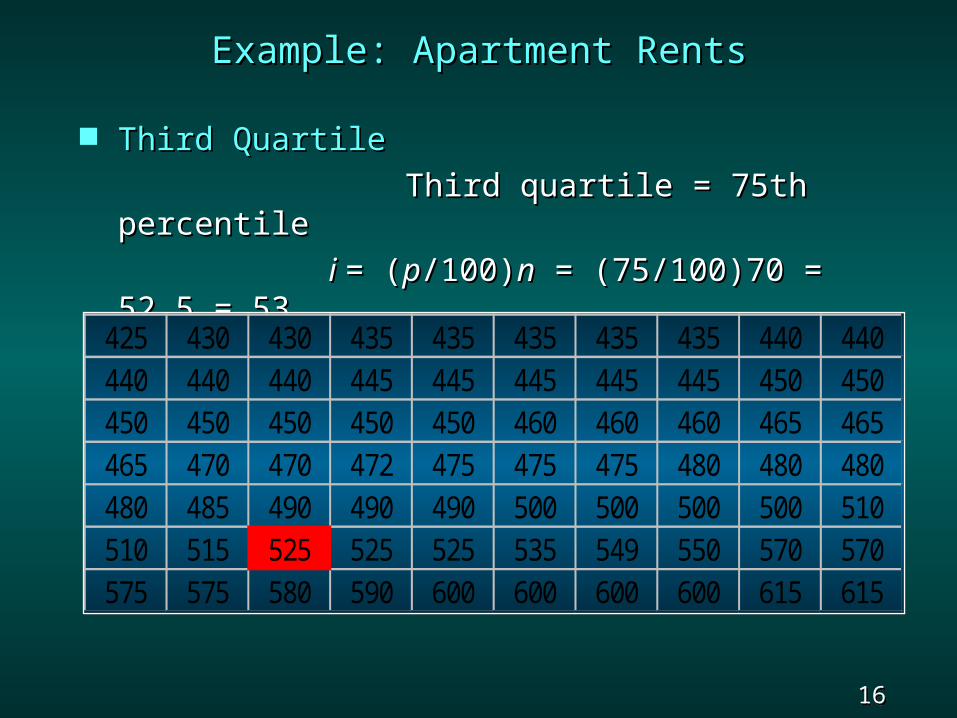
Third QuartileThird Quartile
Third quartile = 75th percentileThird quartile = 75th percentile
i i = (= (pp/100)/100)nn = (75/100)70 = 52.5 = = (75/100)70 = 52.5 = 5353
Third quartile = 525Third quartile = 525425 430 430 435 435 435 435 435 440 440440 440 440 445 445 445 445 445 450 450450 450 450 450 450 460 460 460 465 465465 470 470 472 475 475 475 480 480 480480 485 490 490 490 500 500 500 500 510510 515 525 525 525 535 549 550 570 570575 575 580 590 600 600 600 600 615 615
425 430 430 435 435 435 435 435 440 440440 440 440 445 445 445 445 445 450 450450 450 450 450 450 460 460 460 465 465465 470 470 472 475 475 475 480 480 480480 485 490 490 490 500 500 500 500 510510 515 525 525 525 535 549 550 570 570575 575 580 590 600 600 600 600 615 615

17 17 Slide Slide
Measures of VariabilityMeasures of Variability
It is often desirable to consider measures of It is often desirable to consider measures of variability (dispersion), as well as measures of variability (dispersion), as well as measures of location.location.
For example, in choosing supplier A or supplier For example, in choosing supplier A or supplier B we might consider not only the average B we might consider not only the average delivery time for each, but also the variability delivery time for each, but also the variability in delivery time for each. in delivery time for each.
18 18 Slide Slide
Measures of VariabilityMeasures of Variability
RangeRange Interquartile RangeInterquartile Range VarianceVariance Standard DeviationStandard Deviation Coefficient of VariationCoefficient of Variation
19 19 Slide Slide
RangeRange
The The rangerange of a data set is the difference of a data set is the difference between the largest and smallest data values.between the largest and smallest data values.
It is the It is the simplest measuresimplest measure of variability. of variability. It is It is very sensitivevery sensitive to the smallest and largest to the smallest and largest
data values.data values.
20 20 Slide Slide
Example: Apartment RentsExample: Apartment Rents
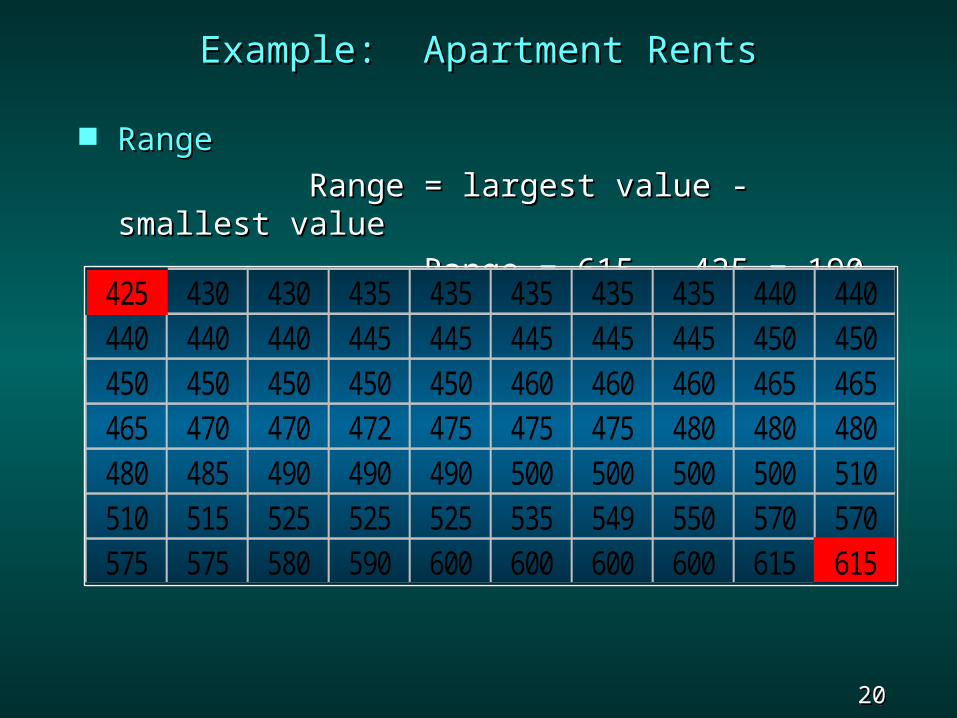
RangeRange
Range = largest value - smallest Range = largest value - smallest value value
Range = 615 - 425 = 190Range = 615 - 425 = 190425 430 430 435 435 435 435 435 440 440440 440 440 445 445 445 445 445 450 450450 450 450 450 450 460 460 460 465 465465 470 470 472 475 475 475 480 480 480480 485 490 490 490 500 500 500 500 510510 515 525 525 525 535 549 550 570 570575 575 580 590 600 600 600 600 615 615
425 430 430 435 435 435 435 435 440 440440 440 440 445 445 445 445 445 450 450450 450 450 450 450 460 460 460 465 465465 470 470 472 475 475 475 480 480 480480 485 490 490 490 500 500 500 500 510510 515 525 525 525 535 549 550 570 570575 575 580 590 600 600 600 600 615 615
21 21 Slide Slide
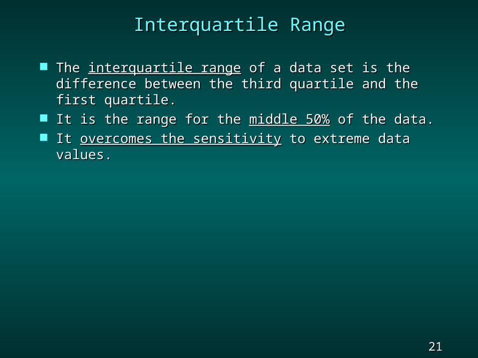
Interquartile RangeInterquartile Range
The The interquartile rangeinterquartile range of a data set is the of a data set is the difference between the third quartile and the first difference between the third quartile and the first quartile.quartile.
It is the range for the It is the range for the middle 50%middle 50% of the data. of the data. It It overcomes the sensitivityovercomes the sensitivity to extreme data to extreme data
values.values.
22 22 Slide Slide
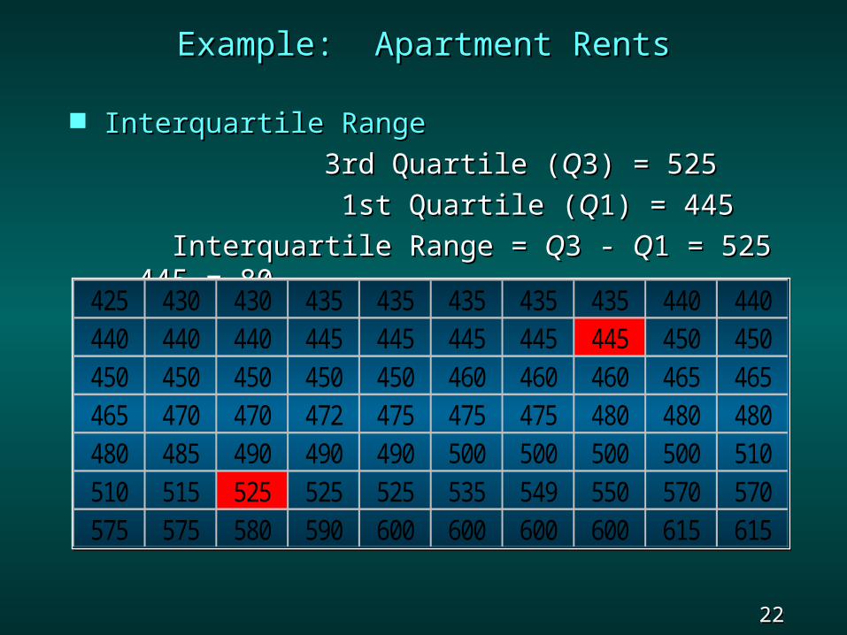
Example: Apartment RentsExample: Apartment Rents
Interquartile RangeInterquartile Range
3rd Quartile (3rd Quartile (QQ3) = 5253) = 525
1st Quartile (1st Quartile (QQ1) = 4451) = 445
Interquartile Range = Interquartile Range = QQ3 - 3 - QQ1 = 525 - 445 = 1 = 525 - 445 = 8080
425 430 430 435 435 435 435 435 440 440440 440 440 445 445 445 445 445 450 450450 450 450 450 450 460 460 460 465 465465 470 470 472 475 475 475 480 480 480480 485 490 490 490 500 500 500 500 510510 515 525 525 525 535 549 550 570 570575 575 580 590 600 600 600 600 615 615
425 430 430 435 435 435 435 435 440 440440 440 440 445 445 445 445 445 450 450450 450 450 450 450 460 460 460 465 465465 470 470 472 475 475 475 480 480 480480 485 490 490 490 500 500 500 500 510510 515 525 525 525 535 549 550 570 570575 575 580 590 600 600 600 600 615 615
23 23 Slide Slide
VarianceVariance
The The variancevariance is a measure of variability that is a measure of variability that utilizes all the data.utilizes all the data.
It is based on the difference between the value It is based on the difference between the value of each observation (of each observation (xxii) and the mean () and the mean (xx for a for a sample, sample, for a population). for a population).
24 24 Slide Slide
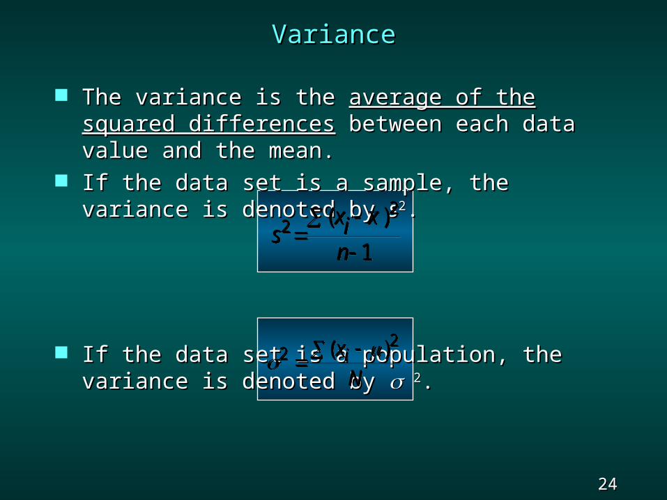
VarianceVariance
The variance is the The variance is the average of the squared average of the squared differencesdifferences between each data value and the between each data value and the mean.mean.
If the data set is a sample, the variance is If the data set is a sample, the variance is denoted by denoted by ss22. .
If the data set is a population, the variance is If the data set is a population, the variance is denoted by denoted by 22..
sxi x
n2
2
1
( )s
xi x
n2
2
1
( )
22
( )xNi 2
2
( )xNi
25 25 Slide Slide
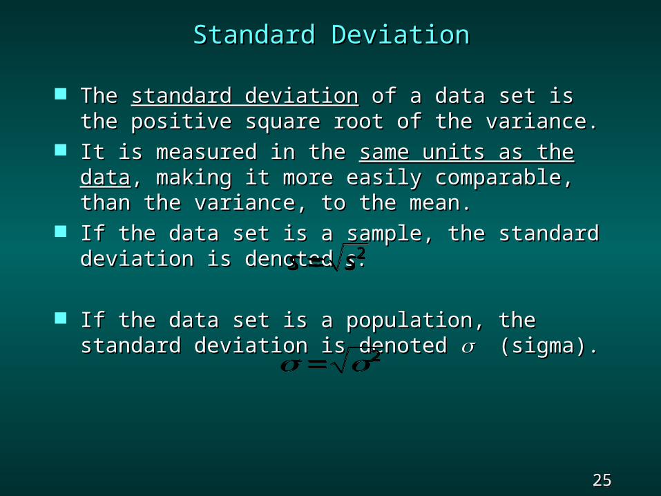
Standard DeviationStandard Deviation
The The standard deviationstandard deviation of a data set is the of a data set is the positive square root of the variance.positive square root of the variance.
It is measured in the It is measured in the same units as the datasame units as the data, , making it more easily comparable, than the making it more easily comparable, than the variance, to the mean.variance, to the mean.
If the data set is a sample, the standard If the data set is a sample, the standard deviation is denoted deviation is denoted ss..
If the data set is a population, the standard If the data set is a population, the standard deviation is denoted deviation is denoted (sigma). (sigma).
s s 2s s 2
2 2
26 26 Slide Slide
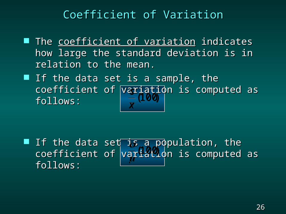
Coefficient of VariationCoefficient of Variation
The The coefficient of variationcoefficient of variation indicates how large indicates how large the standard deviation is in relation to the the standard deviation is in relation to the mean.mean.
If the data set is a sample, the coefficient of If the data set is a sample, the coefficient of variation is computed as follows:variation is computed as follows:
If the data set is a population, the coefficient If the data set is a population, the coefficient of variation is computed as follows:of variation is computed as follows:
sx
( )100sx
( )100
( )100
( )100
27 27 Slide Slide
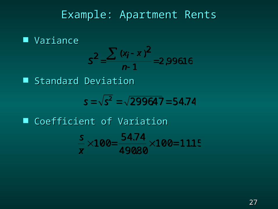
Example: Apartment RentsExample: Apartment Rents
VarianceVariance
Standard DeviationStandard Deviation
Coefficient of VariationCoefficient of Variation
sxi x
n2
2
12 996 16
( ), .s
xi x
n2
2
12 996 16
( ), .
s s 2 2996 47 54 74. .s s 2 2996 47 54 74. .
sx
10054 74490 80
100 11 15..
.sx
10054 74490 80
100 11 15..
.

28 28 Slide Slide
End of Chapter 3, Part AEnd of Chapter 3, Part A
29 29 Slide Slide
Chapter 3 Part B Chapter 3 Part B Descriptive Statistics: Numerical Descriptive Statistics: Numerical
MethodsMethods
Measures of Relative Location and Detecting Measures of Relative Location and Detecting OutliersOutliers
Exploratory Data AnalysisExploratory Data Analysis Measures of Association Between Two Measures of Association Between Two
VariablesVariables The Weighted Mean and The Weighted Mean and
Working with Grouped DataWorking with Grouped Data
%%xx
30 30 Slide Slide
Measures of Relative LocationMeasures of Relative Locationand Detecting Outliersand Detecting Outliers
z-Scoresz-Scores Chebyshev’s TheoremChebyshev’s Theorem Empirical RuleEmpirical Rule Detecting OutliersDetecting Outliers
31 31 Slide Slide
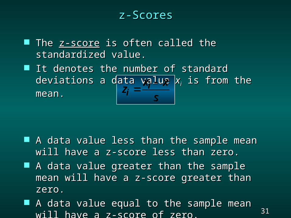
z-Scoresz-Scores
The The z-scorez-score is often called the standardized is often called the standardized value.value.
It denotes the number of standard deviations a It denotes the number of standard deviations a data value data value xxii is from the mean. is from the mean.
A data value less than the sample mean will A data value less than the sample mean will have a z-score less than zero.have a z-score less than zero.
A data value greater than the sample mean A data value greater than the sample mean will have a z-score greater than zero.will have a z-score greater than zero.
A data value equal to the sample mean will A data value equal to the sample mean will have a z-score of zero.have a z-score of zero.
zx xsii
zx xsii
32 32 Slide Slide
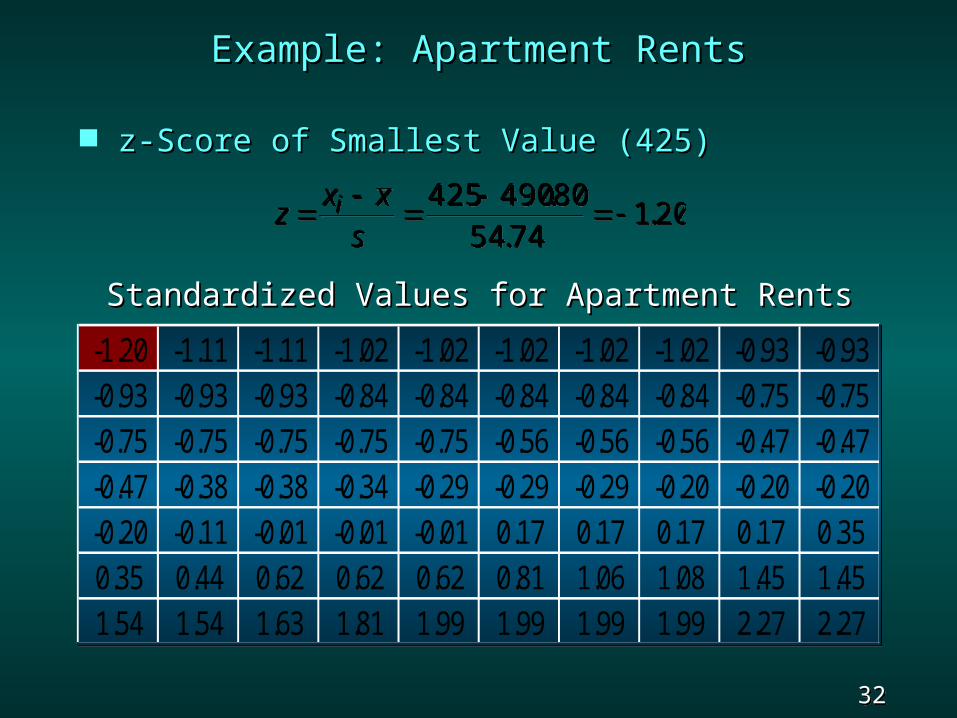
z-Score of Smallest Value (425)z-Score of Smallest Value (425)
Standardized Values for Apartment RentsStandardized Values for Apartment Rents
zx xsi
425 490 80
54 741 20
..
.zx xsi
425 490 80
54 741 20
..
.
-1.20 -1.11 -1.11 -1.02 -1.02 -1.02 -1.02 -1.02 -0.93 -0.93-0.93 -0.93 -0.93 -0.84 -0.84 -0.84 -0.84 -0.84 -0.75 -0.75-0.75 -0.75 -0.75 -0.75 -0.75 -0.56 -0.56 -0.56 -0.47 -0.47-0.47 -0.38 -0.38 -0.34 -0.29 -0.29 -0.29 -0.20 -0.20 -0.20-0.20 -0.11 -0.01 -0.01 -0.01 0.17 0.17 0.17 0.17 0.350.35 0.44 0.62 0.62 0.62 0.81 1.06 1.08 1.45 1.451.54 1.54 1.63 1.81 1.99 1.99 1.99 1.99 2.27 2.27
-1.20 -1.11 -1.11 -1.02 -1.02 -1.02 -1.02 -1.02 -0.93 -0.93-0.93 -0.93 -0.93 -0.84 -0.84 -0.84 -0.84 -0.84 -0.75 -0.75-0.75 -0.75 -0.75 -0.75 -0.75 -0.56 -0.56 -0.56 -0.47 -0.47-0.47 -0.38 -0.38 -0.34 -0.29 -0.29 -0.29 -0.20 -0.20 -0.20-0.20 -0.11 -0.01 -0.01 -0.01 0.17 0.17 0.17 0.17 0.350.35 0.44 0.62 0.62 0.62 0.81 1.06 1.08 1.45 1.451.54 1.54 1.63 1.81 1.99 1.99 1.99 1.99 2.27 2.27
Example: Apartment RentsExample: Apartment Rents
33 33 Slide Slide
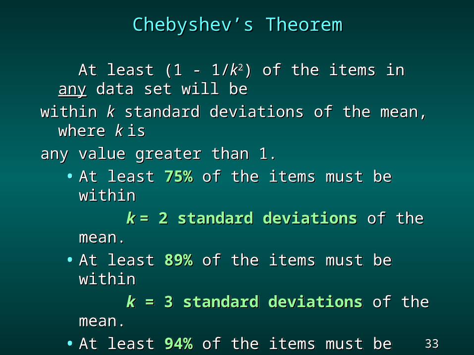
Chebyshev’s TheoremChebyshev’s Theorem
At least (1 - 1/At least (1 - 1/kk22) of the items in ) of the items in anyany data set data set will bewill be
within within kk standard deviations of the mean, where standard deviations of the mean, where k k isis
any value greater than 1.any value greater than 1.
• At least At least 75%75% of the items must be within of the items must be within
k k = 2 standard deviations= 2 standard deviations of the of the mean.mean.
• At least At least 89%89% of the items must be within of the items must be within
kk = 3 standard deviations = 3 standard deviations of the of the mean.mean.
• At least At least 94%94% of the items must be within of the items must be within
kk = 4 standard deviations = 4 standard deviations of the of the mean.mean.
34 34 Slide Slide
Example: Apartment RentsExample: Apartment Rents
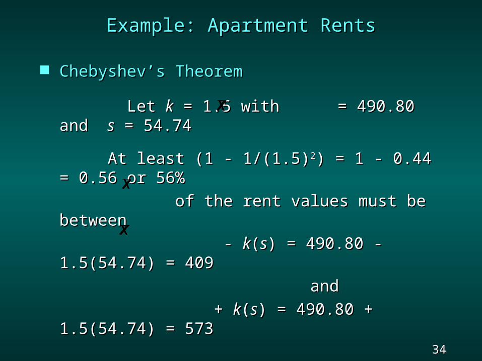
Chebyshev’s TheoremChebyshev’s Theorem
Let Let kk = 1.5 with = 490.80 and = 1.5 with = 490.80 and ss = = 54.7454.74
At least (1 - 1/(1.5)At least (1 - 1/(1.5)22) = 1 - 0.44 = 0.56 or ) = 1 - 0.44 = 0.56 or 56% 56%
of the rent values must be betweenof the rent values must be between
- - kk((ss) = 490.80 - 1.5(54.74) = ) = 490.80 - 1.5(54.74) = 409409
andand
+ + kk((ss) = 490.80 + 1.5(54.74) = ) = 490.80 + 1.5(54.74) = 573573
xx
xx
xx
35 35 Slide Slide
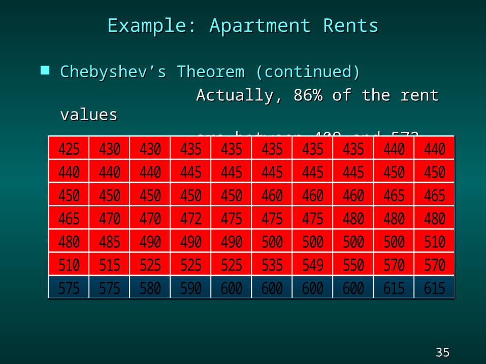
Chebyshev’s Theorem (continued)Chebyshev’s Theorem (continued)
Actually, 86% of the rent valuesActually, 86% of the rent values
are between 409 and 573. are between 409 and 573.
425 430 430 435 435 435 435 435 440 440440 440 440 445 445 445 445 445 450 450450 450 450 450 450 460 460 460 465 465465 470 470 472 475 475 475 480 480 480480 485 490 490 490 500 500 500 500 510510 515 525 525 525 535 549 550 570 570575 575 580 590 600 600 600 600 615 615
425 430 430 435 435 435 435 435 440 440440 440 440 445 445 445 445 445 450 450450 450 450 450 450 460 460 460 465 465465 470 470 472 475 475 475 480 480 480480 485 490 490 490 500 500 500 500 510510 515 525 525 525 535 549 550 570 570575 575 580 590 600 600 600 600 615 615
Example: Apartment RentsExample: Apartment Rents
36 36 Slide Slide
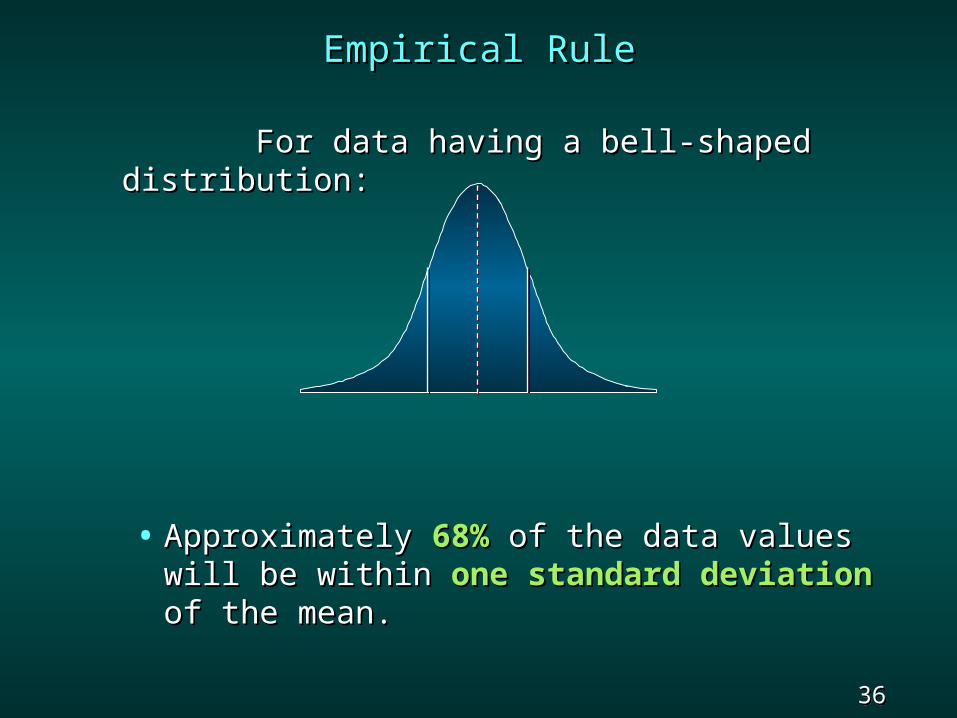
Empirical RuleEmpirical Rule
For data having a bell-shaped distribution:For data having a bell-shaped distribution:
• Approximately Approximately 68%68% of the data values will of the data values will be within be within oneone standard deviationstandard deviation of the of the mean.mean.
37 37 Slide Slide
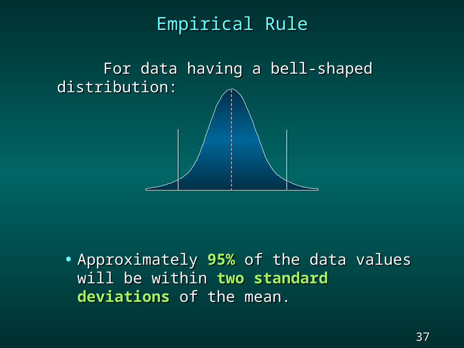
Empirical RuleEmpirical Rule
For data having a bell-shaped For data having a bell-shaped distribution:distribution:
• Approximately Approximately 95%95% of the data values will of the data values will be within be within twotwo standard deviationsstandard deviations of the of the mean.mean.
38 38 Slide Slide
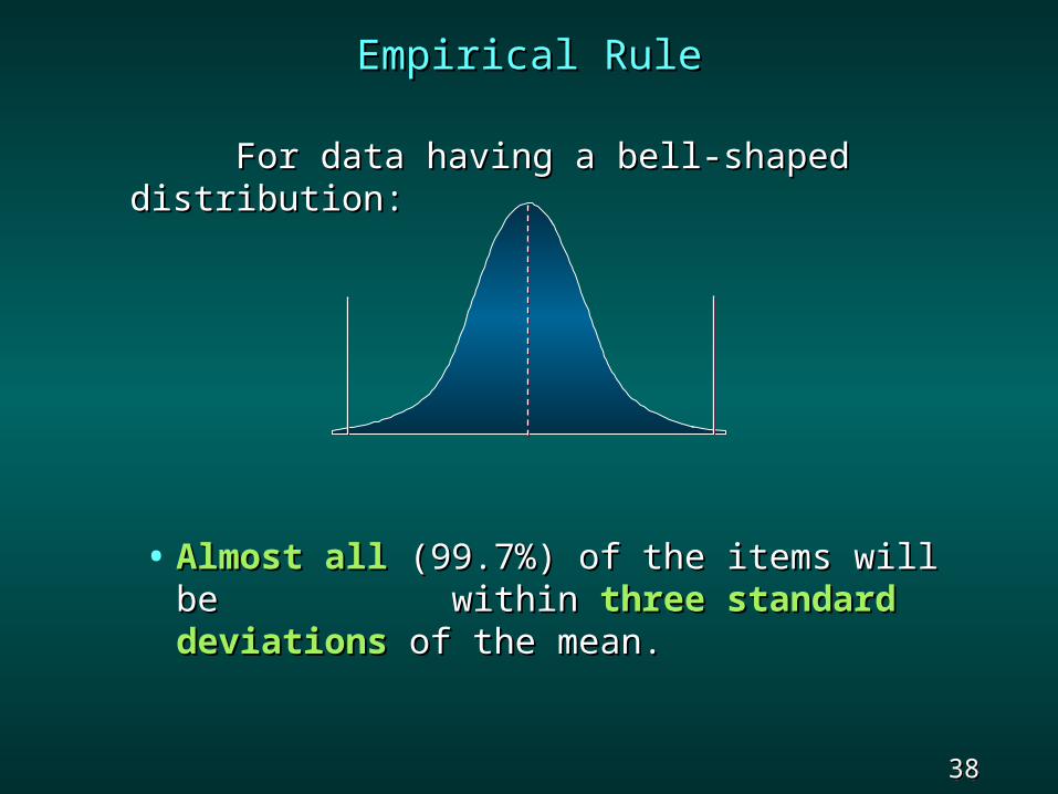
Empirical RuleEmpirical Rule
For data having a bell-shaped For data having a bell-shaped distribution:distribution:
• Almost allAlmost all (99.7%) of the items will be (99.7%) of the items will be within within threethree standard deviationsstandard deviations of the of the mean.mean.
39 39 Slide Slide
Example: Apartment RentsExample: Apartment Rents
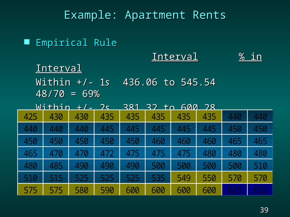
Empirical RuleEmpirical Rule
IntervalInterval % in % in IntervalInterval
Within +/- 1Within +/- 1ss 436.06 to 545.54436.06 to 545.54 48/70 = 48/70 = 69%69%
Within +/- 2Within +/- 2ss 381.32 to 600.28381.32 to 600.28 68/70 = 68/70 = 97%97%
Within +/- 3Within +/- 3ss 326.58 to 655.02326.58 to 655.02 70/70 = 70/70 = 100%100%
425 430 430 435 435 435 435 435 440 440440 440 440 445 445 445 445 445 450 450450 450 450 450 450 460 460 460 465 465465 470 470 472 475 475 475 480 480 480480 485 490 490 490 500 500 500 500 510510 515 525 525 525 535 549 550 570 570575 575 580 590 600 600 600 600 615 615
40 40 Slide Slide
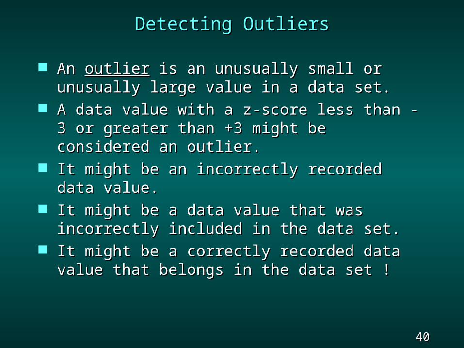
Detecting OutliersDetecting Outliers
An An outlieroutlier is an unusually small or unusually is an unusually small or unusually large value in a data set.large value in a data set.
A data value with a z-score less than -3 or A data value with a z-score less than -3 or greater than +3 might be considered an greater than +3 might be considered an outlier. outlier.
It might be an incorrectly recorded data value.It might be an incorrectly recorded data value. It might be a data value that was incorrectly It might be a data value that was incorrectly
included in the data set.included in the data set. It might be a correctly recorded data value It might be a correctly recorded data value
that belongs in the data set !that belongs in the data set !
41 41 Slide Slide
Example: Apartment RentsExample: Apartment Rents
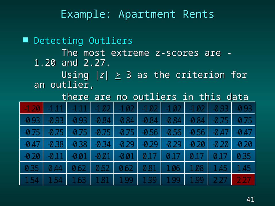
Detecting OutliersDetecting OutliersThe most extreme z-scores are -1.20 and The most extreme z-scores are -1.20 and
2.27.2.27.Using |Using |zz| | >> 3 as the criterion for an 3 as the criterion for an
outlier, outlier, there are no outliers in this data set. there are no outliers in this data set.
Standardized Values for Apartment RentsStandardized Values for Apartment Rents-1.20 -1.11 -1.11 -1.02 -1.02 -1.02 -1.02 -1.02 -0.93 -0.93-0.93 -0.93 -0.93 -0.84 -0.84 -0.84 -0.84 -0.84 -0.75 -0.75-0.75 -0.75 -0.75 -0.75 -0.75 -0.56 -0.56 -0.56 -0.47 -0.47-0.47 -0.38 -0.38 -0.34 -0.29 -0.29 -0.29 -0.20 -0.20 -0.20-0.20 -0.11 -0.01 -0.01 -0.01 0.17 0.17 0.17 0.17 0.350.35 0.44 0.62 0.62 0.62 0.81 1.06 1.08 1.45 1.451.54 1.54 1.63 1.81 1.99 1.99 1.99 1.99 2.27 2.27
-1.20 -1.11 -1.11 -1.02 -1.02 -1.02 -1.02 -1.02 -0.93 -0.93-0.93 -0.93 -0.93 -0.84 -0.84 -0.84 -0.84 -0.84 -0.75 -0.75-0.75 -0.75 -0.75 -0.75 -0.75 -0.56 -0.56 -0.56 -0.47 -0.47-0.47 -0.38 -0.38 -0.34 -0.29 -0.29 -0.29 -0.20 -0.20 -0.20-0.20 -0.11 -0.01 -0.01 -0.01 0.17 0.17 0.17 0.17 0.350.35 0.44 0.62 0.62 0.62 0.81 1.06 1.08 1.45 1.451.54 1.54 1.63 1.81 1.99 1.99 1.99 1.99 2.27 2.27
42 42 Slide Slide
Exploratory Data AnalysisExploratory Data Analysis
Five-Number SummaryFive-Number Summary Box PlotBox Plot
43 43 Slide Slide
Five-Number SummaryFive-Number Summary
Smallest ValueSmallest Value First QuartileFirst Quartile MedianMedian Third QuartileThird Quartile Largest ValueLargest Value
44 44 Slide Slide
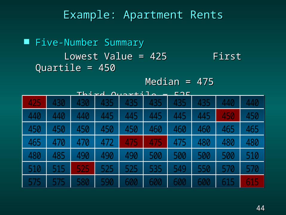
Example: Apartment RentsExample: Apartment Rents
Five-Number SummaryFive-Number Summary
Lowest Value = 425Lowest Value = 425 First Quartile First Quartile = 450= 450
Median = 475Median = 475
Third Quartile = 525 Largest Value Third Quartile = 525 Largest Value = 615= 615425 430 430 435 435 435 435 435 440 440
440 440 440 445 445 445 445 445 450 450450 450 450 450 450 460 460 460 465 465465 470 470 472 475 475 475 480 480 480480 485 490 490 490 500 500 500 500 510510 515 525 525 525 535 549 550 570 570575 575 580 590 600 600 600 600 615 615
425 430 430 435 435 435 435 435 440 440440 440 440 445 445 445 445 445 450 450450 450 450 450 450 460 460 460 465 465465 470 470 472 475 475 475 480 480 480480 485 490 490 490 500 500 500 500 510510 515 525 525 525 535 549 550 570 570575 575 580 590 600 600 600 600 615 615
45 45 Slide Slide
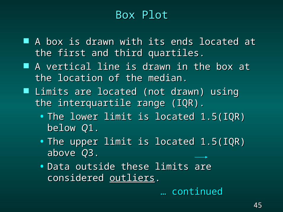
Box PlotBox Plot
A box is drawn with its ends located at the first A box is drawn with its ends located at the first and third quartiles.and third quartiles.
A vertical line is drawn in the box at the A vertical line is drawn in the box at the location of the median.location of the median.
Limits are located (not drawn) using the Limits are located (not drawn) using the interquartile range (IQR).interquartile range (IQR).
• The lower limit is located 1.5(IQR) below The lower limit is located 1.5(IQR) below QQ1.1.
• The upper limit is located 1.5(IQR) above The upper limit is located 1.5(IQR) above QQ3.3.
• Data outside these limits are considered Data outside these limits are considered outliersoutliers..
… … continuedcontinued
46 46 Slide Slide
Box Plot (Continued)Box Plot (Continued)
Whiskers (dashed lines) are drawn from the Whiskers (dashed lines) are drawn from the ends of the box to the smallest and largest ends of the box to the smallest and largest data values inside the limits.data values inside the limits.
The locations of each outlier is shown with the The locations of each outlier is shown with the
symbolsymbol * * ..
47 47 Slide Slide
Example: Apartment RentsExample: Apartment Rents
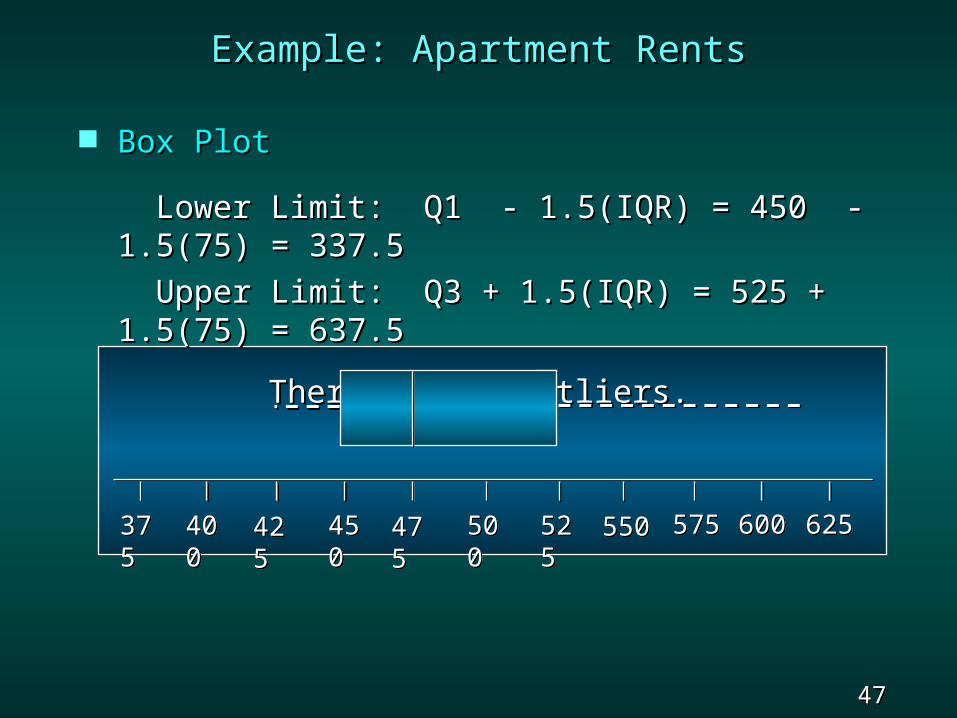
Box PlotBox Plot
Lower Limit: Q1 - 1.5(IQR) = 450 - 1.5(75) Lower Limit: Q1 - 1.5(IQR) = 450 - 1.5(75) = 337.5 = 337.5
Upper Limit: Q3 + 1.5(IQR) = 525 + 1.5(75) Upper Limit: Q3 + 1.5(IQR) = 525 + 1.5(75) = 637.5= 637.5
There are no outliers.There are no outliers.
375375
400400
425425
450450
475475
500500
525525
550550 575575 600600 625625
48 48 Slide Slide
Measures of Association Measures of Association Between Two VariablesBetween Two Variables
CovarianceCovariance Correlation CoefficientCorrelation Coefficient
49 49 Slide Slide
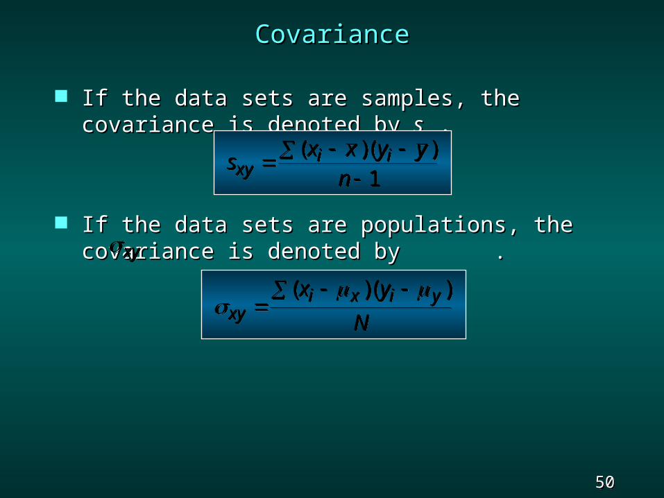
CovarianceCovariance
The The covariancecovariance is a measure of the linear is a measure of the linear association between two variables.association between two variables.
Positive values indicate a positive relationship.Positive values indicate a positive relationship. Negative values indicate a negative Negative values indicate a negative
relationship.relationship.
50 50 Slide Slide
If the data sets are samples, the covariance is If the data sets are samples, the covariance is denoted by denoted by ssxyxy..
If the data sets are populations, the covariance If the data sets are populations, the covariance is denoted by .is denoted by .
CovarianceCovariance
sx x y ynxy
i i
( )( )
1s
x x y ynxy
i i
( )( )
1
xyi x i yx y
N
( )( )
xy
i x i yx y
N
( )( )
xyxy
51 51 Slide Slide
Correlation CoefficientCorrelation Coefficient
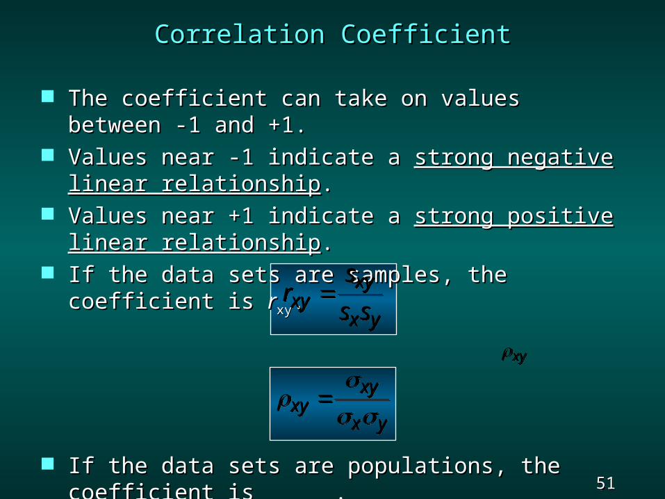
The coefficient can take on values between -1 The coefficient can take on values between -1 and +1.and +1.
Values near -1 indicate a Values near -1 indicate a strong negative linear strong negative linear relationshiprelationship..
Values near +1 indicate a Values near +1 indicate a strong positive linear strong positive linear relationshiprelationship..
If the data sets are samples, the coefficient is If the data sets are samples, the coefficient is rrxyxy..
If the data sets are populations, the coefficient is If the data sets are populations, the coefficient is . .
rs
s sxyxy
x yrs
s sxyxy
x y
xyxy
x y
xyxy
x y
xyxy
52 52 Slide Slide
The Weighted Mean andThe Weighted Mean andWorking with Grouped DataWorking with Grouped Data
Weighted MeanWeighted Mean Mean for Grouped DataMean for Grouped Data Variance for Grouped DataVariance for Grouped Data Standard Deviation for Grouped DataStandard Deviation for Grouped Data
53 53 Slide Slide
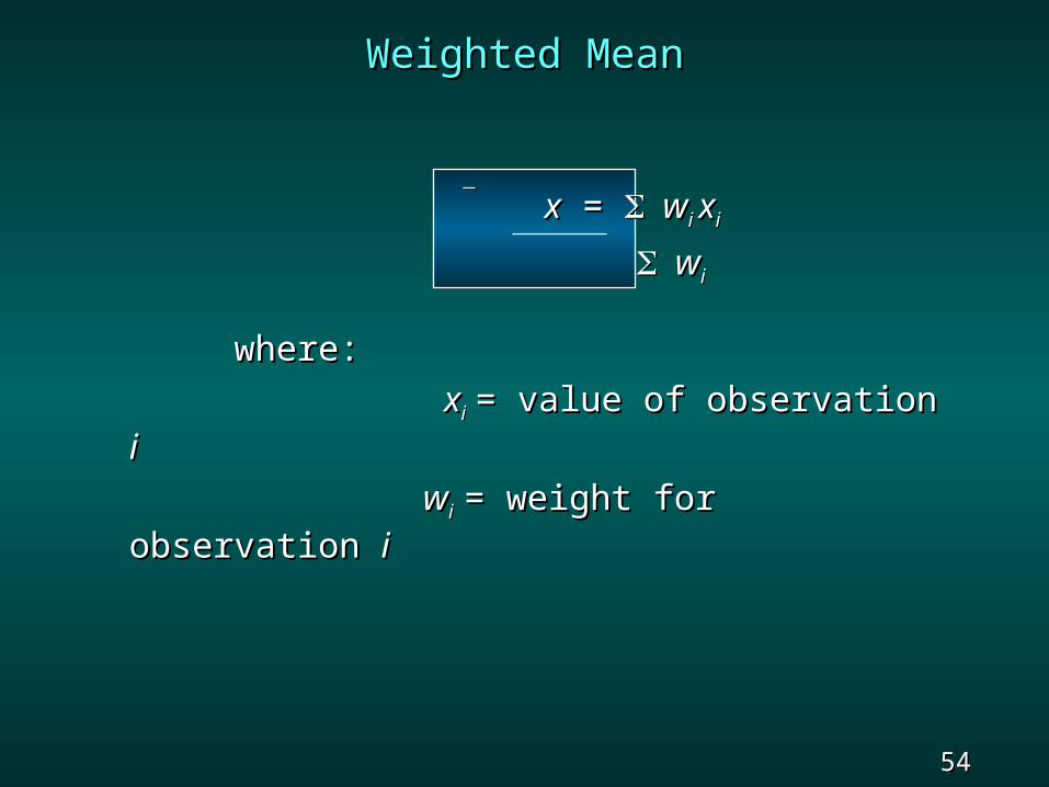
Weighted MeanWeighted Mean
When the mean is computed by giving each When the mean is computed by giving each data value a weight that reflects its data value a weight that reflects its importance, it is referred to as a importance, it is referred to as a weighted weighted meanmean..
In the computation of a grade point average In the computation of a grade point average (GPA), the weights are the number of credit (GPA), the weights are the number of credit hours earned for each grade.hours earned for each grade.
When data values vary in importance, the When data values vary in importance, the analyst must choose the weight that best analyst must choose the weight that best reflects the importance of each value.reflects the importance of each value.
54 54 Slide Slide
Weighted MeanWeighted Mean
xx = = wwi i xxii
wwii
where:where:
xxii = value of observation = value of observation ii
wwi i = weight for observation = weight for observation ii
55 55 Slide Slide
Grouped DataGrouped Data
The weighted mean computation can be used The weighted mean computation can be used to obtain approximations of the mean, to obtain approximations of the mean, variance, and standard deviation for the variance, and standard deviation for the grouped data.grouped data.
To compute the weighted mean, we treat the To compute the weighted mean, we treat the midpoint of each classmidpoint of each class as though it were the as though it were the mean of all items in the class.mean of all items in the class.
We compute a weighted mean of the class We compute a weighted mean of the class midpoints using the midpoints using the class frequenciesclass frequencies as as weights.weights.
Similarly, in computing the variance and Similarly, in computing the variance and standard deviation, the class frequencies are standard deviation, the class frequencies are used as weights.used as weights.
56 56 Slide Slide
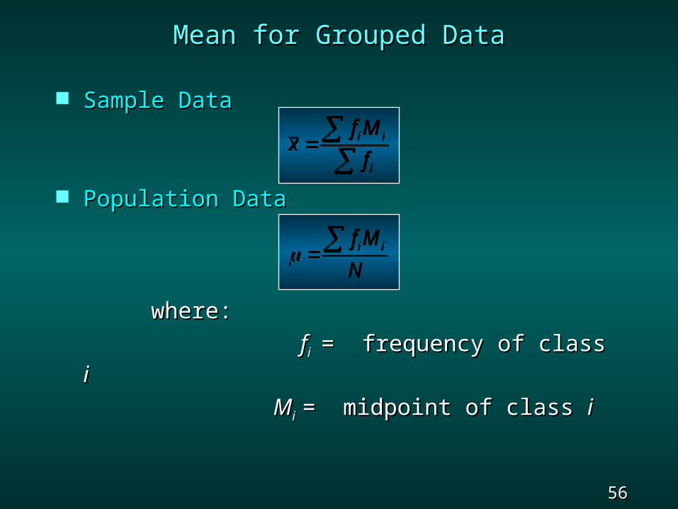
Sample DataSample Data
Population DataPopulation Data
where: where:
ffi i = frequency of class = frequency of class ii
MMi i = midpoint of class = midpoint of class ii
Mean for Grouped DataMean for Grouped Data
i
ii
f
Mfx
i
ii
f
Mfx
N
Mf iiN
Mf ii
57 57 Slide Slide
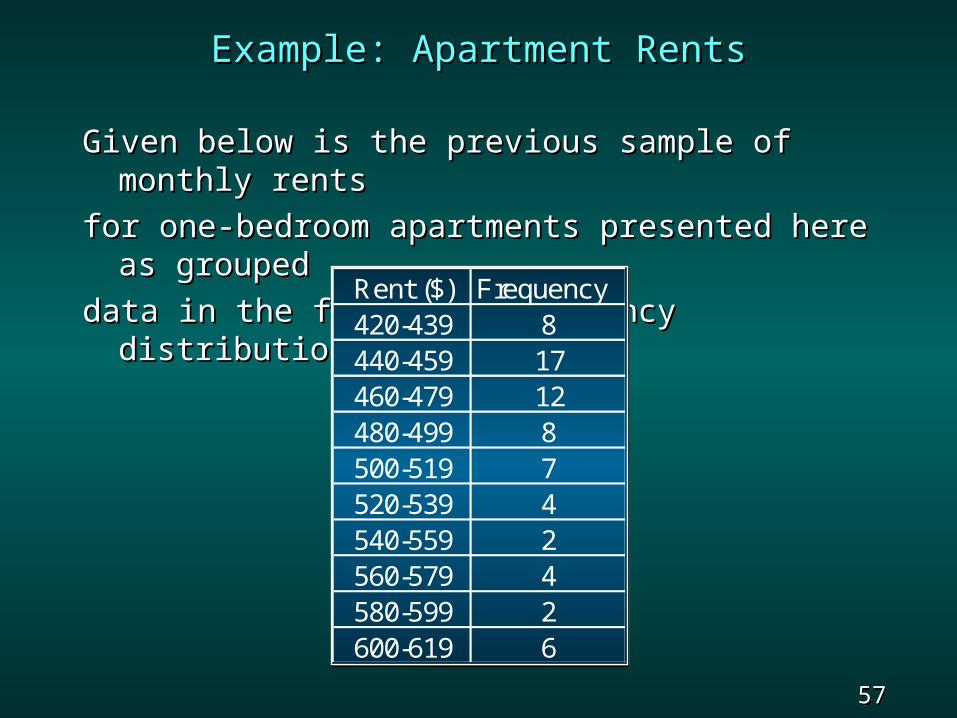
Example: Apartment RentsExample: Apartment Rents
Given below is the previous sample of monthly Given below is the previous sample of monthly rentsrents
for one-bedroom apartments presented here as for one-bedroom apartments presented here as groupedgrouped
data in the form of a frequency distribution. data in the form of a frequency distribution.
Rent ($) Frequency420-439 8440-459 17460-479 12480-499 8500-519 7520-539 4540-559 2560-579 4580-599 2600-619 6
Rent ($) Frequency420-439 8440-459 17460-479 12480-499 8500-519 7520-539 4540-559 2560-579 4580-599 2600-619 6
58 58 Slide Slide
Example: Apartment RentsExample: Apartment Rents
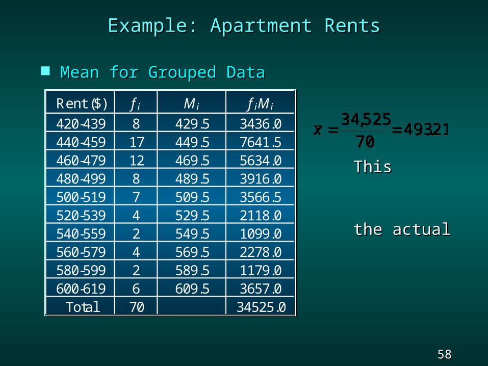
Mean for Grouped DataMean for Grouped Data
This This approximationapproximation differs by $2.41 fromdiffers by $2.41 from
the actual the actual samplesample mean of $490.80.mean of $490.80.
Rent ($) f i M i f iM i
420-439 8 429.5 3436.0440-459 17 449.5 7641.5460-479 12 469.5 5634.0480-499 8 489.5 3916.0500-519 7 509.5 3566.5520-539 4 529.5 2118.0540-559 2 549.5 1099.0560-579 4 569.5 2278.0580-599 2 589.5 1179.0600-619 6 609.5 3657.0
Total 70 34525.0
Rent ($) f i M i f iM i
420-439 8 429.5 3436.0440-459 17 449.5 7641.5460-479 12 469.5 5634.0480-499 8 489.5 3916.0500-519 7 509.5 3566.5520-539 4 529.5 2118.0540-559 2 549.5 1099.0560-579 4 569.5 2278.0580-599 2 589.5 1179.0600-619 6 609.5 3657.0
Total 70 34525.0
x 34 525
70493 21
,.x
34 52570
493 21,
.
59 59 Slide Slide
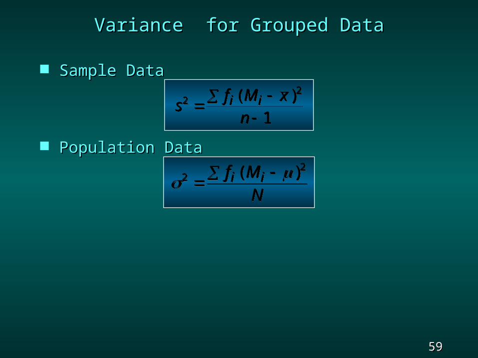
Variance for Grouped DataVariance for Grouped Data
Sample DataSample Data
Population DataPopulation Data
sf M xn
i i22
1
( )s
f M xn
i i22
1
( )
22
f M
Ni i( ) 2
2
f M
Ni i( )
60 60 Slide Slide
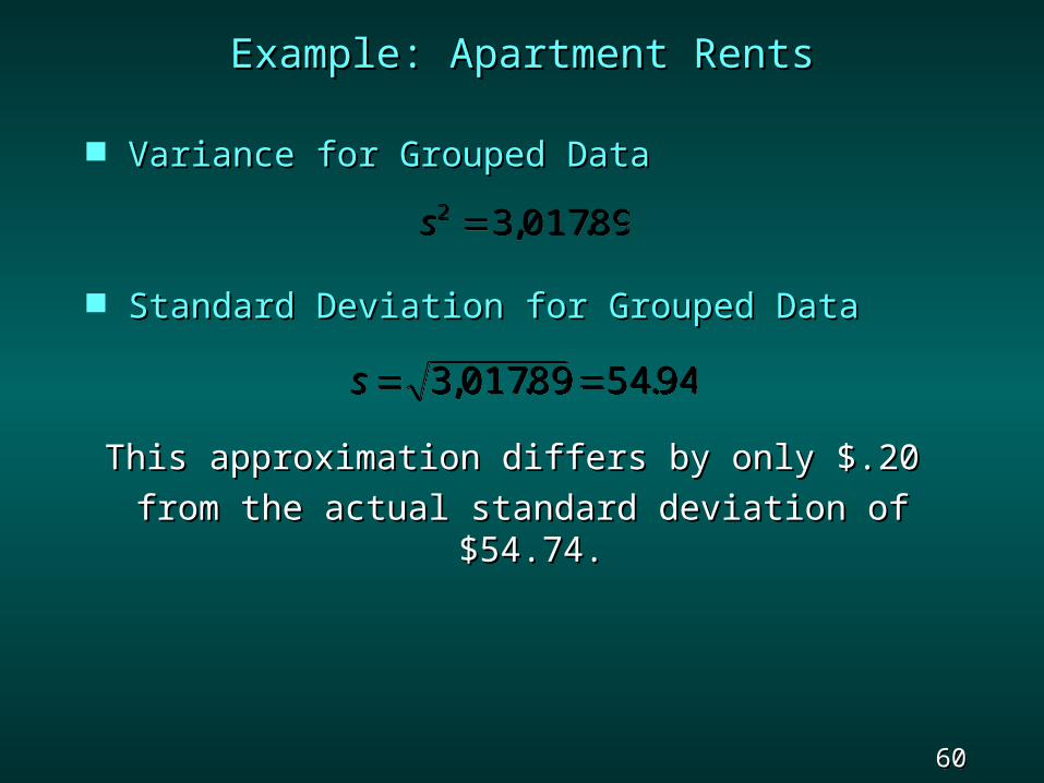
Example: Apartment RentsExample: Apartment Rents
Variance for Grouped DataVariance for Grouped Data
Standard Deviation for Grouped DataStandard Deviation for Grouped Data
This approximation differs by only $.20 This approximation differs by only $.20
from the actual standard deviation of $54.74. from the actual standard deviation of $54.74.
s2 3 017 89 , .s2 3 017 89 , .
s 3 017 89 54 94, . .s 3 017 89 54 94, . .

61 61 Slide Slide
End of Chapter 3, Part BEnd of Chapter 3, Part B