Embed Size (px)
Citation preview
第二讲MIMO系统的模型及容量
Key Laboratory of Antennas and Microwave Technology, Xidian University,China
赵鲁豫, 博士,副教授,博士生导师
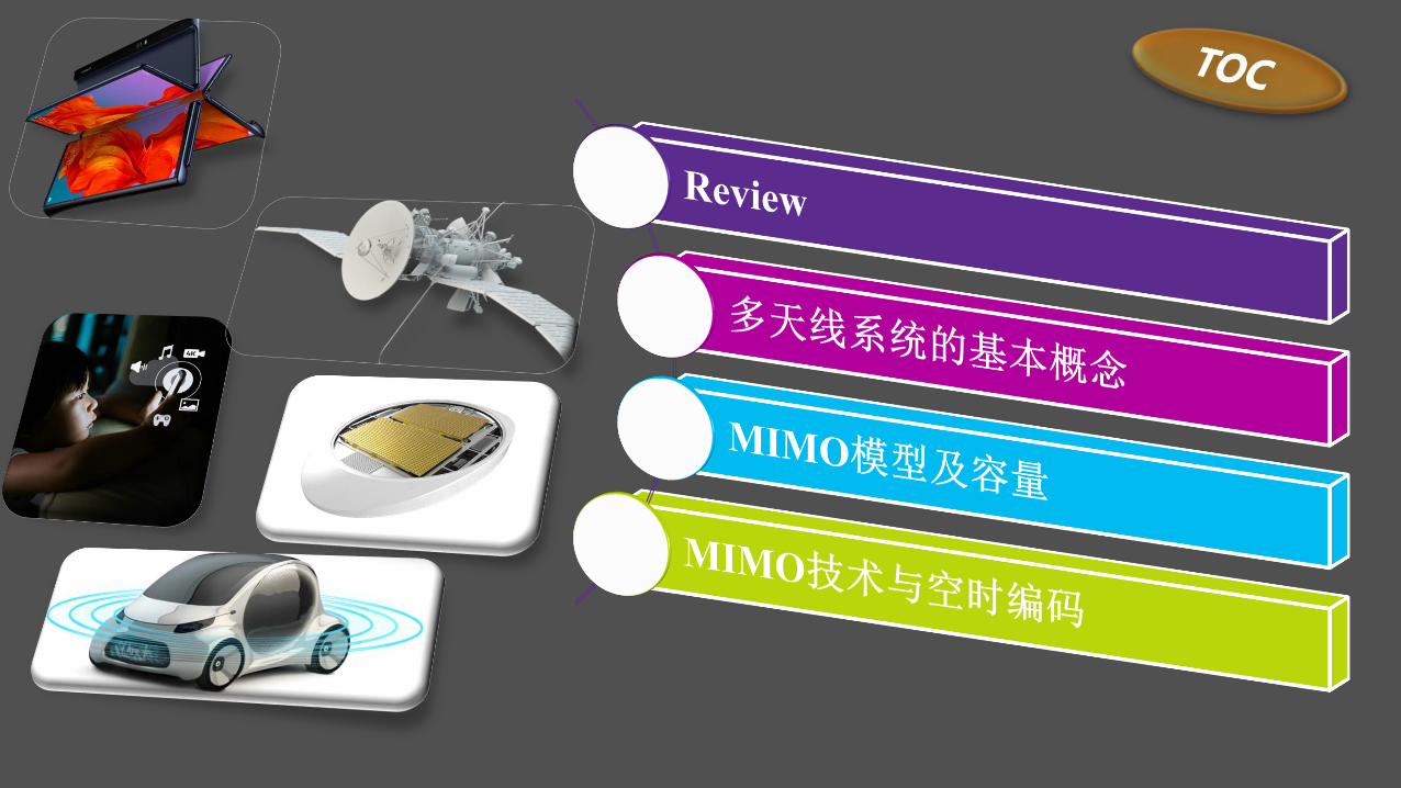

Review1
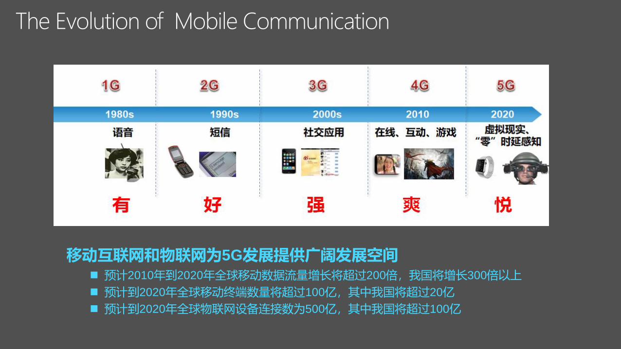
移动互联网和物联网为5G发展提供广阔发展空间◼ 预计2010年到2020年全球移动数据流量增长将超过200倍,我国将增长300倍以上
◼ 预计到2020年全球移动终端数量将超过100亿,其中我国将超过20亿
◼ 预计到2020年全球物联网设备连接数为500亿,其中我国将超过100亿
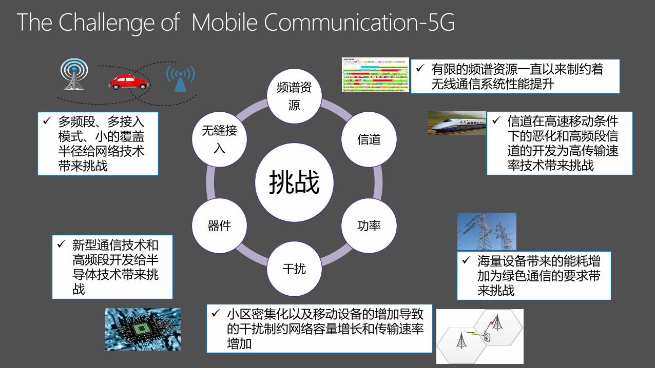
✓ 多频段、多接入模式、小的覆盖半径给网络技术带来挑战
✓ 新型通信技术和高频段开发给半导体技术带来挑战
✓ 海量设备带来的能耗增加为绿色通信的要求带来挑战
✓ 信道在高速移动条件下的恶化和高频段信道的开发为高传输速率技术带来挑战
✓ 有限的频谱资源一直以来制约着无线通信系统性能提升
✓ 小区密集化以及移动设备的增加导致的干扰制约网络容量增长和传输速率增加
挑战
频谱资
源
信道
功率
干扰
器件
无缝接
入

多天线系统的基本概念2
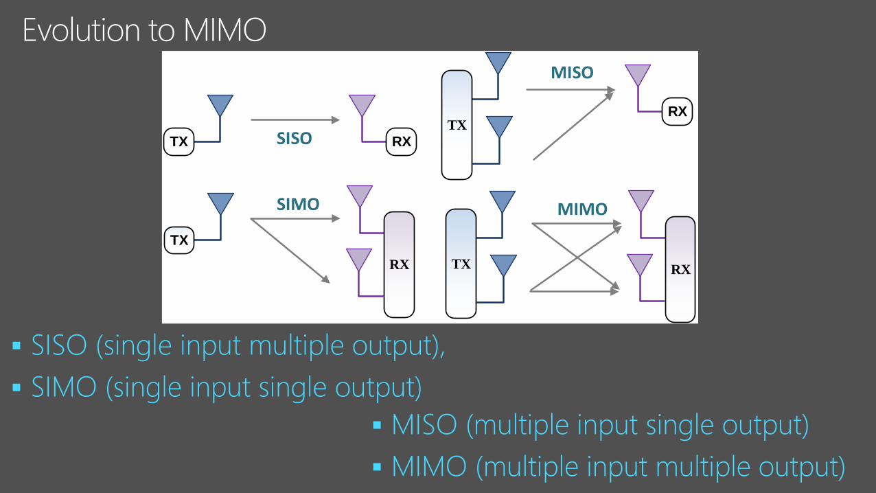
▪
▪
TX RXSISO
TX
SIMO
RX
RX
MISO
TX
MIMO
RXTX
▪
▪
▪
▪
▪
▪
▪
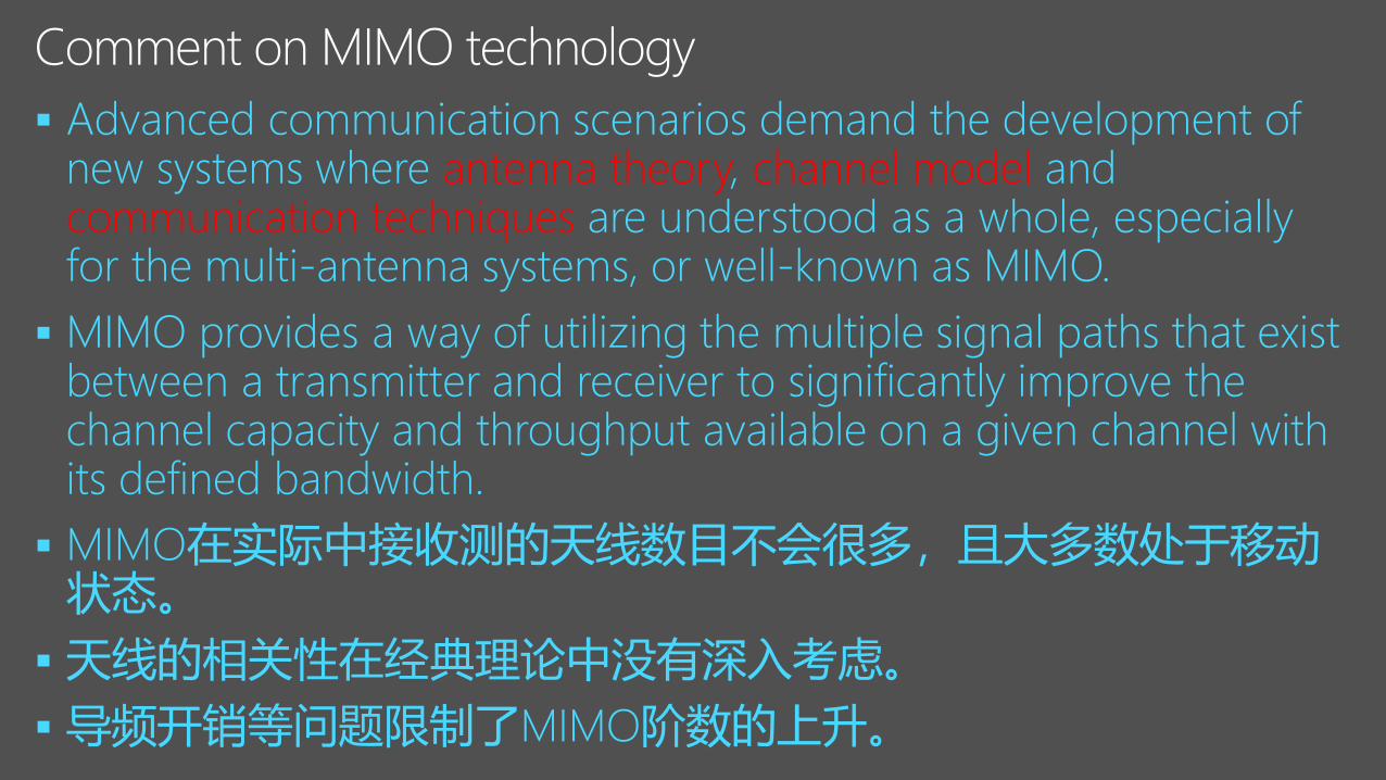
antenna theory channel modelcommunication techniques
▪
▪
▪
▪

MIMO的模型及容量3

▪
𝒚 =𝐸𝑠𝑁𝐇𝒔 + 𝒏
𝒚 is a M× 1 vector representing received signal
𝒔 is a 𝑁 × 1 transmitted signal vector
𝒏 is an additive noise vector
𝐇 is a M× N channel matrix
(a single user MIMO over a fading channel with AWGN)
Additive White Gaussian Noise
𝐸𝑠 is the total energy at the Tx within a symbol period
(2.1)
𝐑𝒚𝒚 =𝐸𝑠𝑁𝐇𝐑𝐬𝐬𝐇
𝐻 +𝑁0𝐈𝑀
▪
(2.2)
N0 is the noise power
where 𝐑𝐬𝐬 = ℰ 𝒔𝒔𝐻 is the covariance of 𝐬, N0 is the noise power.
▪
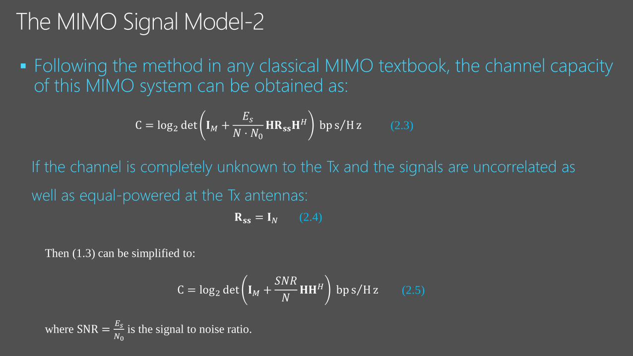
C = log2 det 𝐈𝑀 +𝐸𝑠
𝑁 ⋅ 𝑁0𝐇𝐑𝐬𝐬𝐇
𝐻 bp Τs H z (2.3)
If the channel is completely unknown to the Tx and the signals are uncorrelated as
well as equal-powered at the Tx antennas:
𝐑𝐬𝐬 = 𝐈𝑁 (2.4)
C = log2 det 𝐈𝑀 +𝑆𝑁𝑅
𝑁𝐇𝐇𝐻 bp Τs H z (2.5)
where SNR =𝐸𝑠
𝑁0is the signal to noise ratio.
Then (1.3) can be simplified to:

▪ never
• The antennas at both Tx and Rx
are always correlated because of
limited antenna spacing
• The antennas at both Tx and Rx are
always correlated because of
imperfect pattern orthogonality
• The antennas at both Tx and Rx are
always correlated because of poor port
isolation
LTE/3G Baseband
BT/WiFi Baseband
LTE/3G RF BT/WiFi RF
ANT1 ANT3
Interference from ISM band
Interference from LTE/3G
GPS
Baseband
GPS RF
ANT2
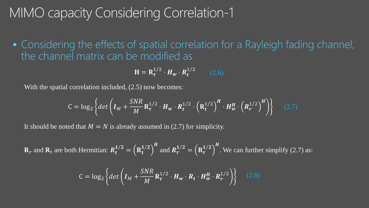
▪
𝐇 = 𝐑𝐫Τ1 2 ⋅ 𝑯𝒘 ⋅ 𝑹𝒕
Τ1 2(2.6)
With the spatial correlation included, (2.5) now becomes:
C = log2 𝑑𝑒𝑡 𝑰𝑀 +𝑆𝑁𝑅
𝑀𝐑𝐫
Τ1 2 ⋅ 𝑯𝒘 ⋅ 𝑹𝒕Τ1 2 ⋅ 𝐑𝐭
Τ1 2𝑯⋅ 𝑯𝒘
𝑯 ⋅ 𝑹𝒓Τ1 2
𝑯(2.7)
It should be noted that 𝑀 = 𝑁 is already assumed in (2.7) for simplicity.
𝐑r and 𝐑t are both Hermitian: 𝑹𝒕Τ𝟏 𝟐 = 𝐑𝐭
Τ𝟏 𝟐𝑯
and 𝑹𝒓Τ𝟏 𝟐 = 𝐑𝐫
Τ𝟏 𝟐𝑯
. We can further simplify (2.7) as:
C = log2 𝑑𝑒𝑡 𝑰𝑀 +𝑆𝑁𝑅
𝑀𝐑𝐫
Τ1 2 ⋅ 𝑯𝒘 ⋅ 𝑹𝒕 ⋅ 𝑯𝒘𝑯 ⋅ 𝑹𝒓
Τ1 2 (2.8)

Under high SNR condition: 𝑆𝑁𝑅 ≫ 1, (2.8) becomes:
C = log2 𝑑𝑒𝑡𝑆𝑁𝑅
𝑀𝐑𝐫
Τ1 2 ⋅ 𝑯𝒘 ⋅ 𝑹𝒕 ⋅ 𝑯𝒘𝑯 ⋅ 𝑹𝒓
Τ1 2(2.9)
Using the property that det 𝐀 ⋅ 𝐁 = det 𝐀 ⋅ det 𝐁 = det 𝐁 ⋅ 𝐀 , (2.9) yields:
C ≈ log2 𝑑𝑒𝑡𝑆𝑁𝑅
𝑁𝑯𝒘𝑯𝒘
𝑯 + log2 𝑑𝑒𝑡 𝑹𝑟 + log2 𝑑𝑒𝑡 𝑹𝑡 (2.10)
It can be proved that log2 𝑑𝑒𝑡 𝑹𝑟 ≤ 0 and log2 𝑑𝑒𝑡 𝑹𝑡 ≤ 0 [R1],
Therefore, the higher the correlation, the smaller the channel capacity.
[R1] A. Paulraj, R. Nabar, and D. Gore, Introduction to Space-Time Wireless Communications. Cambridge, U.K.: Cambridge Univ. Press, 2003, pp77.
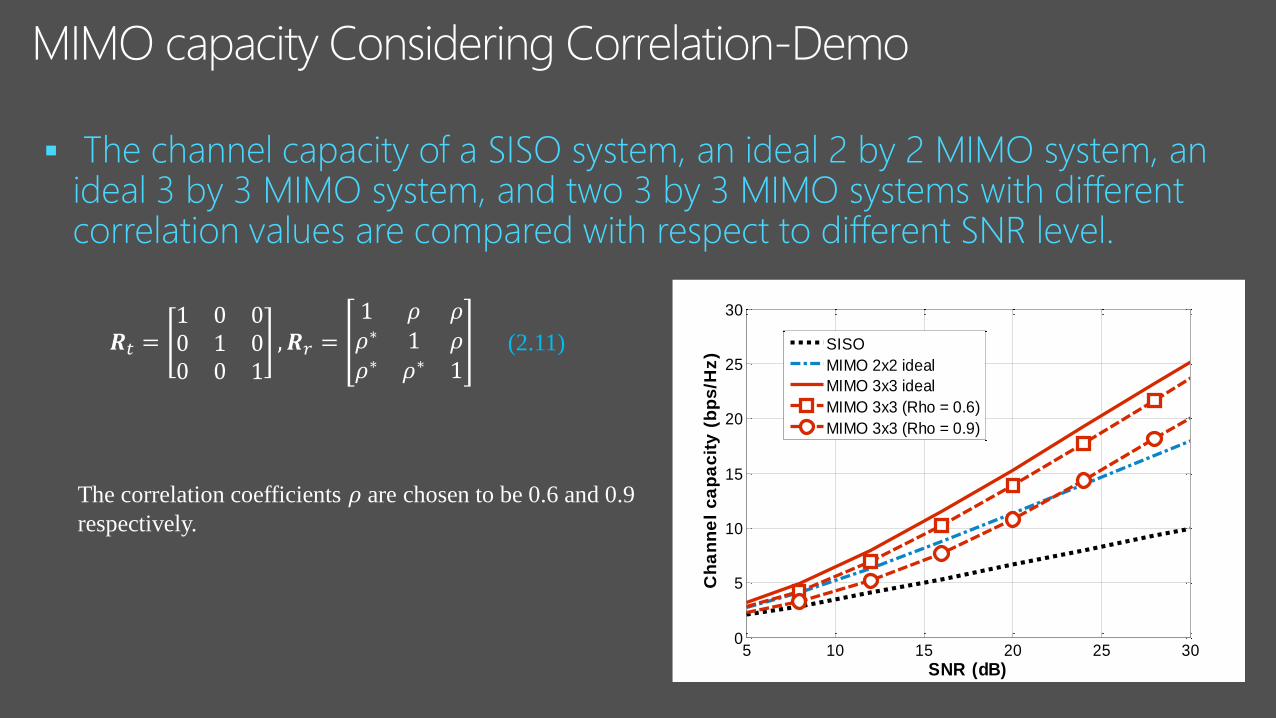
▪
5 10 15 20 25 300
5
10
15
20
25
30
SNR (dB)
Ch
an
ne
l c
ap
ac
ity
(b
ps
/Hz
)
SISO
MIMO 2x2 ideal
MIMO 3x3 ideal
MIMO 3x3 (Rho = 0.6)
MIMO 3x3 (Rho = 0.9)
𝑹𝑡 =1 0 00 1 00 0 1
, 𝑹𝑟 =
1 𝜌 𝜌𝜌∗ 1 𝜌𝜌∗ 𝜌∗ 1
(2.11)
The correlation coefficients 𝜌 are chosen to be 0.6 and 0.9
respectively.

▪
• 要求1: 可以改变阶数,如2x2, 3x3。• 要求2:相关系数可以从0到1之间任意变化。• 要求3:结果可视化,可以画出曲线。• 挑战要求:实现基于MATLAB的GUI
• 思考1:此时考虑的相关系数,和天线计算得到的ECC有什么关系?• 思考2:相关系数选择多少作为评判相关性低的标准合适?• 思考3:𝑀 ≠ 𝑁的时候,Channel Capacity怎么计算
MIMO技术与SpaceTime Coding4
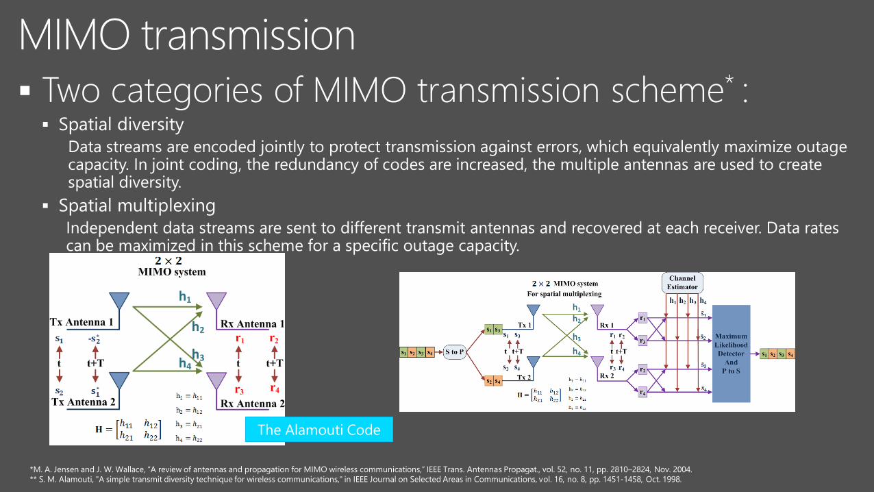
▪
▪
▪
*M. A. Jensen and J. W. Wallace, “A review of antennas and propagation for MIMO wireless communications,” IEEE Trans. Antennas Propagat., vol. 52, no. 11, pp. 2810–2824, Nov. 2004.
** S. M. Alamouti, "A simple transmit diversity technique for wireless communications," in IEEE Journal on Selected Areas in Communications, vol. 16, no. 8, pp. 1451-1458, Oct. 1998.
The Alamouti Code

▪
This paper is selected as one of
the 57 best papers over 50 years!
*S. M. Alamouti, "A simple transmit diversity technique for wireless communications," in IEEE Journal on Selected Areas in Communications, vol. 16, no. 8, pp. 1451-1458, Oct. 1998.

▪
▪
▪
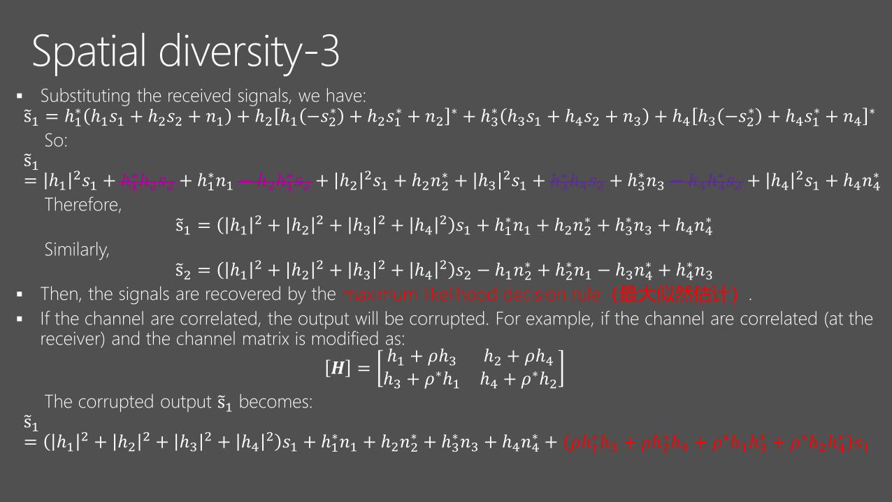
▪
ℎ1∗ℎ2𝑠2 − ℎ2ℎ1
∗𝑠2 ℎ3∗ℎ4𝑠2 − ℎ4ℎ3
∗𝑠2
▪ maximum likelihood decision rule(最大似然估计)
▪
𝜌ℎ1∗ℎ3 + 𝜌ℎ2
∗ℎ4 + 𝜌∗ℎ1ℎ3∗ + 𝜌∗ℎ2ℎ4
∗ 𝑠1
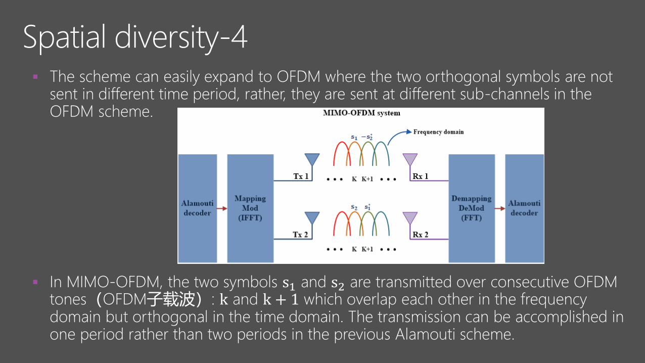
▪ The scheme can easily expand to OFDM where the two orthogonal symbols are not sent in different time period, rather, they are sent at different sub-channels in the OFDM scheme.
▪ In MIMO-OFDM, the two symbols s1 and s2 are transmitted over consecutive OFDM tones(OFDM子载波): k and k + 1 which overlap each other in the frequency domain but orthogonal in the time domain. The transmission can be accomplished in one period rather than two periods in the previous Alamouti scheme.