04122006

8/8/2019 04122006

http://slidepdf.com/reader/full/04122006 1/40

Pride and Prejudice:

The Human Side of Incentive Theory

Tore Ellingsen∗ Magnus Johannesson∗∗

November 29, 2006(Under revision)

Abstract

Many people are sensitive to social esteem, and their pride is a sourceof pro–social behavior. We present a game-theoretic model in whichsensitivity to esteem varies across players and may depend on contextas well players’ beliefs about their opponents. For example, the prideassociated with a generous image is greater when the player holding theimage is in fact generous and believes the observers to be generous as

well. The model can account both for the fact that players’ behaviorsometimes depends on the opponents’ unchosen options and for theprevalence of small symbolic gifts. Perhaps most importantly, the modeloffers an explanation for motivational crowding out: Control systemsand pecuniary incentives may erode morale by signaling to the agentthat the principal is not worth impressing.

JEL classification: D01, D23, D82, Z13

Keywords: Motivational crowding out, Esteem, Incentives, Framing,Social preferences.

∗Address: Department of Economics, Stockholm School of Economics, Box 6501, S—11383 Stockholm, Sweden. Email: [email protected].

∗∗Address: Department of Economics, Stockholm School of Economics, Box 6501, S—11383 Stockholm, Sweden. Email: [email protected].

We are grateful to the Torsten and Ragnar Soderberg Foundation (Ellingsen) and theSwedish Research Council (Johannesson) for financial support. Thanks to George Baker,Kjell-Arne Brekke, Florian Englmaier, Ernst Fehr, Martin Floden, Oliver Hart, Bengt Holm-strom, John Moore, Anna Sjogren, Jean-Robert Tyran, Robert Ostling, and especiallyMichael Kosfeld for helpful discussions. The paper has also benefited from comments bymany other seminar and conference participants. Errors are ours.

1

8/8/2019 04122006


1 Introduction

Nature, when she formed man for society, endowed himwith an original desire to please, and an original aversionto offend his brethren. She taught him to feel pleasure intheir favourable, and pain in their unfavourable regard.She rendered their approbation most flattering and mostagreeable to him for its own sake; and their disapproba-tion most mortifying and most offensive.

Adam Smith (1790, Part III, Section I, Paragraph 13)

Few controversies in the social sciences are more heated than the debate

over incentive theory. For example, in the field of organizational behavior,microeconomic incentive theory is frequently regarded as outright dangerous.McGregor’s (1960) celebrated management book The Human Side of Enter-prise argued that managers who subscribe to the conventional view that em-ployees dislike work – McGregor labelled it Theory X – may create workerswho are “resistant, antagonistic, uncooperative” (page 38). That is, manage-rial control and material incentives may trigger the very behaviors that theyare designed to avert. Conversely, managers who subscribe to the more opti-mistic view that employees see their work as a source of self-realization andsocial esteem – Theory Y – may create workers who voluntarily seek to fulfill

the organization’s goals.1

Any theory of incentives must be based on assumptions about human na-ture, and the theorist must balance the desire for realism against the desirefor parsimony. Over the last decade, microeconomists working on incentivetheory have become increasingly inclined to discard the common simplifica-tion – the cornerstone of Theory X – that people are guided solely by materialself–interest.2 To a considerable extent, the change in attitude is due to empir-ical studies that document the prediction failures of Theory X. Two prominentobservations are the wage level puzzle that higher wages sometimes induce bet-ter performance (Fehr, Kirchsteiger and Riedl, 1993, Bewley, 1999), and theincentive intensity puzzle that stronger monetary incentives sometimes induceworse performance (Frey and Oberholzer-Gee, 1997, Gneezy and Rusticini,

1For an updated version of the arguments against Theory X, see Chapter 4 of Pfeffer(1994), aptly entitled “Wrong Heroes, Wrong Theories, and Wrong Language.”

2Kreps (1997) and Baron and Kreps (1999) are watershed contributions. Others arementioned below. In a recent survey that seems representative of the current mainstreamview, Sobel (2005, page 432) concludes that the assumption of narrow selfishness shouldnot be taken for granted: “A philosophical refusal to consider extended preferences leads toawkward explanations of some phenomena. It limits the questions that can be asked andrestricts the answers. It is a handicap.”

2

8/8/2019 04122006


2000a, 2000b, Bohnet, Frey and Huck, 2001, Fehr and Gachter, 2002, Fehr

and Rockenbach, 2003, and Fehr and List, 2004). Both observations violate thestandard principal–agent model, which predicts that the agent’s effort shouldbe unaffected by the level of pay, and that stronger incentives should always en-tail higher effort.3 The incentive intensity puzzle aptly illustrates McGregor’scritique: A principal who believes that agents are opportunistic has reason toutilize relatively strong material incentives, and when these incentives createmore opportunistic behavior, the principal’s belief is self-fulfilling.

While theories of fairness and reciprocity can account for the wage levelpuzzle, they generally fail to explain the incentive intensity puzzle. Thus,theorists have recently turned to other explanations, closer to the territory of

McGregor’s Theory Y. In two recent papers, Benabou and Tirole have arguedthat private information could be the culprit. The first paper, Benabou and Ti-role (2003), focuses on self-realization and shows that material incentives mightbackfire if offered by a principal who is more knowledgeable than the agent,because the agent may interpret the incentive as bad news about his talent orabout the difficulty of the task. Benabou and Tirole (2006) instead focuses onsocial esteem and shows that material incentives might likewise backfire whenthe agent has private information about multiple personal characteristics, suchas materialism and altruism (see Seabright, 2004, for a related argument). Forexample, an altruistic agent may donate less blood after the introduction of an incentive, because the incentive will be attractive to materialistic types andhence dilute the signaling value of blood donation.4 Although Benabou andTirole’s two models have considerable explanatory power, they both fail toexplain a striking regularity uncovered in recent experimental studies by Fehrand Rockenbach (2003), Fehr and List (2004), and Falk and Kosfeld (2005),namely that material incentives have a negative effect on agents’ performanceeven when the principal lacks private information about the agent’s character-istics, but only when (the agent knows that) the principal can choose whetheror not to impose the incentive. Thus, the question is: Why does the principal’schoice set matter even though the principal lacks private information aboutthe agent?

In this paper, we propose a model that can explain why the principal’schoice set matters even when the principal lacks information about the agent’stype. According to our model, the principal’s distrust has a negative effect on

3We here abstract from the effect of wealth changes on labor supply. In most of theempirical studies, wealth effects can safely be assumed to be negligible due to low stakesand short horizons.

4Titmuss (1970) famously originated the idea that material incentives crowd out volun-tary blood donation. For a supportive field experiment, see Mellstrom and Johannesson(2006).

3

8/8/2019 04122006


agents’ effort because low expectations are demoralizing. The argument builds

on two key assumptions. The first assumption is that people care about socialesteem and therefore want to signal favorable traits; in this respect, our modelis closely related to Benabou and Tirole (2006).5 The second assumption isthat the value of esteem depends on the audience. We want to be thought wellof by all people, but it also matters who thinks well of us. Roughly put, theagent wants the principal’s respect, but more so if the principal is respectable.6

We think that both our assumptions are uncontroversial. While most peo-ple certainly do seek material rewards, immaterial rewards like esteem or socialstatus matter too. Thus, a person may work hard not only to earn a largermaterial reward and to contribute to society, but also in order to make a fa-

vorable impression. Chester Barnard (1938, page 145) put it succinctly: “Theopportunities for distinction, prestige, personal power, and the attainment of dominating positions are much more important than material rewards in thedevelopment of all sorts of organizations, including commercial organizations.”Psychologists from Maslow (1943) to Baumeister and Leary (1995) agree thatesteem is a fundamental source of motivation, as did the classical thinkers,from the Greeks to Adam Smith; see Brennan and Pettit (2004, Chapter 1).In fact, it seems to us that almost everyone realizes that making a good impres-sion is rewarded through the respect, attention, and tribute paid by principals,peers, or other observers. Likewise, it is widely agreed that the value of re-spect depends on its source. As David Hume (1739, Book II, Part I, Sect. XI)expresses it in his account of humans’ fundamental love of fame: “tho famein general be agreeable, yet we receive a much greater satisfaction from theapprobation of those, whom we ourselves esteem and approve of, than those,whom we hate and despise.” Hume’s student, Adam Smith (1790, Part II, Sec-tion III, Paragraph 10), articulates the same idea: “What most of all charmsus in our benefactor, is the concord between his sentiments and our own, withregard to what interests us so nearly as the worth of our own character, andthe esteem that is due to us.”

At a general level, our model offers a new approach to the modelling of reciprocity. In the reciprocity literature, a major question has been to explain

the important role that people appearently ascribe to others’ intentions. Two

5Although human concern for social esteem has been well understood for a long time, thefirst satisfactory formal model of signalling for esteem purposes is probably due to Bernheim(1994).

6This is not to say that ruthless principals can exploit their agents by pretending to berespectable: In equilibrium, respectable principals can only convey their respectability byengaging in costly signalling. That is, in order to credibly signal their faith in Theory Y theprincipal must be either more optimistic or more concerned with social esteem than are theprincipals who subscribe to Theory X.

4

8/8/2019 04122006


previous explanations have been formalized. Levine (1998) suggests that peo-

ple’s altruism or spite depend on their beliefs about their opponents, and thatthis may explain reciprocity. For example, if a player is more altruistic towardother altruists, a generous action by an opponent may be rewarded, and a lessgenerous action may be punished - because it is a signal that altruism is low. If the situation is the same, except the opponent does not have the opportunityto be generous, lack of altruism can no longer be inferred, and the same actionmay go unpunished. Our model is closely related to Levine’s inasmuch as wetoo focus on signaling and the impact of the opponents’ type on a players’utility. However, in Levine’s model players do not mind what opponents thinkabout them, as long as it does not affect their behavior. One argument in favor

of our approach over Levine’s is that we can potentially explain why behaviorin experiments like the Dictator game does not always end up at corners of the feasible set when stakes are small.7 According to Levine’s model, eitheraltruism, spite, or selfishness ought to be the dominant motive in this case -so subjects ought to give all or nothing. (If fairminded subjects are allowed,there might also be a spike at the equal split.) When people seek social esteem,behavior may be interior as players engage in exactly the amount of altruismor spitefulness that is necessary to signal their type to others. Giving, say,twenty percent of one’s endowment in the Dictator game then makes sense asa strategy to stand out from the group of selfish and spiteful subjects.

A second way to accommodate intention–based reciprocity is to allow agentsto have preferences defined directly over others’ actions, not only over out-comes. This approach, which builds on concepts introduced by Geanakopolos,Pearce, and Stacchetti (1989), has been pioneered by Rabin (1993), Charnessand Rabin (2002), Dufwenberg and Kirchsteiger (2005), and Falk and Fis-chbacher (2006). While this model is fascinating and potentially useful forunderstanding reciprocity, it is rather complicated and it takes a longer stepaway from conventional game theoretic models than we do. More importantly,it fails to explain the incentive intensity puzzle identified by Falk and Kosfeld(2005).

Before presenting our model, let us therefore fix ideas by considering Falk

and Kosfeld’s experimental evidence on the hidden costs of control. Their set-ting is maximally simple. An agent has an endowment of 120 money units andcan make transfers to the principal. For every unit that the agent gives up,the principal receives two units. Hence, the principal can receive an amount of at least 0 and at most 240. Before the agent decides how much to transfer vol-untarily, the principal has the opportunity to impose a compulsory transfer of

7Rotemberg (2006) discusses some other shortcomings of Levine’s model and proposes asolution to them.

5

8/8/2019 04122006


10 (receiving 20). Note that all conventional theories, and even the intention–

based reciprocity model of Falk and Fischbacher (2006), predict that the prin-cipal should control the agent. The reason is that only a relatively selfish agentwould ever give less than 10, and if the agent is selfish trusting her makes nosense. In stark contrast, Falk and Kosfeld find that the majority of principalstrust their agent, abstaining from the compulsory transfer, and also that suchtrust on average pays significantly better than distrust. One achievement of our model is to rationalize Falk and Kosfeld’s findings.8

2 A model of pride and prejudice

There are already many models in which players are assumed to care aboutthe beliefs of others, i.e., to be proud. Our model will add the seemingly minortwist that not everyone is equally proud, and that not every opponent’s belief is equally important.

In addition to differential pride, we will admit heterogeneous beliefs. Thisassumption, which generates a role for prejudice, is less common. Althoughmost of our qualitative results can be derived with heterogeneous pride alone,we argue that heterogeneous beliefs could be quantitatively important for un-derstanding much of the experimental evidence.

2.1 Players and actions

There are two players.9 We restrict attentions to games in which each playermoves at most once. The set of (pure) actions for player i is denoted Ai and ageneric action is denoted ai. Mixed actions are probability distributions overAi. Let X denote the set of mixed actions.

8Sliwka (2003) and Ellingsen and Johannesson (2005) have explored the closely relatedidea that incentives may backfire by conveying pessimistic expectations, thereby reducingagents’ feeling of guilt in case of shirking. (The first paper uses psychological game theory;the second, like us, uses a conventional signaling model.) In other words, material incen-

tives backfire because pessimistic expectations legitimize opportunism; a similar mechanismis hinted at in Charness and Dufwenberg, 2005. If this explanation were correct, the lessopportunistic agents would feel relieved whenever the principal imposed non-binding con-straints on them. Falk and Kosfeld (2005) document that agents are frustrated – not relieved– when subjected to control, whether it is binding or not.

9The analysis is straightforwardly extended to the case of more players, but at somenotational cost.

6

8/8/2019 04122006


2.2 Characteristics

Players are heterogeneous. A player’s type is given by a vector of characteris-tics, or personality traits, θi ∈ Θ = (Θ1,..., Θn) ⊂ R

n+.

Each agent’s type is drawn independently from the same joint distributionf t(θ), with the associated joint cumulative distribution function F t(θ). (At thecost of cluttering the notation, we could instead let the two agents’ types bedrawn from separate distributions.)

2.3 Beliefs

In order to accommodate the heterogeneity in beliefs that is observed in expri-

ments, we assume that players beliefs about the opponent’s type are correlatedwith their own types. Instead of just assuming the correlation, we provideprimitive assumptions that generate it.10 To this end, we assume that the truedistribution is not known to the agents; they only know that the distributionis drawn from a set of joint cumulative distribution functions F .

The set F is common knowledge between the players. We also assume thatthe distribution from which F t is drawn is common knowledge. However, sinceplayers know their own types, and these types may differ, Bayesian updatingimplies that players may hold different beliefs about each other. We say thatthe players have a common metaprior , but that they have different – and

privately known – priors.Let p0i = p(F |θi) denote player i’s prior on the joint distribution (the prob-

ability density over the set of possible cumulative distributions), and let p0kidenote the associated prior about the marginal distribution of trait k. In otherwords, p0i is player i’s initial beliefs about player j. As the game progresses,players will update their beliefs. Let hi denote the history of actions observedby player i when it is i’s turn to move, and let pi(θ j|hi, θi) denote i’s conditionalbelief about j’s type. Finally, let ˆ p j denote i’s belief about (the function) p j.

If the game is sequential, we assume that players update their beliefs usingBayes’ rule following any action by the opponent.

10It is well known that people tend to think that others are like them. Psychologistsinitially concluded that people therefore systematically overestimate the degree of similarity– creating a “false–consensus” effect; see Ross, Green and House (1977). However, as notedby Dawes (1989), it is rational to use information about one’s own inclinations to infer thelikely inclinations of others. Our model will capture the rational consensus effect alluded toby Dawes. (We take no stand on the issue of whether empirically observed consensus effectsare primarily rational or not.)

7

8/8/2019 04122006


2.4 Strategies and solution concepts

The model centers around the effect that an agent’s action ai has on the oppo-nent’s posterior belief, and especially how actions are affected by the strategicmotive to influence these beliefs. The solution concept is perfect Bayesian equi-librium (PBE) and refinements thereof. Since we confine attention to games inwhich each player moves at most once, the set of possible histories for playeri when moving is Hi = {A j ∪ ∅}.

A strategy for player i is a mapping σi : Θ×F×Hi → X . In words, player i’s(mixed) action depends on the own type, the belief about the opponent’s type,and any observed prior actions by the opponent. We seek pairs of strategies(σ∗

1, σ∗2) and beliefs ( p∗1, p∗2) such that σ∗

i is a best response to σ∗ j given the

beliefs p∗i and we require that p∗1 and p∗2 satisfy Bayes’ rule whenever it applies.In addition, we insist that the beliefs are “reasonable” off the equilibrium pathin the sense that they satisfy either the Never a Weak Best Response (NWBR)property of Cho and Kreps (1987) or the (stronger) D1 criterion of Cho andSobel (1990); for formal definitions and comparisons of these solution concepts,see for example Fudenberg and Tirole (1991).11 Finally, we insist that beliefsabout the opponent’s conditional beliefs are correct on the equilibrium path,i.e., (ˆ p1, ˆ p2) = ( p∗1, p∗2). The latter assumption is probably the strongest of allour assumptions; to us it is not even clear that players should hold correctbeliefs about the opponent’s prior after learning the opponent’s type.

2.5 Preferences

Players care both about the material consequences of their actions and aboutwhat the opponent will think about them.12 More precisely, they care aboutthe opponent’s assessment of their type.

For simplicity, we assume that players only care about first moments. Let

rk j = E [θki |θ j, h j]

denote player j’s assessment, or rating , of player i’s characteristic k. The rating

potentially depends both on player j’s type – since the type affects the priorbelief – and on any move that i has taken.

The key elements of the model concern the impact of others’ rating onplayers’ utility. We allow player i’s sensitivity to player j’s rating to depend on

11As usual in signaling games, the main results would survive, subject to suitable restric-tions on the players’ priors, if we instead were to apply the Undefeated Equilibrium conceptof Mailath, Okuno-Fujiwara and Postlewaite (1993).

12In principle, players may also care about what other spectators think. We return to thisissue below.

8

8/8/2019 04122006


what i thinks about j’s personality. For example, appreciation for skilfulness is

sweeter when it comes from others who are skilled. On the other hand, revengeis sweet primarily when observed by the perpetrator. Thus, we probably wantour gifts to be observed by altruists and our punishments to be observed byegoists. The impact of others’ beliefs on a player’s utility is also allowed todepend on which traits are salient in the situation. Some situations call forgenerosity, others for courage, and the distinction between situations can besubtle. For example, in an otherwise identical situation, the personality traitsthat are salient for someone dressed as a soldier may be less so for someonedressed as a vicar.

To capture the dependence of players utility on opponents’ characteristics

and the nature of the situation, let sij = (s1

ij,...,sn

ij) : Θ × Θ →Rn

+ be theweights that player i’s assign to player j’s rating; we refer to sij as player i’ssalience weights. In the applications that we consider in this paper, we shallmake the simplification that salience weights are independent of i’s own type.Thus, we shall let s j = s(θ j) be the weight that player i puts on the assessmentof player j of type θ j.

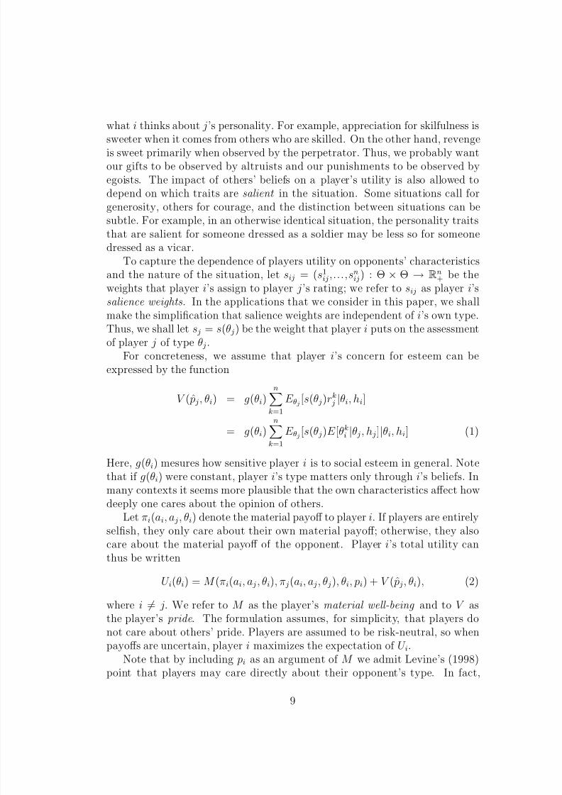
For concreteness, we assume that player i’s concern for esteem can beexpressed by the function

V (ˆ p j, θi) = g(θi)n

k=1

E θj [s(θ j)rk j |θi, hi]

= g(θi)n

k=1

E θj [s(θ j)E [θki |θ j, h j]|θi, hi] (1)

Here, g(θi) mesures how sensitive player i is to social esteem in general. Notethat if g(θi) were constant, player i’s type matters only through i’s beliefs. Inmany contexts it seems more plausible that the own characteristics affect howdeeply one cares about the opinion of others.

Let πi(ai, a j, θi) denote the material payoff to player i. If players are entirelyselfish, they only care about their own material payoff; otherwise, they alsocare about the material payoff of the opponent. Player i’s total utility can

thus be written

U i(θi) = M (πi(ai, a j , θi), π j(ai, a j, θ j), θi, pi) + V (ˆ p j, θi), (2)

where i = j. We refer to M as the player’s material well-being and to V asthe player’s pride. The formulation assumes, for simplicity, that players donot care about others’ pride. Players are assumed to be risk-neutral, so whenpayoffs are uncertain, player i maximizes the expectation of U i.

Note that by including pi as an argument of M we admit Levine’s (1998)point that players may care directly about their opponent’s type. In fact,

9

8/8/2019 04122006


our model nests both Levine (1998) and Benabou and Tirole (2006) as special

cases. Compared to Levine’s model, the main innovation is the function V .Compared to Benabou and Tirole’s model, the main innovation is the symmet-ric treatment of the two players; in their setting, only one player cares aboutpride, and only one player holds private information. In order to focus sharplyon our contribution, we shall henceforth dispense with the key ingredients of both Levine and of Benabou and Tirole: We assume that M is independent of pi and, for most of the time, that players’ characteristics are uni-dimensional.

2.6 The two-type case

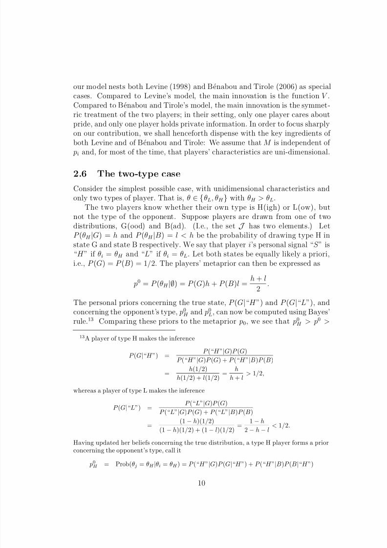
Consider the simplest possible case, with unidimensional characteristics andonly two types of player. That is, θ ∈ {θL, θH } with θH > θL.The two players know whether their own type is H(igh) or L(ow), but

not the type of the opponent. Suppose players are drawn from one of twodistributions, G(ood) and B(ad). (I.e., the set J has two elements.) LetP (θH |G) = h and P (θH |B) = l < h be the probability of drawing type H instate G and state B respectively. We say that player i’s personal signal “S ” is“H ” if θi = θH and “L” if θi = θL. Let both states be equally likely a priori,i.e., P (G) = P (B) = 1/2. The players’ metaprior can then be expressed as

p0 = P (θH

|∅) = P (G)h + P (B)l =h + l

2.

The personal priors concerning the true state, P (G|“H ”) and P (G|“L”), andconcerning the opponent’s type, p0H and p0L, can now be computed using Bayes’rule.13 Comparing these priors to the metaprior p0, we see that p0H > p0 >

13A player of type H makes the inference

P (G|“H ”) =P (“H ”|G)P (G)

P (“H ”|G)P (G) + P (“H ”|B)P (B)

=h(1/2)

h(1/2) + l(1/2)=

h

h + l> 1/2,

whereas a player of type L makes the inference

P (G|“L”) =P (“L”|G)P (G)

P (“L”|G)P (G) + P (“L”|B)P (B)

=(1 − h)(1/2)

(1 − h)(1/2) + (1 − l)(1/2)=

1 − h

2 − h − l< 1/2.

Having updated her beliefs concerning the true distribution, a type H player forms a priorconcerning the opponent’s type, call it

p0H = Prob(θj = θH |θi = θH ) = P (“H ”|G)P (G|“H ”) + P (“H ”|B)P (B|“H ”)

10

8/8/2019 04122006


p0L. Despite starting out with a common view of the world, type H is more

optimistic about the opponent than is type L.In the two–type case, pi(θi) denotes player i’s conditional belief that θ j =

θH , and ˆ p j(θ j) denotes player i’s belief that player j believes that θi = θH . LetsI be the weight that player i assigns to the assessment of player j of type I,where I ∈ {L, H }. Then, the level of pride for player i of type I is

V i(ˆ p j, θI ) = g(sI )[ pi(θI )sH [ˆ p j(θH )θH + (1 − ˆ p j(θH ))θL]

+(1 − pi(θI ))sL[ˆ p j(θL)θH + (1 − ˆ p j(θL))θL]]. (3)

Note how player i likes to impress player j; i’s pride is increasing in ˆ p j . Im-

portantly, j’s type matters to player i’s pride. If sH > sL, it is more valuablefor player i to impress player j the more likely it is that player j is of typeH. As we shall see, this may create an additional incentive, over and above j’sown pride, for player j to convey the impression of being type H.

The model is ready for its first test.

3 The trust game

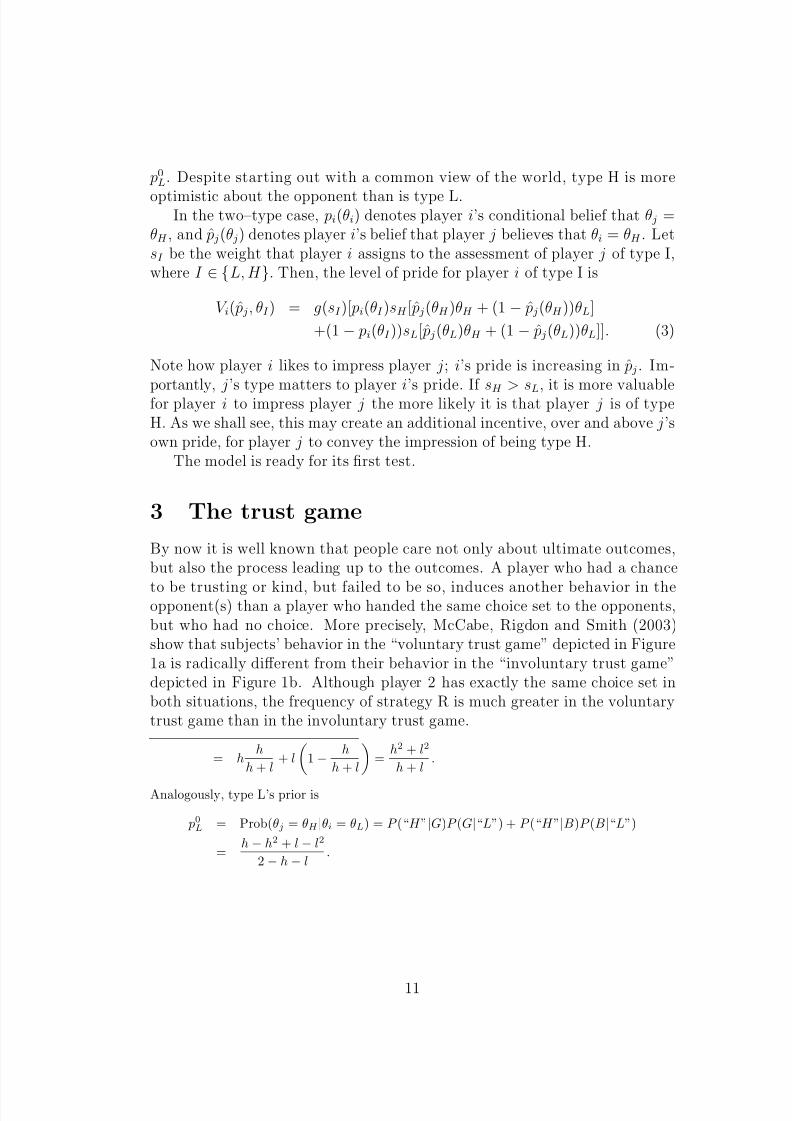
By now it is well known that people care not only about ultimate outcomes,but also the process leading up to the outcomes. A player who had a chance

to be trusting or kind, but failed to be so, induces another behavior in theopponent(s) than a player who handed the same choice set to the opponents,but who had no choice. More precisely, McCabe, Rigdon and Smith (2003)show that subjects’ behavior in the “voluntary trust game” depicted in Figure1a is radically different from their behavior in the “involuntary trust game”depicted in Figure 1b. Although player 2 has exactly the same choice set inboth situations, the frequency of strategy R is much greater in the voluntarytrust game than in the involuntary trust game.

= hh

h + l+ l

1 −

h

h + l

=

h2 + l2

h + l.

Analogously, type L’s prior is

p0L = Prob(θj = θH |θi = θL) = P (“H ”|G)P (G|“L”) + P (“H ”|B)P (B|“L”)

=h − h2 + l − l2

2 − h − l.

11

8/8/2019 04122006


1

2

20, 20

15, 30 25, 25

1

2

15, 30 25, 25

NT

T

N R

Figure 1a: Voluntary trust

T

N R

Figure 1b: Involuntary trust

.....................................................................................................................................

.

.

.

.

.

.

.

.

.............

.

.

.

.

.

.

.

.

.

.

.

.

.

.

.

.

.

.

.

.

.

.

.

.

.

.

.

.

.

.

.

.

.

.

.

.

.

.

.

.

.

.

.

.

.

.

.

.

.

.

.

.

.

.

.

.

.

.

.

.

.

.

.

.

.

.

.

.

.

.

.

.

.

.

.

.

.

.

.

.

.

.

.

.

.

.

.

.

.

.

.

.

.

.

.

.

.

.

.

.

.

.

.

.

.

.

.

.

.

.

.

.

.

.

.

.

.

.

.

.

.

.

.

.

.

.

.

.

.

.

.

.

.

.

.

.

.

.

.

.

.

.

.

.

.

.

.

.

.

.

.

.

.

.

.

.

.

.

.

.

.

.

.

.

.

.

.

.

.

.

.

.

.

.

.

.

.

.

.

.

.

.

.

.

.

.

.

.

.

..

.................................................................................................................................................................................................

..........................................

..

.................................................................................................................................................................................................

..........................................

.

.

.

.

.

.

.

.

.

.............

.

.

.

.

.

.

.

.

.

.

.

.

.

.

.

.

.

.

.

.

.

.

.

.

.

.

.

.

.

.

.

.

.

.

.

.

.

.

.

.

.

.

.

.

.

.

.

.

.

.

.

.

.

.

.

.

.

.

.

.

.

.

.

.

.

.

.

.

.

.

.

.

.

.

.

.

.

.

.

.

.

.

.

.

.

.

.

.

.

.

.

.

.

.

.

.

.

.

.

.

.

.

.

.

.

.

.

.

.

.

.

.

.

.

.

.

.

.

.

.

.

.

.

.

.

.

.

.

.

.

.

.

.

.

.

.

.

.

.

.

.

.

.

.

.

.

.

.

.

.

.

.

.

.

.

.

.

.

.

.

.

.

.

.

.

.

.

.

.

.

.

.

.

.

.

.

.

.

.

.

.

.

.

.

.

.

.

.

.

...................................................................................................................................................................................................

..........................................

..

..

...............................................................................................................................................................................................

..........................................

To see how our model rationalizes this experimental finding, we must firstask what is the source of heterogeneity among players, i.e., what is the salientcharacteristic of a player when in this situation? Since monetary payoffs aregiven exogenously, it must be some social preference. Let us posit that therelevant characteristic is inequality aversion of the kind proposed by Fehr andSchmidt (1999), and that for simplicity the preferences of player i can be

written U i = πi − |πi − π j|θi + V (ˆ p j, θi). (4)

The formulation implies that a player’s “superiority aversion” is as strong asthe player’s “inferiority aversion”; it is straightforward to relax this assump-tion. Another plausible generalization would be to introduce internal salienceweights to account for the fact that even the purely personal aversion to in-equality may depend on the situation.

Let us start by analyzing the problem of player 2 in the involuntary trustgame. We want to derive a condition under which player 2 chooses N (notreward) regardless of his type. Since type H players have most to gain by

playing R (reward), we impose the out–of–equilibrium belief restriction thatplay of R will be interpreted as a sure sign that player 2 is type H. A type Hplayer then chooses to play N if

30 − (30 − 25)θH

+ [ p0H sH ( p0H θH + (1 − p0H )θL) + (1 − p0H )sL( p0LθH + (1 − p0L)θL)]gH

> 25 + [ p0H sH θH + (1 − p0H )sL)θH ]gH ,

12

8/8/2019 04122006


or equivalently

gH <5(1 − θH )

(θH − θL)(1 − p0H )( p0H sH + (1 − p0L)sL). (5)

We see that a necessary condition is θH < 1, which is all right as Fehr andSchmidt usually sets θH = 0.6. The corresponding condition for a type L playeris obviously weaker, so we can neglect it.

Turning to the voluntary trust game, player 2 of type H is supposed to playR. Given the proposed equilibrium expectations, the type H player plays R if

25 + gH θH sH > 30 − θH (30 − 15) + gH θLsH ,

or equivalently

gH >5 − 15θH

(θH − θL)sH

. (6)

Player 2 of type L is supposed to play N and will do so if

25 + gLθH sH < 30 − θL(30 − 15) + gLθLsH ,

or equivalently

gL <5 − 15θL

(θH − θL)sH

. (7)

Finally, player 1 of type H is willing to play T if

p0H (25 + gH θH sH ) + (1 − p0H )(15 − θH (30 − 15) + gH θH sL)

> 20 + p0H gH θLsH + (1 − p0H )gH θLsL,

or equivalently

p0H >5 + 15θH − (θH − θL)gH sL

10 + 20θH + (θH − θL)(sH − sL)gH

, (8)

whereas player 1 of type L is willing to play NT if

p0L(25 + gLθH sH ) + (1 − p0L)(15 + gLθH sL)

< 20 + p0LgLθLsH + (1 − p0L)gLθLsL,

or equivalently

p0L <5 − (θH − θL)gLsL

10 + (θH − θL)(sH − sL)gL. (9)

It is immediate from (5), (6), and (7) that there is an open set of parametervectors (gL, gH , p0L, p0H , sL, sH , θL, θH ) such that all these three conditions hold.

13

8/8/2019 04122006


Moreover, this is true for any priors ( p0L, p0H ). Since we can always find priors

such that both (8) and (9) hold, we have proved that there is an open setof parameters such that type H trusts in the role of player 1 and rewardsvoluntary trust but not involuntary trust i the role of player 2, whereas typeL does not trust in the role of player 1, and fails to reward trust irrespectiveof whether trust is voluntary or not. Call the relevant parameter set S . It istedious but straightforward to show that, for these parameters, the depictedequilibrium is the only equilibrium to satisfy standard equilibrium refinementcriteria.14

Proposition 1 There exists an open set of parameters such that in the uniqueperfect Bayesian equilibrium satisfying the NWBR criterion, player 1 trusts

voluntarily if and only if she is of type H, and player 2 rewards trust if and only if he is of type H and trust is voluntary.

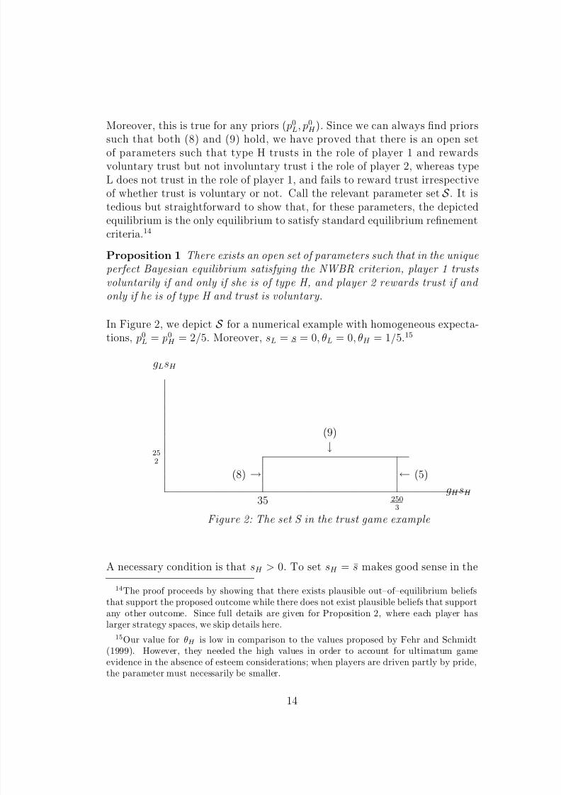
In Figure 2, we depict S for a numerical example with homogeneous expecta-tions, p0L = p0H = 2/5. Moreover, sL = s = 0, θL = 0, θH = 1/5.15

.

.

.

.

.

.

.

.

.

.

.

.

.

.

.

.

.

.

.

.

.

.

.

.

.

.

.

.

.

.

.

.

.

.

.

.

.

.

.

.

.

.

.

.

.

.

.

.

.

.

.

.

.

.

.

.

.

.

.

.

.

.

.

.

.

.

.

.

.

.

.

.

.

.

.

.

.

.

.

.

.

.

.

.

.

.

.

.

.

.

.

.

.

.

.

.

.

.

.

.

.

.

.

.

.

.

.

.

.

.

.

.

.

.

.

.

.

.

.

.

.

.

.

.

.

.

.

.

.

.

.

.

.

.

.

.

.

.

.

.

.

.

.

.

.

.

.

.

.

.

.

.

.

.

.

.

.

.

.

.

.

.

.

.

.

.

.

.

.

.

.

.

.

.

.

.

.

.

.

.

.

.

.

.

.

.

.............

.

.

.

.

.

.

.

.

.

.

.

.

.

.

.

.

.

.

.

.

.

.

.

.

.

.

.

.

.

.

.

.

.

.

.

.

.

.

.

.

.

.

.

.

.

.

.

.

.

.

.

.

.

.

.

.

.

.

.

.

.

.

.

.

.

.

.

.

.

.

.

.

.

.

.

.

.

.

.

.

.

.

.

.

.

.

.

.

.

.

.

.

.

.

.

.

.

.

.

.

.

.

.............................................................................................................................................................................................................................................................................................................................................................................................................................................................................................................................................................................................................................................................................................................................................................................................................................................................................

.

.

.

.

.

.

.

.

.

.

.

.

.

.

.

.

.

.

.

.

.

.

.

.

.

.

.

.

.

.

.

.

.

.

.

.

.

.

.

.

.

.

.

.

.

.

.

.

.

.

.

.

.

.

.

.

.

.

.

.

.

.

.

.

.

.

.

.

.

.

.

.

.

.

.

.

.

.

.

.

.

.

.

.

.

.

.

.

.

.

.

.

.

..........................................................................................................................................................................................................................................................................................................................................................................

Figure 2: The set S in the trust game example

gH sH

gLsH

35 2503

252

→(8)

(9)

↓

← (5)

A necessary condition is that sH > 0. To set sH = s makes good sense in the

14The proof proceeds by showing that there exists plausible out–of–equilibrium beliefsthat support the proposed outcome while there does not exist plausible beliefs that supportany other outcome. Since full details are given for Proposition 2, where each player haslarger strategy spaces, we skip details here.

15Our value for θH is low in comparison to the values proposed by Fehr and Schmidt(1999). However, they needed the high values in order to account for ultimatum gameevidence in the absence of esteem considerations; when players are driven partly by pride,the parameter must necessarily be smaller.

14

8/8/2019 04122006


trust game, because the source of esteem is generosity. As one would expect,

the key to generating the desired equilibrium is then that gL is sufficientlysmall, which guarantees that type L always plays N, while gH takes an inter-mediate value which is large enough to make type H players trust voluntarilyin the role of player 1, but not so large that they reward involuntary trust asplayer 2. Note also that the parameter box in Figure 2 can be made to expandby allowing heterogeneous priors; in particular, a smaller pL expands upwards,and a larger pH expands both sides.

In Appendix 2, we illustrate how the model can similarly be used to explainbehavior in the (mini-) ultimatum game. Here, we proceed to consider ourmain application.

4 The principal-agent relationship

In a principal-agent setting, one player, the principal, first chooses a contractand the other player, the agent, then chooses an effort level. Denote the effortlevel a and let the contract t : A → R specify the agent’s remuneration. Theagent’s effort yields a benefit B(a) to the principal and a cost C (a, θ) to theagent. The cost of the contract to the principal is denoted T (t(a)).

We assume that T (a) ≥ t(a). When the two are equal, t can be thought of as a pure transfer; otherwise the principal pays more than the agent receives

or receives less than the agent pays. In the case that the agent is penalized(t(a) < 0) without the principal being rewarded (T (a) ≥ 0) we can think of the principal engaging in control of the agent’s actions. When nothing else issaid, we assume B(a) is non–negative, increasing and concave, that C (a) iseverywhere twice differentiable and weakly concave in a. We confine attentionto incentive schemes that have at most one “jump”; more precisely, we assumethat t is differentiable everywhere, except possibly for an upward jump at someaction au. In particular, we allow fixed wages with or without firing threats,bonus contracts, and linear incentive schemes.

The key feature of our model, compared to the standard principal–agent

analysis, is that both the agent and the principal engage in signaling. Theagent’s action a is potentially informative of θA and the principal’s contractproposal t(a) is potentially informative of the principal’s characteristics, θP .

For most of the paper, and all of this section, we confine attention to thetwo–type example specified in Section 2.6.

4.1 Selfish players

When players are entirely selfish, any private information concerns monetarycosts and benefits. We shall consider the case in which only the agent’s pro-

15

8/8/2019 04122006


ductivity matters for material payoffs. More precisely, we write the principal’s

utility asU P = B(a) − T (t(a)) + V (ˆ pA(t), θP ), (10)

and the agent’s utility as

U A = t(a) − C (a, θA) + V (ˆ pP (a, t), θA). (11)

Note that (10) implies that the principal cares about how her productivitywill be rated by the agent, even if the principal does not actually work. Wethink that this is realistic in many cases, and it preserves the model’s symmetry,but as will become clear our main results would go through even if we were toneglect the principal’s pride by setting V (ˆ pA(t), θP ) = 0.

4.1.1 The agent’s problem

In this version of the model, the two agent types can be called productive (θH )and unproductive (θL).

The principal’s prior describes a subjective probability p0P that the agentis productive. The probability p0P is drawn from the set { p0L, p0H }.

The contract offer t may carry information about the principal’s type.Thus, pA(t, θI ) denotes the posterior belief about the principal’s type heldby an agent of type I. Likewise, ˆ pP (∅, t , θI ) denotes the posterior belief about

the principal’s prior held by an agent of type I, and ˆ pP (a,t,θI ) denotes theagent’s posterior belief about the principal’s posterior. Recall that it is the ownbelief about the opponent’s posterior beliefs that enters the pride function.

In order for the agent’s signaling problem to be interesting, we assumethat concern for esteem is sufficiently strong to make the unproductive agentcontemplate mimicking the productive agent’s action. (For the moment, weneglect the issue of whether this assumption is consistent with optimal incen-tives t(a).) More precisely, assume that there are unique maximizers

a∗i = arg maxa

[t(a) − C (a, θi)],

and assume that

t(a∗L) − C (a∗L, θL) + V A(0, θL) < t(a∗H ) − C (a∗H , θL) + V A(1, θL), (12)

whereV A(0, θI ) = θL[ pA(θI )sH + (1 − pA(θI ))sL]

is the type I agent’s pride when (he believes that) his type is believed by theprincipal to be L, and

V A(1, θI ) = θH [ pA(θI )sH + (1 − pA(θI ))sL]

16

8/8/2019 04122006


is the pride when (he believes that) his type is believed by the principal to

be H. Obviously, we can always make (12) hold by increasing the differenceθH − θL.

When (12) holds, the productive agent cannot distinguish himself com-pletely through the action a∗H because if this action were sufficient to comeacross as productive, then even the unproductive agent would prefer a∗H to a∗L.We are now ready to state our first result.

Proposition 2 Assume that (i) θ ∈ {θL, θH }; (ii) AA = R+; (iii) t(a) −C (a, θi) have unique maximizers, a∗(θi), and are decreasing in a for a > a∗(θ);(iv) ∂ 2C (a, θ)/∂a∂θ < 0 for all a and θ; (v) the inequality (12) is satisfied.Then, the unique PBE outcome to satisfy NWBR entails actions by the agent,

aL = a∗L and aH = aS H , such that aS H is the solution to

t(a∗L) − C (a∗L, θL) + V A(0, θL) = t(aS H ) − C (aS H , θL) + V A(1, θL). (13)

Proof: See Appendix.

Essentially, Proposition 2 recapitulates the job market signaling argument of Spence (1973). There, productive workers acquire education in order to im-press the prospective future employers; here productive workers put in higheffort so as to impress their current employers. The context is slightly different,but the signaling problem is the same.

Observe that exogenous changes in the material incentives t do not affectimmaterial incentives V at all. Thus, if material incentives are strengthened(for example, through an increase in the slope of t(a)), it follows directlyfrom (13) that aS H must increase. Proposition 2 thus confirms that materialincentives promote effort in the one–sided incomplete information model if agents differ along one dimension only. A similar observation is made byBenabou and Tirole (2006), who go on to investigate what happens whenagents differ along two dimensions.

The first truly novel feature of our model is that the agent’s beliefs aboutthe principal’s type affect the agent’s action. Differentiation of (13) yields

daS H

dpA(θL)=

(θH − θL)(sH − sL)

C (aS H , θL) − t(aS H ). (14)

The denominator is positive under weak assumptions; notably, it is sufficientthat t(a) is concave and C (a, θL) is convex, and at least one of them strictly so.Therefore, the agent’s action is generally increasing in the agent’s optimismregarding the principal’s type. Intuitively, the agent is more keen to make afavorable impression on the type H principal, so the more likely it is that theprincipal is of type H, the more intensively does the type H agent need to work

17

8/8/2019 04122006


in order to credibly signal his type. Our major point, to be elaborated in the

next subsection, is that the principal can use the incentive scheme t not onlyto directly affect the agent’s action (the material incentive effect) but also toaffect it indirectly through the agent’s beliefs (the immaterial incentive effect).

Before turning to the principal’s problem, let us investigate what happenswhen the agent’s actions are bounded above. It is immediately obvious that fullseparation may then no longer be sustainable; when the unproductive agentis willing to take the highest possible action in return for the highest possibleesteem, separation breaks. In a related model, Denrell (1998) suggested thatin this case there would be no signaling; however that conclusion only holdsif we confine attention to pure strategies. There does not seem to be any

justification for doing so here. When mixed strategies are allowed, and theupper bound a is in the interval (a∗L, aS H ), the equilibrium will typically besemi-separating, with type H always choosing the highest feasible action andtype L randomizing between this action and a∗L.

The argument runs as follows. Suppose the type H agent takes an actiona with probability 1. Let x(a) ∈ (0, 1) be the probability with which (theprincipal believes that) the type L agent takes the same action a. Then, theprincipal’s posterior upon seeing a is

pX(a, θI ) =p0(θI )

p0(θI ) + (1 − p0(θI ))x(a). (15)

The equilibrium pride of a type L agent following the action a∗L is V A(0, θL) asbefore. The equilibrium pride of a type L agent following the action a is

V A( pX , θL) = pA(θL)sH [ pX(a, θH )θH + (1 − pX(a, θH ))θL]

+(1 − pA(θL))sL[ pX(a, θL)θH + (1 − pX(a, θL))θL].

Since V A( pX , θL) is monotonically decreasing in x, there can be only one suchsemi–separating equilibrium for a given a. The job of equilibrium refinementsis to rule out equilibria with other supports than (a∗L, a).

Proposition 3 Retain the assumptions of Proposition 2, except replace (ii) by

the assumption sup AA = a < aS H . Then, the unique PBE outcome to satisfy D1 is for type H to play aH = a and for type L to play a with probability x∗

and a∗L with probability (1 − x∗), where x∗ is the solution to

t(a∗L) − C (a∗L, θL) + V A(0, θL) = t(a) − C (a, θL) + V A( pX , θL). (16)


Because of the upper bound, type H is unable to separate completely from typeL, and thus chooses the action that yields the maximum amount of separation,

18

8/8/2019 04122006


i.e., a. Strengthening the monetary incentive serves to increase the equilibrium

fraction x of type L that chooses the high action. Hence, there are no negativeeffects of incentives that are imposed for exogenous reasons.

4.1.2 The principal’s problem

Everything else equal, the principal would like the agent to believe that sheis of type H. There are two reasons: The principal’s own pride and the agentbeing more concerned with the esteem of the type H principal.

If the principal merely claims to be type H, there is no reason why theagent should believe the claim; it can be credible only if the type H principaloffers a contract t that the type L principal prefers not to mimic.

Intuitively, the way for the principal to convince the agent of her hightype is to be generous in case the agent is of type L. The type H principalhas a comparative advantage in being generous to type L agents, becauseof the belief that type L agents are relatively unlikely. Being generous incase of poor performance can be funded by less generosity in case of goodperformance, because the productive agents are kept productive by their fearof being classified as unproductive.

An ambitious objective would be to characterize the principal’s optimalchoice from a large set of incentive schemes. However, this exercise is mean-ingful only if we impose participation or limited liability constraints on the

agent; otherwise the optimal incentive scheme is degenerate. Moreover, thegeneral problem is quite complicated and involves many cases in which imma-terial incentives play a minor role. Therefore, we here only present an examplewhere the set of available material incentive scemes is limited and immaterialincentives come to the forefront.

A high wage as a signal of high expectations

A leading example of trustful contracts is the employment contract thatspecifies a high fixed wage no matter what the worker does. The prevailingexplanation for this finding is that people want to reciprocate; if the principal

behaves kindly, the agent wants to return the favor. (We shall discuss the mer-its of that explanation below.) An alternative explanation emanates from ourmodel with selfish preferences: The best agents work hard when the principalsets a high wage, because the high wage is a credible signal that the principal isproductive and therefore worth impressing. The high wage is a credible signal,because productive principals are more optimistic about their agents.

Here is the formal argument. Suppose the agent’s set of actions A is un-bounded.16 Suppose that the principal can only choose the wage level. That is,

16Our argument goes through with a bounded action set as well, but the formulas are

19

8/8/2019 04122006


t ∈ R+ and T = t. Under our assumption that C (a) is always increasing, i.e.,

the marginal cost of effort is always positive, the unproductive agent will notwork at all due to the lack of pay incentive. That is, aS L = 0. Using equation(13), we see that the productive agent’s effort level aS H ( pA(t, θL)) is given by

C (aS H , θL) = C (0, θL) + (θH − θL)[ pA(θL, t)sH + (1 − pA(θL, t))sL]. (17)

Observe that the payment t has no direct effect on the effort; t only serves tosignal the principal’s type, i.e., to affect pA. As we have already shown, theeffort level aS H is increasing in pA. In order for the type H principal to wantto separate from the type L principal by increasing t, she must have more togain from the expected increase in effort by the type H agent. A sufficient

condition is p0P (θH )B(a) > p0P (θL)B(a), (18)

which holds because the productive principal is more optimistic.

Proposition 4 Suppose the conditions of Propositions 2 hold and determinethe agent’s behavior for fixed agent beliefs. Suppose in addition that: (vi) t(a)can be any constant function, (vii) T = t. Then the unique PBE outcome is for the type L principal to set t = tL = 0 and for the type H principal to set t = tH as the solution to

tH = p0P (θL)B(a

S

H (1)) + V P (1, θL) − V P (0, θL). (19)

Proof: See Appendix.Even if the principal would not care about her own pride, we see from (19)

that the more optimistic principal would signal her high expectations througha high wage. In expectation, she would still earn a positive material surplus[ p0P (θH ) − p0P (θL)]B(aS H (1)).

Our model produces a new twist on the efficiency wage argument. It re-sembles the gift–exchange model of Akerlof (1982). However, Akerlof invokesreciprocity among employers and workers – workers put in more effort when

the wage is high because they want to return the employer’s gift. In Akerlof’swords, workers acquire a sentiment for the firm. Our argument, at least so far,is based on strict selfishness. Productive workers are willing to work harderwhen employers have higher expectations (more optimistic priors), becauseadditional esteem from such “demanding” employers give them more pride.

While our argument may seem far–fetched to some economists, it will befamiliar to many sociologists, psychologists, and business practitioners. Themodel gives a formalization of the self–fulfilling prophecy argument by, among

somewhat different.

20

8/8/2019 04122006


others, Livingston (1969), Archibald (1974) and Eden (1984). All of these

argue that management ought to motivate workers by conveying high, butrealistic, expectations. What we add to their story is that expectations cannotalways be conveyed through words alone. The employer may have to put hermoney where her mouth is and pay high wages as a credible signal of optimism.

4.2 Social preferences

Many of the results with selfish preferences and heterogeneous productivityhave direct counterparts in the case of heterogeneous social preferences. Inparticular, low effort costs are isomorphic to a concern for efficiency.

Following the seminal paper of Fehr, Kirchsteiger and Riedl (1993), severalexperiments have shown that high wages induce high effort. The experimentalevidence typically concern situations in which productivity is known, so therelevant heterogeneity must concern tastes, like altruism, or fairness. The bestcurrent interpretation of the evidence is that the worker wants to reciprocatethe employer’s favor; see Charness (2004). The social preference version of ourmodel offers an alternative interpretation: The employer who offers a high wagesignals high expectations about the worker’s concern for efficiency. Workersvalue esteem from such employers more than esteem from employers with lowexpectations, and hence generous workers put in more effort following a highwage offer than following a low wage offer. The formal argument is isomorphicto that Propositions 2 and 4, so we do not repeat it.

Relabelling the parameter θ as altruism, Proposition 2 offers an explanationfor observable acts of generosity. Indeed our analysis even explains why somepeople give positive and “interior” amounts in the dictatorship game.17 Tosee this, let a be the amount transferred from the agent to the principal andsuppose the principal’s only feasible incentive scheme is t(a) = T (a) = 0.Furthermore, for illustration let B(a, θP ) = a/θP and C (a) = a/θA. Withthese assumptions, a∗L = a∗H = 0, so neither agent type would give anythingabsent a concern for esteem. Since V A(1, θL) > V A(0, θL), (12) holds. FromProposition 2 it then follows that the relative altruists, the type H agents, will

give a strictly positive amount aS H merely to signal their altruism, whereas therelative egoists give nothing.

If instead the parameter θ denotes inequality aversion, the single–crossingcondition in Proposition 2 will no longer hold. Since we believe that concerns

17In the Dictatorship game, one player - the Dictator - has an amount of money and isfree to divide it in any way between herself and a passive recipient. If people are entirelyselfish they should not give anything; if they are generous enough to give something, it ispuzzling that they don’t always give everything (in case of altruism) or exactly half (in caseof inequality aversion), but quite often settle on intermediate amounts.

21

8/8/2019 04122006


for equality are important in many experiments, let us give a general result for

this case.

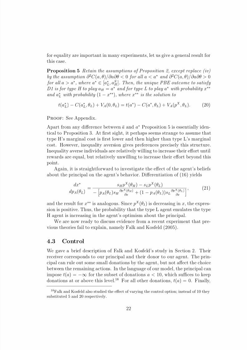
Proposition 5 Retain the assumptions of Proposition 2, except replace (iv)by the assumption ∂ 2C (a, θ)/∂a∂θ < 0 for all a < a∗ and ∂ 2C (a, θ)/∂a∂θ > 0 for all a > a∗, where a∗ ∈ [a∗L, aS H ]. Then, the unique PBE outcome to satisfy D1 is for type H to play aH = a∗ and for type L to play a∗ with probability x∗∗

and a∗L with probability (1 − x∗∗), where x∗∗ is the solution to

t(a∗L) − C (a∗L, θL) + V A(0, θL) = t(a∗) − C (a∗, θL) + V A( pX , θL). (20)


Apart from any difference between a and a∗ Proposition 5 is essentially iden-tical to Proposition 3. At first sight, it perhaps seems strange to assume thattype H’s marginal cost is first lower and then higher than type L’s marginalcost. However, inequality aversion gives preferences precisely this structure.Inequality averse individuals are relatively willing to increase their effort untilrewards are equal, but relatively unwilling to increase their effort beyond thispoint.

Again, it is straightforward to investigate the effect of the agent’s beliefsabout the principal on the agent’s behavior. Differentiation of (16) yields

dx∗

dpA(θL)= sH pX(θH ) − sL pX(θL)

− pA(θL)sH

∂pX(θH)∂x

+ (1 − pA(θL))sL∂pX(θL)

∂x

, (21)

and the result for x∗∗ is analogous. Since pX(θI ) is decreasing in x, the expres-sion is positive. Thus, the probability that the type L agent emulates the typeH agent is increasing in the agent’s optimism about the principal.

We are now ready to discuss evidence from a recent experiment that pre-vious theories fail to explain, namely Falk and Kosfeld (2005).

4.3 Control

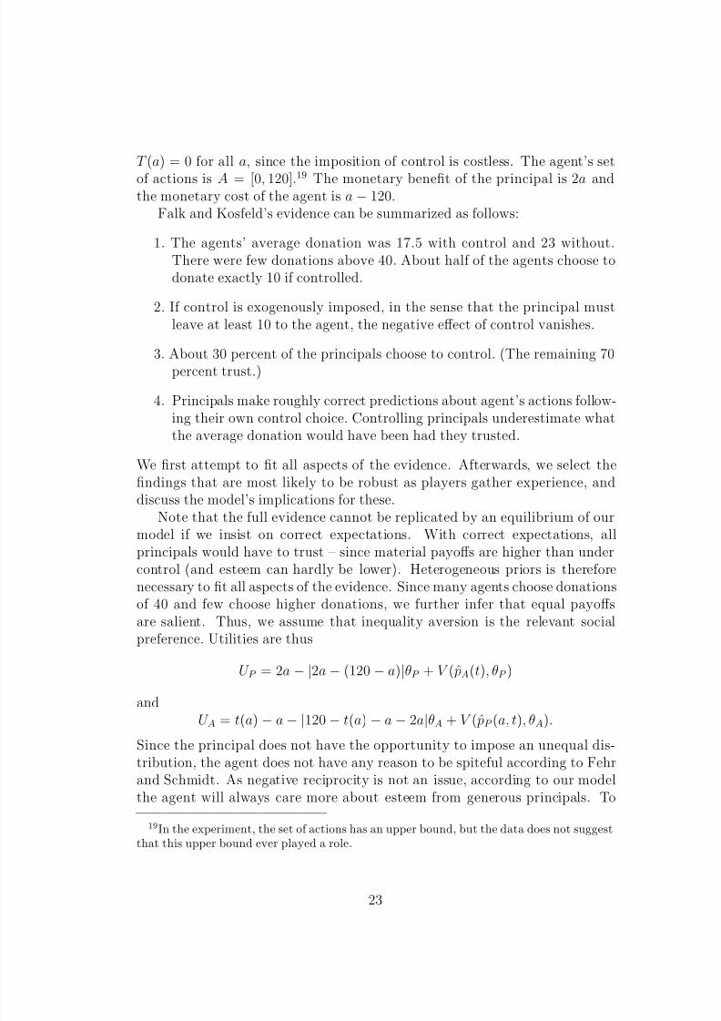
We gave a brief description of Falk and Kosfeld’s study in Section 2. Theirreceiver corresponds to our principal and their donor to our agent. The prin-cipal can rule out some small donations by the agent, but not affect the choicebetween the remaining actions. In the language of our model, the principal canimpose t(a) = −∞ for the subset of donations a < 10, which suffices to keepdonations at or above this level.18 For all other donations, t(a) = 0. Finally,

18Falk and Kosfeld also studied the effect of varying the control option; instead of 10 theysubstituted 5 and 20 respectively.

22

8/8/2019 04122006


T (a) = 0 for all a, since the imposition of control is costless. The agent’s set

of actions is A = [0, 120].19 The monetary benefit of the principal is 2a andthe monetary cost of the agent is a − 120.

Falk and Kosfeld’s evidence can be summarized as follows:

1. The agents’ average donation was 17.5 with control and 23 without.There were few donations above 40. About half of the agents choose todonate exactly 10 if controlled.

2. If control is exogenously imposed, in the sense that the principal mustleave at least 10 to the agent, the negative effect of control vanishes.

3. About 30 percent of the principals choose to control. (The remaining 70percent trust.)

4. Principals make roughly correct predictions about agent’s actions follow-ing their own control choice. Controlling principals underestimate whatthe average donation would have been had they trusted.

We first attempt to fit all aspects of the evidence. Afterwards, we select thefindings that are most likely to be robust as players gather experience, anddiscuss the model’s implications for these.

Note that the full evidence cannot be replicated by an equilibrium of our

model if we insist on correct expectations. With correct expectations, allprincipals would have to trust – since material payoffs are higher than undercontrol (and esteem can hardly be lower). Heterogeneous priors is thereforenecessary to fit all aspects of the evidence. Since many agents choose donationsof 40 and few choose higher donations, we further infer that equal payoffsare salient. Thus, we assume that inequality aversion is the relevant socialpreference. Utilities are thus

U P = 2a − |2a − (120 − a)|θP + V (ˆ pA(t), θP )

and

U A = t(a) − a − |120 − t(a) − a − 2a|θA + V (ˆ pP (a, t), θA).

Since the principal does not have the opportunity to impose an unequal dis-tribution, the agent does not have any reason to be spiteful according to Fehrand Schmidt. As negative reciprocity is not an issue, according to our modelthe agent will always care more about esteem from generous principals. To

19In the experiment, the set of actions has an upper bound, but the data does not suggestthat this upper bound ever played a role.

23

8/8/2019 04122006


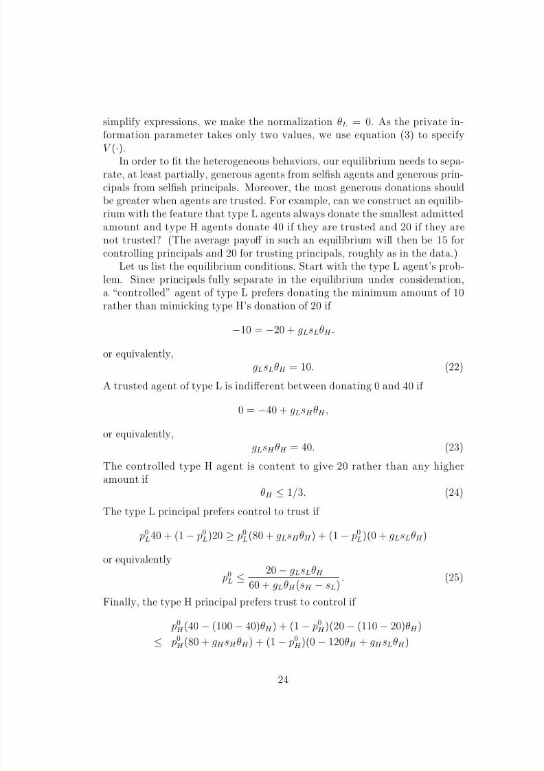
simplify expressions, we make the normalization θL = 0. As the private in-

formation parameter takes only two values, we use equation (3) to specifyV (·).

In order to fit the heterogeneous behaviors, our equilibrium needs to sepa-rate, at least partially, generous agents from selfish agents and generous prin-cipals from selfish principals. Moreover, the most generous donations shouldbe greater when agents are trusted. For example, can we construct an equilib-rium with the feature that type L agents always donate the smallest admittedamount and type H agents donate 40 if they are trusted and 20 if they arenot trusted? (The average payoff in such an equilibrium will then be 15 forcontrolling principals and 20 for trusting principals, roughly as in the data.)

Let us list the equilibrium conditions. Start with the type L agent’s prob-lem. Since principals fully separate in the equilibrium under consideration,a “controlled” agent of type L prefers donating the minimum amount of 10rather than mimicking type H’s donation of 20 if

−10 = −20 + gLsLθH .

or equivalently,gLsLθH = 10. (22)

A trusted agent of type L is indifferent between donating 0 and 40 if

0 = −40 + gLsH θH ,

or equivalently,gLsH θH = 40. (23)

The controlled type H agent is content to give 20 rather than any higheramount if

θH ≤ 1/3. (24)

The type L principal prefers control to trust if

p

0

L40 + (1 − p

0

L)20 ≥ p

0

L(80 + gLsH θH ) + (1 − p

0

L)(0 + gLsLθH )

or equivalently

p0L ≤20 − gLsLθH

60 + gLθH (sH − sL). (25)

Finally, the type H principal prefers trust to control if

p0H (40 − (100 − 40)θH ) + (1 − p0H )(20 − (110 − 20)θH )

≤ p0H (80 + gH sH θH ) + (1 − p0H )(0 − 120θH + gH sLθH )

24

8/8/2019 04122006


or equivalently

p0H > 20 + 120θH − gH sLθH

60 + 90θH + gH θH (sH − sL)(26)

Observe that the right hand side is decreasing in gH . Since gH ≥ gL, wecan replace gH by gL to get an upper bound. If we set θH = 1/5 as before,the last two conditions then become p0L ≤ 1/9 and p0H ≥ 2/99. Only thefirst condition is restrictive. Our example thus mimicks the main features of Falk and Kosfeld’s evidence if we are willing to allow type L agents to besufficiently (over)pessimistic.20 Moreover, under the assumed parameters it isstraightforward to check that the proposed equilibrium uniquely survive therefinement criteria that we have imposed.

When asked about their reaction to the principal’s decision to control them,subjects who reduce their donations express feelings of being restricted anddistrusted (Falk and Kosfeld, Figure 2). Our model captures this phenomenoninasmuch as both types of agents would prefer to be trusted. This is mostobvious for the type L agent, who loses 10 without any compensation in termsof pride when controlled. The type H agent keeps more money when controlled,but the monetary gain is more than offset by a reduced sense of pride.

Finally, let us consider what happens when control is exogenously imposedrather than chosen by the principal. The exogenous control treatment imple-mented by Falk and Kosfeld essentially limits the action set of the agent to

[10, 120]. (They do not use the word “control” in the instructions to the subjects. As we shall see below, wording could affect the results.) Recall that thedonation of type H agents is given by the need to separate from type L agents.Given that the agent has no information about the principal, the separatingequilibrium condition pinning down the type H agent’s donation becomes

−10 = −aH + gLθH ( p0LsH + (1 − p0L)sL).

Recall that under endogenous control, due to full separation of principal types,the condition was

−10 = −aH + gLθH sL.

The solution (aH ) must be larger when control is exogenous than when itis endogenous, because sH > sL. When control is endogenous, the agent

20The example does not quite mimick the fact that controlling principals in the experimenthave correct expectations about controlled agents’ average donations; in the example, theprediction is (8/9) · 10+(1/9) · 20 which is smaller than the average donation of 15. Also, thefraction of principals who trust in the example (one half) is smaller than the fraction whotrust in the experiment (three quarters). On both these counts we can improve the model’sfit by considering a semi-separating equilibrium, in which type L principals are indifferentbetween trusting and controlling.

25

8/8/2019 04122006


8/8/2019 04122006


4.4 Penalties and trust

Gneezy and Rustichini (2000a) conduct a field experiment in which severaldaycare centers are induced to impose a fine on parents who collect theirchildren too late in the evening. The effect of the fine is to increase theprevalence of late collection. When the penalty is removed, parents continue tocollect their children later than before. Thus, a good theory needs to explainboth why the fine backfires to begin with and why behavior does not revertwhen the fine is removed.

Our model offers explanations for both findings. Without the fine, thedaycare manager displayed trust, and parents attempted to collect children intime in order to gain the manager’s approval. The imposition of fines signal a

reduction in trust, which implies that the value of approval declines. If the fineis relatively small, parents will behave less diligently. If the fine is seen to beremoved because it did not work, rather than because the manager suddenlytrusts the parents again, the parents will continue their less diligent ways –indeed, they should become even less diligent than before, because the esteemincentive and the pecuniary incentive are both gone.

Two recent studies by Fehr and Rockenbach (2003) and Fehr and List(2004) consider a version of the trust game, but with two twists: The trustor al-ways states a desired back-transfer, and the trustor can choose upfront whetherto punish a smaller-than-desired back-transfer by imposing a fine. Concretely,

the trustor has 10 money units. For every unit given, the trustee receives 3units. (Thus, the best egalitarian outcome is for the trustor to give all 10 andfor the trustee to make a back-transfer of 20.) The fine is 4 money units, andif the fine kicks in these units are wasted - not transfered to the trustor. Amain finding is that the decision by the trustor to impose a fine leads to lowerback-transfers, so trustors are better off by foregoing the punishment option.It is straightforward to demonstrate that our model rationalizes the behavior:The imposition of the fine signals low expectations, thereby reducing the valueof esteem. As a result of the fine, the smallest donations go up, but the largestdonations go down.

4.5 Framing

Framing has a significant effect on behavior in many games. As shown byLiberman, Samuels and Ross (2004), people’s actions in the prisoners’ dilemmagame depend heavily on whether experimenters call it the Community Game orthe Wall Street Game.22 A natural explanation is that concern for cooperation

22For a seminal contribution along the same lines, see Eiser and Bhavnani (1974). Seealso Pillutla and Chen (1999) and Rege and Telle (2003) for closely related work.

27

8/8/2019 04122006


is more salient in the “community” than on Wall Street. Our model is able

to capture variation in salience through the salience weights s. All we needto do is to specify a mapping from the set of decision frames to the set of salience weights. In doing so, we may borrow heavily from research in socialpsychology, which has devoted considerable effort to the classification of socialframes; see for example Levin et al.(1998).

Recently, several experiments have studied the effect of framing on incen-tives. Fehr and Gachter (2002) investigate the role of fines in a gift exchangeexperiment. The principal commits to a wage and states a desired effort level,but can also choose a wage combined with a fine – to be imposed if the agent’seffort is discovered to be lower than desired (the principal can observe the effort

with some probability smaller than 1). The contract with a fine tend to entaillower effort for a given wage level, much as we might expect by now. However,when the authors rephrase the experiment, so that the principal chooses eithera plain wage or a plain wage combined with a bonus in case the agent exertsthe desired effort (or, more precisely, is not discovered to be shirking), theincentive works considerably better. Note that the two treatments give theprincipal exactly the same set of options: A wage of w coupled with a fine f is equivalent to a wage of w − f coupled with a bonus of f . So why does thelatter contract work better? Since the only difference is in the words “bonus”and “fine”, we posit that these words must trigger different associations.

Houser et al.(2005) replicate the experiment of Fehr and Rockenbach (2003),but include a treatment in which the punishment threat is random and be-yond the control of the principal. They find that the imposition of (weak)punishment threats have a negative effect on the agent regardless of whetherthe principal imposes it voluntarily or it is imposed randomly. The authorssuggest that the punishment threat induces a cognitive shift away from coop-erative behavior. In the terms of our model, cooperation becomes less salient.

Irlenbusch and Sliwka (2005) document a similar effect. The mere oppor-tunity of paying a piece rate in a gift exchange experiment lowers the agent’seffort. As in the daycare experiment of Gneezy and Rustichini, the detrimen-tal effect of incentives prevail after the incentive is removed; when the trust

game is played again without availability of piece rates, agents display lessreciprocity than when piece rates were never available.

4.6 Other issues

Let us here briefly mention some issues that we have neglected so far.

28

8/8/2019 04122006


4.6.1 Incentives affect the principal’s desires

Up until now, we assumed that principals always appreciate “good” charac-teristics. However, credit card companies do not ordinarily want customers topay their debts on time. As long as customers pay eventually, the high interestrate make the companies better off when the customers pay late. Because of the incentive scheme, the principal wants to encourage sloppy payment prac-tices rather than diligence. As a result, there is no reason for the customers tofeel appreciated by the credit card company when paying on time.

The daycare experiment can perhaps be interpreted in this way too. Tothe extent that the imposition of a fine indicates that the daycare center isnow indifferent towards parents’ behavior (or even prefers late collection), why

should parents take pride in punctuality? It seems to us that the salienceweight on the punctuality parameter ought to be zero in this case.

4.6.2 Multiple tasks: incentives as communication

We have assumed that the agent’s effort is unidimensional and the principal’sobjective is publicly known. In many realistic cases effort is multi-dimensional,and the principal’s objective is privately known.

Suppose for a moment that agents do not know what behaviors are inthe principal’s interest, but do know the principal’s expectations about agent

characteristics. It is now possible that agents’ behavior reacts strongly tosmall but informative clues, with little or no material payoff relevance to theagents. For example, small bonuses - and even gold stars and other materiallyworthless distinctions - can be used to indicate which behaviors are deemedto be desirable. A bonus based on group performance indicates that concernfor others’ output is valued; bonuses based on individual performance indicatethat concern for others is less important. Small rewards play the essentiallysame role as verbal communication. If rewards are increased, a reasonableinterpretation is now that high effort is more valuable to the principal thanbefore. In this case, there is a positive incentive multiplier: The direct effectthrough higher material reward is complemented by an indirect effect throughincreased salience of high effort for esteem purposes.

4.6.3 Multiple observers

In our principal–agent examples, we have so far assumed that the principalplays three roles: She designs the contract, is the beneficiary of agent coop-eration, and is the sole observer whom the agent may impress. One way todistinguish the predictions of our model from the predictions of reciprocitymodels is to separate these three roles. For example, reciprocity models pre-

29

8/8/2019 04122006


dict that the agent will be kind in order to reward kindness, whereas our model

predicts that the agent is kind in order to impress an audience.

5 Final remarks

The analysis can be extended in several directions. We think that it mightexplain why people dislike being monitored, and why this dislike is strongerwhen monitoring is linked to future rewards, as demonstrated by Enzle andAnderson (1993). It might also be able to explain why careful ex ante planningby one contracting party “indicates a lack of trust and blunts the demands of friendship” as suggested by Macaulay (1963, p64). Finally, it is natural to

explore the nature of optimal incentive schemes under the assumption thatpeople care about esteem. Our preliminary investigations suggest that a fixedwage can be optimal under quite plausible assumptions.

All this is not to say that material incentives never work, or even thatthe case for material incentives is weaker than the traditional principal–agentmodel suggests. In order to explain a set of puzzles, we have been led toconsider cases in which esteem incentives are naturally aligned with the prin-cipal’s interest. Recognizing that agents may seek esteem from others thanthe principal, the presence of esteem incentives could well strengthen the casefor material incentives. For example, asking a CEO to engage in heavy cost

cutting could be extremely difficult if the CEO cares more about esteem fromthe firm’s employees than from the firm’s owners. We believe that this is onereason why corporate restructuring either has to wait until employees are suffi-ciently “crisis conscious” or is carried out by a new manager on strong materialincentives, who often leaves when the job is done.

Finally, our model of human nature can be applied to analyze many othersocial settings than those we have considered here.

Appendix 1: Proofs

All the proofs are standard applications of the NWBR and D1 criteria. Infact, since senders care directly about receivers’ beliefs rather than about thereceiver’s rational actions following these beliefs, the notation is somewhatsimpler than usual.

Proof of Proposition 2

From condition (iv) it follows that a∗L ≤ a∗H , with equality only if a∗H = au

(type H’s favorite outcome is at a point where the material incentives jump

30

8/8/2019 04122006


upwards). From (iv) and (12) it follows that aS H > a∗H . Conditions (ii) and

(iii) together with differentiability of C and t (except for possibly one upward jump) ensure that aS H exists and is unique.

Next, we check that there exist “reasonable” out–of–equilibrium beliefs thatsustain the proposed equilibrium outcome: Let the principal believe that anyaction a < aS H is taken by a type L agent. Then, by definition, a∗L dominatesall actions a ∈ (a∗L, aS H ) for type L. Since aS H dominates all actions a > aS H

for type L, it follows from (13) that L has no incentive to deviate from a∗L. Tocheck that type H has nothing to gain from deviating from aS H , observe thatany higher action entails lower utility, and that the best lower action is a∗H .Type H prefers aS H to a∗H if

t(a∗H ) − C (a∗H , θH ) + V A(0, θH ) < t(aS H ) − C (aS H , θH ) + V A(1, θH ). (27)

Observe that V A(1, θI ) − V A(0, θI ) = [ pA(θI )sH + (1 − pA(θI ))sL][θH − θL]for I ∈ {L, H }. Since pA(θH ) ≥ pA(θL) it follows that V A(1, θH ) − V A(0, θH ) ≥V A(1, θL) − V A(0, θL). It is thus sufficient to show that (27) is satisfied whenV A(1, θH ) − V A(0, θH ) = V A(1, θL) − V A(0, θL). Substituting for t(aS H ) from (13)and rearranging, the condition then becomes

C (aS H , θH ) − C (a∗H , θH ) < C (aS H , θL) − C (a∗L, θL) + t(a∗L) − t(a∗H ). (28)

Since a∗L is the unique solution to type L’s problem, t(a∗L)−C (a∗L, θL) > t(a∗H )−C (a∗H , θL), or equivalently, t(a∗L) − t(a∗H ) ≥ C (a∗L, θL) − C (a∗H , θL). Thus, theright hand side of (28) cannot be smaller than C (aS H , θL) − C (a∗L, θL). In otherwords, aS H is a best response for type H if

C (aS H , θH ) − C (a∗H , θH ) < C (aS H , θL) − C (a∗L, θL),

and this inequality is fulfilled due to the single–crossing condition (iv). Thus,we have proved that the beliefs sustain the proposed equilibrium strategies.To see that the principal’s beliefs are reasonable out of equilibrium, note thata deviation by type L to an action in the interval (a∗L, a∗H ) would be justifiedif the principal were to believe that the action was taken by a type H agent.Thus, the belief that any such deviation is due to a type L player satisfies theNWBR-property.

The final step is to show that all other perfect Bayesian equilibria fail theNWBR property. Consider first other fully separating equilibria. We knowthat these entail aL = a∗L and aH > aS H . In order for type H not to deviateto a lower action (which, by condition (iii) gives higher utility if beliefs areconstant), the principal must believe that there is some probability that thislower action is taken by a type L agent. But by condition (iii) and equation(13) type L is always worse off taking an action a > aS H than with a∗L. Thus,

31

8/8/2019 04122006


the principal’s belief fails NWBR. Consider next any pooling equilibrium aL =

aH = a∗

. To destroy it, show that there exists an action ad > a∗

which is suchthat type H is willing to deviate to ad if the principal becomes convinced thatthe agent’s type is H, but type L is not willing to make the deviation regardlessof the principal’s beliefs. (Finding ad is analogous to finding aS H , again single–crossing is the key, so we do not repeat the step.) Since type H can only bedeterred from deviating to ad if the principal ascribes a positive probability tothe deviation being caused by a type L agent, the pooling equilibrium belief must fail NWBR. Finally, consider semi–separating equilibria, where there isat least one action as that both types play with positive probability. Again,this equilibrium can be destroyed by identifying a deviation that is potentially

attractive only to type H.


Most of the proof is analogous to the proof of Proposition 1, so we are brief:First show that there are out–of–equilibrium beliefs that sustain the proposedoutcome as a PBE. In particular, suppose that the principal believes that anyaction a ∈ (a∗L, a) is taken by a type L agent. Clearly, all actions a ∈ (a∗L, a)are then dominated by a∗L. Given that the Principal updates the prior usingBayes’ rule, the probability assigned to type H given action a is pX . Thus,if (16) holds, type L is indifferent between actions a∗L and a. Since type Hhas lower marginal cost of effort than type L, and at least as much to gain byraising V A from V A(1, ·) to V A( pX , ·), it follows that type H strictly prefers ato all other available actions given the assumed beliefs. Thus, we have indeeddescribed a PBE. The equilibrium satisfies D1, because there is a larger setof (alternative) beliefs that would justify any action a ∈ (a∗L, a) by the typeL agent than by the type H agent. It remains to check that no other PBEsurvives D1. Consider any equilibrium in which there is some partial poolingat an action a∗ < a. This equilibrium must be sustained by “sufficientlypessimistic” beliefs following a deviation to all higher actions (otherwise, typeH would deviate). But due to the single–crossing conditions on C and V A,

the set of beliefs justifying a deviation to a by type H is again larger thanthe corresponding set for type L. Thus, by D1, the principal must ascribe thedeviation to a type H player, contradicting the original pessimistic beliefs.


Most of the proof is analogous to the proof of Proposition 3. The main differ-ence is that we also need to consider equilibria with partial pooling at someaction a > a∗. These equilibria fail D1 because they must assume relatively

32

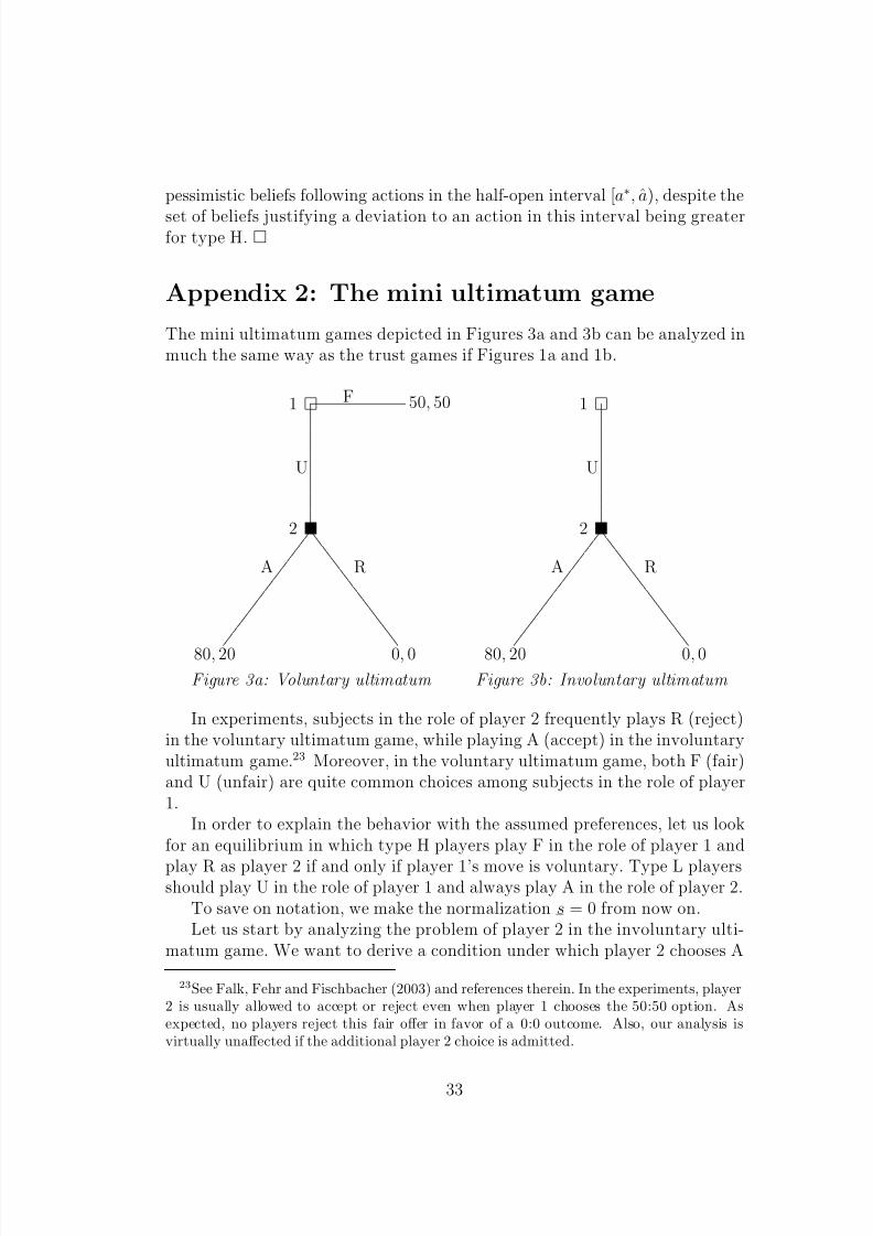
8/8/2019 04122006


pessimistic beliefs following actions in the half-open interval [a∗, a), despite the

set of beliefs justifying a deviation to an action in this interval being greaterfor type H.

Appendix 2: The mini ultimatum game

The mini ultimatum games depicted in Figures 3a and 3b can be analyzed inmuch the same way as the trust games if Figures 1a and 1b.

1

2

50, 50

80, 20 0, 0

1

2

80, 20 0, 0

F

U

A R

U

A R

Figure 3a: Voluntary ultimatum Figure 3b: Involuntary ultimatum

........................................................................................................................................................

.

.

.

.

.

.

.

.

.

.

.

.

.

.

.

.

.

.

.

.

.

.

.

.

.

.

.

.

.

.

.

.

.

.

.

.

.

.

.

.

.

.

.

.

.

.

.

.

.

..............

.

.

.

.

.

.

.

.

.

.

.

.

.

.

.

.

.

.

.

.

.

.

.

.

.

.

.

.

.

.

.

.

.

.

.

.

.

.

.

.

.

.

.

.

.

.

.

.

.

.

.

.

.

.

.

.

.

.

.

.

.

.

.

.

.

.

.

.

.

.

.

.

.

.

.

.

.

.

.

.

.

.

.

.

.

.

.

.

.

.

.

.

.

.

.

.

.

.

.

.

.

.

.

.

.

.

.

.

.

.

.

.

.

.

.

.

.

.

.

.

.

.

.

.

.

.

.

.

.

.

.

.

.

.

.

.

.

.

.

.

.

.

.

.

.

.

.

.

..

.....................................................................................................................................................................................................................................................

.

.......................................................................................................................................................................................................................................................

.

.

.

.

.

.

.

.

.

.

.

.

.

.

.

.

.

.

.

.

.

.

.

.

.

.

.

.

.

.

.

.

.

.

.

.

.

.

.

.

.

.

.

.

.

.

.

.

.

.

..............

.

.

.

.

.

.

.

.

.

.

.

.

.

.

.

.

.

.

.

.

.

.

.

.

.

.

.

.

.

.

.

.

.

.

.

.

.

.

.

.

.

.

.

.

.

.

.

.

.

.

.

.

.

.

.

.

.

.

.

.

.

.

.

.

.

.

.

.

.

.

.

.

.

.

.

.

.

.

.

.

.

.

.

.

.

.

.

.

.

.

.

.

.

.

.

.

.

.

.

.

.

.

.

.

.

.

.

.

.

.

.

.

.

.

.

.

.

.

.

.

.

.

.

.

.

.

.

.

.

.

.

.

.

.

.

.

.

.

.

.

.

.

.

.

.

.

.

.

.......................................................................................................................................................................................................................................................

.

.......................................................................................................................................................................................................................................................

In experiments, subjects in the role of player 2 frequently plays R (reject)in the voluntary ultimatum game, while playing A (accept) in the involuntaryultimatum game.23 Moreover, in the voluntary ultimatum game, both F (fair)and U (unfair) are quite common choices among subjects in the role of player1.

In order to explain the behavior with the assumed preferences, let us lookfor an equilibrium in which type H players play F in the role of player 1 and

play R as player 2 if and only if player 1’s move is voluntary. Type L playersshould play U in the role of player 1 and always play A in the role of player 2.

To save on notation, we make the normalization s = 0 from now on.Let us start by analyzing the problem of player 2 in the involuntary ulti-

matum game. We want to derive a condition under which player 2 chooses A

23See Falk, Fehr and Fischbacher (2003) and references therein. In the experiments, player2 is usually allowed to accept or reject even when player 1 chooses the 50:50 option. Asexpected, no players reject this fair offer in favor of a 0:0 outcome. Also, our analysis isvirtually unaffected if the additional player 2 choice is admitted.

33

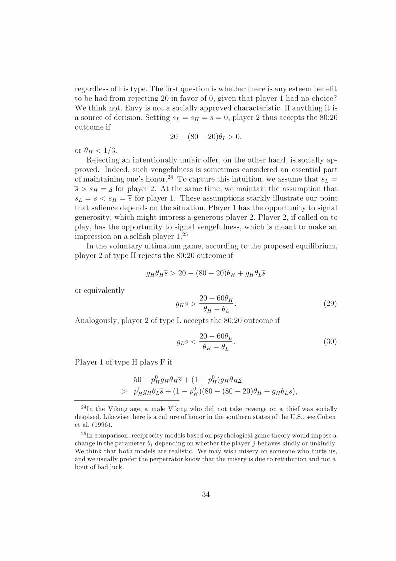
8/8/2019 04122006


regardless of his type. The first question is whether there is any esteem benefit

to be had from rejecting 20 in favor of 0, given that player 1 had no choice?We think not. Envy is not a socially approved characteristic. If anything it isa source of derision. Setting sL = sH = s = 0, player 2 thus accepts the 80:20outcome if

20 − (80 − 20)θI > 0,

or θH < 1/3.Rejecting an intentionally unfair offer, on the other hand, is socially ap-

proved. Indeed, such vengefulness is sometimes considered an essential partof maintaining one’s honor.24 To capture this intuition, we assume that sL =s > sH = s for player 2. At the same time, we maintain the assumption that

sL = s < sH = s for player 1. These assumptions starkly illustrate our pointthat salience depends on the situation. Player 1 has the opportunity to signalgenerosity, which might impress a generous player 2. Player 2, if called on toplay, has the opportunity to signal vengefulness, which is meant to make animpression on a selfish player 1.25

In the voluntary ultimatum game, according to the proposed equilibrium,player 2 of type H rejects the 80:20 outcome if

gH θH s > 20 − (80 − 20)θH + gH θLs

or equivalently

gH s >20 − 60θH

θH − θL. (29)

Analogously, player 2 of type L accepts the 80:20 outcome if

gLs <20 − 60θL

θH − θL. (30)

Player 1 of type H plays F if

50 + p0H gH θH s + (1 − p0H )gH θH s

> p0H gH θLs + (1 − p

0H )(80 − (80 − 20)θH + gH θLs),

24In the Viking age, a male Viking who did not take revenge on a thief was sociallydespised. Likewise there is a culture of honor in the southern states of the U.S., see Cohenet al. (1996).

25In comparison, reciprocity models based on psychological game theory would impose achange in the parameter θi depending on whether the player j behaves kindly or unkindly.We think that both models are realistic. We may wish misery on someone who hurts us,and we usually prefer the perpetrator know that the misery is due to retribution and not about of bad luck.

34

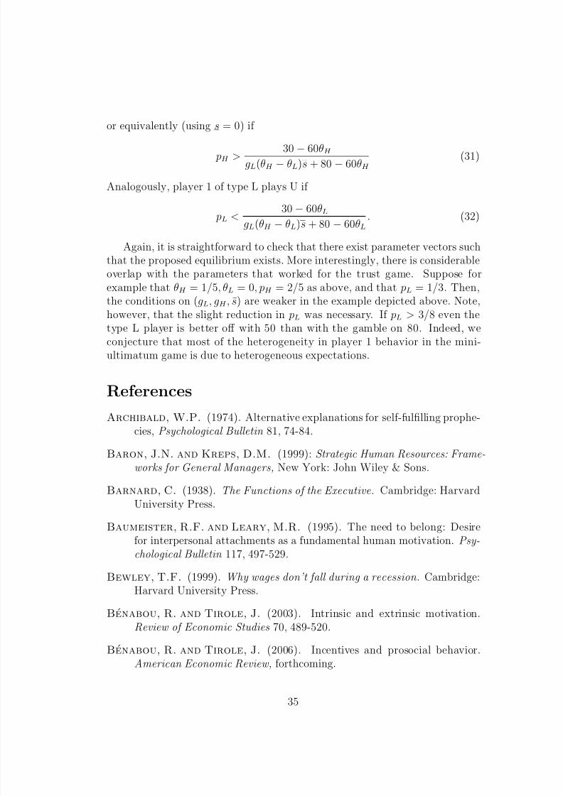
8/8/2019 04122006


or equivalently (using s = 0) if

pH >30 − 60θH

gL(θH − θL)s + 80 − 60θH

(31)

Analogously, player 1 of type L plays U if

pL <30 − 60θL

gL(θH − θL)s + 80 − 60θL. (32)

Again, it is straightforward to check that there exist parameter vectors suchthat the proposed equilibrium exists. More interestingly, there is considerable

overlap with the parameters that worked for the trust game. Suppose forexample that θH = 1/5, θL = 0, pH = 2/5 as above, and that pL = 1/3. Then,the conditions on (gL, gH , s) are weaker in the example depicted above. Note,however, that the slight reduction in pL was necessary. If pL > 3/8 even thetype L player is better off with 50 than with the gamble on 80. Indeed, weconjecture that most of the heterogeneity in player 1 behavior in the mini-ultimatum game is due to heterogeneous expectations.

References

Archibald, W.P. (1974). Alternative explanations for self-fulfilling prophe-cies, Psychological Bulletin 81, 74-84.

Baron, J.N. and Kreps, D.M. (1999): Strategic Human Resources: Frame-works for General Managers, New York: John Wiley & Sons.

Barnard, C. (1938). The Functions of the Executive. Cambridge: HarvardUniversity Press.

Baumeister, R.F. and Leary, M.R. (1995). The need to belong: Desirefor interpersonal attachments as a fundamental human motivation. Psy-

chological Bulletin 117, 497-529.

Bewley, T.F. (1999). Why wages don’t fall during a recession. Cambridge:Harvard University Press.

Benabou, R. and Tirole, J. (2003). Intrinsic and extrinsic motivation.Review of Economic Studies 70, 489-520.

Benabou, R. and Tirole, J. (2006). Incentives and prosocial behavior.American Economic Review, forthcoming.

35

8/8/2019 04122006


Bernheim, D.B. (1994): A theory of conformity. Journal of Political Econ-

omy 102, 841-877.

Bohnet, I., Frey, B.S. and Huck, S. (2001). More order with less law.American Political Science Review 95, 131-144.

Brennan, G. and P. Pettit (2004). The Economy of Esteem. Oxford:Oxford University Press.

Camerer, C.F. (2003). Behavioral Game Theory: Experiments in StrategicInteraction. Princeton: Princeton University Press.

Charness, G. and Rabin, M. (2002). Understanding social preferences withsimple tests. Quarterly Journal of Economics 117, 817-869.

Charness, G, and Dufwenberg, M (2005). Promises and partnership,Econometrica, forthcoming.

Cho, I.-k. and Kreps, D.M. (1987): Signaling games and stable equilib-ria. Quarterly Journal of Economics 50, 179–221.

Coletti, A.L., Sedatole, K.L., and Towry, K.L (2005). The effect of control systems on trust and cooperation in collaborative environments.Accounting Review 80, 477-500.

Dawes, R.M. (1989). Statistical criteria for establishing a truly false con-sensus effect, Journal of Experimental Social Psychology 25, 1-17.

Deci, E.L. (1971). The effects of externally mediated rewards on intrinsicmotivation, Journal of Personality and Social Psychology 18, 105-115.

Deci, E.L., Koestner, R.M. and Ryan, R. (1999). A meta-analytic re-view of experiments examining the effects of extrinsic rewards on intrinsicmotivation Psychological Bulletin 125, 627-668.

Denrell, J. (1998). Incentives and Hypocrisy. Chapter 2 in the PhD dis-sertation Essays on the economics of vanity and career concerns. Stock-holm: Stockholm School of Economics.

Eden, D. (1984). Self-fulfilling prophecy as a management tool: HarnessingPygmalion, Academy of Management Review 9, 64-73.

Eiser, J.R. and K. Bhavnani (1974). The effect of situational meaningon the behavior of subjects in the Prisoners’ Dilemma game, European Journal of Social Psychology 4, 93-97.

36

8/8/2019 04122006


Ellingsen, T. and Johannesson, M. (2005). Trust as an incentive, mimeo.,

Stockholm School of Economics

Engelmann, D. and Strobel, M. (2004): The false consensus effect: De-construction and reconstruction of an anomaly, mimeo.

Enzle, M.E. and S.C. Anderson (1993). Surveillant intentions and in-trinsic motivation. Journal of Personality and Social Psychology 64,257-266.

Falk, A. and Kosfeld, M. (2005). Distrust - the hidden cost of control.American Economic Review, forthcoming. (Originally IEW Working Pa-

per No. 193, University of Zurich.)

Fehr, E. and Rockenback, B. (2003). Detrimental effects of sanctions onhuman altruism,Nature 422, 137-140.

Fehr, E. and Gachter, S. (2002). Do incentive contracts undermine vol-untary cooperation? Working Paper No. 34, Institute for EmpiricalResearch in Economics, University of Zurich.

Fehr, E., Kirchsteiger, G. and Riedl, A. (1993). Does fairness pre-vent market clearing? An experimental investigation. Quarterly Journal

of Economics 108, 437-459.Fehr, E. and List, J. (2004). The hidden costs and returns of incentives

- trust and trustworthiness among CEOs, Journal of the European Eco-nomic Association 2, 743-771.

Fehr, E. and Schmidt, K.M. (1999). A theory of fairness, competition,and cooperation. Quarterly Journal of Economics 114, 817-868.

14,

Frey, B.S. (1993): Does monitoring increase work effort? The rivalry with

trust and loyalty. Economic Inquiry 31, 663-670.Frey, B.S. (1997). Not Just for the Money. An Economic Theory of Per-

sonal Motivation. Cheltenham: Edward Elgar.

Frey, B.S. and Oberholzer-Gee, F. (1997). The cost of price incen-tives: an empirical analysis of motivation crowding out. American Eco-nomic Review 87, 746-755.

37

8/8/2019 04122006


Frey, B.S., Oberholzer-Gee, F. and Eichenberger (1996). The old

lady visits your backyard: a tale of morals and markets. Journal of Political Economy 104, 1297-1313.

Fudenberg, D. and Tirole, J. (1991). Game Theory , Cambridge: MITPress.

Geanakopolos, J, Pearce, D, and Stacchetti, E. (1989). Psycholog-ical games and sequential rationality, Games and Economic Behavior 1,60-79.

Gneezy, U. (2003). Do high wages lead to high profits? An experimen-

tal study of reciprocity using real effort. Mimeo, University of ChicagoGraduate School of Business.

Gneezy, U. and Rustichini, A. (2000a). A fine is a price. Journal of Legal Studies 29, 1-17.

Gneezy, U. and Rustichini, A. (2000b). Pay enough or don’t pay at all.Quarterly Journal of Economics 115, 791-810.

Houser, D., Xiao, E., McCabe, K., and Smith, V. (2005): When pun-ishment fails: Research on sanctions, intentions and non-cooperation,

mimeo., George Mason University.Hume, D. A Treatise of Human Nature, London: John Noon.

Irlenbusch, B., and Sliwka, D. (2005): Incentives, decision frames, andmotivation crowding out - an experimental investigation, IZA DiscussionPaper No. 1758.

Kreps, D. (1997). Intrinsic motivation and extrinsic incentives. American Economic Review, Papers and Proceedings 87, 359-364.

Levin, I.P. et al. (1998). All frames are not created equal: A typology and

critical analysis of framing effects, Organizational Behavior and Human Decision Processes 76, 149-188.

Levine, D.K. (1998). Modeling altruism and spitefulness in experiments,Review of Economic Dynamics 1, 593–622.

Liberman, V., Samuels, S.M. and Ross, L. (2004). The name of the game:Predictive power of reputations versus situational labels in determiningprisoner’s dilemma game moves. Personality and Social Psychology Bul-letin 30, 1175-1185.

38

8/8/2019 04122006


Livingston, J.S. (1969). Pygmalion in management. Harvard Business Re-

view 47 (July–August), 81–89.

Macaulay, S. (1963): Non-contractual relations in business: A preliminarystudy. Americal Sociological Review 28, 55-70.

McCabe, K.A., Rigdon, M.L. and Smith, V.L. (2003): Positive reciprocityand intentions in trust games, Journal of Economic Behavior and Orga-nization 52, 267-275.

McGregor, D. (1960): The Human Side of Enterprise, New York: McGraw-Hill.

Maslow, A.H. (1943). A theory of human motivation. Psychological Review 50, 370-396.

Mellstrom, C. and Johannesson, M. (2006). Crowding out in blooddonation: Was Titmuss right? Mimeo. Stockholm School of Economics.

Pfeffer, J. (1994). Competitive Advantage through People: Unleashing thePower of the Work Force Boston: Harvard Business School Press.

Pillutla, M.M. and Chen, X. (1999): Social norms and cooperation insocial dilemmas: The effects of context and feedback, Organizational

Behavior and Human Decision Processes 78 (2), 81-103.

Rege, M. and Telle, K. (2004): The impact of social approval and fram-ing on cooperation in public good situations, Journal of Public Eco-nomics 88, 1625-1644.

Rotemberg, J.J. (2006): Minimally acceptable altruism and the ultimatumgame, mimeo. Harvard Business School.

Ross, L., Greene, D. and House, P. (1977): The “false-consensus” ef-fect: An egocentric bias in social perception and attribution processes,

Journal of Experimental Social Psychology 13, 279–301.Seabright, P. (2004). Continuous preferences can cause discontinuous choices:

An application to the impact of incentives on altruism. CEPR discussionpaper 4322.

Sliwka, D. (2003): On the hidden costs of incentive schemes. IZA Discussionpaper No. 844.

Smith, A. (1790). The Theory of Moral Sentiments 6th edition (first edition1759). London: A. Millar.

39

8/8/2019 04122006


Sobel, J. (2005). Interdependent preferences and reciprocity, Journal of

Economic Literature 43, 392–436.

Titmuss, R. (1970). The Gift Relationship: From Human Blood to Social Policy. London: George Allen and Unwin.

Documents

04122006