1

Physical Principles of vacuum technology

Vacuum Systems

Contributions to the throughput

Design of systems and examples

Cross check on an existing system and measurements (laboratory practice)

Vacuum Technology

Vacuum technology

Bibliography: - J.F. O’Hanlon “A User’s Guide to Vacuum Technology”, -  A.Roth “Vacuum Technology” , -  CERN School “Vacuum Technology” (WEB link), -  Leybold – “Vacuum Technology” (WEB link).

Ideal or perfect gas and Real Gas

Vacuum technology

Perfect gas– model: minutes spheres, occupying a small volume compared to the vessel, no inter-molecolar forces, rectilinear path randomized , perfect elastic collisions.

Real Gas : inter-molecular forces, at P and T, which allows the interaction between them, other form of matter different than gas (liquefaction-solidification).

Critical Point

P -V behavior at various T for a real gas T1 > T2 > … > T5

•  A e B curves for high T1 e T2 (Boyle’s law) ~ ideal gas.

• Given T there is only one pressure at which gas will liquefy. • For T higher than curve C : no liquefaction.

• The point P on the curve C is called critical point .

C no more the Boyle law is valide. Lowering T the plateau increases as in E.

2

definitions and terminology

Vacuum technology

P exerted from a liquid to the surrounding ambient vapor pressure also f(T).

Boiling point in a surrounding gas: T at which the vapour pressure of the liquid its equal to the surrounding pressure.

.

Pressure behavior vs volume for different T for real gases. T1 > T2 > … > T5.

T at which a gas liquefy: boiling point and is f(P). At a RM temperature ~ 293 K water requires a P of 17.54 Torr.

At T higher than the critical isotherm, only gas

If other gases on the liquid surface: at equilibrium: saturation vapour,

if no gas on the surface evaporation –boiling appears (vacuum)

Liquids … vapors

Vacuum technology

Ø Take care on definition latent heat of evaporation is given as function of

temperature and saturated vapor pressure Ø For example water a 100 oC and pressure of 1

atmosphere.

In vacuum saturation can be not reached, therefore liquids or solids evaporate/sublimate or condensate/solidify just as

function of T (criopumping).

3

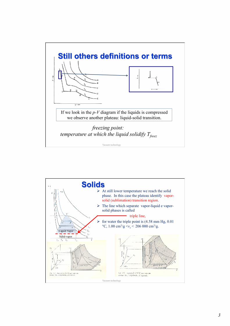
Still others definitions or terms

Vacuum technology

If we look in the p-V diagram if the liquids is compressed we observe another plateau: liquid-solid transition.

freezing point: temperature at which the liquid solidify Tfreez

Solids

Vacuum technology

Ø  At still lower temperature we reach the solid phase. In this case the plateau identify vapor-solid (sublimation) transition region.

Ø  The line which separate vapor-liquid e vapor-solid phases is called

triple line, Ø  for water the triple point is (4.58 mm Hg, 0.01

°C, 1.00 cm3/g <vs < 206 000 cm3/g.

Solid-vapor

Liquid-Vapor

4

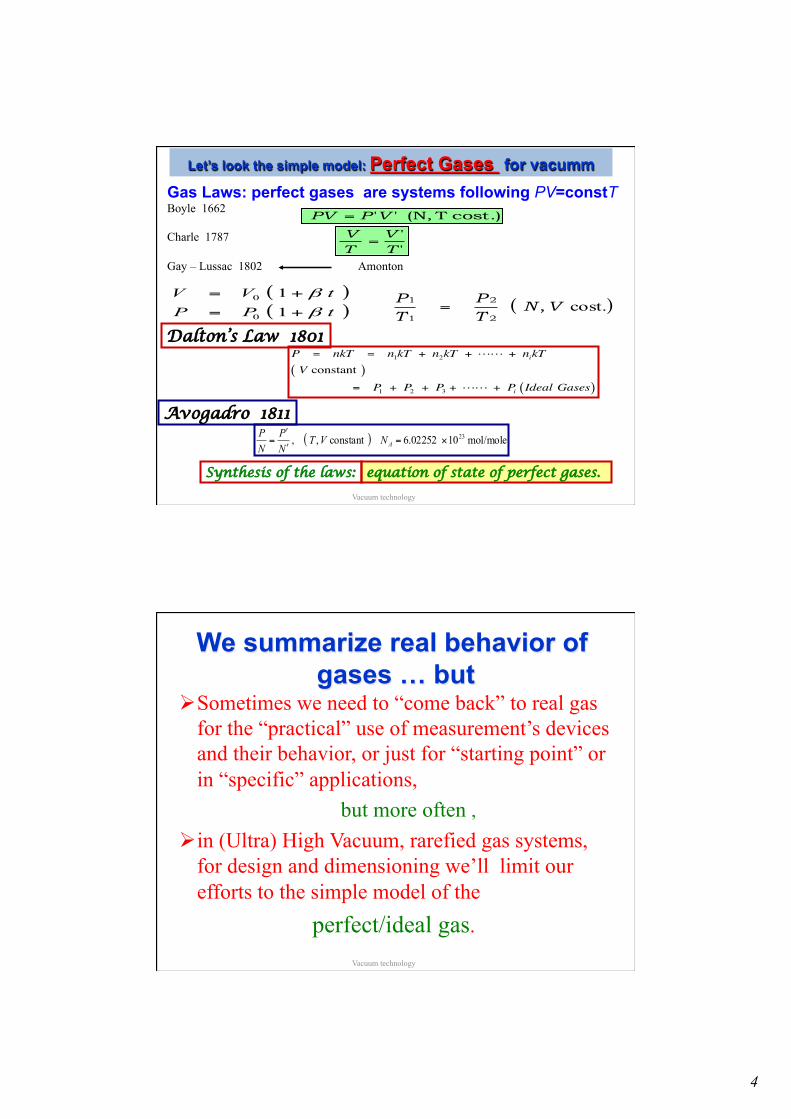
Let’s look the simple model: Perfect Gases for vacumm

Vacuum technology

Gas Laws: perfect gases are systems following PV=constT Boyle 1662

Charle 1787 Gay – Lussac 1802 Amonton

cost.) T(N, '' VPPV =

''

TV

TV

=

( )( )tPP

tVVββ

+=

+=

11

0

0( )cost.VN

TP

TP

,2

2

1

1=

P = nkT = n1kT + n2kT + !! + nikTV constant( )

= P1 + P2 + P3 + !! + Pi Ideal Gases( )

Dalton’s Law 1801

Avogadro 1811 ( ) mol/mole 1002252.6constant ,, 23×=

ʹ

ʹ= ANVTNP

NP

Synthesis of the laws: equation of state of perfect gases.

Ø Sometimes we need to “come back” to real gas for the “practical” use of measurement’s devices and their behavior, or just for “starting point” or in “specific” applications,

but more often , Ø in (Ultra) High Vacuum, rarefied gas systems,

for design and dimensioning we’ll limit our efforts to the simple model of the

perfect/ideal gas.

We summarize real behavior of gases … but

Vacuum technology

5

Vacuum technology

Perfect Gases– Rarified gases P [Torr], V = 22.415 l, T = 273.16 K ,

ν = # moles ⇒

R0 = 62.364 Torr lK mole

≈ 2 cal K−1 mole−1

: gas theof Mass W

molec/mole 106.023 23 ⋅=AN

n = WM

NA

V = molecular density = NA

R0

PT

P (Torr) R0 (Torr cm3 /K) n = 9.66 1018 PT!

"#

$

%&

PVT

= νR0

nkTTNRnPA

0 ==

TRMWPV 0)/( =

k = 8.314 107

6.023 1023 = 1.3805 10-16 erg K−1

PVTRMmNG

0

tot)(mass ==

Previous laws are followed by any gas at low P or at high T.

Loschmidtn # :molec/cm 10 2.687 .stand.cond 319=

Vacuum technology

Ø Molecular weight of gas mixture: ᴥ  Dalton’s law provides for partial pressures: P1 , P2, ... Pn, of the gas weights W1 , W2, ... Wn, and molecular weights

M1 , M2, ... Mn ᴥ  If we describe the total pressure as function of the partial pressures

Air in vacuum calculations

(a) 011

TRMWVPPV

n

i i

in

ii ⋅⋅⎟

⎠

⎞⎜⎝

⎛=⋅⎟

⎠

⎞⎜⎝

⎛= ∑∑

==

(b) / 0 TRMWPV ⋅⋅==

⎟⎠

⎞⎜⎝

⎛⎟⎠

⎞⎜⎝

⎛=

∑∑

=

=n

i i

i

n

ii

MW

WM

1

1

The two equations have to be equal (b)=(a), then we have:

ᴥ  We can provide the average molecular weight as:

6

velocity distribution of gas and mixture of gases kTmv

v evkTmf

dvdn

n2/2

2/3

2/1

2

241 −⎟

⎠

⎞⎜⎝

⎛==π

)(Tffv =

)(mffv =

Most probable velocity:

mkTv

dvdf

pv 2 0 =⇒==

Average velocity (flow): 1.128 22

0

0pave

v

v

ave vmkTv

dvf

dvfvv =⎟

⎠

⎞⎜⎝

⎛=≡

⋅

⋅⋅

=

∫

∫∞+

+∞

π

Root mean square velocity (energy Ekin ):

1.225 3

0

0

2

2p

v

v

rms vmkT

dvf

dvfvvv ==

⋅

⋅⋅

==

∫

∫∞+

+∞

Solution of integral M. Born Atomic physics (DOVER). dvevI vk ∫

∞−⋅=

0

2λκ

Distribution of velocity

7

Vacuum technology

Energy distribution ( ) eTk

kTE

E

Ef

dEdn

n/

2/3

21 −==

π

Average Energy: kTdEf

dEfEE

E

E

ave 23

0

0 =

⋅

⋅⋅

=

∫

∫∞+

+∞

Most probable energy : kTEEfE

21

0 p =≡=∂

∂

Vacuum technology

We will use Pressure (units )

1 Pa = 1 10-5 bar (1 10-2 mbar)

1 atm = 760 Torr (mm Hg)

1 atm = 1.013 bar = 1 013 mbar

1 mbar = 0.75 Torr

Dyne/cm2 = µbar (CGS) named microbar

Newton/m2 = Pa (SI) named Pascal In vacuum technology other units are frequently used mbar and bar deduced from µbar.

8

Ø Vacuum technology is built on the kinetic theory of gases, from which we deduce the following physical quantities:

ᴥ Mean free path ᴥ  Impingement rate

ᴥ Time of monolayer formation

This are useful for vacuum regime definition and

requirement estimations

Vacuum technologies quantities

Vacuum technology

Vacuum technology

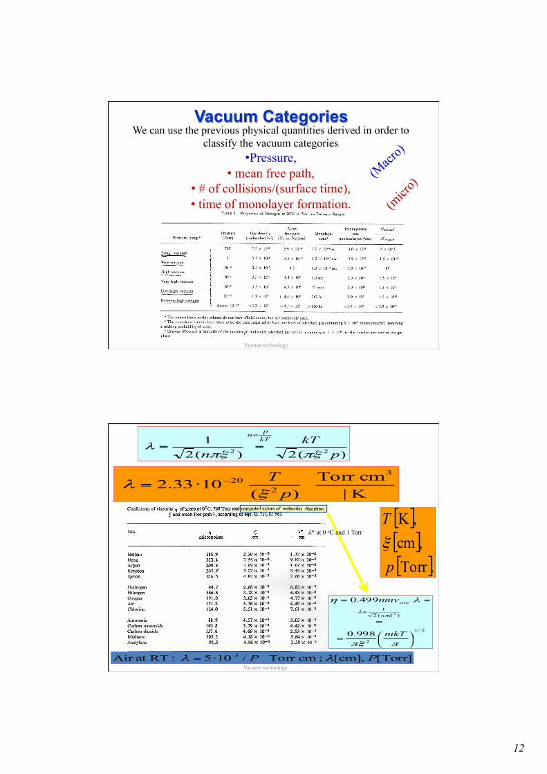
Mean free path λ

Approx calculation : rigid spheres of diameter ξ ~ 10-8 cm

One molecole at v⇒ travel l = vt.it collides any one at 2ξ

( ) nvtnV ⋅⋅=≡⋅2

collisions of # )( swept) ( πξ21/)collisions #/( πξλ nvt ==

)(2

)(21

22 pkT

n

kTpn

πξπξλ

=

==

[Torr] [cm], ;cmTorr /105 :RTat Air -3 PP λλ ⋅=

λ= traveled space / # collisions

Considering the relative velocity:

[mbar] [cm], ;cmmbar /106.6 :RTat Air -3 PP λλ ⋅=

9

Vacuum technology

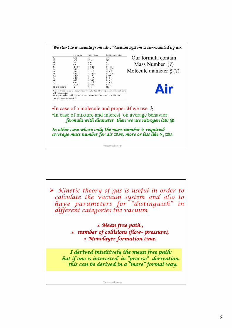
Air • In case of a molecule and proper M we use ξ. • In case of mixture and interest on average behavior:

formula with diameter then we use nitrogen (28) (ξ)

In other case where only the mass number is required: average mass number for air 28.98, more or less like N2 (28).

We start to evacuate from air . Vacuum system is surrounded by air.

Our formula contain Mass Number (?)

Molecule diameter ξ (?).

Vacuum technology

Ø  Kinetic theory of gas is useful in order to calculate the vacuum system and also to have parameters for “distinguish” in different categories the vacuum

ᴥ  Mean free path ,

ᴥ  number of collisions (flow– pressure), ᴥ  Monolayer formation time.

I derived intuitively the mean free path: but if one is interested in “precise” derivation.

this can be derived in a “more” formal way.

10

Vacuum technology

λ precise

dtvdvgfgndVvdvfndW kkkkkk!!!!! )()()( σ==

).( in mol. with collides mol.(

: molecule theofdirection and allover

ids/vdtdtkiPW

kv

==

∫

effkkki

k Lnvdvfvg

gLnW σσ == ∫!!!

)()(… … … … No solution in closed form: Numerical solution allows us to derive λ

)(1033.71

(appross.) 4761.1

1

4 cmPT

n

n

σπσ

σλ

−⋅=≈

≈=

⎥⎦⎤

⎢⎣⎡ oA [Torr], [Torr], σPT

Assuming nk constant along s (tot= L)

)(2

1 2πξ

λn

≈

vi in vk, , nk and f(vk) . Reference system on the k molecule: i molecule moves with vi

relative velocity g=vi-vk. dV = σgdt.

H. Pauly Atom, Molecule and Cluster Beams I Springer-Verlag Berlin 2000

Vacuum technology

# of collisions (flow, pressure) formal derivation from Maxwell distribution.

# particles impinging on dA in dt from dω (θ e φ). dvvfdn )(

4πω

⇒= dAdtvdV θcos

∫ ∫ ∫∞

==ππ

ϕθθθπ

2

0

2/

0 0 4 sincos)(

4 collision # vnddvdvvfn

tA

∫ ∫ ∫∞

==ππ

ϕθθθπ

2

0

2/

0 0

222

3 sincos)(

2dtdAvnmdtdAddvfvnmFdt

2

31 vnmP =

# collisions /dA in dt.

Pressure (momentum transfer normal to the surface: dp=2mvcosθ)

nkTP =

,3 FrommkTvrms =

dV)(4

dvvfdnπω

:23or kTEave =

# collisioni /(unit of A and t)

unit olumeparticle/v #

11

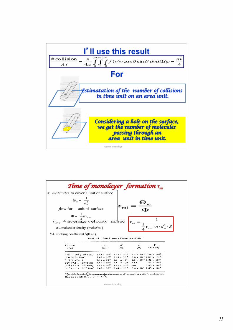
I’ll use this result

Vacuum technology

∫ ∫ ∫∞

==ππ

ϕθθθπ

2

0

2/

0 0 4 sincos)(

4 collision # vnddvdvvfn

tA

Estimatation of the number of collisions in time unit on an area unit.

Considering a hole on the surface, we get the number of molecules

passing through an area unit in time unit.

For

Vacuum technology

Time of monolayer formation τml

m/sec velocity average =!avev

)(molec/mdensity molecular 3=!n

# molecules to cover a unit of surface

Θm = 1dm

2

flow for unit of surface

Φ= 14nvave

⎫

⎬

⎪⎪⎪⎪

⎭

⎪⎪⎪⎪

S != sticking coefficient S(0÷1).

Φ

Θ= m

mlτ

Sdnv mave

ml

⋅⋅⋅=

2

41

1τ

12

Vacuum technology

Vacuum Categories We can use the previous physical quantities derived in order to

classify the vacuum categories • Pressure,

•  mean free path, •  # of collisions/(surface time), •  time of monolayer formation.

Vacuum technology

)(2

)(21

22 pkT

n

kTpn

πξπξλ

=

==

[Torr] [cm], ; cmTorr /105 :RTat Air -3 PP λλ ⋅=

[ ][ ][ ].Torr

,cm ,K

p

Tξ

K|cmTorr

)( 1033.2

3

220

pTξ

λ −⋅=

2/1

2

)(21

998.0

499.0

2

⎟⎠

⎞⎜⎝

⎛=

=

==

=

ππξ

λη

πξλ

mkT

nmv

n

ave

λ* at 0 oC and 1 Torr

13

Vacuum technology

Transport phenomena: Viscosity

Viscosity coefficient (η), from KTG is derived from the momentum transfer between different layer of the gas:

FxAxz

= −η duxdy

Tangential force

λνη mn31

= n: molecular density m: molecule mass. ν : velocity λ : mean free path.

( ) ( )20

2/1

20

2/3

2/14499.0499.0

ddmn

TmTkm∝==

πλνη

31 2/1

3⇒=

=

=σλ

λνηn

mkTvav

mn Indipendent from n (at given T) and then from P

Berkeley Physics – Statistical Physics.

σνη

nmn

21

31

=

Ø Transport phenomena are useful in vacuum technology for its ᴥ Transition regime to reach the high vacuum ᴥ  In some gauges, for pressure measurements ᴥ  In some pumping systems, which use the

properties of gases, condensation (cryos).

We’ll consider this properties from the practical point of view.

But … still we have to consider real gas properties

Vacuum technology

14

Vacuum technology

Transport phenomena: thermal conductivity

λνvcmnk31

=

tyconductivi thermal flowheat

- dydTkQ =

Heat is the transmission of energy, therefore in the previous scheme we consider the transfer of energy (kinetic energy)

Practical use in vacuum gauge: Thermo-cross and Pirani

Vck ⋅=η

( ) νηγ ck 5941

−=

We can use what was derived for η:

The previous approssimated equation, in a more precise form (γ =cp /cv):

( )20

2/1

dk

Tm∝∝η

Then we derive same behavior like for η also for k

Berkeley Physics – Statistical Physics.

Vacuum technology

Transport phenomena: diffusion

λvD31

=

( )mkT

pD

n

mkTvav

32/1

3

161

σ

σλ

≈==

=

23given a @given a @ 1 T

pD

P T

∝∝

dxdnD

dxdnD 2

21

1 , −=Γ−=Γ

Diffusion of one kind of molecules from KTG in case of one kind molecule (self-diffusion) :

Diffusion law for two different gas at different molecular density gradient.

1,22,1 Flow=Γ tcoefficiendiffusion =D

15

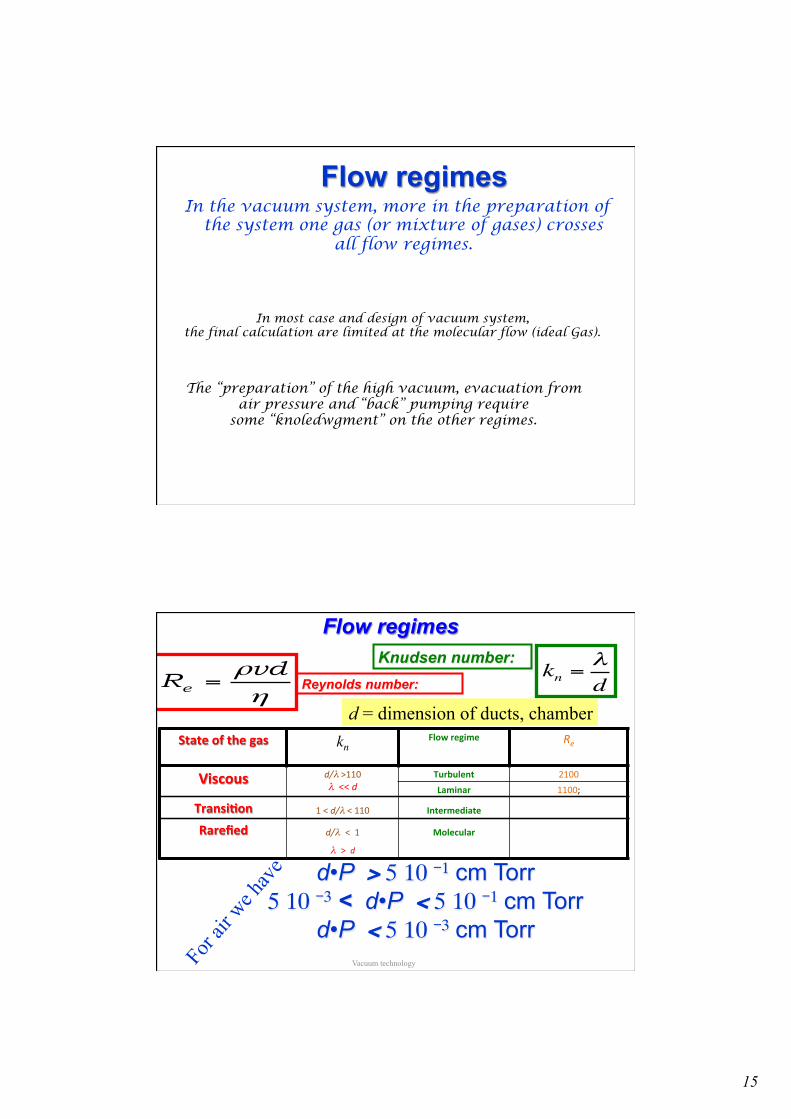
In the vacuum system, more in the preparation of the system one gas (or mixture of gases) crosses

all flow regimes.

Flow regimes

In most case and design of vacuum system, the final calculation are limited at the molecular flow (ideal Gas).

The “preparation” of the high vacuum, evacuation from air pressure and “back” pumping require

some “knoledwgment” on the other regimes.

Vacuum technology

Flow regimes Knudsen number:

kn =λdReynolds number:

ηρvd

Re =

d•P > 5 10 -1 cm Torr5 10 -3 < d•P < 5 10 -1 cm Torr

d•P < 5 10 -3 cm Torr

Stateofthegas kn Flowregime Re

Viscous d/λ>110λ<<d

Turbulent 2100Laminar 1100;

Transi8on 1<d/λ<110 Intermediate

Rarefied d/λ <1

λ >d

Molecular

d = dimension of ducts, chamber

16

Thro

ughp

ut/d

Vacuum technology

In the region

“molecular flow” Or

“molecular regime”, calculation and design

come out from the KTG.

For HV and UHV, We can limit the

discussion Here.

Ø We’ll introduce some useful physical M-scopic quantities.

Ø Then we’ll provide “model” to understand them and “tools” for calculation

via the µ-scopic approach of the

KTG.

Vacuum-gas physical quantities

Vacuum technology

17

Vacuum technology

Throughput Q Q =

d(PV )dt

; SI Pa m3

s!

"#

$

%&=WattThroughput Q:

dtdNkT

dtPVdQ

NkTPVT

==

=

=cost)(

:

Q =d(PV )dt

= ddt

WMR0T

!

"#

$

%& =T=cost

=T= cost R0T

MdWdt

;

TRQ

TkNQmoleskgN

00

)sec/( ==−ʹ

TRMQ

TkNQMkgm

00

)sec/(' ==

{Relation between Throughput & Φmol

{Relation between Throughput & Φmass

Molar flow or mass flow it’s correlated directly to the Q at T fixed.

Vacuum technology

P1 P2

IF ΔP > 0 ; we expected a total gas flow (Q) Dominant from the side at higher density :

s

m 3

⎥⎦

⎤⎢⎣

⎡

Δ=PQC

21 PP >

Q→

We define conductance ( C ):

Equivalent in electricity VICΔ

=

Conductance (Macro definition)

18

Vacuum technology

Pumping Speed

⎥⎦

⎤⎢⎣

⎡=

sm3

dtdVS

ii PQS =

CSS111

21

+=

P1

P2 C

We define pumping speed ( S ):

S is the volume of gas evacuated in t at a given P

Stationary condition (p = cost) : Q = P d(V )dt

;S Q is the physical quantity conserved in a vacuum system

(at T constant along the system).

Q

Then from the definition it follows the master equations:

more confortable l/s.

Vacuum technology

Conductances in parallel and in serie

!+++= 321 CCCC

321

1111CCCC

++=

We can derive how to sum different conductance from the electric equivalent:

If we have conductance in parallel it follows:

VICΔ

=

If we have conductance in serie it follows:

continua

19

Thanks to the Kinetics Theory of Gas calculations for vacuum systems (molecular regime)

are more simple than in the case of “real gas” (viscous regime),

Then also the

design of systems

the µ –scopic approach is useful for calculation in the

molecular regime (randomized molecules).

Calculation of Vacuum physical quantities

Vacuum technology

Vacuum technology

Derivation of C - (µ-scopic) molecular flow

A1 A2

11

1111

nSnvAN

=

==!

22

2222

S nnvAN

=

==!

21 NNN pt!!! ==∀Stationary condition

)( 21 nnnN −=Δ∝!

Effective flow torwards less molecular density:

)( 21 nn

NCdef

−= !

)/1()/1(/1 21 SSC −=As a result we derive:

m3

s!"#

$%&

20

Vacuum technology

C in parallel or in serie (µ-scopic) a

b

1 2 C in parallel

⎭⎬⎫

−=

−=

)()(

21

21

nnCNnnCN

bb

aa

!!

)( 21|| nnCNNN ba −==+ !!! !++= ba CCC||

)()()( 313221 nnCnnCnnCN sba −=−=−=!

!++= bas CCC /1/1/1a b

1 2 3 ╚╬╬╬╬╬╬╬╬╬╬╬╬╬╬╬╬╬╬╬╬╝

C in serie

Vacuum technology

From the µ-scopic to M-scopic # molecole / t =

)(

)(

)(

21

21

21

PPCQSP

kTnkTnCkTN

nnCNnN

nkTP

SnN

nkTP

SnN

kT

kT

−==≡

≡−=≡

≡−=≡Δ∝

=

=

=

=

⋅

⋅

!

!!

!!

N!

How to connect it to Q [Pa m3/s=W]

more “confortable” units for Q are mbar l/s

21

Vacuum technology

n Vacuum

A

[ ]/seccm )/(1064.3 3213 AMTq/ndV/dt ⋅==

)()/(1064.3 21213

21 PPAMTQQQ −⋅=−=

l/s )/(64.3/ 21AMTPQC ⋅=Δ=

P1 P2

A

Conductance of an aperture

Q(1,2) = P(1,2)dV / dt = 3.64 ⋅103(T /M )1

2AP(1,2) µbar cm3 /sec

avenv41 =φ

How many molecules travel through A in a time t? [ ]mol/sec )/(1064.3 2

13 nAMTAq ⋅==φVolume of gas passing through A?

µ-sco

pic

Μ-sc

opic

←→ ←→ ←→ ←→

C indipendent from P

CA = 2.86 ⋅ TM( ) ⋅D2 l

s"#

$%; D = [cm] Circular aperture Α=πD2/4