6_Introduction to Hypothesis Testing_2012

I. Estimation continued… • Least Squares (OLS)

• Likelihood

II. Hypothesis Testing • t-test

one sample

two sample

paired

• non-parametric tests assumptions

Mann-Whitney-Wilcoxon

Frequentist (classical approaches)

• when sampling distribution is known

– Ordinary Least Squares

– Maximum Likelihood

• when sampling distribution is unknown

– Numerical Resampling

• Bootstrap

• Jackknife

• Permutation / Randomization tests

Bayesian inference - estimation

Methods for estimating parameters

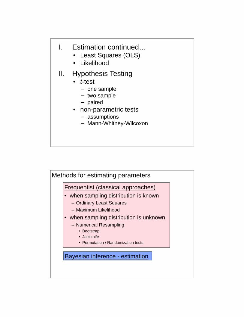
Ordinary Least Squares (OLS)

• the parameter estimate that minimizes the sum of

squared differences between each value in a

sample and the parameter

in this example, the parameter is the mean

OLS =min yi y ( )i=1

n 2

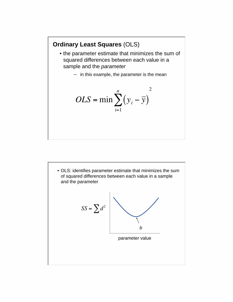
SS = d2

b

• OLS: identifies parameter estimate that minimizes the sum

of squared differences between each value in a sample

and the parameter

parameter value

Ordinary Least Squares (OLS)

• frequently used to estimate parameters of linear models (e.g., linear regression, y=a+bx)

• unbiased and has minimum variance when distributional assumptions are met (i.e., is a precise estimator)

• no distributional assumptions required for point estimates

• for interval estimation & hypothesis testing, OLS estimators have restrictive assumptions of normality and patterns of variance

Maximum Likelihood (ML)

• estimate of a parameter that maximizes the

likelihood function based on the observed data

likelihood function estimates likelihood of observing sample data for all possible values of the parameter

• e.g., likelihood of observing the data for all possible values of

the mean, , in a normally distributed population

when assumptions of specified underlying distribution

are met, ML estimators are unbiased and have

minimum variance

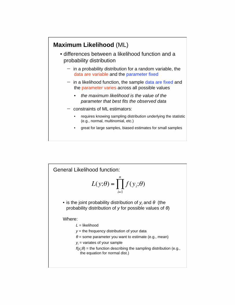
Maximum Likelihood (ML)

• differences between a likelihood function and a

probability distribution

in a probability distribution for a random variable, the data are variable and the parameter fixed

in a likelihood function, the sample data are fixed and

the parameter varies across all possible values

• the maximum likelihood is the value of the

parameter that best fits the observed data

constraints of ML estimators:

• requires knowing sampling distribution underlying the statistic

(e.g., normal, multinomial, etc.)

• great for large samples, biased estimates for small samples

General Likelihood function:

L(y; ) = f (yi; )i=1

n

• is the joint probability distribution of yi and (the

probability distribution of y for possible values of )

Where:

L = likelihood

y = the frequency distribution of your data

= some parameter you want to estimate (e.g., mean)

yi = variates of your sample

f(yi; ) = the function describing the sampling distribution (e.g.,

the equation for normal dist.)

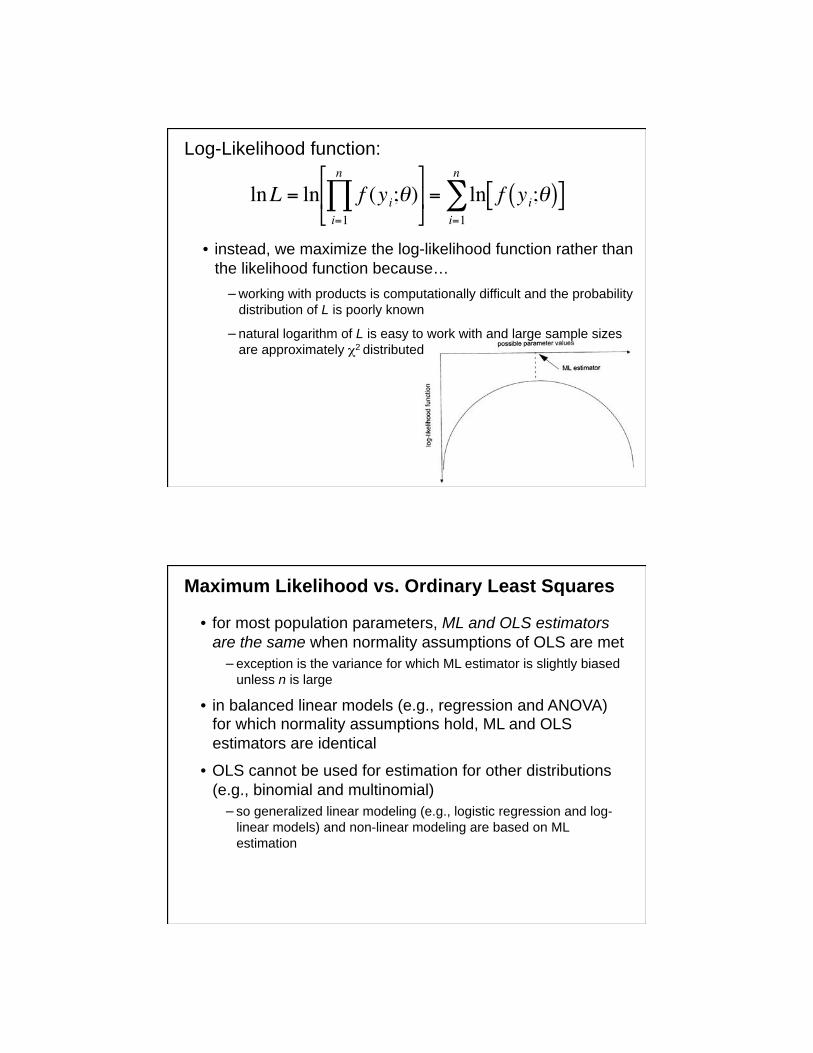
Log-Likelihood function:

• instead, we maximize the log-likelihood function rather than

the likelihood function because…

working with products is computationally difficult and the probability

distribution of L is poorly known

natural logarithm of L is easy to work with and large sample sizes

are approximately 2 distributed

lnL = ln f (yi; )i=1

n

= ln f yi;( )[ ]

i=1

n

Maximum Likelihood vs. Ordinary Least Squares

• for most population parameters, ML and OLS estimators

are the same when normality assumptions of OLS are met

exception is the variance for which ML estimator is slightly biased

unless n is large

• in balanced linear models (e.g., regression and ANOVA) for which normality assumptions hold, ML and OLS

estimators are identical

• OLS cannot be used for estimation for other distributions

(e.g., binomial and multinomial)

so generalized linear modeling (e.g., logistic regression and log-

linear models) and non-linear modeling are based on ML

estimation

Introduction to hypothesis testing

• main approach to statistical inference in biology

So far covered:

• collecting data samples

• estimating parameters from sample statistics

• calculated SE and CI as estimators of reliability

of these statistics

Now, we want…

some objective way to decide whether our sample

differs from some expected distribution, or from other similarly collected samples

Hypothesis testing

Classical statistical hypothesis testing rests on disproving H0:

• must state a statistical null hypothesis (Ho)

includes all possibilities except the prediction of research hypothesis, HA

H0 is usually a hypothesis of no difference or effect

because…

(1) inductive reasoning requires verification of all possible

observations (impossible) and…

(2) we often don’t know what constitutes proof of a hypothesis

(alternative biological hypotheses are often more vague than

H0)

in contrast, we know what constitutes disproof (falsification),

because null hypotheses are exact

disproof of H0 constitutes evidence for HA

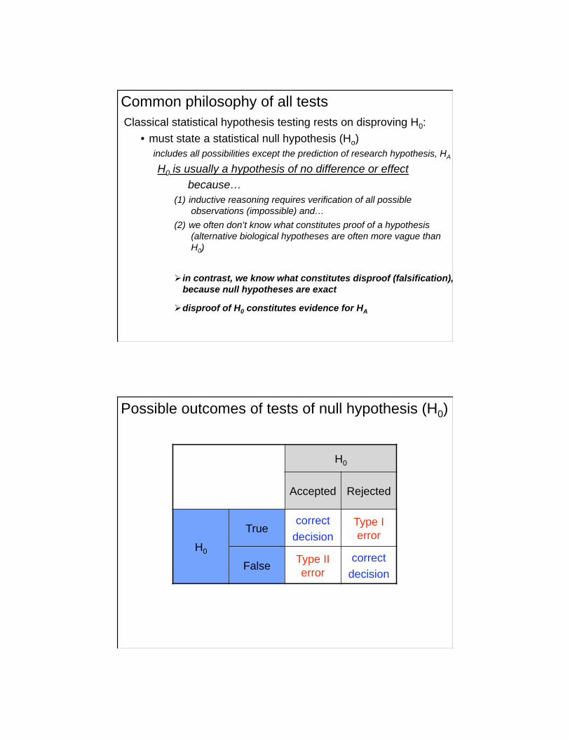
Common philosophy of all tests

H0

Accepted Rejected

H0

True correct

decision

Type I

error

False Type II

error

correct

decision

Possible outcomes of tests of null hypothesis (H0)

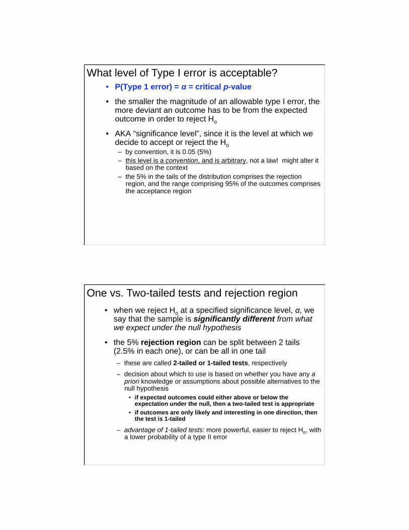
• P(Type 1 error) = = critical p-value

• the smaller the magnitude of an allowable type I error, the more deviant an outcome has to be from the expected outcome in order to reject Ho

• AKA “significance level”, since it is the level at which we decide to accept or reject the Ho – by convention, it is 0.05 (5%)

– this level is a convention, and is arbitrary, not a law! might alter it based on the context

– the 5% in the tails of the distribution comprises the rejection region, and the range comprising 95% of the outcomes comprises the acceptance region

What level of Type I error is acceptable?

• when we reject Ho at a specified significance level, , we say that the sample is significantly different from what we expect under the null hypothesis

• the 5% rejection region can be split between 2 tails (2.5% in each one), or can be all in one tail

– these are called 2-tailed or 1-tailed tests, respectively

– decision about which to use is based on whether you have any a priori knowledge or assumptions about possible alternatives to the null hypothesis

• if expected outcomes could either above or below the expectation under the null, then a two-tailed test is appropriate

• if outcomes are only likely and interesting in one direction, then the test is 1-tailed

– advantage of 1-tailed tests: more powerful, easier to reject Ho, with a lower probability of a type II error

One vs. Two-tailed tests and rejection region

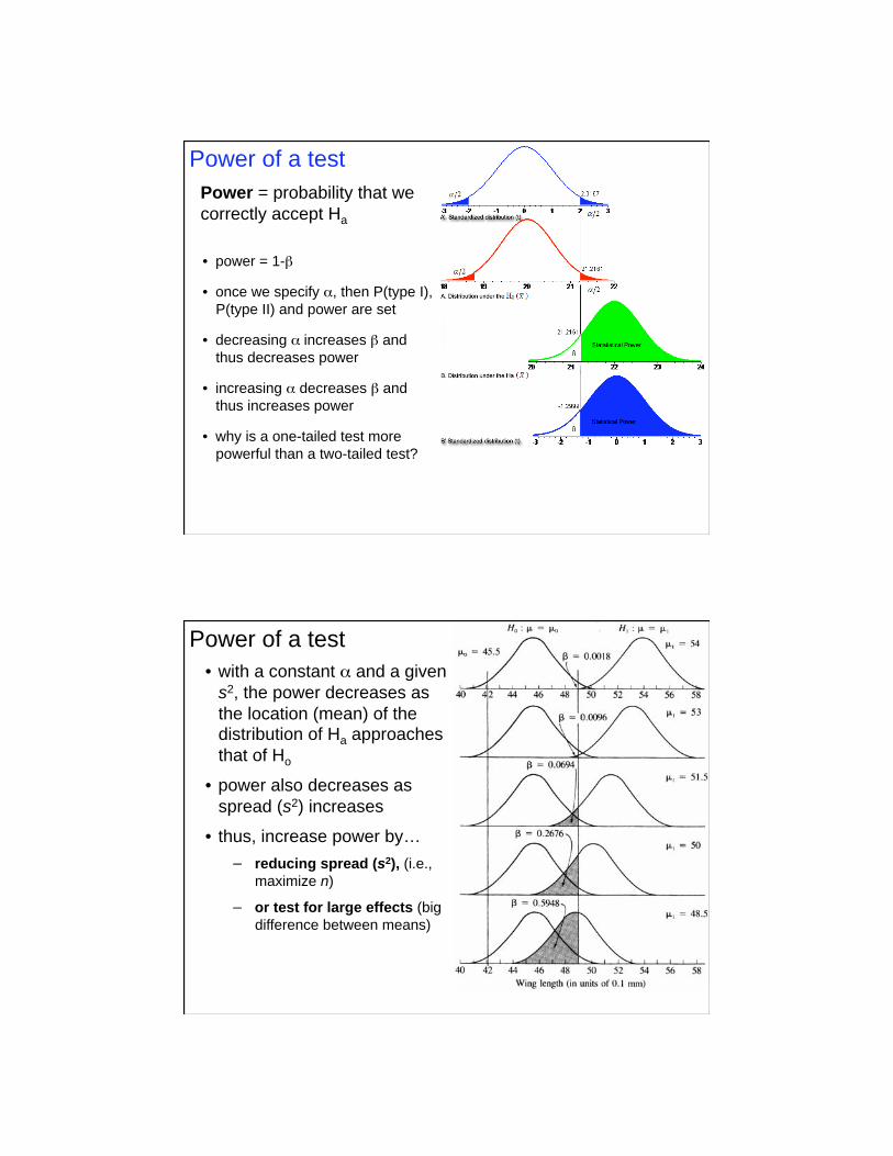
• power = 1-

• once we specify , then P(type I),

P(type II) and power are set

• decreasing increases and

thus decreases power

• increasing decreases and

thus increases power

• why is a one-tailed test more

powerful than a two-tailed test?

Power = probability that we

correctly accept Ha

Power of a test

• with a constant and a given

s2, the power decreases as

the location (mean) of the distribution of Ha approaches

that of Ho

• power also decreases as

spread (s2) increases

• thus, increase power by…

reducing spread (s2), (i.e.,

maximize n)

or test for large effects (big

difference between means)

Power of a test

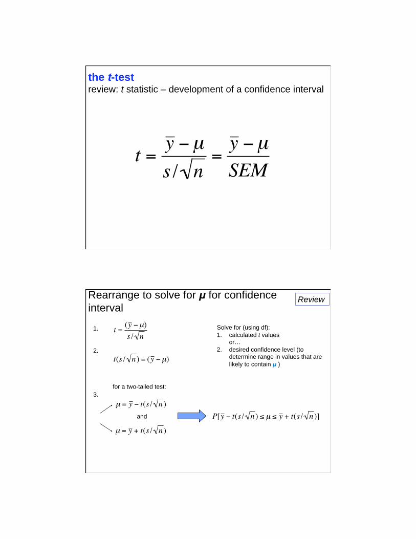
the t-test review: t statistic – development of a confidence interval

t =y μ

s / n=

y μ

SEM

Rearrange to solve for μ for confidence

interval

and

1.

2.

3.

for a two-tailed test:

Solve for (using df):

1. calculated t values or…

2. desired confidence level (to determine range in values that are

likely to contain μ ) t(s / n ) = (y μ)

t =(y μ)

s / n

μ = y t(s / n )

μ = y + t(s / n )

P[y t(s / n ) μ y + t(s / n )]

Review

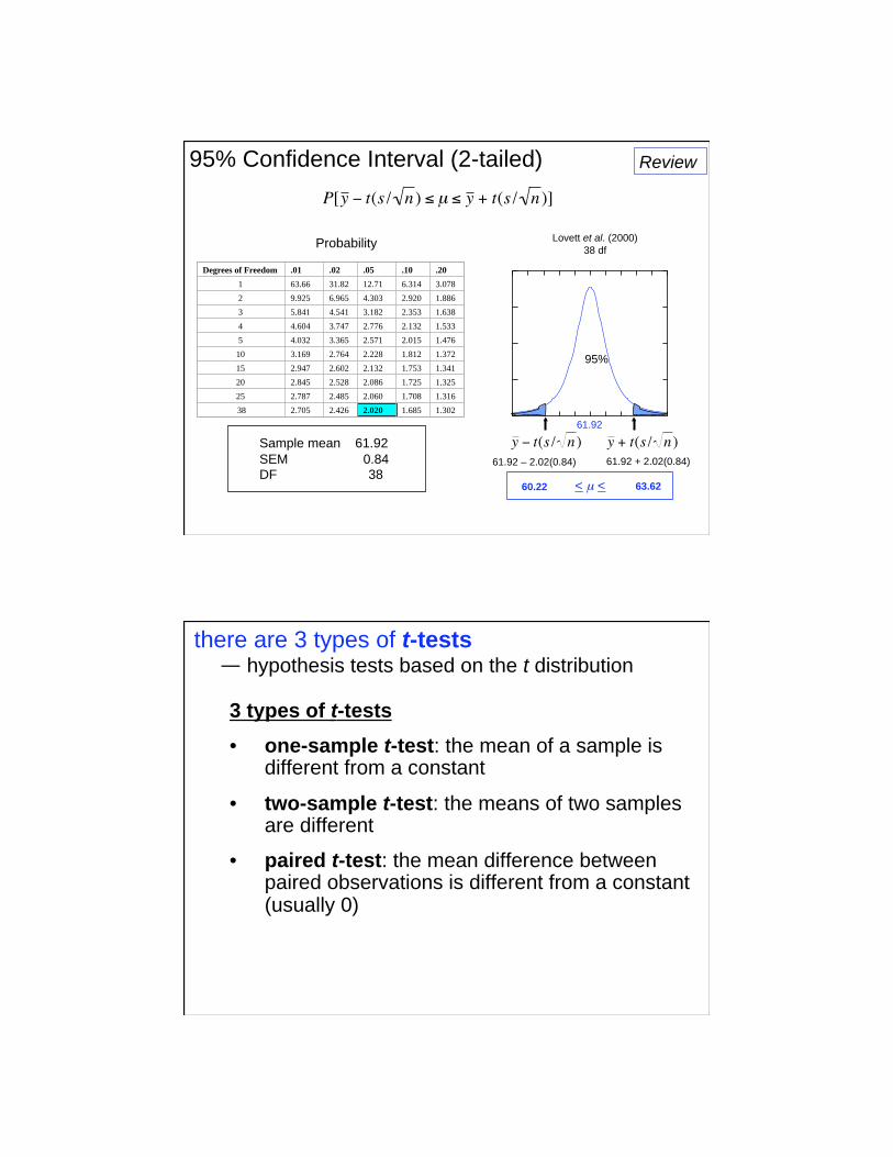
Degrees of Freedom .01 .02 .05 .10 .20

1 63.66 31.82 12.71 6.314 3.078

2 9.925 6.965 4.303 2.920 1.886

3 5.841 4.541 3.182 2.353 1.638

4 4.604 3.747 2.776 2.132 1.533

5 4.032 3.365 2.571 2.015 1.476

10 3.169 2.764 2.228 1.812 1.372

15 2.947 2.602 2.132 1.753 1.341

20 2.845 2.528 2.086 1.725 1.325

25 2.787 2.485 2.060 1.708 1.316

38 2.705 2.426 2.020 1.685 1.302

Probability

61.92

95%

Lovett et al. (2000)

38 df

61.92 – 2.02(0.84)

60.22

61.92 + 2.02(0.84)

63.62 < μ <

Sample mean 61.92

SEM 0.84 DF 38

P[y t(s / n ) μ y + t(s / n )]

y t(s / n ) y + t(s / n )

95% Confidence Interval (2-tailed) Review

3 types of t-tests

• one-sample t-test: the mean of a sample is different from a constant

• two-sample t-test: the means of two samples are different

• paired t-test: the mean difference between paired observations is different from a constant (usually 0)

there are 3 types of t-tests — hypothesis tests based on the t distribution

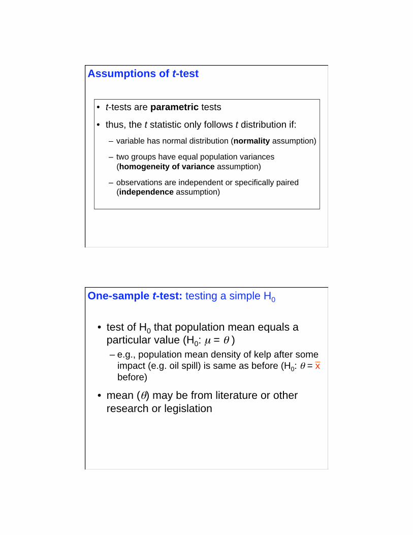
• t-tests are parametric tests

• thus, the t statistic only follows t distribution if:

– variable has normal distribution (normality assumption)

– two groups have equal population variances

(homogeneity of variance assumption)

– observations are independent or specifically paired (independence assumption)

Assumptions of t-test

• test of H0 that population mean equals a

particular value (H0: μ = )

– e.g., population mean density of kelp after some

impact (e.g. oil spill) is same as before (H0: = x

before)

• mean ( ) may be from literature or other

research or legislation

One-sample t-test: testing a simple H0

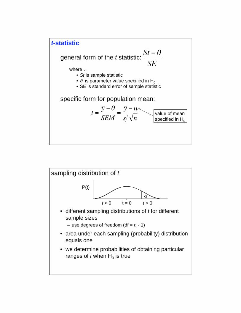
general form of the t statistic:

where…

• St is sample statistic

• is parameter value specified in H0 • SE is standard error of sample statistic

value of mean

specified in H0

St

SE

t =y

SEM=

y μ

s n

t-statistic

specific form for population mean:

• different sampling distributions of t for different

sample sizes

– use degrees of freedom (df = n - 1)

• area under each sampling (probability) distribution

equals one

• we determine probabilities of obtaining particular

ranges of t when H0 is true

sampling distribution of t

P(t)

t = 0 t > 0 t < 0

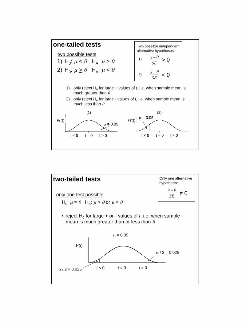
1) only reject H0 for large + values of t, i.e. when sample mean is

much greater than

2) only reject H0 for large - values of t, i.e. when sample mean is

much less than

Two possible independent

alternative hypotheses:

1) H0: μ < HA: μ >

2) H0: μ > HA: μ <

(1) (2)

one-tailed tests

two possible tests > 0

< 0

1)

2)

y

SE

y

SE

H0: μ = HA: μ > or μ <

• reject H0 for large + or - values of t, i.e. when sample

mean is much greater than or less than

P(t)

t = 0 t > 0 t < 0 / 2 = 0.025

/ 2 = 0.025

= 0.05

0

Only one alternative

hypothesis: two-tailed tests

only one test possible y

SE

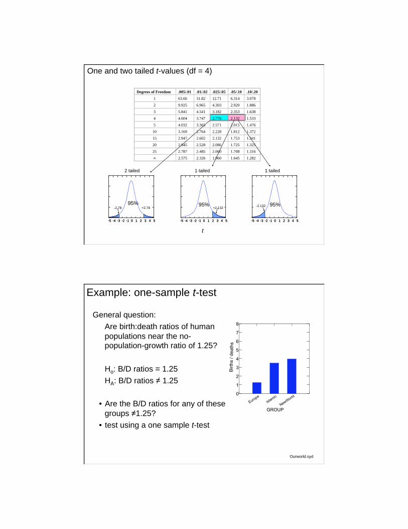
Degrees of Freedom .005/.01 .01/.02 .025/.05 .05/.10 .10/.20

1 63.66 31.82 12.71 6.314 3.078

2 9.925 6.965 4.303 2.920 1.886

3 5.841 4.541 3.182 2.353 1.638

4 4.604 3.747 2.776 2.132 1.533

5 4.032 3.365 2.571 2.015 1.476

10 3.169 2.764 2.228 1.812 1.372

15 2.947 2.602 2.132 1.753 1.341

20 2.845 2.528 2.086 1.725 1.325

25 2.787 2.485 2.060 1.708 1.316

2.575 2.326 1.960 1.645 1.282

-5 -4 -3 -2 -1 0 1 2 3 4 5 -5 -4 -3 -2 -1 0 1 2 3 4 5

-2.78 +2.78

95%

-5 -4 -3 -2 -1 0 1 2 3 4 5 -5 -4 -3 -2 -1 0 1 2 3 4 5

+2.132 95%

-5 -4 -3 -2 -1 0 1 2 3 4 5 -5 -4 -3 -2 -1 0 1 2 3 4 5

-2.132 95%

One and two tailed t-values (df = 4)

2 tailed 1 tailed 1 tailed

t

General question:

Are birth:death ratios of human

populations near the no-population-growth ratio of 1.25?

Ho: B/D ratios = 1.25

HA: B/D ratios 1.25

• Are the B/D ratios for any of these

groups 1.25?

• test using a one sample t-test

Ourworld.syd

Example: one-sample t-test

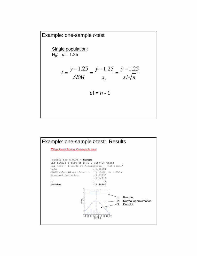
Single population:

H0: μ = 1.25

df = n - 1

Example: one-sample t-test

t =y 1.25

SEM=

y 1.25

sy

=y 1.25

s / n

1. Box plot

2. Normal approximation 3. Dot plot

Hypothesis Testing: One-sample t-test

Results for GROUP$ = Europe

One-sample t-test of B_TO_D with 20 Cases

Ho: Mean = 1.25000 vs Alternative = 'not equal'

Mean : 1.25701

95.00% Confidence Interval : 1.15735 to 1.35668

Standard Deviation : 0.21295

t : 0.14727

df : 19

p-value : 0.88447

Example: one-sample t-test: Results

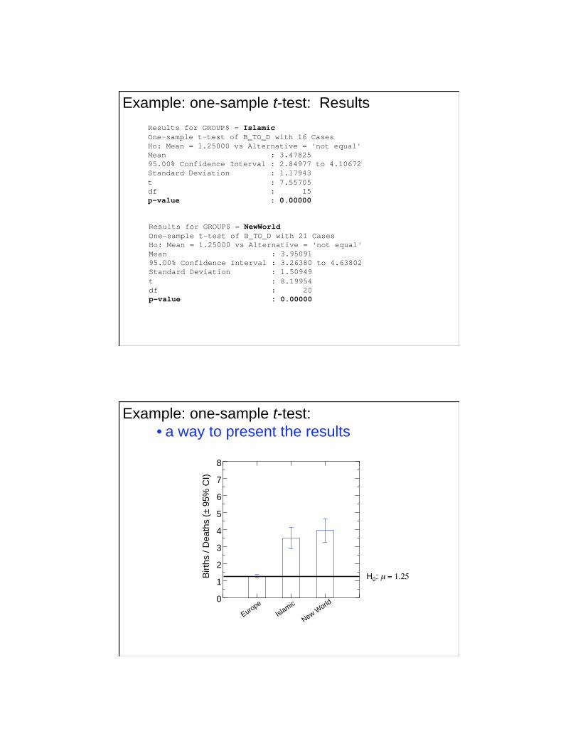
Results for GROUP$ = Islamic



Mean : 3.47825



t : 7.55705

df : 15

p-value : 0.00000

Results for GROUP$ = NewWorld



Mean : 3.95091



t : 8.19954

df : 20

p-value : 0.00000

Example: one-sample t-test: Results

Europe

Islam

ic

New World

0

1

2

3

4

5

6

7

8

Birth

s /

Death

s (

± 9

5%

CI)

H0: μ = 1.25

Example: one-sample t-test:

• a way to present the results

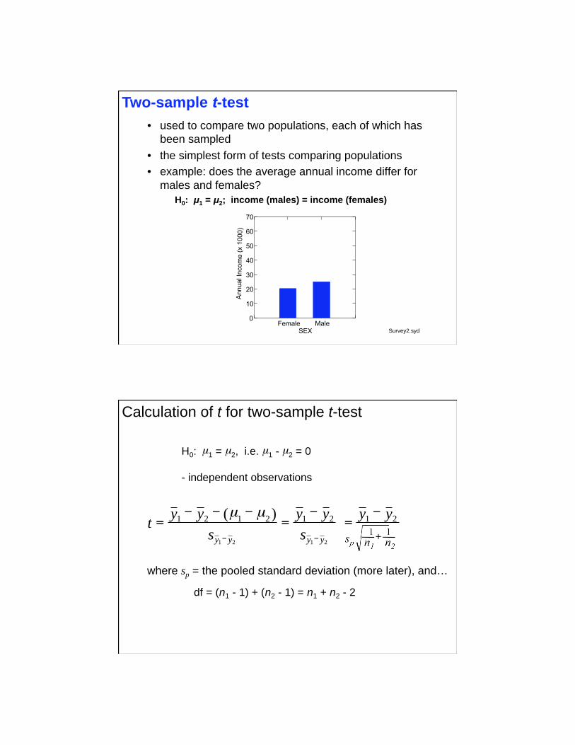
• used to compare two populations, each of which has

been sampled

• the simplest form of tests comparing populations

• example: does the average annual income differ for

males and females?

H0: μ1 = μ2; income (males) = income (females)

Survey2.syd

Two-sample t-test

H 0 : μ 1 = μ

2 , i.e. μ 1 - μ

2 = 0

- independent observations

df = ( n 1 - 1) + ( n 2 - 1) = n 1 + n 2 - 2

2 1 2 1

2 1 2 1 2 1 ) (

y y y y s

y y

s

y y t

=

=

μ μ 2 1 y y

=

where sp = the pooled standard deviation (more later), and…

Calculation of t for two-sample t-test

y1

t =

y2

1

n1

1

n2

+ sp

- 5 - 4 - 3 - 2 - 1 0 1 2 3 4 5 0.0

0.1

0.2

0.3

0.4

Pro

babili

ty o

f t

- 5 - 4 - 3 - 2 - 1 0 1 2 3 4 5 0.0

0.1

0.2

0.3

0.4

6 7 8 9

HA true

- 5 - 4 - 3 - 2 - 1 0 1 2 3 4 5 0.0

0.1

0.2

0.3

0.4

Pro

babili

ty o

f t

- 5 - 4 - 3 - 2 - 1 0 1 2 3 4 5 0.0

0.1

0.2

0.3

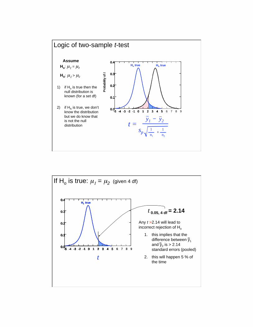
0.4 Ho true Ho: μ1 = μ2

HA: μ1 > μ2

1) if Ho is true then the

null distribution is known (for a set df)

2) if HA is true, we don’t

know the distribution

but we do know that is not the null

distribution

Assume

Logic of two-sample t-test

t

- 5 - 4 - 3 - 2 - 1 0 1 2 3 4 5 0.0

0.1

0.2

0.3

0.4

- 5 - 4 - 3 - 2 - 1 0 1 2 3 4 5 0.0

0.1

0.2

0.3

0.4

6 7 8 9 - 5 - 4 - 3 - 2 - 1 0 1 2 3 4 5 0.0

0.1

0.2

0.3

0.4

- 5 - 4 - 3 - 2 - 1 0 1 2 3 4 5 0.0

0.1

0.2

0.3

0.4 H o true

- 5 - 4 - 3 - 2 - 1 0 1 2 3 4 5 0.0

0.1

0.2

0.3

0.4

- 5 - 4 - 3 - 2 - 1 0 1 2 3 4 5 0.0

0.1

0.2

0.3

0.4

6 7 8 9 - 5 - 4 - 3 - 2 - 1 0 1 2 3 4 5 0.0

0.1

0.2

0.3

0.4

- 5 - 4 - 3 - 2 - 1 0 1 2 3 4 5 0.0

0.1

0.2

0.3

0.4 H o true

t 0.05, 4 df = 2.14

Any t >2.14 will lead to

incorrect rejection of Ho

1. this implies that the

difference between y1

and y2 is > 2.14

standard errors (pooled)

2. this will happen 5 % of

the time

If Ho is true: μ1 = μ2 (given 4 df)

- 5 - 4 - 3 - 2 - 1 0 1 2 3 4 5 0.0

0.1

0.2

0.3

0.4

- 5 - 4 - 3 - 2 - 1 0 1 2 3 4 5 0.0

0.1

0.2

0.3

0.4

6 7 8 9 - 5 - 4 - 3 - 2 - 1 0 1 2 3 4 5 0.0

0.1

0.2

0.3

0.4

- 5 - 4 - 3 - 2 - 1 0 1 2 3 4 5 0.0

0.1

0.2

0.3

0.4

- 5 - 4 - 3 - 2 - 1 0 1 2 3 4 5 0.0

0.1

0.2

0.3

0.4

- 5 - 4 - 3 - 2 - 1 0 1 2 3 4 5 0.0

0.1

0.2

0.3

0.4

6 7 8 9 - 5 - 4 - 3 - 2 - 1 0 1 2 3 4 5 0.0

0.1

0.2

0.3

0.4

- 5 - 4 - 3 - 2 - 1 0 1 2 3 4 5 0.0

0.1

0.2

0.3

0.4 HA true

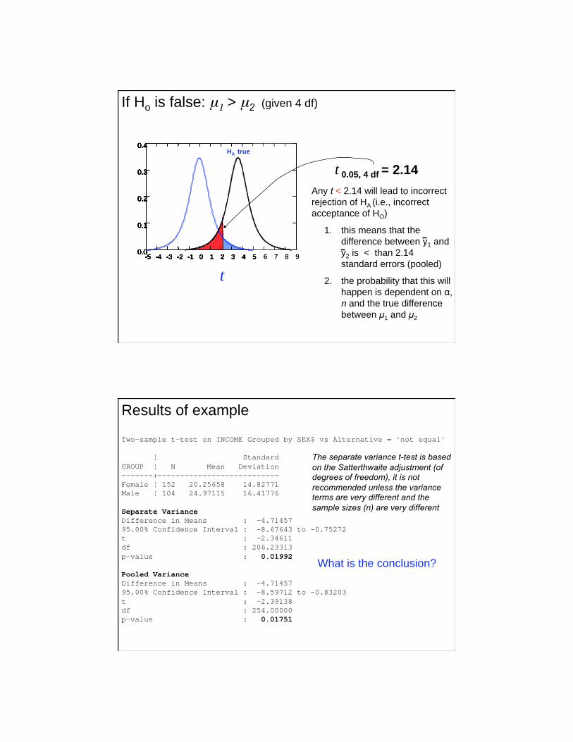
t 0.05, 4 df = 2.14

Any t < 2.14 will lead to incorrect

rejection of HA (i.e., incorrect

acceptance of HO)

1. this means that the

difference between y1 and

y2 is < than 2.14

standard errors (pooled)

2. the probability that this will

happen is dependent on ,

n and the true difference

between μ1 and μ2

If Ho is false: μ1 > μ2 (given 4 df)

t

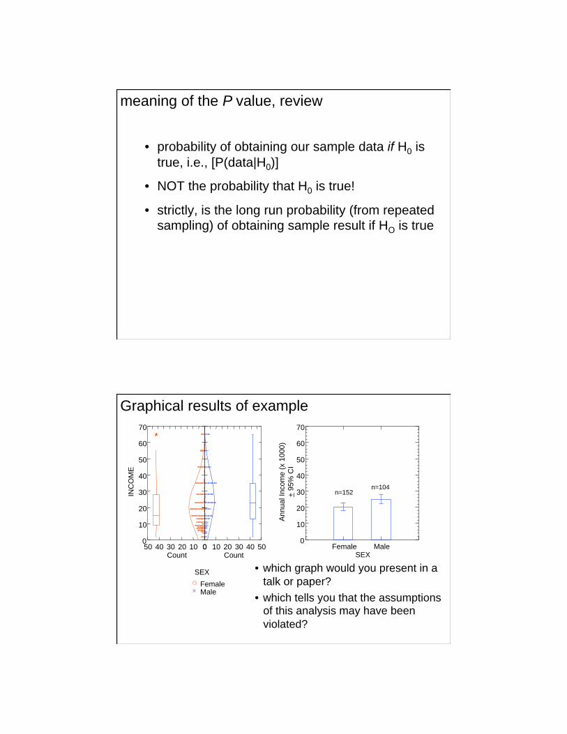
Two-sample t-test on INCOME Grouped by SEX$ vs Alternative = 'not equal'

Standard

GROUP N Mean Deviation

-------+---------------------------

Female 152 20.25658 14.82771

Male 104 24.97115 16.41776

Separate Variance

Difference in Means : -4.71457

95.00% Confidence Interval : -8.67643 to -0.75272

t : -2.34611

df : 206.23313

p-value : 0.01992

Pooled Variance



t : -2.39138

df : 254.00000

p-value : 0.01751

The separate variance t-test is based

on the Satterthwaite adjustment (of degrees of freedom), it is not

recommended unless the variance terms are very different and the

sample sizes (n) are very different

What is the conclusion?

Results of example

• probability of obtaining our sample data if H0 is

true, i.e., [P(data|H0)]

• NOT the probability that H0 is true!

• strictly, is the long run probability (from repeated

sampling) of obtaining sample result if HO is true

meaning of the P value, review

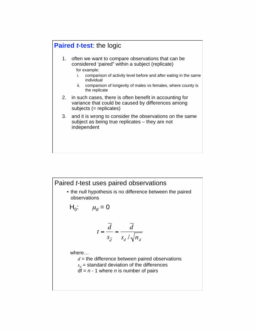
Male Female

SEX

0

10

20

30

40

50

60

70

INC

OM

E

0 10 20 30 40 50 Count

0 10 20 30 40 50 Count

Female Male SEX

0

10

20

30

40

50

60

70

Annual In

com

e (

x 1

000)

+ 9

5%

CI

n=152 n=104

Graphical results of example

• which graph would you present in a

talk or paper?

• which tells you that the assumptions of this analysis may have been

violated?

1. often we want to compare observations that can be considered ‘paired” within a subject (replicate)

for example:

i. comparison of activity level before and after eating in the same individual

ii. comparison of longevity of males vs females, where county is the replicate

2. in such cases, there is often benefit in accounting for variance that could be caused by differences among subjects (= replicates)

3. and it is wrong to consider the observations on the same subject as being true replicates – they are not independent

Paired t-test: the logic

Paired t-test uses paired observations

H0: μd = 0

where…

d = the difference between paired observations

sd = standard deviation of the differences df = n - 1 where n is number of pairs

• the null hypothesis is no difference between the paired

observations

t =d

sd

=d

sd / nd

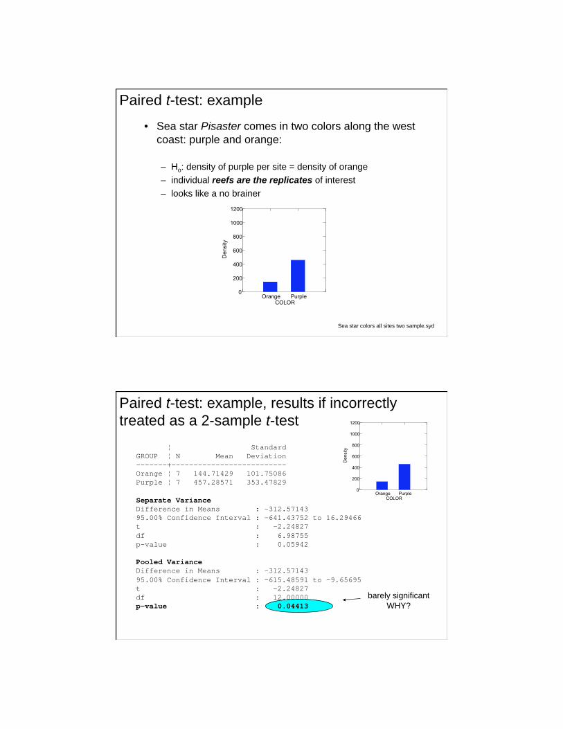
• Sea star Pisaster comes in two colors along the west

coast: purple and orange:

– Ho: density of purple per site = density of orange

– individual reefs are the replicates of interest

– looks like a no brainer

Sea star colors all sites two sample.syd

Paired t-test: example

barely significant

WHY?

Standard

GROUP N Mean Deviation

-------+--------------------------

Orange 7 144.71429 101.75086

Purple 7 457.28571 353.47829

Separate Variance


95.00% Confidence Interval : -641.43752 to 16.29466

t : -2.24827

df : 6.98755

p-value : 0.05942

Pooled Variance



t : -2.24827

df : 12.00000

p-value : 0.04413

Paired t-test: example, results if incorrectly

treated as a 2-sample t-test

Orange Purple Color of seastars

0

200

400

600

800

1000

1200

Density (

95%

CI)

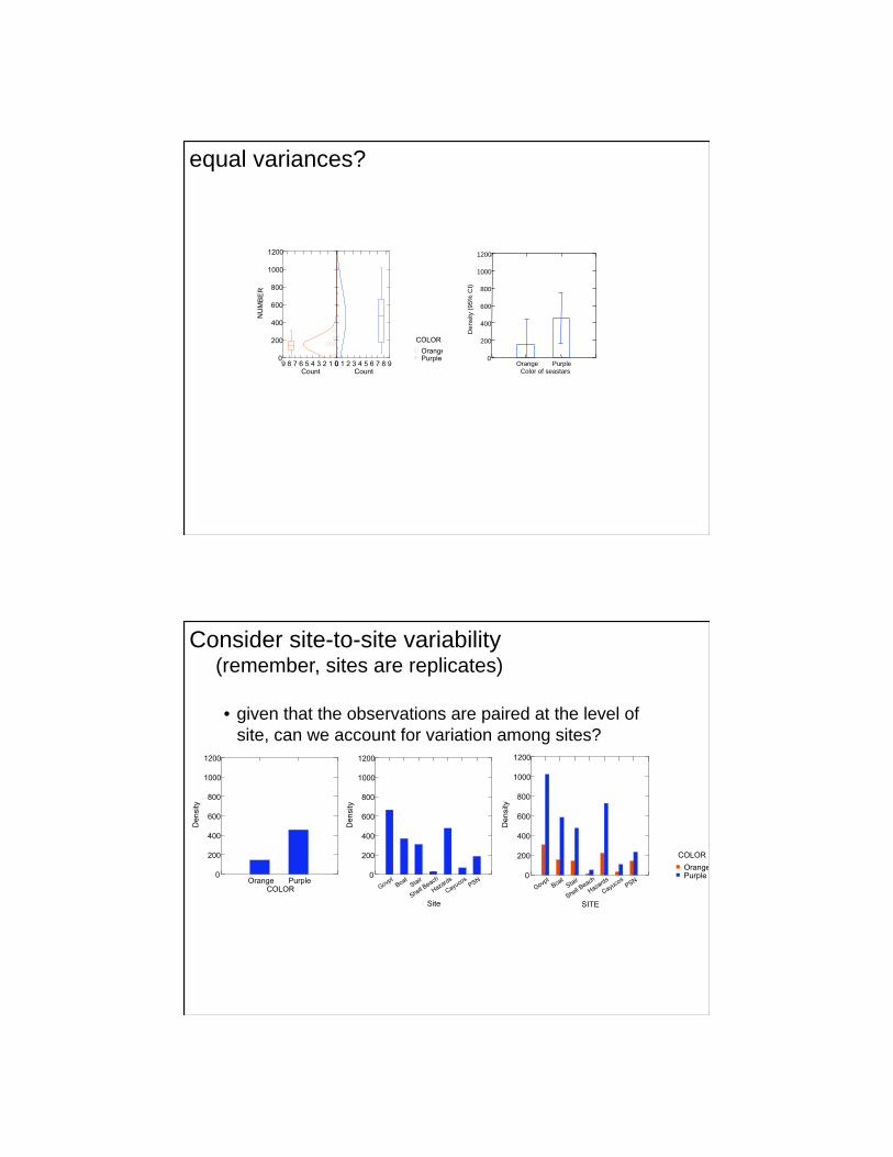
equal variances?

• given that the observations are paired at the level of

site, can we account for variation among sites?

Consider site-to-site variability (remember, sites are replicates)

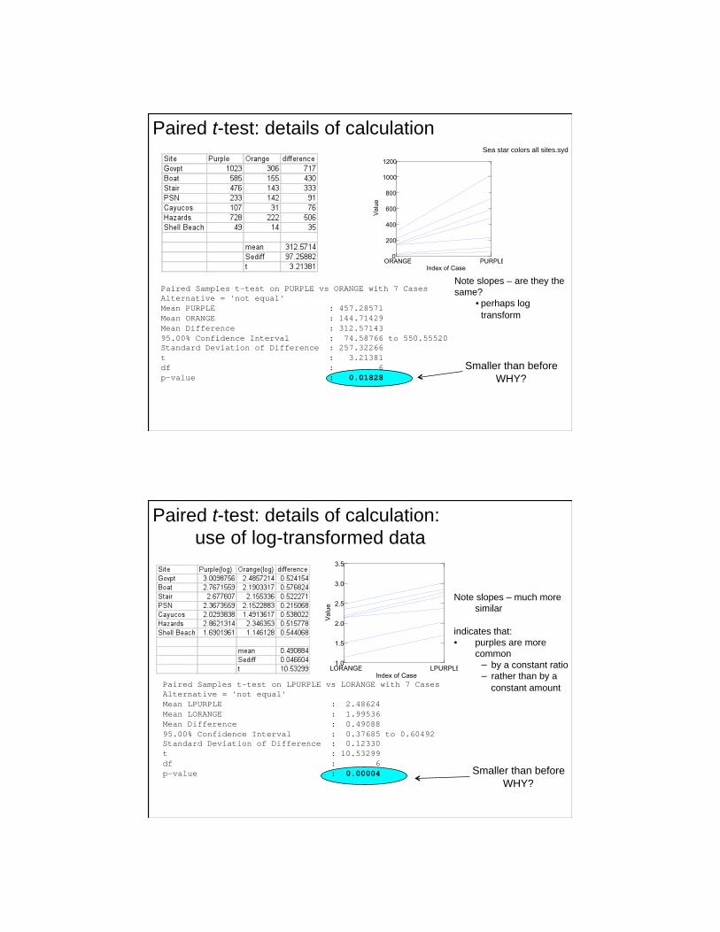
Note slopes – are they the

same?

• perhaps log

transform

Sea star colors all sites.syd

Paired Samples t-test on PURPLE vs ORANGE with 7 Cases Alternative = 'not equal'

Mean PURPLE : 457.28571

Mean ORANGE : 144.71429

Mean Difference : 312.57143

95.00% Confidence Interval : 74.58766 to 550.55520 Standard Deviation of Difference : 257.32266

t : 3.21381

df : 6

p-value : 0.01828

Paired t-test: details of calculation

Smaller than before

WHY?

Note slopes – much more

similar

indicates that:

• purples are more

common

by a constant ratio

rather than by a

constant amount Paired Samples t-test on LPURPLE vs LORANGE with 7 Cases Alternative = 'not equal'

Mean LPURPLE : 2.48624

Mean LORANGE : 1.99536

Mean Difference : 0.49088

95.00% Confidence Interval : 0.37685 to 0.60492 Standard Deviation of Difference : 0.12330

t : 10.53299

df : 6

p-value : 0.00004

Paired t-test: details of calculation:

use of log-transformed data

Smaller than before

WHY?

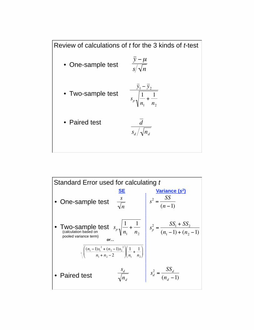
• One-sample test

• Two-sample test

• Paired test

y μ

s n

Review of calculations of t for the 3 kinds of t-test

d

sd nd

y 1 y 2

sp

1n1+1n2

Standard Error used for calculating t

• One-sample test

• Two-sample test

• Paired test

(calculation based on

pooled variance term)

SE Variance (s2)

s

ns2 =

SS

(n 1)

sp1

n1+1

n2sp2=

SS1 + SS2(n1 1) + (n2 1)

sd2=

SSd(nd 1)

sdnd

(n1 1)s12

+ (n2 1)s22

n1 + n2 2

1

n1+1

n2

or…

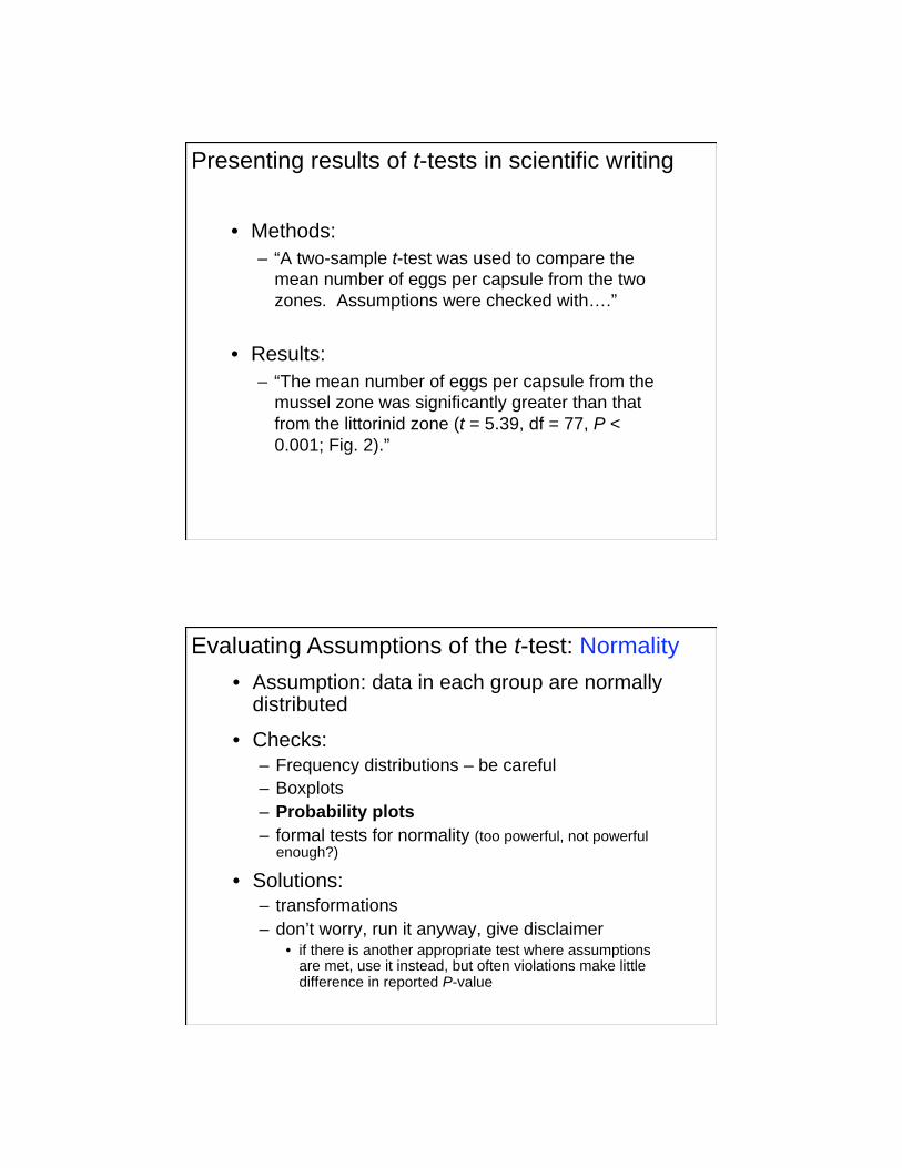
• Methods:

– “A two-sample t-test was used to compare the

mean number of eggs per capsule from the two

zones. Assumptions were checked with….”

• Results:

– “The mean number of eggs per capsule from the

mussel zone was significantly greater than that

from the littorinid zone (t = 5.39, df = 77, P <

0.001; Fig. 2).”

Presenting results of t-tests in scientific writing

• Assumption: data in each group are normally distributed

• Checks:

– Frequency distributions – be careful

– Boxplots

– Probability plots

– formal tests for normality (too powerful, not powerful enough?)

• Solutions: – transformations

– don’t worry, run it anyway, give disclaimer • if there is another appropriate test where assumptions

are met, use it instead, but often violations make little difference in reported P-value

Evaluating Assumptions of the t-test: Normality

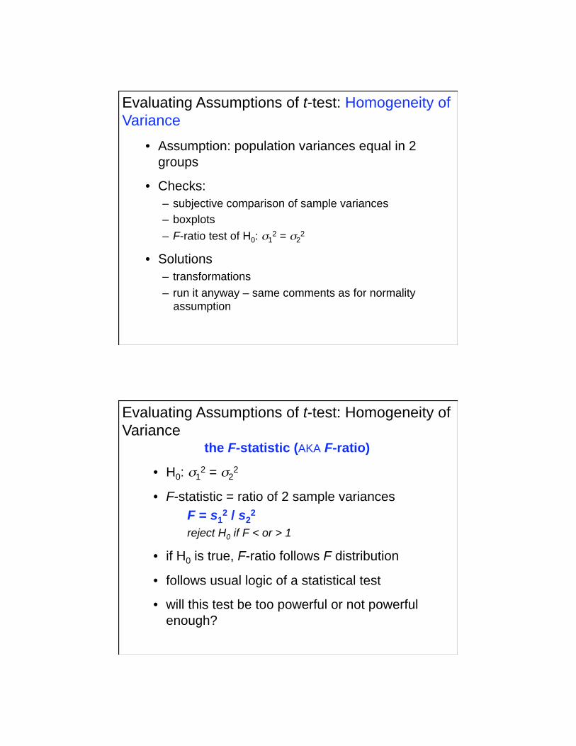
• Assumption: population variances equal in 2

groups

• Checks:

– subjective comparison of sample variances

– boxplots

– F-ratio test of H0: 12 = 2

2

• Solutions

– transformations

– run it anyway – same comments as for normality

assumption

Evaluating Assumptions of t-test: Homogeneity of

Variance

• H0: 12 = 2

2

• F-statistic = ratio of 2 sample variances

F = s12 / s2

2

reject H0 if F < or > 1

• if H0 is true, F-ratio follows F distribution

• follows usual logic of a statistical test

• will this test be too powerful or not powerful

enough?

Evaluating Assumptions of t-test: Homogeneity of

Variance the F-statistic (AKA F-ratio)

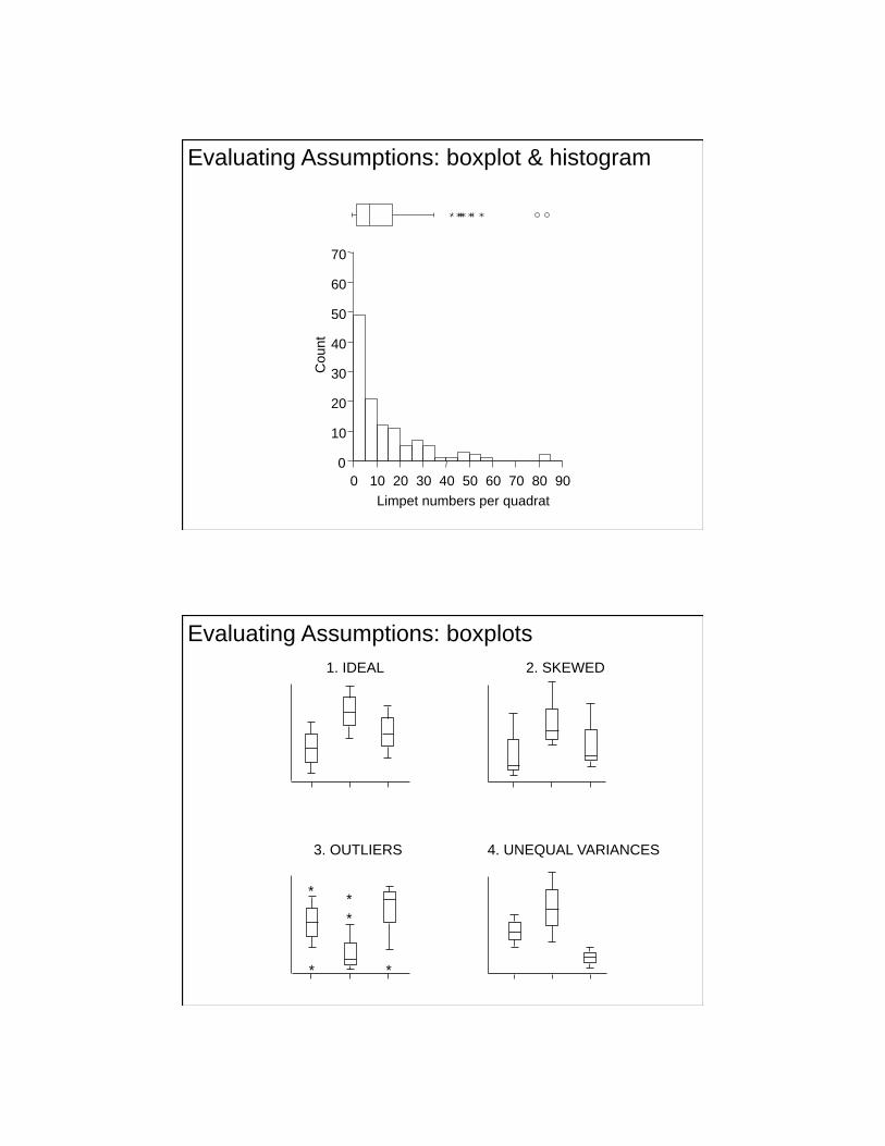
0 10 20 30 40 50 60 70 80 90

Limpet numbers per quadrat

0

10

20

30

40

50

60

70

Count

Evaluating Assumptions: boxplot & histogram

1. IDEAL 2. SKEWED

4. UNEQUAL VARIANCES 3. OUTLIERS

*

*

*

*

*

Evaluating Assumptions: boxplots

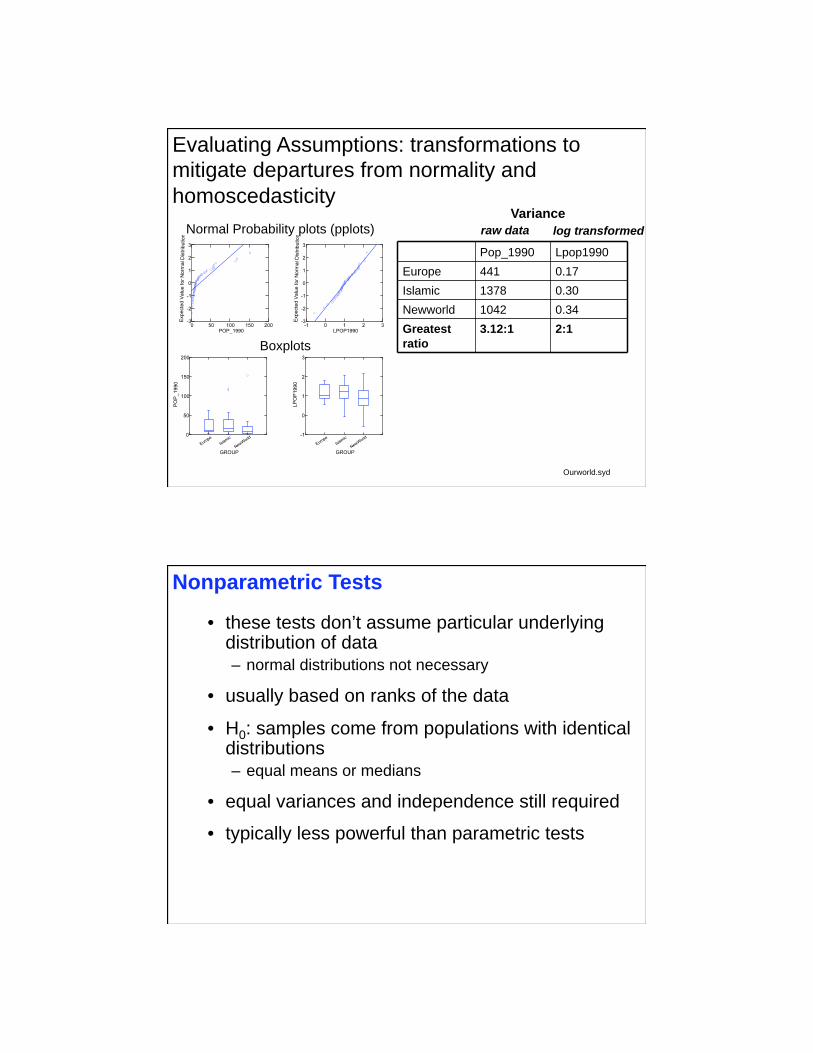
Ourworld.syd

Pop_1990 Lpop1990

Europe 441 0.17

Islamic 1378 0.30

Newworld 1042 0.34

Greatest

ratio

3.12:1 2:1

Variance

Evaluating Assumptions: transformations to

mitigate departures from normality and

homoscedasticity

raw data log transformed Normal Probability plots (pplots)

Boxplots

• these tests don’t assume particular underlying distribution of data – normal distributions not necessary

• usually based on ranks of the data

• H0: samples come from populations with identical distributions – equal means or medians

• equal variances and independence still required

• typically less powerful than parametric tests

Nonparametric Tests

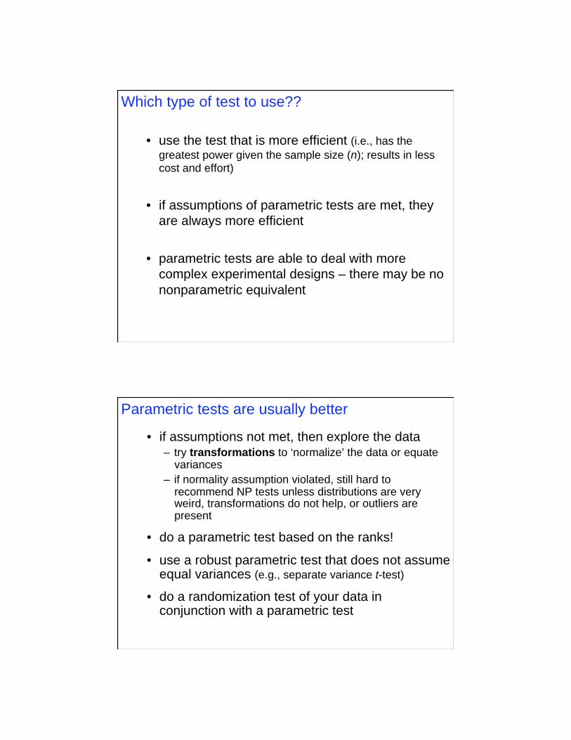
• use the test that is more efficient (i.e., has the

greatest power given the sample size (n); results in less cost and effort)

• if assumptions of parametric tests are met, they

are always more efficient

• parametric tests are able to deal with more

complex experimental designs – there may be no

nonparametric equivalent

Which type of test to use??

• if assumptions not met, then explore the data – try transformations to ‘normalize’ the data or equate

variances

– if normality assumption violated, still hard to recommend NP tests unless distributions are very weird, transformations do not help, or outliers are present

• do a parametric test based on the ranks!

• use a robust parametric test that does not assume equal variances (e.g., separate variance t-test)

• do a randomization test of your data in conjunction with a parametric test

Parametric tests are usually better

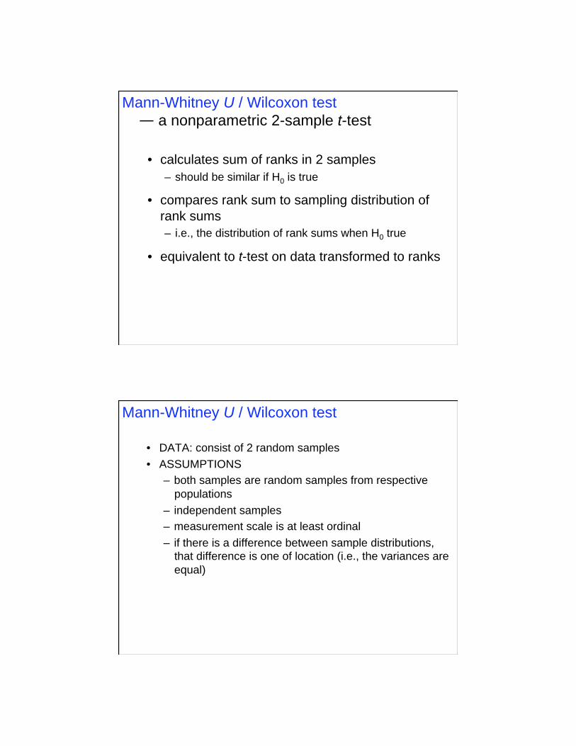
• calculates sum of ranks in 2 samples

– should be similar if H0 is true

• compares rank sum to sampling distribution of

rank sums

– i.e., the distribution of rank sums when H0 true

• equivalent to t-test on data transformed to ranks

Mann-Whitney U / Wilcoxon test

— a nonparametric 2-sample t-test

• DATA: consist of 2 random samples

• ASSUMPTIONS

– both samples are random samples from respective

populations

– independent samples

– measurement scale is at least ordinal

– if there is a difference between sample distributions,

that difference is one of location (i.e., the variances are

equal)

Mann-Whitney U / Wilcoxon test

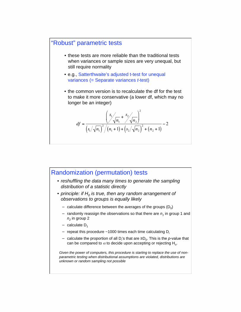
• e.g., Satterthwaite’s adjusted t-test for unequal

variances (= Separate variances t-test)

• the common version is to recalculate the df for the test

to make it more conservative (a lower df, which may no

longer be an integer)

df =

s1n1

+s2

n2

2

s1 n1( )2

n1 +1( ) + s2 n2( )2

+ n2 +1( )2

• these tests are more reliable than the traditional tests

when variances or sample sizes are very unequal, but

still require normality

“Robust” parametric tests

calculate difference between the averages of the groups (D0)

randomly reassign the observations so that there are n1 in group 1 and

n2 in group 2

calculate D1

repeat this procedure ~1000 times each time calculating Di

calculate the proportion of all Di’s that are D0. This is the p-value that

can be compared to to decide upon accepting or rejecting Ho.

Given the power of computers, this procedure is starting to replace the use of non-

parametric testing when distributional assumptions are violated, distributions are unknown or random sampling not possible

• reshuffling the data many times to generate the sampling

distribution of a statistic directly

• principle: if H0 is true, then any random arrangement of observations to groups is equally likely

Randomization (permutation) tests

Documents

6_Introduction to Hypothesis Testing_2012