A family of multivariate χ2-statistics

Discrete Math. Appl., Vol. 14, No. 5, pp. 527–533 (2004)© VSP 2004.

A family of multivariate χ 2-statistics

B. I. SELIVANOV

Abstract — We consider a sequence of independent trials, under the hypothesis H0 each of themis a realisation of a certain polynomial scheme. We introduce a family of multivariate χ2-statisticswhere the outcomes are equipped with weights depending on the ordinal of the trial. Earlier results onfamilies of multivariate χ2-statistic are extended to this family.

This research was supported by grant 1758.2003.1 of President of Russian Federation for supportof leading scientific schools.

1. INTRODUCTION

Let

X1, X2, . . . , Xn . . . (1)

be a sequence of independent random variables whose values are elements of the set{1, . . . , N}; it is assumed that N is fixed. In what follows, for random variables (1) weuse the Kolmogorov notation [1] and speak about independent trials with possible outcomes1, . . . , N . By the null hypothesis H0, each of trials (1) is carried out according to thesame polynomial scheme with probabilities of outcomes, respectively, p 1, . . . , pN , where0 < pi < 1, i = 1, . . . , N , p1 + . . . + pN = 1.

We introduce r sequences of real numbers

ak(1), ak(2), . . . , ak(n), . . . , k = 1, . . . , r. (2)

Let ak(t) mean the kth weight of outcomes in the t th trial. We introduce the random vari-ables

Rki (n) =n∑

t=1

ak(t)I {Xt = i}, k = 1, . . . , r, i = 1, . . . , N,

where I {Xt = i} is the indicator of the event {X t = i}, and

ξki = 1√A(2)

k (n)pi

(Rki (n) − A(1)k (n)pi), i = 1, . . . , r, i = 1, . . . , N, (3)

Originally published in Diskretnaya Matematika (2004) 16, No. 4 (in Russian).Received November 12, 2003.

528 B. I. Selivanov

where

A(1)k (n) =

n∑

t=1

ak(t), A(2)k (n) =

N∑

t=1

a2k (t). (4)

With the use of random variables (3) we define the r -variate χ 2-statistic

χ2 = (χ21 , . . . , χ2

r ) (5)

with the components

χ2k =

N∑

i=1

ξ2ki =

N∑

i=1

1

A(2)k (n)pi

(Rki (n) − A(1)k (n)pi )

2, k = 1, . . . , r, (6)

depending on the choice of weights (2). By varying sequences (2), we get a family ofr -dimensional χ 2-statistics.

The family obtained includes the family of r -dimensional χ 2-statistics introduced in[2]. Let A1, . . . , Ar be finite non-empty sets of positive integers. We define the outcomeweights for k = 1, . . . , r and t = 1, . . . , n as ak(t) = 1 if t ∈ Ak and ak(t) = 0 otherwise.Then statistic (5) with components (6) is precisely the r -dimensional χ 2-statistic in [2]whose particular cases were considered in papers [3, 4].

In this paper, the results obtained in [2] for ordinary χ 2-statistics are extended to thegeneralised χ 2-statistics (as concerns univariate χ 2-statistics, see [5]). In Section 2, we giveauxiliary results used to prove two limit theorems on statistics (5) formulated in Section 3.They state that there are limit distributions for statistics (5) both under the null hypothesisH0 and under the contigual to it alternatives. We also obtain representations of the Laplacetransforms of the limit distributions belonging to the class of multivariate χ 2 distributionsdefined in [2]. The technique used in [2] can be applied to the case considered here, whichallows us to restrict ourselves to formulations of the results only.

2. AUXILIARY RESULTS

We consider the sequence of vectors

p = (p1, . . . , pn), (7)

where

pt = (p1(t), . . . , pN (t)), 0 ≤ pi (t) < 1, i = 1, . . . , N,

N∑

i=1

pi(t) = 1 (8)

for t = 1, . . . , n.We say that trials (1) satisfy a (simple) hypothesis H (p) if polynomial scheme (8)

is realised in the t th trial, t = 1, . . . , n. In the case p1 = . . . = pn = p, wherep = (p1, . . . , pN ), the hypothesis H0 is satisfied. If pt �= p in (7) for some t = 1, . . . , n,then the hypothesis H (p) is said to be alternative to H0.

The three lemmas below extend the corresponding Lemmas 1, 2, 3 in [2]. First, with theuse of the random variables Rki (n) introduced in Section 1 we prove the following assertion.

A family of multivariate χ2-statistics 529

Lemma 1. If trials (1) are carried out under the condition that the hypothesis H (p)

defined by sequence (7) of polynomial schemes (8) is true, then for random variables (3)

Eξki = 1√A(2)

k (n)pi

n∑

t=1

ak(t)(pi (t) − pi ), (9)

cov(ξki , ξl j ) =∑n

t=1 ak(t)al(t)√

pi(t)pj (t)√A(2)

k (n)A(2)l (n)pi pj

(δi j −√

pi(t)pj (t)), (10)

where δi j is the Kronecker delta, k, l = 1, . . . , r, i, j = 1, . . . , N.

Corollary 1. If the hypothesis H0 is true, then

Eξki = 0, cov(ξki , ξl j ) = �kl(n)(δi j − √pi pj ), (11)

where

�kl(n) =∑n

t=1 ak(t)al(t)√A(2)

k (n)A(2)l (n)

, k, l = 1, . . . , r, i, j = 1, . . . , N . (12)

Lemma 1 and Corollary 1 in [2] are particular cases of formulas (9)–(12).Let the length n of sequence (1) grow without bound. The sequence {a(t)} n

t=1 of realnumbers, as in [5], is said to be regular if the relation

max1≤t≤n

a2(t)

/n∑

t=1

a2(t) = o(1) (13)

holds as n → ∞. Condition (F1) in [2] is a particular case of this condition.Before formulating the next lemma, we introduce the r N-dimensional vector

ξ = (ξ11, . . . , ξ1N ; . . . ; ξr1, . . . , ξr N ) (14)

whose components are random variables (3).

Lemma 2. Let trials (1) be carried out under the condition that the hypothesis H 0 istrue, all r sequences of weights of outcomes (2) be regular, and let variables (12) have thelimits

limn→∞ �kl(n) = ρkl , k, l = 1, . . . , r. (15)

Then random vector (14), as n → ∞, converges in distribution to the r N-dimensionalnormal random vector

ξ = (ξ(1)11 , . . . , ξ

(1)1N ; . . . ; ξ

(1)r1 , . . . , ξ

(1)r N ) (16)

with zero vector of means and the covariance matrix D = ‖dki,l j ‖ of order r N whoseelements are

dki,l j = ρkl(δi j − √pi pj ), k, l = 1, . . . , r, i, j = 1, . . . , N .

530 B. I. Selivanov

This lemma extends Lemma 2 in [2] and Theorem 3.2 in [5]. Similarly to those as-sertions in [2, 5], it immediately follows from the multidimensional central limit theorem.Instead of Lemma 2, it is possible to formulate a more strong assertion similar to Lemma 3.3in [5]. We also observe that condition (F2) in [2] is a particular case of condition (15).

In what follows, as in [2], we consider only those alternatives H (p) to the null hypo-thesis which are contigual to H0 in the LeCam sense ([6], Chapter 6). It is known [5] thatthe alternative H (p) is contigual to H0 if and only if the condition

limn→∞ sup

n∑

t=1

N∑

i=1

(pi(t) − pi )2

pi< ∞ (17)

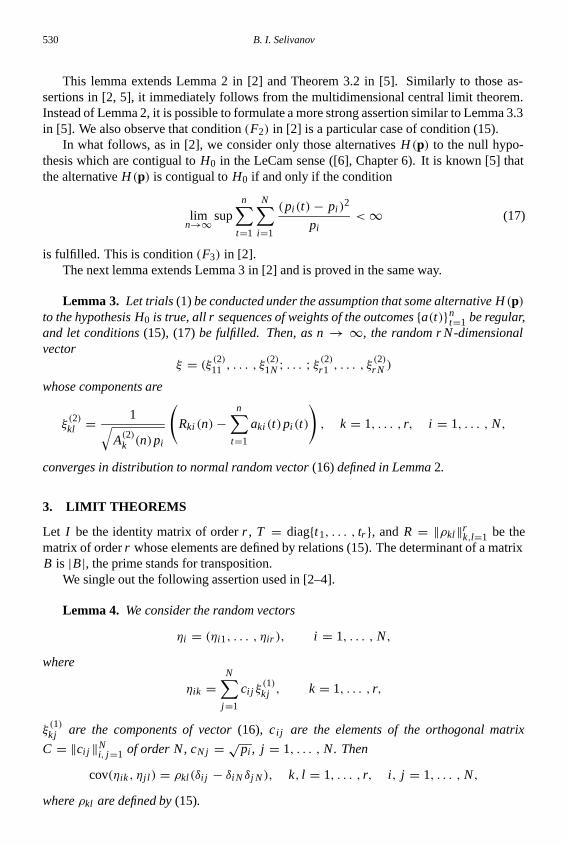
is fulfilled. This is condition (F3) in [2].The next lemma extends Lemma 3 in [2] and is proved in the same way.

Lemma 3. Let trials (1) be conducted under the assumption that some alternative H (p)

to the hypothesis H0 is true, all r sequences of weights of the outcomes {a(t)}nt=1 be regular,

and let conditions (15), (17) be fulfilled. Then, as n → ∞, the random r N-dimensionalvector

ξ = (ξ(2)11 , . . . , ξ

(2)1N ; . . . ; ξ

(2)r1 , . . . , ξ

(2)r N )

whose components are

ξ(2)kl = 1√

A(2)k (n)pi

(Rki (n) −

n∑

t=1

aki (t)pi (t)

), k = 1, . . . , r, i = 1, . . . , N,

converges in distribution to normal random vector (16) defined in Lemma 2.

3. LIMIT THEOREMS

Let I be the identity matrix of order r , T = diag{t1, . . . , tr }, and R = ‖ρkl‖rk,l=1 be the

matrix of order r whose elements are defined by relations (15). The determinant of a matrixB is |B|, the prime stands for transposition.

We single out the following assertion used in [2–4].

Lemma 4. We consider the random vectors

ηi = (ηi1, . . . , ηir ), i = 1, . . . , N,

where

ηik =N∑

j=1

ci j ξ(1)kj , k = 1, . . . , r,

ξ(1)kj are the components of vector (16), ci j are the elements of the orthogonal matrix

C = ‖ci j ‖Ni, j=1 of order N, cN j = √

pi , j = 1, . . . , N. Then

cov(ηik , ηj l) = ρkl(δi j − δiN δj N ), k, l = 1, . . . , r, i, j = 1, . . . , N,

where ρkl are defined by (15).


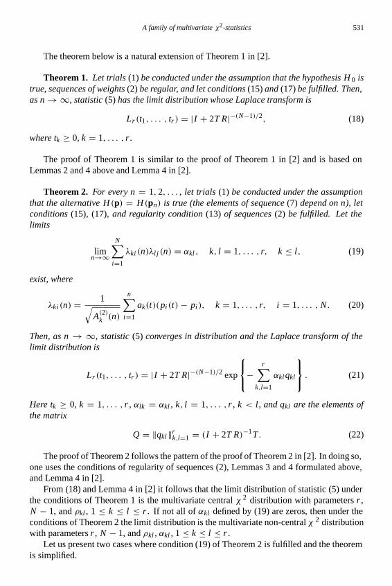
The theorem below is a natural extension of Theorem 1 in [2].

Theorem 1. Let trials (1) be conducted under the assumption that the hypothesis H 0 istrue, sequences of weights (2) be regular, and let conditions (15) and (17) be fulfilled. Then,as n → ∞, statistic (5) has the limit distribution whose Laplace transform is

Lr (t1, . . . , tr ) = |I + 2T R|−(N−1)/2, (18)

where tk ≥ 0, k = 1, . . . , r .

The proof of Theorem 1 is similar to the proof of Theorem 1 in [2] and is based onLemmas 2 and 4 above and Lemma 4 in [2].

Theorem 2. For every n = 1, 2, . . . , let trials (1) be conducted under the assumptionthat the alternative H (p) = H (pn) is true (the elements of sequence (7) depend on n), letconditions (15), (17), and regularity condition (13) of sequences (2) be fulfilled. Let thelimits

limn→∞

N∑

i=1

λki (n)λl j (n) = αkl , k, l = 1, . . . , r, k ≤ l, (19)

exist, where

λki (n) = 1√A(2)

k (n)

n∑

t=1

ak(t)(pi (t) − pi ), k = 1, . . . , r, i = 1, . . . , N . (20)

Then, as n → ∞, statistic (5) converges in distribution and the Laplace transform of thelimit distribution is

Lr (t1, . . . , tr ) = |I + 2T R|−(N−1)/2 exp

−r∑

k,l=1

αklqkl

. (21)

Here tk ≥ 0, k = 1, . . . , r , αlk = αkl , k, l = 1, . . . , r , k < l, and qkl are the elements ofthe matrix

Q = ‖qkl‖rk,l=1 = (I + 2T R)−1T . (22)

The proof of Theorem 2 follows the pattern of the proof of Theorem 2 in [2]. In doing so,one uses the conditions of regularity of sequences (2), Lemmas 3 and 4 formulated above,and Lemma 4 in [2].

From (18) and Lemma 4 in [2] it follows that the limit distribution of statistic (5) underthe conditions of Theorem 1 is the multivariate central χ 2 distribution with parameters r ,N − 1, and ρkl , 1 ≤ k ≤ l ≤ r . If not all of αkl defined by (19) are zeros, then under theconditions of Theorem 2 the limit distribution is the multivariate non-central χ 2 distributionwith parameters r , N − 1, and ρkl , αkl , 1 ≤ k ≤ l ≤ r .

Let us present two cases where condition (19) of Theorem 2 is fulfilled and the theoremis simplified.

532 B. I. Selivanov

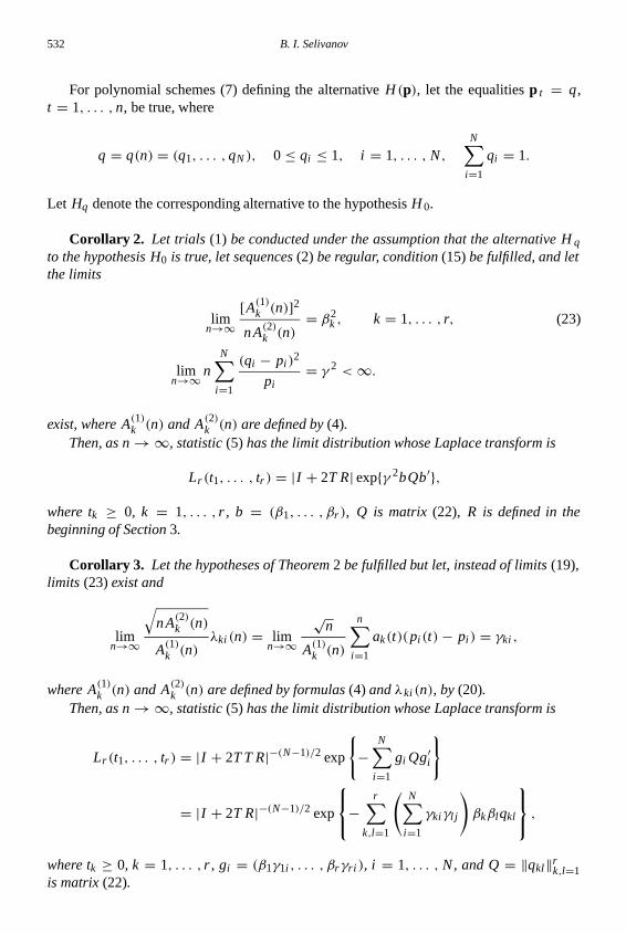
For polynomial schemes (7) defining the alternative H (p), let the equalities p t = q,t = 1, . . . , n, be true, where

q = q(n) = (q1, . . . , qN ), 0 ≤ qi ≤ 1, i = 1, . . . , N,

N∑

i=1

qi = 1.

Let Hq denote the corresponding alternative to the hypothesis H 0.

Corollary 2. Let trials (1) be conducted under the assumption that the alternative H q

to the hypothesis H0 is true, let sequences (2) be regular, condition (15) be fulfilled, and letthe limits

limn→∞

[A(1)k (n)]2

nA(2)k (n)

= β2k , k = 1, . . . , r, (23)

limn→∞ n

N∑

i=1

(qi − pi )2

pi= γ 2 < ∞.

exist, where A(1)k (n) and A(2)

k (n) are defined by (4).Then, as n → ∞, statistic (5) has the limit distribution whose Laplace transform is

Lr (t1, . . . , tr ) = |I + 2T R| exp{γ 2bQb′},

where tk ≥ 0, k = 1, . . . , r , b = (β1, . . . , βr ), Q is matrix (22), R is defined in thebeginning of Section 3.

Corollary 3. Let the hypotheses of Theorem 2 be fulfilled but let, instead of limits (19),limits (23) exist and

limn→∞

√nA(2)

k (n)

A(1)k (n)

λki (n) = limn→∞

√n

A(1)k (n)

n∑

i=1

ak(t)(pi (t) − pi ) = γki ,

where A(1)k (n) and A(2)

k (n) are defined by formulas (4) and λki (n), by (20).Then, as n → ∞, statistic (5) has the limit distribution whose Laplace transform is

Lr (t1, . . . , tr ) = |I + 2T T R|−(N−1)/2 exp

{−

N∑

i=1

gi Qg′i

}

= |I + 2T R|−(N−1)/2 exp

−r∑

k,l=1

(N∑

i=1

γkiγl j

)βkβlqkl

,

where tk ≥ 0, k = 1, . . . , r , gi = (β1γ1i , . . . , βrγri ), i = 1, . . . , N, and Q = ‖qkl‖rk,l=1

is matrix (22).


REFERENCES

1. A. N. Kolmogorov, Fundamental Notions of Probability Theory. Nauka, Moscow, 1974 (in Rus-sian).

2. B. I. Selivanov, A family of multivariate χ2-statistics. Discrete Math. Appl. (2002) 12, 401–413.

3. V. K. Zakharov, O. V. Sarmanov, and B. A. Sevastyanov, Sequential χ2 criteria. Math. USSRSbornik (1970) 8, 419–435.

4. M. I. Tikhomirova, and V. P. Chistyakov, A moving chi-square. Discrete Math. Appl. (2000) 10,469–475.

5. B. I. Selivanov, On a class of chi-square statistics. Review of Applied and Industrial Math. (1995)2, 926–966 (in Russian).

6. J. Hajek and Z. Sidak, Theory of Rank Tests. Academic Press, New York, 1967.

Documents

A family of multivariate χ2-statistics