Alisha Thesis

8/7/2019 Alisha Thesis

http://slidepdf.com/reader/full/alisha-thesis 1/41

Design of a Single Orice Pulse Tube Refrigerator Through theDevelopment of a First-Order Model

by

Alisha R. Schor

Submitted to the Department of MechanicalEngineering in Partial Fulllment of the

Requirements for the Degree of

Bachelor of Science

at the

Massachusetts Institute of Technology

June 2007

c Alisha SchorAll Rights Reserved

The author hereby grants to MIT permission to reproduce and to distributepublicly paper and electronic copies of this thesis document in whole or

in part in any medium now known or hereafter created.

Signature of Author................................................................................................................................Department of Mechanical Engineering

May 11, 2007

Certied by.............................................................................................................................................John G. Brisson, IIAssociate Professor

Thesis Supervisor

Accepted by.............................................................................................................................................John H. Lienhard

Professor, ME Undergraduate Officer

1



(This page intentionally left blank)

2



Abstract

A rst order model for the behavior of a linear orice pulse tube refrigerator (OPTR) was devel-

oped as a design tool for construction of actual OPTRs. The model predicts cooling power as well as

the pressure/volume relationships for various segments of the refrigerator with minimal computational

requirements. The rst portion of this document describes the development of this model and its sim-

plications relative to higher-order numerical models. The second portion of this document details a

physical implementation of the pulse tube and compares its performance to the predicted performance

of the model. It was found that the model accurately predicted qualitative behavior and trends of the

orice pulse tube refrigerator, but that the predicted temperature difference was approximately ve times

higher than the measured temperature difference. It is believed that the model can be improved with

provisions for ow choking as well as warnings for behavior outside of the accepted operating conditions.

3



Acknowledgements

I would like to graciously acknowledge the help of Professor John Brisson, who encouraged me through my

work and always took the time to have casual and engaging discussions as well. Professor Joseph Smith was

also invaluable in contributing his wisdom and experience to the project, as well as Mr. Michael Demaree,who was generous with his time and knowledge in the machine shop.

4



Contents

1 Introduction 6

1.1 Single Orice Pulse Tube Refrigerator (OPTR) . . . . . . . . . . . . . . . . . . . . . . . . . . 6

1.2 Existing OPTRs and their applications . . . . . . . . . . . . . . . . . . . . . . . . . . . . . . . 7

2 Model 8

2.1 The First-Order Model . . . . . . . . . . . . . . . . . . . . . . . . . . . . . . . . . . . . . . . . 9

2.2 Limitations of the Model . . . . . . . . . . . . . . . . . . . . . . . . . . . . . . . . . . . . . . . 15

3 Design of Physical System 15

3.1 Fabrication . . . . . . . . . . . . . . . . . . . . . . . . . . . . . . . . . . . . . . . . . . . . . . 18

3.2 Testing . . . . . . . . . . . . . . . . . . . . . . . . . . . . . . . . . . . . . . . . . . . . . . . . 19

4 Results 20

5 Discussion 24

6 Conclusion 29

A Isentropic relations for density 30

B Phase shift relationships 31

C Gas compression work 34

D MATLAB Code 35

5



1 Introduction

The pulse tube refrigerator is one of the most prominent types of cryocoolers available today, due to its

simplicity and ability to achieve cryogenic temperatures. Several forms of pulse-tube refrigerators exist, but

all operate on the Stirling refrigeration cycle and contain the same basic elements: a pressure oscillator,hot and cold heat exchangers, a Stirling-type regenerator, a pulse tube, and a pressure reservoir. Variations

between refrigerators can come in the shape and orientation of the pulse tube, the choice of working uid,

the pressure source, and the gas ow path. Pulse tube refrigerators also exist in either single or double orice

varieties, the latter of which allows a small fraction of gas to bypass the regenerator, reducing losses due to

pressure drop [1]. Discussion in this document will be limited to the single orice pulse tube refrigerator

(OPTR).

1.1 Single Orice Pulse Tube Refrigerator (OPTR)

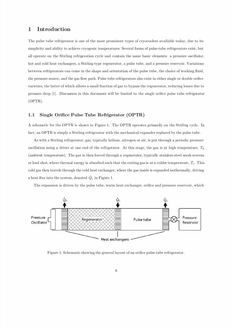
A schematic for the OPTR is shown in Figure 1. The OPTR operates primarily on the Stirling cycle. In

fact, an OPTR is simply a Stirling refrigerator with the mechanical expander replaced by the pulse tube.

As with a Stirling refrigerator, gas, typically helium, nitrogen or air, is put through a periodic pressure

oscillation using a driver at one end of the refrigerator. At this stage, the gas is at high temperature, T h

(ambient temperature). The gas is then forced through a regenerator, typically stainless steel mesh screens

or lead shot, where thermal energy is absorbed such that the exiting gas is at a colder temperature, T c . This

cold gas then travels through the cold heat exchanger, where the gas inside is expanded isothermally, driving

a heat ux into the system, denoted Qc in Figure 1.

The expansion is driven by the pulse tube, warm heat exchanger, orice and pressure reservoir, which

Figure 1: Schematic showing the general layout of an orice pulse tube refrigerator.

6



make up the remainder of the system. The orice provides a resistance to the gas ow; the pressure reservoir

is a capacitive element. Together, these create an effective spring-mass-damper system and create a phase

shift between mass ow rate and pressure. The heat exchanger between the pulse tube and the throttle is

included to dissipate the entropy generated in the throttle.

The pressure reservoir is designed with a volume large enough such that it remains at an average pressure,

P o , throughout the pressure cycles of the refrigerator. The orice, meanwhile, is sized to decrease the ow

between the pulse tube and pressure reservoir, ensuring that not all of the gas in the pulse tube is forced

out of the tube. The pulse tube is the primary component of this system. It is designed with sufficient

length such that an oscillating slug of gas maintains a separation between the warm and cold ends of the

refrigerator. With the aid of ow straighteners, this slug of gas can be viewed as essentially unmixed with the

gases at either end, and the result is that the oscillating gas through the orice/pressure reservoir appears to

behave in the same way that a mechanical expander would in a traditional Stirling refrigerator. (It should

also be noted that early pulse tube refrigerators relied the heat generated in and dissipated out of the pulse

tube only to create a phase shift, without the aid of the orice and pressure reservoir.) Further detail on the

behavior of each component in the OPTR is described in Section 2.

1.2 Existing OPTRs and their applications

Due to their high efficiency at large temperature differences, pulse tube refrigerators are frequently used in

cryocooling applications. Early on, the most prominent use of pulse tube refrigerators was by the military,

to cool infared cameras [1]. Currently, a number of research institutes (primarily Lockheed Martin, National

Institute of Standards and Technology-NIST and Los Alamos National Labs [1]) pursue the development of

pulse tube cryocoolers for academic interest, as well as for applications in space. Commercial applications

include refrigeration of charcoal adsorbent beds in the semiconductor fabrication industry [1] as well as the

liquefaction of helium and nitrogen, for various applications. In many cases, pulse tube refrigerators are

being explored as alternatives to current cryocoolers, as they have the advantage of having no moving parts

at low temperatures.

7



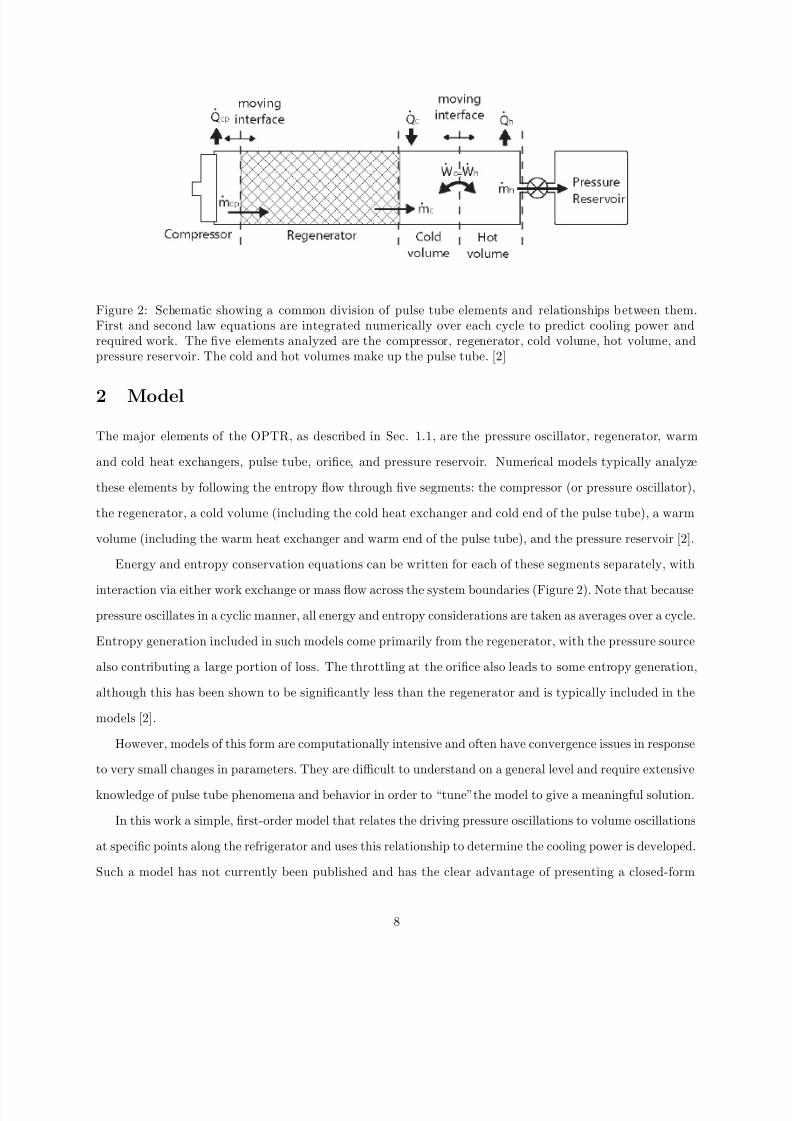
Figure 2: Schematic showing a common division of pulse tube elements and relationships between them.First and second law equations are integrated numerically over each cycle to predict cooling power andrequired work. The ve elements analyzed are the compressor, regenerator, cold volume, hot volume, andpressure reservoir. The cold and hot volumes make up the pulse tube. [2]

2 Model

The major elements of the OPTR, as described in Sec. 1.1, are the pressure oscillator, regenerator, warm

and cold heat exchangers, pulse tube, orice, and pressure reservoir. Numerical models typically analyze

these elements by following the entropy ow through ve segments: the compressor (or pressure oscillator),

the regenerator, a cold volume (including the cold heat exchanger and cold end of the pulse tube), a warm

volume (including the warm heat exchanger and warm end of the pulse tube), and the pressure reservoir [2].

Energy and entropy conservation equations can be written for each of these segments separately, with

interaction via either work exchange or mass ow across the system boundaries (Figure 2). Note that becausepressure oscillates in a cyclic manner, all energy and entropy considerations are taken as averages over a cycle.

Entropy generation included in such models come primarily from the regenerator, with the pressure source

also contributing a large portion of loss. The throttling at the orice also leads to some entropy generation,

although this has been shown to be signicantly less than the regenerator and is typically included in the

models [2].

However, models of this form are computationally intensive and often have convergence issues in response

to very small changes in parameters. They are difficult to understand on a general level and require extensive

knowledge of pulse tube phenomena and behavior in order to “tune”the model to give a meaningful solution.

In this work a simple, rst-order model that relates the driving pressure oscillations to volume oscillations

at specic points along the refrigerator and uses this relationship to determine the cooling power is developed.

Such a model has not currently been published and has the clear advantage of presenting a closed-form

8



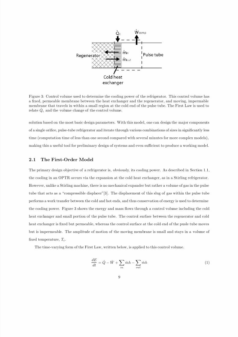
Figure 3: Control volume used to determine the cooling power of the refrigerator. This control volume hasa xed, permeable membrane between the heat exchanger and the regenerator, and moving, impermablemembrane that travels in within a small region at the cold end of the pulse tube. The First Law is used torelate Qc and the volume change of the control volume.

solution based on the most basic design parameters. With this model, one can design the major components

of a single orice, pulse-tube refrigerator and iterate through various combinations of sizes in signicantly less

time (computation time of less than one second compared with several minutes for more complex models),

making this a useful tool for preliminary design of systems and even sufficient to produce a working model.

2.1 The First-Order Model

The primary design objective of a refrigerator is, obviously, its cooling power. As described in Section 1.1,

the cooling in an OPTR occurs via the expansion at the cold heat exchanger, as in a Stirling refrigerator.

However, unlike a Stirling machine, there is no mechanical expander but rather a volume of gas in the pulse

tube that acts as a “compressible displacer”[3]. The displacement of this slug of gas within the pulse tube

performs a work transfer between the cold and hot ends, and thus conservation of energy is used to determine

the cooling power. Figure 3 shows the energy and mass ows through a control volume including the cold

heat exchanger and small portion of the pulse tube. The control surface between the regenerator and cold

heat exchanger is xed but permeable, whereas the control surface at the cold end of the pusle tube moves

but is impermeable. The amplitude of motion of the moving membrane is small and stays in a volume of

xed temperature, T c .

The time-varying form of the First Law, written below, is applied to this control volume.

dE dt

= Q − W +in

mh −out

mh (1)

9



As shown in Figure 3, Q = Qc and W is the rate of expansion work performed by the displacer. The

relationship between (compression or expansion) work , pressure and volume in oscillating ow is a commonly

encountered term and can be expressed as W = 12 P a V a sin (φ), where φ is the phase shift between pressure

and volume ow, and P a and V a represent the amplitudes of oscillation for pressure and volume, respectively.

(For reference, this is derived in Appendix C.) The rate at which work is done is simply W = W × f , where

f is the frequency of oscillation.

Enthalpy ow is considered next. Between the regenerator and the cold heat exchanger, the net enthalpy

ow is zero, even though there is mass ow. In an ideal regenerator the temperature exiting near the cold

heat exchanger is always T c . In addition, the cold heat exchanger is assumed to be isothermal, also at T c .

Thus, assuming that there is no dead space between the regenerator and cold heat exchanger, T out = T in = T c

for the mass ow on the regenerator side of the control volume shown in Figure 3. Also, for an ideal gas,

h = cp T , and therefore hout = h in . Lastly, the cyclic behavior of the system gives that ˙ m in = mout , and

therefore there is no net enthalpy ow between the cold heat exchanger and the regenerator. On the pulse

tube side, since mass ow is zero, there is clearly no enthalpy ow.

Finally, the change in energy over a cycle, dEdt is zero. Substituting, Eq. 1 can be rewritten as

0 = Qc − f 12

P a ∆ V a sin (φ) + 0 (2)

which is easily rearranged to give

Qc = f 12

P a ∆ V a sin (φ) (3)

A similar approach is used to nd the work required to drive the OPTR. In fact, the relationship given

above, W = 12 PV sin (φ), gives the work directly, taking the entire OPTR as the control volume, such that

W = f 12

P a ∆ V a sin (φ) (4)

However, it is important to realize that the volume changes, ∆ V a and phase shifts, φ, between pressure

and volume are not the same for Eqs. 3 and 4. The phase shift between pressure and volume at the inletof the OPTR, used to nd the work, is different than the phase shift at the cold heat exchanger, used to

nd the cooling power, as a result of the compressibility of the working uid. By the same reasoning, the

amplitude of volume oscillations are different at these two points. The following describes how, given a

number of simplifying assumptions, conservation equations can be applied to appropriate control volumes

10



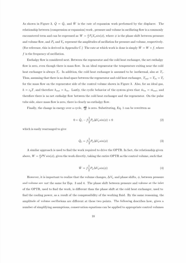
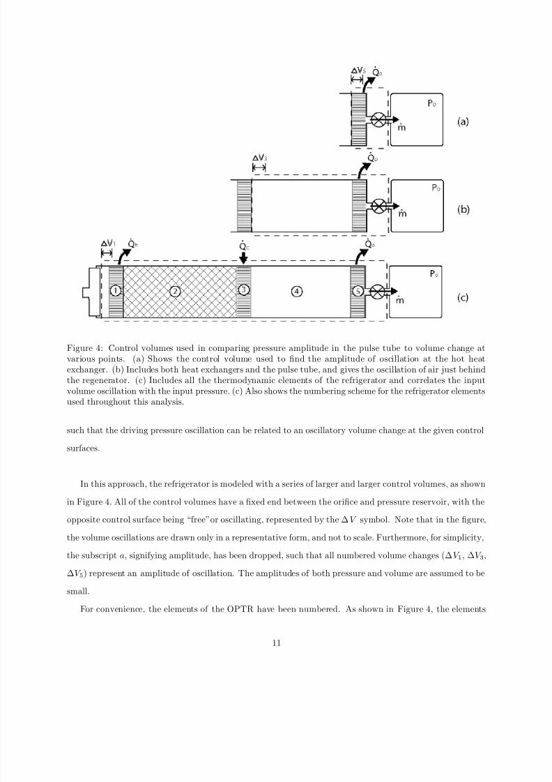
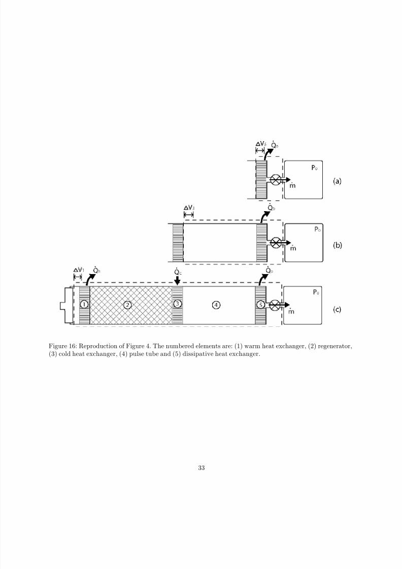
Figure 4: Control volumes used in comparing pressure amplitude in the pulse tube to volume change atvarious points. (a) Shows the control volume used to nd the amplitude of oscillation at the hot heatexchanger. (b) Includes both heat exchangers and the pulse tube, and gives the oscillation of air just behindthe regenerator. (c) Includes all the thermodynamic elements of the refrigerator and correlates the inputvolume oscillation with the input pressure. (c) Also shows the numbering scheme for the refrigerator elementsused throughout this analysis.

such that the driving pressure oscillation can be related to an oscillatory volume change at the given control

surfaces.

In this approach, the refrigerator is modeled with a series of larger and larger control volumes, as shown

in Figure 4. All of the control volumes have a xed end between the orice and pressure reservoir, with the

opposite control surface being “free”or oscillating, represented by the ∆ V symbol. Note that in the gure,

the volume oscillations are drawn only in a representative form, and not to scale. Furthermore, for simplicity,

the subscript a, signifying amplitude, has been dropped, such that all numbered volume changes (∆ V 1 , ∆ V 3 ,

∆ V 5) represent an amplitude of oscillation. The amplitudes of both pressure and volume are assumed to be

small.

For convenience, the elements of the OPTR have been numbered. As shown in Figure 4, the elements

11



are: (1) warm heat exchanger, (2) regenerator, (3) cold heat exchanger, (4) pulse tube and (5) dissipative

heat exchanger. Figure 4 also shows that all of the oscillating control surfaces are associated with the three

heat exchangers (and are labeled correspondingly: ∆ V 1 , ∆ V 3 , ∆ V 5). The reasoning for this is described in

the preceding explanation of cooling power.

As described above, the cold heat exchanger is modeled as having varying volume to account for the work

transfer from the moving displacement gas. Similarly, the warm end of the pulse tube must also be modeled

in the same way, since the heat rejection occurs at the hot end via compression. Also, as with the cold heat

exchanger, this heat exchanger is taken to be at a constant temperature ( T h ). Thus, the displacement of the

gas in the pulse tube is accounted for by ∆ V 3 and ∆ V 5 . The heat exchanger prior to the regenerator is also

modeled as isothermal and with oscillating volume, since it is assumed that the compression work from the

pressurized input uid is transferred here.

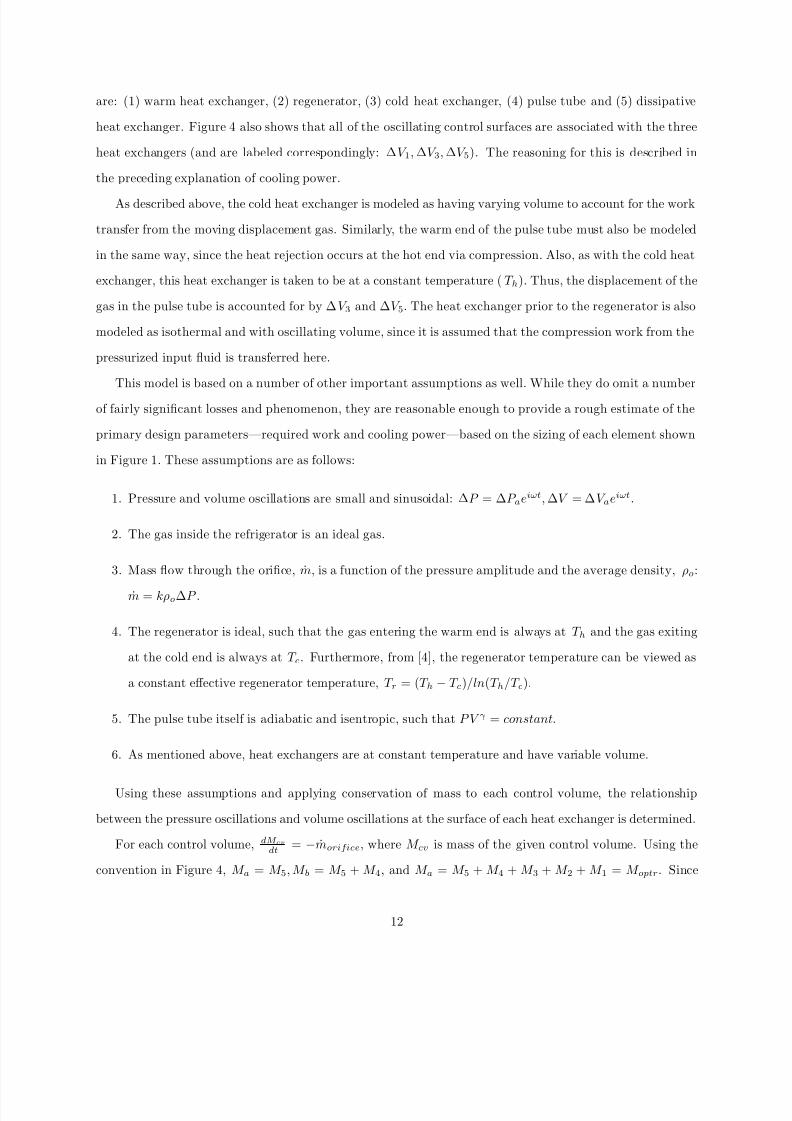
This model is based on a number of other important assumptions as well. While they do omit a number

of fairly signicant losses and phenomenon, they are reasonable enough to provide a rough estimate of the

primary design parameters required work and cooling power based on the sizing of each element shown

in Figure 1. These assumptions are as follows:

1. Pressure and volume oscillations are small and sinusoidal: ∆ P = ∆ P a eiωt , ∆ V = ∆ V a eiωt .

2. The gas inside the refrigerator is an ideal gas.

3. Mass ow through the orice, m , is a function of the pressure amplitude and the average density, ρo :

m = kρo ∆ P .

4. The regenerator is ideal, such that the gas entering the warm end is always at T h and the gas exiting

at the cold end is always at T c . Furthermore, from [4], the regenerator temperature can be viewed as

a constant effective regenerator temperature, T r = ( T h − T c )/ln (T h /T c ).

5. The pulse tube itself is adiabatic and isentropic, such that P V γ = constant .

6. As mentioned above, heat exchangers are at constant temperature and have variable volume.

Using these assumptions and applying conservation of mass to each control volume, the relationship

between the pressure oscillations and volume oscillations at the surface of each heat exchanger is determined.

For each control volume, dM cvdt = − m orifice , where M cv is mass of the given control volume. Using the

convention in Figure 4, M a = M 5 , M b = M 5 + M 4 , and M a = M 5 + M 4 + M 3 + M 2 + M 1 = M optr . Since

12



the gas inside the OPTR is taken to be ideal and the temperature of element 1, 2, 3, and 5 are taken to

be constant (using the effective regenerator temperature T r ), the mass of each of these elements can be

expressed as M i = P V i /RT i , where i is the element index (as dened in Figure 4), P is the time-varying

pressure within the element, V is the time-varying volume, R is the ideal gas constant (mass basis) and T

is the temperature of the element. The pulse tube mass, however, must be expressed using the denition

M 4 = V 4(ρ), since temperature is not uniform.

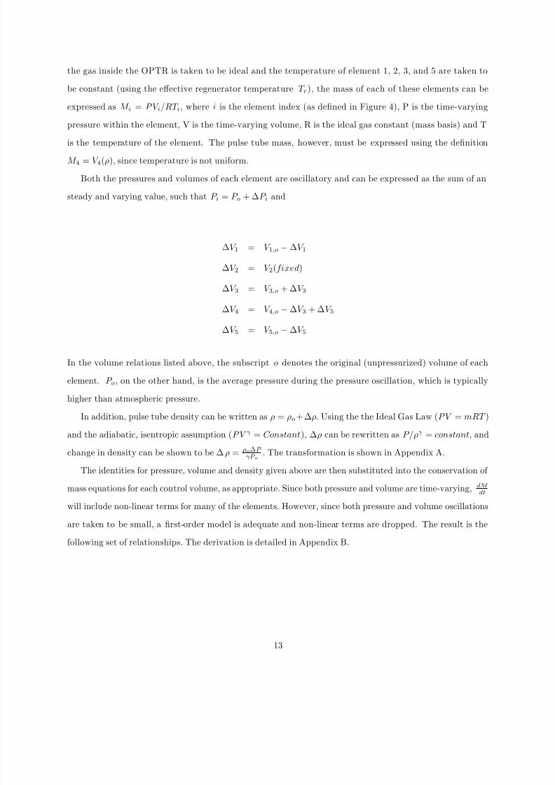
Both the pressures and volumes of each element are oscillatory and can be expressed as the sum of an

steady and varying value, such that P i = P o + ∆ P i and

∆ V 1 = V 1,o − ∆ V 1

∆ V 2 = V 2(fixed )

∆ V 3 = V 3,o + ∆ V 3

∆ V 4 = V 4,o − ∆ V 3 + ∆ V 5

∆ V 5 = V 5,o − ∆ V 5

In the volume relations listed above, the subscript o denotes the original (unpressurized) volume of each

element. P o , on the other hand, is the average pressure during the pressure oscillation, which is typically

higher than atmospheric pressure.

In addition, pulse tube density can be written as ρ = ρo +∆ ρ. Using the the Ideal Gas Law ( P V = mRT )

and the adiabatic, isentropic assumption ( P V γ = Constant ), ∆ ρ can be rewritten as P/ρ γ = constant , and

change in density can be shown to be ∆ ρ = ρ o ∆ P γP o

. The transformation is shown in Appendix A.

The identities for pressure, volume and density given above are then substituted into the conservation of

mass equations for each control volume, as appropriate. Since both pressure and volume are time-varying, dM dt

will include non-linear terms for many of the elements. However, since both pressure and volume oscillations

are taken to be small, a rst-order model is adequate and non-linear terms are dropped. The result is the

following set of relationships. The derivation is detailed in Appendix B.

13



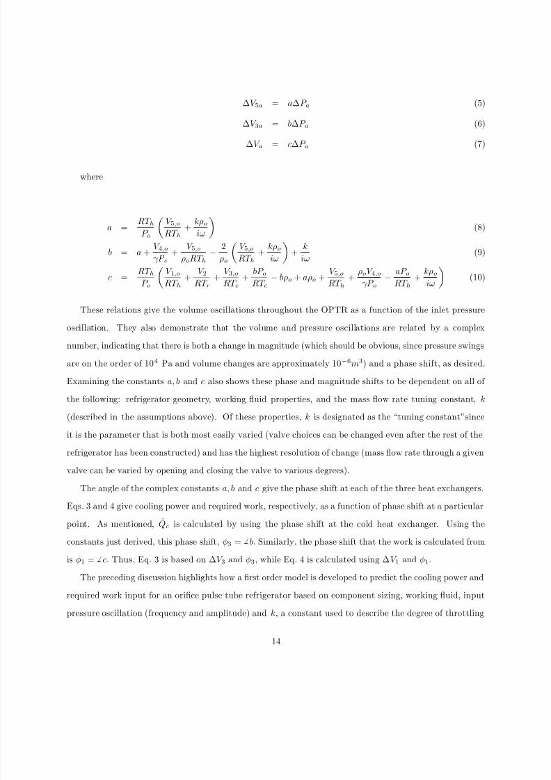
∆ V 5a = a∆ P a (5)

∆ V 3a = b∆ P a (6)

∆ V a = c∆ P a (7)

where

a =RT hP o

V 5,o

RT h+

kρo

iω(8)

b = a +V 4,o

γP o+

V 5,o

ρo RT h−

2ρo

V 5 ,o

RT h+

kρo

iω+

kiω

(9)

c = RT hP o

V 1,oRT h

+ V 2RT r

+ V 3 ,oRT c

+ bP oRT c

− bρo + aρ o + V 5 ,oRT h

+ ρo V 4,oγP o

− aP oRT h

+ kρoiω

(10)

These relations give the volume oscillations throughout the OPTR as a function of the inlet pressure

oscillation. They also demonstrate that the volume and pressure oscillations are related by a complex

number, indicating that there is both a change in magnitude (which should be obvious, since pressure swings

are on the order of 10 4 Pa and volume changes are approximately 10 − 6m3) and a phase shift, as desired.

Examining the constants a, b and c also shows these phase and magnitude shifts to be dependent on all of

the following: refrigerator geometry, working uid properties, and the mass ow rate tuning constant, k

(described in the assumptions above). Of these properties, k is designated as the “tuning constant”since

it is the parameter that is both most easily varied (valve choices can be changed even after the rest of the

refrigerator has been constructed) and has the highest resolution of change (mass ow rate through a given

valve can be varied by opening and closing the valve to various degrees).

The angle of the complex constants a, b and c give the phase shift at each of the three heat exchangers.

Eqs. 3 and 4 give cooling power and required work, respectively, as a function of phase shift at a particular

point. As mentioned, Qc is calculated by using the phase shift at the cold heat exchanger. Using the

constants just derived, this phase shift, φ3

= b. Similarly, the phase shift that the work is calculated from

is φ1 = c. Thus, Eq. 3 is based on ∆ V 3 and φ3 , while Eq. 4 is calculated using ∆ V 1 and φ1 .

The preceding discussion highlights how a rst order model is developed to predict the cooling power and

required work input for an orice pulse tube refrigerator based on component sizing, working uid, input

pressure oscillation (frequency and amplitude) and k, a constant used to describe the degree of throttling

14



between the pulse tube and pressure reservoir. In using this model to design an OPTR, sizing and working

uid can be taken to be limited by “external ”constraints desired overall size and gas availability such

that k, pressure amplitude, and frequency of oscillation are the variables that can be easily manipulated,

after the pulse tube has been constructed to give a desired cooling power and temperature difference.

2.2 Limitations of the Model

This model of an orice pulse tube refrigerator makes a number of gross assumptions that limit its accuracy

in predicting cooling power. The largest source of error in this model is the assumption of essentially no

losses. In making this assumption, entropy generation in all components (with the exception of the throttle,

which is inherently lossy), is taken to be zero. However, friction losses, imperfect thermal recovery within the

regenerator and unintentional heat transfer into and out of other metal elements, such as the valve manifold

or pressure reservoir, will also contribute losses not included in the model. In addition, the heat exchangershave been assumed to be isothermal and the regenerator is characterized by a known temperature gradient,

which are simplications of the actual thermal behavior.

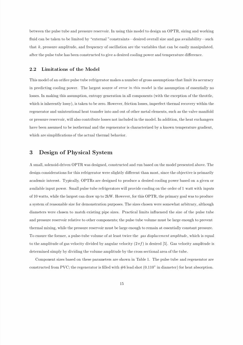
3 Design of Physical System

A small, solenoid-driven OPTR was designed, constructed and run based on the model presented above. The

design considerations for this refrigerator were slightly different than most, since the objective is primarily

academic interest. Typically, OPTRs are designed to produce a desired cooling power based on a given oravailable input power. Small pulse tube refrigerators will provide cooling on the order of 1 watt with inputs

of 10 watts, while the largest can draw up to 2kW. However, for this OPTR, the primary goal was to produce

a system of reasonable size for demonstration purposes. The sizes chosen were somewhat arbitrary, although

diameters were chosen to match existing pipe sizes. Practical limits inuenced the size of the pulse tube

and pressure reservoir relative to other components; the pulse tube volume must be large enough to prevent

thermal mixing, while the pressure reservoir must be large enough to remain at essentially constant pressure.

To ensure the former, a pulse-tube volume of at least twice the gas displacement amplitude , which is equal

to the amplitude of gas velocity divided by angular velocity (2 πf ) is desired [5]. Gas velocity amplitude is

determined simply by dividing the volume amplitude by the cross sectional area of the tube.

Component sizes based on these parameters are shown in Table 1. The pulse tube and regenerator are

constructed from PVC; the regenerator is lled with #6 lead shot (0.110” in diameter) for heat absorption.

15



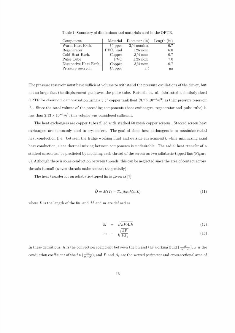
Table 1: Summary of dimensions and materials used in the OPTR.

Component Material Diameter (in) Length (in)Warm Heat Exch. Copper 3/4 nominal 0.7Regenerator PVC, lead 1.25 nom. 6.0Cold Heat Exch. Copper 3/4 nom. 0.7Pulse Tube PVC 1.25 nom. 7.0Dissipative Heat Exch. Copper 3/4 nom. 0.7Pressure reservoir Copper 3.5 na

The pressure reservoir must have sufficient volume to withstand the pressure oscillations of the driver, but

not so large that the displacement gas leaves the pulse tube. Rotundo et. al. fabricated a similarly sized

OPTR for classroom demonstration using a 3.5” copper tank oat (3 .7 × 10− 4m3) as their pressure reservoir

[6]. Since the total volume of the preceding components (heat exchangers, regenerator and pulse tube) is

less than 2 .13 × 10− 4

m3

, this volume was considered sufficient.The heat exchangers are copper tubes lled with stacked 50 mesh copper screens. Stacked screen heat

exchangers are commonly used in cryocoolers. The goal of these heat exchangers is to maximize radial

heat conduction (i.e. between the fridge working uid and outside environment), while minimizing axial

heat conduction, since thermal mixing between components is undesirable. The radial heat transfer of a

stacked screen can be predicted by modeling each thread of the screen as two adiabatic-tipped ns (Figure

5). Although there is some conduction between threads, this can be neglected since the area of contact across

threads is small (woven threads make contact tangentially).

The heat transfer for an adiabatic-tipped n is given as [7]:

Q = M (T b − T ∞ )tanh (mL ) (11)

where L is the length of the n, and M and m are dened as

M =

hP A c k (12)

m = hP kAc (13)

In these denitions, h is the convection coefficient between the n and the working uid ( W m 2 − K ), k is the

conduction coefficient of the n ( W m − K ), and P and Ac are the wetted perimeter and cross-sectional area of

16



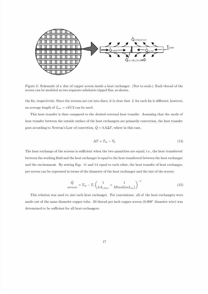
Figure 5: Schematic of a disc of copper screen inside a heat exchanger. (Not to scale.) Each thread of thescreen can be modeled as two separate adiabatic-tipped ns, as shown.

the n, respectively. Since the screens are cut into discs, it is clear that L for each n is different; however,

an average length of Lav = πD/ 2 can be used.

This heat transfer is then compared to the desired external heat transfer. Assuming that the mode of

heat transfer between the outside surface of the heat exchangers are primarily convection, the heat transfer

goes according to Newton’s Law of convection, Q = hA∆ T , where in this case,

∆ T = T ∞ − T b (14)

The heat exchange of the screens is sufficient when the two quantities are equal; i.e., the heat transferred

between the working uid and the heat exchanger is equal to the heat transferred between the heat exchanger

and the environment. By setting Eqs. 11 and 14 equal to each other, the heat transfer of heat exchanger,

per screen can be expressed in terms of the diameter of the heat exchanger and the size of the screen:

Qscreen

= T ∞ − T c1

hA c,hex+

1Mtanh (mL av )

− 1

(15)

This relation was used to size each heat exchanger. For convenience, all of the heat exchangers were

made out of the same diameter copper tube. 50 thread per inch copper screen (0.009” diameter wire) was

determined to be sufficient for all heat exchangers.

17



3.1 Fabrication

As mentioned, standard pipe diameters were used to simplify the fabrication process. Each component was

cut from pipe of appropriate material to the length specied above. The pulse tube, simply an open tube,

was cut out of 3/4” PVC pipe and required no further modication. To join the copper heat exchangers to

each end of the pulse tube, the ends were turned to the diameter of the cooper tube, approximately 0.25”

deep. The regenerator was cut to length out of 1.25” PVC pipe and lled with #6 (0.110” diameter) lead

shot. Appropriately sized end caps were used to connect mating parts as with the pulse tube. Two layers

of woven copper screen (50 mesh) were edge epoxied to each end in order to retain the lead shot within

the regenerator. Note that in order to maximize entropy transfer, the heat exchangers on either end of the

regenerator should be in direct contact with the end of the regenerator. Thus, additional retaining screens

were affixed to the end cap and the both caps were lled with lead shot.

Both the hot and cold heat exchangers were fabricated from 3/4” (nominal) copper pipe. In order toimprove heat exchange between the owing gas inside and the ambient environment, 50 mesh copper screens

were soldered into the tubes, as noted above. The screens were cut to have a slight interference t with the

inner diameter of the copper tube using a specially fabricated steel punch. Twenty screens were placed in

each heat exchanger in order to maximize heat transfer while still having a reasonable pressure drop. Each

screen was spaced out using a ring of copper wire to ensure even heat exchange throughout the entire length

of the heat exchanger.

The screens were then soldered into the copper tubes. The interference t of the screens not only ensured

adequate heat exchange but also helped the soldering processes. Instead of xing each screen individually,

all of the screens were soldered at once. This was done by pre-coating the interior of a copper tube with

lead-tin solder and ux, and then inserting an entire stack of screens and spacers into the tube. The tube was

then heated, and additional solder was owed onto the end screens to ensure a strong bond. A completed

heat exchanger is shown in Figure 6.

The pressure reservoir was simply a 3.5” diameter, 1/8” NPT copper tank oat, drilled through the

threaded connection to allow gas to ow into the hollow sphere. The tank oat was chosen based on the

suggestion of [6] for its sufficient volume and its ease in connection with the orice valve, to be discussed

below.

Throttling between the pulse tube and the pressure reservoir was achieved with a standard needle valve.

The required ow rate through the valve was determined by the model by calculating the volume ow rate

out of the hot heat exchanger (∆ V 5), as described in Sec. 2. For needle valves, ow rate is related to the

18



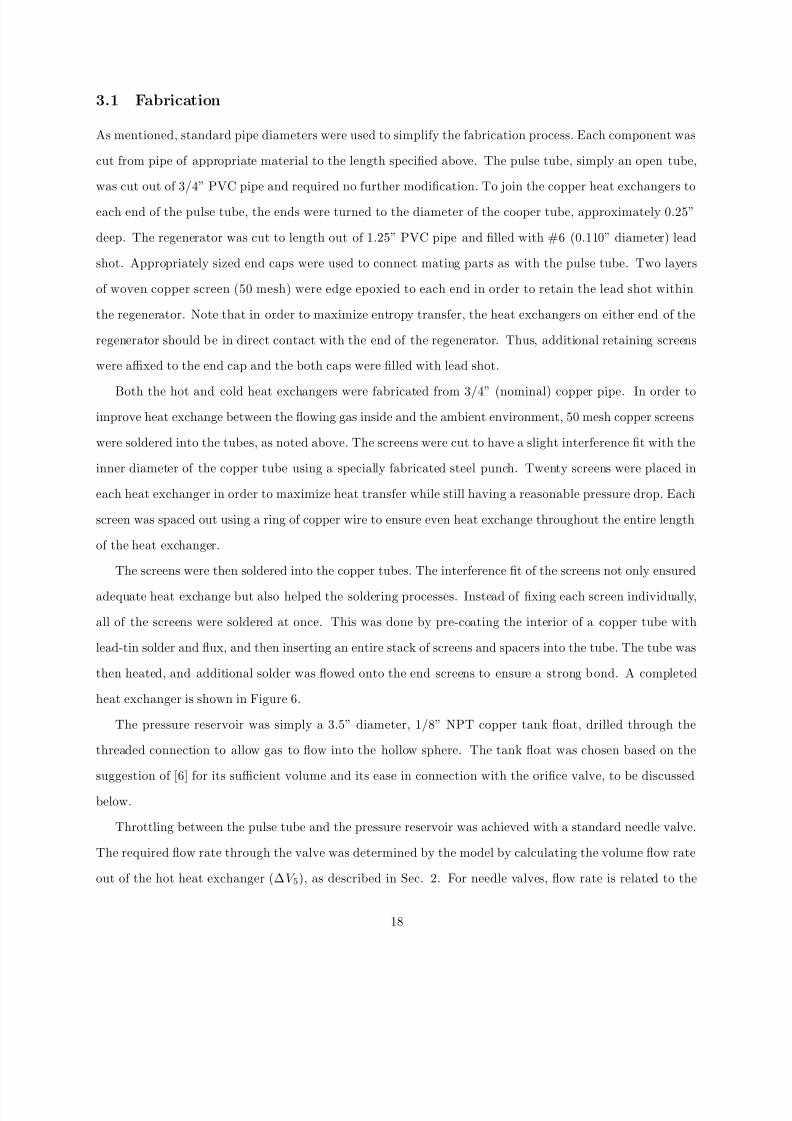
Figure 6: Heat exchangers used in this OPTR. 50 mesh copper screens were cut and soldered into 3/4”nominal copper pipe. Each heat exchanger contains 20 screens spaced with 20 gauge copper wire.

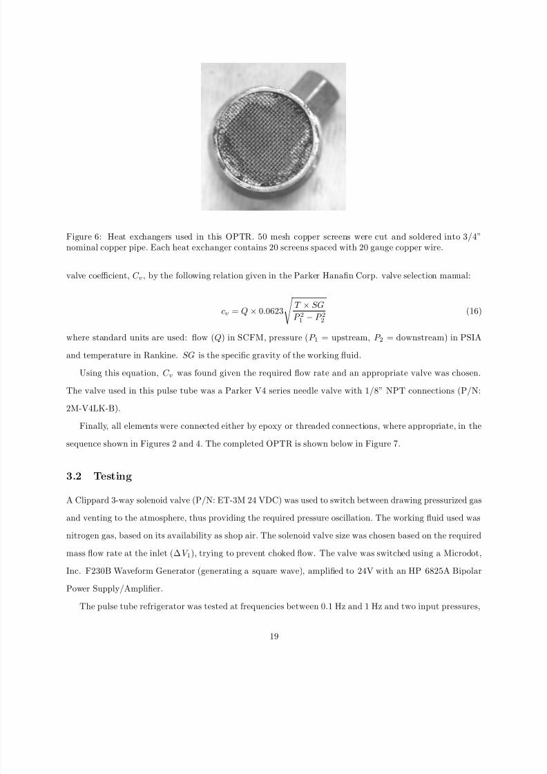
valve coefficient, C v , by the following relation given in the Parker Hanan Corp. valve selection manual:

cv = Q × 0.0623 T × SGP 21 − P 22

(16)

where standard units are used: ow ( Q) in SCFM, pressure ( P 1 = upstream, P 2 = downstream) in PSIA

and temperature in Rankine. SG is the specic gravity of the working uid.

Using this equation, C v was found given the required ow rate and an appropriate valve was chosen.

The valve used in this pulse tube was a Parker V4 series needle valve with 1/8” NPT connections (P/N:

2M-V4LK-B).

Finally, all elements were connected either by epoxy or threaded connections, where appropriate, in the

sequence shown in Figures 2 and 4. The completed OPTR is shown below in Figure 7.

3.2 Testing

A Clippard 3-way solenoid valve (P/N: ET-3M 24 VDC) was used to switch between drawing pressurized gas

and venting to the atmosphere, thus providing the required pressure oscillation. The working uid used was

nitrogen gas, based on its availability as shop air. The solenoid valve size was chosen based on the required

mass ow rate at the inlet (∆ V 1), trying to prevent choked ow. The valve was switched using a Microdot,

Inc. F230B Waveform Generator (generating a square wave), amplied to 24V with an HP 6825A Bipolar

Power Supply/Amplier.

The pulse tube refrigerator was tested at frequencies between 0.1 Hz and 1 Hz and two input pressures,

19



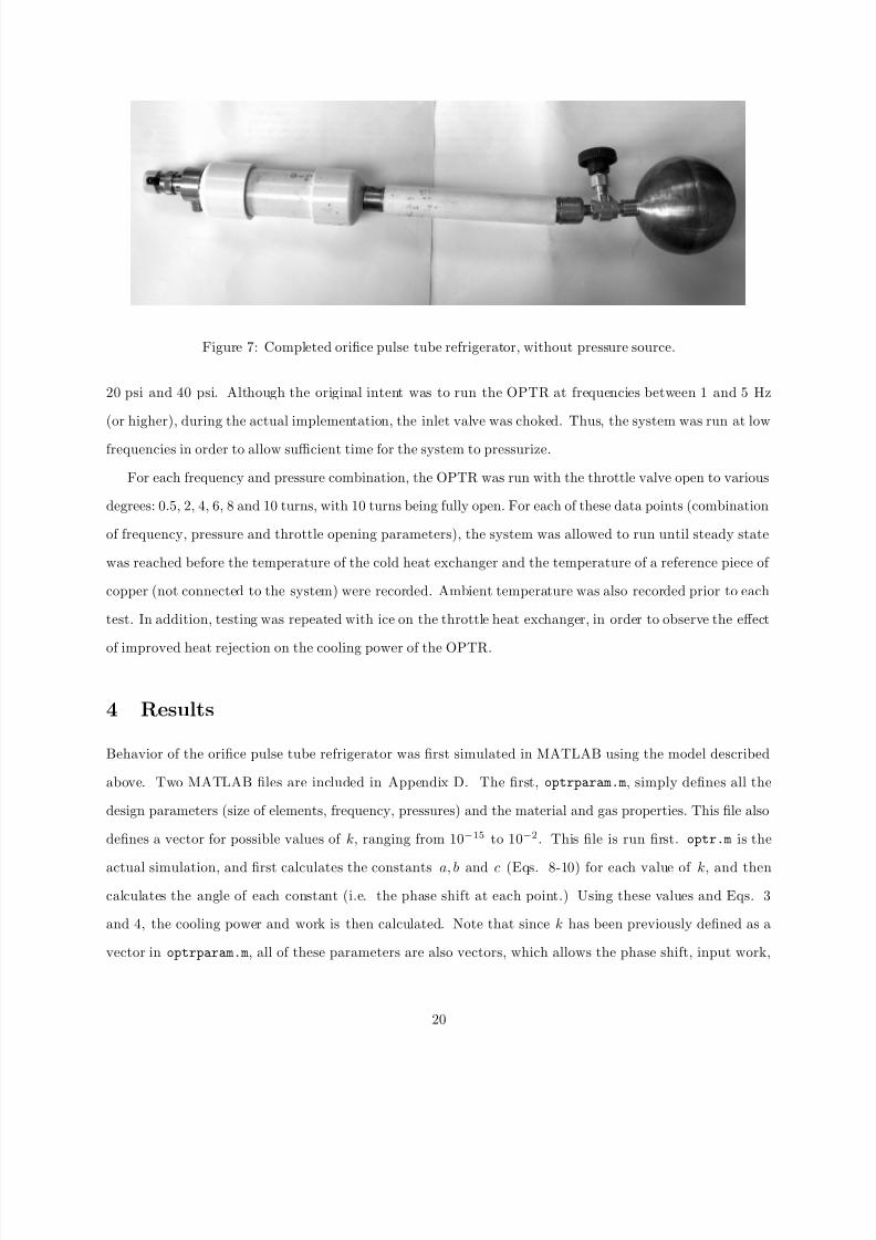
Figure 7: Completed orice pulse tube refrigerator, without pressure source.

20 psi and 40 psi. Although the original intent was to run the OPTR at frequencies between 1 and 5 Hz

(or higher), during the actual implementation, the inlet valve was choked. Thus, the system was run at low

frequencies in order to allow sufficient time for the system to pressurize.

For each frequency and pressure combination, the OPTR was run with the throttle valve open to various

degrees: 0.5, 2, 4, 6, 8 and 10 turns, with 10 turns being fully open. For each of these data points (combination

of frequency, pressure and throttle opening parameters), the system was allowed to run until steady state

was reached before the temperature of the cold heat exchanger and the temperature of a reference piece of

copper (not connected to the system) were recorded. Ambient temperature was also recorded prior to each

test. In addition, testing was repeated with ice on the throttle heat exchanger, in order to observe the effect

of improved heat rejection on the cooling power of the OPTR.

4 Results

Behavior of the orice pulse tube refrigerator was rst simulated in MATLAB using the model described

above. Two MATLAB les are included in Appendix D. The rst, optrparam.m , simply denes all the

design parameters (size of elements, frequency, pressures) and the material and gas properties. This le also

denes a vector for possible values of k, ranging from 10 − 15 to 10− 2 . This le is run rst. optr.m is the

actual simulation, and rst calculates the constants a, b and c (Eqs. 8-10) for each value of k, and thencalculates the angle of each constant (i.e. the phase shift at each point.) Using these values and Eqs. 3

and 4, the cooling power and work is then calculated. Note that since k has been previously dened as a

vector in optrparam.m , all of these parameters are also vectors, which allows the phase shift, input work,

20



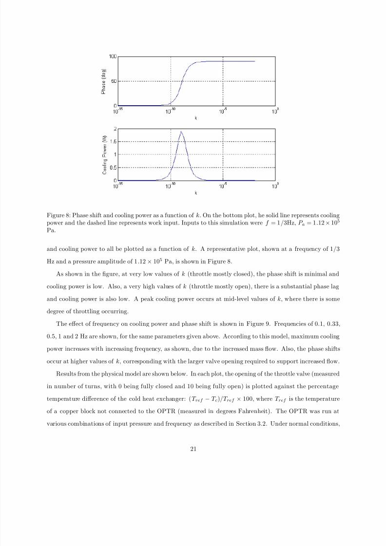
Figure 8: Phase shift and cooling power as a function of k. On the bottom plot, he solid line represents coolingpower and the dashed line represents work input. Inputs to this simulation were f = 1 / 3Hz, P a = 1 .12 × 105

Pa.

and cooling power to all be plotted as a function of k. A representative plot, shown at a frequency of 1/3

Hz and a pressure amplitude of 1 .12 × 105 Pa, is shown in Figure 8.

As shown in the gure, at very low values of k (throttle mostly closed), the phase shift is minimal and

cooling power is low. Also, a very high values of k (throttle mostly open), there is a substantial phase lagand cooling power is also low. A peak cooling power occurs at mid-level values of k, where there is some

degree of throttling occurring.

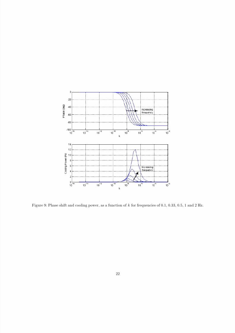
The effect of frequency on cooling power and phase shift is shown in Figure 9. Frequencies of 0.1, 0.33,

0.5, 1 and 2 Hz are shown, for the same parameters given above. According to this model, maximum cooling

power increases with increasing frequency, as shown, due to the increased mass ow. Also, the phase shifts

occur at higher values of k, corresponding with the larger valve opening required to support increased ow.

Results from the physical model are shown below. In each plot, the opening of the throttle valve (measured

in number of turns, with 0 being fully closed and 10 being fully open) is plotted against the percentage

temperature difference of the cold heat exchanger: ( T ref − T c )/T ref × 100, where T ref is the temperature

of a copper block not connected to the OPTR (measured in degrees Fahrenheit). The OPTR was run at

various combinations of input pressure and frequency as described in Section 3.2. Under normal conditions,

21



Figure 9: Phase shift and cooling power, as a function of k for frequencies of 0.1, 0.33, 0.5, 1 and 2 Hz.

22



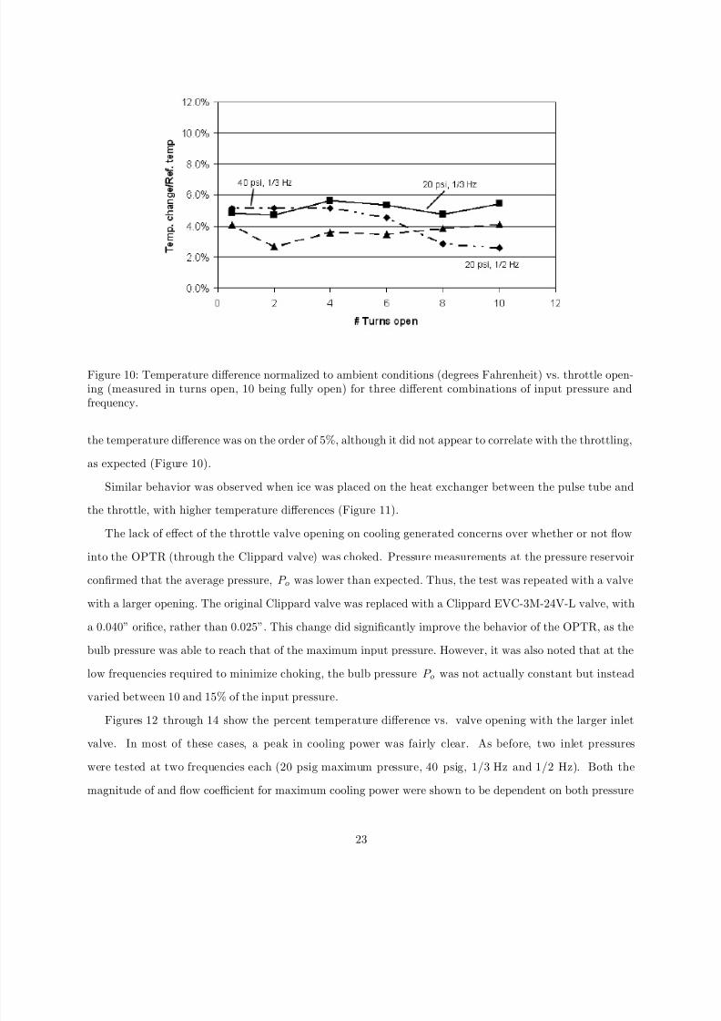
Figure 10: Temperature difference normalized to ambient conditions (degrees Fahrenheit) vs. throttle open-ing (measured in turns open, 10 being fully open) for three different combinations of input pressure andfrequency.

the temperature difference was on the order of 5%, although it did not appear to correlate with the throttling,

as expected (Figure 10).

Similar behavior was observed when ice was placed on the heat exchanger between the pulse tube and

the throttle, with higher temperature differences (Figure 11).

The lack of effect of the throttle valve opening on cooling generated concerns over whether or not owinto the OPTR (through the Clippard valve) was choked. Pressure measurements at the pressure reservoir

conrmed that the average pressure, P o was lower than expected. Thus, the test was repeated with a valve

with a larger opening. The original Clippard valve was replaced with a Clippard EVC-3M-24V-L valve, with

a 0.040” orice, rather than 0.025”. This change did signicantly improve the behavior of the OPTR, as the

bulb pressure was able to reach that of the maximum input pressure. However, it was also noted that at the

low frequencies required to minimize choking, the bulb pressure P o was not actually constant but instead

varied between 10 and 15% of the input pressure.

Figures 12 through 14 show the percent temperature difference vs. valve opening with the larger inlet

valve. In most of these cases, a peak in cooling power was fairly clear. As before, two inlet pressures

were tested at two frequencies each (20 psig maximum pressure, 40 psig, 1/3 Hz and 1/2 Hz). Both the

magnitude of and ow coefficient for maximum cooling power were shown to be dependent on both pressure

23



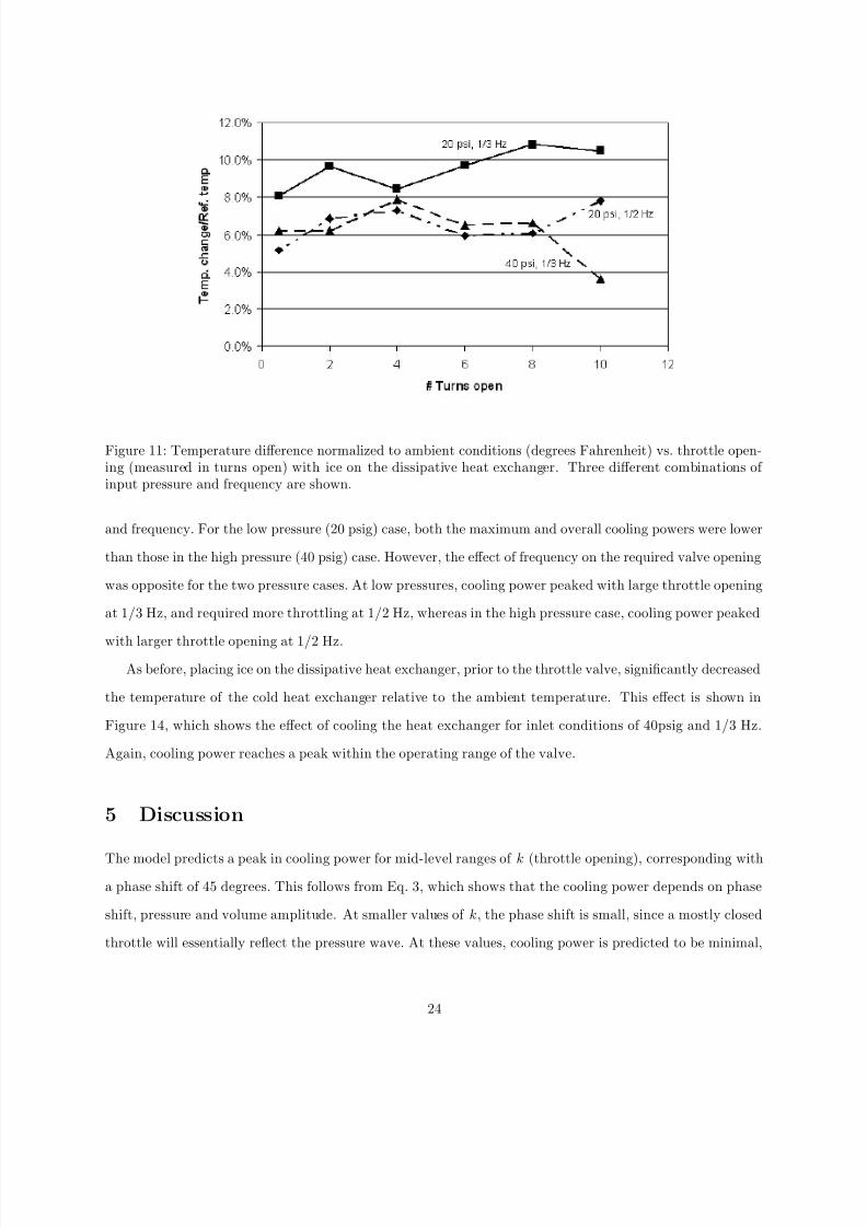
Figure 11: Temperature difference normalized to ambient conditions (degrees Fahrenheit) vs. throttle open-ing (measured in turns open) with ice on the dissipative heat exchanger. Three different combinations of input pressure and frequency are shown.

and frequency. For the low pressure (20 psig) case, both the maximum and overall cooling powers were lower

than those in the high pressure (40 psig) case. However, the effect of frequency on the required valve opening

was opposite for the two pressure cases. At low pressures, cooling power peaked with large throttle opening

at 1/3 Hz, and required more throttling at 1/2 Hz, whereas in the high pressure case, cooling power peaked

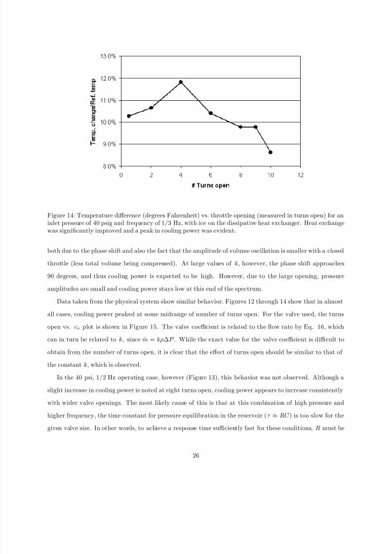
with larger throttle opening at 1/2 Hz.As before, placing ice on the dissipative heat exchanger, prior to the throttle valve, signicantly decreased

the temperature of the cold heat exchanger relative to the ambient temperature. This effect is shown in

Figure 14, which shows the effect of cooling the heat exchanger for inlet conditions of 40psig and 1/3 Hz.

Again, cooling power reaches a peak within the operating range of the valve.

5 Discussion

The model predicts a peak in cooling power for mid-level ranges of k (throttle opening), corresponding witha phase shift of 45 degrees. This follows from Eq. 3, which shows that the cooling power depends on phase

shift, pressure and volume amplitude. At smaller values of k, the phase shift is small, since a mostly closed

throttle will essentially reect the pressure wave. At these values, cooling power is predicted to be minimal,

24



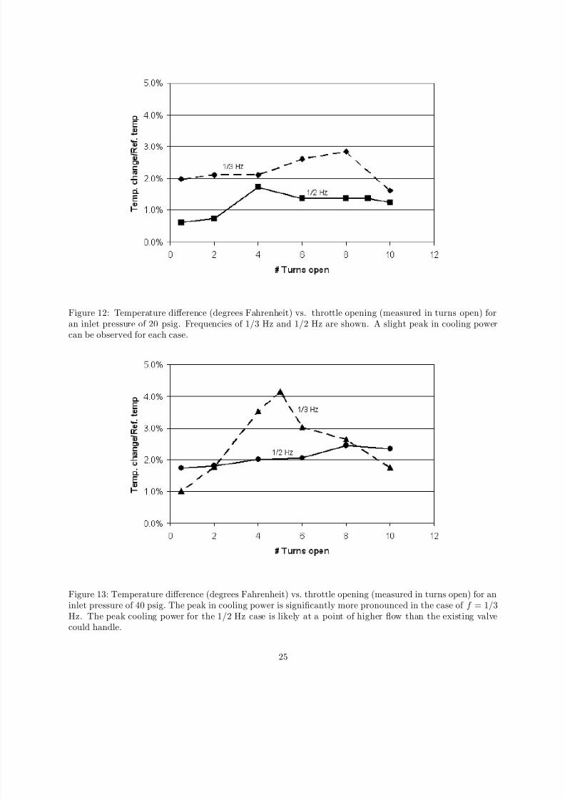
Figure 12: Temperature difference (degrees Fahrenheit) vs. throttle opening (measured in turns open) foran inlet pressure of 20 psig. Frequencies of 1/3 Hz and 1/2 Hz are shown. A slight peak in cooling powercan be observed for each case.

Figure 13: Temperature difference (degrees Fahrenheit) vs. throttle opening (measured in turns open) for aninlet pressure of 40 psig. The peak in cooling power is signicantly more pronounced in the case of f = 1 / 3Hz. The peak cooling power for the 1/2 Hz case is likely at a point of higher ow than the existing valvecould handle.

25



Figure 14: Temperature difference (degrees Fahrenheit) vs. throttle opening (measured in turns open) for aninlet pressure of 40 psig and frequency of 1/3 Hz, with ice on the dissipative heat exchanger. Heat exchangewas signicantly improved and a peak in cooling power was evident.

both due to the phase shift and also the fact that the amplitude of volume oscillation is smaller with a closed

throttle (less total volume being compressed). At large values of k, however, the phase shift approaches

90 degrees, and thus cooling power is expected to be high. However, due to the large opening, pressure

amplitudes are small and cooling power stays low at this end of the spectrum.Data taken from the physical system show similar behavior. Figures 12 through 14 show that in almost

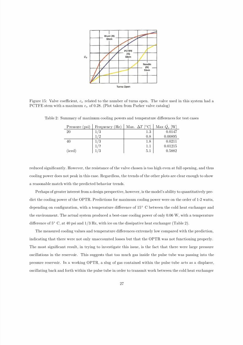
all cases, cooling power peaked at some midrange of number of turns open. For the valve used, the turns

open vs. cv plot is shown in Figure 15. The valve coefficient is related to the ow rate by Eq. 16, which

can in turn be related to k, since m = kρ∆ P . While the exact value for the valve coefficient is difficult to

obtain from the number of turns open, it is clear that the effect of turns open should be similar to that of

the constant k, which is observed.

In the 40 psi, 1/2 Hz operating case, however (Figure 13), this behavior was not observed. Although a

slight increase in cooling power is noted at eight turns open, cooling power appears to increase consistently

with wider valve openings. The most likely cause of this is that at this combination of high pressure and

higher frequency, the time constant for pressure equilibration in the reservoir ( τ ≈ RC ) is too slow for the

given valve size. In other words, to achieve a response time sufficiently fast for these conditions, R must be

26



Figure 15: Valve coefficient, cv related to the number of turns open. The valve used in this system had aPCTFE stem with a maximum cv of 0.28. (Plot taken from Parker valve catalog)

Table 2: Summary of maximum cooling powers and temperature differences for test cases

Pressure (psi) Frequency (Hz) Max. ∆ T [◦ C] Max Qc [W]20 1/3 1.3 0.0147

1/2 0.8 0.0089540 1/3 1.8 0.0211

1/2 1.1 0.01215(iced) 1/3 5.1 0.5882

reduced signicantly. However, the resistance of the valve chosen is too high even at full opening, and thus

cooling power does not peak in this case. Regardless, the trends of the other plots are clear enough to show

a reasonable match with the predicted behavior trends.

Perhaps of greater interest from a design perspective, however, is the model’s ability to quantitatively pre-

dict the cooling power of the OPTR. Predictions for maximum cooling power were on the order of 1-2 watts,

depending on conguration, with a temperature difference of 15 ◦ C between the cold heat exchanger and

the environment. The actual system produced a best-case cooling power of only 0.06 W, with a temperature

difference of 5◦ C, at 40 psi and 1/3 Hz, with ice on the dissipative heat exchanger (Table 2).

The measured cooling values and temperature differences extremely low compared with the prediction,

indicating that there were not only unaccounted losses but that the OPTR was not functioning properly.

The most signicant result, in trying to investigate this issue, is the fact that there were large pressure

oscillations in the reservoir. This suggests that too much gas inside the pulse tube was passing into the

pressure reservoir. In a working OPTR, a slug of gas contained within the pulse tube acts as a displacer,

oscillating back and forth within the pulse tube in order to transmit work between the cold heat exchanger

27



and the heat exchanger at the throttle. Also, containing this displacement gas entirely within the pulse tube

ensures insulation between the two heat exchangers. If the volume oscillations are too large, the gas slug

will pass completely through the pulse tube and the OPTR will lose its cooling ability as warm gas from the

throttle will be actively mixed with the gas in the cold heat exchanger.

A rough conservation of mass calculation veries this phenomenon. Assuming the pressure reservoir to be

roughly constant temperature, that fact that P o is not constant indicates that the mass inside the reservoir

is changing ( P V = mRT ). In addition, any additional mass entering the reservoir must come from the

pulse tube, i.e. |∆ m pt | = |∆ m res | . Using the ideal gas law to express mass in terms of other properties

and assuming (conservatively) that the reservoir temperature and pulse temperature are both constant and

equal, we have that

P av (∆ V pt + V res ) = (∆ P + P av )V res , (17)

where P av is the average pressure in the pulse tube and OPTR, ∆ V pt is instantaneous volume of the displacing

gas within the pulse tube, and V res is the xed reservoir volume. The volume of gas within the pulse tube is

related to the length of the displacing gas easily by geometry, V pt = L(πD 2pt / 4). Substituting and rearranging,

the length of travel, L of the displacing gas is expressed as

L =∆ P

P av V res

4πD 2

pt(18)

This length must be signicantly shorter than the length of the pulse tube. Using various measuredreservoir pressure changes, L was found to vary between 8.0 cm and 15.2 cm. The pulse tube, however,

is 7”(17.8 cm) long, and therefore a signicant amount of the displacing gas that is escaping through the

throttle valve. The measurable but not extreme change in cold temperature when ice was placed near the

throttle is consistent this theory. Given these travel lengths, it is likely that the ice cooled a section of gas

that was carried down the length of the pulse tube far enough that it mixed with the gas in the cold heat

exchanger.

Increasing the length of the pulse tube or decreasing reservoir size would also shorten the travel length

of the gas slug. Practically speaking, however, the pulse tube would have to be extraordinarily long to offset

the large pressure deviations in the reservoir and decreasing the volume of the reservoir would itself make the

reservoir more prone to pressure changes. From Eq. 18, and choosing a reasonable L to be approximately 1

cm, the maximum tolerable pressure change in the reservoir is about 0.1% of the input pressure. This could

28



be achieved with increased throttling or faster driving frequencies, although as mentioned before, increased

input frequency presented additional problems.

6 Conclusion

A rst-order model for the behavior of an orice pulse tube refrigerator was developed and validated through

the construction of a physical refrigerator. At low driving frequencies the refrigerator was able to produce

some cooling, although the amount was substantially lower than predicted. The low cooling power was likely

a result of large volume oscillations within the pulse tube, causing thermal mixing between the warm and

cold ends of the pulse tube.

These large volume oscillations were caused by large pressure swings within the pressure reservoir (10-

15% of the inlet pressure), which were, in turn, a result of the low running frequencies required to prevent

ow choking at inlet of the OPTR. Greater throttling between the pulse tube and pressure reservoir would

also reduce these pressure swings. Thus, two major proposals for achieving the desired cooling power are

(1) increase the size of the inlet valve and run at higher frequencies and (2) increase throttling. A suggested

minimum input frequency is 2 Hz; although in this model, no cooling power was observed at this frequency,

testing did show the pressure reservoir to be roughly constant for these conditions.

The model presented above, then, is adequate for describing general behavior and trends in OPTR

operation, but overly simplied for actual design of pulse tube refrigerators. In particular, ow limitations

and warnings for pulse tube displacement distance are not included. These two factors proved to be the

most detrimental to the behavior of the OPTR. While these issues are likely correctly with modications

to the physical OPTR, from the perspective of using the model as a design tool, it would be useful to

modify the code to ag these problems. Nevertheless, the current model is useful for preliminary sizing and

rst-order calculations, with the understanding that there exist some known potential problems and that

troubleshooting and modications would be required to physically implement such a system.

29



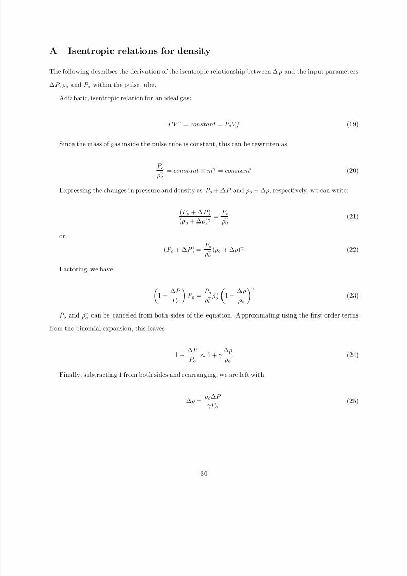
A Isentropic relations for density

The following describes the derivation of the isentropic relationship between ∆ ρ and the input parameters

∆ P, ρ o and P o within the pulse tube.

Adiabatic, isentropic relation for an ideal gas:

P V γ = constant = P o V γo (19)

Since the mass of gas inside the pulse tube is constant, this can be rewritten as

P oργ

o= constant × m γ = constant (20)

Expressing the changes in pressure and density as P o + ∆ P and ρo + ∆ ρ, respectively, we can write:

(P o + ∆ P )(ρo + ∆ ρ)γ =

P oργ

o(21)

or,

(P o + ∆ P ) =P oργ

o(ρo + ∆ ρ)γ (22)

Factoring, we have

1 +∆ P

P oP o =

P o

ργ

o

ργo 1 +

∆ ρ

ρo

γ

(23)

P o and ργo can be canceled from both sides of the equation. Approximating using the rst order terms

from the binomial expansion, this leaves

1 +∆ P P o

≈ 1 + γ ∆ ρρo

(24)

Finally, subtracting 1 from both sides and rearranging, we are left with

∆ ρ =ρo ∆ P γP o (25)

30



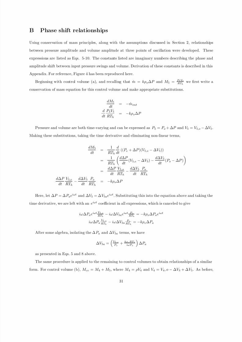
B Phase shift relationships

Using conservation of mass principles, along with the assumptions discussed in Section 2, relationships

between pressure amplitude and volume amplitude at three points of oscillation were developed. These

expressions are listed as Eqs. 5-10. The constants listed are imaginary numbers describing the phase andamplitude shift between input pressure swings and volume. Derivation of these constants is described in this

Appendix. For reference, Figure 4 has been reproduced here.

Beginning with control volume (a), and recalling that ˙ m = kρo ∆ P and M 5 = P 5 V 5RT h

we rst write a

conservation of mass equation for this control volume and make appropriate substitutions.

dM 5dt

= − m out

ddt

P 5V 5RT h

= − kρo ∆ P

Pressure and volume are both time-varying and can be expressed as P 5 = P o + ∆ P and V 5 = V 5,o − ∆ V 5 .

Making these substitutions, taking the time derivative and eliminating non-linear terms,

dM 5dt

=1

RT hddt

((P o + ∆ P )(V 5,o − ∆ V 5))

=1

RT hd∆ P

dt(V 5,o − ∆ V 5) −

d∆ V 5dt

(P o − ∆ P )

=d∆ P

dtV 5,o

RT h−

d∆ V 5dt

P oRT h

d∆ P dt V 5,oRT h

− d∆ V 5dt P oRT h= − kρo ∆ P

Here, let ∆ P = ∆ P a eiωt and ∆ V 5 = ∆ V 5a eiωt . Substituting this into the equation above and taking the

time derivative, we are left with an eiωt coefficient in all expressions, which is canceled to give

iω∆ P a eiωt V 5 ,o

RT h− iω∆ V 5a eiωt P o

RT h= − kρo ∆ P a eiωt

iω∆ P aV 5 ,o

RT h− iω∆ V 5a

P oRT h

= − kρo ∆ P a

After some algebra, isolating the ∆ P a and ∆ V 5a terms, we have

∆ V 5a = V 5 ,o

P o + kρ o RT h

iωP o∆ P a

as presented in Eqs. 5 and 8 above.

The same procedure is applied to the remaining to control volumes to obtain relationships of a similar

form. For control volume (b), M cv = M 4 + M 5 , where M 4 = ρV 4 and V 4 = V 4 , o − ∆ V 3 + ∆ V 5 . As before,

31





Figure 16: Reproduction of Figure 4. The numbered elements are: (1) warm heat exchanger, (2) regenerator,(3) cold heat exchanger, (4) pulse tube and (5) dissipative heat exchanger.

33



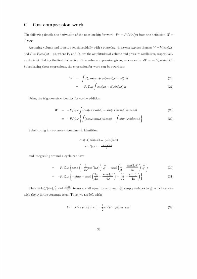
C Gas compression work

The following details the derivation of the relationship for work: W = PV sin (φ) from the denition W =

P dV :

Assuming volume and pressure act sinusoidally with a phase lag, φ, we can express them as V = V a cos(ωt)and P = P a cos(ωt + φ), where V a and P a are the amplitudes of volume and pressure oscillation, respectively

at the inlet. Taking the rst derivative of the volume expression given, we can write dV = − ωV a sin (ωt)dt .

Substituting these expressions, the expression for work can be rewritten:

W = P a cos(ωt + φ)(− ωV a sin (ωt))dt (26)

= − P a V a ω cos(ωt + φ)sin (ωt)dt (27)

Using the trigonometric identity for cosine addition,

W = − P a V a ω (cos(ωt)cos(φ) − sin (ωt)sin (φ))sinωtdt (28)

= − P a V a ω (cosωtsinωt )dtcosφ − sin 2(ωt)dtsinφ (29)

Substituting in two more trigonometric identities:

cos(ωt)sin (ωt) = 12 sin (2ωt)

sin 2(ωt) =1− cos 2ωt

2

and integrating around a cycle, we have

= − P a V a ω cosφ −1

2ωcos2(ωt) |

2 πω

0 − sinφt2

−sin (2ωt)

4ω|

2 πω

0 (30)

= − P a V a ω − sinφ − sinφ2π2ω

−sin (4ω)

4ω−

02

−sin (0)

4ω(31)

The sin(4 π)/ (4ω), 02 and sin (0)

4ω terms are all equal to zero, and 2π2ω simply reduces to π

ω , which cancels

with the ω in the constant term. Thus, we are left with:

W = PV πsin (φ)[rad ] =12

PV sin (φ)[degrees ] (32)

34



D MATLAB Code

%Pulse Tube Refrigerator Analysis

%Alisha Schor, [email protected]

%Define geometric parameters%All units SI (kg-m-s)

%Inches to meters multiplier

TOSI=0.0254;

%Swept Volume

dswept=1.364*TOSI;

lswept=0.1;

f=2; %Hz

Aswept=pi*dswept^2/4;

w=2*pi*f;

%Aftercooler (first HEX)

do=0.811*TOSI;

lo=0.7*TOSI;

Ao=pi*do^2/4;

Vo=Ao*lo;

%Regenerator

dr=1.364*TOSI;

lr=6*TOSI;

Ar=pi*dr^2/4;

Vr=Ar*lr;

%Cold HEX

dc=0.811*TOSI;lc=0.7*TOSI;

Ac=pi*dc^2/4;

Vc=Ac*lc;

%Pulse Tube

35



dpt=0.81*TOSI;

lpt=6*TOSI;

Apt=pi*dpt^2/4;

Vpt=Apt*lpt;

%Warm HEX

dh=0.811*TOSI;

lh=0.7*TOSI;

Ah=pi*dh^2/4;

Vh=Ah*lh;

%Choose temperatures

Tc=285; %K

Th=300; %K

Tr=(Th-Tc)/log(Th/Tc);

%NOTE: Either properties of air or properties

%of nitrogen must be commented prior to running

%this file.

%Properties of air

% R=287; %J/kg-K

% rhoo=1.229; %kg/m^3

% gamma=1.4;

% Patm=1.01e5; %Pa

% mu=1.5e-5; %Pa-s

% cp=1003; %J/kg-K

% kair=0.02544; %W/m-K

% nu=1.475e-5; %m^2/s

%Properties of nitrogen

R=290; %J/kg-K

36



rhoo=1.116; %kg/m^3

gamma=1.4;

Patm=1.01e5; %Pa

mu=1.8042e-5; %Pa-s

cp=1041.4; %J/kg-K

kair=0.02607; %W/m-K

nu=1.6231-5; %m^2/s

%Properties of copper

ccu=385; %J/kg-K

kcu=385; %W/m-K

rhocu=8960; %kg/m^3

%Chosen properties

Po=Patm;

Va=Aswept*lswept;

k=2:0.25:15;

k=10.^(-k);

37



%Pulse Tube Refrigerator Analysis

%Alisha Schor, [email protected]

%Run optrparam.m first to define parameters

%Time vector

t=0:0.005:2;

for j=1:length(k)

a(j)=R*Th/Po*(Vh/(R*Th)+(k(j)*rhoo/(i*w)));

b(j)=a(j)+Vpt/(gamma*Po)+Vh/(rhoo*R*Th)-1/rhoo*(Vh/(R*Th)+...

(k(j)*rhoo/(i*w))+k(j)/(i*w));

c(j)=R*Th/Po*(Vo/(R*Th)+Vr/(R*Tr)+Vc/(R*Tc)+b(j)*Po/(R*Tc)-...

b(j)*rhoo+a(j)*rhoo+rhoo*Vpt/(gamma*Po)+Vh/(R*Th)-a(j)*...

Po/(R*Th)+k(j)*rhoo/(i*w));

end

phase=angle(c)*180/pi;

MagC=abs(c);

% Calculate work and cooling power by choosing either

% pressure or volume amplitude.

% Pa=Va./MagC or Va=Pa.*MagC

Pa=Va./MagC;

Work=.5.*Pa.*Va.*sin(angle(c))*f;

DV3=Pa.*abs(b);

Qc=abs(-.5.*Pa.*DV3.*sin(angle(b))*f+i*w/(R*Tc)*(Pa*Vc+DV3*Po));

MaxWork=max(-Work)

MaxCooling=max(Qc)

for g=1:length(Work)

if Qc(g)==MaxCooling

38



OptimumK=k(g)

OptimumPhase=angle(c(g))*180/pi

MassFlow=OptimumK*rhoo*Pa(g);

VolFlow=OptimumK*Pa(g)

break

end

end

%Plot outputs

figure(1)

subplot(2,1,1)

semilogx(k,phase);xlabel(’k’);ylabel(’Phase (deg)’);

grid on

hold on

subplot(2,1,2)

semilogx(k,-Work,’k-.’);

hold on

semilogx(k,Qc,’b’);

xlabel(’k’);

ylabel(’Cooling Power (W)’);

grid on

%Valve sizing and Cv

%Based on Swagelok & Parker references

Q=OptimumK*Pa(g)*2118.88; %CFM

P1=(Po+Pa(g)/2)*0.0001450377; %PSIA

P2=Po*0.0001450377; %PSIA

%SG=1; %air

SG=0.967; %nitrogen T=(Th-273.15)*9/5+32+460; %"Absolute Temperature"

Cv=Q/16.05*sqrt(SG*T/(P1^2-P2^2))

39



%Required nozzle size based on mass flow rate

Pup=60; %upstream pressure in psi

Pup=Pup*6894.757; %upstream pressure in Pa

Anoz=MassFlow/(gamma^.5)*(2/(gamma+1)) (-(gamma+1)/(2*gamma-1))*sqrt(R*Th)/(Pup);

Dnoz=sqrt(4/pi*Anoz)

40



References

[1] R. Radebaugh, “Development of the pulse tube refrigerator as an efficient and reliable cryocooler,”

1999-2000.

[2] P. Neveu and C. Babo, “A simplied model for pulse tube refrigeration,” Cryogenics , vol. 40, no. 3,

pp. 191–201, 2000/3.

[3] P. Kittel, A. Kashani, J. M. Lee, and P. R. Roach, “General pulse tube theory,” Cryogenics , vol. 36,

no. 10, pp. 849–857, 1996/10.

[4] I. Urieli and D. M. Berchowitz, Stirling Cycle Engine Anaylsis . Bristol: Adam Hilger Ltd., 1984.

[5] G. Swift, Thermoacoustics: A unifying perspective for some engines and refrigerators . Los Alamos

National Laboratory: Unbublished, 2001.

[6] S. Rotundo, G. Hughel, A. Rebarchak, Y. Lin, and B. Farouk, “Design, construction and operation of

a traveling-wave pulse tube refrigerator,” in 14th International Cryocooler Conference , June 2006.

[7] F. P. Incorpera and D. P. DeWitt, Heat Transfer From Extended Surfaces , ch. 3.6, p. 126. Fundamentals

of Heat and Mass Transfer, Hoboken, NJ: John Wiley and Sons, 5th ed., 2002.

[8] S. Choi, K. Nam, and S. Jeong, “Investigation on the pressure drop characteristics of cryocooler regener-

ators under oscillating ow and pulsating pressure conditions,” Cryogenics , vol. 44, no. 3, pp. 203–210,

2004/3.

[9] P. C. T. de Boer, “Pressure heat pumping in the optr,” Advances in Cryogenic Engineering , vol. 41,

p. 1373, 1988.

[10] P. Kittel, “Ideal orice pulse tube refrigerator performance,” Cryogenics , vol. 32, no. 9, pp. 843–844,

1992.

[11] A. J. Organ, The Regenerator and the Stirling Engine . London, UK: JW Arrowsmith Ltd., 1997.

[12] A. J. Organ, pp. 79–85. Thermodynamics and Gas Dynamics of the Stirling Cycle Machine, New York:

Cambridge University Press, 1992.

[13] P. J. Storch and R. Radebaugh Advances in Cryogenic Engineering , vol. 33, p. 851, 1988.

Documents

Alisha Thesis