Embed Size (px)
Citation preview
Abstract
ANALYTICAL DERIVATION OF PSS PARAMETERSFOR GENERATOR WITH STATIC EXCITATION SYSTEM1
Zbigniew Lubośny / Gdansk University of TechnologyJanusz W. Białek / Durham University
I. NOMENCLATURE
Hjj – inertia constant, Eqj – q-axis steady-state internal emf,Iqj – stator current in the q-axis,K1-K6, T3j – parameters of linear model,KPSS, Ta-Tfj – PSS gain and time constants,Pg, Pref, Qgj – generator real, reference and reactive power,Rt, Xtj – step-up transformer resistance and reactance,Rs, Xsj – system resistance and reactance,Rl, Xlj – armature resistance and leakage reactance,Tg, Tmj – electromagnetic and mechanical torque,Ug, Uref, Usj – terminal, reference and infinite bus voltage,Xad, Xaqj – mutual reactance in d and q-axis,Xaduj – unsaturated mutual reactance in d-axis,X’dj – transient reactance in d-axis,Xfj – field circuit reactance,δ j – power angle,ω, ω0 – rotor speed, synchronous speed.
II. INTRODUCTIONProblem of damping electromechanical oscillations in electric power systems is not new. Since the 1950s,
when power systems started to get bigger and ever more stressed, engineers have been looking for synchro-nous generator controllers that could improve damping of oscillations.
The most popular tool for power system stability enhancement is the power system stabilizer (PSS) which provides an auxiliary control loop to the main automatic voltage regulator (AVR). PSS structure usually follows one of IEEE standards [1]. PSSs are usually of the single-input type with constant parameters (time-invariant) but two-input stabilizers are used too. PSS design is usually based on the compensation of plant frequency characteristics, optimization of defined quality indices, or shifting poles of the considered system to appropri-ate locations.
1 This work was supported by the Engineering and Physical Sciences Research Council, grant GR/S28082/01 “SUPERGEN: Future Network Tech-nologies”. .
Analytical derivation of pss parametersFor generator with static excitation system 79
This paper presents a methodology for PSS design which results in a PSS producing a nearly pure damping torque component in a wide frequency range. The derivation is based on the Heffron-Phillips single-machine infinite-bus-bar model and for a generator with static exciter and speed-based PSS. The choice of time constants is very simple and the only parameter still to be optimized is the PSS gain. Effectiveness of the PSS has been confirmed by tests con-ducted on single- and multi-machine power system model.
Other approaches of PSS design have been tried too like e.g. robust control techniques (LQG/LTR, H2, H∞, µ-synthesis), artificial intelligence based techniques (neural networks, fuzzy logic), or adaptive schemes but their practical implementation to the real power systems is so far marginal.
Design basis for PSS presently utilized in the power systems were provided in [2]. Practical methodology of PSS design has been proposed in [3] and further developed in [4]. Procedure of PSS design applicable to multi-machine power system was proposed in [5] and further developed in [6].
The practical methods of time-invariant PSS design are using damping torque concept and are based on GEP and P-Vr transfer functions. The GEP(s) is a transfer function between voltage reference of AVR and elec-trical torque. In case of the real object the transfer function between voltage reference and terminal voltage is measured. The P-Vr is a transfer function between voltage reference and electrical power, i.e., torque when the shaft dynamics of all machines are disabled. The both methodologies were lately compared and discussed in [7].
An interested reader can also consult [8] and [9] for a general description of the need for PSS and its design principles while reports [10] and [11] evaluate different approaches tried. Valuable practical considera-tions related to PSS design are presented in [12] and [13].
Damping torque concept is related to ideal PSS which, by definition [3], [11], provides damping torque only, i.e. transfer function between rotor speed and electrical torque is a real number over a range of frequen-cies of the rotor modes.
In general, the PSS should provide appropriate damping of electromechanical oscillations, despite it provides a damping torque only or also provides a synchronizing torque. In some circumstances (network configuration, network and machines operating point) it would be valuable to make the PSS to provide some synchronizing torque, especially for the low frequency modes, i.e. in case when synchronizing torque produced by machine and AVR becomes low. But so far there is no general answer to the question if, when, and in what amount PSS should provide synchronous torque.
Tests carried on multi-machine systems [5] show that non-ideal PSS can increase or decrease damping of given modes in contrary to ideal PSS. Despite this, the existing methods focuses on designing PSS which is as close to ideal as possible or is introducing slight under-compensation [12]. Therefore, goal of the paper is to derive equations allowing to calculate parameters of ideal PSS. Because the derivation is based on simplified model of synchronous machine while applying such PSS to non-simplified (or real) plant one can expect some degradation of its ideality, i.e. we achieve PSS introducing slight under-compensation.
Despite the time-invariant PSS concept and the GEP and P-Vr based methods since years has been deeply and with success exploited, an analytically derived equations for PSS parameters computing has not been pre-sented so far.
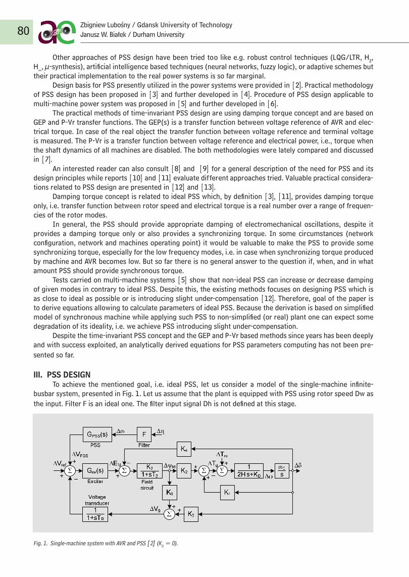
III. PSS DESIGNTo achieve the mentioned goal, i.e. ideal PSS, let us consider a model of the single-machine infinite-
busbar system, presented in Fig. 1. Let us assume that the plant is equipped with PSS using rotor speed Dw as the input. Filter F is an ideal one. The filter input signal Dh is not defined at this stage.
Fig. 1. Single-machine system with AVR and PSS [2] (KD = 0).
80Zbigniew Lubośny / Gdansk University of TechnologyJanusz W. Białek / Durham University
2
PSS to non-simplified (or real) plant one can expect some degradation of its ideality, i.e. we achieve PSS introducing slight under-compensation.
Despite the time-invariant PSS concept and the GEP and P-Vr based methods since years has been deeply and with success exploited, an analytically derived equations for PSS parameters computing has not been presented so far.
III. PSS DESIGN
To achieve the mentioned goal, i.e. ideal PSS, let us consider a model of the single-machine infinite-busbar system, presented in Fig. 1. Let us assume that the plant is equipped with PSS using rotor speed ∆ω as the input. Filter F is an ideal one. The filter input signal ∆η is not defined at this stage.
Fig. 1. Single-machine system with AVR and PSS [2] (KD = 0).
The electromagnetic torque ∆Tg can be defined as a function of the rotor angle ∆δ, the reference voltage ∆Vref and the rotor speed ∆ω :
ωδδ ∆⋅+∆⋅+∆⋅=∆ )()()( sTVsTsTT PSSrefVg (1)
where Tδ(s), TV(s), TPSS(s) are some transfer functions that depend on the plant’s parameters K1-K6, T3 and on the controller’s transfer functions, defined by Gex(s) and GPSS(s). What is important here, the PSS transfer function GPSS(s)appears in the TPSS(s) transfer function only.
The electromagnetic torque produced by the PSS is equal to:
ωω ∆+++
+=∆⋅=∆)()1)(1(
)1)(()()(633
32sGKKsTsT
sTsGsGKKsTTexR
RPSSexPSSPSS (2)
After introducing the PSS and the AVR transfer functions to (2) the TPSS(s) function can be written in form:
Ksb
saKsT M
j
jj
N
i
ii
PSSPSS =∑+
∑+=
=
=
1
1
1
1)( (3)
The electromagnetic torque ∆TPSS produced by the PSS will be in phase with the rotor speed ∆ω, i.e. we will achieve the ideal power system stabilizer, when the transfer function TPSS(s) will become real.
The function (3) takes form of a gain K when, for example, the following requirement is fulfilled:
iiMNNiba =∀
== ,...1 (4)
i.e. the numerator and the denominator coefficients, located at the same positions, are equal to each other. When this requirement is fulfilled the PSS is providing the damping torque only for the all frequencies of oscillations.
The search for such PSS means deriving formulas defining the PSS parameters that fulfill requirement (4). To find an analytical solution to the problem it is necessary to make some initial assumptions, i.e.: • allow the PSS’s numerator rank to be higher than the
denominator rank, • allow the AVR parameters to be defined by the derived
equations, • neglect dynamics of some components with small time
constant, e.g. voltage transducer.
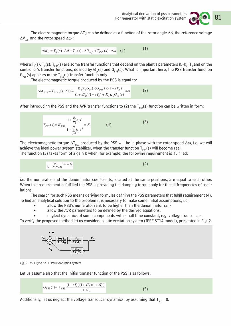
To verify the proposed method let us consider a static excitation system (IEEE ST1A model), presented in Fig. 2.
Fig. 2. IEEE type ST1A static excitation system
Let us assume also that the initial transfer function of the PSS is as follows:
d
cbaPSSPSS sT
sTsTsTKsG+
+++=1
)1)(1)(1()( (5)
Additionally, let us neglect the voltage transducer dynamics, by assuming that TR = 0.
For a such defined plant the parameters of the PSS that provides damping torque only are defined by (6):
Aa TT = , Bb TT = , A
Fc KKK
TT631 +
= , Fd TT = (6)
Simultaneously, some of the AVR parameters have to be defined as follow:
3TTC = , 3
63 TTTKKK BA
F = , 3TTTTTT BA
BAF −+= (7)
The Eqs. (6) and (7) define the ideal PSS of a given structure.
Gain K which is a measure of the damping torque provided by the PSS, is here equal to:
A
PSSAKKK
KKKKK63
321 +
= (8)
In the real power systems the AVR, presented in Fig. 2, is also (even often) utilized in one of the following form: • with existing feedback loop (KF ≠ 0) but without transient
gain reduction block (TGR) (TB = TC), • with existing transient gain reduction block (TB ≠ TC) but
without feedback loop (KF = 0). In the first case, i.e. for synchronous generator equipped
with AVR without TGR the PSS and AVR parameters are
The electromagnetic torque ∆Tg can be defined as a function of the rotor angle ∆δ, the reference voltage ∆Vref and the rotor speed ∆ω : (1)
where Tδ(s), TV(s), TPSS(s) are some transfer functions that depend on the plant’s parameters K1-K6, T3 and on the controller’s transfer functions, defined by Gex(s) and GPSS(s). What is important here, the PSS transfer function GPSS(s) appears in the TPSS(s) transfer function only.
The electromagnetic torque produced by the PSS is equal to:
(2)
After introducing the PSS and the AVR transfer functions to (2) the TPSS(s) function can be written in form:
(3)
The electromagnetic torque ∆TPSS produced by the PSS will be in phase with the rotor speed ∆ω, i.e. we will achieve the ideal power system stabilizer, when the transfer function TPSS(s) will become real. The function (3) takes form of a gain K when, for example, the following requirement is fulfilled:
(4)
i.e. the numerator and the denominator coefficients, located at the same positions, are equal to each other. When this requirement is fulfilled the PSS is providing the damping torque only for the all frequencies of oscil-lations.
The search for such PSS means deriving formulas defining the PSS parameters that fulfill requirement (4). To find an analytical solution to the problem it is necessary to make some initial assumptions, i.e.: • allow the PSS’s numerator rank to be higher than the denominator rank, • allow the AVR parameters to be defined by the derived equations, • neglect dynamics of some components with small time constant, e.g. voltage transducer.To verify the proposed method let us consider a static excitation system (IEEE ST1A model), presented in Fig. 2.
Fig. 2. IEEE type ST1A static excitation system
Let us assume also that the initial transfer function of the PSS is as follows:
(5)
Additionally, let us neglect the voltage transducer dynamics, by assuming that TR = 0.
81Analytical derivation of pss parameters
For generator with static excitation system
4
Rys. 1. Liniowy model układu jednomaszynowego z regulatorem napięcia (RN) i stabilizatorem syste-
mowym (PSS), (KD = 0)
Moment elektromagnetyczny ∆Me moŜna zdefiniować jako funkcję kąta mocy ∆δ, napięcia zadanego
generatora ∆Vref oraz prędkości kątowej wirnika generatora ∆ω :
ωδδ ∆⋅+∆⋅+∆⋅=∆ )()()( sTUsTsTM PSSrefUe (1)
gdzie Tδ(s), TU(s), TPSS(s) są pewnymi transmitancjami zaleŜnymi od parametrów obiektu K1-K6, T3 oraz od
transmitancji regulatora napięcia generatora synchronicznego Gex(s) oraz transmitancji stabilizatora
systemowego GPSS(s). Co istotne, transmitancja stabilizatora systemowego GPSS(s) występuje tylko w
funkcji TPSS(s).
Moment elektromagnetyczny wytwarzany przez stabilizator systemowy jest równy:
ωω ∆+++
+=∆⋅=∆
)()1)(1(
)1)(()()(
633
32
sGKKsTsT
sTsGsGKKsTM
exR
RPSSexPSSPSS (2)
Po uwzględnieniu w zaleŜności (2) transmitancji stabilizatora systemowego i regulatora napięcia
generatora synchronicznego, transmitancję TPSS(s) (zaleŜność 2) moŜna przedstawić w postaci:
Ks
saKsT M
j
jj
N
i
ii
PSSPSSb
=+
+=
∑
∑
=
=
1
1
1
1)( (3)
Moment (fazor momentu) elektromagnetyczny ∆TPSS, wytwarzany przez stabilizator systemowy PSS,
będzie w fazie z prędkością (fazorem prędkości) wirnika generatora ∆ω, tzn. uzyskamy idealny stabilizator
systemowy, gdy transmitancja TPSS(s) będzie liczbą lub funkcją rzeczywistą.
ZaleŜność (3) staje się równa liczbie rzeczywistej K, gdy np. spełniona jest następująca zaleŜność:
5
iiMNNiba =∀
== ,...1 (4)
tzn. gdy współczynniki wielomianu licznika i mianownika transmitancji (3), znajdujące się na tych samych
pozycjach w wielomianach, będą sobie równe. Spełnienie warunku (4) powoduje, Ŝe rozwaŜany
stabilizator systemowy będzie wytwarzał tylko moment tłumiący o stałej, tj. niezaleŜnej od częstotliwości
wartości, dla dowolnej częstotliwości kołysań elektromechanicznych.
Synteza rozwaŜanego tu stabilizatora systemowego sprowadza się zatem do określenia parametrów
stabilizatora, które spełniają warunek (4).
W celu analitycznego rozwiązania problemu naleŜy przyjąć dodatkowe załoŜenia, a w tym:
• dopuścić rząd wielomianu licznika wyŜszy niŜ wielomianu mianownika transmitancji
• dopuścić moŜliwość definiowania parametrów regulatora napięcia generatora przez wyprowadzone
zaleŜności, tj. w celu spełnienia warunku (4)
• pominąć elementy modelu obiektu o małych stałych czasowych, np. przetwornika pomiarowego
napięcia generatora.
W celu weryfikacji zaproponowanej metody syntezy stabilizatora systemowego przyjmijmy, Ŝe generator
synchroniczny wyposaŜony jest w statyczny układ wzbudzenia i regulacji napięcia typu IEEE ST1A, tj. jak
przedstawiony na rys. 2.
Rys. 2. Model statycznego układu wzbudzenia i regulacji napięcia typu IEEE ST1A
ZałóŜmy wstępnie transmitancję stabilizatora systemowego o postaci jak (5):
d
cbaPSSPSS sT
sTsTsTKsG+
+++=1
)1)(1)(1()( (5)
Ponadto pomińmy dynamikę przetwornika pomiarowego napięcia generatora, przyjmując TR = 0.
Dla tak zdefiniowanego obiektu parametry stabilizatora systemowego wytwarzającego tylko moment
tłumiący określone są następującymi zaleŜnościami:
Aa TT = , Bb TT = , A
Fc KKK
TT631 +
= , Fd TT = (6)
Równocześnie pewne parametry regulatora napięcia generatora muszą być równe:
For a such defined plant the parameters of the PSS that provides damping torque only are defined by (6):
(6)
Simultaneously, some of the AVR parameters have to be defined as follow:
(7)
The Eqs. (6) and (7) define the ideal PSS of a given structure.Gain K which is a measure of the damping torque provided by the PSS, is here equal to:
(8)
In the real power systems the AVR, presented in Fig. 2, is also (even often) utilized in one of the following form: • with existing feedback loop (KF ≠ 0) but without transient gain reduction block (TGR) (TB = TC), • with existing transient gain reduction block (TB ≠ TC) but without feedback loop (KF = 0).In the first case, i.e. for synchronous generator equipped with AVR without TGR the PSS and AVR parameters are defined by the following equations
(9)
In the second case, i.e. for synchronous generator equipped with AVR with TGR but without feedback loop, the PSS and AVR parameters are defined as follows:
(10)
In the second case, in contrary to the previous cases, i.e. for controllers defined by (6) and (7) or by (9), the time constants defined by (10) satisfy conditions a1 = b1, a3 = b3 (Eq. (4)) but not satisfy at the same time condition a2 = b2. This means that the PSS produces some synchronizing torque also. Fortunately, because of the imagi-nary part of TPSS is proportional to a2 – b2 ≈ T3TA while TA is small the imaginary part of TPSS and simultaneously the synchronizing torque are small too. To make the PSS realizable the numerator and the denominator rank of its transfer function should be equal. Then the denominator should be supplemented by two inertia elements, what leads the PSS to the following form:
(11)
The values of time constants Te and Tf should be chosen small, e.g. Te = Tf < 0.01 s, in order not to introduce an significant phase shift to GPSS(s) for frequencies in the electromechanical oscillations range, i.e. 0.1–2.5 Hz. Introduction of the both small time constants practically does not affect the PSS effectiveness.
82Zbigniew Lubośny / Gdansk University of TechnologyJanusz W. Białek / Durham University
6
3TTC = , 3
63 TTTKKK BA
F = , 3TTTTTT BA
BAF −+= (7)
Wówczas zaleŜności (6) i (7) definiują tzw. idealny stabilizator systemowy.
Współczynnik K, będący miarą momentu tłumiącego wytwarzanego przez stabilizator systemowy, jest
wówczas równy:
A
PSSA
KKKKKKKK63
321+
= (8)
W rzeczywistości regulator napięcia generatora synchronicznego z rys. 2 dość często występuje w jednej z
następujących postaci (struktur):
• z pętlą sprzęŜenia zwrotnego (KF ≠ 0) ale bez bloku TGR (Transient Reduction Gain) (TB = TC)
• z blokiem TGR (TB ≠ TC), ale bez pętli sprzęŜenia zwrotnego (KF = 0).
W pierwszym przypadku, tj. dla generatora synchronicznego z regulatorem napięcia generatora bez bloku
TGR w swojej strukturze, parametry stabilizatora systemowego i regulatora napięcia definiują następujące
zaleŜności:
Aa TT = , A
b KKKTT
63
31 +
= , dc TT = (9)
AF TKKK 63= , 3TTF =
W drugim przypadku, tj. dla generatora synchronicznego z regulatorem napięcia generatora z blokiem TGR
w swojej strukturze parametry stabilizatora systemowego i regulatora napięcia definiują zaleŜności:
Aa TT = , 3TTb = , A
Bc KKK
TT631 +
= , ACd TTTT +== 3 (10)
W przypadku drugim, w porównaniu z pierwszym, tj. dla regulatorów definiowanych przez zaleŜności (6) i
(7) oraz przez (9), stałe czasowe definiowane zaleŜnością (10) prowadzą do spełniania warunków a1 = b1,
a3 = b3 [zaleŜność (4)], ale nie umoŜliwiają spełnienia warunku a2 = b2. Oznacza to, Ŝe tak określony
stabilizator systemowy wytwarza równieŜ, oprócz momentu tłumiącego, pewien moment synchronizujący.
PoniewaŜ jednak część urojona transmitancji TPSS jest proporcjonalna do a2 - b2 ≈ T3TA, gdzie wartość TA
jest mała, urojona część transmitancji TPSS i równocześnie moment synchronizujący są równieŜ małe.
W celu uzyskania realizowalności stabilizatora systemowego rząd wielomianu licznika jego transmitancji
nie moŜe być większy od rzędu wielomianu mianownika. Aby to uzyskać, tj. doprowadzić do stanu, w
którym rząd wielomianu licznika i mianownika transmitancji stabilizatora systemowego będą równe,
naleŜy uzupełnić mianownik transmitancji z zaleŜności (5) do postaci jak poniŜej:
7
)1)(1)(1()1)(1)(1()(
fed
cbaPSSPSS sTsTsT
sTsTsTKsG++++++= (11)
Wartości stałych czasowych Te i Tf powinny być na tyle małe, np. Te = Tf < 0,01 s, aby w transmitancji
GPSS(s) nie powodować znaczącego przesunięcia fazy z zakresu częstotliwości odpowiadających
częstotliwościom kołysań elektromechanicznych w systemie elektroenergetycznym, tj. 0,1–2,5 Hz.
PowyŜsza modyfikacja transmitancji stabilizatora systemowego praktycznie nie zmniejsza efektywności
rozwaŜanego stabilizatora systemowego.
Wyprowadzone zaleŜności pozwalają na sformułowanie następujących uwag:
• Parametry stabilizatora systemowego i regulatora napięcia generatora definiowane przez powyŜsze
zaleŜności, pozwalające stabilizatorowi systemowemu wytwarzać tylko moment tłumiący, zaleŜą od
punktu pracy generatora synchronicznego, parametrów maszyny i impedancji zewnętrznej (widzianej z
szyn generatora synchronicznego).
• PowyŜsze zaleŜności związane są z eliminowaniem się zer i biegunów transmitancji. Przykładowo,
pewne stałe czasowe w liczniku transmitancji stabilizatora systemowego są równe stałym czasowym
mianownika regulatora napięcia lub obwodu wzbudzenia maszyny (i odwrotnie). Sposób określania
niektórych stałych czasowych wydaje się intuicyjny, podczas gdy sposób definiowania innych stałych
czasowych i współczynnika wzmocnienia w pętli sprzęŜenia zwrotnego nie jest juŜ tak oczywisty.
• ZaleŜności (7), (9) i (10) określają wartości niektórych parametrów regulatora napięcia, które pozwalają
stabilizatorowi systemowemu PSS na optymalność. PowyŜsze, tj. konieczność modyfikacji wartości
nastaw regulatora napięcia, moŜe być traktowane jako ograniczenie proponowanej metody. NaleŜy
jednak podkreślić, Ŝe wartości parametrów regulatora napięcia, obliczone za pomocą powyŜszych
zaleŜności, często są bliskie nastawianym w regulatorach rzeczywistych. Parametry regulatora napięcia
generatora, określone przez zaleŜności (7), (9) oraz (10), pozwalają na poprawną pracę generatora
synchronicznego równieŜ po wyłączeniu stabilizatora systemowego oraz jego wydzieleniu się z pracy w
systemie elektroenergetycznym.
W przypadku regulatora napięcia bez pętli sprzęŜenia zwrotnego własności dynamiczne obiektu mogą
być niezaleŜnie kształtowane przez parametry KA i TB, które nie są definiowane przez zaproponowane
zaleŜności. W przypadku regulatora napięcia z pętlą sprzęŜenia zwrotnego, ale bez bloku TGR,
własności dynamiczne obiektu mogą być niezaleŜnie kształtowane tylko za pomocą współczynnika
wzmocnienia KA, a własności dynamiczne obiektu pracującego poza systemem elektroenergetycznym
(w tym na potrzeby własne) względnie silnie zaleŜą od stałej czasowej TA. Im mniejsza jest jej wartość,
tym lepsze własności dynamiczne obiektu.
• Wartości stałych czasowych stabilizatora systemowego zaleŜą od wartości parametrów regulatora
5
iiMNNiba =∀
== ,...1 (4)
tzn. gdy współczynniki wielomianu licznika i mianownika transmitancji (3), znajdujące się na tych samych
pozycjach w wielomianach, będą sobie równe. Spełnienie warunku (4) powoduje, Ŝe rozwaŜany
stabilizator systemowy będzie wytwarzał tylko moment tłumiący o stałej, tj. niezaleŜnej od częstotliwości
wartości, dla dowolnej częstotliwości kołysań elektromechanicznych.
Synteza rozwaŜanego tu stabilizatora systemowego sprowadza się zatem do określenia parametrów
stabilizatora, które spełniają warunek (4).
W celu analitycznego rozwiązania problemu naleŜy przyjąć dodatkowe załoŜenia, a w tym:
• dopuścić rząd wielomianu licznika wyŜszy niŜ wielomianu mianownika transmitancji
• dopuścić moŜliwość definiowania parametrów regulatora napięcia generatora przez wyprowadzone
zaleŜności, tj. w celu spełnienia warunku (4)
• pominąć elementy modelu obiektu o małych stałych czasowych, np. przetwornika pomiarowego
napięcia generatora.
W celu weryfikacji zaproponowanej metody syntezy stabilizatora systemowego przyjmijmy, Ŝe generator
synchroniczny wyposaŜony jest w statyczny układ wzbudzenia i regulacji napięcia typu IEEE ST1A, tj. jak
przedstawiony na rys. 2.
Rys. 2. Model statycznego układu wzbudzenia i regulacji napięcia typu IEEE ST1A
ZałóŜmy wstępnie transmitancję stabilizatora systemowego o postaci jak (5):
d
cbaPSSPSS sT
sTsTsTKsG+
+++=1
)1)(1)(1()( (5)
Ponadto pomińmy dynamikę przetwornika pomiarowego napięcia generatora, przyjmując TR = 0.
Dla tak zdefiniowanego obiektu parametry stabilizatora systemowego wytwarzającego tylko moment
tłumiący określone są następującymi zaleŜnościami:
Aa TT = , Bb TT = , A
Fc KKK
TT631 +
= , Fd TT = (6)
Równocześnie pewne parametry regulatora napięcia generatora muszą być równe:
6
3TTC = , 3
63 TTTKKK BA
F = , 3TTTTTT BA
BAF −+= (7)
Wówczas zaleŜności (6) i (7) definiują tzw. idealny stabilizator systemowy.
Współczynnik K, będący miarą momentu tłumiącego wytwarzanego przez stabilizator systemowy, jest
wówczas równy:
A
PSSA
KKKKKKKK63
321+
= (8)
W rzeczywistości regulator napięcia generatora synchronicznego z rys. 2 dość często występuje w jednej z
następujących postaci (struktur):
• z pętlą sprzęŜenia zwrotnego (KF ≠ 0) ale bez bloku TGR (Transient Reduction Gain) (TB = TC)
• z blokiem TGR (TB ≠ TC), ale bez pętli sprzęŜenia zwrotnego (KF = 0).
W pierwszym przypadku, tj. dla generatora synchronicznego z regulatorem napięcia generatora bez bloku
TGR w swojej strukturze, parametry stabilizatora systemowego i regulatora napięcia definiują następujące
zaleŜności:
Aa TT = , A
b KKKTT
63
31 +
= , dc TT = (9)
AF TKKK 63= , 3TTF =
W drugim przypadku, tj. dla generatora synchronicznego z regulatorem napięcia generatora z blokiem TGR
w swojej strukturze parametry stabilizatora systemowego i regulatora napięcia definiują zaleŜności:
Aa TT = , 3TTb = , A
Bc KKK
TT631 +
= , ACd TTTT +== 3 (10)
W przypadku drugim, w porównaniu z pierwszym, tj. dla regulatorów definiowanych przez zaleŜności (6) i
(7) oraz przez (9), stałe czasowe definiowane zaleŜnością (10) prowadzą do spełniania warunków a1 = b1,
a3 = b3 [zaleŜność (4)], ale nie umoŜliwiają spełnienia warunku a2 = b2. Oznacza to, Ŝe tak określony
stabilizator systemowy wytwarza równieŜ, oprócz momentu tłumiącego, pewien moment synchronizujący.
PoniewaŜ jednak część urojona transmitancji TPSS jest proporcjonalna do a2 - b2 ≈ T3TA, gdzie wartość TA
jest mała, urojona część transmitancji TPSS i równocześnie moment synchronizujący są równieŜ małe.
W celu uzyskania realizowalności stabilizatora systemowego rząd wielomianu licznika jego transmitancji
nie moŜe być większy od rzędu wielomianu mianownika. Aby to uzyskać, tj. doprowadzić do stanu, w
którym rząd wielomianu licznika i mianownika transmitancji stabilizatora systemowego będą równe,
naleŜy uzupełnić mianownik transmitancji z zaleŜności (5) do postaci jak poniŜej:
The derived equations allow as to formulate the following remarks:• The PSS and AVR parameters, defined by above Eqs., allowing the PSS to produce damping torque only
depend on plant’s operating point, machine data, and external impedance. This confirms common know-ledge that parameters of optimal controller of synchronous generator should vary.
• The equations show some type of zero/poles cancellation, i.e. some time constants in numerator of the PSS transfer function are equal to time constants in denominator of AVR and machine field circuit transfer function (and opposite). Definition of these time constants seems to be intuitive while definition of other time constants and feedback loop gain seems not so obvious.
• Equations (7), (9) and (10) define some parameters of AVR that allow the PSS to perform optimally. That can be treated as some disadvantage of the method, but the parameters are often close to the one defi-ned for existing AVRs. The AVR parameters defined by (7), (9) and (10) allow to proper operation of plant also after PSS disconnection, e.g. at open-circuit.In case of AVR without feedback loop, dynamic properties of the plant can be independently shaped by
KA and TB, that are not defined by the derived rules. In case of AVR with feedback loop but without TGR the plant’s dynamic properties can be independently shaped by KA only. In this case the dynamic properties of plant operating at open-circuit relatively highly depend on TA. The smaller value of TA ensures the better dynamic properties of the plant.
• The derived time constants of PSS depend both from voltage controller parameters and from plant ope-rating point. The plant parameters variation as function of operating point and external impedance is discussed in [2]
and [3] and will not be repeated here. Variation of the PSS time constants that are proportional to T3 is relatively small. T3 is low sensitive to
plant load and higher sensitive to external impedance (especially to resistance). Variation of time constant Tc in (6) and (10) and Tb in (9) is high only for operating points located close and behind the stability limit of plant equipped with AVR only.
The PSS gain definition is a separate task not related to the time constants definition. The PSS gain defini-tion, especially for the multi-machine power system is not easy task, but can be done by utilisation of various method, e.g. mentioned above.
Below the simple way of the PSS gain definition is proposed. For plant from Fig. 1 the equation of motion, taking into account (1) and assuming that TPSS(s) transfer function has only a real part (i.e. the PSS is ideal), can be written in the form:
(12)
where Tδ S and Tδ D are the frequency-dependent real and imaginary parts of transfer function Tδ(s) defining synchronising and damping components of torque produced by the machine and AVR.Equation (12) defines a standard oscillatory element. For such element the PSS gain, assuming (8), can be cal-culated as the function of the required damping ratio ξ using:
(13)
The gain KPSS is a nonlinear function of the plant parameters, state and frequency of oscillations.
IV. PSS VERIFICATION IN A SINGLE-MACHINE SYSTEMFor the PSS verification in a single-machine system parameters of synchronous generator marked as G2 in
Appendix have been used. Data for that unit has been taken from real generating unit. The unit is equipped with AVR type ST1A without feedback loop. The external impedance, i.e. behind step-up transformer was assumed as equal to Zs = 0.007 + j0.08 p.u. (rated to machine base).
Fig. 3 shows magnitude and angle of TPSS(s) for various values of reactive power and frequency, when real power is equal to the rated one. The PSS and AVR parameters have been recalculated, using (10), at each operating point. The gain KPSS was assumed to be equal to one.
83Analytical derivation of pss parameters
For generator with static excitation system
8
napięcia generatora oraz od stanu pracy generatora.
Zmienność parametrów obiektu (współczynników K1-K6) w funkcji zmienności punktu pracy generatora
i wartości impedancji zewnętrznej jest dyskutowana w pracach [2] i [3] i nie będzie tu powtarzana.
Zmienność stałych czasowych stabilizatora systemowego w funkcji stałej czasowej obiektu T3 jest
względnie mała. Stała czasowa T3 jest mało wraŜliwa na punkt pracy generatora i bardziej wraŜliwa na
wartość impedancji (szczególnie rezystancji) zewnętrznej. Zmienność stałej czasowej Tc w zaleŜności
(6) i (10) oraz stałej czasowej Tb w zaleŜności (9) jest duŜa tylko dla punktów pracy generatora
synchronicznego, ulokowanych w pobliŜu granicy stabilności lokalnej obiektu pracującego tylko z
regulatorem napięcia.
Zadanie określenia współczynnika wzmocnienia stabilizatora systemowego jest zadaniem niezaleŜnym od
przedstawionej metody określania stałych czasowych stabilizatora. Zadanie to, szczególnie w systemie
wielomaszynowym, nie jest zadaniem łatwym. Jest ono realizowane w róŜnoraki sposób, a w tym w sposób
pokazany powyŜej.
PoniŜej przedstawiono prosty sposób określania współczynnika wzmocnienia stabilizatora systemowego.
Dla obiektu z rys. 1 równanie ruchu, biorąc pod uwagę (1) i zakładając, Ŝe transmitancja TPSS(s) jest
funkcją rzeczywistą, tj. stabilizator systemowy jest idealny, moŜna napisać w postaci:
)(22
)22
( 0002refVm
jj
S
j
D
j
PSS VTTHH
TsH
TH
Ts ∆−∆=∆+∆++∆ ωδωδω
ωδ δδ (12)
gdzie TδS i TδD są zaleŜnymi od częstotliwości składowymi transmitancji Tδ(s), definiującymi odpowiednio
momenty synchronizujący i tłumiący, wytwarzane przez maszynę i regulator napięcia generatora.
Równanie (12) jest równaniem elementu (obiektu) oscylacyjnego 2. rzędu. Dla takiego elementu (obiektu)
współczynnik wzmocnienia stabilizatora systemowego, przyjmując (8), moŜna obliczyć jako funkcję
wymaganego współczynnika wzmocnienia ξ z zaleŜności:
)22(1 00
32
63ωωωξ δδ DSj
A
APSS TTH
KKKKKKK −+= (13)
Współczynnik wzmocnienia KPSS jest tu nieliniową funkcją parametrów obiektu, stanu pracy obiektu oraz
częstotliwości oscylacji.
IV. WERYFIKACJA STABILIZATORA SYSTEMOWEGO W UKŁADZIE JEDNOMASZYNOWYM
Poprawność zaproponowanej metody zweryfikowano wstępnie w układzie jednomaszynowym,
wykorzystując generator G2 według danych zawartych w załączniku. Generator synchroniczny jest tu
wyposaŜony w statyczny układ wzbudzenia i regulacji napięcia typu ST1A, bez pętli sprzęŜenia zwrotnego.
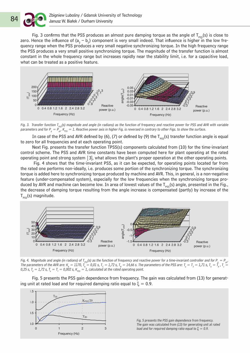
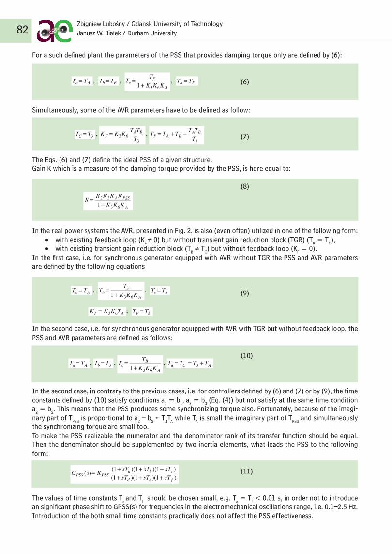
Fig. 3 confirms that the PSS produces an almost pure damping torque as the angle of TPSS(s) is close to zero. Hence the influence of (a2 – b2) component is very small indeed. That influence is higher in the low fre-quency range when the PSS produces a very small negative synchronizing torque. In the high frequency range the PSS produces a very small positive synchronizing torque. The magnitude of the transfer function is almost constant in the whole frequency range but increases rapidly near the stability limit, i.e. for a capacitive load, what can be treated as a positive feature.
Fig. 3. Transfer function TPSS(s) magnitude and angle (in radians) as the function of frequency and reactive power for PSS and AVR with variable parameters and for Pg = Pgn. KPSS = 1. Reactive power axis in higher Fig. is reversed in contrary to other Figs. to show the surface.
In case of the PSS and AVR defined by (6), (7) or defined by (9) the TPSS(s) transfer function angle is equal to zero for all frequencies and at each operating point.
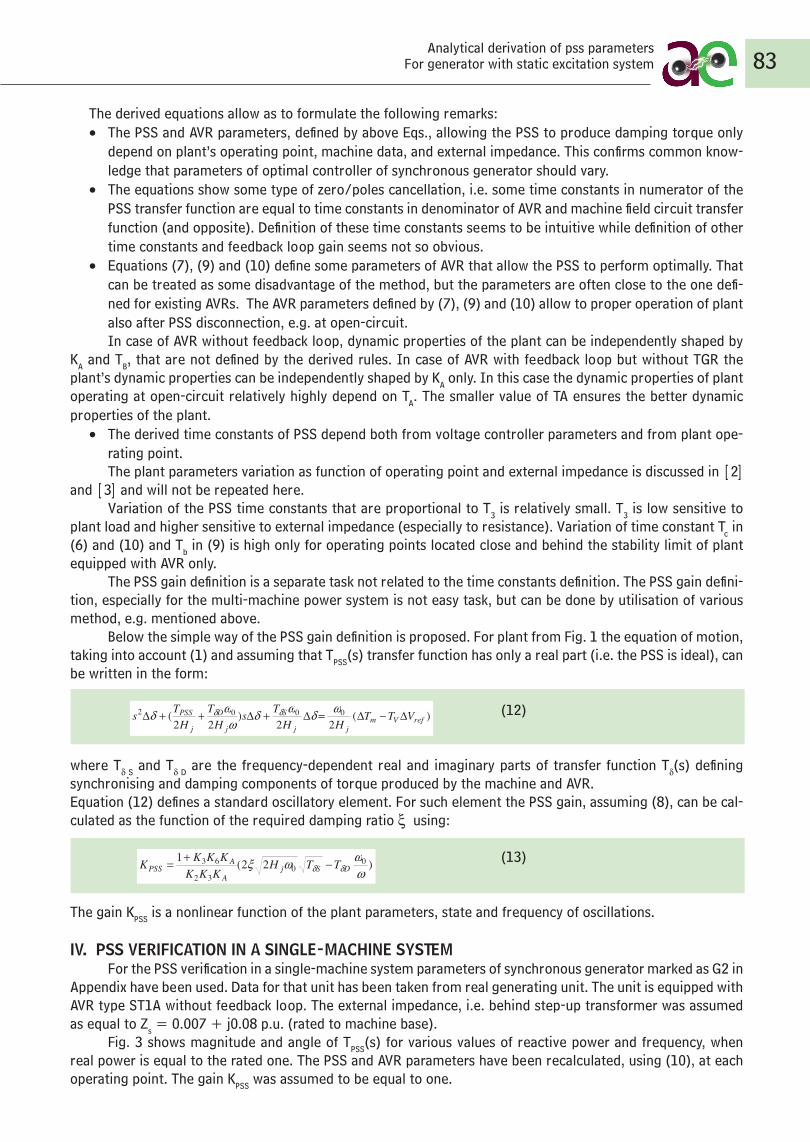
Next Fig. presents the transfer function TPSS(s) components calculated from (10) for the time-invariant control scheme. The PSS and AVR time constants have been computed here for plant operating at the rated operating point and strong system [3], what allows the plant’s proper operation at the other operating points.
Fig. 4 shows that the time-invariant PSS, as it can be expected, for operating points located far from the rated one performs non-ideally, i.e. produces some portion of the synchronizing torque. The synchronizing torque is added here to synchronizing torque produced by machine and AVR. This, in general, is a non-negative feature (under-compensated system), especially for the low frequencies when the synchronizing torque pro-duced by AVR and machine can become low. In area of lowest values of the TPSS(s) angle, presented in the Fig., the decrease of damping torque resulting from the angle increase is compensated (partly) by increase of the TPSS(s) magnitude.
Fig. 4. Magnitude and angle (in radians) of TPSS(s) as the function of frequency and reactive power for a time-invariant controller and for Pg = Pgn. The parameters of the AVR are: KA = 1170, TA = 0,01 s, TC = 1,72 s, TB = 14,66 s. The parameters of the PSS are: Ta = T3 = 1,71 s, Tb = TA , Tc = 0,25 s, Td = 1,72 s, Te = Tf = 0,002 s, KPSS = 1, calculated at the rated operating point.
Fig. 5 presents the PSS gain dependence from frequency. The gain was calculated from (13) for generat-ing unit at rated load and for required damping ratio equal to ξ = 0.9.
84Zbigniew Lubośny / Gdansk University of TechnologyJanusz W. Białek / Durham University
Fig. 5 presents the PSS gain dependence from frequency. The gain was calculated from (13) for generating unit at rated load and for required damping ratio equal to ξ = 0.9.
4
been recalculated, using (10), at each operating point. The gain KPSS was assumed to be equal to one.
Fig. 3 confirms that the PSS produces an almost pure damping torque as the angle of TPSS(s) is close to zero. Hence the influence of (a2 – b2) component is very small indeed. That influence is higher in the low frequency range when the PSS produces a very small negative synchronizing torque. In the high frequency range the PSS produces a very small positive synchronizing torque. The magnitude of the transfer function is almost constant in the whole frequency range but increases rapidly near the stability limit, i.e. for a capacitive load, what can be treated as a positive feature.
050
100150200
|Tps
s|
0 0.4 0.8 1.2 1.6 2 2.4 2.8 3.2
-0 .3-0 .10 .10 .30 .50 .70 .9
Frequency (Hz)
Reactive power (p.u.)
-0.05-0.03-0.010.010.030.05
angl
e(T p
ss)
0 0.4 0.8 1.2 1.6 2 2.4 2.8 3.2-0.3-0.10.10.30.50.70.9
Frequency (Hz)
Reactive power (p.u.)
Fig. 3. Transfer function TPSS(s) magnitude and angle (in radians) as the function of frequency and reactive power for PSS and AVR with variable parameters and for Pg = Pgn. KPSS = 1. Reactive power axis in higher Fig. is reversed in contrary to other Figs. to show the surface.
In case of the PSS and AVR defined by (6), (7) or defined by (9) the TPSS(s) transfer function angle is equal to zero for all frequencies and at each operating point.
Next Fig. presents the transfer function TPSS(s) components calculated from (10) for the time-invariant control scheme. The PSS and AVR time constants have been computed here for plant operating at the rated operating point and strong system [3], what allows the plant’s proper operation at the other operating points.
Fig. 4 shows that the time-invariant PSS, as it can be expected, for operating points located far from the rated one performs non-ideally, i.e. produces some portion of the synchronizing torque. The synchronizing torque is added here to synchronizing torque produced by machine and AVR. This, in general, is a non-negative feature (under-compensated system), especially for the low frequencies when the synchronizing torque produced by AVR and machine can
become low. In area of lowest values of the TPSS(s) angle, presented in the Fig., the decrease of damping torque resulting from the angle increase is compensated (partly) by increase of the TPSS(s) magnitude.
01020304050
|Tps
s|
0 0.4 0.8 1.2 1.6 2 2.4 2.8 3.2-0.3-0.10.10.3
0.50.70.9
Frequency (Hz)
Reactive power (p.u.)
-1.5
-1
-0.5
0
angl
e(T p
ss)
0 0.4 0.8 1.2 1.6 2 2.4 2.8 3.2-0.3-0.10.1
0.30.50.70.9
Frequency (Hz)
Reactive power (p.u.)
Fig. 4. Magnitude and angle (in radians) of TPSS(s) as the function of frequency and reactive power for a time-invariant controller and for Pg = Pgn. The parameters of the AVR are: KA = 1170, TA = 0.01 s, TC = 1.72 s, TB = 14.66 s. The parameters of the PSS are: Ta = T3 = 1.71 s, Tb = TA , Tc = 0.25 s, Td = 1.72 s, Te = Tf = 0.002 s, KPSS = 1, calculated at the rated operating point.
Fig. 5 presents the PSS gain dependence from frequency. The gain was calculated from (13) for generating unit at rated load and for required damping ratio equal to ξ = 0.9.
0.0
0.5
1.0
1.5
0 1 2 3Frequency (Hz)
Fig. 5. PSS gain and the synchronizing and damping components of transfer function Tδ(s), calculated at rated operating point.
The Fig. shows that for given plant (G2) keeping the PSS gain equal to 20 allow us to keep the damping ratio not lower than 0.9 for frequencies of electromechanical oscillations.
When reactive load of the plant decreases the KPSS required to keep the given damping ratio also decreases. That can suggests that KPSS can be defined as equal to the maximum value needed to keep given damping ratio computed for rated operating point.
The above calculations were made in simple system (Fig. 1).
KPSS/20TδS
TδD
4
been recalculated, using (10), at each operating point. The gain KPSS was assumed to be equal to one.
Fig. 3 confirms that the PSS produces an almost pure damping torque as the angle of TPSS(s) is close to zero. Hence the influence of (a2 – b2) component is very small indeed. That influence is higher in the low frequency range when the PSS produces a very small negative synchronizing torque. In the high frequency range the PSS produces a very small positive synchronizing torque. The magnitude of the transfer function is almost constant in the whole frequency range but increases rapidly near the stability limit, i.e. for a capacitive load, what can be treated as a positive feature.
050
100150200
|Tps
s|
0 0.4 0.8 1.2 1.6 2 2.4 2.8 3.2
-0 .3-0 .10 .10 .30 .50 .70 .9
Frequency (Hz)
Reactive power (p.u.)
-0.05-0.03-0.010.010.030.05
angl
e(T p
ss)
0 0.4 0.8 1.2 1.6 2 2.4 2.8 3.2-0.3-0.10.10.30.50.70.9
Frequency (Hz)
Reactive power (p.u.)
Fig. 3. Transfer function TPSS(s) magnitude and angle (in radians) as the function of frequency and reactive power for PSS and AVR with variable parameters and for Pg = Pgn. KPSS = 1. Reactive power axis in higher Fig. is reversed in contrary to other Figs. to show the surface.
In case of the PSS and AVR defined by (6), (7) or defined by (9) the TPSS(s) transfer function angle is equal to zero for all frequencies and at each operating point.
Next Fig. presents the transfer function TPSS(s) components calculated from (10) for the time-invariant control scheme. The PSS and AVR time constants have been computed here for plant operating at the rated operating point and strong system [3], what allows the plant’s proper operation at the other operating points.
Fig. 4 shows that the time-invariant PSS, as it can be expected, for operating points located far from the rated one performs non-ideally, i.e. produces some portion of the synchronizing torque. The synchronizing torque is added here to synchronizing torque produced by machine and AVR. This, in general, is a non-negative feature (under-compensated system), especially for the low frequencies when the synchronizing torque produced by AVR and machine can
become low. In area of lowest values of the TPSS(s) angle, presented in the Fig., the decrease of damping torque resulting from the angle increase is compensated (partly) by increase of the TPSS(s) magnitude.
01020304050
|Tps
s|
0 0.4 0.8 1.2 1.6 2 2.4 2.8 3.2-0.3-0.10.10.30.50.70.9
Frequency (Hz)
Reactive power (p.u.)
-1.5
-1
-0.5
0
angl
e(T p
ss)
0 0.4 0.8 1.2 1.6 2 2.4 2.8 3.2-0.3-0.1
0.10.30.50.7
0.9
Frequency (Hz)
Reactive power (p.u.)
Fig. 4. Magnitude and angle (in radians) of TPSS(s) as the function of frequency and reactive power for a time-invariant controller and for Pg = Pgn. The parameters of the AVR are: KA = 1170, TA = 0.01 s, TC = 1.72 s, TB = 14.66 s. The parameters of the PSS are: Ta = T3 = 1.71 s, Tb = TA , Tc = 0.25 s, Td = 1.72 s, Te = Tf = 0.002 s, KPSS = 1, calculated at the rated operating point.
Fig. 5 presents the PSS gain dependence from frequency. The gain was calculated from (13) for generating unit at rated load and for required damping ratio equal to ξ = 0.9.
0.0
0.5
1.0
1.5
0 1 2 3Frequency (Hz)
Fig. 5. PSS gain and the synchronizing and damping components of transfer function Tδ(s), calculated at rated operating point.
The Fig. shows that for given plant (G2) keeping the PSS gain equal to 20 allow us to keep the damping ratio not lower than 0.9 for frequencies of electromechanical oscillations.
When reactive load of the plant decreases the KPSS required to keep the given damping ratio also decreases. That can suggests that KPSS can be defined as equal to the maximum value needed to keep given damping ratio computed for rated operating point.
The above calculations were made in simple system (Fig. 1).
KPSS/20TδS
TδD
4
been recalculated, using (10), at each operating point. The gain KPSS was assumed to be equal to one.
Fig. 3 confirms that the PSS produces an almost pure damping torque as the angle of TPSS(s) is close to zero. Hence the influence of (a2 – b2) component is very small indeed. That influence is higher in the low frequency range when the PSS produces a very small negative synchronizing torque. In the high frequency range the PSS produces a very small positive synchronizing torque. The magnitude of the transfer function is almost constant in the whole frequency range but increases rapidly near the stability limit, i.e. for a capacitive load, what can be treated as a positive feature.
050
100150200
|Tps
s|
0 0.4 0.8 1.2 1.6 2 2.4 2.8 3.2
-0 .3-0 .10 .10 .30 .50 .70 .9
Frequency (Hz)
Reactive power (p.u.)
-0.05-0.03-0.010.010.030.05
angl
e(T p
ss)
0 0.4 0.8 1.2 1.6 2 2.4 2.8 3.2-0.3-0.10.10.30.50.70.9
Frequency (Hz)
Reactive power (p.u.)
Fig. 3. Transfer function TPSS(s) magnitude and angle (in radians) as the function of frequency and reactive power for PSS and AVR with variable parameters and for Pg = Pgn. KPSS = 1. Reactive power axis in higher Fig. is reversed in contrary to other Figs. to show the surface.
In case of the PSS and AVR defined by (6), (7) or defined by (9) the TPSS(s) transfer function angle is equal to zero for all frequencies and at each operating point.
Next Fig. presents the transfer function TPSS(s) components calculated from (10) for the time-invariant control scheme. The PSS and AVR time constants have been computed here for plant operating at the rated operating point and strong system [3], what allows the plant’s proper operation at the other operating points.
Fig. 4 shows that the time-invariant PSS, as it can be expected, for operating points located far from the rated one performs non-ideally, i.e. produces some portion of the synchronizing torque. The synchronizing torque is added here to synchronizing torque produced by machine and AVR. This, in general, is a non-negative feature (under-compensated system), especially for the low frequencies when the synchronizing torque produced by AVR and machine can
become low. In area of lowest values of the TPSS(s) angle, presented in the Fig., the decrease of damping torque resulting from the angle increase is compensated (partly) by increase of the TPSS(s) magnitude.
01020304050
|Tps
s|
0 0.4 0.8 1.2 1.6 2 2.4 2.8 3.2-0.3-0.10.10.3
0.50.70.9
Frequency (Hz)
Reactive power (p.u.)
-1.5
-1
-0.5
0
angl
e(T p
ss)
0 0.4 0.8 1.2 1.6 2 2.4 2.8 3.2-0.3-0.10.1
0.30.50.70.9
Frequency (Hz)
Reactive power (p.u.)
Fig. 4. Magnitude and angle (in radians) of TPSS(s) as the function of frequency and reactive power for a time-invariant controller and for Pg = Pgn. The parameters of the AVR are: KA = 1170, TA = 0.01 s, TC = 1.72 s, TB = 14.66 s. The parameters of the PSS are: Ta = T3 = 1.71 s, Tb = TA , Tc = 0.25 s, Td = 1.72 s, Te = Tf = 0.002 s, KPSS = 1, calculated at the rated operating point.
Fig. 5 presents the PSS gain dependence from frequency. The gain was calculated from (13) for generating unit at rated load and for required damping ratio equal to ξ = 0.9.
0.0
0.5
1.0
1.5
0 1 2 3Frequency (Hz)
Fig. 5. PSS gain and the synchronizing and damping components of transfer function Tδ(s), calculated at rated operating point.
The Fig. shows that for given plant (G2) keeping the PSS gain equal to 20 allow us to keep the damping ratio not lower than 0.9 for frequencies of electromechanical oscillations.
When reactive load of the plant decreases the KPSS required to keep the given damping ratio also decreases. That can suggests that KPSS can be defined as equal to the maximum value needed to keep given damping ratio computed for rated operating point.
The above calculations were made in simple system (Fig. 1).
KPSS/20TδS
TδD
4
been recalculated, using (10), at each operating point. The gain KPSS was assumed to be equal to one.
Fig. 3 confirms that the PSS produces an almost pure damping torque as the angle of TPSS(s) is close to zero. Hence the influence of (a2 – b2) component is very small indeed. That influence is higher in the low frequency range when the PSS produces a very small negative synchronizing torque. In the high frequency range the PSS produces a very small positive synchronizing torque. The magnitude of the transfer function is almost constant in the whole frequency range but increases rapidly near the stability limit, i.e. for a capacitive load, what can be treated as a positive feature.
050
100150200
|Tps
s|
0 0.4 0.8 1.2 1.6 2 2.4 2.8 3.2
-0 .3-0 .10 .10 .30 .50 .70 .9
Frequency (Hz)
Reactive power (p.u.)
-0.05-0.03-0.010.010.030.05
angl
e(T p
ss)
0 0.4 0.8 1.2 1.6 2 2.4 2.8 3.2-0.3-0.10.10.30.50.70.9
Frequency (Hz)
Reactive power (p.u.)
Fig. 3. Transfer function TPSS(s) magnitude and angle (in radians) as the function of frequency and reactive power for PSS and AVR with variable parameters and for Pg = Pgn. KPSS = 1. Reactive power axis in higher Fig. is reversed in contrary to other Figs. to show the surface.
In case of the PSS and AVR defined by (6), (7) or defined by (9) the TPSS(s) transfer function angle is equal to zero for all frequencies and at each operating point.
Next Fig. presents the transfer function TPSS(s) components calculated from (10) for the time-invariant control scheme. The PSS and AVR time constants have been computed here for plant operating at the rated operating point and strong system [3], what allows the plant’s proper operation at the other operating points.
Fig. 4 shows that the time-invariant PSS, as it can be expected, for operating points located far from the rated one performs non-ideally, i.e. produces some portion of the synchronizing torque. The synchronizing torque is added here to synchronizing torque produced by machine and AVR. This, in general, is a non-negative feature (under-compensated system), especially for the low frequencies when the synchronizing torque produced by AVR and machine can
become low. In area of lowest values of the TPSS(s) angle, presented in the Fig., the decrease of damping torque resulting from the angle increase is compensated (partly) by increase of the TPSS(s) magnitude.
01020304050
|Tps
s|
0 0.4 0.8 1.2 1.6 2 2.4 2.8 3.2-0.3-0.10.10.3
0.50.70.9
Frequency (Hz)
Reactive power (p.u.)
-1.5
-1
-0.5
0
angl
e(T p
ss)
0 0.4 0.8 1.2 1.6 2 2.4 2.8 3.2-0.3-0.10.1
0.30.50.70.9
Frequency (Hz)
Reactive power (p.u.)
Fig. 4. Magnitude and angle (in radians) of TPSS(s) as the function of frequency and reactive power for a time-invariant controller and for Pg = Pgn. The parameters of the AVR are: KA = 1170, TA = 0.01 s, TC = 1.72 s, TB = 14.66 s. The parameters of the PSS are: Ta = T3 = 1.71 s, Tb = TA , Tc = 0.25 s, Td = 1.72 s, Te = Tf = 0.002 s, KPSS = 1, calculated at the rated operating point.
Fig. 5 presents the PSS gain dependence from frequency. The gain was calculated from (13) for generating unit at rated load and for required damping ratio equal to ξ = 0.9.
0.0
0.5
1.0
1.5
0 1 2 3Frequency (Hz)
Fig. 5. PSS gain and the synchronizing and damping components of transfer function Tδ(s), calculated at rated operating point.
The Fig. shows that for given plant (G2) keeping the PSS gain equal to 20 allow us to keep the damping ratio not lower than 0.9 for frequencies of electromechanical oscillations.
When reactive load of the plant decreases the KPSS required to keep the given damping ratio also decreases. That can suggests that KPSS can be defined as equal to the maximum value needed to keep given damping ratio computed for rated operating point.
The above calculations were made in simple system (Fig. 1).
KPSS/20TδS
TδD
The Fig. shows that for given plant (G2) keeping the PSS gain equal to 20 allow us to keep the damping ratio not lower than 0.9 for frequencies of electromechanical oscillations.
When reactive load of the plant decreases the KPSS required to keep the given damping ratio also decreas-es. That can suggests that KPSS can be defined as equal to the maximum value needed to keep given damping ratio computed for rated operating point.
The above calculations were made in simple system (Fig. 1). While using the 7th order model of synchro-nous generator, for KPSS = 20 the damping ratio becomes smaller and for unit G2 is equal to ξ = 0.71. This is a maximum damping ratio achievable for that plant.
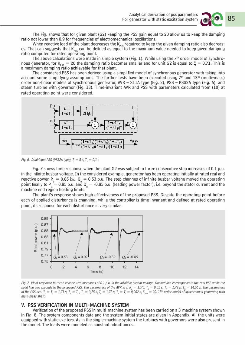
The considered PSS has been derived using a simplified model of synchronous generator with taking into account some simplifying assumptions. The further tests have been executed using 7th and 13th (multi-mass) order non-linear models of synchronous generator, AVR – ST1A type (Fig. 2), PSS – PSS2A type (Fig. 6), and steam turbine with governor (Fig. 13). Time-invariant AVR and PSS with parameters calculated from (10) at rated operating point were considered.
Fig. 6. Dual-input PSS (PSS2A type), Tr = 5 s, TF = 0,1 s
Fig. 7 shows time response when the plant G2 was subject to three consecutive step increases of 0.1 p.u. in the infinite busbar voltage. In the considered example, generator has been operating initially at rated real and reactive power, Pg = 0,85 j.w., Qg = 0,53 p.u. The step changes of infinite busbar voltage moved the operating point finally to Pg = 0.85 p.u. and Qg = -0.85 p.u. (leading power factor), i.e. beyond the stator current and the machine end region heating limits.
The plant’s response shows high effectiveness of the proposed PSS. Despite the operating point before each of applied disturbance is changing, while the controller is time-invariant and defined at rated operating point, its response for each disturbance is very similar.
Fig. 7. Plant response to three consecutive increases of 0.1 p.u. in the infinitive busbar voltage. Dashed line corresponds to the real PSS while the solid line corresponds to the proposed PSS. The parameters of the AVR are: KA = 1170, TA = 0,01 s, TC = 1,72 s, TB = 14,66 s. The parameters of the PSS are: Ta = T3 = 1,71 s, Tb = TA , Tc = 0,25 s, Td = 1,72 s, Te = Tf = 0,002 s, KPSS = 20. 13th order model of synchronous generator, with multi-mass shaft.
V. PSS VERIFICATION IN MULTI-MACHINE SYSTEMVerification of the proposed PSS in multi-machine system has been carried on a 3-machine system shown
in Fig. 8. The system components data and the system initial states are given in Appendix. All the units were equipped with static exciters. As in the single-machine system the turbines with governors were also present in the model. The loads were modeled as constant admittances.
85Analytical derivation of pss parameters
For generator with static excitation system
5
While using the 7th order model of synchronous generator, for KPSS = 20 the damping ratio becomes smaller and for unit G2 is equal to ξ = 0.71. This is a maximum damping ratio achievable for that plant.
The considered PSS has been derived using a simplified model of synchronous generator with taking into account some simplifying assumptions. The further tests have been executed using 7th and 13th (multi-mass) order non-linear models of synchronous generator, AVR – ST1A type (Fig. 2), PSS – PSS2A type (Fig. 6), and steam turbine with governor (Fig. 13). Time-invariant AVR and PSS with parameters calculated from (10) at rated operating point were considered.
Fig. 6. Dual-input PSS (PSS2A type), Tr = 5 s, TF = 0.1 s.
Fig. 7 shows time response when the plant G2 was subject to three consecutive step increases of 0.1 p.u. in the infinite busbar voltage. In the considered example, generator has been operating initially at rated real and reactive power, Pg = 0.85 p.u. and Qg = 0.53 p.u. The step changes of infinite busbar voltage moved the operating point finally to Pg = 0.85 p.u. and Qg = -0.85 p.u. (leading power factor), i.e. beyond the stator current and the machine end region heating limits.
The plant’s response shows high effectiveness of the proposed PSS. Despite the operating point before each of applied disturbance is changing, while the controller is time-invariant and defined at rated operating point, its response for each disturbance is very similar.
0.750.770.790.810.830.850.870.89
0 2 4 6 8 10 12 14Time (s)
Rea
l pow
er (p
.u.)
Fig. 7. Plant response to three consecutive increases of 0.1 p.u. in the infinitive busbar voltage. Dashed line corresponds to the real PSS while the solid line corresponds to the proposed PSS. The parameters of the AVR are: KA = 1170, TA = 0.01 s, TC = 1.72 s, TB = 14.66 s. The parameters of the PSS are: Ta = T3 = 1.71 s, Tb = TA , Tc = 0.25 s, Td = 1.72 s, Te = Tf = 0.002 s, KPSS= 20. 13th order model of synchronous generator, with multi-mass shaft.
V. PSS VERIFICATION IN MULTI-MACHINE SYSTEM
Verification of the proposed PSS in multi-machine system has been carried on a 3-machine system shown in Fig. 8. The system components data and the system initial states are given in Appendix. All the units were equipped with static exciters.
As in the single-machine system the turbines with governors were also present in the model. The loads were modeled as constant admittances.
The PSS and AVR time constants for each unit have been calculated in a single-machine model with data of a given generator and AVR, at the rated operating point, with external impedance equal to Zs = 0.001+j0.1 p.u. (related to given machine rated apparent power). The AVR time constant TB has been recalculated to keep original (as in Tab. VII) quotient of TB/TC. The calculated PSS and AVR parameters are presented in Tab. I.
1
G1
426
5 3
G3
G2
P5+jQ5
P6+jQ6 P4+jQ4
Fig. 8. Three-machine power system model
There were considered two cases: Case 1: Relatively short and low loaded transmission lines.
The generators operated at approximately rated real power and with close to zero reactive power, i.e. with relatively low stability margin.
Case 2: System with disconnected line 2-4. Lines 1-6 and 6-2 with doubled length. Reactive loads almost doubled, what caused that the lines were more loaded in comparison to the case 1. Operating point of generator G3 was close to the rated one while generator G2, with weakest connection to the other generators, was operating with almost rated real power and with small reactive power.
Fig. 9 illustrates root locus for the considered 3-machine system, in case 1. The low damped modes are presented only. The Fig. shows root locus as a functions of the PSS gain in case when the all gains takes the same value, i.e. KPSS1 = KPSS2= KPSS3. The gains are changing from 0 to 30, with step equal to 3. Roots related to the PSS gain equal to zero are marked by triangle while the one related to gain equal to 30 are marked by square.
In considered case the local modes Mi tend to the common area while frequency of modes which are measure of inter-machine oscillations Ni tend to zero. High increase of the PSSs gain lead to coherent oscillations of the units’ rotors, i.e. frequency of the modes Mi becomes equal to each other while frequencies of the modes Ni becomes equal to zero. In such case, maximal damping, defined by weakest-damped mode, achievable for this system becomes equal to about ξ = 0.4.
Minimal damping in the system is defined by mode M3(unit’s G3 local mode) which, for the PSS gain KPSSi > 3, becomes the weakest-damped mode.
The identical value of the each PSS gain causes here, relatively high and long lasting overshoots of voltages during
Qg = 0.53 Qg = 0.07 Qg = -0.39 Qg = -0.85
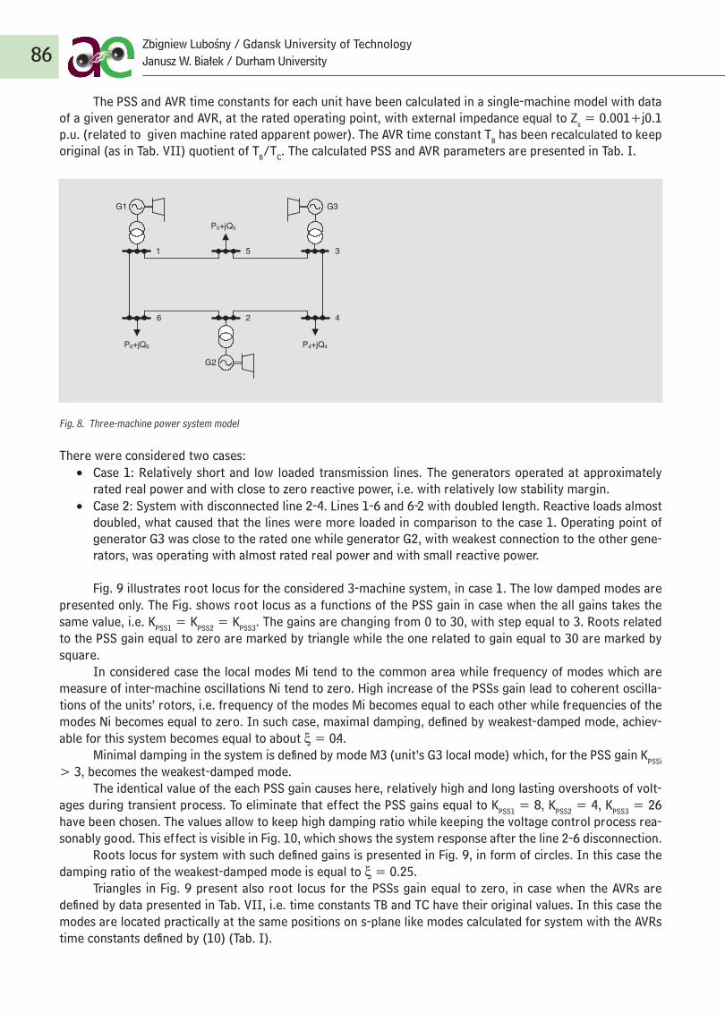
The PSS and AVR time constants for each unit have been calculated in a single-machine model with data of a given generator and AVR, at the rated operating point, with external impedance equal to Zs = 0.001+j0.1 p.u. (related to given machine rated apparent power). The AVR time constant TB has been recalculated to keep original (as in Tab. VII) quotient of TB/TC. The calculated PSS and AVR parameters are presented in Tab. I.
Fig. 8. Three-machine power system model
There were considered two cases:• Case 1: Relatively short and low loaded transmission lines. The generators operated at approximately
rated real power and with close to zero reactive power, i.e. with relatively low stability margin. • Case 2: System with disconnected line 2-4. Lines 1-6 and 6-2 with doubled length. Reactive loads almost
doubled, what caused that the lines were more loaded in comparison to the case 1. Operating point of generator G3 was close to the rated one while generator G2, with weakest connection to the other gene-rators, was operating with almost rated real power and with small reactive power.
Fig. 9 illustrates root locus for the considered 3-machine system, in case 1. The low damped modes are presented only. The Fig. shows root locus as a functions of the PSS gain in case when the all gains takes the same value, i.e. KPSS1 = KPSS2 = KPSS3. The gains are changing from 0 to 30, with step equal to 3. Roots related to the PSS gain equal to zero are marked by triangle while the one related to gain equal to 30 are marked by square.
In considered case the local modes Mi tend to the common area while frequency of modes which are measure of inter-machine oscillations Ni tend to zero. High increase of the PSSs gain lead to coherent oscilla-tions of the units’ rotors, i.e. frequency of the modes Mi becomes equal to each other while frequencies of the modes Ni becomes equal to zero. In such case, maximal damping, defined by weakest-damped mode, achiev-able for this system becomes equal to about ξ = 0.4.
Minimal damping in the system is defined by mode M3 (unit’s G3 local mode) which, for the PSS gain KPSSi > 3, becomes the weakest-damped mode.
The identical value of the each PSS gain causes here, relatively high and long lasting overshoots of volt-ages during transient process. To eliminate that effect the PSS gains equal to KPSS1 = 8, KPSS2 = 4, KPSS3 = 26 have been chosen. The values allow to keep high damping ratio while keeping the voltage control process rea-sonably good. This effect is visible in Fig. 10, which shows the system response after the line 2-6 disconnection.
Roots locus for system with such defined gains is presented in Fig. 9, in form of circles. In this case the damping ratio of the weakest-damped mode is equal to ξ = 0.25.
Triangles in Fig. 9 present also root locus for the PSSs gain equal to zero, in case when the AVRs are defined by data presented in Tab. VII, i.e. time constants TB and TC have their original values. In this case the modes are located practically at the same positions on s-plane like modes calculated for system with the AVRs time constants defined by (10) (Tab. I).
86Zbigniew Lubośny / Gdansk University of TechnologyJanusz W. Białek / Durham University
13
1
G1
426
5 3
G3
G2
P5+jQ5
P6+jQ6 P4+jQ4
Rys. 8. Struktura systemu trzymaszynowego
RozwaŜano dwa warianty pracy systemu:
• Wariant 1: Względnie krótkie i dość słabo obciąŜone linie elektroenergetyczne. Punkty pracy
generatorów synchronicznych bliskie granicy stabilności lokalnej, ze znamionową generacją mocy
czynnej
• Wariant 2: System z wyłączoną linią 2–4. Linie 1–6 i 6–2 o zdwojonej, w stosunku do wariantu 1,
długości. ObciąŜenia mocą bierną w węzłach odbiorczych równieŜ zdwojone. Punkt pracy generatora
G3 zbliŜony do znamionowego. Generator G2, najsłabiej związany z resztą systemu
elektroenergetycznego, obciąŜony praktycznie znamionową mocą czynną i małą mocą bierną.
Rys. 9 przedstawia rozmieszczenie biegunów układu trzymaszynowego (zlinearyzowanego) dla wariantu 1,
przy czym prezentowane są tu tylko wartości własne najsłabiej tłumionych modów. Pokazano tu zaleŜność
połoŜenia biegunów od współczynnika wzmocnienia stabilizatorów systemowych, gdy wartości tych
współczynników dla wszystkich trzech stabilizatorów są sobie równe, tj. KPSS1 = KPSS2 = KPSS3. Wartości
tych współczynników zmieniają się w przedziale od 0 do 30, z krokiem równym 3. Wartości własne dla
współczynnika wzmocnienia stabilizatorów systemowych równego 0 (zero) oznaczone są trójkątami, a dla
równego 30-kwadratami.
W prezentowanym przypadku, w miarę wzrostu wartości współczynnika wzmocnienia stabilizatora
systemowego, mody kołysań lokalnych Mi zmierzają do wspólnego obszaru, natomiast częstotliwości
modów będących miarą kołysań międzyobszarowych (międzygeneratorowych) Ni zmierzają do zera.
Wzrost współczynników wzmocnienia stabilizatorów systemowych powoduje, Ŝe kołysania wirników
generatorów stają się koherentne, tzn. częstotliwości modów kołysań lokalnych Mi stają się sobie równe, a
częstotliwości kołysań między obszarowych (międzygeneratorowych) Ni dąŜą do zera. W tym przypadku
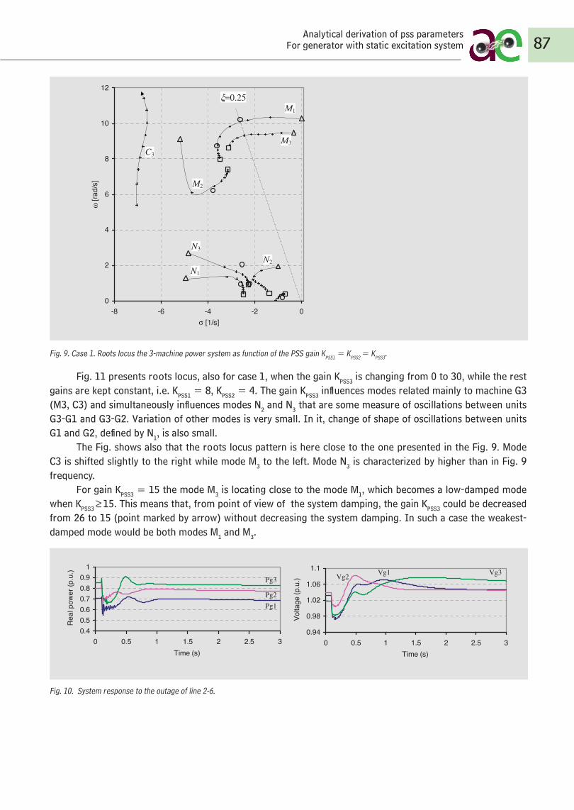
Fig. 9. Case 1. Roots locus the 3-machine power system as function of the PSS gain KPSS1 = KPSS2 = KPSS3.
Fig. 11 presents roots locus, also for case 1, when the gain KPSS3 is changing from 0 to 30, while the rest gains are kept constant, i.e. KPSS1 = 8, KPSS2 = 4. The gain KPSS3 influences modes related mainly to machine G3 (M3, C3) and simultaneously influences modes N2 and N3 that are some measure of oscillations between units G3-G1 and G3-G2. Variation of other modes is very small. In it, change of shape of oscillations between units G1 and G2, defined by N1, is also small.
The Fig. shows also that the roots locus pattern is here close to the one presented in the Fig. 9. Mode C3 is shifted slightly to the right while mode M3 to the left. Mode N3 is characterized by higher than in Fig. 9 frequency.
For gain KPSS3 = 15 the mode M3 is locating close to the mode M1, which becomes a low-damped mode when KPSS3 ≥ 15. This means that, from point of view of the system damping, the gain KPSS3 could be decreased from 26 to 15 (point marked by arrow) without decreasing the system damping. In such a case the weakest-damped mode would be both modes M1 and M3.
Fig. 10. System response to the outage of line 2-6.
87Analytical derivation of pss parameters
For generator with static excitation system
14
maksymalne tłumienie kołysań elektromechanicznych, definiowane przez współczynnik tłumienia modu
najsłabiej tłumionego, jest równe ξ = 0,4.
Minimalne tłumienie w systemie określa mod M3 (mod kołysań lokalnych generatora G3), który dla KPSSi >
3 staje się modem najsłabiej tłumionym.
Przyjęcie jednakowych wartości współczynnika wzmocnienia wszystkich stabilizatorów systemowych
powoduje tu występowanie względnie duŜych i długo trwających przeregulowań napięcia generatorów w
odpowiedzi na zaburzenie stanu pracy układu. W celu wyeliminowania tego efektu przyjęto wartości
współczynników wzmocnienia równe KPSS1 = 8, KPSS2 = 4, KPSS3 = 26. Wartości te pozwalają utrzymać
dobre tłumienie kołysań elektromechanicznych, zapewniając równocześnie dobre odpowiedzi napięciowe
generatorów. Uzyskany w tym przypadku efekt przedstawiono na rys. 10, pokazującym odpowiedź układu
na wyłączenie linii 2–6.
Rozmieszczenie biegunów na rys. 9 przedstawiają kółka, współczynnik tłumienia najsłabiej tłumionego
modu elektromechanicznego jest równy ξ = 0,25.
Trójkąty na rys. 9 przedstawiają równieŜ połoŜenie biegunów układu dla zerowych wartości
współczynnika wzmocnienia i równocześnie dla parametrów regulatorów napięcia równych wartościom
tzw. oryginalnym, przedstawionym w tab. VII, tj. z rzeczywistymi (z obiektów rzeczywistych) wartościami
stałych czasowych TB i TC. W tym przypadku lokalizacja wartości własnych jest praktycznie identyczna jak
lokalizacja wartości własnych dla obliczenia regulatorów napięcia z wartościami parametrów obliczonymi
na podstawie zaleŜności (10) (tab. I).
0
2
4
6
8
10
12
-8 -6 -4 -2 0σ [1/s]
ω [r
ad/s
]
N1
N2
N3
M2
M1
M3
C3
ξ=0.25
6
transient process. To eliminate that effect the PSS gains equal to KPSS1 = 8, KPSS2 = 4, KPSS3 = 26 have been chosen. The values allow to keep high damping ratio while keeping the voltage control process reasonably good. This effect is visible in Fig. 10, which shows the system response after the line 2-6 disconnection.
Roots locus for system with such defined gains is presented in Fig. 9, in form of circles. In this case the damping ratio of the weakest-damped mode is equal to ξ = 0.25.
Triangles in Fig. 9 present also root locus for the PSSs gain equal to zero, in case when the AVRs are defined by data presented in Tab. VII, i.e. time constants TB and TC have their original values. In this case the modes are located practically at the same positions on s-plane like modes calculated for system with the AVRs time constants defined by (10) (Tab. I).
0
2
4
6
8
10
12
-8 -6 -4 -2 0σ [1/s]
ω [r
ad/s
]
Fig. 9. Case 1. Roots locus the 3-machine power system as function of the PSS gain KPSS1 = KPSS2 = KPSS3.
Fig. 11 presents roots locus, also for case 1, when the gain KPSS3 is changing from 0 to 30, while the rest gains are kept constant, i.e. KPSS1 = 8, KPSS2 = 4. The gain KPSS3 influences modes related mainly to machine G3 (M3, C3) and simultaneously influences modes N2 and N3 that are some measure of oscillations between units G3-G1 and G3-G2. Variation of other modes is very small. In it, change of shape of oscillations between units G1 and G2, defined by N1, is also small.
The Fig. shows also that the roots locus pattern is here close to the one presented in the Fig. 9. Mode C3 is shifted slightly to the right while mode M3 to the left. Mode N3 is characterized by higher than in Fig. 9 frequency.
For gain KPSS3 = 15 the mode M3 is locating close to the mode M1, which becomes a low-damped mode when KPSS3 ≥15. This means that, from point of view of the system damping, the gain KPSS3 could be decreased from 26 to 15 (point marked by arrow) without decreasing the system
damping. In such a case the weakest-damped mode would be both modes M1 and M3.
0.40.50.60.70.80.9
1
0 0.5 1 1.5 2 2.5 3Time (s)
Real
pow
er (p
.u.)
0.94
0.98
1.02
1.06
1.1
0 0.5 1 1.5 2 2.5 3Time (s)
Volta
ge (p
.u.)
Fig. 10. System response to the outage of line 2-6.
0
2
4
6
8
10
12
-8 -6 -4 -2 0σ [1/s]
ω [r
ad/s
]
Fig. 11. Case 1. Roots locus in the 3-machine power system as function of the PSS gain KPSS3.
Finally, Fig. 12 illustrates roots locus for the 3-machine system, in case 2. As previously, the all PSSs gain is equal to each other and changes from 0 to 30. Like in the previous case the circles show root locus for system with various gains (KPSS1= 8, KPSS2= 4, KPSS3= 26).
Maximum damping, achievable for this system, for KPSSi >> 30, is also equal to about ξ = 0.4. For the PSSs with various gains the damping ratio of the weakest-damped mode is equal to ξ = 0.24, which is practically the same value like in the case 1.
The minimal damping in the system is defined by mode M1, until the PSS gain KPSSi will reach 21. Next, the damping ratio
Pg1Pg2
Pg3
Vg2 Vg1 Vg3
N1
N2
N3
M2
M1
M3
C3
ξ=0.25
M3
M1
M2
C3
N2
N3
N1
KPSS3 =15
6
transient process. To eliminate that effect the PSS gains equal to KPSS1 = 8, KPSS2 = 4, KPSS3 = 26 have been chosen. The values allow to keep high damping ratio while keeping the voltage control process reasonably good. This effect is visible in Fig. 10, which shows the system response after the line 2-6 disconnection.
Roots locus for system with such defined gains is presented in Fig. 9, in form of circles. In this case the damping ratio of the weakest-damped mode is equal to ξ = 0.25.
Triangles in Fig. 9 present also root locus for the PSSs gain equal to zero, in case when the AVRs are defined by data presented in Tab. VII, i.e. time constants TB and TC have their original values. In this case the modes are located practically at the same positions on s-plane like modes calculated for system with the AVRs time constants defined by (10) (Tab. I).
0
2
4
6
8
10
12
-8 -6 -4 -2 0σ [1/s]
ω [r
ad/s
]
Fig. 9. Case 1. Roots locus the 3-machine power system as function of the PSS gain KPSS1 = KPSS2 = KPSS3.
Fig. 11 presents roots locus, also for case 1, when the gain KPSS3 is changing from 0 to 30, while the rest gains are kept constant, i.e. KPSS1 = 8, KPSS2 = 4. The gain KPSS3 influences modes related mainly to machine G3 (M3, C3) and simultaneously influences modes N2 and N3 that are some measure of oscillations between units G3-G1 and G3-G2. Variation of other modes is very small. In it, change of shape of oscillations between units G1 and G2, defined by N1, is also small.
The Fig. shows also that the roots locus pattern is here close to the one presented in the Fig. 9. Mode C3 is shifted slightly to the right while mode M3 to the left. Mode N3 is characterized by higher than in Fig. 9 frequency.
For gain KPSS3 = 15 the mode M3 is locating close to the mode M1, which becomes a low-damped mode when KPSS3 ≥15. This means that, from point of view of the system damping, the gain KPSS3 could be decreased from 26 to 15 (point marked by arrow) without decreasing the system
damping. In such a case the weakest-damped mode would be both modes M1 and M3.
0.40.50.60.70.80.9
1
0 0.5 1 1.5 2 2.5 3Time (s)
Real
pow
er (p
.u.)
0.94
0.98
1.02
1.06
1.1
0 0.5 1 1.5 2 2.5 3Time (s)
Volta
ge (p
.u.)
Fig. 10. System response to the outage of line 2-6.
0
2
4
6
8
10
12
-8 -6 -4 -2 0σ [1/s]
ω [r
ad/s
]
Fig. 11. Case 1. Roots locus in the 3-machine power system as function of the PSS gain KPSS3.
Finally, Fig. 12 illustrates roots locus for the 3-machine system, in case 2. As previously, the all PSSs gain is equal to each other and changes from 0 to 30. Like in the previous case the circles show root locus for system with various gains (KPSS1= 8, KPSS2= 4, KPSS3= 26).
Maximum damping, achievable for this system, for KPSSi >> 30, is also equal to about ξ = 0.4. For the PSSs with various gains the damping ratio of the weakest-damped mode is equal to ξ = 0.24, which is practically the same value like in the case 1.
The minimal damping in the system is defined by mode M1, until the PSS gain KPSSi will reach 21. Next, the damping ratio
Pg1Pg2
Pg3
Vg2 Vg1 Vg3
N1
N2
N3
M2
M1
M3
C3
ξ=0.25
M3
M1
M2
C3
N2
N3
N1
KPSS3 =15
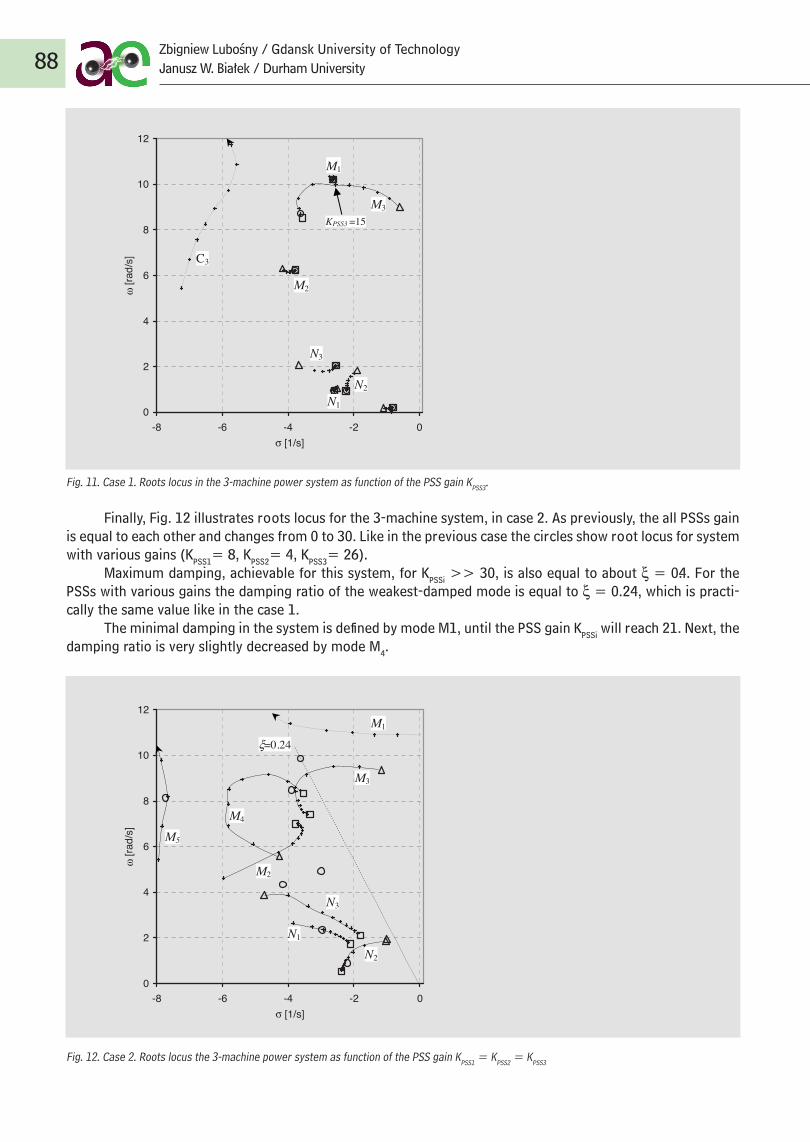
Fig. 11. Case 1. Roots locus in the 3-machine power system as function of the PSS gain KPSS3.
Finally, Fig. 12 illustrates roots locus for the 3-machine system, in case 2. As previously, the all PSSs gain is equal to each other and changes from 0 to 30. Like in the previous case the circles show root locus for system with various gains (KPSS1= 8, KPSS2= 4, KPSS3= 26).
Maximum damping, achievable for this system, for KPSSi >> 30, is also equal to about ξ = 0.4. For the PSSs with various gains the damping ratio of the weakest-damped mode is equal to ξ = 0.24, which is practi-cally the same value like in the case 1.
The minimal damping in the system is defined by mode M1, until the PSS gain KPSSi will reach 21. Next, the damping ratio is very slightly decreased by mode M4.
Fig. 12. Case 2. Roots locus the 3-machine power system as function of the PSS gain KPSS1 = KPSS2 = KPSS3
88Zbigniew Lubośny / Gdansk University of TechnologyJanusz W. Białek / Durham University
16
0
2
4
6
8
10
12
-8 -6 -4 -2 0σ [1/s]
ω [r
ad/s
]
Rys. 11. Wariant 1. Lokalizacja biegunów układu trzymaszynowego w funkcji współczynnika
wzmocnienia stabilizatora systemowego KPSS3
Na zakończenie, rys. 12 przedstawia połoŜenie modów systemu dla wariantu 2. Jak poprzednio,
współczynniki wzmocnienia stabilizatorów systemowych, równe sobie, zmieniają się od 0 do 30. RównieŜ
jak poprzednio, kółka pokazują połoŜenia biegunów układu dla systemu z róŜnymi współczynnikami
wzmocnienia stabilizatorów systemowych, równych odpowiednio KPSS1 = 8, KPSS2 = 4, KPSS3 = 26.
Maksymalne tłumienie kołysań w tym systemie, osiągane dla KPSSi >> 30, jest równieŜ równe około ξ =
0,4. W przypadku systemu z róŜnymi współczynnikami wzmocnienia współczynnik tłumienia najsłabiej
tłumionego modu jest równy ξ = 0,24, co jest wartością porównywalną z uzyskaną poprzednio (w
wariancie 1).
Minimalne tłumienie w układzie określa mod M1 do chwili, gdy współczynnik wzmocnienia KPSSi osiąga
wartość 21. Dalej współczynnik tłumienia jest słabo ograniczany przez mod M4.
M3
M1
M2
C3
N2
N3
N1
KPSS3 =15
17
0
2
4
6
8
10
12
-8 -6 -4 -2 0σ [1/s]
ω [r
ad/s
]
Rys. 12. Wariant 2. Lokalizacja biegunów układu trzymaszynowego w funkcji współczynników
wzmocnienia stabilizatorów systemowych dla przypadku KPSS1 = KPSS2 = KPSS3
VI. WNIOSKI
W artykule przedstawiono sposób analitycznego określania parametrów stabilizatora systemowego
quasi-idealnego, tj. takiego, który wytwarza tylko moment tłumiący w szerokim przedziale zmian
częstotliwości kołysań elektromechanicznych. Metoda oparta jest na modelu generatora synchronicznego 3.
rzędu i zastosowana dla generatora ze statycznym układem wzbudzenia i regulacji napięcia oraz
stabilizatora systemowego z prędkością kątową wirnika jako sygnałem wejściowym. Metoda jest czuła na
strukturę regulatora napięcia, zatem zaleŜności pozwalające określać nastawy stabilizatora systemowego
zaleŜą od przyjętej struktury regulatora. W artykule przedstawiono zaleŜności dla jednej struktury
regulatora napięcia i jej dwóch podstruktur.
Wartości parametrów stabilizatora zaleŜą od danych obiektu (generatora), danych regulatora napięcia,
punktu pracy generatora oraz impedancji zewnętrznej. PoniewaŜ dwie ostatnie wielkości są zmienne w
trakcie pracy systemu, optymalny stabilizator systemowy powinien charakteryzować się zmiennymi
wartościami parametrów. W praktyce stosuje się jednak stabilizatory (a takŜe regulator napięcia)
stacjonarne. Przeprowadzone testy wykazały, Ŝe równieŜ proponowany stabilizator systemowy jest
efektywny w wariancie stacjonarnym.
PoniewaŜ parametry stabilizatora systemowego związane są z parametrami regulatora napięcia, wartości
niektórych parametrów regulatora napięcia powinny być określane równocześnie z wartościami
N2
N3
N1
M1
M2
M5
M3
M4
ξ=0.24
VI. CONCLUSIONSThe paper presents way of deriving equations that allow to calculate parameters of PSS that produces
a damping torque only in a wide frequency range. The derivation is based on the 3rd order single-machine infinite-busbar model and is applied here for generator with static exciter and speed-based PSS. Because the method is the AVR structure sensitive, as result, three sets of equations allowing to calculate PSS parameters for three various structures of AVR are presented.
The PSS parameters defined by proposed equations depend on plant data, AVR parameters, system op-erating point and external impedance. Because of the latter two, the PSS parameters should vary during plant operation but tests have proved that the proposed PSS in form of a time-invariant controller performs almost equally well.
The PSS parameters are related to some of the AVR parameters and therefore should be set simultane-ously.
Advantage of the proposed methodology is simplicity of the PSS design. PSS time constants can be cal-culated directly, using a single-machine steady-state model, without any iterative optimization process. Simula-tions have shown that the values derived in a single-machine system (by applying the proposed equations) are valid also in a multi-machine system.
The proposed method has been verified for large units operating in transmission system and for smaller units operating in distribution systems (results not presented here) giving in the all cases good results. The method seems to be especially suited for units operating in the distribution systems because the distribution systems operates as radial and the transmission system, from point of view of such units, can be treated as in-finite busbar. Then solution achieved for the single-machine system directly match to generating unit operating in the distribution system.
Low amount and accessibility of data that is necessary to calculate the PSS (and AVR) parameters allow us to implement the derived equations in any digital controller of synchronous generator. In such a case the PSS parameters and some AVR parameters can be calculated just by the synchronous generator controller.
The equations proposed in the paper allow us to define PSS that effectiveness is similar to effectiveness of the well tuned PSS, which parameters are defined by using GEP or P-Vr methodology. This is because the all mentioned methods are based on damping torque concept and, especially because they utilize the same struc-ture of PSS, which in fact defines limits of such PSS efficiency.
VIII. APPENDIX
A. Linear model of single-machine infinite busbar system
X’d = Xl+Xad− Xad×Xad/Xf
RT = Rl+Rt+Rs, XTq = Xq+Xt+Xs, XTd = X’d+Xt+Xs
D = RT×RT+XTd×XTq
m1 = Vs(XTq×sinδ−RT
×cosδ)/D, n1 = Vs (RT×sinδ+XTd
×cosδ)/D
m2 = XTq×Xad/(D×Xf), n2 = RT
×Xad/(D×Xf)
K1 = Eq×n1+Iq
×(Xq-X’d)m1
K2 = Xad[RT×Eq/D+(1+XTq
×(Xq− X’d)/D)Iq]/Xf
K3 = Xf/[Xadu×(1+(Xd−X’d)×XTq/D)], K4 = Xadu
×Xad×m1/Xf
K5 = (-Rl×m1+Xq
×n1) sinδ+(−Rl×n1-X’d×m1)cosδ
K6 = (−Rl×m2+Xq
×n2)sinδ+[−Rl×n2-X’d×m2+(X’d−Xl)/(Xf-Xad)]cosδ
T3 = Xf/[ω0×Rf(1+XTq(Xd−X’d)/D)]
89Analytical derivation of pss parameters
For generator with static excitation system
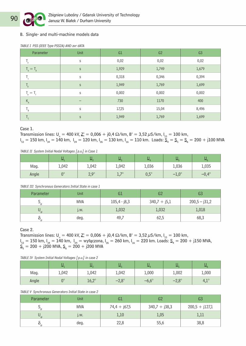
B. Single- and multi-machine models data
TABLE I PSS (IEEE Type PSS2A) AND avr dATA
Parameter Unit G1 G2 G3
Ta s 0,02 0,02 0,02
Tb = TA s 1,929 1,749 1,679
Tc s 0,318 0,346 0,394
Td s 1,949 1,769 1,699
Te = Tf s 0,002 0,002 0,002
KA – 730 1170 400
TB s 17,25 15,04 8, 496
TC s 1,949 1,769 1,699
Case 1.Transmission lines: Un = 400 kV, Z’ = 0,006 + j0, 4 Ω/km, B’ = 3,52 µS/km, l15 = 100 km, l53 = 150 km, l34 = 140 km, l24 = 120 km, l26 = 130 km, l16 = 110 km. Loads: S4 = S5 = S6 = 200 + j100 MVA
TABLE II System Initial Nodal Voltages [p.u.] in Case 1
U1 U2 U3 U4 U5 U6
Mag. 1,042 1,042 1,042 1,036 1,036 1,035
Angle 0° 2,9° 1,7° 0,5° –1,0° –0, 4°
TABLE III Synchronous Generators Initial State in case 1
Parameter Unit G1 G2 G3
Sgi MVA 105, 4 - j8,3 340,7 + j5,1 200,5 – j31,2
Ugi j.w. 1,032 1,032 1,018
δgideg. 49,7 62,5 68,3
Case 2. Transmission lines: Un = 400 kV, Z’ = 0,006 + j0, 4 Ω/km, B’ = 3,52 µS/km, l15 = 100 km, l53 = 150 km, l34 = 140 km, l24 = wyłączona, l26 = 260 km, l16 = 220 km. Loads: S4 = 200 + j150 MVA, S5 = 200 + j200 MVA, S6 = 200 + j200 MVA
TABLE IV System Initial Nodal Voltages [p.u.] in case 2
U1 U2 U3 U4 U5 U6
Mag. 1,042 1,042 1,042 1,000 1,002 1,000
Angle 0° 16,2° –2,8° –6,6° –2,8° 4,1°
TABLE V Synchronous Generators Initial State in case 2
Parameter Unit G1 G2 G3
Sgi MVA 74, 4 + j67,5 340,7 + j38,3 200,5 + j127,1
Ugi j.w. 1,10 1,05 1,11
δgideg. 22,8 55,6 38,8
90Zbigniew Lubośny / Gdansk University of TechnologyJanusz W. Białek / Durham University
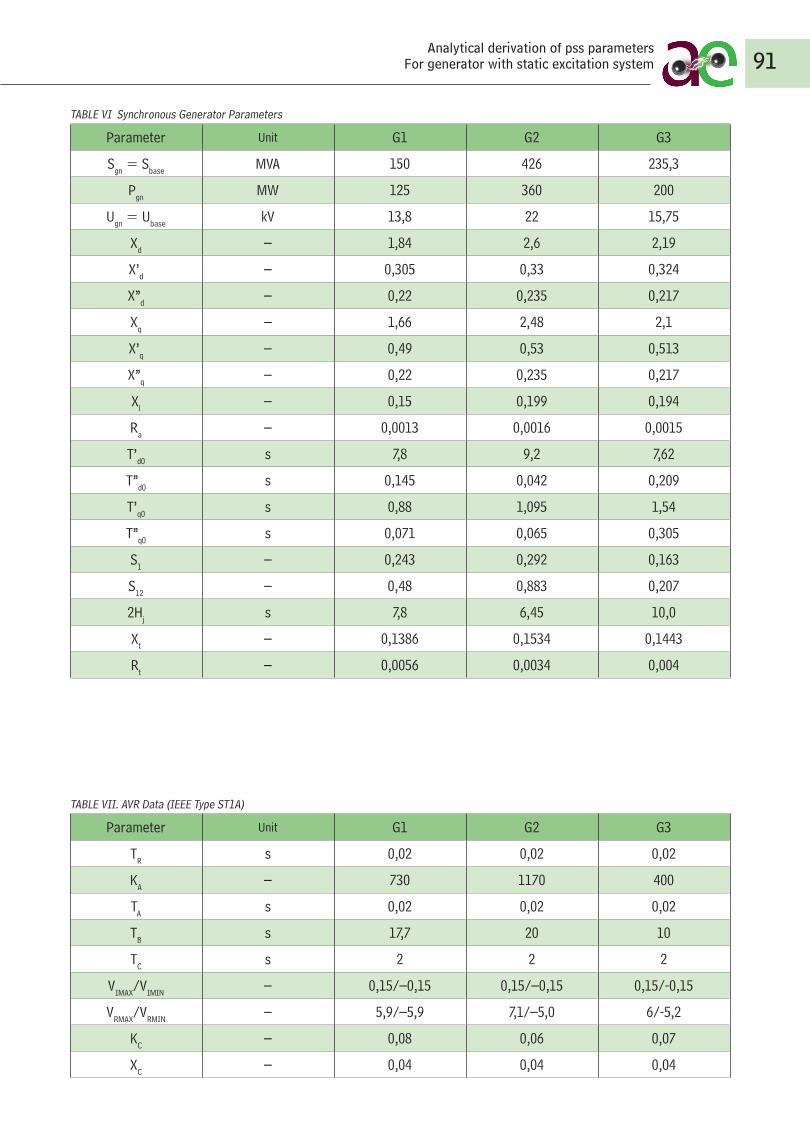
TABLE VI Synchronous Generator Parameters
Parameter Unit G1 G2 G3
Sgn = Sbase MVA 150 426 235,3
Pgn MW 125 360 200
Ugn = Ubase kV 13,8 22 15,75
Xd – 1,84 2,6 2,19
X’d – 0,305 0,33 0,324
X”d – 0,22 0,235 0,217
Xq – 1,66 2, 48 2,1
X’q – 0, 49 0,53 0,513
X”q – 0,22 0,235 0,217
Xl – 0,15 0,199 0,194
R a – 0,0013 0,0016 0,0015
T’d0 s 7,8 9,2 7,62
T”d0 s 0,145 0,042 0,209
T’q0 s 0,88 1,095 1,54
T”q0 s 0,071 0,065 0,305
S1 – 0,243 0,292 0,163
S12 – 0, 48 0,883 0,207
2Hj s 7,8 6, 45 10,0
Xt – 0,1386 0,1534 0,1443
Rt – 0,0056 0,0034 0,004
TABLE VII. AVR Data (IEEE Type ST1A)
Parameter Unit G1 G2 G3
TR s 0,02 0,02 0,02
KA – 730 1170 400
TA s 0,02 0,02 0,02
TB s 17,7 20 10
TC s 2 2 2
VIMAX/VIMIN – 0,15/–0,15 0,15/–0,15 0,15/-0,15
VRMAX/VRMIN – 5,9/–5,9 7,1/–5,0 6/-5,2
KC – 0,08 0,06 0,07
XC – 0,04 0,04 0,04
91Analytical derivation of pss parameters
For generator with static excitation system
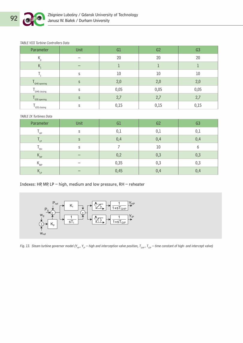
TABLE VIII Turbine Controllers Data
Parameter Unit G1 G2 G3
Kp – 20 20 20
KI – 1 1 1
TI s 10 10 10
TGHP, opening s 2,0 2,0 2,0
TGHP, closing s 0,05 0,05 0,05
TGIP, opening s 2,7 2,7 2,7
TGIP, closing s 0,15 0,15 0,15
TABLE IX Turbines Data
Parameter Unit G1 G2 G3
THP s 0,1 0,1 0,1
TLP s 0, 4 0, 4 0, 4
TRH s 7 10 6
KHP – 0,2 0,3 0,3
KMP – 0,35 0,3 0,3
KLP – 0, 45 0, 4 0, 4
Indexes: HP, MP, LP – high, medium and low pressure, RH – reheater
Fig. 13. Steam turbine governor model (YHP , YIP – high and interception valve position, TGHP , TGIP – time constant of high- and intercept valve)
92Zbigniew Lubośny / Gdansk University of TechnologyJanusz W. Białek / Durham University
22
miary
THP s 0,1 0,1 0,1
TLP s 0,4 0,4 0,4
TRH s 7 10 6
KHP – 0,2 0,3 0,3
KMP – 0,35 0,3 0,3
KLP – 0,45 0,4 0,4
Indeksy: HP, MP, LP – wysoko-, średnio- i niskopręŜny, RH – przegrzewacz międzystopniowy.
KI
1sTI
11
11 1
1+sTGHP
YHP
YIP
Pref
wref
Pg
Kp
wg 11+sTGIP
Rys. 13. Model regulatora turbiny (YHP, YIP – połoŜenie zaworów wysokopręŜnych i intercepcyjnych
turbiny, TGHP, TGIP – stałe czasowe zaworów wysokopręŜnych i intercepcyjnych)
Bibliografia
1. IEEE Std 421.5-1992: IEE Recommended Practice for Excitation System Models for Power System
Stability Studies, IEEE, New York 1992, ISBN 1–55937–218–4.
2. Mello de F.P., Concordia C., Concepts of Synchronous Machine Stability as Affected by Excitation
Control, IEEE Trans. Power Appar. Syst., vol. 88, 1969, s. 316–329.
3. Larsen E.V., Swann D.A., Applying Power System Stabilizer, IEEE Trans. Power Appar. Syst., vol. 100,
1981, s. 3017–3046.
4. Mello de F.P., Czuba J.S., Rushe P.A., Willis J.R., Developments in Application of Stabilising Measures
Through Excitation Control, Paper Ref. 38-05, CIGRE Session 1986.
5. Gibbard M.J., Co-ordinated design of multimachine power system stabilizers based on damping torque
concept, Proc. Inst. Elect. Eng. C, vol. 135, no. 4, July 1988, s. 276–284.
6. Gibbard M.J., Robust Design of Fixed-parameter Power System Stabilisers over a Wide Range of
Operating Conditions, IEEE Trans. Power Syst., vol. 6, no. 2, May 1991, s. 794–800.
7. Gibbard M. J., Vowles D. J., Reconciliation of Methods of Compensation for PSSs in Multimachine
System, IEEE Trans. Power Syst., vol. 19, no. 1, February 2004, s. 463–472.
8. Kundur P., Power system stability and control, New York: McGraw–Hill, 1994, s. 761.
Σ Σ
Σ
LITERATURE
1. IEEE Std 421.5-1992: IEE Recommended Practice for Excitation System Models for Power System Stability Studies, IEEE, New York 1992, ISBN 1–55937–218–4.
2. Mello de F.P., Concordia C., Concepts of Synchronous Machine Stability as Affected by Excitation Control, IEEE Trans. Power Appar. Syst., vol. 88, 1969, s. 316–329.
3. Larsen E.V., Swann D.A., Applying Power System Stabilizer, IEEE Trans. Power Appar. Syst., vol. 100, 1981, s. 3017–3046.4. Mello de F.P., Czuba J.S., Rushe P.A., Willis J.R., Developments in Application of Stabilising Measures Through Exci-
tation Control, Paper Ref. 38-05, CIGRE Session 1986.5. Gibbard M.J., Co-ordinated design of multimachine power system stabilizers based on damping torque concept,
Proc. Inst. Elect. Eng. C, vol. 135, no. 4, July 1988, s. 276–284.6. Gibbard M.J., Robust Design of Fixed-parameter Power System Stabilisers over a Wide Range of Operating Condi-
tions, IEEE Trans. Power Syst., vol. 6, no. 2, May 1991, s. 794–800.7. Gibbard M.J., Vowles D.J., Reconciliation of Methods of Compensation for PSSs in Multimachine System, IEEE Trans.
Power Syst., vol. 19, no. 1, February 2004, s. 463–472.8. Kundur P., Power system stability and control, New York: McGraw–Hill, 1994, s. 761.9. Machowski J., Bialek J., Bumby J.R., Power System Dynamics and Stability, New York: John Wiley and Sons, 1997, s. 291.10. CIGRE Task Force 38.02.16, Impact of Interactions among Power Systems, Paris, August 2000.11. CIGRE Task Force 38.01.07, Analysis and Control of Power System Oscillations, Paris, December 1996.12. Lee D.C., Kundur P., Advanced Excitation Controls for Power System Stability Enhancement, Paper Ref., no 38–01,
CIGRE Session 1986.13. Murdoch Dr.A., Venkataraman S., Lawson R.A., Pearson W.R., Integral of Accelerating Power Type PSS. Part 1 –
Theory, Design, and Tuning Methodology. Part 2 – Field Testing and Performance Verification, IEEE Trans. on Energy Conv., vol. 14, no. 4, December 1999, s. 1658–1672.
93Analytical derivation of pss parameters
For generator with static excitation system